Resolving Word Ambiguities• Description: After determining word boundaries, the speech

recognition process matches an array of possible word sequences from spoken audio

• Issues to consider – determine the intended word sequence?– resolve grammatical and pronunciation errors

• Applications: spell-checking, allophonic variations of pronunciation, automatic speech recognition

• Implementation: Establish word sequence probabilities– Use existing corpora– Train program with run-time data

Entropy

Questions answered if we can compute entropy?

• How much information there is in a particular grammar, words, parts of speech, phonemes, etc?

• How predictive is a language in computing the next word based on previous words?

• How difficult is a speech recognition task?

• Entropy is measured in bits• What is the least number of bits

required to encode a piece of information

Measures the quantity of information in a signal stream

- pi lg pi

i=1

r

åH(X) =

X is a random variable that can assume r values

Entropy of spoken languages could focus implementation possibilities

Entropy Example• Eight Horses are in an upcoming race

– We want to take bets on the winner

– Naïve approach is to use 3 bits

– Better approach is to use less bits for the horses bet on more frequently

• Entropy – What is the minimum number of bits needed?

= -∑i=1,8p(i)log p(i)

= - ½ log ½ - ¼ log ¼ - 1/8 log 1/8 – 1/16 log 1/16 – 4 * 1/64 log 1/64

= 1/2 + 2/4 +3/8 + 4/16 + 4 * 6/64 = (32 + 32 + 24 + 16 + 24)/64 = 2

• The table to the right shows the optimal coding scheme• Question: What if the odd were all equal (1/8)

Horse odds Code

1 ½ 0

2 ¼ 10

3 1/8 110

4 1/16 1110

5 1/64 111100

6 1/64 111101

7 1/64 111110

8 1/64 111111

Entropy of words and languages• What is the entropy of a sequence of words?

H(w1,w2,…,wn) = -∑ p(win) log p (wi

n)

– win ε L

– P(win) = probability that wi

n is in a sequence of n words

• What is the entropy of a word appearing in an n word sequence?

H(w1n) = - 1/n ∑ p(wi

n) log p (win)

• What is the entropy of a language?

H(L) = lim n=∞ (- 1/n * ∑ p(win) log p (wi

n))

Cross Entropy• We want to know the entropy of a language L, but don’t

know its distribution• We model L by an approximation to its probability

distribution• We take sequences of words, phonemes, etc from the real

language but use the following formula

H(p,m) = limn->∞ - 1/n log m(w1,w2,…,wn)

• Cross entropy will always be an upper bound for the actual language

• Example– Trigram model of 583 million words of English– Corpus of 1,014,312 tokens– Character entropy computed based on a tri-gram grammar– Result 1.75 bits per character

Probability Chain Rule• Conditional Probability P(A1,A2) = P(A1) · P(A2|A1)• The Chain Rule generalizes to multiple events

– P(A1, …,An) = P(A1) P(A2|A1) P(A3|A1,A2)…P(An|A1…An-1) • Examples:

– P(the dog) = P(the) P(dog | the)– P(the dog bites) = P(the) P(dog | the) P(bites| the dog)

• Conditional probability applies more than individual relative word frequencies because they consider the context – Dog may be relatively rare word in a corpus– But if we see barking, P(dog|barking) is much more likely

)11|

1( wk

n

kwkP

1n

• In general, the probability of a complete string of words w1…wn is:

P(w ) = P(w1)P(w2|w1)P(w3|w1..w2)…P(wn|w1…wn-1) =

Detecting likely word sequences using probabilities

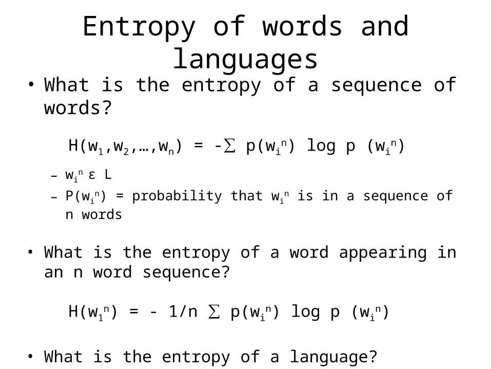
Counts• What’s the probability of “canine”?• What’s the probability of “canine tooth” or tooth | canine?• What’s the probability of “canine companion”?• P(tooth|canine) = P(canine & tooth)/P(canine)

• Sometimes we can use counts to deduce probabilities.• Example: According to google:

– P(canine): occurs 1,750,000 times– P(canine tooth): 6280 times – P(tooth | canine): 6280/1750000 = .0035– P(companion | canine): .01 – So companion is the more likely next word after canine

Detecting likely word sequences using counts/table look up

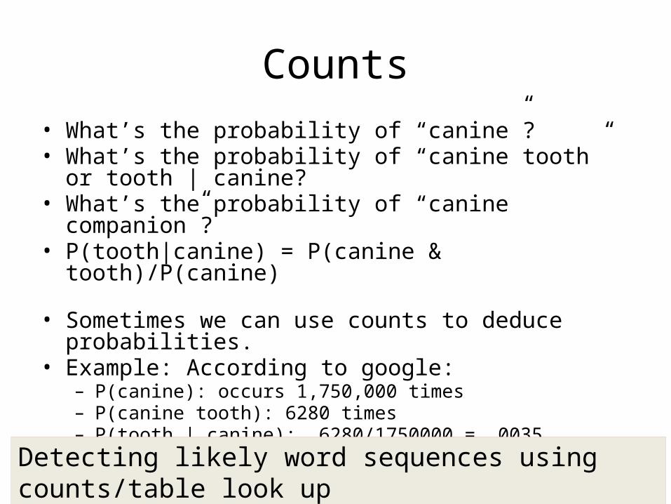
Single Word Probabilities

Word P(O|w) P(w) P(O|w)P(w)

new .36 .001 .00036

neat .52 .00013 .000068

need .11 .00056 .000062

knee 1.00 .000024 .000024

P([ni]|new)P(new)

P([ni]|neat)P(neat)

P([ni]|need)P(need)

P([ni]|knee)P(knee)

• Limitation: ignores context• We might need to factor in the surrounding words

- Use P(need|I) instead of just P(need)- Note: P(new|I) < P(need|I)

Single word probability

Compute likelihood P([ni]|w), then multiply

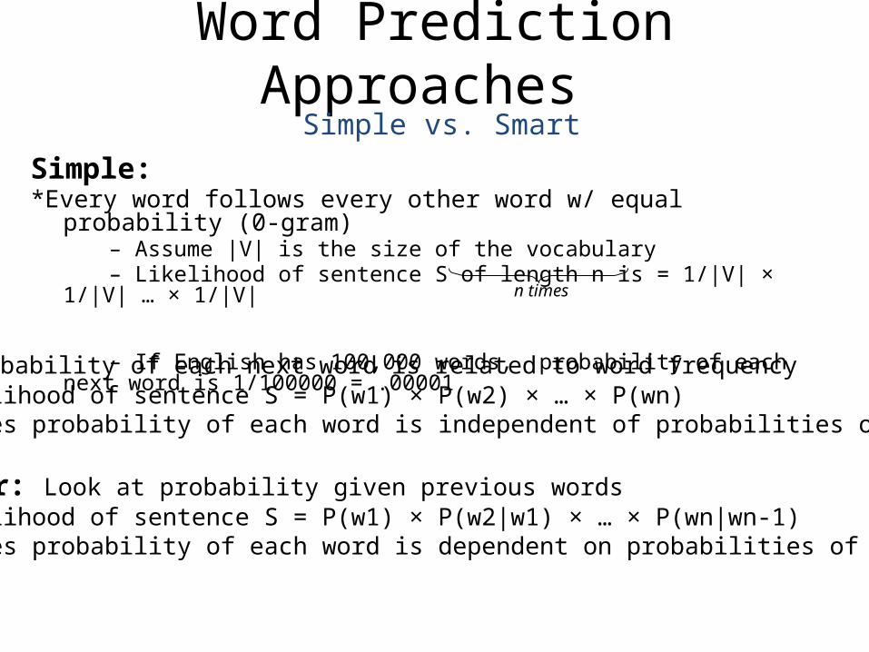
Word Prediction Approaches

Simple:*Every word follows every other word w/ equal probability (0-gram) – Assume |V| is the size of the vocabulary – Likelihood of sentence S of length n is = 1/|V| × 1/|V| … × 1/|V|

– If English has 100,000 words, probability of each next word is 1/100000 = .00001n times

Simple vs. Smart

Smarter: Probability of each next word is related to word frequency – Likelihood of sentence S = P(w1) × P(w2) × … × P(wn) – Assumes probability of each word is independent of probabilities of other words.

Even smarter: Look at probability given previous words – Likelihood of sentence S = P(w1) × P(w2|w1) × … × P(wn|wn-1) – Assumes probability of each word is dependent on probabilities of other words.

Common Spelling Errors

• They are leaving in about fifteen minuets• The study was conducted manly be John Black.• The design an construction of the system will take

more than a year.• Hopefully, all with continue smoothly in my

absence.• Can they lave him my messages?• I need to notified the bank of….• He is trying to fine out.

Spell check without considering context will fail

Difficulty: Detect grammatical errors, or nonsensical expressions

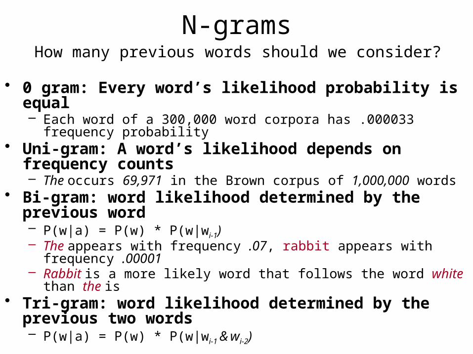
N-grams

• 0 gram: Every word’s likelihood probability is equal– Each word of a 300,000 word corpora has .000033 frequency probability

• Uni-gram: A word’s likelihood depends on frequency counts– The occurs 69,971 in the Brown corpus of 1,000,000 words

• Bi-gram: word likelihood determined by the previous word– P(w|a) = P(w) * P(w|wi-1)– The appears with frequency .07, rabbit appears with frequency .00001– Rabbit is a more likely word that follows the word white than the is

• Tri-gram: word likelihood determined by the previous two words– P(w|a) = P(w) * P(w|wi-1 & wi-2)

• Question: How many previous words should we consider?– Test: Generate random sentences from Shakesphere – Results: Trigram sentences start looking like those of Shakesphere– Tradeoffs: Computational overhead and memory requirements

How many previous words should we consider?

The Sparse Data Problem• Definitions

– Maximum likelihood: Finding the most probable sequence of tokens based on the context of the input

– N-gram sequence: A sequence of n words whose context speech algorithms consider

– Training data: A group of probabilities computed from a corpora of text data

– Sparse data problem: How should algorithms handle n-grams that have very low probabilities?• Data sparseness is a frequently occurring problem• Algorithms will make incorrect decisions if it is not handled

• Problem 1: Low frequency n-grams– Assume n-gram x occurs twice and n-gram y occurs once– Is x really twice as likely to occur as y?

• Problem 2: Zero counts– Probabilities compute to zero for n-grams not seen in the corpora– If n-gram y does not occur, should its probability is zero?

Smoothing

An algorithm that redistributes the probability mass

Discounting: Reduces probabilities of n-grams withnon-zero counts to accommodate the n-grams with zero counts (that are unseen in the corpora).

Definition: A corpora is a collection of written or spoken material in machine-readable form

Add-One Smoothing• The Naïve smoothing technique

– Add one to the count of all seen and unseen n-grams– Add the total increased count to the probability mass

• Example: Uni-grams– Un-smoothed probability for word w: uni-grams

– Add-one revised probability for word w:

– N = number of words encountered, V = vocabulary size, c(w) = number of times word, w, was encountered

P(w) c(w)

N

P1(w) c(w) 1

N V

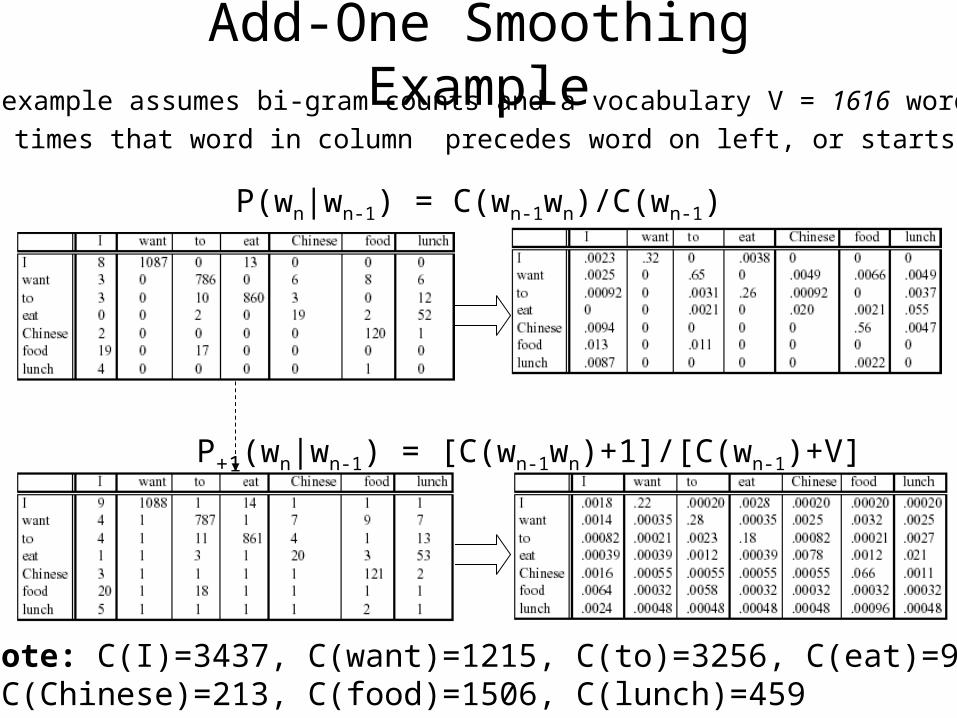
Add-One Smoothing Example

P(wn|wn-1) = C(wn-1wn)/C(wn-1)

P+1(wn|wn-1) = [C(wn-1wn)+1]/[C(wn-1)+V]

Note: This example assumes bi-gram counts and a vocabulary V = 1616 words

Note: row = times that word in column precedes word on left, or starts a sentence

Note: C(I)=3437, C(want)=1215, C(to)=3256, C(eat)=938, C(Chinese)=213, C(food)=1506, C(lunch)=459

Add-One Discounting

VN

N

c’(wi,wi-1) =(c(wi,wi-1)i+1) *

c(wi,wi-1)

Original Counts

Revised Counts

Note: High counts reduce by approximately a third for this example

Note: Low counts get larger

Note: N = c(wi-1), V = vocabulary size = 1616

C(WI)

I 3437

Want 1215

To 3256

Eat 938

Chinese 213

Food 1506

Lunch 459

Evaluation of Add-One Smoothing

• Advantage: – Simple technique to implement and understand

• Disadvantages:– Too much probability mass moves to the unseen n-grams– Underestimates the probabilities of the common n-grams– Overestimates probabilities of rare (or unseen) n-grams– Relative smoothing of all unseen n-grams is the same– Relative smoothing of rare n-grams still incorrect

• Alternative:– Use a smaller add value– Disadvantage: Does not fully solve this problem

Unigram Witten-Bell Discounting

• Compute the probability of a first time encounter of a new word– Note: Every one of O observed words had a first encounter– How many Unseen words: U = V – O – What is the probability of encountering a new word?

• Answer: P( any newly encountered word ) = O/(V+O)• Equally add this probability across all unobserved words

– P( any specific newly encountered word ) = 1/U * O/(V+O)– Adjusted counts = V * 1/U*O/(V+O))

• Discount each encountered wordi to preserve probability space– Probability From: counti /V To: counti/(V+O)– Discounted Counts From: counti To: counti * V/(V+O)

Add probability mass to un-encountered words; discount the rest

O = observed words, U = words never seen, V = corpus vocabulary words

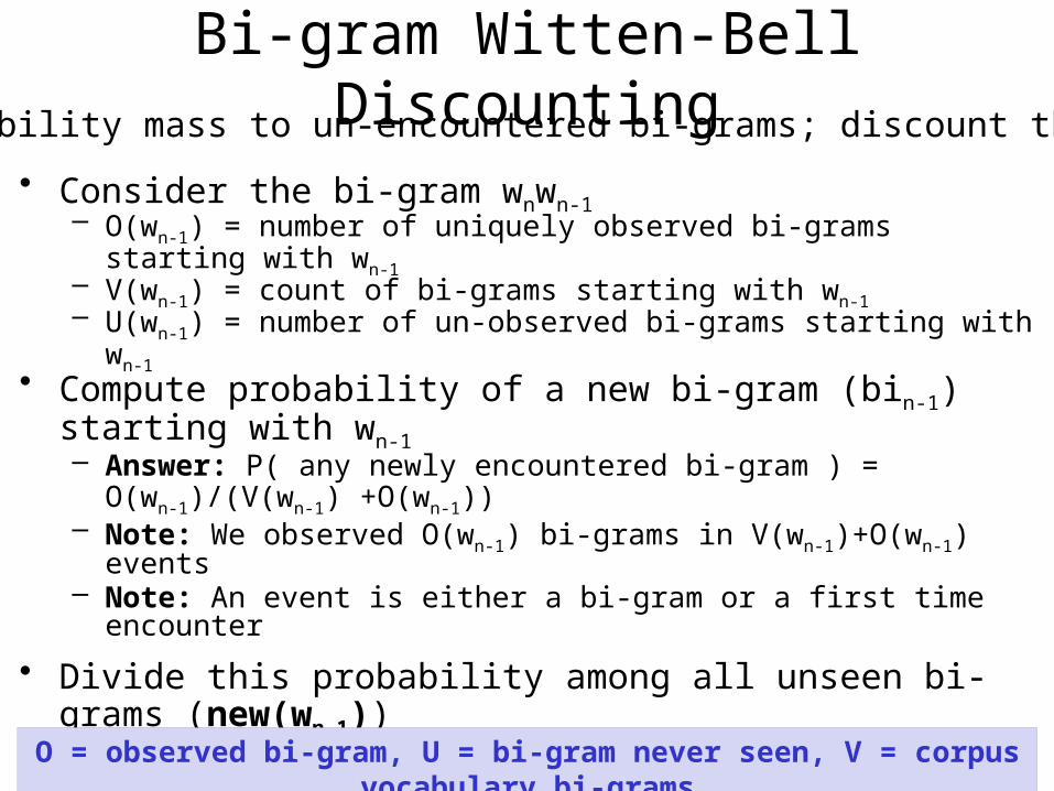
Bi-gram Witten-Bell Discounting

• Consider the bi-gram wnwn-1– O(wn-1) = number of uniquely observed bi-grams starting with wn-1– V(wn-1) = count of bi-grams starting with wn-1– U(wn-1) = number of un-observed bi-grams starting with wn-1• Compute probability of a new bi-gram (bin-1) starting with wn-1– Answer: P( any newly encountered bi-gram ) = O(wn-1)/(V(wn-1) +O(wn-1))– Note: We observed O(wn-1) bi-grams in V(wn-1)+O(wn-1) events– Note: An event is either a bi-gram or a first time encounter

• Divide this probability among all unseen bi-grams (new(wn-1))– Adjusted P(new(wn-1)) = 1/U(wn-1)*O(wn-1)/(V(wn-1)+O(wn-1))– Adjusted count = V(wn-1) * 1/U(wn-1) * O(wn-1)/(V(wn-1)+O(wn-1))

• Discount observed bi-grams gram(wn-1) to preserve probability space– Probability From: c(wn-1 wn)/V(wn-1) To: c(wn-1wn)/(V(wn-1) + O(wn-1))– Counts From: c(wn-1 wn) To: c(wn-1wn) * V(wn-1)/(V(wn-1)+O(wn-1))

Add probability mass to un-encountered bi-grams; discount the rest

O = observed bi-gram, U = bi-gram never seen, V = corpus vocabulary bi-grams

Witten-Bell Smoothing

c′(wn,wn-1)= (c(wn,wn-1)+1)

c(wn,wn-1)

c′(wn,wn-1) = O/U

if c(wn,wn-1)=0

c(wn,wn-1) otherwise

Original Counts

Adjusted Add-One Counts

Adjusted Witten-Bell Counts

V, O and U values are on the next slide

VN

V+

Note: V, O, U refer to wn-1 counts

VNV+

VN

V+

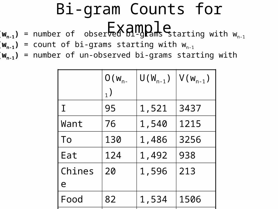
Bi-gram Counts for Example

O(wn-1) U(Wn-1) V(wn-1)

I 95 1,521 3437

Want 76 1,540 1215

To 130 1,486 3256

Eat 124 1,492 938

Chinese 20 1,596 213

Food 82 1,534 1506

Lunch 45 1,571 459

O(wn-1) = number of observed bi-grams starting with wn-1

V(wn-1) = count of bi-grams starting with wn-1 U(wn-1) = number of un-observed bi-grams starting with

Evaluation of Witten-Bell

• Estimates probability of already encountered grams to compute probabilities for unseen grams

• Smaller impact on probabilities of already encountered grams

• Generally computes reasonable probabilities

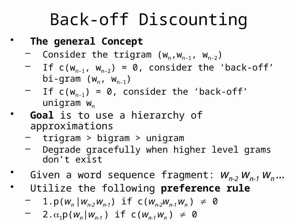
Back-off Discounting• The general Concept

– Consider the trigram (wn,wn-1, wn-2)– If c(wn-1, wn-2) = 0, consider the ‘back-off’ bi-gram (wn, wn-1)– If c(wn-1) = 0, consider the ‘back-off’ unigram wn

• Goal is to use a hierarchy of approximations– trigram > bigram > unigram– Degrade gracefully when higher level grams don’t exist

• Given a word sequence fragment: wn-2 wn-1 wn …• Utilize the following preference rule

– 1.p(wn |wn-2 wn-1) if c(wn-2wn-1 wn ) 0– 2.1p(wn|wn-1 ) if c(wn-1 wn ) 0– 3.2p(wn)

Note: 1 and 2 are values carefully computed to preserve probability mass

N-grams for Spell Checks• Non-word detection (easiest) Example: graffe => (giraffe)

– Isolated-word (context-free) error correction– by definition cannot correct when error word is a valid word

• Context-dependent (hardest) Example: your an idiot => you’re an idiot

• when the mis-typed word happens to be a real word• 15% Peterson (1986), 25%-40% Kukich (1992)