Research ArticleLinear Active Disturbance Rejection Control ofDissolved Oxygen Concentration Based on BenchmarkSimulation Model Number 1
Xiaoyi Wang, Fan Wang, and Wei Wei
School of Computer and Information Engineering, Beijing Technology and Business University, Beijing 100048, China
Correspondence should be addressed to Wei Wei; [email protected]
Received 20 October 2014; Accepted 12 December 2014
Academic Editor: Wudhichai Assawinchaichote
Copyright © 2015 Xiaoyi Wang et al. This is an open access article distributed under the Creative Commons Attribution License,which permits unrestricted use, distribution, and reproduction in any medium, provided the original work is properly cited.
In wastewater treatment plants (WWTPs), the dissolved oxygen is the key variable to be controlled in bioreactors. In this paper,linear active disturbance rejection control (LADRC) is utilized to track the dissolved oxygen concentration based on benchmarksimulation model number 1 (BSM1). Optimal LADRC parameters tuning approach for wastewater treatment processes is obtainedby analyzing and simulations on BSM1. Moreover, by analyzing the estimation capacity of linear extended state observer (LESO)in the control of dissolved oxygen, the parameter range of LESO is acquired, which is a valuable guidance for parameter tuning insimulation and even in practice. The simulation results show that LADRC can overcome the disturbance existing in the control ofwastewater and improve the tracking accuracy of dissolved oxygen. LADRC provides another practical solution to the control ofWWTPs.
1. Introduction
Wastewater treatment plants (WWTPs) are a class of non-linear, uncertain, and time-delay systems. Influent flow rate,contaminant concentrations, amount of pollutants, and otheruncertain factors make the control of wastewater a bigchallenge. Additionally, an increasing discharge standard ofsewage drives people to propose more efficient and practicalapproaches to improve the control of wastewater.
For the control and simulation of WWTPs, in general, amathematical model describing the biochemical process is ofnecessity. Benchmark simulationmodel number 1 (BSM1) hasbeen proposed byWorking Groups of COSTActions 682 and624 [1, 2]. It is a benchmark model for WWTPs with realismand accepted standards. It defines the plant layout, simula-tion, influent loads, test procedures, and evaluation criteria[3–5], and the model could well simulate the main processof wastewater treatment and any control strategy could betested and compared on BSM1. It is a better way to makea simulation study on the control of wastewater treatmentprocess on BSM1.
On BSM1, many manipulated variables, such as thedissolved oxygen concentration, ammonia concentration,
internal recycle flow rate, and external carbon dosing rate [1,2], are involved. BSM1 mainly simulates the activated sludgeprocess. Dissolved oxygen level, a key factor of activatedsludge process, plays a significant role in the behavior of theheterotrophic and autotrophic microorganisms living in theactivated sludge. Proper level of the dissolved oxygen shouldbe supplied for organic matter degradation and nitration;however, excessive dissolved oxygen will increase the pollu-tion concentration and decrease the denitrification process[6–9]. In other words, wastewater effluent quality dependsgreatly on the level of dissolved oxygen.Additionally, effectivecontrol of the dissolved oxygen level could reduce theoperational cost of the wastewater treatment [10]. Therefore,the control of dissolved oxygen concentration is important,effective, and widely studied in WWTPS.
PID is firstly involved in WWTPs for the control ofdissolved oxygen and it is still widely used in practice [11–14].Only 3 parameters and the simple structure make the con-troller easily applied in many occasions. In order to make thedissolved oxygen concentration stably near the expectations,reject disturbances inWWTPs andmake the effluent satisfiedwith the requirements; the proportion parameter of thecontroller has to keep large. However, large proportional
Hindawi Publishing CorporationMathematical Problems in EngineeringVolume 2015, Article ID 178953, 9 pageshttp://dx.doi.org/10.1155/2015/178953

2 Mathematical Problems in Engineering
parameter easily results in high frequency oscillations, whichalso increase the costs or even destabilize the closed-loopsystem. Additionally, all kinds of disturbances existing willdegrade the performance of the closed-loop systems. In thelast decades, various control algorithms have been proposedto control the dissolved oxygen, such as model predictivecontrol (MPC) [7, 10, 15, 16], fuzzy control [6, 17], andneural network control [8, 9, 18, 19]. The MPC has beenwidely applied in industrial processes, especially the fruitfullinear MPC business software packages. However, WWTPsare typical nonlinear systems, and few successful MPCapplications exist in nonlinear systems [20]. Moreover, noclear physical interpretation andhigh amount of computationalways hinder MPC’s applications [20]. Similarly, the fuzzyrules and nonlinear mapping network also require a lotof data for training in fuzzy control and neural networks.In addition, fuzzy rules, the number of nodes of neuralnetworks, and the weight value of neural networks aredifficult to get for achieving good performance.
As a matter of fact, the control of dissolved oxygen inWWTPs is a typical nonlinear and strong couplings process.It is affected by other variables, such as nitrate and nitritenitrogen, ammonia nitrogen, and the internal effluent. If allfactors affecting the control effect of dissolved oxygen can beviewed as disturbances, the core of dissolved oxygen controlis the problem of disturbance rejection.
Linear active disturbance rejection controller (LADRC)is a promising way to solve the disturbance rejection prob-lem. In LADRC structure, the external unknown distur-bance and the internal uncertainty dynamics are treatedas only a generalized disturbance, which can be estimatedand compensated by designing an extended state observerin real time. Therefore, the closed-loop system has greatdisturbance rejection ability. Professor Han firstly proposedactive disturbance rejection control (ADRC), which is takingfull advantage of control errors to suppress the controlerrors [21–23], and it is composed of tracking differentiator(TD), extended state observer (ESO), and nonlinear PID.However, there are 12 parameters in ADRC, which results ina difficult tuning process. With an attempt to simplify thetuning process and make ADRC more practical, LADRC isproposed with linearizing the ESO and TD by Gao in 2003.By this simplification, LADRC only has 3 parameters fortuning [24]. LADRC has lots of successful applications [25–28]. Simulation and experimental results prove that LADRChas nice performance and strong robustness to disturbances.In WWTPs, the variables except the dissolved oxygen canbe regarded as the internal uncertain dynamics, while theinfluent can be regarded as the external unknown distur-bance, which could be estimated and compensated by thelinear extended state observer (LESO). Therefore, LADRCmay have good effect in the control of dissolved oxygen.However, the ability of LADRC to overcome the disturbanceof WWTPs and how to choose proper LADRC parametersfor the control of dissolved oxygen are unclear. Both of themare worth making a further research in theory and practicefor WWTPs. For this purpose, some theoretical analysis andsimulation researches are fulfilled.
This paper is organized as follows. Section 2 presentsthe basic structure of BSM1, the dissolved oxygen controlstrategy, and the design approaches of LADRC. Section 3presents the results of simulation, the steps of parameterstuning, and related analysis. Finally, conclusions are given inSection 4.
2. Benchmark Simulation Model Number 1and Its Control Strategy
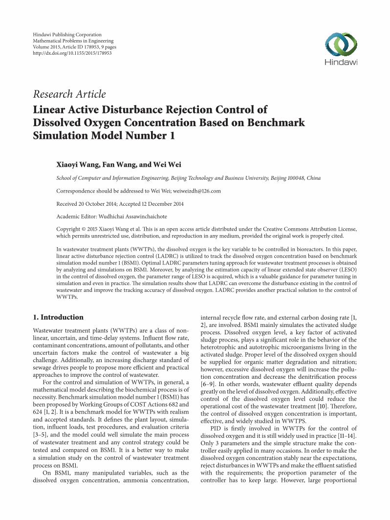
2.1. The BSM1 Introduction. BSM1 layout can be divided intotwo parts, which includes 5 activated sludge reactors anda secondary settler. General structure of BSM1 is shown inFigure 1. Five activated sludge reactors are called bioreactorswhich are composed of 2 anoxic tanks (Units 1 and 2) and3 aerobic tanks (Units 3–5). The activated sludge modelnumber 1 (ASM1) has been selected to describe the biologicalphenomena taking place in biological reactors [29, 30].Thus,the model includes oxidizing reactions, nitrification, anddenitrification for removing biological nitrogen. Behind thereactors, there is a secondary settler, which is composed of10 layers. The 6th layer is the feed layer, through which thewastewater is from the bioreactors to the secondary settler.At last the treated wastewater comes out of the 10th layer andparts of the sludge from the 1st layer go back toUnit 1 throughthe external recycle. In the secondary settler, there is nobiochemical reaction, just physical deposition. The double-exponential settling velocity function has been selected todescribe the secondary settler [31, 32].
In ASM1, there are 13 state variables (including 6 par-ticulate components and 7 soluble components), 8 basicprocesses, 5 stoichiometric parameters, and 14 kinetic param-eters. All the variables, processes, andparameters describe theoxidizing reactions, nitration reactions, and denitrificationreactions. Reactions in each bioreactor about 13 state vari-ables follow mass balancing:
𝑑𝑍𝑘
𝑑𝑡=1
𝑉𝑘
(𝑄𝑘−1𝑍𝑘−1 − 𝑟𝑖𝑉𝑘 − 𝑄𝑘𝑍𝑘) , (1)
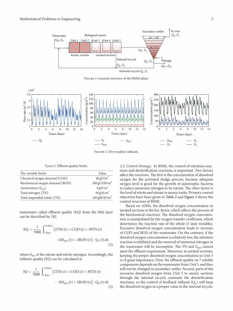
where 𝑘 is the bioreactor number, 𝑍𝑘 is the state variables,𝑄𝑘 is the influent, 𝑉𝑘 is the volume of the bioreactor, 𝑟𝑖 is theobserved conversion rates, and 𝑖 is from 1 to 13. 𝑟𝑖 is the coreparameter in ASM1, which reflects the relationship amongvariables. BSM1 is built with Matlab/Simulink, including 5bioreactors, a secondary settler, and a time-delay unit. Thesimulation data of dry weather, rainy weather, and stormyweather on benchmark of WWTPs on 14 days is provided totest the model. Only the dry weather data present in Figure 2is used in this paper, because the data of dry weather, rainyweather, and stormy weather is the same except the last 2 twodays.
The flow-weighted average values of the effluent con-centrations, such as chemical oxygen demand (COD), bio-chemical oxygen demand (BOD), ammonium (𝑆NH), totalnitrogen (TN), and total suspended solids (TSS) [1, 2], shouldbe within the limits given in Table 1. The quality of processed
Mathematical Problems in Engineering 3
Biological reactorWastewater
Anoxic section Aerated section
WastageInternal recycle
To river
Unit 1 Unit 2 Unit 3 Unit 4 Unit 5Q0, Z0
Qa, Za QW, ZW
Qe, Ze
Qr, ZrExternal recycle
Qu, Zu
Qf, Zf
m = 10
m = 6
m = 1
Secondary settler
Figure 1: General overview of the BSM1 plant.
0 2 4 6 8 10 12 141
1.5
2
2.5
3
3.5
Times (days)
020406080
100120140
Times (days)
0
50
100
150
200
250
300×104
Flow
rate
(m3/d
)
Con
cent
ratio
n (g
/m3)
Con
cent
ratio
n (g
/m3)
SSSNH
SND XBHXS XS
XiQa
0 2 4 6 8 10 12 14Times (days)
0 2 4 6 8 10 12 14
Figure 2: Dry weather influent.
Table 1: Effluent quality limits.
The variable limits ValueChemical oxygen demand (COD) 18 gN/m3
Biochemical oxygen demand (BOD) 100 gCOD/m3
Ammonium (𝑆NH) 4 gN/m3
Total nitrogen (TN). 30 gSS/m3
Total suspended solids (TSS) 100 gBOD/m3
wastewater called effluent quality (EQ) from the 10th layercan be described by [31]
EQ =1
7000∫
14 days
7 days[2TSS (𝑡) + COD (𝑡) + 30TN (𝑡)
−20𝑆NO (𝑡) + 2BOD (𝑡)] ⋅ 𝑄𝑒 (𝑡) 𝑑𝑡,(2)
where 𝑆NO is the nitrate and nitrite nitrogen. Accordingly, theinfluent quality (IQ) can be calculated as
IQ =1
7000∫
14 days
7 days[2TSS (𝑡) + COD (𝑡) + 30TN (𝑡)
− 20𝑆NO (𝑡) + 2BOD (𝑡)] ⋅ 𝑄0 (𝑡) 𝑑𝑡.(3)
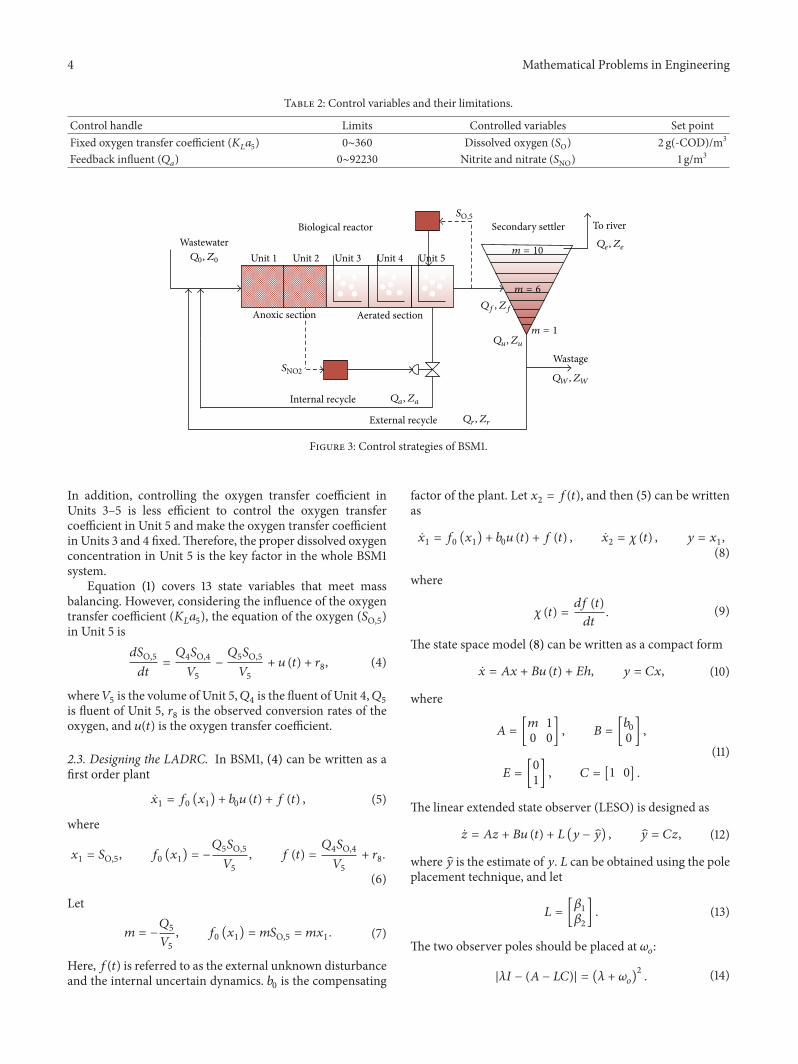
2.2. Control Strategy. In BSM1, the control of nitration reac-tions and denitrification reactions is important. Two factorsaffect the reactions.The first is the concentration of dissolvedoxygen for the activated sludge process, because adequateoxygen level is good for the growth of autotrophic bacteriato reduce ammonia nitrogen to be nitrate. The other factor isthe level of nitrite and nitrate in anoxic tanks. Primary controlobjectives have been given in Table 2 and Figure 3 shows thecontrol structure of BSM1.
Based on ASM1, the dissolved oxygen concentration inaerated sections is the key factor, which affects the process ofthe biochemical reactions. The dissolved oxygen concentra-tion is manipulated by the oxygen transfer coefficient, whichdetermines the reaction rate of the whole 13 state variables.Excessive dissolved oxygen concentration leads to increaseof COD and BOD of the wastewater. On the contrary, if thedissolved oxygen concentration is relatively low, the nitrationreaction is inhibited and the removal of ammonia nitrogen inthe wastewater will be incomplete. The TN and 𝑆NH cannotmeet the effluent requirement. Moreover, in aerated sections,keeping the proper dissolved oxygen concentration in Unit 5is of great importance. First, the effluent quality on 7 solublecomponents depends on thewastewater fromUnit 5, and theywill not be changed in secondary settler. Second, parts of theexcessive dissolved oxygen from Unit 5 to anoxic sectionsthrough the internal recycle constrain the denitrificationreactions, so the control of feedback influent (𝑄𝑎) will keepthe dissolved oxygen in a proper value in the internal recycle.
4 Mathematical Problems in Engineering
Table 2: Control variables and their limitations.
Control handle Limits Controlled variables Set pointFixed oxygen transfer coefficient (𝐾𝐿𝑎5) 0∼360 Dissolved oxygen (𝑆O) 2 g(-COD)/m3
Feedback influent (𝑄𝑎) 0∼92230 Nitrite and nitrate (𝑆NO) 1 g/m3
Biological reactor
Anoxic section Aerated section
Wastage
Internal recycle
External recycle
Secondary settler To river
Unit 1 Unit 2 Unit 3 Unit 4 Unit 5Wastewater
Q0, Z0
Qa, Za
Qr, Zr
SNO2
Qe, Ze
QW, ZW
Qu, Zu
Qf, Zf
m = 10
m = 6
m = 1
SO,5
Figure 3: Control strategies of BSM1.
In addition, controlling the oxygen transfer coefficient inUnits 3–5 is less efficient to control the oxygen transfercoefficient in Unit 5 and make the oxygen transfer coefficientin Units 3 and 4 fixed.Therefore, the proper dissolved oxygenconcentration in Unit 5 is the key factor in the whole BSM1system.
Equation (1) covers 13 state variables that meet massbalancing. However, considering the influence of the oxygentransfer coefficient (𝐾𝐿𝑎5), the equation of the oxygen (𝑆O,5)in Unit 5 is
𝑑𝑆O,5
𝑑𝑡=𝑄4𝑆O,4
𝑉5
−𝑄5𝑆O,5
𝑉5
+ 𝑢 (𝑡) + 𝑟8, (4)
where𝑉5 is the volume of Unit 5,𝑄4 is the fluent of Unit 4,𝑄5is fluent of Unit 5, 𝑟8 is the observed conversion rates of theoxygen, and 𝑢(𝑡) is the oxygen transfer coefficient.
2.3. Designing the LADRC. In BSM1, (4) can be written as afirst order plant
��1 = 𝑓0 (𝑥1) + 𝑏0𝑢 (𝑡) + 𝑓 (𝑡) , (5)
where
𝑥1 = 𝑆O,5, 𝑓0 (𝑥1) = −𝑄5𝑆O,5
𝑉5
, 𝑓 (𝑡) =𝑄4𝑆O,4
𝑉5
+ 𝑟8.
(6)
Let
𝑚 = −𝑄5
𝑉5
, 𝑓0 (𝑥1) = 𝑚𝑆O,5 = 𝑚𝑥1. (7)
Here, 𝑓(𝑡) is referred to as the external unknown disturbanceand the internal uncertain dynamics. 𝑏0 is the compensating
factor of the plant. Let 𝑥2 = 𝑓(𝑡), and then (5) can be writtenas
��1 = 𝑓0 (𝑥1) + 𝑏0𝑢 (𝑡) + 𝑓 (𝑡) , ��2 = 𝜒 (𝑡) , 𝑦 = 𝑥1,
(8)
where
𝜒 (𝑡) =𝑑𝑓 (𝑡)
𝑑𝑡. (9)
The state space model (8) can be written as a compact form
�� = 𝐴𝑥 + 𝐵𝑢 (𝑡) + 𝐸ℎ, 𝑦 = 𝐶𝑥, (10)
where
𝐴 = [𝑚 1
0 0] , 𝐵 = [
𝑏00] ,
𝐸 = [0
1] , 𝐶 = [1 0] .
(11)
The linear extended state observer (LESO) is designed as
�� = 𝐴𝑧 + 𝐵𝑢 (𝑡) + 𝐿 (𝑦 − 𝑦) , 𝑦 = 𝐶𝑧, (12)
where 𝑦 is the estimate of 𝑦. 𝐿 can be obtained using the poleplacement technique, and let
𝐿 = [𝛽1𝛽2] . (13)
The two observer poles should be placed at 𝜔𝑜:
|𝜆𝐼 − (𝐴 − 𝐿𝐶)| = (𝜆 + 𝜔𝑜)2. (14)

Mathematical Problems in Engineering 5
LESO
LADRC
r𝜔c 1/b0 BSM1
KLa5 yu
+
−
+
−
SO,5
Figure 4: Control scheme of dissolved oxygen on BSM1.
Then, 𝛽1 and 𝛽2 can be placed at 2𝜔𝑜 + 𝑚 and 𝜔2𝑜. Therefore,
LESO is
�� = [−2𝜔𝑜 1
−𝜔2
𝑜0] 𝑧 + [
𝑏00] 𝑢 (𝑡) + [
2𝜔𝑜 + 𝑚
𝜔2
𝑜
] 𝑦. (15)
The PD controller is
𝑢 (𝑡) =(𝑟 − 𝑧1) 𝑘𝑑 − 𝑧2
𝑏0
, (16)
where the gain 𝑘𝑑 can be defined as the function of closed-loop natural frequency 𝜔𝑐 [24]. The control scheme ofdissolved oxygen in BSM1 by LADRC is given in Figure 4.
3. Simulation Results and Discussions
3.1. LADRC Parameter Tuning. In (15) and (16), 3 parameters,𝜔𝑜, 𝜔𝑐, and 𝑏0, are tunable parameters of LADRC. Integralof absolute error (IAE), integral of squared error (ISE), andvariance of error (VAR) are calculated to evaluate the controlof LADRConBSM1 [2].The optimal LADRC tuning steps aregiven below.
Step 1. In (4) and (5), 𝑏0 can be set to be 1 (if the plant isunknown, 𝑏0 could be acquired by simulation).
Step 2. A common rule is to choose 𝜔𝑜 = 3 ∼ 5𝜔𝑐 [24]. Basedon this rule, we may get a set of 𝜔𝑐 and 𝜔𝑜 that can stabilizethe systems.
(a) Fixing 𝜔𝑐, increasing and decreasing 𝜔𝑜, we can findseveral groups of stable parameters named class A.
(b) Fixing 𝜔𝑜, increasing and decreasing 𝜔𝑐, we can findanother class B.
(c) Comparing A and B, we may find the relationshipbetween 𝜔𝑜 and 𝜔𝑐.
(d) Changing both𝜔𝑐 and𝜔𝑜 on this relationship, wemayfind other groups of stable parameters.
Step 3. By comparison with the value of IAE, ISE, and VAR,optimal parameters can be found easily.
According to the steps described above, several groups ofsimulation are performed, and several results can be found.
(1) Dissolved oxygen concentration in Unit 5 could keepnear 2g(-COD)/m3 (see Figure 5(a)) when nearly𝜔𝑜+𝜔𝑐 = 1000, 𝜔𝑐 > 40, and 𝜔𝑜 < 900.
(2) If𝜔𝑜 < 200, the concentration of the dissolved oxygenfluctuates greatly (see Figure 5(b)).
(3) If 𝜔𝑜 ≥ 900, the disturbance is larger than thecontrolled signal. Performance of the closed-loopsystem degrades (see Figure 5(c)).
(4) If 𝜔𝑜 is decreased, 𝜔𝑐 must be increased to keep theperformance (see Table 3).
Parts of simulation results are present in Figure 5. Theperformance of closed-loop system and the EQ values areshown in Table 3. Comparing groups a ∼ j, one may find thatas long as the dissolved oxygen concentration in Unit 5 keepsnear 2g(-COD)/m3, the EQ values are almost the same.
In Table 3, the optimal parameters are shown in group e.In fact, the performances of the groups c ∼ h look the samein Figure 5. When the parameters are chosen as group e,the variation of 𝑆O,5 and 𝐾𝐿𝑎5 is shown in Figure 6, whichgives out the comparison with virtual reference feedbacktuning (VRFT) [19]. The change of wastewater quality isgiven in Table 4. Apparently, the wastewater quality has beenimproved greatly.
3.2. Analysis of LADRC Parameters to BSM1. In Section 2.3,LADRC is designed based on BSM1. LESO is the key part ofLADRC, which can actively estimate two states, 𝑦 and 𝑓(𝑡).The estimation errors 𝑒1 and 𝑒2 can be defined by
𝑒1 = 𝑧1 − 𝑦 = 𝑧1 − 𝑥1,
𝑒2 = 𝑧2 − 𝑓 (𝑡) = 𝑧2 − 𝑥2.
(17)
According to (12) and (13), LESO can be rewritten as
��1 = 𝑚𝑧1 + 𝑧2 − 𝛽1 (𝑧1 − 𝑦) + 𝑏0𝑢 (𝑡)
= 𝑚𝑧1 + 𝑧2 − 𝛽1𝑒1 + 𝑏0𝑢 (𝑡) ,
��2 = −𝛽2𝑒1.
(18)
Then, the differential errors are
𝑒1 = 𝑒2 − (𝛽1 − 𝑚) 𝑒1, 𝑒2 = −𝜒 (𝑡) − 𝛽2𝑒1. (19)
When the states go into steady, that is 𝑒1 and 𝑒2 are almostzero, we have,
𝑒2 − (𝛽1 − 𝑚) 𝑒1 = 0, −𝜒 (𝑡) − 𝛽2𝑒1 = 0. (20)
The errors are obtained as
𝑒1 = −𝜒 (𝑡)
𝛽2
, 𝑒2 = (𝛽1 − 𝑚) 𝑒1 (21)
which can be rewritten as
𝑒1 = −𝜒 (𝑡)
𝜔2𝑜
, 𝑒2 = 2𝜔2
𝑜𝑒1, (22)
where𝛽1 = 2𝜔𝑜+𝑚 and𝛽2 = 𝜔2
𝑜. If𝜔2𝑜≫ −𝜒(𝑡), 𝑒1 will tend to
zero and 𝑒2 will also tend to zero. In other words, LESO could

6 Mathematical Problems in Engineering
0 2 4 6 8 10 12 141.5
1.75
2
2.25
2.5
Times (days)
cde
fgh
S O(g
/m−3)
(a)
Times (days)0 2 4 6 8 10 12 14
1.5
1.75
2
2.25
2.5
hij
S O(g
/m−3)
(b)
0 2 4 6 8 10 12 141.5
1.75
2
2.25
2.5
ab
Times (days)
S O(g
/m−3)
(c)
Figure 5: Comparison of the dissolved oxygen concentration in Unit 5 for different LADRC parameters.
7 8 9 10 11 12 13 141
1.2
1.4
1.6
1.8
2
2.2
2.4
2.6
2.8
3
Times (days) Times (days)
VRFTLADRC
VRFTLADRC
7 8 9 10 11 12 13 140
50
100
150
200
250
300
KLa 5
(1/d
)
(g/m
3)
S O,5
Figure 6: Comparison of 𝑆O,5 and 𝐾𝐿𝑎5 for VRFT and LADRC.

Mathematical Problems in Engineering 7
Table 3: Performance indexes of the closed-loop system.
𝑏0
𝜔𝑐
𝜔𝑜
IAE ISE VAR EQa 1 50 950 0.818 0.198 0.01080 6155.0
b 1 100 900 0.085 0.242 0.001700 6153.9
c 1 200 800 0.051 0.012 0.00089 6153.7
d 1 300 700 0.056 0.007 0.00050 6154.1
e 1 400 600 0.037 0.006 0.00039 6154.1
f 1 500 500 0.385 0.004 0.00030 6153.9
g 1 600 400 0.454 0.004 0.00028 6154.1
h 1 700 300 0.615 0.005 0.00028 6154.2
i 1 800 200 0.107 0.006 0.00035 6153.9
j 1 900 100 0.328 0.023 0.00110 6154.8
Table 4: Comparison of influent and effluent.
Standers Influent EffluentNT 51.47 17.39
COD 360.04 46.58
𝑆NH 30.14 2.61
BOD 183.51 2.58
TSS 198.60 11.73
IQ/EQ 52089 6154.12
estimate the 𝑦 and 𝑓(𝑡) effectively. From Section 2.3, 𝑓(𝑡) canbe described by
𝑓 (𝑡) =𝑄4𝑆O,4
𝑉5
+ 𝑟8 =𝑄4𝑆O,4
𝑉5
−1 − 𝑌𝐻
𝑌𝐻
𝜌1
−4.75 − 𝑌𝐴
𝑌𝐴
𝜌3,
(23)
where 𝑌𝐻 and 𝑌𝐴 are the parameters of BSM1, 𝜌1 is the basicprocess of aerobic growth of heterotrophs, and 𝜌3 is the basicprocess of aerobic growth of autotrophs:
𝜌1 =4𝑆S,5
𝑆S,5 + 10
𝑆O,5
𝑆O,5 + 0.2𝑋BH,5
𝜌3 =0.5𝑆NH,5
𝑆NH,5 + 1
𝑆O,5
𝑆O,5 + 0.4𝑋BA,5,
(24)
where 𝑆S,5 is the readily biodegradable substrate in Unit 5,𝑋BH,5 is the active heterotrophic biomass in Unit 5, 𝑆NH,5 isthe nitrogen in Unit 5, and 𝑋BA,5 is the active autotrophicbiomass. Then the differential of 𝑓(𝑡) is
𝜒 (𝑡) =𝑑𝑓 (𝑡)
𝑑𝑡=𝑄4
𝑉5
𝑑𝑆O,4
𝑑𝑡−1 − 𝑌𝐻
𝑌𝐻
𝑑𝜌1
𝑑𝑡−4.75 − 𝑌𝐴
𝑌𝐴
𝑑𝜌3
𝑑𝑡,
(25)
0 2 4 6 8 10 12 14
0
Times (days)
−4
−3.5
−3
−2.5
−2
−1.5
−1
−0.5
×104
𝜒(t)
Figure 7: Estimate of 𝜒(𝑡).
where
𝑑𝜌1
𝑑𝑡=
4𝑆O,5
𝑆O,5 + 0.2[10𝑋BH,5 (𝑑𝑆S,5/𝑑𝑡)
(𝑆S,5 + 10)2
+𝑆S,5
𝑆S,5 + 10
𝑑𝑋BH,5
𝑑𝑡] ,
𝑑𝜌3
𝑑𝑡=
0.5𝑆O,5
𝑆O,5 + 0.4[𝑋BA,5 (𝑑𝑆NH,5/𝑑𝑡)
(𝑆NH,5 + 1)2
+𝑆NH,5
𝑆NH,5 + 1
𝑑𝑋BA,5
𝑑𝑡] .
(26)
𝜌1 and 𝜌3 include the controlled state variable 𝑆O,5. For thewastewater process being a large time-delay system, it isreasonable to let 𝑆O,5 in 𝜒(𝑡) be a small variable in [2 −
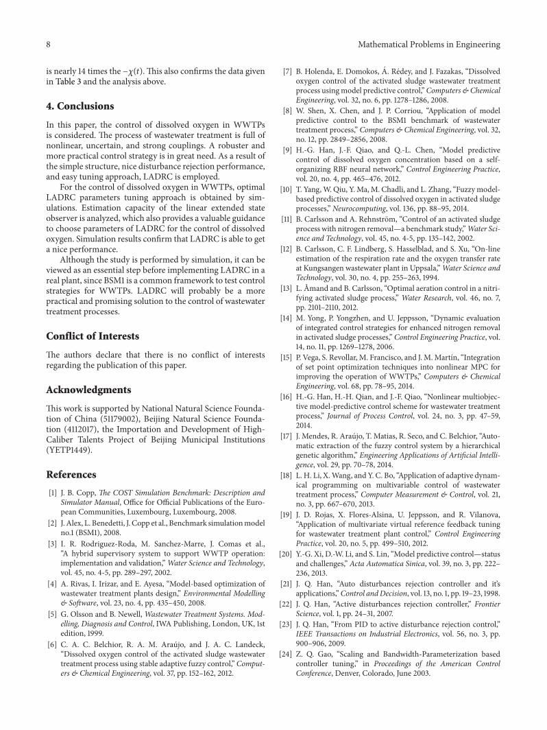
Δ, 2 + Δ], where Δ leads to zero. At the same time, anothervariable could be estimated by a 14-day period of stabilizationin closed-loop using dry weather inputs [4]. Through thesimulation and calculation, 𝜒(𝑡) is described in Figure 7 withΔ about 0.2.
If the parameter 𝜔𝑜 meets 𝜔2𝑜≫ −𝜒(𝑡), 𝜔𝑜 should exceed
160. In Section 3.1, if the parameter 𝜔𝑜 < 200, the fluctuate ofthe dissolved oxygen concentration becomes large.Therefore,the optimal parameters are 𝜔𝑜 = 600 and 𝜔𝑐 = 400. This 𝜔2
𝑜
8 Mathematical Problems in Engineering
is nearly 14 times the −𝜒(𝑡). This also confirms the data givenin Table 3 and the analysis above.
4. Conclusions
In this paper, the control of dissolved oxygen in WWTPsis considered. The process of wastewater treatment is full ofnonlinear, uncertain, and strong couplings. A robuster andmore practical control strategy is in great need. As a result ofthe simple structure, nice disturbance rejection performance,and easy tuning approach, LADRC is employed.
For the control of dissolved oxygen in WWTPs, optimalLADRC parameters tuning approach is obtained by sim-ulations. Estimation capacity of the linear extended stateobserver is analyzed, which also provides a valuable guidanceto choose parameters of LADRC for the control of dissolvedoxygen. Simulation results confirm that LADRC is able to geta nice performance.
Although the study is performed by simulation, it can beviewed as an essential step before implementing LADRC in areal plant, since BSM1 is a common framework to test controlstrategies for WWTPs. LADRC will probably be a morepractical and promising solution to the control of wastewatertreatment processes.
Conflict of Interests
The authors declare that there is no conflict of interestsregarding the publication of this paper.
Acknowledgments
This work is supported by National Natural Science Founda-tion of China (51179002), Beijing Natural Science Founda-tion (4112017), the Importation and Development of High-Caliber Talents Project of Beijing Municipal Institutions(YETP1449).
References
[1] J. B. Copp, The COST Simulation Benchmark: Description andSimulator Manual, Office for Official Publications of the Euro-pean Communities, Luxembourg, Luxembourg, 2008.
[2] J. Alex, L. Benedetti, J. Copp et al., Benchmark simulationmodelno.1 (BSM1), 2008.
[3] I. R. Rodriguez-Roda, M. Sanchez-Marre, J. Comas et al.,“A hybrid supervisory system to support WWTP operation:implementation and validation,”Water Science and Technology,vol. 45, no. 4-5, pp. 289–297, 2002.
[4] A. Rivas, I. Irizar, and E. Ayesa, “Model-based optimization ofwastewater treatment plants design,” Environmental Modelling& Software, vol. 23, no. 4, pp. 435–450, 2008.
[5] G. Olsson and B. Newell,Wastewater Treatment Systems. Mod-elling, Diagnosis and Control, IWA Publishing, London, UK, 1stedition, 1999.
[6] C. A. C. Belchior, R. A. M. Araujo, and J. A. C. Landeck,“Dissolved oxygen control of the activated sludge wastewatertreatment process using stable adaptive fuzzy control,” Comput-ers & Chemical Engineering, vol. 37, pp. 152–162, 2012.
[7] B. Holenda, E. Domokos, A. Redey, and J. Fazakas, “Dissolvedoxygen control of the activated sludge wastewater treatmentprocess usingmodel predictive control,”Computers & ChemicalEngineering, vol. 32, no. 6, pp. 1278–1286, 2008.
[8] W. Shen, X. Chen, and J. P. Corriou, “Application of modelpredictive control to the BSM1 benchmark of wastewatertreatment process,” Computers & Chemical Engineering, vol. 32,no. 12, pp. 2849–2856, 2008.
[9] H.-G. Han, J.-F. Qiao, and Q.-L. Chen, “Model predictivecontrol of dissolved oxygen concentration based on a self-organizing RBF neural network,” Control Engineering Practice,vol. 20, no. 4, pp. 465–476, 2012.
[10] T. Yang,W. Qiu, Y.Ma,M. Chadli, and L. Zhang, “Fuzzymodel-based predictive control of dissolved oxygen in activated sludgeprocesses,” Neurocomputing, vol. 136, pp. 88–95, 2014.
[11] B. Carlsson and A. Rehnstrom, “Control of an activated sludgeprocess with nitrogen removal—a benchmark study,”Water Sci-ence and Technology, vol. 45, no. 4-5, pp. 135–142, 2002.
[12] B. Carlsson, C. F. Lindberg, S. Hasselblad, and S. Xu, “On-lineestimation of the respiration rate and the oxygen transfer rateat Kungsangen wastewater plant in Uppsala,”Water Science andTechnology, vol. 30, no. 4, pp. 255–263, 1994.
[13] L. Amand and B. Carlsson, “Optimal aeration control in a nitri-fying activated sludge process,” Water Research, vol. 46, no. 7,pp. 2101–2110, 2012.
[14] M. Yong, P. Yongzhen, and U. Jeppsson, “Dynamic evaluationof integrated control strategies for enhanced nitrogen removalin activated sludge processes,” Control Engineering Practice, vol.14, no. 11, pp. 1269–1278, 2006.
[15] P. Vega, S. Revollar, M. Francisco, and J.M.Martın, “Integrationof set point optimization techniques into nonlinear MPC forimproving the operation of WWTPs,” Computers & ChemicalEngineering, vol. 68, pp. 78–95, 2014.
[16] H.-G. Han, H.-H. Qian, and J.-F. Qiao, “Nonlinear multiobjec-tive model-predictive control scheme for wastewater treatmentprocess,” Journal of Process Control, vol. 24, no. 3, pp. 47–59,2014.
[17] J. Mendes, R. Araujo, T. Matias, R. Seco, and C. Belchior, “Auto-matic extraction of the fuzzy control system by a hierarchicalgenetic algorithm,” Engineering Applications of Artificial Intelli-gence, vol. 29, pp. 70–78, 2014.
[18] L. H. Li, X.Wang, and Y. C. Bo, “Application of adaptive dynam-ical programming on multivariable control of wastewatertreatment process,” Computer Measurement & Control, vol. 21,no. 3, pp. 667–670, 2013.
[19] J. D. Rojas, X. Flores-Alsina, U. Jeppsson, and R. Vilanova,“Application of multivariate virtual reference feedback tuningfor wastewater treatment plant control,” Control EngineeringPractice, vol. 20, no. 5, pp. 499–510, 2012.
[20] Y.-G. Xi, D.-W. Li, and S. Lin, “Model predictive control—statusand challenges,” Acta Automatica Sinica, vol. 39, no. 3, pp. 222–236, 2013.
[21] J. Q. Han, “Auto disturbances rejection controller and it’sapplications,”Control andDecision, vol. 13, no. 1, pp. 19–23, 1998.
[22] J. Q. Han, “Active disturbances rejection controller,” FrontierScience, vol. 1, pp. 24–31, 2007.
[23] J. Q. Han, “From PID to active disturbance rejection control,”IEEE Transactions on Industrial Electronics, vol. 56, no. 3, pp.900–906, 2009.
[24] Z. Q. Gao, “Scaling and Bandwidth-Parameterization basedcontroller tuning,” in Proceedings of the American ControlConference, Denver, Colorado, June 2003.

Mathematical Problems in Engineering 9
[25] Y.-C. Fang, H. Shen, X.-Y. Sun, X. Zhang, and B. Xian,“Active disturbance rejection control for heading of unmannedhelicopter,”ControlTheory&Applications, vol. 31, no. 2, pp. 238–243, 2014.
[26] C.-E. Huang, D. Li, and Y. Xue, “Active disturbance rejectioncontrol for the ALSTOM gasifier benchmark problem,” ControlEngineering Practice, vol. 21, no. 4, pp. 556–564, 2013.
[27] A. Rodriguez-Angeles and J. A. Garcia-Antonio, “Active distur-bance rejection control in steering by wire haptic systems,” ISATransactions, vol. 53, no. 4, pp. 939–946, 2014.
[28] L. Fucai, L. Lihuan, G. Juanjuan, and G. Wenkui, “Activedisturbance rejection trajectory tracking control for spacemanipulator in different gravity environment,” Control Theory& Applications, vol. 31, no. 3, pp. 352–360, 2014.
[29] M. Henze, W. Gujer, T. Mino et al., “Activated sludge modelno.1,” IAWPRC Scientific and Technical Reports 1, 1986.
[30] M. Henze, W. Gujer, T. Mino, and M. van Loosdrecht, Eds.,Activated Sludge Models ASM1, ASM2, ASM2d and ASM3, IWAPublishing, IWA Task Group on Mathematical Modelling forDesign and Operation of Biological Wastewater Treatment,London, UK, 2004.
[31] I. Takacs, G. G. Patry, and D. Nolasco, “A dynamic model of theclarification-thickening process,”Water Research, vol. 25, no. 10,pp. 1263–1271, 1991.
[32] TheEuropean cooperation in the field of scientific and technicalresearch, Action 624: Optimal Management of WastewaterSystems, http://apps.ensic.inpl-nancy.fr/COSTWWTP/.

Submit your manuscripts athttp://www.hindawi.com
Hindawi Publishing Corporationhttp://www.hindawi.com Volume 2014
MathematicsJournal of
Hindawi Publishing Corporationhttp://www.hindawi.com Volume 2014
Mathematical Problems in Engineering
Hindawi Publishing Corporationhttp://www.hindawi.com
Differential EquationsInternational Journal of
Volume 2014
Applied MathematicsJournal of
Hindawi Publishing Corporationhttp://www.hindawi.com Volume 2014
Probability and StatisticsHindawi Publishing Corporationhttp://www.hindawi.com Volume 2014
Journal of
Hindawi Publishing Corporationhttp://www.hindawi.com Volume 2014
Mathematical PhysicsAdvances in
Complex AnalysisJournal of
Hindawi Publishing Corporationhttp://www.hindawi.com Volume 2014
OptimizationJournal of
Hindawi Publishing Corporationhttp://www.hindawi.com Volume 2014
CombinatoricsHindawi Publishing Corporationhttp://www.hindawi.com Volume 2014
International Journal of
Hindawi Publishing Corporationhttp://www.hindawi.com Volume 2014
Operations ResearchAdvances in
Journal of
Hindawi Publishing Corporationhttp://www.hindawi.com Volume 2014
Function Spaces
Abstract and Applied AnalysisHindawi Publishing Corporationhttp://www.hindawi.com Volume 2014
International Journal of Mathematics and Mathematical Sciences
Hindawi Publishing Corporationhttp://www.hindawi.com Volume 2014
The Scientific World JournalHindawi Publishing Corporation http://www.hindawi.com Volume 2014
Hindawi Publishing Corporationhttp://www.hindawi.com Volume 2014
Algebra
Discrete Dynamics in Nature and Society
Hindawi Publishing Corporationhttp://www.hindawi.com Volume 2014
Hindawi Publishing Corporationhttp://www.hindawi.com Volume 2014
Decision SciencesAdvances in
Discrete MathematicsJournal of
Hindawi Publishing Corporationhttp://www.hindawi.com
Volume 2014 Hindawi Publishing Corporationhttp://www.hindawi.com Volume 2014
Stochastic AnalysisInternational Journal of
Recommended