Reprocessing GPS dataat the observation level

for tide gauge monitoring:

G. Wöppelmann, Tilo Schöne

IGS Analysis Center Workshop 2008, 2-6 June 2008, Miami Beach, Florida, USA

Main “raison d’être” of TIGA

I. What are the sea-level applications requirements?

II. The TIGA Pilot Project III. An example: Reprocessing Strategy at ULR IV. Some important issues to do with cGPS@TG

V. Outlooks

Overview

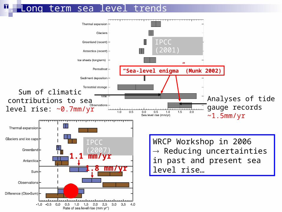
IPCC (2007)

1.1 mm/yr1.8 mm/yr

IPCC (2001)

Sum of climatic contributions to sea level rise: ~0.7mm/yr

“Sea-level enigma” (Munk 2002)

Analyses of tide gauge records ~1.5mm/yr

I. Long term sea level trends

WRCP Workshop in 2006 Reducing uncertainties in past and present sea level rise…

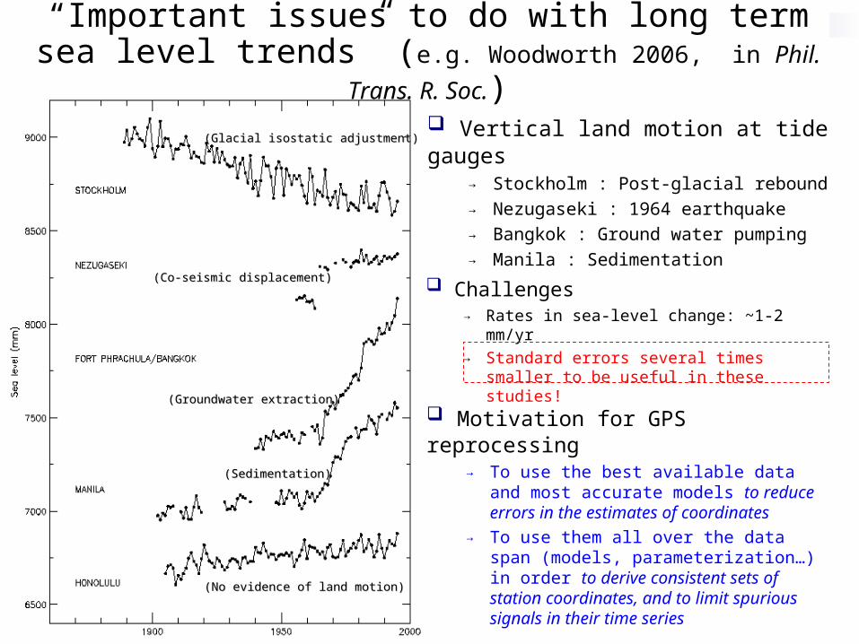
Vertical land motion at tide gauges→ Stockholm : Post-glacial rebound→ Nezugaseki : 1964 earthquake→ Bangkok : Ground water pumping→ Manila : Sedimentation

“Important issues to do with long term sea level trends” (e.g. Woodworth 2006, in Phil. Trans. R. Soc.)

Motivation for GPS reprocessing→ To use the best available data and

most accurate models to reduce errors in the estimates of coordinates

→ To use them all over the data span (models, parameterization…) in order to derive consistent sets of station coordinates, and to limit spurious signals in their time series

Challenges→ Rates in sea-level change: ~1-2 mm/yr→ Standard errors several times smaller

to be useful in these studies!

(Glacial isostatic adjustment)(Glacial isostatic adjustment)

(Co-seismic displacement)(Co-seismic displacement)

(Groundwater extraction)(Groundwater extraction)

(Sedimentation)(Sedimentation)

(No evidence of land motion)(No evidence of land motion)

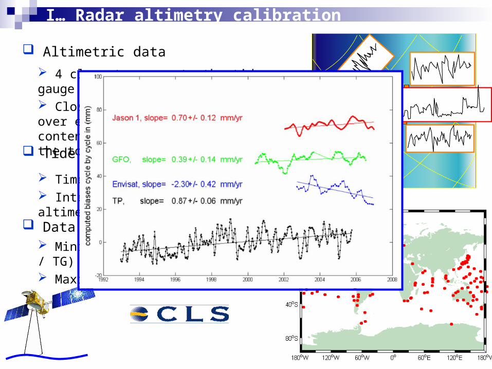
4 closest passes to the tide gauge (Ǿ<160km) Closest points to the tide gauges over each pass, with valid SLA content: 70% of valid values w.r.t. the total # of cycles

Altimetric data

Tide gauge data

Time series > 2 years Interpolation at the epoch of altimetric pass

Data editing (Mitchum 2000)

I… Radar altimetry calibration

Minimum correlation: 0.3 (SLA Alt / TG) Maximum RMS differnces: 100mm

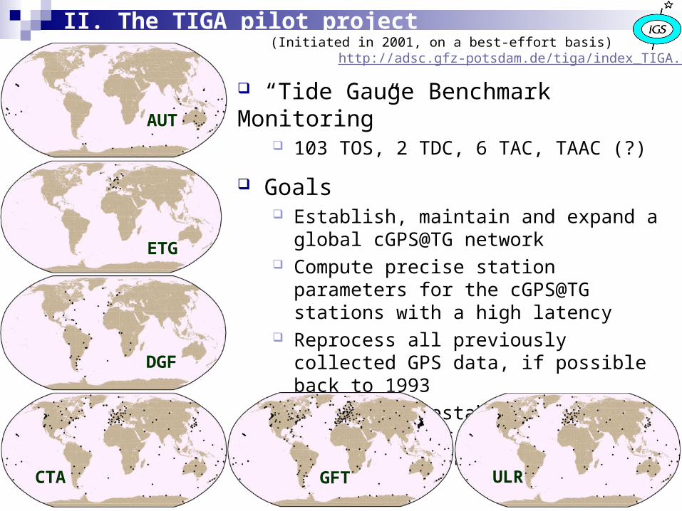
“Tide Gauge Benchmark Monitoring” 103 TOS, 2 TDC, 6 TAC, TAAC (?)

Goals Establish, maintain and expand a global

cGPS@TG network Compute precise station parameters for the

cGPS@TG stations with a high latency Reprocess all previously collected GPS data,

if possible back to 1993 Promote the establishment of links to other

geodetic sites (DORIS, SLR, VLBI,… AG)

(Initiated in 2001, on a best-effort basis)http://adsc.gfz-potsdam.de/tiga/index_TIGA.html

II. The TIGA pilot project

ETG

AUT

DGF

GFTCTA ULR

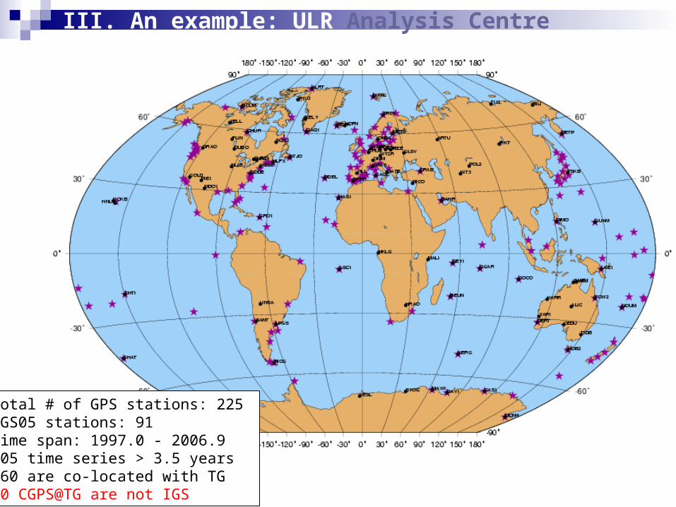
Total # of GPS stations: 225 IGS05 stations: 91 Time span: 1997.0 - 2006.9 205 time series > 3.5 years 160 are co-located with TG 90 CGPS@TG are not IGS

III. An example: ULR Analysis Centre

Parameter Description

GPS Software

Stations Data Sessions and sampling Elevation cut-off angle Ionosphere refraction Troposphere refraction Antenna PCV Earth orientation Earth and polar tide Ocean tide loading Station positions Orbits Reference Frame Combination strategy

GAMIT 10.21 (King and Bock 2006) for GPS observations processing

Grouping into five 50-stations global sub-networks (50-stations at most) Double-differenced phase and code pseudo-range observations 24-hour sessions; 5 min. sampling interval (data cleaning: 30s) 10° Ionosphere-free linear combination LC (1st-order effect eliminated) A priori zenith delays from Saastamoinen (1973) model, using a standard atmosphere, mapped with the GMF mapping functions (Boehm et al. 2006); zenith wet delays estimated as a piece-wise linear model with 2-h nodes, plus gradients in north-south and east-west directions at 24-h intervals. IGS absolute phase centre corrections (Gendt 2005, IGSMAIL-5272) for both the tracking and transmitting antennas IERS bulletin B IERS2003 (Petit and McCarthy 2004). Computed using CSR4.0 ocean tide model and the facility provided by Scherneck and Bos (http://www.oso.chalmers.se/~loading/). Free network approach. A priori values either from ITRF2000 or ITRF2005 (according to the foreseen solution). Position constraints at 1 meter. Adjusted (relaxed orbit strategy). A priori values from IGS precise orbits. Orbit parameter constraints equivalent to ~20 cm. BERNE Radiation model. ITRF2005 datum, 86 out of the 91 IGb05 stations (see Figure 1). GOLD, JAB1, REYK, YAR1, MCM4, excluded due to large residuals. The global GPS sub-network solutions are combined into daily and weekly solutions, and aligned to the ITRF2005 using the minimum constraint approach implemented in the CATREF Software (Altamimi et al. 2004)

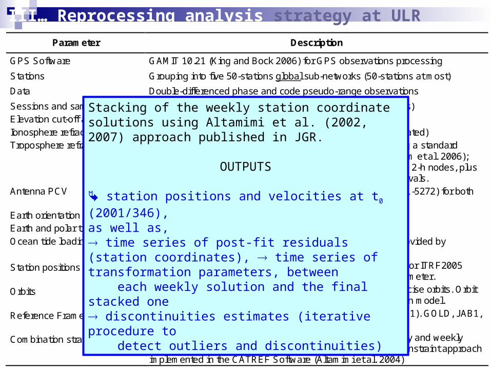
III… Reprocessing analysis strategy at ULR

Stacking of the weekly station coordinate solutions using Altamimi et al. (2002, 2007) approach published in JGR.

OUTPUTS

station positions and velocities at t0 (2001/346), as well as, time series of post-fit residuals (station coordinates), time series of transformation parameters, between each weekly solution and the final stacked one discontinuities estimates (iterative procedure to detect outliers and discontinuities)

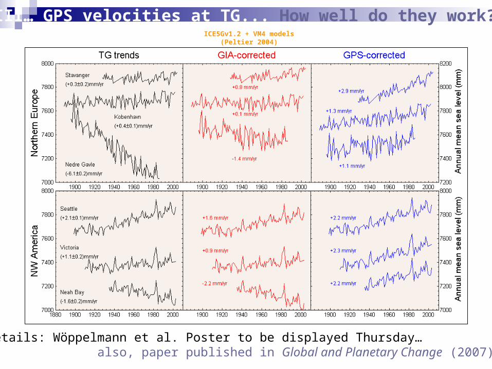
III… GPS velocities at TG... How well do they work?

For details: Wöppelmann et al. Poster to be displayed Thursday… also, paper published in Global and Planetary Change (2007)

ICE5Gv1.2 + VM4 models(Peltier 2004)

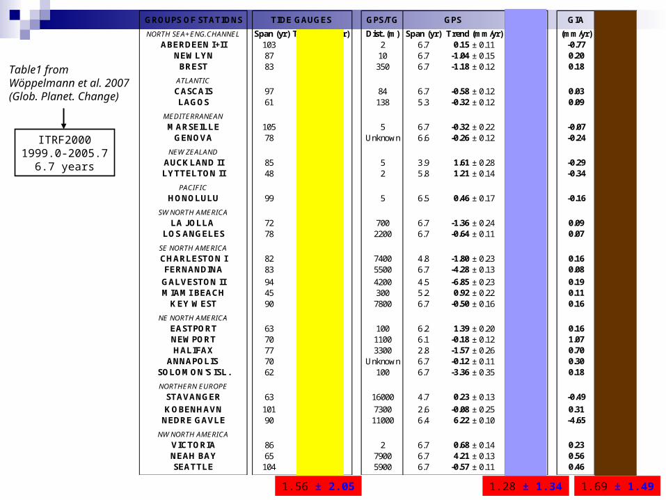
GROUPS OF STATIONS TIDE GAUGES GPS/TG GPS TG+GPS GIA TG-GIA

NORTH SEA+ENG.CHANNEL Span (yr) Trend (mm/yr) Dist. (m) Span (yr) Trend (mm/yr) (mm/yr) (mm/yr) (mm/yr)ABERDEEN I+II 103 0.58 ± 0.10 2 6.7 0.15 ± 0.11 0.73 -0.77 1.35

NEWLYN 87 1.69 ± 0.11 10 6.7 -1.04 ± 0.15 0.65 0.20 1.49BREST 83 1.40 ± 0.05 350 6.7 -1.18 ± 0.12 0.22 0.18 1.22

ATLANTICCASCAIS 97 1.22 ± 0.10 84 6.7 -0.58 ± 0.12 0.64 0.03 1.19LAGOS 61 1.35 ± 0.18 138 5.3 -0.32 ± 0.12 1.03 0.09 1.26

MEDITERRANEANMARSEILLE 105 1.27 ± 0.09 5 6.7 -0.32 ± 0.22 0.95 -0.07 1.34

GENOVA 78 1.20 ± 0.07 Unknown 6.6 -0.26 ± 0.12 0.94 -0.24 1.44

NEW ZEALANDAUCKLAND II 85 1.30 ± 0.13 5 3.9 1.61 ± 0.28 2.91 -0.29 1.59LYTTELTON II 48 2.30 ± 0.21 2 5.8 1.21 ± 0.14 3.51 -0.34 2.64

PACIFICHONOLULU 99 1.46 ± 0.13 5 6.5 0.46 ± 0.17 1.92 -0.16 1.62

SW NORTH AMERICALA JOLLA 72 2.11 ± 0.16 700 6.7 -1.36 ± 0.24 0.75 0.09 2.02

LOS ANGELES 78 0.86 ± 0.15 2200 6.7 -0.64 ± 0.11 0.22 0.07 0.79SE NORTH AMERICACHARLESTON I 82 3.23 ± 0.16 7400 4.8 -1.80 ± 0.23 1.43 0.16 3.06FERNANDINA 83 2.00 ± 0.13 5500 6.7 -4.28 ± 0.13 -2.28 0.08 1.92

GALVESTON II 94 6.47 ± 0.17 4200 4.5 -6.85 ± 0.23 -0.38 0.19 6.28MIAMI BEACH 45 2.29 ± 0.26 300 5.2 0.92 ± 0.22 3.21 0.11 2.18

KEY WEST 90 2.23 ± 0.10 7800 6.7 -0.50 ± 0.16 1.73 0.16 2.07

NE NORTH AMERICAEASTPORT 63 2.07 ± 0.16 100 6.2 1.39 ± 0.20 3.46 0.16 1.91NEWPORT 70 2.48 ± 0.14 1100 6.1 -0.18 ± 0.12 2.3 1.07 1.41HALIFAX 77 3.29 ± 0.11 3300 2.8 -1.57 ± 0.26 1.72 0.70 2.59

ANNAPOLIS 70 3.46 ± 0.17 Unknown 6.7 -0.12 ± 0.11 3.34 0.30 3.16SOLOMON'S ISL. 62 3.36 ± 0.19 100 6.7 -3.36 ± 0.35 0.00 0.18 3.18NORTHERN EUROPE

STAVANGER 63 0.27 ± 0.17 16000 4.7 0.23 ± 0.13 0.50 -0.49 0.76KOBENHAVN 101 0.32 ± 0.12 7300 2.6 -0.08 ± 0.25 0.24 0.31 0.01

NEDRE GAVLE 90 -6.05 ± 0.23 11000 6.4 6.22 ± 0.10 0.17 -4.65 -1.40

NW NORTH AMERICAVICTORIA 86 1.10 ± 0.15 2 6.7 0.68 ± 0.14 1.78 0.23 0.87NEAH BAY 65 -1.59 ± 0.22 7900 6.7 4.21 ± 0.13 2.62 0.56 -2.15SEATTLE 104 2.06 ± 0.11 5900 6.7 -0.57 ± 0.11 1.49 0.46 1.60

Table1 fromWöppelmann et al. 2007(Glob. Planet. Change)

1.28 ± 1.34 1.69 ± 1.491.56 ± 2.05

ITRF20001999.0-2005.7

6.7 years

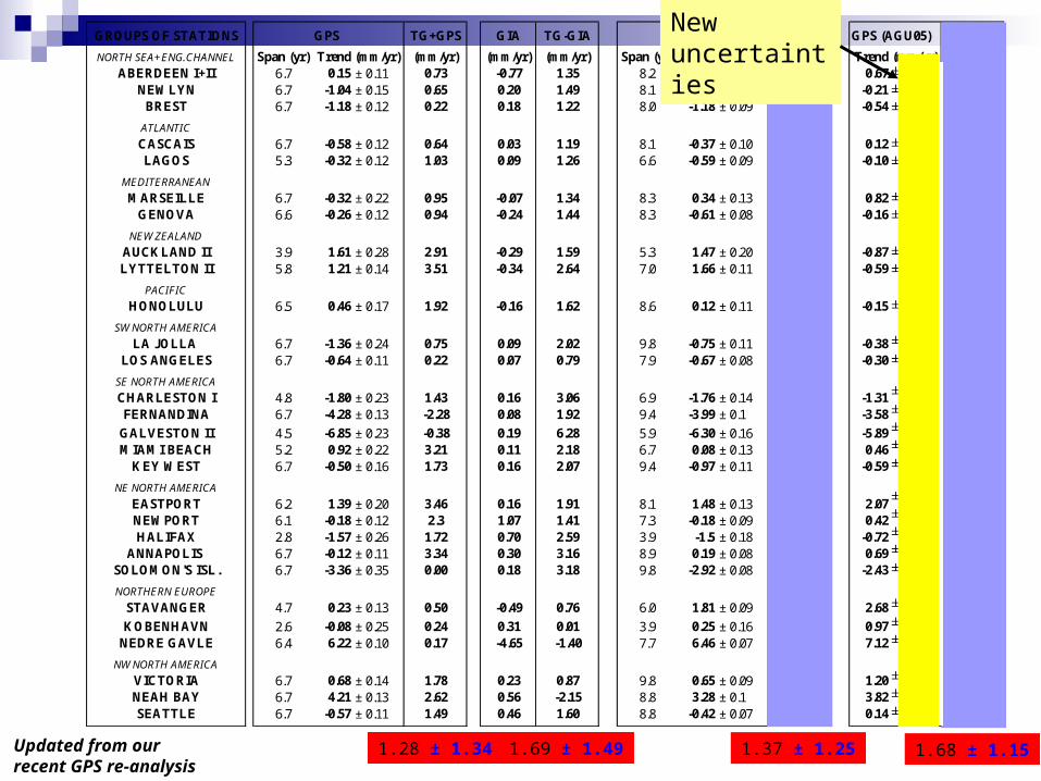
GROUPS OF STATIONS GPS TG+GPS GIA TG-GIA GPS (AGU00) TG+GPS GPS (AGU05) TG+GPSNORTH SEA+ENG.CHANNEL Span (yr) Trend (mm/yr) (mm/yr) (mm/yr) (mm/yr) Span (yr) Trend (mm/yr) (mm/yr) Trend (mm/yr) (mm/yr)

ABERDEEN I+II 6.7 0.15 ± 0.11 0.73 -0.77 1.35 8.2 -0.10 ± 0.10 0.48 0.67 ± 0.04 1.25NEWLYN 6.7 -1.04 ± 0.15 0.65 0.20 1.49 8.1 -0.90 ± 0.08 0.79 -0.21 ± 0.03 1.48

BREST 6.7 -1.18 ± 0.12 0.22 0.18 1.22 8.0 -1.18 ± 0.09 0.22 -0.54 ± 0.04 0.86ATLANTICCASCAIS 6.7 -0.58 ± 0.12 0.64 0.03 1.19 8.1 -0.37 ± 0.10 0.85 0.12 ± 0.04 1.34LAGOS 5.3 -0.32 ± 0.12 1.03 0.09 1.26 6.6 -0.59 ± 0.09 0.76 -0.10 ± 0.04 1.25

MEDITERRANEANMARSEILLE 6.7 -0.32 ± 0.22 0.95 -0.07 1.34 8.3 0.34 ± 0.13 1.61 0.82 ± 0.05 2.09

GENOVA 6.6 -0.26 ± 0.12 0.94 -0.24 1.44 8.3 -0.61 ± 0.08 0.59 -0.16 ± 0.04 1.04NEW ZEALAND

AUCKLAND II 3.9 1.61 ± 0.28 2.91 -0.29 1.59 5.3 1.47 ± 0.20 2.77 -0.87 ± 0.08 0.43LYTTELTON II 5.8 1.21 ± 0.14 3.51 -0.34 2.64 7.0 1.66 ± 0.11 3.96 -0.59 ± 0.05 1.71

PACIFICHONOLULU 6.5 0.46 ± 0.17 1.92 -0.16 1.62 8.6 0.12 ± 0.11 1.58 -0.15 ± 0.05 1.31

SW NORTH AMERICALA JOLLA 6.7 -1.36 ± 0.24 0.75 0.09 2.02 9.8 -0.75 ± 0.11 1.36 -0.38 ± 0.05 1.73

LOS ANGELES 6.7 -0.64 ± 0.11 0.22 0.07 0.79 7.9 -0.67 ± 0.08 0.19 -0.30 ± 0.04 0.56SE NORTH AMERICACHARLESTON I 4.8 -1.80 ± 0.23 1.43 0.16 3.06 6.9 -1.76 ± 0.14 1.47 -1.31 ± 0.06 1.92FERNANDINA 6.7 -4.28 ± 0.13 -2.28 0.08 1.92 9.4 -3.99 ± 0.1 -1.99 -3.58 ± 0.04 -1.58

GALVESTON II 4.5 -6.85 ± 0.23 -0.38 0.19 6.28 5.9 -6.30 ± 0.16 0.17 -5.89 ± 0.07 0.58MIAMI BEACH 5.2 0.92 ± 0.22 3.21 0.11 2.18 6.7 0.08 ± 0.13 2.37 0.46 ± 0.06 2.75

KEY WEST 6.7 -0.50 ± 0.16 1.73 0.16 2.07 9.4 -0.97 ± 0.11 1.26 -0.59 ± 0.05 1.64NE NORTH AMERICA

EASTPORT 6.2 1.39 ± 0.20 3.46 0.16 1.91 8.1 1.48 ± 0.13 3.55 2.07 ± 0.06 4.14NEWPORT 6.1 -0.18 ± 0.12 2.3 1.07 1.41 7.3 -0.18 ± 0.09 2.3 0.42 ± 0.04 2.9HALIFAX 2.8 -1.57 ± 0.26 1.72 0.70 2.59 3.9 -1.5 ± 0.18 1.79 -0.72 ± 0.07 2.57

ANNAPOLIS 6.7 -0.12 ± 0.11 3.34 0.30 3.16 8.9 0.19 ± 0.08 3.65 0.69 ± 0.04 4.15SOLOMON'S ISL. 6.7 -3.36 ± 0.35 0.00 0.18 3.18 9.8 -2.92 ± 0.08 0.44 -2.43 ± 0.03 0.93NORTHERN EUROPE

STAVANGER 4.7 0.23 ± 0.13 0.50 -0.49 0.76 6.0 1.81 ± 0.09 2.08 2.68 ± 0.04 2.95KOBENHAVN 2.6 -0.08 ± 0.25 0.24 0.31 0.01 3.9 0.25 ± 0.16 0.57 0.97 ± 0.06 1.29

NEDRE GAVLE 6.4 6.22 ± 0.10 0.17 -4.65 -1.40 7.7 6.46 ± 0.07 0.41 7.12 ± 0.03 1.07NW NORTH AMERICA

VICTORIA 6.7 0.68 ± 0.14 1.78 0.23 0.87 9.8 0.65 ± 0.09 1.75 1.20 ± 0.04 2.30NEAH BAY 6.7 4.21 ± 0.13 2.62 0.56 -2.15 8.8 3.28 ± 0.1 1.69 3.82 ± 0.04 2.23SEATTLE 6.7 -0.57 ± 0.11 1.49 0.46 1.60 8.8 -0.42 ± 0.07 1.64 0.14 ± 0.03 2.20

Updated from ourrecent GPS re-analysis

1.28 ± 1.34 1.69 ± 1.49 1.37 ± 1.25 1.68 ± 1.15

Newuncertainties

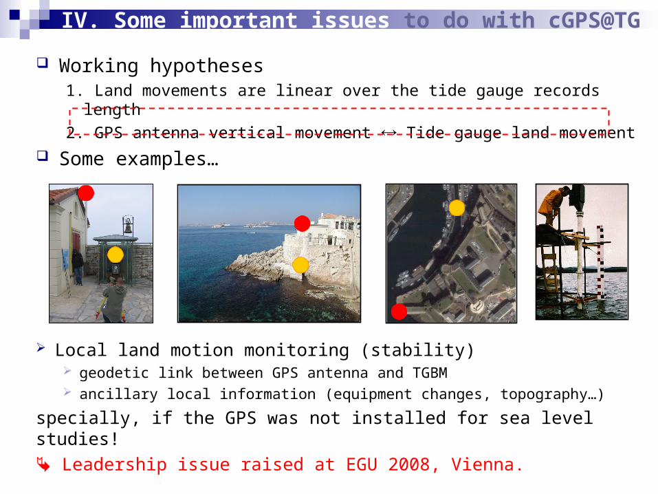
Working hypotheses1. Land movements are linear over the tide gauge records length2. GPS antenna vertical movement Tide gauge land movement

Some examples…

IV. Some important issues to do with cGPS@TG

Local land motion monitoring (stability) geodetic link between GPS antenna and TGBM ancillary local information (equipment changes, topography…)

specially, if the GPS was not installed for sea level studies! Leadership issue raised at EGU 2008, Vienna.

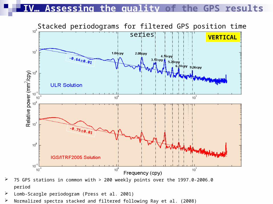
IV… Assessing the quality of the GPS results

VERTICAL

-0.750.01

-0.640.01

75 GPS stations in common with > 200 weekly points over the 1997.0-2006.0 period Lomb-Scargle periodogram (Press et al. 2001) Normalized spectra stacked and filtered following Ray et al. (2008) approach

(annual and semi-annual fits have been removed prior to spectra computation)

Stacked periodograms for filtered GPS position time series

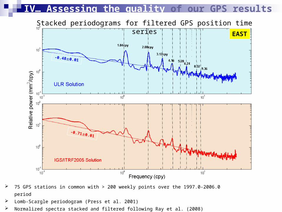
-0.480.01

-0.710.01

EASTStacked periodograms for filtered GPS position time series

IV… Assessing the quality of our GPS results

75 GPS stations in common with > 200 weekly points over the 1997.0-2006.0 period Lomb-Scargle periodogram (Press et al. 2001) Normalized spectra stacked and filtered following Ray et al. (2008) approach

(annual and semi-annual fits have been removed prior to spectra computation)

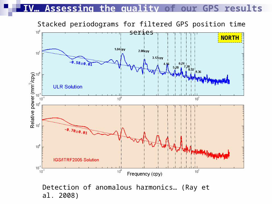
NORTH

-0.580.01

-0.700.01

Stacked periodograms for filtered GPS position time series

IV… Assessing the quality of our GPS results

Detection of anomalous harmonics… (Ray et al. 2008)

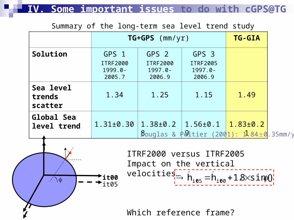
ITRF2000 versus ITRF2005Impact on the vertical velocities…

Which reference frame?

IV. Some important issues to do with cGPS@TG

TG+GPS (mm/yr) TG-GIA

Solution GPS 1ITRF2000

1999.0-2005.7

GPS 2 ITRF2000

1997.0-2006.9

GPS 3ITRF2005

1997.0-2006.9

Sea level trends scatter 1.34 1.25 1.15 1.49

Global Sea level trend 1.31±0.30 1.38±0.28 1.56±0.19 1.83±0.21

Summary of the long-term sea level trend study

Douglas & Peltier (2001): 1.840.35mm/yr

it05it00 )sin(8.1hh 00it05it

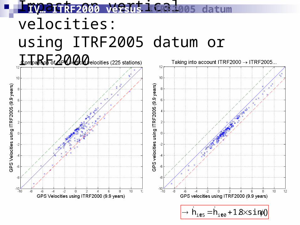
Impact on vertical velocities: using ITRF2005 datum or ITRF2000

)sin(8.1hh 00it05it

IV… ITRF2000 versus ITRF2005 datum

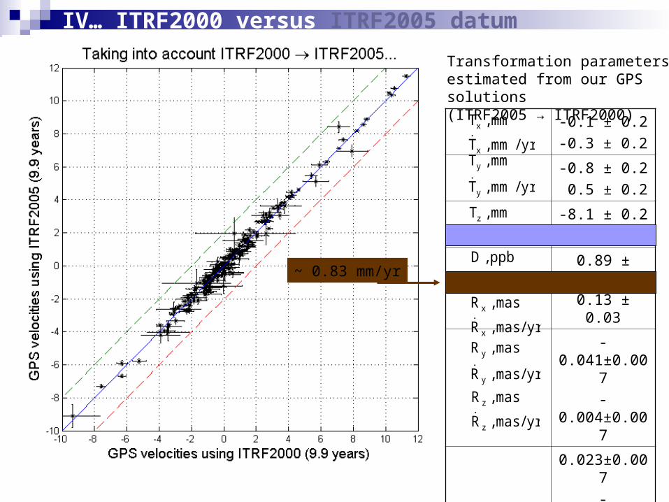
-0.1 ± 0.2-0.3 ± 0.2

-0.8 ± 0.2 0.5 ± 0.2

-8.1 ± 0.2-1.7 ± 0.2

0.89 ± 0.030.13 ± 0.03

-0.041±0.007-0.004±0.007

0.023±0.007-0.003±0.007

-0.052±0.008-0.010±0.008

yr/mm,T

mm,T

x

x

yr/mm,T

mm,T

y

y

yr/mm,T

mm,T

z

z

yr/ppb,D

ppb,D

yr/mas,R

mas,R

x

x

yr/mas,R

mas,R

y

y

yr/mas,R

mas,R

z

z

Transformation parametersestimated from our GPS solutions (ITRF2005 → ITRF2000)

~ 0.83 mm/yr

IV… ITRF2000 versus ITRF2005 datum

GROUPS OF STATIONS GPS TG+GPS GIA TG-GIA GPS (AGU00) TG+GPS GPS (AGU05) TG+GPSNORTH SEA+ENG.CHANNEL Span (yr) Trend (mm/yr) (mm/yr) (mm/yr) (mm/yr) Span (yr) Trend (mm/yr) (mm/yr) Trend (mm/yr) (mm/yr)

ABERDEEN I+II 6.7 0.15 ± 0.11 0.73 -0.77 1.35 8.2 -0.10 ± 0.10 0.48 0.67 ± 0.04 1.25NEWLYN 6.7 -1.04 ± 0.15 0.65 0.20 1.49 8.1 -0.90 ± 0.08 0.79 -0.21 ± 0.03 1.48

BREST 6.7 -1.18 ± 0.12 0.22 0.18 1.22 8.0 -1.18 ± 0.09 0.22 -0.54 ± 0.04 0.86ATLANTICCASCAIS 6.7 -0.58 ± 0.12 0.64 0.03 1.19 8.1 -0.37 ± 0.10 0.85 0.12 ± 0.04 1.34LAGOS 5.3 -0.32 ± 0.12 1.03 0.09 1.26 6.6 -0.59 ± 0.09 0.76 -0.10 ± 0.04 1.25

MEDITERRANEANMARSEILLE 6.7 -0.32 ± 0.22 0.95 -0.07 1.34 8.3 0.34 ± 0.13 1.61 0.82 ± 0.05 2.09

GENOVA 6.6 -0.26 ± 0.12 0.94 -0.24 1.44 8.3 -0.61 ± 0.08 0.59 -0.16 ± 0.04 1.04NEW ZEALAND

AUCKLAND II 3.9 1.61 ± 0.28 2.91 -0.29 1.59 5.3 1.47 ± 0.20 2.77 -0.87 ± 0.08 0.43LYTTELTON II 5.8 1.21 ± 0.14 3.51 -0.34 2.64 7.0 1.66 ± 0.11 3.96 -0.59 ± 0.05 1.71

PACIFICHONOLULU 6.5 0.46 ± 0.17 1.92 -0.16 1.62 8.6 0.12 ± 0.11 1.58 -0.15 ± 0.05 1.31

SW NORTH AMERICALA JOLLA 6.7 -1.36 ± 0.24 0.75 0.09 2.02 9.8 -0.75 ± 0.11 1.36 -0.38 ± 0.05 1.73

LOS ANGELES 6.7 -0.64 ± 0.11 0.22 0.07 0.79 7.9 -0.67 ± 0.08 0.19 -0.30 ± 0.04 0.56SE NORTH AMERICACHARLESTON I 4.8 -1.80 ± 0.23 1.43 0.16 3.06 6.9 -1.76 ± 0.14 1.47 -1.31 ± 0.06 1.92FERNANDINA 6.7 -4.28 ± 0.13 -2.28 0.08 1.92 9.4 -3.99 ± 0.1 -1.99 -3.58 ± 0.04 -1.58

GALVESTON II 4.5 -6.85 ± 0.23 -0.38 0.19 6.28 5.9 -6.30 ± 0.16 0.17 -5.89 ± 0.07 0.58MIAMI BEACH 5.2 0.92 ± 0.22 3.21 0.11 2.18 6.7 0.08 ± 0.13 2.37 0.46 ± 0.06 2.75

KEY WEST 6.7 -0.50 ± 0.16 1.73 0.16 2.07 9.4 -0.97 ± 0.11 1.26 -0.59 ± 0.05 1.64NE NORTH AMERICA

EASTPORT 6.2 1.39 ± 0.20 3.46 0.16 1.91 8.1 1.48 ± 0.13 3.55 2.07 ± 0.06 4.14NEWPORT 6.1 -0.18 ± 0.12 2.3 1.07 1.41 7.3 -0.18 ± 0.09 2.3 0.42 ± 0.04 2.9HALIFAX 2.8 -1.57 ± 0.26 1.72 0.70 2.59 3.9 -1.5 ± 0.18 1.79 -0.72 ± 0.07 2.57

ANNAPOLIS 6.7 -0.12 ± 0.11 3.34 0.30 3.16 8.9 0.19 ± 0.08 3.65 0.69 ± 0.04 4.15SOLOMON'S ISL. 6.7 -3.36 ± 0.35 0.00 0.18 3.18 9.8 -2.92 ± 0.08 0.44 -2.43 ± 0.03 0.93NORTHERN EUROPE

STAVANGER 4.7 0.23 ± 0.13 0.50 -0.49 0.76 6.0 1.81 ± 0.09 2.08 2.68 ± 0.04 2.95KOBENHAVN 2.6 -0.08 ± 0.25 0.24 0.31 0.01 3.9 0.25 ± 0.16 0.57 0.97 ± 0.06 1.29

NEDRE GAVLE 6.4 6.22 ± 0.10 0.17 -4.65 -1.40 7.7 6.46 ± 0.07 0.41 7.12 ± 0.03 1.07NW NORTH AMERICA

VICTORIA 6.7 0.68 ± 0.14 1.78 0.23 0.87 9.8 0.65 ± 0.09 1.75 1.20 ± 0.04 2.30NEAH BAY 6.7 4.21 ± 0.13 2.62 0.56 -2.15 8.8 3.28 ± 0.1 1.69 3.82 ± 0.04 2.23SEATTLE 6.7 -0.57 ± 0.11 1.49 0.46 1.60 8.8 -0.42 ± 0.07 1.64 0.14 ± 0.03 2.20

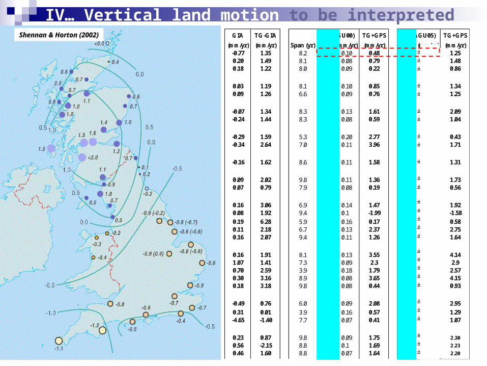
IV… Vertical land motion to be interpretedInferred from PSMSL (2005)Inferred from PSMSL (2005)and Holgate & Woodworth (2004)and Holgate & Woodworth (2004)

Shennan & Horton (2002)Shennan & Horton (2002)

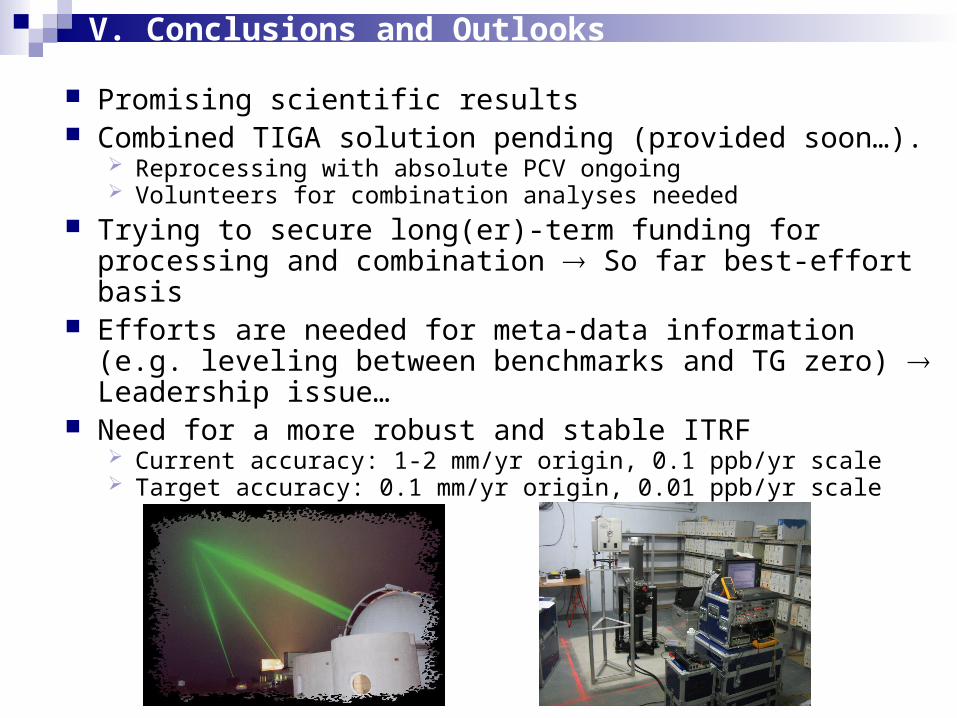
Promising scientific results Combined TIGA solution pending (provided soon…).

Reprocessing with absolute PCV ongoing Volunteers for combination analyses needed

Trying to secure long(er)-term funding for processing and combination So far best-effort basis

Efforts are needed for meta-data information (e.g. leveling between benchmarks and TG zero) Leadership issue…

Need for a more robust and stable ITRF Current accuracy: 1-2 mm/yr origin, 0.1 ppb/yr scale Target accuracy: 0.1 mm/yr origin, 0.01 ppb/yr scale

V. Conclusions and Outlooks

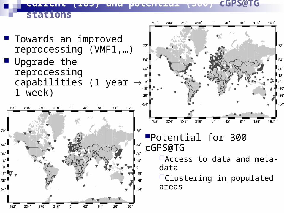
Current (103) and potential (300) cGPS@TG stations

Towards an improved reprocessing (VMF1,…)

Upgrade the reprocessing capabilities (1 year 1 week)

Potential for 300 cGPS@TGAccess to data and meta-dataClustering in populated areas

Thank you for your attention !

View of La Rochelle

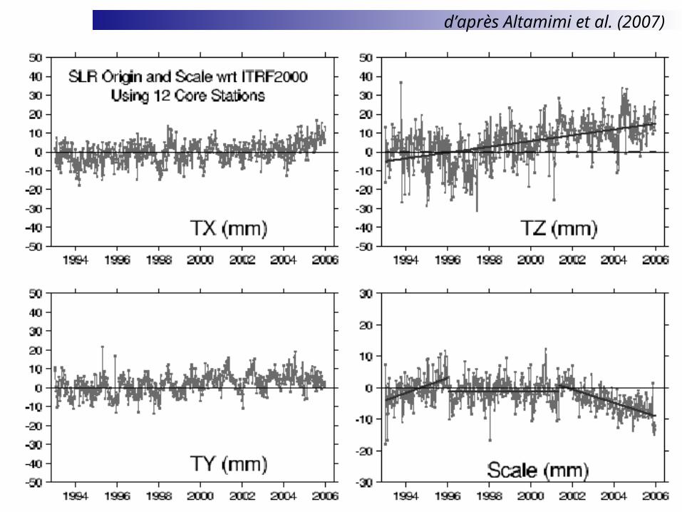
d’après Altamimi et al. (2007)

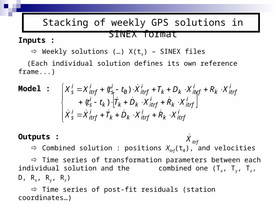
Inputs : Weekly solutions (…) X(ts) – SINEX files

(Each individual solution defines its own reference frame...)

Model :

Outputs : Combined solution : positions Xitrf(t0), and velocities

Time series of transformation parameters between each individual solution and the combined one (Tx, Ty, Tz, D, Rx, Ry, Rz)

Time series of post-fit residuals (station coordinates…)

The reference frame is defined by applying minimal constraintsModel implemented in CATREF (Altamimi, 2004)

Stacking of weekly GPS solutions in SINEX format

iitrfk

iitrfkk

iitrf

is

iitrfk

iitrfkkk

is

iitrfk

iitrfkk

iitrf

is

iitrf

is

XRXDTXXXRXDTtt

XRXDTXttXX

)()( 0

itrfX

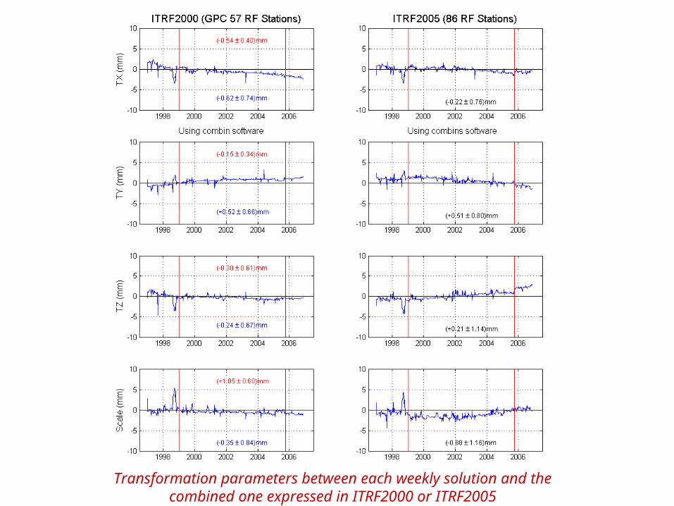
Transformation parameters between each weekly solution and the combined one expressed in ITRF2000 or ITRF2005

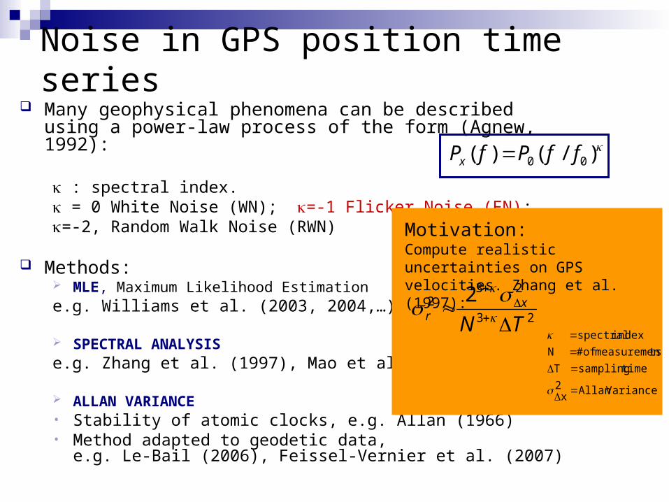
Many geophysical phenomena can be described using a power-law process of the form (Agnew, 1992):

: spectral index. = 0 White Noise (WN); =-1 Flicker Noise (FN); =-2, Random Walk Noise (RWN)

Methods: MLE, Maximum Likelihood Estimatione.g. Williams et al. (2003, 2004,…)

SPECTRAL ANALYSISe.g. Zhang et al. (1997), Mao et al. (1999)

ALLAN VARIANCE• Stability of atomic clocks, e.g. Allan (1966)• Method adapted to geodetic data,

e.g. Le-Bail (2006), Feissel-Vernier et al. (2007)

Noise in GPS position time series

)/()( 00 ffPfPx

23

232 2

TNx

r

VarianceAllan2x

timesamplingTtsmeasuremenof#N

indexspectral

Motivation:Compute realistic uncertainties on GPS velocities. Zhang et al. (1997):

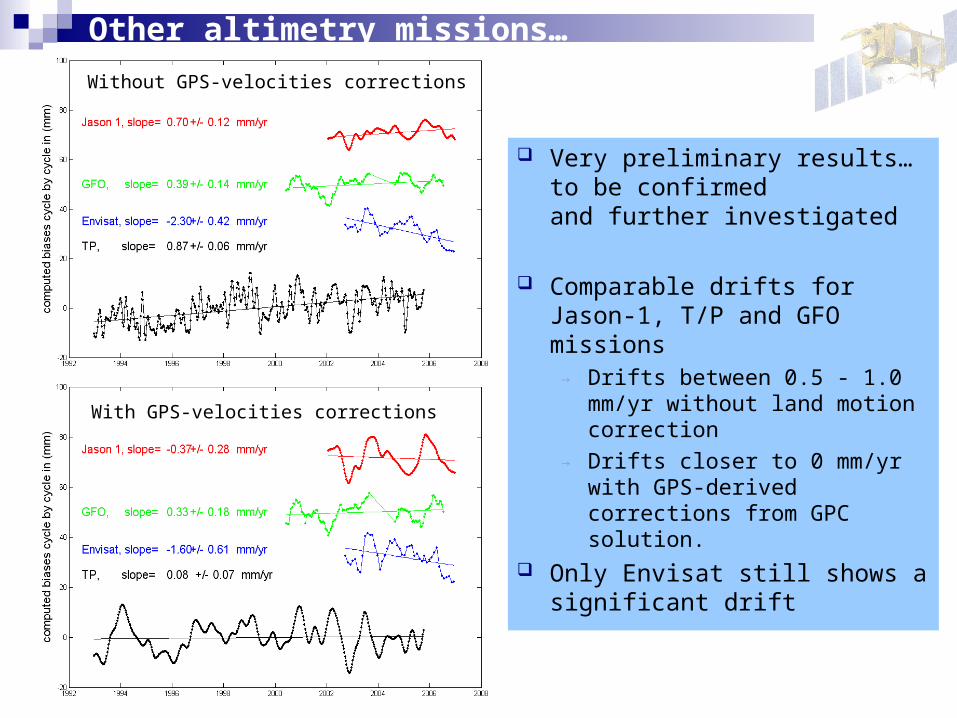
Very preliminary results… to be confirmed and further investigated

Comparable drifts for Jason-1, T/P and GFO missions

→ Drifts between 0.5 - 1.0 mm/yr without land motion correction

→ Drifts closer to 0 mm/yr with GPS-derived corrections from GPC solution.

Only Envisat still shows a significant drift

Other altimetry missions…Without GPS-velocities corrections

With GPS-velocities corrections