Replacement of mining trucks
Víctor Barrientos Boccardo
Jefe Mantenimiento Mina
Cerro Negro Norte I CAP Minería
INDEX
1. Introduction
2. Developed methodology
3. Results3. Results
4. Conclusions & limitations
1/30
1. Introduction
2. Developed methodology
3. Results
INDEX
3. Results
4. Conclusions & limitations
2/30
1. Introduction
In this study, we address the issues of
replacement of mining truck with
60.000 operating hours
3/30
1. Introduction
In this study, we want to determine for
mining trucks 60,000 hours of operation (8
years) which would have been the time of
replacement and if now is the time to do itreplacement and if now is the time to do it
4/30
1. Introduction
a) We have reliable information
maintenance costs and useful lives
major and minor components
b) These trucks are used in an open pit
mine
5/30
1. Introduction
c) Downtime costs or costs not produce are
included for this study
d) The maintenance outsourcing (dealer)
6/30
1. Introduction
2. Developed methodology
3. Results
INDEX
3. Results
4. Conclusions & limitations
7/30
It uses the methodology of calculation of
equivalent annual costs (EAC) to
determine which year should have
replaced mining trucksreplaced mining trucks
8/30
2. Equivale
equivalent annual costs (EAC) nt
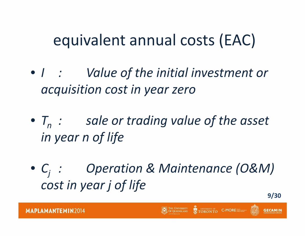
Annual Costs• I : Value of the initial investment or
acquisition cost in year zero
• T : sale or trading value of the asset• Tn : sale or trading value of the asset
in year n of life
• Cj : Operation & Maintenance (O&M)
cost in year j of life9/30
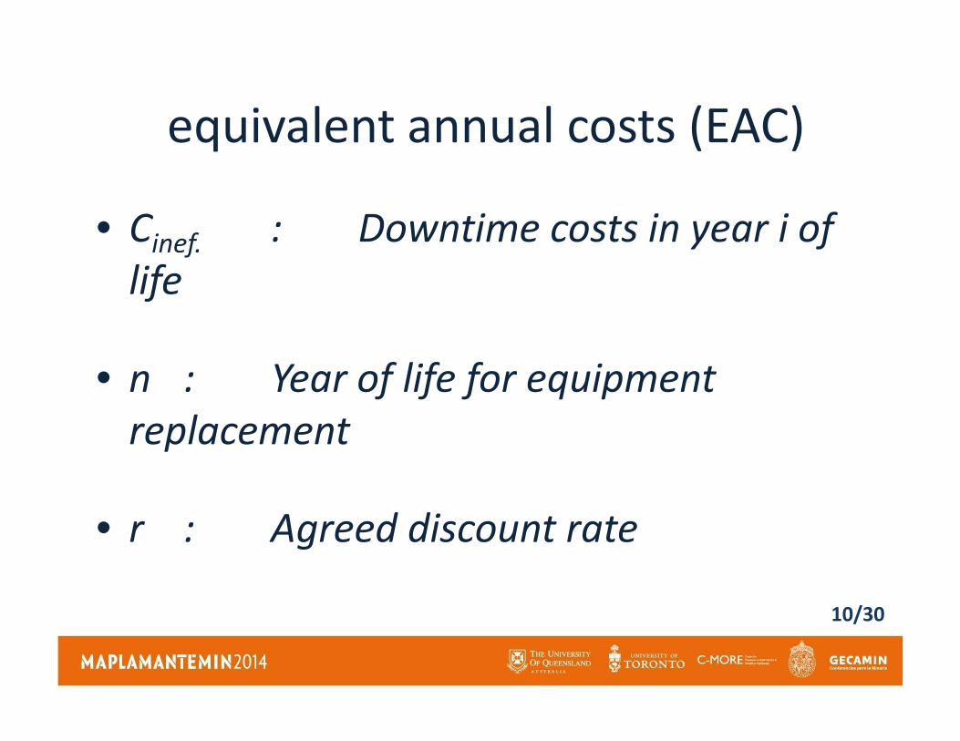
• Cinef. : Downtime costs in year i of
life
• n : Year of life for equipment
2. Equivale
equivalent annual costs (EAC) nt
Annual Costs
• n : Year of life for equipment
replacement
• r : Agreed discount rate
10/30
How the methodology of
Equivalente Annual Cost (EAC)
is mathematically expresed?
11/30
is mathematically expresed?
2. Methodology
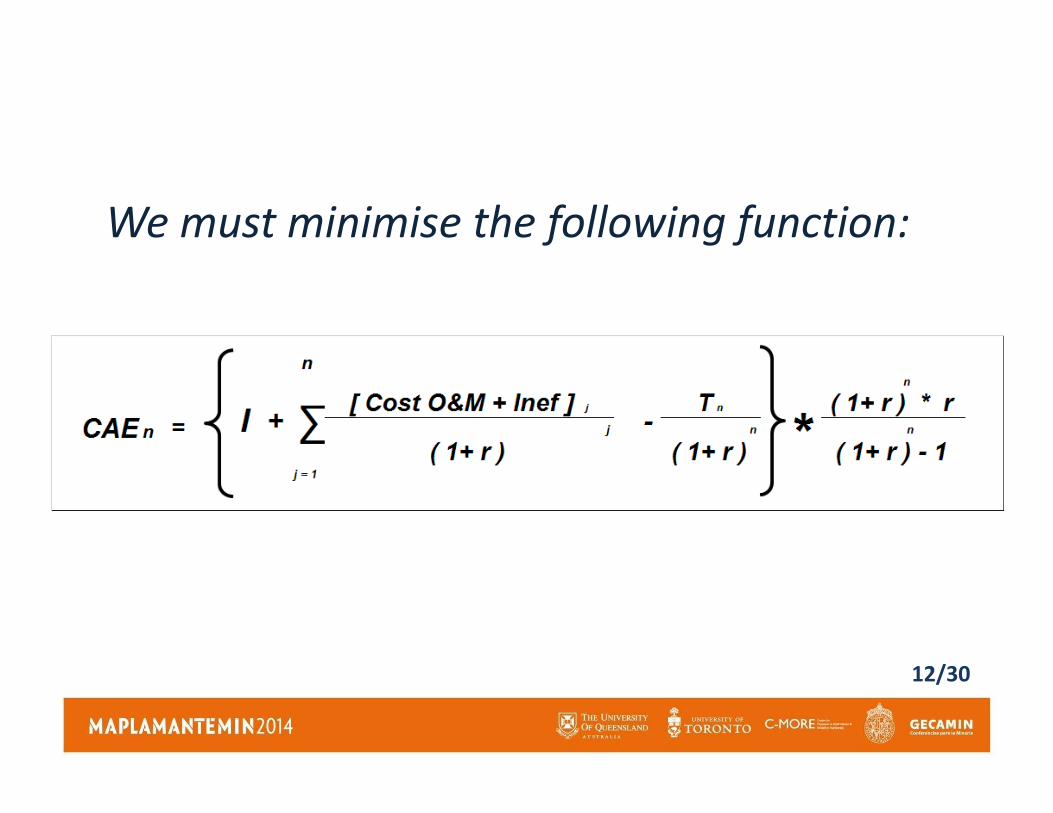
We must minimise the following function:
12/30

We make a sensitivity analysis for the sale
of the Asset Sale of ten form of
depreciation
13/30
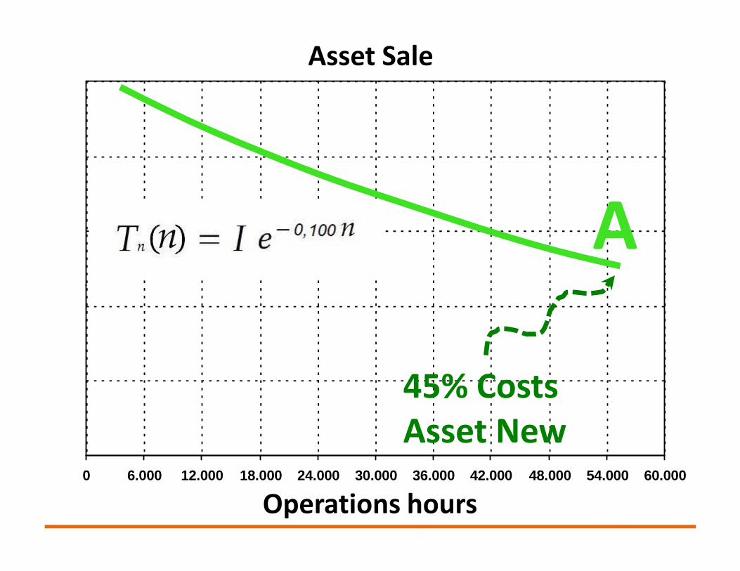
Asset Sale
A
0 6.000 12.000 18.000 24.000 30.000 36.000 42.000 48.000 54.000 60.000
Operations hours
45% Costs
Asset New
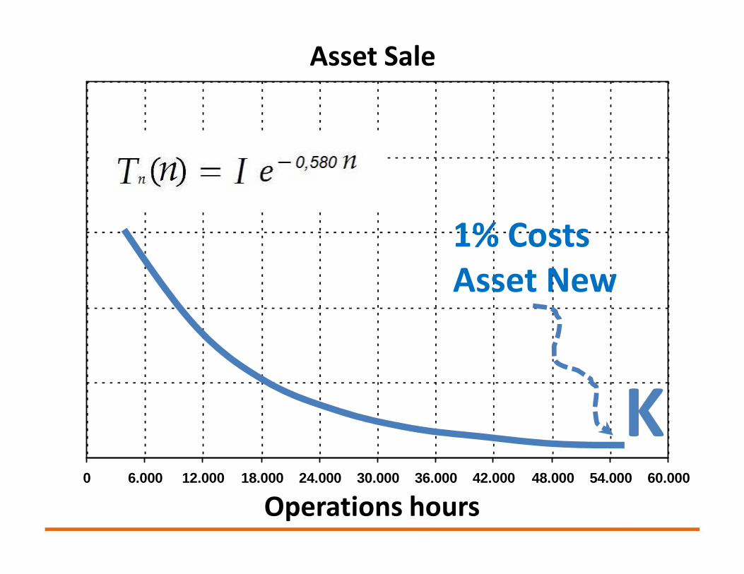
Asset Sale
1% Costs
Asset New
0 6.000 12.000 18.000 24.000 30.000 36.000 42.000 48.000 54.000 60.000
Operations hours
Asset New
K
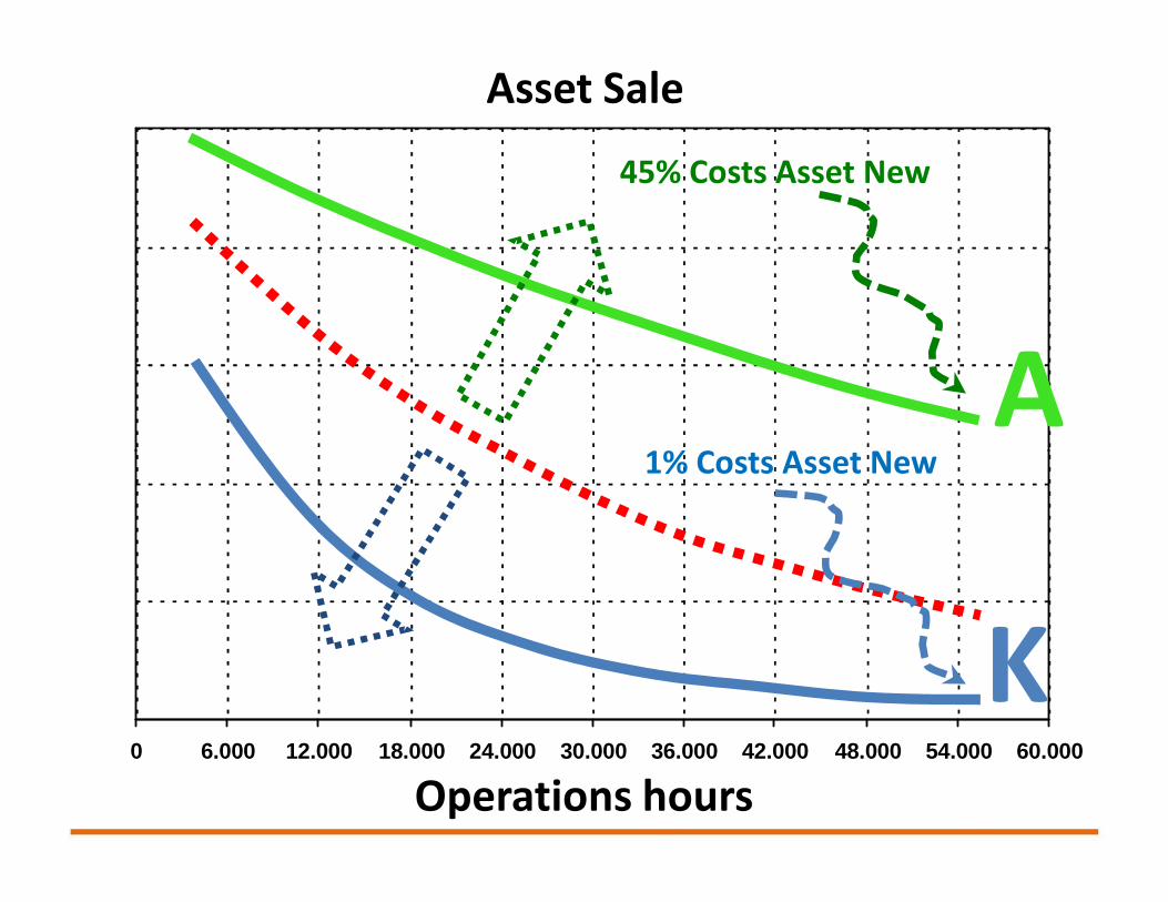
Asset Sale
45% Costs Asset New
1% Costs Asset New
A
0 6.000 12.000 18.000 24.000 30.000 36.000 42.000 48.000 54.000 60.000
Operations hours
1% Costs Asset New
K
A
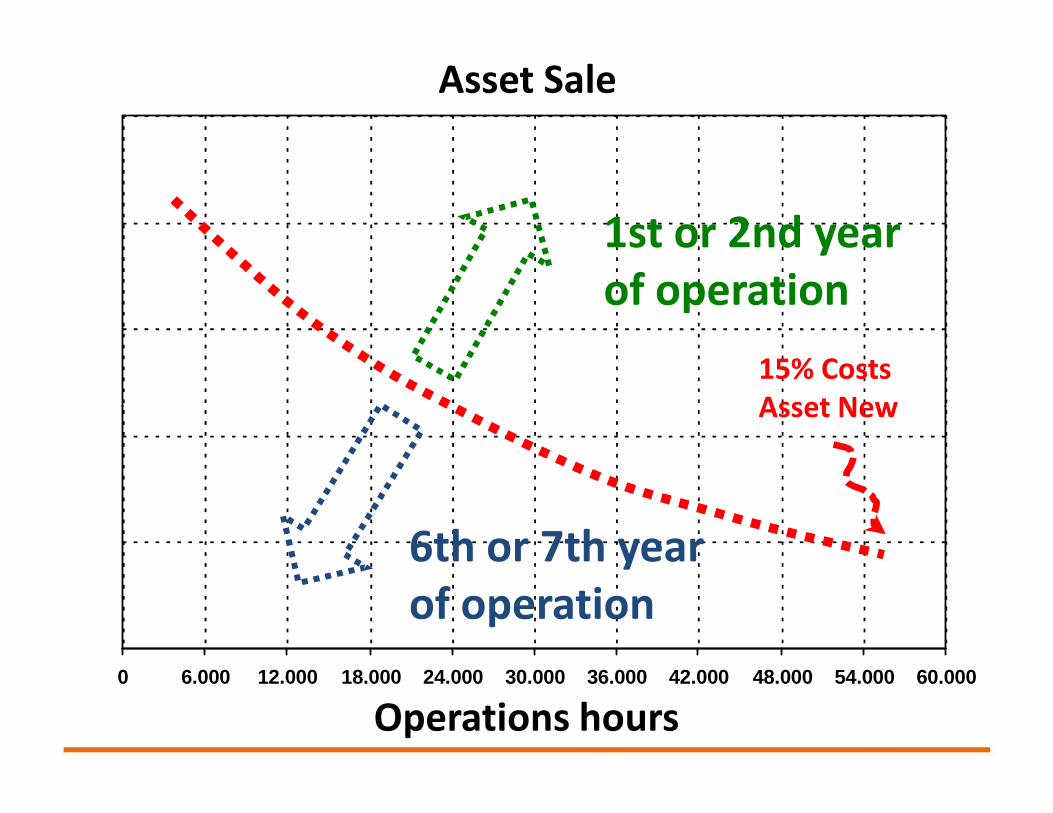
Asset Sale
1st or 2nd year
of operation
15% Costs
Asset New
0 6.000 12.000 18.000 24.000 30.000 36.000 42.000 48.000 54.000 60.000
Operations hours
6th or 7th year
of operation
Asset New
1. Introduction
2. Developed methodology
3. Results
INDEX
3. Results
4. Conclusions & limitations
18/30
3. Results
In a 2-dimensional graph
considering
X-axis: Hour meter of the equipmentX-axis: Hour meter of the equipment
(hours)
Y-axis: Dollars (US$)
19/30
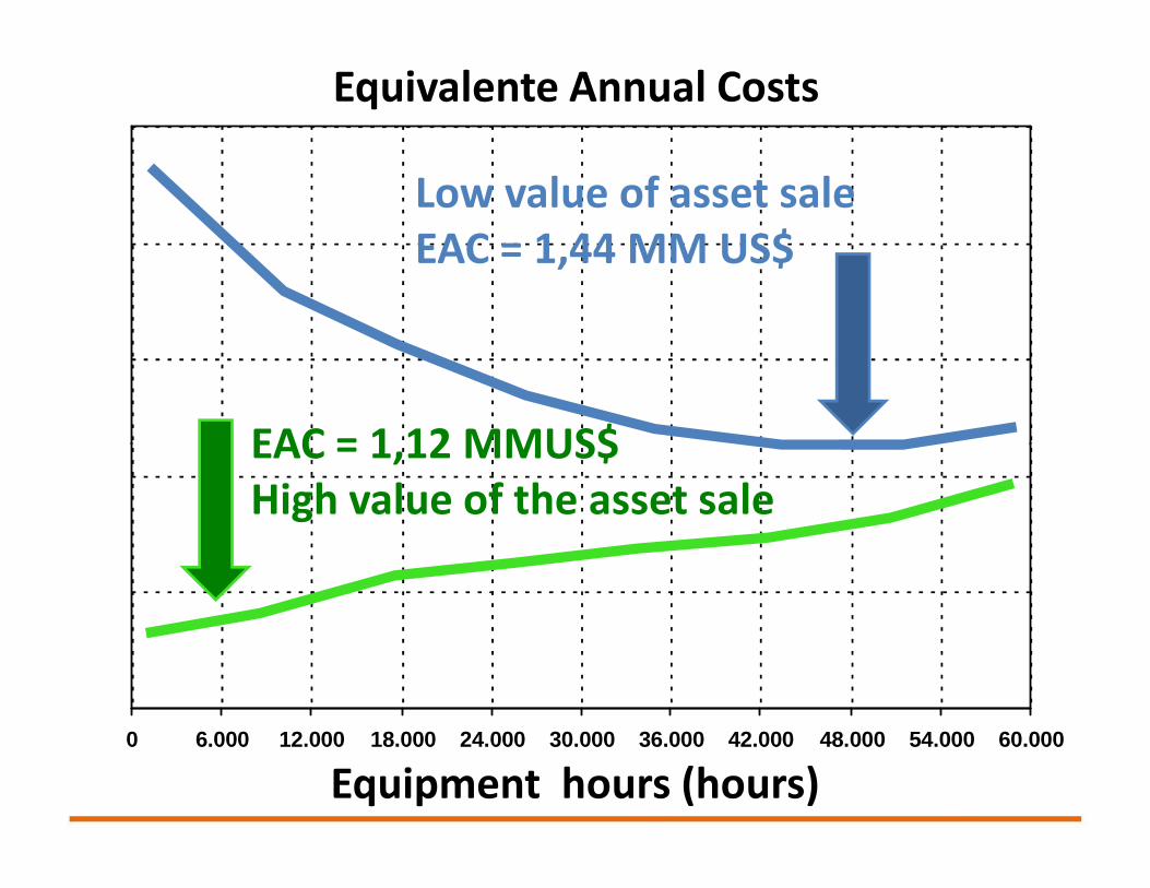
Equivalente Annual Costs
EAC = 1,12 MMUS$
Low value of asset sale
EAC = 1,44 MM US$
0 6.000 12.000 18.000 24.000 30.000 36.000 42.000 48.000 54.000 60.000
Equipment hours (hours)
EAC = 1,12 MMUS$
High value of the asset sale
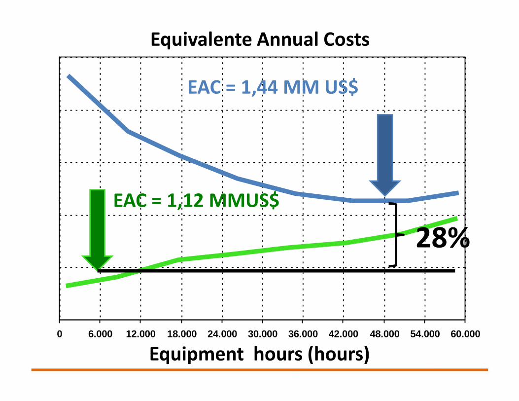
Equivalente Annual Costs
EAC = 1,12 MMUS$
EAC = 1,44 MM US$
0 6.000 12.000 18.000 24.000 30.000 36.000 42.000 48.000 54.000 60.000
Equipment hours (hours)
EAC = 1,12 MMUS$
28%
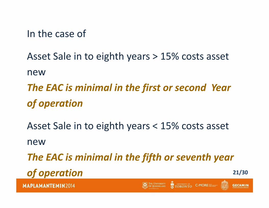
In the case of
Asset Sale in to eighth years > 15% costs asset
new
The EAC is minimal in the first or second Year
of operationof operation
Asset Sale in to eighth years < 15% costs asset
new
The EAC is minimal in the fifth or seventh year
of operation 21/30
1. Introductions
2. Developed methodology
3. Results
INDEX
3. Results
4. Conclusions & limitations
22/30
With the information obtained for this case
study, we can say that:
• The operations and maintenence costs
are increasing over the yearsare increasing over the years
• The availability of the first year of
operation is higher than in the
following years23/30
• The operations and maintenence costs
were strongly influenced by the
strategy change of major and minor
components used
24/30
• This strategy use condition monitoring
to extend the useful life of components,
delaying their return, obtaining
increases in availability and cost
decreases in the early years, movingdecreases in the early years, moving
these non-availability and costs to
future years
25/30
• For the case study, this non-availability
strongly affected in the eighth year of
operation, with availability 13% lower
than in the first year of operation,
resulting in a loss of production due toresulting in a loss of production due to
lack of truck
• For all simulations the time of
replacement is now 26/30
• If the sale of the asset, we can get a
HIGH value sale in the first years of
operation, I should sell it at that time
• Conversely, if the asset sale we can get• Conversely, if the asset sale we can get
a LOW sales value in the first years of
operation, I should sell it after
27/30
Thanks you very much
Víctor Barrientos Boccardo
CAP Minería I Cerro Negro Norte
28/30
Recommended