QFT and NKR formalism Quantization Renormalization Conclusions
Renormalization of a Second Order Formalismfor Spin 1/2 Fermions
Rene Angeles-MartınezMauro Napsuciale-Mendivil
Science and Engineering Division - University of Guanajuato
October 2011
1 / 37

QFT and NKR formalism Quantization Renormalization Conclusions
Brief Historical Review of Second OrderFormalisms for spin 1/2
I (1927) V. Fock, Relativistic Quantum Mechanics of spin 1/2 through a second orderdifferential equation.
I (1928) Dirac, P. A. M.I (1951,1958) Feynman - Gell-Mann1 used a two component spinorial field that satisfies
(g = 2, ξ = 0).
[(i∂µ −Aµ)2 + ~σ · ( ~B ± i ~E)]φ = m2φ,
Their main motivation was to describe the weak interactions.I ...I (1961) Hebert Pietschmann2, one loop renormalization of the Feynman-Gell-Mann
theory.
Showing the equivalence with the Dirac framework has been always a goal in these works.
1Phys. Rev. 84, 108 , 1951; Phys. Rev. 109, 193, 19582Acta Phys. Austr. 14, 63 (1961)
2 / 37

QFT and NKR formalism Quantization Renormalization Conclusions
Motivations
I The NKR second order formalism for massive spin 3/2 particles is analternative3 to the inconsistent Rarita-Schwinger theory of electromagneticinteractions.
I The case of spin 1/2 is interest by itself e.g. in this theory the gyromagneticfactor g is a free parameter⇒ a low energy effective theory of particles withg 6= 2, e. g. proton.
I We expect that this give us a better understanding of the properties of spin 1/2particles, e.g. the classical limit4.
I ¿Generalizations?
In this work we used general principles of QFT to study the quantization andRenormalization. We will only compare with the conventional Dirac results only atthe end.
3Eur. Phys. J. A29 (2006); Phys. Rev. D77: 014009, 20084R. P. Feynman Phys. Rev. 84, 108 , 1951.
3 / 37

QFT and NKR formalism Quantization Renormalization Conclusions
Index
Quantum Field Theory and the NKR Formalism
Quantization
Renormalization
Conclusions
4 / 37

QFT and NKR formalism Quantization Renormalization Conclusions
Index
Quantum Field Theory and the NKR Formalism
Quantization
Renormalization
Conclusions
5 / 37

QFT and NKR formalism Quantization Renormalization Conclusions
Quantum Fields
Quantum theories that satisfy
I special relativity
I cluster descomposition principle
can be built with quantum fields φl(x) defined as
φl(x) =
ZdΓˆeip·xul(Γ)a†(Γ) + e−ip·xvl(Γ)a(Γ)
˜,
such that under a Poincare transformation U(Λ, b) the fields
U(Λ, b)φl(x)U(Λ, b)−1 = D(Λ)ll′φl′(Λx+ b),
[φl(x), φm(y)]∓ = 0 for (x− y)2 > 0,
where D(Λ)ll′ is a representation of SO(3, 1).
6 / 37

QFT and NKR formalism Quantization Renormalization Conclusions
Scheme of the NKR construction of QFTs
Spacetime Symmetriesof Fields φ(x)
Lagrangian L[φ, ∂φ]Noether: Poincare Scalar
Hermitian
L[φ, ∂φ]→ L[φ, Dφ, A]Interactions: Minimal Coupling
[Tµν∂µ∂ν + ...]φ = 0Equations of Motion
Second Order
7 / 37

QFT and NKR formalism Quantization Renormalization Conclusions
Equations of motion of the NKR formalism
General Idea: To use the Poincare invariants P 2 and W 2 to construct projectorsP(m,s) over spaces of definite mass and spin. Acting these projectos on the fieldsresults in equations of motion.
For a field ψ(D,m,s) with only one spin sector s in a given representations D(Λ) onlya projector is necessary Pm,s
Pm,s =“P 2
m2
”“ W 2
−s(s+ 1)P 2
”,
the action of this projector over the field results in the following equation of motion`TDµνll′ PµPν − δll′m2´ψ(D,m,s)
l′ (x) = 0,
where TDµνll′ is defined by W 2 = − 1
s(s+ 1)TDµνPµPν , it depends on the
generators Mµν of the D(Λ).
8 / 37

QFT and NKR formalism Quantization Renormalization Conclusions
NKR for spin 1/2 and the representations(1/2, 0)⊕ (0, 1/2)
For a field ψ(D,m,s=1/2) in the representation D ≡ (1/2, 0)⊕ (0, 1/2) the NKRequation of motion can be deduced from the following family of hermitianPoincare scalar Lagrangians
L = ∂µψTµν∂νψ −m2ψψ,
where Tµν = gµν − igMµν + ξγ5Mµν .
Mµν are the generators of the (1/2, 0)⊕ (0, 1/2) Lorentz group representation.
Mµν =
„Mµν
(1/2,0) 0
0 M(0,1/2)
«, γ5 =
„1 00 −1
«.
9 / 37

QFT and NKR formalism Quantization Renormalization Conclusions
Electromagnetics Interactions
Finally we introduce Electromagnetic interactions are introduced through minimalcoupling
L = −1
4FµνFµν +Dµψ[gµν − (ig − ξγ5)Mµν ]Dνψ −m2ψψ,
g = 2, ξ = 0 corresponds to the Feynman-Gell-Mann theory.
The interactions that contains g can be rewritten as
Li = −Zd4xeg ψMµνψFµν ,
that includes the interaction ~S · ~B⇒ we recognize g as the gyromagnetic factor.
10 / 37

QFT and NKR formalism Quantization Renormalization Conclusions
Index
Quantum Field Theory and the NKR Formalism
Quantization
Renormalization
Conclusions
11 / 37

QFT and NKR formalism Quantization Renormalization Conclusions
Feynman Rules
Z[Jµ, η, η] = C
ZDADψDψexp
hi
ZLefdx
i,
L = −1
4FµνFµν −
1
2α(∂µA
µ)2 +DµψTµνDνψ −m2ψψ + JµAµ + ηψ + ψη−
cuatro elementos basicos. Esto se concluye al observar que las derivadas funcionales (3.40)-(3.42),son cero excepto cuando existen otras variaciones que las complementen para formar alguno deestos elementos.
Por ejemplo al aplicar las variaciones funcionales δ3
δηδηδη a cierto termino de la expansion delfuncional generador las partes que no se anulan (al llevar las corrientes externas a cero) es cuandoestas se complementan con otras variaciones por ejemplo δ3
δηδηδη para formar dos propagadores,y las demas partes conectadas que acompanan los propagadores tambien deben agruparse en loselementos mencionados.
El siguiente punto que debemos notar, es que debido a las propiedades de la derivada funcional,en particular la regla de Leibnitz, las variaciones actuan sobre el funcional generador de formatal que se organizan en todas las posibles combinaciones, con signos mas o menos apareciendodebido a las permutaciones de derivadas fermionicas. Esta observacion es tan solo el teorema deWick.
No avanzaremos mas en la deduccion de reglas de Feynman para los valores de expectacionpor que en este punto es claro que las reglas de Feynman funcionan tal como en el caso decualquier teorıa de campo con una excepcion que a continuacion nombramos. Las contribucionesde estos bloques elementales (propagadores y vertices a nivel de albol) se presentan en la siguientefigura 3.1. La regla adicional que debe agregarse es exclusivamente en el calculo de diagramas quecontengan un lazo fermionico, tendremos la oportunidad de corroborar como esta regla nos guıa ala fısica correcta cuando calculemos la polarizacion del vacıo, el origen de esta regla esta fuera denuestra actual compresion de la teorıa de segundo orden. Dicha regla consiste en multiplicar porun factor 1
2 cada diagrama que contenga un lazo de fermiones (vease figura 4.2), en las referencias[5], [21] se discuten su posible justificacion.
p
iS(p) ≡ ip2−m2
q
i∆µν ≡ −igµν
q2+iε
µ ν
p p�
q, µ
−ieVµ(p, p�) = −ie�(p� + p)µ + (ig + ξγ5)Mµν(p� − p)ν
�
p p�
µ ν
2ie2gµν
Figura 3.1: Diagramas de Feynman para el Formalismo de Segundo Orden.
38
12 / 37

QFT and NKR formalism Quantization Renormalization Conclusions
Ward IdentitiesAs a consequence of gauge invariance there exist identities between the greenfunctions
0 =h− 1
α�(∂µ
δ
δJµ(x))− ∂µJµ − e(η
δ
δη(x)+ η
δ
δη(x))iZ(Jµ, η, η)
13 / 37
QFT and NKR formalism Quantization Renormalization Conclusions
Index
Quantum Field Theory and the NKR Formalism
Quantization
Renormalization
Conclusions
14 / 37
QFT and NKR formalism Quantization Renormalization Conclusions
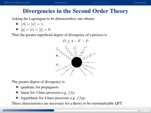
Divergencies in the Second Order TheoryAsking the Lagrangian to be dimensionless one obtains
I [A] = [ψ] = 1,I [g] = [e] = [ξ] = 0.
Thus the greater superficial degree of divergency of a process is
D ≤ 4− F − P
The greater degree of divergency is:I quadratic for propagatorsI linear for 3 lines processes e.g. ffpI logarithmic for 4 lines processes e.g. ffpp
These characteristics are necessary for a theory to be renormalizable QFT.
15 / 37

QFT and NKR formalism Quantization Renormalization Conclusions
Free Parameters and Counterterms (ξ = 0)In terms of the bare parameters m2
b , eb, gb the Lagrangian is
L = −1
4FµνFµν + (∂µ − iebAµ)ψ[gµν − igbMµν ](∂ν + iebAν)ψ −m2
b ψψ.
Introducing the renormalized parameters m2, e y g and the renormalized fields
Aµr = Z− 1
21 Aµ y ψr = Z
− 12
2 ψ there appear the following counterterms
lagrangiano de esta forma es conveniente ya que nos brindara una interpretacion nıtida de dichascondiciones. Cuando pensamos en las reglas de Feynman de la teorıa en terminos de los camposrenormalizados y los parametros ”renormalizados”, las reglas de Feynman aparte de tener losdiagramas de la figura 3.1 deben incluir los siguientes diagramas asociados a los contratermi-nos que se muestran en la figura 4.1, es importante mencionar que estos son introducidos comointeracciones.
p
i(p2 −m2)δZ2 − iδm
q
−i(gµνq2 − qµqν)δZ1
µ ν
p p�
q, µ
−ie [V µ(p�, p)] δe + egMµν(p� − p)νδg
p p�
µ ν
2ie2gµνδ3
Figura 4.1: Reglas de Feynman para los contraterminos
En lo sucesivo no se utilizara el subındice r en las cantidades renormalizadas para ahorrarespacio, pero se mantiene por claridad el subındice d en los parametros desnudos.
4.5. Condiciones de Renormalizacion
Nuestra hipotesis de renormalizacion es que al introducir en la teorıa la informacion de losexperimentos, mediante las condiciones de renormalizacion que a continuacion se presentan, lateorıa queda bien definida a todos los ordenes. Las condiciones de renormalizacion que usaremoscorresponden al esquema sobre las capas de masa. Para motivar estas condiciones empezamosdescribiendo los procesos en los que podemos remover las divergencias utilizando los contratermi-nos (que dependen de los parametros desnudos), estos procesos son: los dos propagadores y losvertices ffp y ffpp.
54
16 / 37

QFT and NKR formalism Quantization Renormalization Conclusions
Dimensional Regularization
Extend the theory to d dimensions. The natural objects to be extended to d dimensionare the Lorentz generators Mµν
[Mαβ ,Mµν ] = −igβνMαµ + igβµMαν − igαµMβν + igανMβµ, with gµµ = d
{Mµν ,Mαβ} =1
2(gµαgνβ − gµβgνα)− i
2εµναβγ5,
e.g. we can use the last expression to calculate to calculate a trace in a fermion loop
tr{MµνMαβ} =f(d)
4(gµαgνβ − gµβgνα) with lım
d→4f(d) = 4,
17 / 37

QFT and NKR formalism Quantization Renormalization Conclusions
Photon PropagatorAs usual one can express the complete photon propagator i∆µν
c (q) as
40 Capıtulo 4. Renormalizacion
donde una vez mas el asterisco (∗) indica que el diagrama se considera sin las lıneasexternas. Es decir, que Π∗µν
L (q) es la contribucion a segundo orden en e a Π∗µν(q).Los unicos tensores con que contamos para aparecer en Π∗µν(q) son gµν y qµqν . Laidentidad de Ward nos dice que qµΠ∗µν = 0, por lo que Π∗µν(q) es proporcional a(gµνq2 − qµqν) y entonces lo escribimos como
Π∗µν(q) = (q2gµν − qµqν)Π(q2). (4.25)
El propagador completo vendra dado por la suma
=−igµν
q2+−igµρ
q2
�(q2gρσ − qρqσ)Π(q2)
� −igσνq2
+ ... (4.26)
=−igµν
q2+−igµρ
q2
�δρν −
qρqνq2
�(Π(q2) + Π2(q2) + ...). (4.27)
Nuevamente la suma de todos los diagramas forma una serie geometrica, por lo que(considerando que los terminos proporcionales a qµ, qν se desvanecen) podemos abre-viar el resultado anterior
−igµν
q2(1− Π(q2)). (4.28)
Vamos a hacer el calculo de Π∗µνL de la ecuacion (4.24), empleamos en esta expresion
el parametro de Feynman x para combinar los dos factores en el denominador
1
AB=
� 1
0
dx
[Ax + B(1− x)]2. (4.29)
Se obtiene
1
(p2 −m2)((p− q)2 −m2)=
� 1
0
dx[(p− qx)2 −m2 + q2x(1− x)]−2. (4.30)
Ahora hacemos el cambio de variable l = p− qx, con lo que el numerador es
2lµlν−gµν l2−2xqµqν(1−x)+gµν(m2+q2x(1−x))+ terminos lineales en l. (4.31)
Los terminos que son lineales en l no contribuyen a la integral por simetrıa, solo loharan las potencias pares. Para estas hacemos el reemplazo lµlν −→ 1
4gµν l2. Hacemos
i∆µνc (q) = i∆µν(q) + i∆µσ[−iΠσρ(q)][i∆
ρν(q)] + ...
where Πµν(q) is the vacuum polarization
Πµν(q) = (q2gµν − qµqν)π(q2),
Then the complete propagator is given by
∆µνc (q) =
−gµν + qµqνπ/q2
[q2 + iε][1 + π].
The first condition of renormalization is that the photon doesn’t acquired mass due tothe radiative corrections, i.e.
π(q2 → 0) = 0.
18 / 37

QFT and NKR formalism Quantization Renormalization Conclusions
Vacuum polarization to one loopIt has the following contributions
−i(gµνq2 − qµqν)π(q)2 = −i(gµνq2 − qµqν)π∗(q2)− i(gµνq2 − qµqν)δZ1
The first renormalization conditions requires
δZ1 = −π∗(q2 = 0),
q,α q, ν q, µ q, ν
l
l + q
l
Figura 4.2: Diagramas de Feynman que contribuyen a la polarizacion del vacıo
por el Lagrangiano (2.49), que parece corresponder al presente formalismo con g = 2. Un resulta-do importante que al parecer ya se habıa obtenido en la literatura es la correccion finita al factorgiromagnetico a un lazo.
4.8.1. Polarizacion del Vacıo
Las dos contribuciones a un lazo para la polarizacion del vacıo Π∗µν(q) estan dadas en lafigura 4.2. Usando las reglas de Feynman de la figura 3.1 se pueden escribir sus respectivascontribuciones
−iΠ∗µν(q) = (−1
2)�
ddl
(2π)dtr
��− ie�Vν(l, l + q)
�� i
�[l + q]
��− ie�Vµ(l + q, l)
�� i
�[l]
�+
�2ie�2gµν
�� i
�[l]
��
= (−12)e2µ4−d
�ddl
(2π)dtr
�Vν(l, l + q)Vµ(l + q, l)�[l + q]�[l]
− 2gµν
�[l]
�
= (−12)e2µ4−d
�ddl
(2π)dtr
� [(2l + q)ν + igMναqα][(2l + q)µ − igMµβqβ]
�[l + q]�[l]− 2gµν
�[l]
�
= (−12)e2µ4−d
�ddl
(2π)dtr
�(2l + q)µ(2l + q)ν + g2MναMµβqαqβ]
�[l + q]�[l]− 2gµν
�[l]
�
= (−12)e2µ4−d
�ddl
(2π)d
�f(d)(2l + q)µ(2l + q)ν + f(d)4 g2(gµνq
2 − qνqµ)�[l + q]�[l]
− 2f(d)gµν
�[l]
�
(4.62)
donde el factor (−12) en la primera expresion aparece debido al lazo fermionico, y usamos las expre-
siones (4.58) para calcular las trazas, esto es tr[MναMµβ] = f(d)4 [gµνgαβ−gνβgµα] y tr{Mνµ} = 0,
como ya se menciono tambien puede usarse (4.60) para obtener estas trazas, el resultado es exac-tamente el mismo. Note que la dependencia en g es explıcitamente invariante de norma, de hecho
62
Finally, imposing the renormalization condition the physical vacuum polarization is
π(q2) =2e2
(4π)2
Z 1
0dx ln
»m2 − q2x(1− x)
m2
– »(1− 2x)2 − g2
4
–,
for g = 2 one recovers the one loop vacuum polarization of the conventional Dirac formalism.
19 / 37

QFT and NKR formalism Quantization Renormalization Conclusions
Charge running in the Ultrarelativistic limit
Due to the quantum effects the classical Coulomb potential modifies as
V (~x) =
Zd3q
(2π)3ei~q·~x
−e2
|~q|2[1 + π(−|~q|2)],
in the ultrarelativistic domain one has an effective charge given by
e2eff =
e2
1 + π(q2 >> m2)= e2
.h1− e2
12π2
`1− 3
2[1− g2
4]´
ln−q2
Am2
i,
where A ≡ exp
(5
3
1− 95[1− g2
4]
1− 32[1− g2
4]
),
Which means that the gyromagnetic factor g impacts the running of the fine structureconstant α(q2)!
20 / 37

QFT and NKR formalism Quantization Renormalization Conclusions
Fermion Propagator
Analogously the complete fermion propagator iSc(p) could be expressed as
iSc(p) = iS(p) + iS(p)[−iΣ(p)]iS(p) + ...
where −iΣ(p2) is the fermion self energy. Adding up the series
Sc(p) =1
p2 −m2 − Σ(p) + iε,
Second renormalization condition: m represents the physical mass of the particle, i.e.the complete propagator has a simple pole at p2 = m2
Σ(p = m2) = 0,∂Σ(p)
∂p2
˛p2=m2 = 0.
21 / 37

QFT and NKR formalism Quantization Renormalization Conclusions
Fermion Self Energy to one loop
The contributions up to one loop are
−iΣ(p2) = −iΣ∗(p2) + i(p2 −m2)δZ2 − iδm,
The second renormalization conditions requires
iδm = −iΣ∗(p2 = m2) δZ2 =∂Σ∗(p)
∂p2
˛p2=m2 ,
p p p p
l
l + pl
Figura 4.3: Feynman diagrams for the fermion self-energy
4.8.2. Autoenergıa del Fermion
Las contribuciones a la autoenergıa de fermion −iΣ∗(p) a un lazo estan dadas en la figura4.3, sus respectivas contribuciones son
−iΣ∗(p) =�
ddl
(2π)d
��− ie�V α(p + l, p)
�� i
�[p + l]
��− ie�V β(p, p + l)
��−igαβ�[l]
�+
�2ie�2gµν
��−igµν
�[l]
��
la ultima integral es cero para d �= 2, como lo muestra la siguiente manipulacion�
ddl
l2 + i0=
�dd(cl)
(cl)2 + i0= cd−2
�ddl
l2 + i0,
el resto de la integral es
−iΣ∗(p) = −e2µ4−d
�ddl
(2π)d
[(2p + l)µ − igMµαlα][(2p + l)µ + igMµβlβ]
�[l + p]�[l]
= −e2µ4−d
�ddl
(2π)d
(2p + l)2 + g2MµαMµβlαlβ
�[l + p]�[l]
para simplificar esta expresion se usan de nuevo (4.56) y (4.56)
2MµαMνβ = [Mµα, Mνβ ] + {Mµα, Mνβ}
= −igαβMµν + igµβMαν − igµνMαβ + igµβMαν +12(gµνgαβ − gµβgαν)− i
2γ5�µανβ
⇒MµαMµβlαlβ =14(d− 1)l2 (4.74)
entonces la autoenergıa del fermion puede escribirse como
−iΣ∗(p2) = −e2µ4−d
�ddl
(2π)d
(2p + l)2 + g2
4 (d− 1)l2
�[l + p]�[l]
= −e2µ4−d
�ddl
(2π)d
4p2 + 4pl
�[l + p]�[l]− e2µ4−d
�ddl
(2π)d
1 + g2
4 (d− 1)�[l]
(4.75)
introduciendo en la primera integral la parametrizacion de Feynman correspondiente (B.1)
1�[l]�[l + p]
=� 1
0dx[�[l](1− x) + x�[l + p]]−2 =
� 1
0dx[(l + px)2 − xm2 + p2x(1− x)]−2,
(4.76)
65
Σ(p2) =α
πp2
Z 1
0
dx(x− 1) ln
»m2x− p2x(1− x)
m2
–− 3αm2
2π− α
π[p2 −m2]
Z 1
0
dx
x.
22 / 37

QFT and NKR formalism Quantization Renormalization Conclusions
ffp VertexThe contributions to the one particle irreducible ffp vertex Γµ(q ≡ p′ − p, r ≡ p′ + p) are
−ieΓµc (p′, p) = −ieV µ(p′, p)− ieΓ∗µ(p′, p)− ieV µ(p′, p)δe − ie[igMµν(p′ − p)ν ]δg ,
4.9. Vertice fermion-fermion-foton a un Lazo
Las contribuciones a un lazo del vertice ffp irreducible de una partıcula estan dadas en lafigura 4.4, sus repectivas contribuciones Γ∗µ(p�, p) = Γ∗µ
1 (p�, p) + Γ∗µ2 (p�, p) + Γ∗µ
3 (p�, p) son
p
l + p l + p�
p�
l
q, µ
p
l
l + p
p� p
l + p�l
p�
Figura 4.4: Diagramas de Feynman a un lazo ffp
−ie�Γ∗µ1 =
�ddl
(2π)d
�− ie�V α(l + p�, p�)
�� i
�[l + p�]
��− ie�V µ(l + p, l + p�)
�� i
�[l + p]
�×
×�− ie�V β(p, l + p)
��−igαβ�[l]
�
= −e�3�
ddl
(2π)d
V α(l + p�, p�)V µ(l + p, l + p�)V β(p, l + p)�[l + p�]�[l + p]�[l]
(4.82)
−ie�Γ∗µ2 =
�ddl
(2π)d[i2e�2gµν ]
� i
�[p + l]
��− ieV β(p, p + l)
��−igνβ�[l]
�
= e�2�
ddl
(2π)d
2V µ(p, p + l)�[l]�[p + l]
(4.83)
−ie�Γ∗µ3 =
�ddl
(2π)d
�− ie�V α(p� + l, p�)
�� i
�[p� + l]
��i2e�2gµν
��−igβν�[l]
�
= e�2�
ddl
(2π)d
2V µ(p� + l, p�)�[l]�[p� + l]
(4.84)
4.9.1. Primera Identidad de Ward a un Lazo
Puede mostrarse que la primera dentidad de Ward (3.63) se satisface a un lazo, contrayendola expresion para el vertice con el momento del foton se obtiene
(p� − p)µΓ∗µ = ie�2�
ddl
(2π)d
�(�[l + p]−�[l + p�])V α(l + p�, p�)Vα(p, l + p)�[l + p�]�[l + p]�[l]
+2qµV µ(p, p + l)
�[p + l]�[l]+
2qµV µ(p� + l, p�)�[p� + l]�[l]
�
67
Evaluating on mass shell
Γ∗µ(p2 = p′2 = m2, q2 = 0) =e2
(4π)2
nh− 2[
1
ε− γ + ln 4π] + 2 ln
m2
µ2− 4
Zdx
x
iV µ(r, q)
+h2 + [1− g2
4][
1
ε− γ + ln 4π − ln
m2
µ2]iigMµνqν −
e2
(4πm)2igMβαrβqαr
µo.
There is a divergency for g 6= 2, this can only be removed assuming that the gyromagneticfactor must be renormalized.
23 / 37
QFT and NKR formalism Quantization Renormalization Conclusions
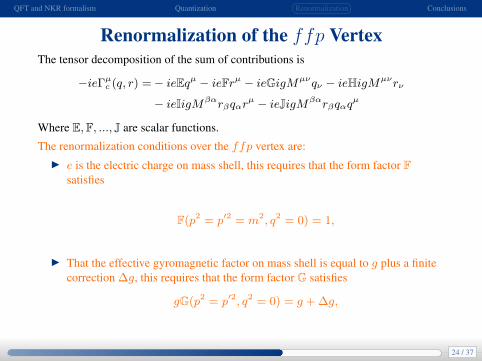
Renormalization of the ffp VertexThe tensor decomposition of the sum of contributions is
−ieΓµc (q, r) =− ieEqµ − ieFrµ − ieGigMµνqν − ieHigMµνrν
− ieIigMβαrβqαrµ − ieJigMβαrβqαq
µ
Where E,F, ..., J are scalar functions.
The renormalization conditions over the ffp vertex are:I e is the electric charge on mass shell, this requires that the form factor F
satisfies
F(p2 = p′2 = m2, q2 = 0) = 1,
I That the effective gyromagnetic factor on mass shell is equal to g plus a finitecorrection ∆g, this requires that the form factor G satisfies
gG(p2 = p′2, q2 = 0) = g + ∆g,
24 / 37

QFT and NKR formalism Quantization Renormalization Conclusions
Renormalized ffp vertex
These renormalizations conditions determine the value of the remaining counterterms
δe =e2
(4π)2
h2(
1
ε− γ + ln 4π)− 2 ln
m2
µ2+ 4
Z 1
0
dx/xi,
δg =e2
(4π)2[g2
4− 1][
1
ε− γ + ln 4π − ln
m2
µ2],
the first expression implies e =√Z1ed.
Introducing these expressions one obtains the ffp vertex at arbitrary momentum(q, r)
−ieΓµc (q, r) =− ieEqµ − ieFrµ − ieGigMµνqν − ieHigMµνrν
− ieIigMβαrβqαrµ + JigMβαrβqαq
µ
25 / 37

QFT and NKR formalism Quantization Renormalization Conclusions
Form Factors
F(r2, q
2, r · q,m) = 1 +
α
4π
n Z 1
0dx(2− x)
hln
∆1(p,mx12 , x)
m2+ ln
∆1(p′,mx12 , x)
m2
i
+
Z 1
0
Z 1−x
0dxdy
h2 ln
m2
∆2(q, r,m, x, y)+q2[( g2
4 − 1)(x + y) + 1] + r2[2(x + y)− (x + y)2 − 1]
∆2(q, r,m, x, y)
+r · q[y − x + x2 − y2]
∆2(q, r,m, x, y)+
4
(x + y)2
io,
G(r2, q
2, r · q,m) = 1 +
α
4π
n Z 1
0dx(
g2
4− 1) ln
∆1(q,m, x)
m2
+
Z 1
0dxx
hln
∆1( q+r2 ,mx
12 , x)
m2+ ln
∆1( q−r2 ,mx
12 , x)
m2
i+
Z 1
0
Z 1−x
0
4dydx
(x + y)2
+
Z 1
0
Z 1−x
0dxdy
h− 2 ln
m2
∆2(q, r,m, x, y)+r2[(x + y)− 1] + (1− g
2 )(r · q)(y − x) + q2
∆2(q, r,m, x, y)
io.
...
26 / 37

QFT and NKR formalism Quantization Renormalization Conclusions
Finite correction to the gyromagnetic factor
The effective gyromagnetic factor on mass shell is given by
−ieΓµc = −ie[G(r2 = 4m2, q2 = r · q = 0)igMµνqν ] + ...,
G(r2 = 4m2, q2 = r · q = 0) = 1 +α
2π.
This equation shows that the finite correction to the gyromagnetic factor to one loopis
∆g =g
2
α
π,
for g = 2 this is just the the conventional result ∆g =α
π!
27 / 37

QFT and NKR formalism Quantization Renormalization Conclusions
ffpp VertexCalculating the ffpp vertex one observes that the divergencies are removed by thepast renormalization conditions
p
p + l
p�
l
p + k + l
p� + l
p + k − p�, νµ, k
p p + l p�
l
p� − k + l
p� + l
µ, k p + k − p�, ν
p p�
p + l p� + l
µ, k p + k − p�, ν
l
p p�
l
p + k + l
µ, k p + k − p�, ν
p p�
l
p� − k + l
µ, k p + k − p�, ν
p p�
l
p + l
p + k + l
µ, k p + k − p�, ν
p p�
l
p + l
p� − k + l
p + k − p�, νµ, k
p p + k + l p�
l
p� + l
p + k − p�, νµ, k
p p + l p�
l
p� − k + l
p + k − p�, νµ, k
Figura 4.5: Diagramas de Feynman para el vertice ffpp a un lazo.
ie�2Λ∗µν1+2 =− e�4
�ddl
(2π)d
V α(p� + l, p�)V ν(p + k + l, p� + l)V µ(p + l, p + k + l)Vα(p, p + l)�[p� + l]�[p + k + l]�[p + l]�[l]
− e�4�
ddl
(2π)d
V α(p� + l, p�)V µ(p� − k + l, p� + l)V ν(p + l, p� − k + l)Vα(p, p + l)�[p� + l]�[p� − k + l]�[p + l]�[l]
(4.120)
ie�2Λ∗µν3 =e�4
�ddl
(2π)d
V α(p� + l, p�)2gµνVα(p, p + l)�[p� + l]�[p + l]�[l]
(4.121)
Λ∗µν4+5 =− e�4
�ddl
(2π)d
� 4gµν
�[p + k + l]�[l]+
4gµν
�[p� − k + l]�[l]
�(4.122)
75
28 / 37

QFT and NKR formalism Quantization Renormalization Conclusions
Perspectives
The rest of superficially divergent processes are (with 3 and 4 external lines)
These processes must be finite if the theory is renormalizable to one loop.
We expect that the first process to be zero due to charge conjugation symmetry.
29 / 37

QFT and NKR formalism Quantization Renormalization Conclusions
Index
Quantum Field Theory and the NKR Formalism
Quantization
Renormalization
Conclusions
30 / 37

QFT and NKR formalism Quantization Renormalization Conclusions
Conclusions
I We studied the one loop renormalization using path integralquantization, obtaining the Feynman rules and showing the Wardidentities to all orders, they were verified to one loop.
I It was shown that the coupling constants are adimensional and that thesuperficial degree of divergency of a given process is bounded by thenumber of external lines.
I By imposing renormalization conditions (that identified therenormalized couplings) it was shown that the divergenciescorresponding to the propagators, ffp and ffpp vertexes are removedfor all g.
I It is remarkable that the Dirac gamma matrixes γµ are not necessarybut natural objects are the Lorentz generators Mµν .
31 / 37

QFT and NKR formalism Quantization Renormalization Conclusions
Conclusions
I Vacuum polatizations to one loop: is gauge invariant, for g = 2 werecover the conventional result. However in general it depends on gwhich means that the running of the fine structure constant α(q2)depends of it. The fermion self energy is independent of g at one looplevel.
I Divergencies corresponding to the ffp vertex for g 6= 2 are onlyremoved assuming that the gyromagnetic factor must be renormalized.
I The finite correction to the gyromagnetic factor which depends on g,and in the case of g = 2 one recovers the correct Schwinger correction.
32 / 37
QFT and NKR formalism Quantization Renormalization Conclusions
Perspectives
I To finish the study of the one loop renormalization for 1/2,
I Tenormalization of the NKR formalism for spin 3/2.
I ¿Generalizations?
33 / 37

QFT and NKR formalism Quantization Renormalization Conclusions
Thanks
34 / 37

QFT and NKR formalism Quantization Renormalization Conclusions
The Reduction Formula S
Consider the S matrix elements
Sαβ = 〈kµ1′ , σ1′ , ..., kνn′ , σn′ ;β, out|pκ1 , σ1, ..., p
θm, σm;α, in〉
reduction formulas allow us to simplify
Sαβ =Z121′ ...Z
12m
Xlili′
Zdx1′ ...dxm
ˆul1′ (x1′ , p1′ , σ1′)...uln′ (xn′ , pn′ , σn′)
˜〈0|T (φl1′ (xl1′ )...φlm(xlm))|0〉
ˆul1(x1, p1, σ1)...ulm(xm, pn′ , σm)
˜I 〈0|T (φl1′ (xl1′ )...φln′ (xln′ )φl1(xl1)...φlm(xlm))|0〉.I φi(xi) with quantum numbers {pνi , σi} corresponding to in or out,
I Zi field strength renormalization of φi,
I ui(xi, pi, σi) differential operators acting in φi(xi).
To study the renormalization we focus on calculating 〈0|T (φ...)|0〉 .
35 / 37

QFT and NKR formalism Quantization Renormalization Conclusions
Free Parameters and Counterterms (ξ = 0)In terms of the bare parameters m2
d, ed, gd the Lagrangian is
L = −1
4FµνdFdµν + (∂µ − iedAdµ)ψd[gµν − igdMµν ](∂ν + iedAdν)ψd −m2
dψdψd.
Introducing the renormalized parameters m2r , er y gr and the renormalized fields
Aµr = Z− 1
21 Aµd y ψr = Z
− 12
2 ψd the Lagrangian is
L =− 1
4Fµνr Frµν −
1
2(∂µArµ)2 − 1
4Fµνr FrµνδZ1 −
1
2(∂µArµ)2δZ1
+ ∂µψr∂µψr −m2rψrψr + [∂µψr∂µψr −m2ψrψr]δZ2 − δmψrψr
− ier[ψrTrνµ∂µψr − ∂µψrTrµνψr]Aνr − ier[ψrTrνµ∂µψr − ∂µψrTrµνψr]Aνr δe− ier[ψr(−igrMνµ)∂µψr − ∂µψr(−igrMµν)ψr]A
νr δg + e2rψrψrA
µrArµ
+ e2rψrψrAµrArµδ3,
where
δZ1 ≡ Z1 − 1 δZ2 ≡ Z2 − 1 δm ≡ Z2[m2d −m2
r],
δe ≡ed
erZ
121 Z2 − 1 δg ≡
ed
erZ
121 Z2[
gd
gr− 1], δ3 ≡
e2de2rZ1Z2 − 1
36 / 37

QFT and NKR formalism Quantization Renormalization Conclusions
Dimensional Regulatization
We could use the conventional extension
{γµ, γν} = gµν with gµµ = d,
tr{γµ} = 0, trI =f(d) with lımd→4
f(d) = 4,
Mµν =i/4[γµ, γν ].
but the gammas γµ are not necessary we could use instead only the Lorentzgenerators Mµν
[Mαβ ,Mµν ] = −igβνMαµ + igβµMαν − igαµMβν + igανMβµ, con gµµ = d
{Mµν ,Mαβ} =1
2(gµαgνβ − gµβgνα)− i
2εµναβγ5 con trγ5 = 0, (γ5)2 = 1,
trMµν = 0, tr{MµνMαβ} =f(d)
4(gµαgνβ − gµβgνα) con lım
d→4f(d) = 4,
37 / 37
Recommended
![arXiv:1310.4507v2 [cond-mat.str-el] 5 Feb 2014 fileBifurcation in entanglement renormalization group ow of a gapped spin model Jeongwan Haah1,2 1Department of Physics, Massachusetts](https://img.pdfslide.us/doc/110x75/5e11bd693933dc7ce00c58e3/arxiv13104507v2-cond-matstr-el-5-feb-2014-in-entanglement-renormalization-group.jpg)