Relocation of Public Sector Workers:
The local labour market impact of the Lyons Review
Giulia Faggio*
July 2013
* Spatial Economics Research Centre (SERC), London School of Economics (LSE). Address: Houghton
Street, London WC2A 2AE, United Kingdom; e-mail: [email protected]; Tel.: +44-20-7852-3555
Acknowledgements: I would like to thank Steve Gibbons, Alan Manning, John Morrow, Henry
Overman, Steve Pischke, Olmo Silva, William Strange and participants at the SERC work-in-progress
seminar and the CEP labour market workshop at LSE for comments and suggestions. I am responsible
for any errors or omissions.

Relocation of Public Sector Workers:
The local labour market impact of the Lyons Review*
Abstract
This paper assesses the local labour market impact of a UK public sector relocation initiative labeled the
Lyons Review. The review resulted in the dispersal of more than 25,000 civil servants out of London and
the South East towards other UK destinations. The objective of the paper is to detect whether inflows of
public sector jobs have crowded out private sector activity or stimulated the local provision of additional
jobs in the private sector. By applying a difference-in-difference approach, I evaluate the policy impact
comparing areas in close proximity to a relocation site with areas further away. I find that the dispersal of
public sector workers that followed the implementation of the Lyons Review had a positive impact on
local services with a negative, but weaker, impact on manufacturing.
JEL classification: O1, R23, R58, J61
Keywords: Economic development; regional labour markets; regional government policy; job
displacement
* This work was based on statistical data from the ONS that are Crown copyright and reproduced with the
permission of the controller of HMSO and Queen's Printer for Scotland. The use of the data in this work does not
imply the endorsement of ONS or the Secure Data Service at the UK Data Archive in relation to the interpretation
or analysis of the data. This work uses research datasets which may not exactly reproduce National Statistics
aggregates.

2
1. Introduction
Governments design a variety of place-based policies attempting to reverse the fate of
economically declining areas and create employment opportunities for local residents. In the US,
Enterprise and Empowerment Zone programmes spur the creation of jobs by providing tax
incentives to businesses located in designated areas.2 Similarly, French Enterprise Zone programmes
are targeted at discretely bound areas. The UK government follows a slightly different approach by
designing either place-based policies with no-predetermined spatial scale (the Single Regeneration
Budget programme), or spatially-bound policies whose funding goes indirectly to businesses through
local government (the Local Enterprise Growth Initiative)3. The UK government also uses relocation
programmes of public sector workers to address regional employment problems and to reduce spatial
disparities in income. Strictly speaking, relocation programmes of public sector workers are not
‘pure’ place-based policies. They address a variety of objectives, including delivering cost savings,
re-organising the government estate, and enhancing devolution.
When a public sector job is created in an area, it may have a local ‘multiplier effect’: It may
create additional local jobs as a result of the increased demand for locally produced goods and
services. Conversely, a rise in public sector employment may trigger general equilibrium effects in
the form of higher local wages or higher housing prices (see Moretti, 2011; Faggio and Overman,
2013). These general equilibrium effects may be stronger than the multiplier effect and result in a
crowding out or displacement of local businesses.
The debate on the use of public sector worker relocations as a tool to boost regional
development is not new. The UK first government-sponsored review was commissioned in the 1960s
(Flemming Review, 1963), followed by the Hardman Review (1973) and by the Lawson-Thatcher
Review (1988). Notwithstanding the attention given by the government to the subject, there is scarce
evidence of the effects of a public sector relocation programme upon local labour markets. This
study tries to fill this gap by assessing the local labour market impact of a public sector relocation
initiative labelled the Lyons Review.
In 2004, Sir Michael Lyons led a UK government-sponsored independent study on the scope
for public sector relocations out of London and the South East towards other UK destinations. The
2 See, for recent evaluations of the US programmes, Neumark and Kolko (2010) and Busso, Gregory and Kline (2013).
3 See Gibbons, Overman and Sarvimäki (2011) and Einio and Overman (2012) for evaluations of the SRB programme
and the LEGI initiative, respectively.

3
review proposed a relocation of about 20,000 civil servants within a six-year period. Thanks to the
adoption of effective ‘push’ factors (such as relocation targets and property controls), the original
target was delivered nearly a year ahead of schedule. By March 2010, the program had relocated
more than 25,000 jobs. The 2004 relocation programme addressed a variety of objectives including
the government desire to stimulate economic activity in less-prosperous areas and, thus, reducing
spatial imbalances between London and periphery areas. To the extent that the relocation programme
had any impact on local economic conditions, this paper aims to detect the causal effects of the
intervention.
In order to detect any causal impact, I use panel data at a detailed geographical scale (Census
2001 Output Areas) covering years before and after the implementation of the programme. Adapting
the approach from Gibbons, Overman and Sarvimäki (2011), I construct a measure of treatment
intensity that is a non-parametric function of the distance to a relocation site. This approach also
provides a parsimonious way to deal with multiple sites. In other words, I assume that effects are
additive and vary by distance. My objective is to evaluate the effect and intensity of the treatment by
comparing areas in close proximity to a relocation site with areas further away. In order to do that, I
apply a difference-in-difference estimation approach and look at the changes in outcome across areas
before and after the implementation of the programme. In the main analysis, I compare neighbouring
areas that are similar in terms of initial economic and demographic characteristics.
This study finds that the dispersal of public sector workers that followed the implementation
of the Lyons Review (2004) had a small positive impact on local services and a negative, but
weaker, impact on manufacturing. Results seem robust to a series of robustness checks: including
pre-trends in the estimation; conducting a placebo experiment and looking at the impact of the
relocation programme on (1998-2002) variation in outcomes; and testing for causality in the spirit of
Granger (1969). Furthermore, the analysis is extended to measure the contribution of yearly
relocations to total 2003-2008 variation in outcome; to test whether bigger relocations are associated
with a larger policy impact; and to explore which demand channel (either consumer demand or
intermediate demand) is more likely to explain the positive impact on services. Two robustness
checks based on modified versions of spatial differencing conclude the analysis.
This paper makes an original contribution to the literature on the dispersal of public sector
workers. To my knowledge, no previous study has looked at the local impact of a public sector
relocation programme using a difference-in-difference approach and fine spatial scale data as

4
presently available. Previous out-of-London relocation studies have focused on the financial costs
and benefits of the moves (see, among others, Goddard and Pye, 1977; Ashcroft et al., 1988;
Marshall et al., 1991; Deloitte, 2004); some have provided descriptive evidence usually based on
interviews with internal managers responsible for implementing relocations and/or secondary data
sources (see Marshall et al., 2003; Experian, 2004); others have used regional input-output models4
aimed at ex-ante predicting the local multiplier impact of proposed dispersals (see Ashcroft and
Swales, 1982a and 1982b; Ashcroft et al., 1988; Experian, 2004).
Furthermore, the debate on public sector relocation is not limited to the UK.5 Little attention,
however, has been paid in previous research to estimate the local labour market impact of a
relocation programme. Faggio and Overman (2013) made a first step in the right direction by
looking at the impact of public sector employment on local labour markets. They use fairly detailed
geographical information on 352 English LAs and look at changes in total public sector employment
during the period 2003-2007, but they do not analyse the local impact of a relocation programme.
Interestingly, they find that public sector employment does not have any impact on total private
sector employment at the LA level. They do find, however, that public sector employment impacts
the local composition of private sector jobs.
A recent paper by Becker, Heblich and Sturm (2012) looks at the rise of Bonn as the new
federal capital of Western Germany at the end of World War II. Becker et al. (2012) investigate how
this historic public sector relocation from Berlin to Bonn changed the local economic structure of the
new capital relative to other cities of similar initial size and demographic characteristics. They find
limited effects given the extent and relevance of the relocation.
This paper also contributes to the growing literature on the evaluation of place-based
government policies. As also noted by Einio and Overman (2012), earlier studies were impaired by
the problem of non-random placement6. Later studies have combined data at a finer spatial scale
with well-designed identification strategies to overcome the problem of causal inference in non-
experimental settings. In the US, Enterprise and Empowerment Zone programmes have been
successfully evaluated by Neumark and Kolko (2010); Busso and Kline (2008); and Busso, Gregory
4 There is an extensive literature on regional input-output models. See Miller and Blair (2009) for a textbook reference
and Faggio and Overman (2013) for a discussion in this context. 5 See, among others, Daniels (1985), Clarke (1998), and Guyomarch (1999) for France; Cochrane and Passmore (2001),
Haeussermann and Kapphen (2003) for Germany; Myung-Jin Jun (2007) for Korea. 6 As pointed out by the literature on program treatment effects (see Heckman, LaLonde and Smith, 1999; DiNardo and
Lee, 2011), the problem of causal inference in non-experimental evaluations can be substantial.

5
and Kline (2013). Other less well-known programmes, like the New Market Tax Credit, have also
been carefully evaluated (see Freedman, 2012 and 2013). In Europe and the UK, evaluations of the
French Enterprise zone programmes, the UK LEGI and the UK Single Regeneration Budget stand
out for accuracy.7
The remainder of the paper is structured as follows: Section 2 provides background on the
relocation program, Section 3 discusses a simple conceptual framework and Section 4 introduces the
empirical strategy. While Section 5 describes the data used, Section 6 presents the main results.
Section 7 concludes.
2. The institutional setting
In 2004, Sir Michael Lyons led a government-sponsored review on the scope for relocating
central government activities out of London and the South East to more peripheral regions. The
review proposed the dispersal of about 20,000 civil service jobs within the six-year period ending in
March 2010. The programme developed very strong ‘push’ factors (such as relocation targets and
property controls) to drive posts out of London at an early stage. Such targets were agreed with
departments as part of the review process. Each department was then accountable for delivering its
own target by March 2010. Property controls stipulated that any government agency wishing to
extend the government’s property commitment in London or in the South East submit a formal
business case for approval. This requirement changed expectations across government: departments
needed to justify their presence in London on the grounds of business needs. Thanks to these push
factors, the original target was delivered nearly a year ahead of schedule. By its end, the programme
relocated more than 25,000 jobs.
The Lyons Review had, among others, several main objectives: delivering cost savings to
taxpayers by reducing accommodation and labour costs; allowing the modernization of public
services; enhancing devolution; and reversing regional decline.
Property costs tend to be higher in London than elsewhere in the country and, most crucially,
14 per cent of government offices (25 per cent of national expenditure) are located in the prime-cost
area of Central London (see Smith, 2010). Despite the national pay scheme, public sector wages also
7 See Gobillon, Magnac and Selod, 2012; Mayer, Mayneris and Py, 2011; Einio and Overman, 2012; Gibbons, Overman
and Sarvimäki, 2012.

6
tend to be higher in London than in the rest of the UK because of the London weighting allowance.
Due to the allure of private sector job opportunities, there are higher retaining and turnover costs.
In the Expedian (2004) report (which provides background research for the Lyons Review),
relocation is also described as a catalyst for re-organising public services and adopting a
performance-driven culture across government departments. It is not accidental that the Lyons
Review recommendations were implemented as a strand of the Gershon Efficiency Review (2004)
whose primary objective was civil service modernisation.
The primary government benefits of devolution, namely reducing cost pressures and
relieving spatial constraints, moves hand in hand with the public benefits of important central
government organs being close to the people, increased confidence and transparency in government
decisions; and an increased sense of belonging. An additional purpose of public sector relocation is
to boost regional growth in UK peripheral areas in an attempt to correct the spatial imbalance
between a rich South-East and less prosperous regions in the North and the West. This study is about
evaluating the programme in light of its ability to achieve this last objective.
Larkin (2010) noted that the size of the government’s relocation programme was fairly small.
Over the period 2004-2010, the programme dispersed 25,420 jobs out of London and the South
East8. This figure represents about 5 per cent of total civil service employment (full-time equivalent)
working in Britain before the relocations began (Civil Service Statistics, 2003). 5 per cent is not a
large number. Looking at the statistics in context, however, reveals that less than one fifth of all civil
servants worked in the capital in 2003 and over 70 per cent worked outside London and the South
East. Therefore, the programme relocated about 20 per cent of all government jobs initially housed
in London or around 17 per cent of those in London and the South East. These are no trivial figures.
What is certainly more interesting is the average number of jobs that successful Local
Authorities (LAs) managed to attract under the relocation process. Out of 408, 116 LAs attracted on
average 670 jobs with a standard deviation of around 520. The dispersion is large: those 116 LAs
received between 1 and 1,600 full-time equivalent jobs. At the 2001 Census Output Area level,
which is the detailed level of geography used in the present paper, the average number of jobs
relocated in receiving Output Areas (OAs) was 270 with a standard deviation of 348. 282 OAs (out
8 I could collect information on the original locations of 20,550 jobs (out of 25,420). While 82 percent of these moves
were out of London, 18 per cent were out of the South East region.

7
of about 160,000)9 were chosen as the preferred destination of between 0.5 and 1276 full-time
equivalent civil service jobs.
When reading background documentation to the Lyons Review (see, e.g., Experian, 2004;
Deloitte, 2004), it is not clear why some destinations were chosen instead of others. Experian (2004)
recommended the government ‘not to choose a building just because is available’, thus suggesting
that this might have been the case in past relocations. In addition, it also recommended to phase staff
moves in manageable chunks, again endorsing the idea of choosing buildings with a long-run
perspective. Furthermore, limited information is available on how relocation decisions were made.
Although the Office of Government Commerce (OGC) had the overall responsibility to rationalise
the civil service estate and oversee departmental relocations, each individual department was
accountable for managing its own relocation programme, including filling posts that were
transferred, or created, in the new location.
As documented in Smith (2010), the implementation process lacked transparency: there was
no government strategic or unified framework according to which all relocation decisions should
have been made. Since coordination across departments was not emphasised, each department
sought to maximise its own business interest and not the Exchequer’s wider objective. Even within
departmental families, departments did not take direct responsibility for the location choices of their
own agencies and Non-Departmental Public Bodies (NDPBs).
An additional point of concern (see Larkin, 2010; Smith, 2010) is the amount of public
resources used by UK Local Authorities in attracting public sector relocations. Again, information
regarding potential destination sites was not collected and made available to all departments in a
transparent way. On the contrary, relocation decision-making was open to marketing campaigns
(often generic) of individual cities. Finally, there is no central record of how many workers actually
moved with the posts and there are no details of relocations packages offered, compensations taken
or incentives given. The Smith Review (2010), which followed in the footsteps of the Lyons Review,
indicates that lack of planning and transparency resulted in higher-than-expected upfront relocation
costs.
As a preliminary way of looking at the relocation data, I collect information on pre-treatment
(2003) characteristics of Local Authorities in England, Wales and Scotland (see Faggio and
9 Output Areas are very small geographical areas built from clusters of adjacent unit postcodes. See Section 5 for further
details.

8
Overman, 2013)10
. Geocoding the location of relocation sites, I associated relocation sites with the
corresponding Local Authorities. I then distinguish between LAs chosen as actual relocation
destinations, LAs not chosen, and LAs in London and the South East from which all relocations
originated. Overall, there is a remarkable similarity between LAs chosen and LAs not chosen as a
relocation site (see Table 1) giving some support to the idea that the relocation sites might be
considered ‘almost randomly assigned’. Looking at demographic variables, educational shares are
very similar (almost identical) between these two groups of LAs. Conversely, there is a higher
proportion of college graduates and a lower share of people with no qualification in London and the
South East11
.
Contrary to expectations, actual relocations are in LAs with a higher initial share of public
sector employment. If anything, I would expect additional public sector jobs to go to areas with a
limited public sector presence. Relocations are also in areas with higher unemployment rates;
slightly higher inactivity rates; and a lower share of entrepreneurial activity.
Looking at political variables (see Table 1), the share of Labour votes at the 1983, 1997 and
2005 general elections is consistently higher (although not statistically different) for the group of
LAs chosen as a relocation site as opposed to the group of LAs not chosen. In addition, support for
Labour seems to grow over time within the group of chosen LAs.
Finally, as I restrict the analysis to the 352 LAs in England for which the 2004 Index of
Multiple Deprivation (IMD) is available 12
, a larger proportion of deprived areas are within the group
of LAs chosen as opposed to the other group. Nevertheless, there were a considerable share (31%) of
deprived areas that were not chosen as a relocation site.
Overall, descriptive statistics presented so far show an important similarity between the two
groups of LAs (chosen and not chosen), thus suggesting that the problem of non-random placement
of this relocation exercise might not be as serious as initially appeared.
10
LA data are retrieved from BIS Local Authority data (2003-2007); ABI Local Authority data (2003-2007); Local Area Labour
Force Survey (1999-2003); ONS Model-based Estimates of Unemployment (1999-2007); Land Registry data (2000-2010); 2004 Index
of Multiple Deprivation statistics. Shares of labour votes at the 1983, 1997 and 2005 elections as well as real mix-adjusted house price
index have been kindly provided by Christian Hilber and Wouter Vermeulen. 11 By conducting a simple T-test on the equality of means, educational shares are not significantly different between the
groups of potential and actual relocation areas. 12
The IMD index identifies the poorest LAs in England ranking areas from least deprived to most deprived according to
six social and economic dimensions.

9
3. Conceptual Framework [Incomplete – Please skip this part]
On pure economic grounds, place-based policies do not appear fully justifiable (see Glaeser
and Gottlieb, 2008). As the government relocates economic activity into unproductive areas, spatial
equilibrium considerations suggest that local residents may not truly benefit from the policy. They
could find themselves in a new equilibrium characterised by higher wages and higher prices
(including housing prices)—all feeding through to a possible higher cost of living.
Obviously, there are differences between moving jobs or workers in terms of local supply
and demand for labour in the destination area. As the public sector expands, the local demand for
labour also expands. If workers move with jobs, the local supply expands with the demand with no
(or little) impact on local wages. Sure, the public sector could open additional vacancies in the new
area attracting local workers who are unemployed or employed somewhere else (assuming complete
mobility of workers across sectors within an area but no mobility across areas). In addition, the
effect on local wages could be complicated by the existence of a national pay scheme: the higher
wage earned in the public sector would draw an increasing number of workers out of the private
sector and into the public sector.
If workers do not move with jobs, the local supply does not expand with the demand creating
upward pressure on local wages (again, there is no mobility across areas). In order to keep labour
costs down, private sector employers (mainly in tradable goods) will be tempted to leave the area.
Private sector workers might then choose whether to follow their current employer outside the area
or search for a new job inside the area (either private or public). As in the previous case, higher
wages in the public sector guaranteed by a national pay scale would attract workers in the public
sector.
In the former case, public sector employment would crowd out private sector employment if
a national pay scheme kept public sector wages artificially high or the public sector offered
additional vacancies expanding its local presence even further. In the latter case, general equilibrium
considerations would already encourage tradable sector employers to leave the area. Again, higher
public sector pay might pull high quality private sector workers into public employment and push
private businesses out of the area.
If I relax the assumption of no worker mobility across local labour markets, workers will
come from adjacent labour markets in response to an upward pressure on wages brought about by an
inflow of public sector jobs (not workers) in to the area or by additional public sector local

10
vacancies. Yet, it is reasonable to suggest that longer term higher public sector salaries do create a
local distortion that works against the private sector.
4. The Empirical Strategy
There are methodological problems associated with ex-post evaluations and the two concepts
of additionality and deadweight may be the most challenging of them. Additionality refers to the
‘amount of output from a policy as compared with what would have occurred without the
government intervention’ (HM Treasury, 1988). Expressed otherwise, additionality would require to
answer the following question: what would have happened in a situation in the absence of a
particular policy intervention or measure? Needless to say, it is impossible to know what would
happen in any of the chosen locales had they not been allocated any public sector jobs. In the
literature (see Heckman et al.,1999, DiNardo and Lee, 2011), a way of solving this additionality
problem is by comparing treated sites with a suitable control group.
The related concept of deadweight can be defined as ‘that part of a public expenditure
programme which is taken up by recipients other than those to whom the expenditure should, if
possible, be directed…’ (HM Treasury, 1988). Some amount of deadweight is inevitable in every
policy intervention. Often is it difficult to evaluate the extent of the loss. Special forms of
deadweight are displacement and crowding out. For instance, businesses might decide to relocate in
the proximity to a treated site where the demand is higher, pulling up employment in nearby areas
and down in areas further away (displacement effect).13
Alternatively, public sector employment
might put upward pressure on local wages forcing local businesses to move out of the areas into less
costly locales (crowding out effect). Evaluating the extent of additionality, crowding out and
displacement are the main issues of this paper.
My ex-post evaluation has additional methodological challenges. Firstly, I deal with places
instead of people (see Glaeser and Gottlieb, 2008; Einio and Overman, 2012, for a discussion). It is
typically harder to identify suitable control groups for places rather than individuals: detailed
geographical level statistics are not easy to find. In addition, area-based policies raise questions
about ‘people versus area’ effects. When investigating a place-based policy, we are often interested
in detecting its impact on the people originally living or working in the area. Unfortunately, area
13
Displacement refers to the extent to which the generation of a desirable outcome in one area leads to a loss of the same
output in another areas.

11
level statistics may be contaminated by people leaving the treated areas during the implementation of
the policy; thereby reflecting both the change in neighbourhood composition and the extent of any
policy impact.
Secondly, it is hard to measure the causal impact of interventions that are not randomly
assigned (see DiNardo and Lee, 2012). Recent studies (see, e.g., Busso and Kline, 2008; Busso,
Gregory and Kline, 2013; Neumark and Kolko, 2010; Einio and Overman, 2012) have successfully
combined empirical strategies, such as spatial differencing as well as comparing earlier and later
rounds of specific policies, with institutional details for helping identification. In this study, limited
information is available on how government selected relocation sites. The little we know is that
relocations were implemented outside a unified framework (Smith, 2010). Coupled with this, the
similarity (documented in Section 2) between areas chosen as relocation sites and areas not chosen
suggest that the non-random nature of this relocation exercise might not be as severe as initially
thought. Furthermore, the difference-in-difference approach used in the present study deals with
time-fixed area unobservables (but not time-varying shocks).
A third methodological challenge is the fact that the spatial scale of the potential treatment
effect is not known a priori. I can identify relocation sites at the level of a postcode, but I do not
know the spatial impact of the relocation. On one hand, the effects of creating additional public
sector jobs may be very localised to the point of impacting only the persons previously working in
the chosen building. On the other hand, they might spread across several kilometres, when they
stimulate additional activity in terms of public workers’ intermediate demand for consultancy and
legal work or final demand for catering and personal services. Furthermore, crowding out and
displacement effects might operate: public sector employment might crowd out local activity in the
receiving areas or it might cause businesses in outlying areas to displace themselves and relocate
into the local area. Finally, locations might be affected by multiple relocations further complicating
the picture.
Using a difference-in-difference approach, this study investigates the impact of treatment
intensity variables on the outcome focusing on locations with similar pre-treatment observational
characteristics used as control group. Consider the estimation equation:
∆�� = ∑ ���∆��
��� + ∑ � ��,����(������)
� + ∆�� (1)
12
where ∆��is the log change in the outcome measure of interest over the period 2003-2008 in a
Output Area i. ��� is a binary indicator for OA i and buffer or control ring c, equal to 1 if the OA has
at least one relocation site within distance c and equal to 0 otherwise. All buffers have a 1km width.
∆��� refers to the total number of jobs moved (i.e., the size of government relocations) an OA faces
in control ring c. Alternatively, I assume equal size across all relocations (i.e., ∆��� = �) so that the
binary indicators ��� are also used as treatment intensity variables. To be precise, ∆��
� (when allowed
to vary) refers to the change in the number of public sector jobs moved between March 2003 and
December 2007.14
Since I consider the cumulative dispersal of public sector workers between 2003
and 2007, this variable was clearly zero for all OAs in 2003 and turned positive for some OAs in
2007. ∑��,���� refer to a set of pre-treatment area controls that may include economic activity of
residents, industry and occupation structures, age of residents, population density, education shares,
household size and dwelling characteristics.15
�� is an error term. All specifications also include
Travel-To-Work-Area (TTWA) fixed effects and observations are clustered at the TTWA level.
Adapting the approach from Gibbons, Overman and Sarvimäki (2011), I estimate the impact
for several treatment intensities defined as a non-parametric function of the distance to a relocation
site. I proceed as follows: I split Britain into about 190,000 census Output Area, which is the unit of
observation chosen for the analysis (see Section 5 for more details); I measure the centroid of each
OA; I compute the Euclidean distance between each government relocation site and all OA centroids
(both expressed in National Grid references); I then compute 1km-wide buffers from each OA
centroid and count the number of relocations in each buffer. In doing so, I make the assumption that
the effects are additive. I then measure the treatment intensity as an interaction of distance with the
size of the relocation, where size refers to the number of jobs moved.
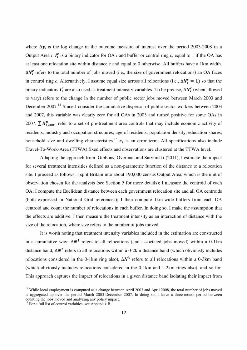
It is worth noting that treatment intensity variables included in the estimation are constructed
in a cumulative way: ∆�� refers to all relocations (and associated jobs moved) within a 0-1km
distance band, ∆�� refers to all relocations within a 0-2km distance band (which obviously includes
relocations considered in the 0-1km ring also), ∆�� refers to all relocations within a 0-3km band
(which obviously includes relocations considered in the 0-1km and 1-2km rings also), and so for.
This approach captures the impact of relocations in a given distance band isolating their impact from
14
While local employment is computed as a change between April 2003 and April 2008, the total number of jobs moved
is aggregated up over the period March 2003-December 2007. In doing so, I leave a three-month period between
counting the jobs moved and analyzing any policy impact. 15
For a full list of control variables, see Appendix B.

13
that of all other relocations. A graphical representation, also adapted from Gibbons, Overman and
Sarvimäki (2011), helps clarify. Consider two Output Areas, area A and area B, and two relocation
sites, site 1 and site 2 (see Figure 1). Remember that buffers or control rings are constructed around
OA centroids and not around relocation sites. If I consider only three 1km-wide buffers, the three
treatment intensity vectors in this graphical representation are: ∆��= (0,1); ∆��= (0,1); ∆��= (2,1).
Looking at equation 1, � are the parameters of interest. Time differencing removes OA
fixed effects that may be correlated with outcomes, meaning that the OLS estimates of � are robust
to time invariant unobserved heterogeneity at the OA level. However, time variant unobserved
heterogeneity at the OA level could still affect the results. In other words, equation 1 will provide
consistent estimates of the treatment variables as long as, conditional on initial characteristics,
unobserved OA level trends in the outcome variables are uncorrelated with the treatment intensity
variables. Even with a very rich set of pre-treatment variables, this condition is unlikely to hold.
An emerging literature16
uses spatial differencing as an initial way to solving this problem.
Spatial differencing (i.e., measuring the difference between an area and its neighbour) removes
unobserved factors that are common across neighbouring sites and attempts to reduce the bias if
these unobservable characteristics are not common but vary across space.
In a standard framework, spatial differencing would, for instance, require to choose two
distance thresholds (d1 and d2, with d2> d1) – defined both as distances to a relocation site– and
restrict attention to compare treated areas within d1 of a relocation site and untreated areas, those
between d1 and d2. Considering how I construct my treatment intensities, as buffers around OA
centroids and potentially reflecting the impact of multiple relocation sites, my empirical strategy
already compares areas in close proximity to a relocation site with areas increasingly further way.
This comparison is done in a consistent way, kilometre after kilometre (within a TTWA). In
principle, equation 1 could include all treatment intensities from 1km distance (to a relocation site)
to 50km distance and each treatment intensity would pick up the impact of relocations on outcomes
in a given control ring. In practice, this over-parameterisation would not be necessary. Partly, it will
not be needed if effects are very localised. Partly, equation 1 could simply include the first 5km or
10km or 15km treatment intensities and then a cumulative treatment intensity variable picking up the
policy impact from 6km (or 11km or 16km) to 50km.
16
Recent papers have successfully used spatial differencing in evaluating the impact of place-based policies in the US
(Neumark and Kolko, 2010; Busso, Gregory and Kline, 2013) and the UK (Gibbons, Overman, Sarvimäki, 2011; Einio
and Overman, 2012).

14
5. Data Construction
This study uses three data sources: Government relocation data provided by the UK Office of
Government Commerce (OGC)17; the Business Structure Database (BSD); and the UK 1991 and
2001 Censuses of Population.
The Government relocation data are comprehensive: They list the total number of actual job
moves within government departments following the implementation of the Lyons Review (2004).
They provide information on 25,408 public sector jobs relocated out of London and the South East
into peripheral UK destinations between June 2003 and December 2010. The data give details on the
date of the move; the government department and business unit involved; the origin or exporting
address of the building from which a job was relocated; and the destination or importing address of
the building receiving the job.
Not all public sector workers were involved, but only those civil servants working for central
government (including government departments, non-ministerial departments and executive
agencies) or for special entities called executive Non-Departmental Public Bodies (NDPBs). UK
NDPBs are, for instance, the Care Quality Commission or the Competition Commission18.
In a substantial number of cases, the geographical information on origin and destination
addresses was missing or misreported. I checked every address in the dataset and filled out the
postcodes when missing, using old government archives, internet search engines and government
agency websites. Since staff moves were phased in manageable chunks, I could identify 1,486
distinct relocations (involving more than 25,000 jobs)19
defined by a precise moving date, the
number of jobs moved, a government department, a business unit, and a destination address. The
majority of these locales were in England (1126), followed by Wales (222), Scotland (119), and
Northern Ireland (19). Given the limited numbers of relocations into Northern Ireland and the usual
17
When the Coalition Government came to power in May 2010, the OGC was dismantled and its main functions
became part of the Efficiency and Reform Group at the Cabinet Office. 18
The Lyons Review (2004) gave guidance for the dispersal of civil servants working in government departments (such
as HM Treasury or Department of Health); non-ministerial department (such as Food Standard Agency or Ofsted);
executive agencies (many of which provide service to the citizens, such as Jobcentre Plus and HM Courts Service); and
executive Non-Departmental Public Bodies (NDPBs). Face-to-face public services not provided directly by central
government, such as those in health (NHS) trusts, schools, police forces, local authorities were outside the scope of the
review. For the rest of the paper, I use government departments as synonymous for central government without making
any distinction between the types of public entities considered by the review. 19
The total number of relocations is 1,522, but 36 destination postcodes were not identified.

15
difficulties in collecting good quality data for this country, I exclude Northern Ireland from the final
sample, which consists of 1,467 relocations, involving about 24,950 job moves within 20
government departments. The bulk of these changes (about 64% of relocations and about 65% of job
moves) occurred between June 2003 and December 2007.
It is worth noting two things: Firstly, my analysis focuses on destination areas. It is clearly
much more interesting to investigate what happens in areas receiving the additional public sector
jobs than knowing what might have happened in the capital where there are buoyant private sector
opportunities easily filling up vacant buildings as they appear. Secondly, it proved much harder to
identify the exact postcodes in London or the South East where jobs originates. Out of 1522, 407
relocations report no geographical detail. Thirdly, the data provides information on the number of
jobs (not workers) moved. I do not know whether a worker who filled the job in London (or in the
South East) actually moved with the relocated job20
. What I do know is that a public sector job was
reduced in the capital while an additional public sector job was created in a peripheral area.
The second database I use is the Business Structure Database (BSD), which provides an
annual snapshot (taken in April at the closing of the fiscal year) of the Inter-Departmental Business
Register (IDBR). The IDBR consists of administrative data collected for revenues and taxation
purposes and is constantly updated. Any business liable for value-added taxation (VAT) and/or with
at least one employee registered for tax collection will appear on the IDBR. For the year 2012, the
VAT threshold for registration was a turnover of taxable goods and services of £77,000, thus
suggesting that the BSD might not sample small and very small businesses. Nevertheless, the ONS
estimated that for 2004 the businesses listed on the IDBR accounted for approximately 99 per cent of
economic activity in the UK.
The BSD data contains information on about 2.4 million business establishments per year
over the period 1997-2011 and includes information on each business’ date of birth, date of death,
postcode, sector of activity (up to 4-digit Standard Industry Classification (SIC) 2003 code) and total
employment. 21
Using the postcode, I assign each local unit active in England, Wales and Scotland to
a Census 2001 Output Area.
20
Civil servants were firstly asked to move with the job. If they did not agree, they could either accept a redundancy
package or apply internally for openings in different departments. Anecdotal evidence suggests that a relatively small
number of employees actually move with the job, them being usually young and of junior rank positions. 21
The initial raw data includes approximately 3 million local units every year. However, I carry out a series of checks
and drop a number of units as detailed in Appendix A.

16
Since the study looks at the policy impact on private businesses, I exclude establishments
operating in one of the following sectors: Public Administration and Defence; Education; Health and
Social Work; Public Utilities (Electricity, Gas and Water). I also exclude businesses operating in
Agriculture; Hunting and Forestry; Fishing; Private Households with Employees; and Extra-
Territorial Organizations and Bodies.
From the UK 2001 Census, I select a rich set of Output Area variables measuring local
labour market characteristics; industry and occupation shares; demographics and population density;
household size and types of dwelling, local presence of ethnic minorities; means of transport and
average commuting distance.22
Most figures refer to the people who live in the area, but some (like
industry and occupation structures) refer to the people who work in the area. Figures are available
for a range of geographical boundaries. I choose the most local, the Census 2001 Output Areas,
which builds to larger areas, such as parishes, wards, local and health authorities, constituencies, and
towns and cities.
The UK 1991 Census also provides a rich set of similarly defined control variables. The
smallest level of geography available in the UK 1991 Census is the 1991 Enumeration District for
England and Wales and 1991 Output Area for Scotland. In order to apply a consistent geography
over time, 1991 Census data were retrieved at the Enumeration District (and at the 2001 Scottish
Output Area) level and then converted into 2001 Output Areas.
Introduced in England and Wales in 2001, output areas are built from clusters of five or six
adjacent unit postcodes and represent the smallest standard unit for representing local statistical
information. Census OAs were designed to have similar population sizes23
and be as socially
homogenous as possible (based on tenure of household and dwelling type). 24
When first delineated,
OAs largely consisted of entirely urban postcodes or entirely rural postcodes. Thus, urban/rural
mixes were avoided where possible. In total, there are 165,665 OAs in England; 9,769 in Wales; and
42,604 in Scotland.25
22
See Appendix B for details. 23
OAs were required to have a specified minimum size to ensure the confidentiality of data. In England and Wales, the
minimum OA size is 40 resident households and 100 resident people, but the recommended target was rather larger at
125 households. UK OAs are significantly smaller than US Census tracts. According to the US Census Bureau, census
tracts usually have between 2,500 and 8,000 resident persons. 24
OAs were introduced in Scotland at the 1981 Census, although their definition changes over time. In Scotland OAs are
of relatively smaller size (the minimum OA size is 20 resident households and 50 resident people, with a target size of 50
households) than those in England and Wales. In addition, social homogeneity was not used as a factor in designing
Scottish OA boundaries. 25
See Figure 2 for a geographical illustration of UK 2001 Census Output Areas in central London.

17
In this version of the paper, I focus on private sector employment as the outcome variable. I
compute the rate of private employment growth between 2003 and 2007 for each output area in
Britain that reports positive employment in both years. To this end, I aggregate employment data for
all BSD establishments that belong to a given OA distinguishing between manufacturing and
services. The former consists of employment in all manufacturing activities; the latter includes
employment in construction activity, transport, FIRE services as well as trade, catering and personal
services. I also use total private employment defined as the sum of manufacturing and services as an
additional outcome variable.
I also experiment with splitting services within the private sector by type. I expect newly
located civil servants to outsource part of their work to local businesses such as consultancies, legal
offices, external auditors or accounting firms. At the same time, I expect newly located civil servants
(who earned a higher salary than local private sector employees because of the national pay scheme)
to outsource part of their home production activity to coffee shops, takeaways and restaurants; dry-
cleaning services; house cleaners; etc.
The final data issue to be resolved concerns the choice of time period. Government relocation
data cover the eight year period 2003-2010, but there are some concerns about incorporating the
recession which might have played out unevenly across space. In this version of the paper, I focus on
a relatively short time period (2003-07) and look at the impact of government relocations after the
first five years of the program. Given those five years were also the most intense (counting for about
65% of both relocations and jobs moved), I would be able to detect an impact, if the program had
any impact at all.
6. Results
6.1. Preliminary steps
As a preliminary step, I check whether the policy impact is ‘local’. Since the analysis uses
small scale geographical areas (with an average dimension of 1km2 and 7km
2 in standard deviation)
as well as relocations of fairly modest size, I expect effects (if any) to be quite localised. Using a
baseline specification equivalent to the one described in equation 1, I regress the rate of growth in
total private employment between 2003 and 2008 on fifty 1km-wide treatment intensities within a
50km area. I find that the policy has an impact and, as expected, its impact is localised, i.e.,
concentrated within the first one or two kilometres (see Figure 3). Similar pictures are obtained when

18
splitting total private sector employment into manufacturing and services, although estimates on the
1km treatment intensity seem to go in opposite directions for the two subsectors: falling for
manufacturing and rising for services (see Figure 4). This initial exercise suggests reducing
substantially the number of treatment intensities included in the estimation without fear of losing
crucial information.
Secondly, I conduct a direct test of the treatment. It would be re-assuring to see that public
sector employment has indeed risen in destination areas, with no effect observed in areas that did not
attract public sector jobs. As noticed in Section 5, the BSD focuses on private businesses and is,
thus, less comprehensive in collecting information on public sector employment. In addition, BSD
data does not distinguish between private and public sector establishments. A ‘crude’ but rather
common way of splitting the data consists in attributing sectors SIC75 (public administration and
defence), SIC80 (education) and SIC85 (health and social work) to the public sector; all the
remaining sectors to the private sector. Since the Lyons Review gave guidance for the dispersal of
civil servants working for central government and executive agencies, a direct test of the treatment
would entail positive employment changes in public administration and defence with no or limited
impact on the other two categories. Results seem to confirm these expectations. The binary indicator
D0 identifies those OAs which succeeded in attracting government jobs during the implementation of
the Lyons Review. Looking at the coefficient on D0 in Column (1) of Table 2, total public sector
employment rose by about 30 percentage points between 2003 and 2008 in treated OAs, i.e. those
receiving government jobs, relative to non-treated ones.
When public sector employment is split into sectors, the 30 percentage point impact appears
indeed driven by public administration and defence (see Column 2) as well as health services (see
Column 3) with education services playing no role. The positive and significant effect for health
services might be counter-intuitive at first. Two alternative explanations are possible, both linked to
data limitations. The crude public/private split I use might lead to erroneously classify services
within the private sector as public or vice versa. This problem is obviously more severe for sectors
characterised by a large private sector presence (education and health rather than public
administration and defence). Therefore, the positive rise in health services shown in Column (3) of
Table 2 might be explained by an increase in private face-to-face (rather than public) health services
in destination areas. An alternative explanation concerns the government relocation data I received
from the OGC which list relocations by government departments. Particularly, they list 38 distinct

19
relocations (involving about 900 jobs, equivalent to about 5.5% of the total jobs relocated) which
originated from the UK Department of Health during the period 2003-2007. With the employment
data currently available, it is not possible to verify whether employment changes in executive
agencies attached to the Department of Health or in the Department of Health itself have been
classified as changes in public administration and defence (SIC75) or health services (SIC85). In the
latter case, the health coefficient would pick up part of the policy impact in successful areas.
Despite these data limitations, results are encouraging. Looking at Table 2, what is most re-
assuring is that all the increase in public sector employment (and particularly public administration
and defence employment) is concentrated in the OAs receiving civil servant jobs during the
implementation of the Lyons Review. Conversely, public sector employment and its sub-
components remained largely unchanged for any area in close proximity to a relocation site (but
excluding the relocation site itself), with proximity measured at 1-, 2-, 3-, 4- and 5km. Each binary
indicator (D1 to D5) captures the policy impact at a given distance band and, apart from some noise
in the health sector, estimates are largely insignificant26
.
6.2.Main analysis
My strategy is to assess post-treatment outcomes for areas with similar pre-treatment
characteristics. In doing so, I compare OAs in close proximity to a government relocation site with
areas further away. In other words, the analysis aims to capture the intensity of the impact assuming
it decreases over distance. The final sample of OAs excludes destination areas that were successful
in attracting government jobs; that is, the 0-1km distance band includes all OAs apart from those
actually receiving the relocated jobs. Only if a destination area was located in close proximity to
another destination area, the former would be included in the analysis and treated as an area
neighbouring a relocation site.
OAs are also compared within the same TTWA and observations are clustered at the TTWA
level in order to (1) partial out fixed TTWA effects and (2) attempt to address any remaining within-
group correlation. TTWAs are a measure of local labour markets defined such that at least 75% of
the resident population also work in the area. At the same time, 75% of the people working in the
area must be resident there. These areas are obviously much larger than OAs, containing an average
26
Each coefficient in Table 2 is derived from a separate regression.

20
of about 1,650 OAs each, and vary in size27
. There are currently 232 TTWAs across England, Wales
and Scotland.
Tables 3a and 3b show results for three outcome variables: total private sector employment,
manufacturing and services. Table 3a includes treatment intensity variables defined as binary
indicators, equal to 1 if an OA faces, at least, one relocation within a given distance band (0-1km, 0-
2km, 0-3km, etc.) or 0 otherwise. Table 3b includes treatment intensities defined as the total number
of jobs moved (expressed in logs) within a given distance band. It seems plausible to expect the
impact of a policy intervention to vary by size. Thus, Table 3b shows my preferred specifications.
In both tables, Columns (1)-(3) report baseline results without pre-treatment characteristics;
Columns (4)-(6) include pre-treatment characteristics as controls. Looking at Columns (1)-(3) in
Tables 3a and 3b, there is some evidence that the implementation of the Lyons Review has been
detrimental to manufacturing employment in OAs in close proximity to a relocation site. The
estimate in the second column of Table 3a is about -0.08 and significant at the 10% level suggesting
that manufacturing employment fell on average by 8 percentage points over the period 2003-2008 in
OAs at 1km distance to a relocation site. When treatment intensities are based on size (see Column 2
Table 3b), the corresponding estimate is smaller (3 percentage points) and yields a slightly different
interpretation: a 1% increase in the number of jobs moved leads to about a 3 percentage point drop in
manufacturing employment in locales within a 0-1km distance band. Manufacturing results are,
however, not robust to the inclusion of pre-treatment area controls (see Column 5 in Tables 3a and
3b).
On the other hand, the Lyons Review seems to have exerted a positive impact on
employment in services within the private sector. Throughout all the analysis, I focus on services
only (instead of the total private sector) since results for services mirror those for total private sector
employment.28
Regarding services, results without area controls (see Column 3 in Table 3b) suggest
a positive impact of the Lyons Review in areas at 1km distance from a relocation site with a
coefficient of about 1 percentage point and significant at the 10% level. That is, a 1% rise in
relocated civil servant jobs is associated with about 1 percentage point rise in local services. There is
also evidence of a displacement effect, i.e. a tendency for private businesses to reduce the
geographical distance to a relocation site, moving out of areas at 2km distance into areas at 1km
27
Out of London, the smallest TTWA contains 34 OAs whereas the largest has 5500 OAs. 28
In this study, total private sector is the sum of manufacturing and services. With manufacturing being a very small part
of the total, results on services are essentially the same as those on total private sector employment.

21
distance. In fact, estimates on the 1km and 2km treatment intensities are of similar magnitude but
opposite sign.
When area controls are included in the estimation (see Column 6 in Tables 3a and 3b), results
remain largely unchanged in terms of magnitude, but slightly increased in significance. This
improvement shows that controlling for pre-treatment characteristics refines the comparison between
areas at different distance bands. The estimate of 0.034 in Column (6) in Table 3a indicates that
services increased by about 3 percentage points in areas at 1km distance; the corresponding estimate
for Table 3b is 1 percentage point, but now significant at the 5% level. Displacement is still apparent
when treatment intensities are based on size, whereas there is no evidence of displacement when
they are defined as binary indicators.
Consistent with Faggio and Overman (2013), Tables 3a and 3b find evidence that public
sector dispersal stimulates local services in neighbouring areas to a relocation site. Conversely, it
seems to have a negative impact on manufacturing employment, although evidence on the latter
effect is weaker. There are, however, differences between this study and Faggio and Overman
(2013). They conduct the analysis at a much higher level of aggregation (using 352 English Local
Authorities) than the one used here (based on about 160,000 OAs covering England, Wales and
Scotland). In addition, they do not analyse the specific impact of the Lyons Review, but they look at
changes in public sector employment as a whole, which includes employees in central and local
government, police forces, public schools, NHS trusts, etc. Furthermore, they find that 100
additional public sector workers created in an area between 2003 and 2007 crowds out 50
manufacturing jobs while spurring the creation of about 40 new service jobs. This study finds that
the dispersal of civil servant jobs has a positive impact on local services in surrounding areas , but
the crowding-out effect on local manufacturing is not robust to the inclusion of pre-treatment area
characteristics.
6.3.Robustness Checks
A series of robustness checks is conducted in order to test the validity of the results obtained
so far. Readers might be concerned that the negative trend in manufacturing employment that started
in the 1980s (and continues today) might affect the estimation. In addition, area-specific
unobservables could be driving the positive response of services in areas local to a relocation site.
Therefore, I construct pre-trend variables measuring the changes in total private, manufacturing and

22
services employment during the years 1998-2002 and include them as additional controls in the
estimation. Results are hardly changed by the inclusion of pre-trend effects (see Table 4).
As a second robustness check, I conduct a placebo experiment (see Table 5) which consists
of analysing the impact of the treatment intensity variables on changes in OA employment prior to
the Lyons Review. To this end, I use log 1998-2002 employment changes as the dependent variable
in a regression similar to that of equation 1. Because of the different time span, area control variables
were retrieved from the 1991 UK Census of Population and constructed similarly to those derived
from the 2001 Census. The placebo experiment confirms that there were no OA differences before
the implementation of the Lyons Review; but Tables 3a and 3b show that areas behaved differently
thereafter.
In a third robustness check, I perform a test for causality in the spirit of Granger (1969) by
applying a methodology used by Autor (2003) and described by Angrist and Pischke (2009). The
methodology infers causation by looking at the impact of a policy on outcome using data before and
after its implementation. Granger causality means that the cause precedes the effect. In this context,
the introduction of a policy should precede the effect of it. A way of conducting the test for causality
used by Autor (2003) is to investigate the impact of treatment intensity variables on log employment
changes before and after the implementation of the Lyons Review. The test consists of running a
series of consecutive regressions where the dependent variable is expressed as log changes in my
chosen three outcomes from five years ahead to one year behind. Full specifications include initial
area controls, TTWA fixed effects and observations are clustered at the TTWA level. For simplicity,
Table 6 only reports estimates for the 0-1km distance band in regressions that use treatment
intensities based on size.29
Looking at Table 6, results are consistent with a causal interpretation of
my findings. Treatment intensities do not have any impact on local employment in years preceding
the implementation of the Lyons Review, but they do when the recommendations of the review are
implemented. I cannot, however, detect any impact in the years 2008-2009. Possibly, the 2008
recession continues to play out unevenly across space making harder to disentangle any impact.
Alternatively, even if I focus on relocations during the period 2003-2007, the relocation programme
lasted until March 2010, further complicating the interpretation of the results. Finally, it could
simply be that the impact is short lived.
29
Consistent estimates are obtained when using treatment intensities expressed as binary indicators and are available
from the author on request.

23
6.4. Extensions
In order to avoid over-estimating the policy impact, all relocations have been pooled together
over the period 2003-2007. Another interesting way of slicing the data is to measure the relative
contribution of annual relocations to log 2003-2008 changes in private sector employment. Table 7
reports the results of an estimation similar to the one reported in Table 3b with treatment intensities
now varying by distance and time. For instance, the treatment intensity referring to a 0-1km distance
over the period 2003-2008 is now split into four components, each capturing a different timing of the
relocations: 2003-2004; 2005; 2006; and 2007.30 Consistent with the results shown in Table 3b, the
positive impact of the policy on services employment is concentrated in areas within a 0-1km
distance band. Table 7 refines the analysis showing also that the positive impact is driven by
relocations occurring both at the beginning and at the end of the period. Interestingly, those
estimates are of comparable magnitude and significance (between 1.9 and 2.4 percentage points and
at the 5% significance level). Consistent with results shown before, there is also evidence of a
displacement effect. Table 7 also shows that displacement is driven by relocations occurring during
the years 2003-2004; but it does not affect later relocations. Furthermore, Table 7 indicates that there
are additional small positive effects of relocations occurring in 2007 within locales at both 2-3km
distance and 3-4km distance bands. Finally, estimates report a negative effect of treatment
intensities on both manufacturing and services for relocations occurring in 2006. Manufacturing
employment is also affected negatively by early relocations at the 5km distance.
The underlying assumption in constructing treatment intensities based on size is that the
intensity of a relocation does not vary only by geographical distance, but also by the number of jobs
moved by a particular relocation. Interacting distance with size changes the relative weight given to
observations, giving more weight to OAs in proximity to relocations that moved a larger number of
jobs relative to OAs close to relocations that moved fewer jobs. In principle, it is reasonable to
assume that larger relocations should have a larger impact on employment. The direction of the total
effect is unclear, though. The Lyons Review (2004) argued that reaching a critical mass of public
sector workers in an area would be crucial for reaping the benefits of the relocation. A large mass of
public sector workers (who are, in most areas, also higher wage earners) would stimulate demand for
locally produced goods and services. What was not mentioned in the Lyons Review is that moving a
substantial number of public sector jobs in a specific areas, where housing/commercial real estate
30
Given the limited number of jobs moved in 2003, I combine relocations in 2003 with those in 2004.

24
supply is limited, could also have an adverse impact on other types of activities located there. For
instance, it may cause local activities to close or move somewhere else (an example of crowding
out).
A way of testing whether larger relocations are associated with a larger policy impact
involves splitting government relocations by distance and quartile class and, so, creating 24
additional treatment intensities variables (in the form of binary indicators). These new treatment
intensities replaced previous treatment intensity variables in regressions similar to those presented in
Table 3b, Columns (4)-(6). Contrary to expectations, Table 8 shows that the impact of treatment
intensities does not vary significantly by size. Particularly, within a 0-1km control ring, the impact of
smaller relocations is similar to that of larger relocations. Size seems to matter at a 4km distance
only, showing that the intensity of the treatment being negative for smaller relocations and
significantly larger and positive for relocations in the top quartile. Conversely, at the 5km distance,
small relocations have a much greater impact than larger ones.
Results reported in Tables 2-8 show that the Lyons Review had a positive impact on local
services and essentially no impact, when controlling for pre-treatment characteristics, on
manufacturing. As pointed out by the relocation literature (see, e.g., Marshall et al, 1991), the arrival
of a substantial number of public sector jobs in an area could stimulate demand for local activities
(through a multiplier effect, see also Moretti 2010; Faggio and Overman, 2013), both in terms of
intermediate demand for consultancy and legal work and/or in terms of consumer demand for
catering and personal services. Increases in both types of demand might allure private businesses (if
tradable) to displace themselves and relocate into areas at a relative short distance to a relocation
site.
In order to investigate which demand channel is more likely to operate, I use a more detailed
classification which splits the service sector into four types: construction; transport; trade, catering
and personal services; finance, insurance, real estate (FIRE) and business services. The broader
category of ‘services minus construction’ is also added to Tables 9a and 9b (Column 1) to aid
comparison. Results indicate that the recent government relocation exercise has spurred intermediate
demand and, thus, the provision of local services in the form of FIRE, consultancy, legal and
auditing services. Surprisingly, I cannot detect any effect on catering and personal services nor
transport nor construction. Considering that business and FIRE services tend to concentrate in
certain areas, being driven by the existence of agglomeration economies, whereas catering and

25
personal services are more evenly spread across space, it seems reasonable to conclude that it is the
tradable side of services that is stimulated by the policy. In fact, when using an alternative
classification which splits services by tradability (see Jensen and Kletzer, 2006; and Faggio and
Overman, 2013), results confirm that tradable (as opposed to non-tradable or medium tradable)
services significantly increase in areas likely affected by the Lyons Review.31
Splitting services within the private sector by tradability, Faggio and Overman (2013) find
that non-tradable (rather than tradable) local services respond positively to a rise in public sector
employment. Faggio and Overman (2013) ascribe the result to the differential impact that public
sector employment (defined as a non-tradable sector) is likely to have on tradable and non-tradable
sectors: that is, a negative impact on tradables and a positive impact on non-tradables. The less
tradable is a sector, the more important is local demand and local income in spurring employment in
that sector.
A few explanations for these differences are possible. Firstly, it is worth noting that
government relocation exercises typically involve the dispersal of public sector jobs that are
tradable, i.e., jobs that can be performed almost everywhere because they do not require face-to-face
customer interactions. Conversely, NHS staff and teachers (which represents the bulk of public
sector employment in Faggio and Overman, 2013) tend to offer face-to-face services that are locally
needed. Secondly, the local impact of civil servant dispersals could be quite different from that of a
generalised increase of public sector jobs (which likely includes NHS staff, police forces, public
school teachers, etc.) because the task content of jobs in different parts of the public sector varies
greatly. On the one hand, senior civil servant positions in government are as competitive as senior
managerial positions in the private sector. On the other hand, NHS trusts and private health practices
compete for workers with a completely different set of skills and training relative to those applying
for government jobs. Thirdly, because of the nature of the job itself, civil servants in government
tend to create an intermediate demand for consultancy, auditing and legal work than is not common
across NHS staff or teachers.
6.5.Pseudo Spatial Differencing
As noted in Section 4, spatial differencing (i.e., measuring the difference between an area and
its neighbour) removes unobserved factors that are common across neighbouring sites and attempts
to reduce the bias if these unobservable characteristics are not common but vary across space. As
31
Results available from the author on request.

26
already mentioned, a recent strand of the literature has successfully used spatial differencing in
evaluating place-based policies32
. In order to detect whether the intensity of the treatment varies in
distance, this paper compares OAs across subsequent control rings, but the analysis so far does not
limit the number of control rings included in the estimation (covering an area up to 50km). In this
context, robustness checks in a spirit of spatial differencing could entail the following exercises: (1)
reducing substantially the number of control rings included in the estimation (up to 5km); (2)
expanding incrementally the number of distance bands included. Both exercises allow me to check
whether results are sensitive to the number of rings and, thus, the geographical dimension of the
‘intensity area’ included in the estimation.
Using the smaller sample of OAs within a 0-5km (instead of a 0-50km) distance band, I
reproduce the analysis conducted so far. As expected, given the way I define my treatment
intensities, which capture the policy impact at each 1km-wide control ring, I find very little
difference in the results relative to those obtained before. If any, estimates slightly increase in
significance because the exercise allows me to reduce the number of OAs included in the estimation.
Only neighbouring areas within a 0-5km zone are compared and, among these, differences in
unobservables are likely to be less severe. By improving the quality of the comparison, the
crowding-out effect on manufacturing employment becomes robust to the inclusion of area
characteristics as well as pre-trends (see Columns 2 and 4 in Table 10b). The policy impact on
manufacturing can be detected when the analysis uses treatment intensities defined as size; estimates
are still not significant when treatment intensities are expressed as dummies (see Columns 2 and 4 in
Table 10a).
The second exercise consists of expanding gradually the treatment intensities or control rings
included in the estimation. This exercise allows me to check whether results are sensitive to the
number of control rings and, thus, the geographical dimension of the ‘intensity area’ included in the
estimation. Tables 11a and 11b report three and four sets of results, respectively. Panel A presents
results comparing Output Areas in the first and second control rings; Panel B adds a third ring
expanding to three the rings compared; Panel C adds a fourth ring; and Panel D adds a fifth one. As
estimates in Table 10a are based on treatment intensities defined as binary indicators and a constant
is included in all specifications, one relocation dummy must be dropped. Thus, Table 11a reports
results for Panels A to C; whereas Table 11b for Panel A to D. In both tables, estimations include a
32
See, e.g., Neumark and Kolko (2010); Busso, Gregory and Kline (2013); and Einio and Overman (2012).

27
full set of pre-treatment area characteristics, TTWA fixed effects and observations are clustered at
the TTWA level. Looking at Panel A-C of Table 11a, I find that results are consistent across the
three specifications and, thus, robust to the inclusion of additional control rings. In addition,
estimates are very similar to those reported in Tables 3a and 9a, confirming the existence of a
positive impact of the Lyons Review on local services (with an estimate between 3.5 and 4.0
percentage points). Turning to Table 11b, I also find that estimates are consistent across the four
panels, showing that the policy intervention had a positive impact on services and a negative,
although weaker, impact on manufacturing employment. When comparing OAs within the first and
second control rings (see Panel A in Table 11b), there is evidence of a displacement effect:
businesses operating in services appear to relocate themselves closer to a relocation site.
Displacement is, however, not robust to the inclusion of additional control rings: as the geographical
dimension of the ‘intensity area’ expands, estimates on the 2km treatment intensity remain negative
but lose significance.

28
7. Conclusions
Since World War II, the UK government has used relocation programmes of public sector
workers as a tool to address employment problems in declining regions (see Jefferson and Trainor,
1996). In recent years, the move of the BBC from London to Manchester and the relocation of the
Office for National Statistics (ONS) headquarters from London to Newport have attracted public
attention.33
Notwithstanding the attention given by the government and the media to the subject,
there is scarce evidence of the effects of a public sector relocation programme upon local labour
markets. This study has tried to fill this gap by assessing the local labour market impact of a public
sector relocation initiative labelled the Lyons Review.
In 2004, Sir Michael Lyons led a UK government-sponsored independent review on the
scope for public sector relocations out of London and the South East towards periphery destinations.
The review proposed a relocation of about 20,000 civil servants within a six-year period. Thanks to
the adoption of effective ‘push’ factors, the original target was delivered nearly a year ahead of
schedule. By March 2010, the program had relocated more than 25,000 jobs.
In order to detect any causal impact of the intervention, I have used panel level data at a
detailed geographical scale (UK Census 2001 Output Areas) covering years before and after the
implementation of the programme. I have also constructed a measure of treatment intensity (adapted
from Gibbons, Overman and Sarvimäki, 2011) that is a non-parametric function of the distance to a
relocation site. It is hard to know a priori the spatial extent of the policy. In theory, all locations
might be affected by the policy intervention. By constructing these treatment intensities, I have
assumed that the policy impact varies over distance with areas in proximity to a relocation site likely
to be more affected than areas further away.
Using a difference-in-difference approach, I have evaluated the intensity of the treatment by
looking at the changes in outcome across neighbouring areas before and after the implementation of
the programme. This study finds that the implementation of the Lyons Review had a positive impact
on local services; whereas it had a negative, but weaker impact on manufacturing. The effects appear
to be small and concentrated within the first one or two kilometres from a relocation site. Results are
robust to a series of robustness checks and extensions. As robustness checks, I have included pre-
trends in the estimation; conducted a placebo experiment; looked at the impact of the relocation
33
For a recent press article, see Daily Mail (16 May 2013): http://www.dailymail.co.uk/news/article-2325212/BBC-
black-hole-Salford-swallows-cash--15k-Gary-Linekers-taxis-talent-commuting-jet.html

29
programme on (1998-2002) variation in outcomes; and tested for causality in the spirit of Granger
(1969). In extending the main analysis, I have found that relocations at the beginning and at the end
of the sample period contribute the most towards explaining the total 2003-2008 variation in
employment. Contrary to expectations, I have also found that larger relocations do not appear to be
associated with a larger policy impact. When exploring alternative demand channels through which
the positive impact on services could come about, I found that increased intermediate demand for
consultancy and legal work (rather than consumer demand for catering and personal services) is
more likely to explain the results. Finally, results were also confirmed when applying two modified
versions of spatial differencing.

30
References
Ashcroft, B., Swales, J. K., 1982a. The importance of the first round of the multiplier process: The impact of
civil service dispersal, Environment and Planning A, 14, 429-444.
Ashcroft, B., Swales, J. K., 1982b. Estimating the effects of government office dispersal, Regional Science
and Urban Economics, 12, 81-98.
Ashcroft, B., Holden, D., Smith, J., Swales, J. K., 1988. ODA dispersal to East Kilbride: An Evaluation,
Department of Economics, mimeo, University of Strathclyde, Glasgow.
Becker, Sascha O., Stephan Heblich and Daniel M. Sturm (2013) The Impact of Public Employment:
Evidence from Bonn, mimeo.
Busso, M., Gregory, J., Kline, P., 2013. Assessing the Incidence and Efficiency of a Prominent Place Based
Policy, American Economic Review, 103(2), 897–947.
Busso, M., Kline, P., 2008. Do Local Economic Development Programs Work? Evidence from the Federal
Empowerment Zone Program, Yale Economics Department Working Paper 36.
Clarke, D., 1998. The modernization of the French civil service: Crisis, change and continuity, Public
Administration, 76, 97-115.
Civil Service Statistics, 2003 Annual Report, UK Cabinet Office, April 2003. Available at:
http://webarchive.nationalarchives.gov.uk/20080107211432/http://civilservice.gov.uk/about/statistics/
archive/2003/location.asp
Cochrane, A., Passmore, A., 2001. Building a national capital in an age of globalization: the case of Berlin,
Area 33, 341-352.
Daniels, P., 1985. Service Industries: A Geographical Appraisal, Methuen, London.
Deloitte, 2004. A financial assessment of decentralisation costs and savings, October.
DiNardo, J., Lee, D. S., 2011. Program Evaluation and Research Designs, in: Handbook of Labour
Economics. Vol. 4a. North-Holland, Amsterdam.
Einio, E., Overman, H., 2012. The Effects of Spatially Targeted Enterprise Initiatives: Evidence from UK
LEGI, ERSA conference papers, European Regional Science Association,
http://EconPapers.repec.org/RePEc:wiw:wiwrsa:ersa12p164.
Experian, 2004. The Impact of Relocation. A report for the Independent Review of Public Sector Relocation.
Faggio, G., Overman, H., 2013. The Effect of Public Sector Employment on Local Labour Markets, Journal
of Urban Economics, forthcoming.
Freedman, M., 2012. Teaching New Markets Old Tricks: The Effects of Subsidized Investment on Low-
Income Neighborhoods, Journal of Public Economics, 96(11-12), 1000-1014.
Freedman, M., 2013. Place-Based Programs and the Geographic Dispersion of Employment, mimeo,
Cornell University.

31
Gibbons, S., Overman, H., Sarvimäki, M., 2011. The impact of subsidising commercial space in deprived
neighbourhoods, mimeo, London School of Economics and Political Science.
Glaeser, E.L., Gottlieb, J.D., 2008. The Economics of Place-Making Policies, Brookings Papers on Economic
Activity, Spring.
Gobillon, L., Magnac, T., Selod, H., 2012. Do Unemployed Workers Benefit from Enterprise Zones: the
French experience, Journal of Public Economics, vol. 96(9-10), pages 881-892.
Guyomarch, A., 1999. ‘Public service’, ‘public management’ and the ‘modernization’ of French public
administration, Public Administration, 77, 171-193.
Haeussermann, H., Kapphen, A., 2003. Berlin: From divided to fragmented city, in: Hamilton. F. E. I.,
Andrews, K. D., Pichler-Milanovic, N. (Eds.) Globalization and Transformation of Cities in Central
and Eastern Europe, United Nations University Press, Tokyo, 306-361.
Heckman, J.J., LaLonde, R.J., Smith, J.A., 1999. The economics and econometrics of active labour market
programmes, in: the Handbook of Labour Economics. Vol. III. North-Holland, Amsterdam.
HM Treasury, 1988. Policy Evaluation: A Guide for Managers. London: HMSO.
Jefferson, C. W., Trainor, M., 1996. Public sector relocation and regional development, Urban Studies 33(1),
37-48.
Jensen, J. B., Kletzer, L.G., 2006. Tradable services: Understanding the scope and impact of services
outsourcing in Collins, S. M., Brainard, L. (Eds.) Brookings Trade Forum 2005, offshoring white-
collar work, Brookings Institution, Washington DC, 75-134.
Jensen, J. B., Kletzer, L.G., 2010. Measuring tradable services and the task content of offshorable services
jobs, in: Abraham, K. G., Spletzer, J. R., and Harper, M. (Eds.) Labor in the New Economy,
University of Chicago Press, 309-355.
Larkin, K., 2009. Public Sector Cities: Trouble Ahead. Centre for Cities, London.
Larkin, K., 2010. Public sector relocations. Centre for Cities, London.
Lyons, M., 2004. Well Placed to Deliver? Shaping the Pattern of Government Service. Independent Review
of Public Sector Relocation.
Mayer, T., Mayneris, F., Py, L., 2012. The Impact of Urban Enterprise Zones on Establishments' Location
Decisions: Evidence from French ZFUs, CEPR Discussion Papers 9074, C.E.P.R. Discussion Papers.
Marshall, J. N., Alderman, N., Thwaites, A.T., 1991. Civil service relocation and the English regions,
Regional Studies, 25, 499-510.
Marshall, J. N., Bradley, D., Hodgson, C., Richardson, R., Alderman, N., Benneworth, P., Tebbutt, G.,
Charles, D., Gillespie, A., Tomaney, J., Goddard, J., 2003. Public Sector Relocation from London and
the South East. Evidence on behalf of the English Regional Development Agencies to the Lyons
Review. CURDS, University of Newcastle.

32
Marshall, J. N., Bradley, D., Hodgson, C., Alderman, N., Richardson, R., 2005a. Relocation, relocation and
relocation: Assessing the case for public sector dispersal, Regional Studies, 39(6), 767-787.
Marshall, J. N., Hodgson, C., Bradley, D., 2005b. Public sector relocation and regional disparities in Britain.
Environment and Planning C: Government and Policy, 23, 883-906.
Marshall, J.N., 2007. Public sector relocation policies in the UK and Ireland, European Planning Studies,
15(5), 645-666.
Moretti, E., 2010. Local Multipliers, American Economic Review Papers and Proceedings, 100(2), 373-77.
Myung-Jin, J., 2007. Korea’s public sector relocation: Is it a viable option for balanced national
development?, Regional Studies, 41(1), 65-74.
Neumark, D., Kolko, J., 2010. Do enterprise zones create jobs? Evidence from California's enterprise zone
program, Journal of Urban Economics, 68(1), 1-19.
Office for National Statistics. Business Structure Database, 1997-2008: Secure Data Service Access
[computer file]. Colchester, Essex: UK Data Archive [distributor], March 2011. SN: 6697.
Smith, I. R., 2010. Relocation: transforming where and how government works. Independent Review of
Public Sector Relocation.
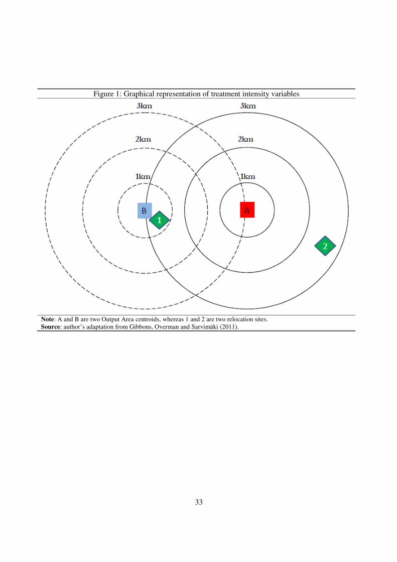
33
Figure 1: Graphical representation of treatment intensity variables
Note: A and B are two Output Area centroids, whereas 1 and 2 are two relocation sites.
Source: author’s adaptation from Gibbons, Overman and Sarvimäki (2011).
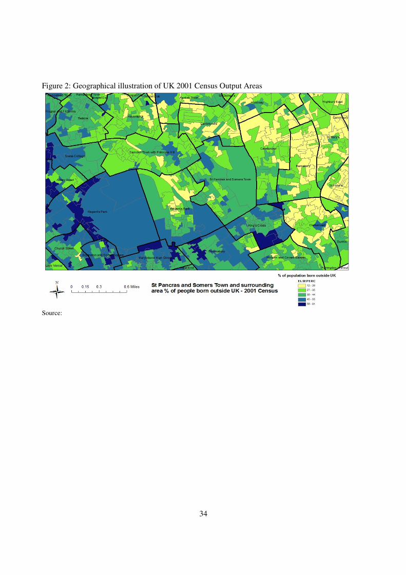
34
Figure 2: Geographical illustration of UK 2001 Census Output Areas
Source:
35
Figure 3: The impact of the Lyons Review on private sector employment, Log changes 2003-2008
Full specification including 50km treatment intensities and 2001 Census controls
Note: The dependent variable is expressed as the Log (2003-2008) changes in total private sector employment.
Source: BSD establishment data aggregated up to the 2001 Output Area level (2003-2008); 64 OA control variables
retrieved from the UK 2001 Census (See Appendix B for details).
-.04
-.02
0.0
2.0
4
Para
mete
r estim
ate
0 10 20 30 40 50Treatment Intensity
95%
Confidence inte
rval and
Total Private Employment with Controls
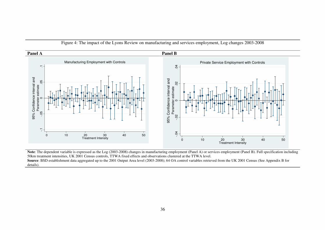
36
Figure 4: The impact of the Lyons Review on manufacturing and services employment, Log changes 2003-2008
Panel A Panel B
Note: The dependent variable is expressed as the Log (2003-2008) changes in manufacturing employment (Panel A) or services employment (Panel B). Full specification including
50km treatment intensities, UK 2001 Census controls, TTWA fixed effects and observations clustered at the TTWA level.
Source: BSD establishment data aggregated up to the 2001 Output Area level (2003-2008); 64 OA control variables retrieved from the UK 2001 Census (See Appendix B for
details).
-.1
-.05
0.0
5.1
Pa
ram
ete
r e
stim
ate
0 10 20 30 40 50Treatment Intensity
95%
Confidence inte
rval and
Manufacturing Employment with Controls
-.04
-.02
0.0
2.0
4P
ara
me
ter
estim
ate
0 10 20 30 40 50Treatment Intensity
95%
Co
nfid
en
ce in
terv
al a
nd
Private Service Employment with Controls

37
Table 1: Descriptive Statistics for Local Authorities chosen/not chosen as a relocation site
Variables LAs chosen LAs not chosen LAs in London and the South
East
Mean Standard
Deviation
Mean Standard
Deviation
Mean Standard
Deviation
Labour Market variables:
Share of public sector employment 0.239 0.062 0.201 0.068 0.178 0.060
Unemployment rate 4.9 1.7 4.1 1.4 4.8 2.2
Inactivity rate 0.222 0.050 0.198 0.050 0.204 0.060
Employment rate 0.739 0.058 0.769 0.056 0.758 0.072
Share of full-time workers 0.752 0.029 0.740 0.041 0.762 0.045
Share of part-time workers 0.248 0.029 0.260 0.041 0.237 0.045
Self-employment 0.114 0.038 0.134 0.050 0.150 0.040
Demographic variables:
Share of Whites 0.948 0.067 0.974 0.039 0.865 0.153
Skills: College degree and above 0.236 0.065 0.236 0.068 0.292 0.079
Skills: A-Levels and Equiv. 0.149 0.026 0.149 0.028 0.144 0.029
Skills: O-Levels and Equiv. 0.156 0.027 0.162 0.028 0.148 0.038
Skills: Apprenticeship 0.069 0.020 0.075 0.024 0.053 0.022
Skills: Foundation 0.153 0.029 0.153 0.036 0.137 0.042
Skills: Other 0.076 0.019 0.075 0.024 0.107 0.054
Skills: No Qual. 0.161 0.050 0.151 0.051 0.118 0.047
Political and Housing variables:
Share of Labour Votes 1983 Election 0.203 0.090 0.161 0.093 0.131 0.072
Share of Labour Votes 1997 Election 0.332 0.105 0.285 0.112 0.244 0.100
Share of Labour Votes 2005 Election 0.398 0.129 0.321 0.139 0.285 0.126
House prices in Land Registry data 126,364 42,060 145,625 46,047 227,206 75,216
Real mix-adjusted house prices index
composed of CML and Registry data
223.2 35.7 229.1 31.1 261.9 41.8
2004 Index of Multiple Deprivation:
Total number of English LAs 88 165 99
Number of Poor Areas (according to
the Index of Multiple Deprivation)
34 25 21
As % of all IMD areas 0.425 0.313 0.263
Note: All but the Index of Multiple Deprivation (IMD) figures are as of 2003. Education variables are expressed as the 2003 local
share of working age population (16-64 years old) with the relevant education qualification. The 2003 local unemployment rate refers
to the model-based unemployment rate derived by the ONS which combines unemployment information from the Annual Population
Survey and the number of beneficiaries of Jobseeker’s Allowance. English LAs are classified as poor areas according to the 2004
Index of Multiple Deprivation if they ranked among the 50 worst local authorities against any of the six local authority IMD indices.
Source: BIS Local Authority data (2003-2007); ABI Local Authority data (2003-2007); Local Area Labour Force Survey (1999-
2003); ONS Model-based Estimates of Unemployment (1999-2007); Land Registry data (2000-2010); 2004 Index of Multiple
Deprivation statistics. Shares of labour votes at the 1983, 1997 and 2005 elections as well as real mix-adjusted house prices index
have been kindly provided by Christian Hilber and Wouter Vermeulen. Because of missing data, two LAs are excluded: City of
London and Isles of Scilly.
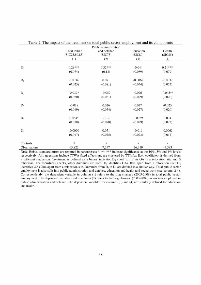
38
Table 2: The impact of the treatment on total public sector employment and its components
Total Public
(SIC75,80,85)
Public administration
and defence
(SIC75)
Education
(SIC80)
Health
(SIC85)
(1) (2) (3) (4)
D0 0.29*** 0.32*** -0.044 0.21***
(0.074) (0.12) (0.089) (0.079)
D1 0.0034 0.091 -0.0062 -0.0032
(0.023) (0.081) (0.034) (0.023)
D2 -0.037* -0.059 0.026 -0.045**
(0.020) (0.061) (0.029) (0.020)
D3 -0.018 0.026 0.027 -0.025
(0.019) (0.074) (0.027) (0.020)
D4 0.034* -0.12 0.0029 0.034
(0.018) (0.078) (0.029) (0.022)
D5 -0.0090 0.071 -0.016 -0.0065
(0.017) (0.075) (0.023) (0.017)
Controls √ √ √ √
Observations 65,822 7,257 26,319 43,383
Note: Robust standard errors are reported in parentheses; *, **, *** indicate significance at the 10%, 5% and 1% levels
respectively. All regressions include TTWA fixed effects and are clustered by TTWAs. Each coefficient is derived from
a different regression. Treatment is defined as a binary indicator D0 equal to1 if an OA is a relocation site and 0
otherwise. For robustness checks, other dummies are used: D1 identifies OAs 1km apart from a relocation site; D2
identifies OAs 2km apart from a relocation site. Dummies from D3 to D5 are defined in a similar way. Total public sector
employment is also split into public administration and defence, education and health and social work (see column 2-4).
Correspondently, the dependent variable in column (1) refers to the Log changes (2003-2008) in total public sector
employment. The dependent variable used in column (2) refers to the Log changes (2003-2008) in workers employed in
public administration and defence. The dependent variables for columns (3) and (4) are similarly defined for education
and health.

39
Table 3a: The Impact of the Lyons Review on private sector employment, Log 2003-2008
Employment Changes, treatment intensities measured as relocation dummies
Private Manuf Services Private Manuf Services
(1) (2) (3) (4) (5) (6)
0-1km dummy 0.028 -0.079* 0.031 0.036** -0.027 0.034*
(0.019) (0.046) (0.020) (0.018) (0.046) (0.019)
0-2km dummy -0.031*** -0.022 -0.027** -0.017 0.014 -0.017
(0.011) (0.035) (0.011) (0.011) (0.034) (0.011)
0-3km dummy -0.012 -0.014 -0.012 -0.006 -0.002 -0.008
(0.0097) (0.032) (0.010) (0.009) (0.034) (0.010)
0-4km dummy -0.011 -0.034 -0.0037 -0.008 -0.020 -0.001
(0.011) (0.027) (0.012) (0.010) (0.025) (0.011)
0-5km dummy 0.0072 -0.0076 -0.0025 0.022** 0.024 0.014
(0.011) (0.029) (0.012) (0.009) (0.026) (0.010)
Constant 0.061*** -0.12*** 0.091*** -0.220 -0.490 -0.100
(0.002) (0.004) (0.002) (0.160) (0.390) (0.180)
Controls No No No √ √ √
Observations 160,874 39,187 158,954 155,608 38,353 153,747
R-squared 0.004 0.010 0.004 0.008 0.017 0.008
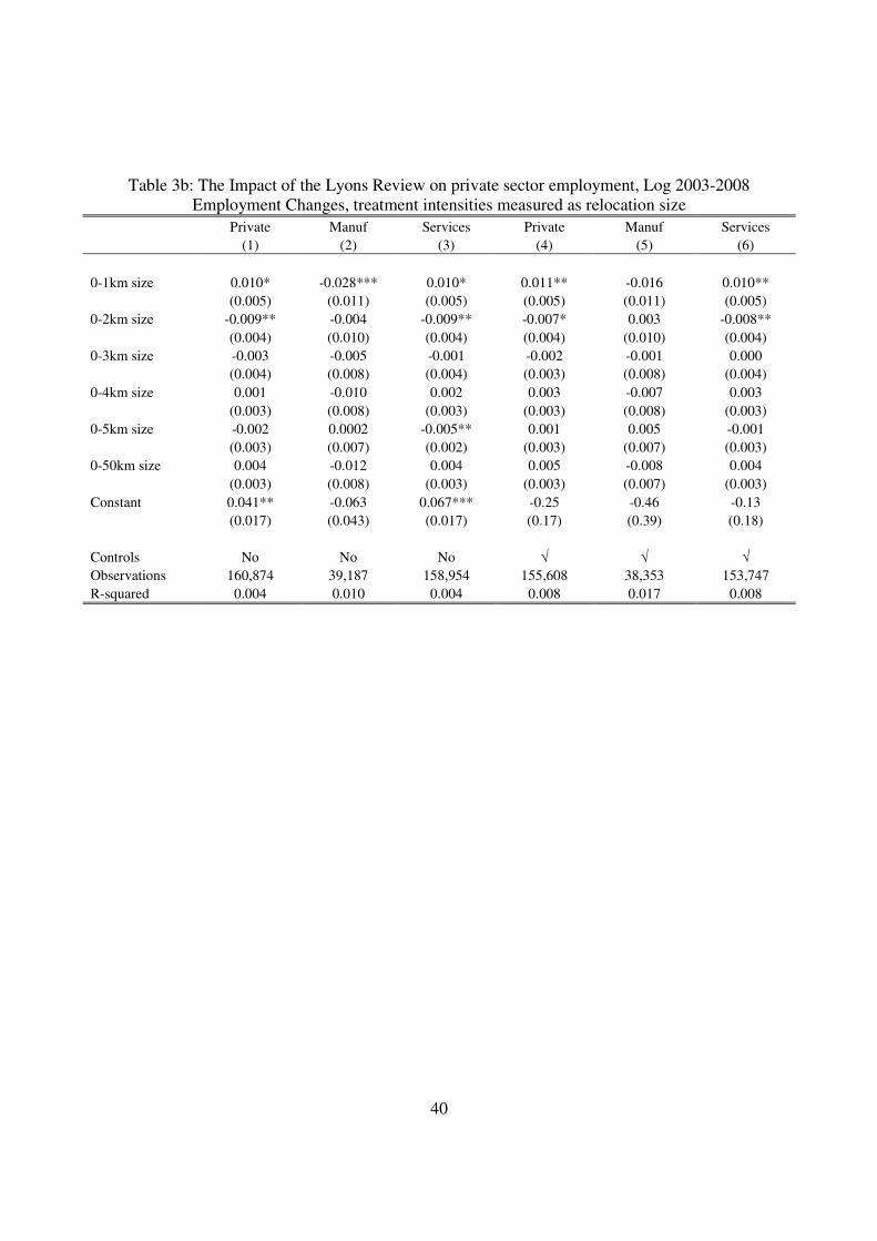
40
Table 3b: The Impact of the Lyons Review on private sector employment, Log 2003-2008
Employment Changes, treatment intensities measured as relocation size
Private Manuf Services Private Manuf Services
(1) (2) (3) (4) (5) (6)
0-1km size 0.010* -0.028*** 0.010* 0.011** -0.016 0.010**
(0.005) (0.011) (0.005) (0.005) (0.011) (0.005)
0-2km size -0.009** -0.004 -0.009** -0.007* 0.003 -0.008**
(0.004) (0.010) (0.004) (0.004) (0.010) (0.004)
0-3km size -0.003 -0.005 -0.001 -0.002 -0.001 0.000
(0.004) (0.008) (0.004) (0.003) (0.008) (0.004)
0-4km size 0.001 -0.010 0.002 0.003 -0.007 0.003
(0.003) (0.008) (0.003) (0.003) (0.008) (0.003)
0-5km size -0.002 0.0002 -0.005** 0.001 0.005 -0.001
(0.003) (0.007) (0.002) (0.003) (0.007) (0.003)
0-50km size 0.004 -0.012 0.004 0.005 -0.008 0.004
(0.003) (0.008) (0.003) (0.003) (0.007) (0.003)
Constant 0.041** -0.063 0.067*** -0.25 -0.46 -0.13
(0.017) (0.043) (0.017) (0.17) (0.39) (0.18)
Controls No No No √ √ √
Observations 160,874 39,187 158,954 155,608 38,353 153,747
R-squared 0.004 0.010 0.004 0.008 0.017 0.008
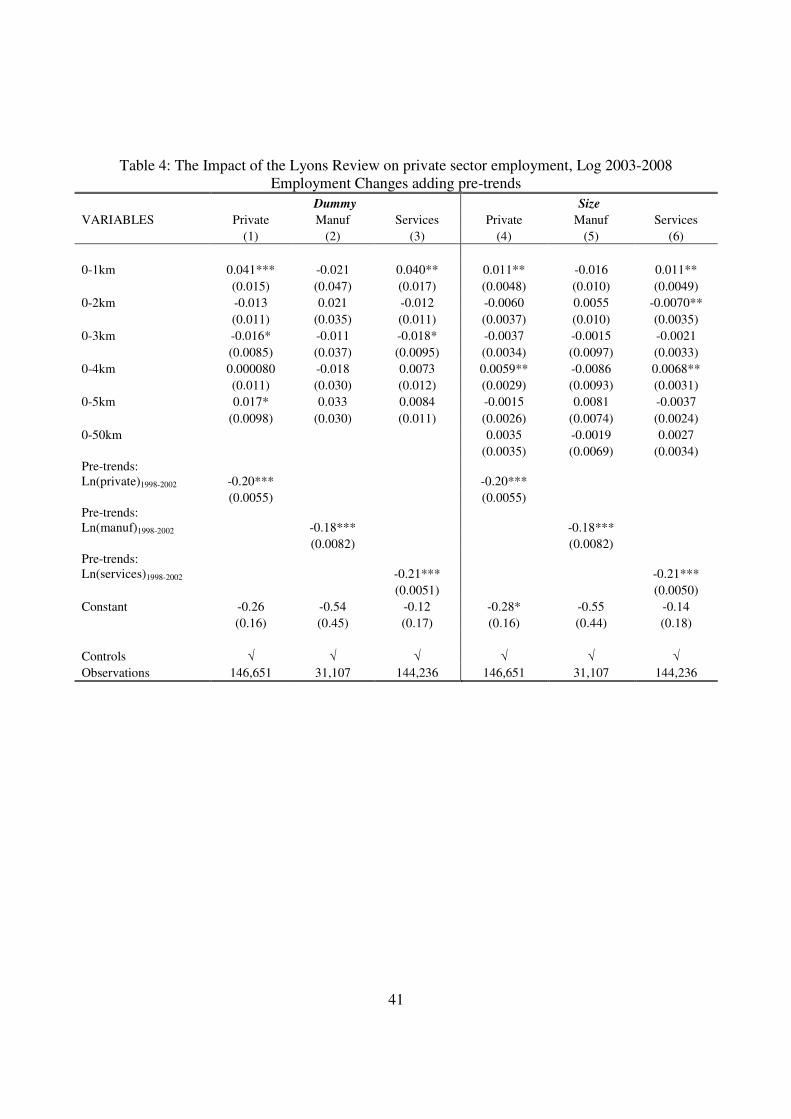
41
Table 4: The Impact of the Lyons Review on private sector employment, Log 2003-2008
Employment Changes adding pre-trends
Dummy Size
VARIABLES Private Manuf Services Private Manuf Services
(1) (2) (3) (4) (5) (6)
0-1km 0.041*** -0.021 0.040** 0.011** -0.016 0.011**
(0.015) (0.047) (0.017) (0.0048) (0.010) (0.0049)
0-2km -0.013 0.021 -0.012 -0.0060 0.0055 -0.0070**
(0.011) (0.035) (0.011) (0.0037) (0.010) (0.0035)
0-3km -0.016* -0.011 -0.018* -0.0037 -0.0015 -0.0021
(0.0085) (0.037) (0.0095) (0.0034) (0.0097) (0.0033)
0-4km 0.000080 -0.018 0.0073 0.0059** -0.0086 0.0068**
(0.011) (0.030) (0.012) (0.0029) (0.0093) (0.0031)
0-5km 0.017* 0.033 0.0084 -0.0015 0.0081 -0.0037
(0.0098) (0.030) (0.011) (0.0026) (0.0074) (0.0024)
0-50km 0.0035 -0.0019 0.0027
(0.0035) (0.0069) (0.0034)
Pre-trends:
Ln(private)1998-2002 -0.20*** -0.20***
(0.0055) (0.0055)
Pre-trends:
Ln(manuf)1998-2002 -0.18*** -0.18***
(0.0082) (0.0082)
Pre-trends:
Ln(services)1998-2002 -0.21*** -0.21***
(0.0051) (0.0050)
Constant -0.26 -0.54 -0.12 -0.28* -0.55 -0.14
(0.16) (0.45) (0.17) (0.16) (0.44) (0.18)
Controls √ √ √ √ √ √
Observations 146,651 31,107 144,236 146,651 31,107 144,236
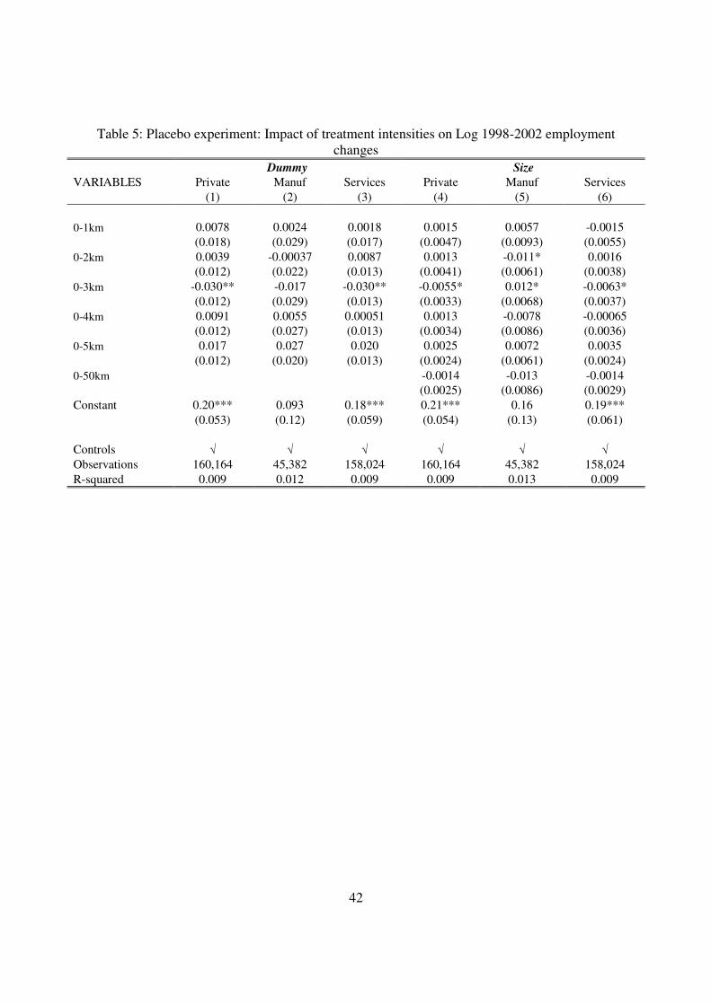
42
Table 5: Placebo experiment: Impact of treatment intensities on Log 1998-2002 employment
changes
Dummy Size
VARIABLES Private Manuf Services Private Manuf Services
(1) (2) (3) (4) (5) (6)
0-1km 0.0078 0.0024 0.0018 0.0015 0.0057 -0.0015
(0.018) (0.029) (0.017) (0.0047) (0.0093) (0.0055)
0-2km 0.0039 -0.00037 0.0087 0.0013 -0.011* 0.0016
(0.012) (0.022) (0.013) (0.0041) (0.0061) (0.0038)
0-3km -0.030** -0.017 -0.030** -0.0055* 0.012* -0.0063*
(0.012) (0.029) (0.013) (0.0033) (0.0068) (0.0037)
0-4km 0.0091 0.0055 0.00051 0.0013 -0.0078 -0.00065
(0.012) (0.027) (0.013) (0.0034) (0.0086) (0.0036)
0-5km 0.017 0.027 0.020 0.0025 0.0072 0.0035
(0.012) (0.020) (0.013) (0.0024) (0.0061) (0.0024)
0-50km -0.0014 -0.013 -0.0014
(0.0025) (0.0086) (0.0029)
Constant 0.20*** 0.093 0.18*** 0.21*** 0.16 0.19***
(0.053) (0.12) (0.059) (0.054) (0.13) (0.061)
Controls √ √ √ √ √ √
Observations 160,164 45,382 158,024 160,164 45,382 158,024
R-squared 0.009 0.012 0.009 0.009 0.013 0.009

43
Table 6: Test for causality: Impact of treatment intensities on Log employment changes before and
after the implementation of the Lyons Review
Private Manuf Services
Dep.Var. (1) (2) (3)
Log 1998-1999 emp -0.00070 0.0032 -0.0012
(0.0028) (0.0050) (0.0030)
Observations 165,671 55,207 163,714
Log 1999-2000 emp -0.0012 -0.00041 -0.0021
(0.0027) (0.0058) (0.0029)
Observations 165,113 53,708 163,188
Log 2000-2001 emp 0.0013 0.0061 0.000027
(0.0027) (0.0049) (0.0028)
Observations 165,498 54,178 163,617
Log 2001-2002 0.0032 -0.0024 0.0021
(0.0034) (0.0056) (0.0032)
Observations 165,498 54,178 163,617
Log 2002-2003 emp -0.0011 -0.0079 0.000034
(0.0032) (0.0049) (0.0033)
Observations 159,275 58,561 157,511
Log 2003-2008 emp 0.011** -0.016 0.010**
(0.0050) (0.011) (0.0051)
Observations 155,608 38,353 153,747
Log 2008-2009 emp -0.0021 0.00018 -0.0025
(0.0024) (0.0058) (0.0023)
Observations 164,710 49,235 163,359
Note: Robust standard errors are reported in parentheses; *, **, *** indicate significance at the 10%, 5% and 1% levels
respectively. All regressions include area controls (1991 or 2001 UK Census), TTWA fixed effects and are clustered at
the TTWA level. Each row refers to a different set of regressions using the dependent variable indicated in the far-left
column.

44
Table 7: The relative importance of yearly relocations, Log 2003-2008 employment changes
Private Manuf Services
(1) (2) (3)
0-1km 2003-2004 0.024** -0.015 0.019**
(0.0093) (0.020) (0.0094)
0-1km 2005 -0.0021 -0.0043 -0.0063
(0.0082) (0.026) (0.0082)
0-1km 2006 -0.013* -0.012 -0.014
(0.0076) (0.020) (0.0085)
0-1km 2007 0.019* -0.0077 0.023**
(0.010) (0.025) (0.011)
0-2km 2003-2004 -0.021*** 0.00043 -0.020***
(0.0057) (0.012) (0.0061)
0-2km 2005 0.013* -0.0015 0.0099
(0.0077) (0.013) (0.0075)
0-2km 2006 -0.0044 0.0066 -0.0028
(0.0064) (0.014) (0.0061)
0-2km 2007 -0.00082 -0.0071 -0.00060
(0.0065) (0.017) (0.0063)
0-3km 2003-2004 0.0017 -0.0029 0.0034
(0.0058) (0.011) (0.0057)
0-3km 2005 0.0025 0.020 0.0018
(0.0061) (0.014) (0.0058)
0-3km 2006 -0.013*** -0.031** -0.011**
(0.0050) (0.012) (0.0050)
0-3km 2007 0.0059* 0.016 0.0068*
(0.0032) (0.014) (0.0036)
0-4km 2003-2004 0.0054 0.012 0.0037
(0.0052) (0.013) (0.0052)
0-4km 2005 -0.0033 -0.019 -0.0020
(0.0058) (0.018) (0.0053)
0-4km 2006 -0.0030 0.011 -0.0029
(0.0053) (0.013) (0.0051)
0-4km 2007 0.0061 -0.0089 0.0071*
(0.0041) (0.018) (0.0039)
0-5km 2003-2004 0.0011 -0.018* 0.0020
(0.0041) (0.010) (0.0038)
0-5km 2005 -0.0031 0.0099 -0.0034
(0.0045) (0.011) (0.0044)
0-5km 2006 0.0064 0.00012 0.0053
(0.0044) (0.011) (0.0040)
0-5km 2007 -0.0032 0.0084 -0.0055
(0.0045) (0.012) (0.0043)
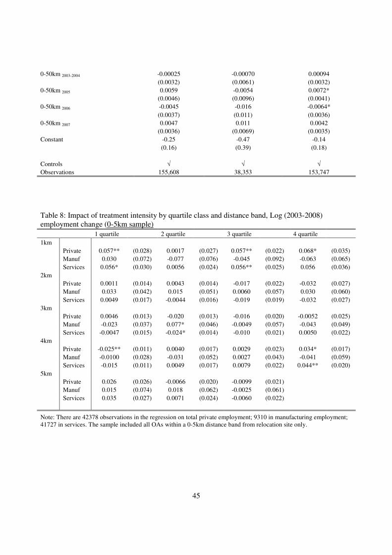
45
0-50km 2003-2004 -0.00025 -0.00070 0.00094
(0.0032) (0.0061) (0.0032)
0-50km 2005 0.0059 -0.0054 0.0072*
(0.0046) (0.0096) (0.0041)
0-50km 2006 -0.0045 -0.016 -0.0064*
(0.0037) (0.011) (0.0036)
0-50km 2007 0.0047 0.011 0.0042
(0.0036) (0.0069) (0.0035)
Constant -0.25 -0.47 -0.14
(0.16) (0.39) (0.18)
Controls √ √ √
Observations 155,608 38,353 153,747
Table 8: Impact of treatment intensity by quartile class and distance band, Log (2003-2008)
employment change (0-5km sample)
1 quartile 2 quartile 3 quartile 4 quartile
1km
Private 0.057** (0.028) 0.0017 (0.027) 0.057** (0.022) 0.068* (0.035)
Manuf 0.030 (0.072) -0.077 (0.076) -0.045 (0.092) -0.063 (0.065)
Services 0.056* (0.030) 0.0056 (0.024) 0.056** (0.025) 0.056 (0.036)
2km
Private 0.0011 (0.014) 0.0043 (0.014) -0.017 (0.022) -0.032 (0.027)
Manuf 0.033 (0.042) 0.015 (0.051) 0.0060 (0.057) 0.030 (0.060)
Services 0.0049 (0.017) -0.0044 (0.016) -0.019 (0.019) -0.032 (0.027)
3km
Private 0.0046 (0.013) -0.020 (0.013) -0.016 (0.020) -0.0052 (0.025)
Manuf -0.023 (0.037) 0.077* (0.046) -0.0049 (0.057) -0.043 (0.049)
Services -0.0047 (0.015) -0.024* (0.014) -0.010 (0.021) 0.0050 (0.022)
4km
Private -0.025** (0.011) 0.0040 (0.017) 0.0029 (0.023) 0.034* (0.017)
Manuf -0.0100 (0.028) -0.031 (0.052) 0.0027 (0.043) -0.041 (0.059)
Services -0.015 (0.011) 0.0049 (0.017) 0.0079 (0.022) 0.044** (0.020)
5km
Private 0.026 (0.026) -0.0066 (0.020) -0.0099 (0.021)
Manuf 0.015 (0.074) 0.018 (0.062) -0.0025 (0.061)
Services 0.035 (0.027) 0.0071 (0.024) -0.0060 (0.022)
Note: There are 42378 observations in the regression on total private employment; 9310 in manufacturing employment;
41727 in services. The sample included all OAs within a 0-5km distance band from relocation site only.
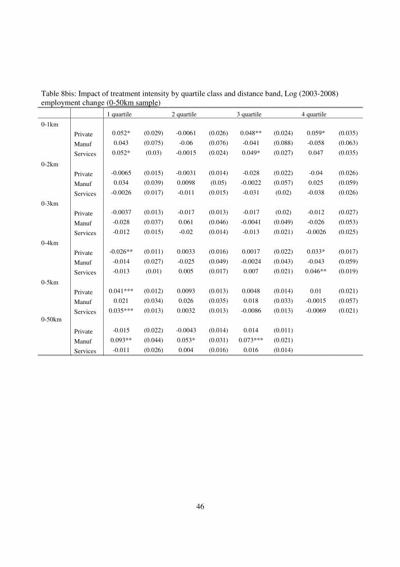
46
Table 8bis: Impact of treatment intensity by quartile class and distance band, Log (2003-2008)
employment change (0-50km sample) 1 quartile 2 quartile 3 quartile 4 quartile
0-1km
Private 0.052* (0.029) -0.0061 (0.026) 0.048** (0.024) 0.059* (0.035)
Manuf 0.043 (0.075) -0.06 (0.076) -0.041 (0.088) -0.058 (0.063)
Services 0.052* (0.03) -0.0015 (0.024) 0.049* (0.027) 0.047 (0.035)
0-2km
Private -0.0065 (0.015) -0.0031 (0.014) -0.028 (0.022) -0.04 (0.026)
Manuf 0.034 (0.039) 0.0098 (0.05) -0.0022 (0.057) 0.025 (0.059)
Services -0.0026 (0.017) -0.011 (0.015) -0.031 (0.02) -0.038 (0.026)
0-3km
Private -0.0037 (0.013) -0.017 (0.013) -0.017 (0.02) -0.012 (0.027)
Manuf -0.028 (0.037) 0.061 (0.046) -0.0041 (0.049) -0.026 (0.053)
Services -0.012 (0.015) -0.02 (0.014) -0.013 (0.021) -0.0026 (0.025)
0-4km
Private -0.026** (0.011) 0.0033 (0.016) 0.0017 (0.022) 0.033* (0.017)
Manuf -0.014 (0.027) -0.025 (0.049) -0.0024 (0.043) -0.043 (0.059)
Services -0.013 (0.01) 0.005 (0.017) 0.007 (0.021) 0.046** (0.019)
0-5km
Private 0.041*** (0.012) 0.0093 (0.013) 0.0048 (0.014) 0.01 (0.021)
Manuf 0.021 (0.034) 0.026 (0.035) 0.018 (0.033) -0.0015 (0.057)
Services 0.035*** (0.013) 0.0032 (0.013) -0.0086 (0.013) -0.0069 (0.021)
0-50km Private -0.015 (0.022) -0.0043 (0.014) 0.014 (0.011)
Manuf 0.093** (0.044) 0.053* (0.031) 0.073*** (0.021)
Services -0.011 (0.026) 0.004 (0.016) 0.016 (0.014)
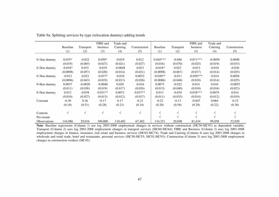
47
Table 9a: Splitting services by type (relocation dummy) adding trends
Baseline Transport
FIRE and
business
Trade and
Catering Construction Baseline Transport
FIRE and
business
Trade and
Catering Construction
(1) (2) (3) (4) (5) (1) (2) (3) (4) (5)
0-1km dummy 0.035* -0.022 0.050* -0.019 0.012 0.045*** -0.046 0.071*** -0.0050 0.0040
(0.019) (0.065) (0.027) (0.021) (0.027) (0.016) (0.070) (0.025) (0.019) (0.033)
0-2km dummy -0.018* 0.015 -0.019 -0.0048 -0.031 -0.018* 0.023 -0.013 -0.010 -0.030
(0.0098) (0.057) (0.020) (0.014) (0.021) (0.0098) (0.067) (0.017) (0.014) (0.025)
0-3km dummy -0.012 -0.021 -0.037* -0.010 0.0032 -0.020** -0.011 -0.058*** -0.014 0.0056
(0.0096) (0.043) (0.019) (0.013) (0.026) (0.0088) (0.048) (0.018) (0.014) (0.025)
0-4km dummy 0.0037 -0.0020 -0.0040 0.020 -0.016 0.0073 -0.022 0.014 0.016 -0.0055
(0.011) (0.038) (0.019) (0.017) (0.024) (0.013) (0.040) (0.018) (0.016) (0.023)
0-5km dummy 0.012 -0.038 0.031** 0.0071 0.037** 0.013 -0.034 0.038*** 0.0079 0.014
(0.010) (0.027) (0.013) (0.012) (0.017) (0.011) (0.035) (0.014) (0.012) (0.019)
Constant -0.30 0.36 -0.17 0.17 -0.21 -0.22 -0.13 -0.047 0.064 -0.32
(0.19) (0.51) (0.28) (0.21) (0.34) (0.20) (0.58) (0.29) (0.22) (0.38)
Controls √ √ √ √ √ √ √ √ √ √ Pre-trends √ √ √ √ √ Observations 144,986 29,016 100,800 110,402 67,482 134,351 20,698 81,634 99,858 52,020
Note: Baseline regressions (Column 1) use log 2003-2008 employment changes in services without construction (SIC50-SIC93) as dependent variable;
Transport (Column 2) uses log 2003-2008 employment changes in transport services (SIC60-SIC64); FIRE and Business (Column 3) uses log 2003-2008
employment changes in finance, insurance, real estate and business services (SIC65-SIC74); Trade and Catering (Column 4) uses log 2003-2008 changes in
wholesale and retail trade, hotel and restaurants, personal services (SIC50-SIC55; SIC92-SIC93); Construction (Column 5) uses log 2003-2008 employment
changes in construction workers (SIC45).
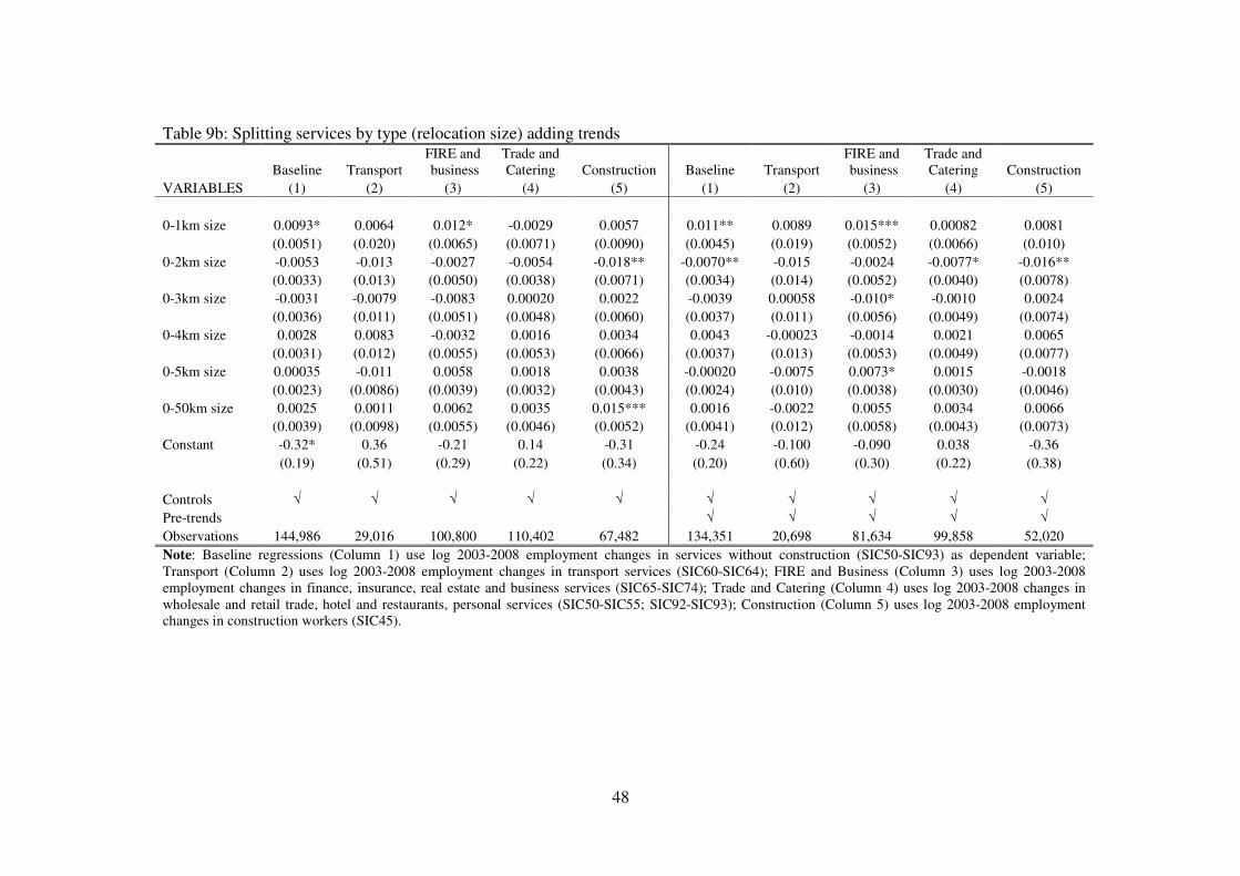
48
Table 9b: Splitting services by type (relocation size) adding trends
Baseline Transport
FIRE and
business
Trade and
Catering Construction Baseline Transport
FIRE and
business
Trade and
Catering Construction
VARIABLES (1) (2) (3) (4) (5) (1) (2) (3) (4) (5)
0-1km size 0.0093* 0.0064 0.012* -0.0029 0.0057 0.011** 0.0089 0.015*** 0.00082 0.0081
(0.0051) (0.020) (0.0065) (0.0071) (0.0090) (0.0045) (0.019) (0.0052) (0.0066) (0.010)
0-2km size -0.0053 -0.013 -0.0027 -0.0054 -0.018** -0.0070** -0.015 -0.0024 -0.0077* -0.016**
(0.0033) (0.013) (0.0050) (0.0038) (0.0071) (0.0034) (0.014) (0.0052) (0.0040) (0.0078)
0-3km size -0.0031 -0.0079 -0.0083 0.00020 0.0022 -0.0039 0.00058 -0.010* -0.0010 0.0024
(0.0036) (0.011) (0.0051) (0.0048) (0.0060) (0.0037) (0.011) (0.0056) (0.0049) (0.0074)
0-4km size 0.0028 0.0083 -0.0032 0.0016 0.0034 0.0043 -0.00023 -0.0014 0.0021 0.0065
(0.0031) (0.012) (0.0055) (0.0053) (0.0066) (0.0037) (0.013) (0.0053) (0.0049) (0.0077)
0-5km size 0.00035 -0.011 0.0058 0.0018 0.0038 -0.00020 -0.0075 0.0073* 0.0015 -0.0018
(0.0023) (0.0086) (0.0039) (0.0032) (0.0043) (0.0024) (0.010) (0.0038) (0.0030) (0.0046)
0-50km size 0.0025 0.0011 0.0062 0.0035 0.015*** 0.0016 -0.0022 0.0055 0.0034 0.0066
(0.0039) (0.0098) (0.0055) (0.0046) (0.0052) (0.0041) (0.012) (0.0058) (0.0043) (0.0073)
Constant -0.32* 0.36 -0.21 0.14 -0.31 -0.24 -0.100 -0.090 0.038 -0.36
(0.19) (0.51) (0.29) (0.22) (0.34) (0.20) (0.60) (0.30) (0.22) (0.38)
Controls √ √ √ √ √ √ √ √ √ √
Pre-trends √ √ √ √ √
Observations 144,986 29,016 100,800 110,402 67,482 134,351 20,698 81,634 99,858 52,020
Note: Baseline regressions (Column 1) use log 2003-2008 employment changes in services without construction (SIC50-SIC93) as dependent variable;
Transport (Column 2) uses log 2003-2008 employment changes in transport services (SIC60-SIC64); FIRE and Business (Column 3) uses log 2003-2008
employment changes in finance, insurance, real estate and business services (SIC65-SIC74); Trade and Catering (Column 4) uses log 2003-2008 changes in
wholesale and retail trade, hotel and restaurants, personal services (SIC50-SIC55; SIC92-SIC93); Construction (Column 5) uses log 2003-2008 employment
changes in construction workers (SIC45).
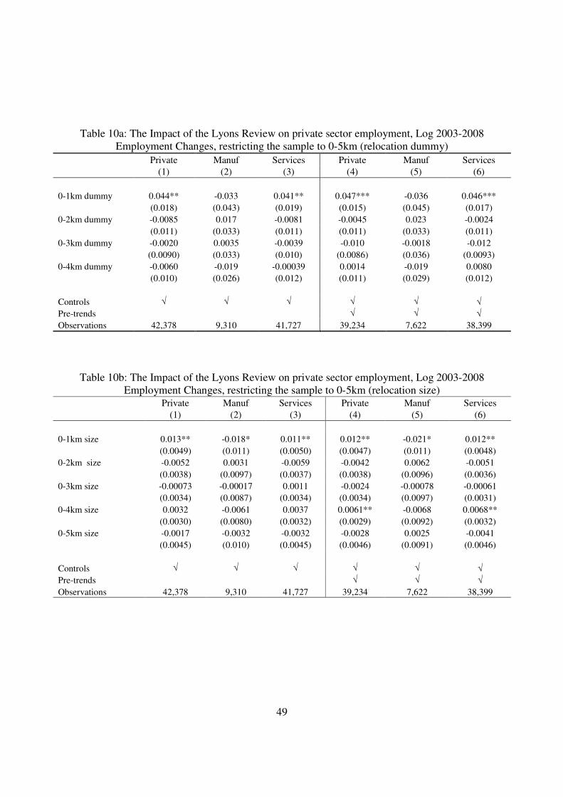
49
Table 10a: The Impact of the Lyons Review on private sector employment, Log 2003-2008
Employment Changes, restricting the sample to 0-5km (relocation dummy)
Private Manuf Services Private Manuf Services
(1) (2) (3) (4) (5) (6)
0-1km dummy 0.044** -0.033 0.041** 0.047*** -0.036 0.046***
(0.018) (0.043) (0.019) (0.015) (0.045) (0.017)
0-2km dummy -0.0085 0.017 -0.0081 -0.0045 0.023 -0.0024
(0.011) (0.033) (0.011) (0.011) (0.033) (0.011)
0-3km dummy -0.0020 0.0035 -0.0039 -0.010 -0.0018 -0.012
(0.0090) (0.033) (0.010) (0.0086) (0.036) (0.0093)
0-4km dummy -0.0060 -0.019 -0.00039 0.0014 -0.019 0.0080
(0.010) (0.026) (0.012) (0.011) (0.029) (0.012)
Controls √ √ √ √ √ √
Pre-trends √ √ √
Observations 42,378 9,310 41,727 39,234 7,622 38,399
Table 10b: The Impact of the Lyons Review on private sector employment, Log 2003-2008
Employment Changes, restricting the sample to 0-5km (relocation size)
Private Manuf Services Private Manuf Services
(1) (2) (3) (4) (5) (6)
0-1km size 0.013** -0.018* 0.011** 0.012** -0.021* 0.012**
(0.0049) (0.011) (0.0050) (0.0047) (0.011) (0.0048)
0-2km size -0.0052 0.0031 -0.0059 -0.0042 0.0062 -0.0051
(0.0038) (0.0097) (0.0037) (0.0038) (0.0096) (0.0036)
0-3km size -0.00073 -0.00017 0.0011 -0.0024 -0.00078 -0.00061
(0.0034) (0.0087) (0.0034) (0.0034) (0.0097) (0.0031)
0-4km size 0.0032 -0.0061 0.0037 0.0061** -0.0068 0.0068**
(0.0030) (0.0080) (0.0032) (0.0029) (0.0092) (0.0032)
0-5km size -0.0017 -0.0032 -0.0032 -0.0028 0.0025 -0.0041
(0.0045) (0.010) (0.0045) (0.0046) (0.0091) (0.0046)
Controls √ √ √ √ √ √
Pre-trends √ √ √
Observations 42,378 9,310 41,727 39,234 7,622 38,399
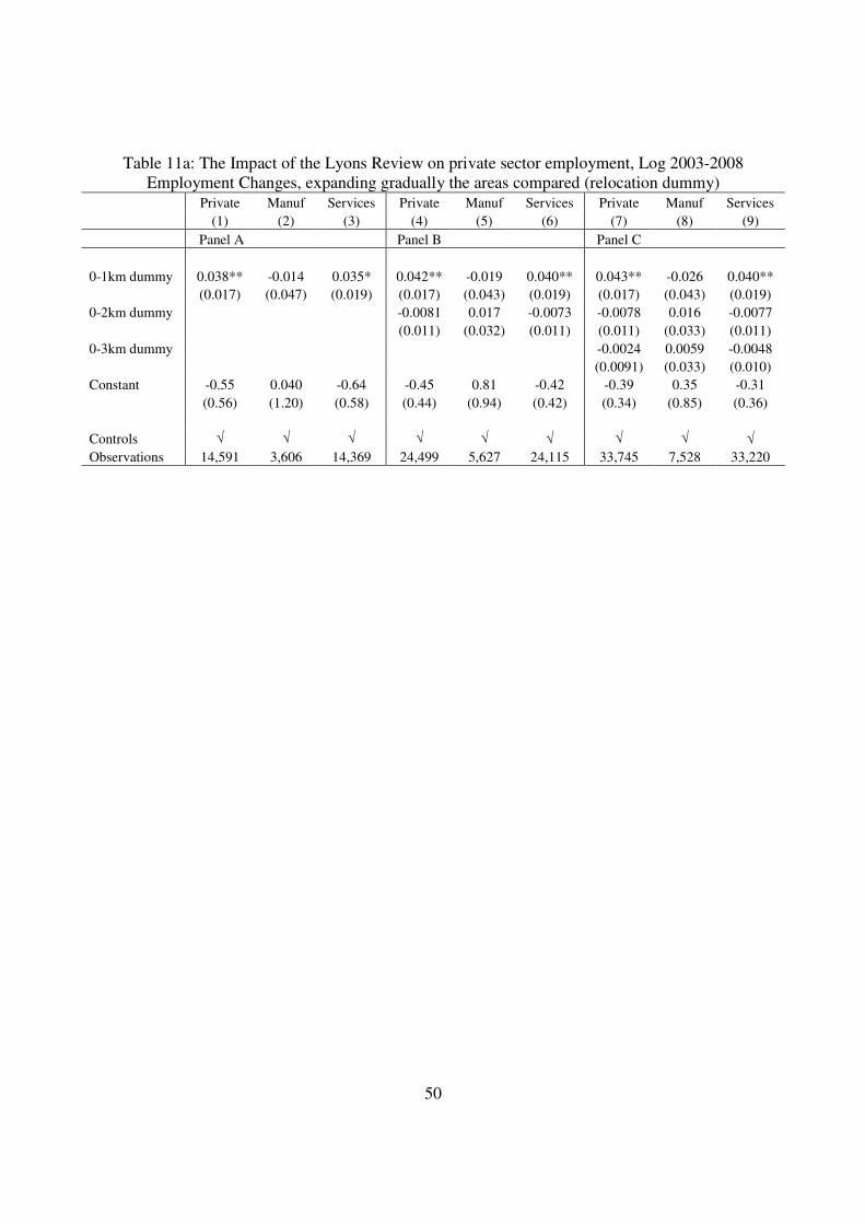
50
Table 11a: The Impact of the Lyons Review on private sector employment, Log 2003-2008
Employment Changes, expanding gradually the areas compared (relocation dummy)
Private Manuf Services Private Manuf Services Private Manuf Services
(1) (2) (3) (4) (5) (6) (7) (8) (9)
Panel A Panel B Panel C
0-1km dummy 0.038** -0.014 0.035* 0.042** -0.019 0.040** 0.043** -0.026 0.040**
(0.017) (0.047) (0.019) (0.017) (0.043) (0.019) (0.017) (0.043) (0.019)
0-2km dummy -0.0081 0.017 -0.0073 -0.0078 0.016 -0.0077
(0.011) (0.032) (0.011) (0.011) (0.033) (0.011)
0-3km dummy -0.0024 0.0059 -0.0048
(0.0091) (0.033) (0.010)
Constant -0.55 0.040 -0.64 -0.45 0.81 -0.42 -0.39 0.35 -0.31
(0.56) (1.20) (0.58) (0.44) (0.94) (0.42) (0.34) (0.85) (0.36)
Controls √ √ √ √ √ √ √ √ √
Observations 14,591 3,606 14,369 24,499 5,627 24,115 33,745 7,528 33,220
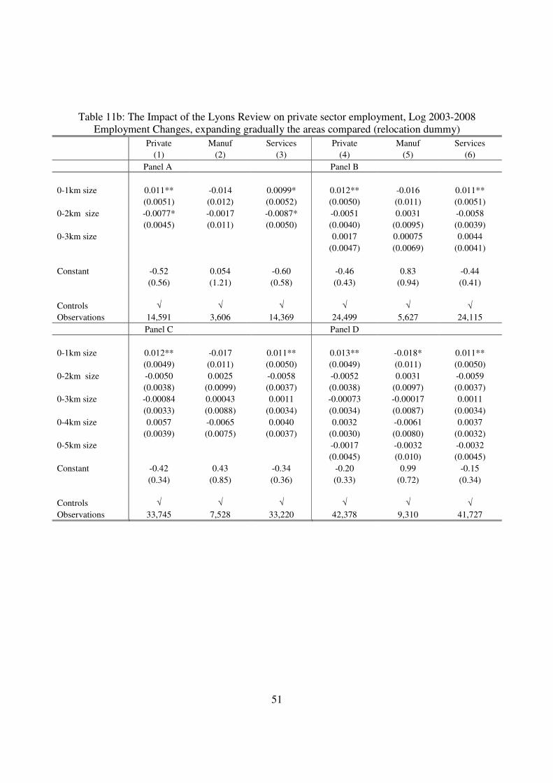
51
Table 11b: The Impact of the Lyons Review on private sector employment, Log 2003-2008
Employment Changes, expanding gradually the areas compared (relocation dummy)
Private Manuf Services Private Manuf Services
(1) (2) (3) (4) (5) (6)
Panel A Panel B
0-1km size 0.011** -0.014 0.0099* 0.012** -0.016 0.011**
(0.0051) (0.012) (0.0052) (0.0050) (0.011) (0.0051)
0-2km size -0.0077* -0.0017 -0.0087* -0.0051 0.0031 -0.0058
(0.0045) (0.011) (0.0050) (0.0040) (0.0095) (0.0039)
0-3km size 0.0017 0.00075 0.0044
(0.0047) (0.0069) (0.0041)
Constant -0.52 0.054 -0.60 -0.46 0.83 -0.44
(0.56) (1.21) (0.58) (0.43) (0.94) (0.41)
Controls √ √ √ √ √ √
Observations 14,591 3,606 14,369 24,499 5,627 24,115
Panel C Panel D
0-1km size 0.012** -0.017 0.011** 0.013** -0.018* 0.011**
(0.0049) (0.011) (0.0050) (0.0049) (0.011) (0.0050)
0-2km size -0.0050 0.0025 -0.0058 -0.0052 0.0031 -0.0059
(0.0038) (0.0099) (0.0037) (0.0038) (0.0097) (0.0037)
0-3km size -0.00084 0.00043 0.0011 -0.00073 -0.00017 0.0011
(0.0033) (0.0088) (0.0034) (0.0034) (0.0087) (0.0034)
0-4km size 0.0057 -0.0065 0.0040 0.0032 -0.0061 0.0037
(0.0039) (0.0075) (0.0037) (0.0030) (0.0080) (0.0032)
0-5km size -0.0017 -0.0032 -0.0032
(0.0045) (0.010) (0.0045)
Constant -0.42 0.43 -0.34 -0.20 0.99 -0.15
(0.34) (0.85) (0.36) (0.33) (0.72) (0.34)
Controls √ √ √ √ √ √
Observations 33,745 7,528 33,220 42,378 9,310 41,727

52
Appendix A
The Business Structure Database
The second database I use is the Business Structure Database (BSD), which provides an
annual snapshot (taken in April at the closing of the fiscal year) of the Inter-Departmental Business
Register (IDBR). The IDBR consists of administrative data collected for revenues and taxation
purposes and is constantly updated. Any business liable for value-added taxation (VAT) and/or with
at least one employee registered for tax collection will appear on the IDBR. For the year 2012, the
VAT threshold for registration was a turnover of taxable goods and services of £77,000, thus
suggesting that the BSD might not sample very small-businesses. Nevertheless, the ONS estimated
that for 2004 the businesses listed on the IDBR accounted for approximately 99 per cent of
economic activity in the UK.
The BSD data is structured into enterprises and local units. An enterprise is the overall
business organisation, whereas the local unit can be thought of as a plant or establishment. In the
majority of cases (about 70 per cent), enterprises only have one local unit, while in the remaining 30
per cent of cases enterprises have multiple local units. I focus on data at the establishment or plant
level. The BSD data contains information on about 2.4 million business establishments per year over
the period 1997-2009 and includes information on each business’ date of birth, date of death,
postcode, sector of activity (up to 4-digit Standard Industry Classification (SIC) 2003 code) and total
employment. Using the postcode, I assign each local unit active in England, Wales and Scotland to a
Census 2001 Output Area – the unit of observation I have chosen to conduct the analysis.
The initial raw data includes approximately 3 million local units every year. However, I carry
out a series of checks and drop a number of units. In particular, I drop cases where I identify
establishments opening/closing in a specific year, disappearing/reappearing in a subsequent year
only to open/close again in a subsequent wave. Stated differently, we only count firms’ birth and
death once. In addition, I drop active units with zero employment (this figure includes the
owners/managers of the establishment, so it cannot be zero for an active unit) and postcodes that
include an anomalous number of units in the same 3-digit industry. The adjustment for anomalous
postcodes consists of three parts: When I observe two or more plants operating in the same 3-digit
industry, sharing the same postcode34 and that are under common ownership, I believe this being an
34
A UK postcode or postal unit usually corresponds to a limited number of addresses or a single large delivery point. It
is not necessarily a geographically accurate description of where a property is located, but it is a good approximation.

53
error in reporting and drop them. In a non-trivial number of cases, I also observe plants sharing the
same 3-digit industry and the same postcode. I believe this being another coding error and trim the
top 5% of those plants’ distribution. Finally, looking at the employment distribution by 3-digit
industry, I also trimmed the top 1%.
Finally, I focus on private businesses and exclude active units operating in one of the
following sectors: Public Administration and Defence; Education; Health and Social Work; Public
Utilities (Electricity, Gas and Water). I also exclude businesses operating in Agriculture; Hunting
and Forestry; Fishing; Private Households with Employees; and Extra-Territorial Organization and
Bodies.
We also use the National Statistics Postcode Directory (NSPD) which is a list of all the current and
terminated postcodes that have ever existed in the UK, together with geographical links or matches
for each postcode to a variety of different administrative, health, electoral and other geographies that
are, or have been, used within the UK.
The NSPD is a collection of over 29 million Royal Mail postal addresses and postcodes. I use the
NSPD for matching postcodes of government relocation to in order to match government relocation
data with business postcodes to Census Output Area (OA) and then construct our measure of
employment and number of businesses by aggregating the BSD data by OA.
For instance, a building which contains several flats or businesses but only one external door, will only have the external
door listed as a delivery point. This example also shows that UK postcodes are geographically accurate up to the level of
a front door in a particular street.

54
Table A.1: List of control variables retrieved from the UK 1991 and 2001 Census
All control variables are constructed at the 2001 Output Area (OAs) level.
pop_less25 Proportion of population aged 24 or younger
pop_25_44 Proportion of population aged 25 to 44
pop_45_64 Proportion of population aged 45 to 64
pop_65_74 Proportion of population aged 65 to 74
pop_over75 Proportion of population aged 75+"
noqual_wap Proportion of WAP without qualifications
qlev1_wap Proportion of WAP with qualification level 1
qlev2_wap Proportion of WAP with qualification level 2
qlev3_wap Proportion of WAP with qualification level 3
qlev4o5_wap Proportion of WAP with qualification level 4 o 5
qoth_wap Proportion of WAP with other qualifications
pop_male Proportion of male population
pop_female Proportion of female population
pop_density Population density
emp_xstud emp-to-pop ratio - excluding students
inact_xstud inact-to-pop ratio - excluding students
un_xstud un-to-pop ratio - excluding students
sh_stud share of students in the WAP(16-74)
sh_ret share of retired individuals in the WAP(16-74)
work_se_rate Proportion of self-employed workers
Work_ft_rate Proportion of full-time employees
work_pt_rate Proportion of part-time employees
comm_emp Proportion of employees that travel to work
home_emp Proportion of employees working from home
Agri_sh Proportion of total employment in agriculture, hunting and forestry
Fish_sh Proportion of total employment in fishing
Min_sh Proportion of total employment in mining
Elect_sh Proportion of total employment in electricity and water supply
Man_sh Proportion of total employment in manufacturing
Const_sh Proportion of total employment in construction
Who_sh Proportion of total employment in wholesale and retail
Hot_sh Proportion of total employment in hotels/catering
Trans_sh Proportion of total employment in transport/communication
Fin_sh Proportion of total employment in financial interm
Est_sh Proportion of total employment in real estate/renting
Pub_sh Proportion of total employment in public admin and defense
Ed_sh Proportion of total employment in education
Hea_sh Proportion of total employment in health and social
Other_sh Proportion of total employment in other industries
elem_so_sh Proportion employed in elementary occupations over total
proc_so_sh Proportion employed as process/plant and machine operatives over total

55
sale_so_sh Proportion employed in sales and customer service occupations over total
pers_so_sh Proportion employed in personal service over total
skl_so_sh Proportion employed in skilled occupations over total
admin_so_sh Proportion employed in administrative/secretarial occupations over total
apro_so_sh Proportion employed in technical occupations over total
pro_so_sh Proportion employed in professional occupations over total
mangr_so_sh Proportion employed as managers/senior officials over total
white_sh Proportion of all whites over population
nowhite_sh Proportion of all non-whites over population
lone_hous Proportion of lone parent households over total households
migr_pop Proportion of non-UK born over total population
hous_overcr Proportion of overcrowded households
hous_avsize Average household size
hous_nbrooms Average number of rooms per household
hous_noheat Proportion of households without heating
hous_wocars Proportion of households without a car
Hous_allrent Proportion of households living in rented houses
hous_own Proportion of households living in owned houses
hous_privrent Proportion of private renters on total renters
hous_council Proportion of social renters on total renters
pop_estab Share of total population living in communal establishments
travel_undergr Proportion of employees travelling to work by tube
travel_train Proportion of employees travelling to work by train
travel_bus Proportion of employees travelling to work by bus
travel_motocy Proportion of employees travelling to work by motorcycle
travel_car Proportion of employees travelling to work by car
travel_carpas Proportion of employees travelling to work by common car
travel_taxi Proportion of employees travelling to work by taxi
travel_bike Proportion of employees travelling to work by bike
travel_foot Proportion of employees walking
travel_oth Proportion of employees travelling to work by other means
av_commdist Average distance (km) travelled to fixed place of work
pub_trans People in employment who use public transport
Source: UK Census data 2001.
Recommended