Reliable Computation of Equilibrium States and Bifurcations in Nonlinear Dynamics
C. Ryan GwaltneyMark A. Stadtherr
University of Notre Dame Department of Chemical and Biomolecular Engineering
Notre Dame, Indiana, USA
PARA '04June 22, 2004
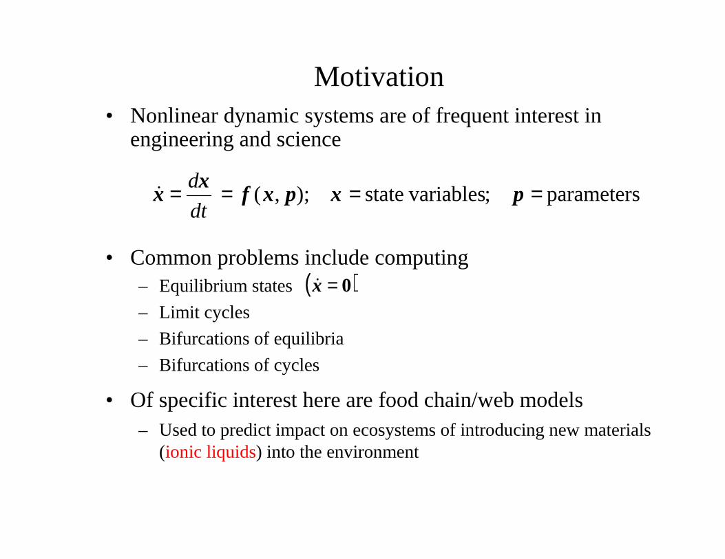
Motivation• Nonlinear dynamic systems are of frequent interest in
engineering and science
• Common problems include computing– Equilibrium states
– Limit cycles
– Bifurcations of equilibria
– Bifurcations of cycles
• Of specific interest here are food chain/web models– Used to predict impact on ecosystems of introducing new materials
(ionic liquids) into the environment
parameters ; variablesstate );,( ==== pxpxfx
xdt
d&
( )0=x&
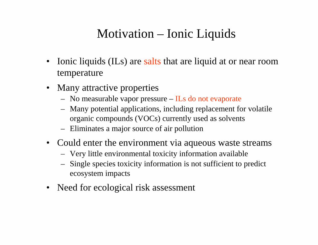
Motivation – Ionic Liquids
• Ionic liquids (ILs) are saltsthat are liquid at or near room temperature
• Many attractive properties– No measurable vapor pressure –ILs do not evaporate– Many potential applications, including replacement for volatile
organic compounds (VOCs) currently used as solvents– Eliminates a major source of air pollution
• Could enter the environment via aqueous waste streams– Very little environmental toxicity information available– Single species toxicity information is not sufficient to predict
ecosystem impacts
• Need for ecological risk assessment
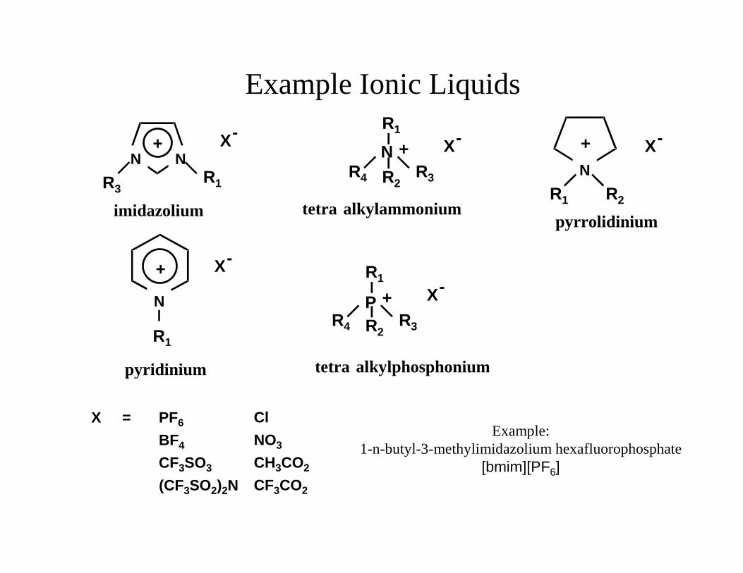
Example Ionic Liquids
Example:1-n-butyl-3-methylimidazolium hexafluorophosphate
[bmim][PF6]
N NR1R3
+ X-
imidazolium
N
R1
+ X-
pyridinium
tetra alkylammonium
N
R2R4 R3
R1
X-+
PR2
R4 R3
R1
X-+
tetra alkylphosphonium
N
+
R1 R2
pyrrolidinium
X-
X = PF6
BF4
CF3SO3
(CF3SO2)2N
Cl
NO3
CH3CO2
CF3CO2

Ecological Risk Assessment
• Aim to predict a variety of different consequences, e.g.,– Bioaccumulation and biomagnification– Contaminant transport and fate– Ecosystem toxicity effects
• Use a variety of different strategies and tools, e.g.,– Toxicology– Microbiology– Hydrology– Ecological Modeling
• Currently, food chain/web models are used to link single species toxicity tests to ecosystem toxicity effects– Results indicate that modeling can provide a conservative estimate
of allowable contaminate concentrations (e.g., Naito et al., 2002)
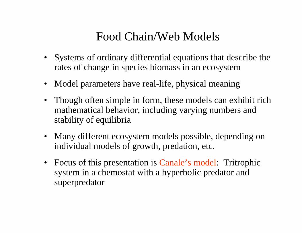
Food Chain/Web Models
• Systems of ordinary differential equations that describe the rates of change in species biomass in an ecosystem
• Model parameters have real-life, physical meaning
• Though often simple in form, these models can exhibit rich mathematical behavior, including varying numbers and stability of equilibria
• Many different ecosystem models possible, depending on individual models of growth, predation, etc.
• Focus of this presentation is Canale’s model: Tritrophic system in a chemostat with a hyperbolic predator and superpredator
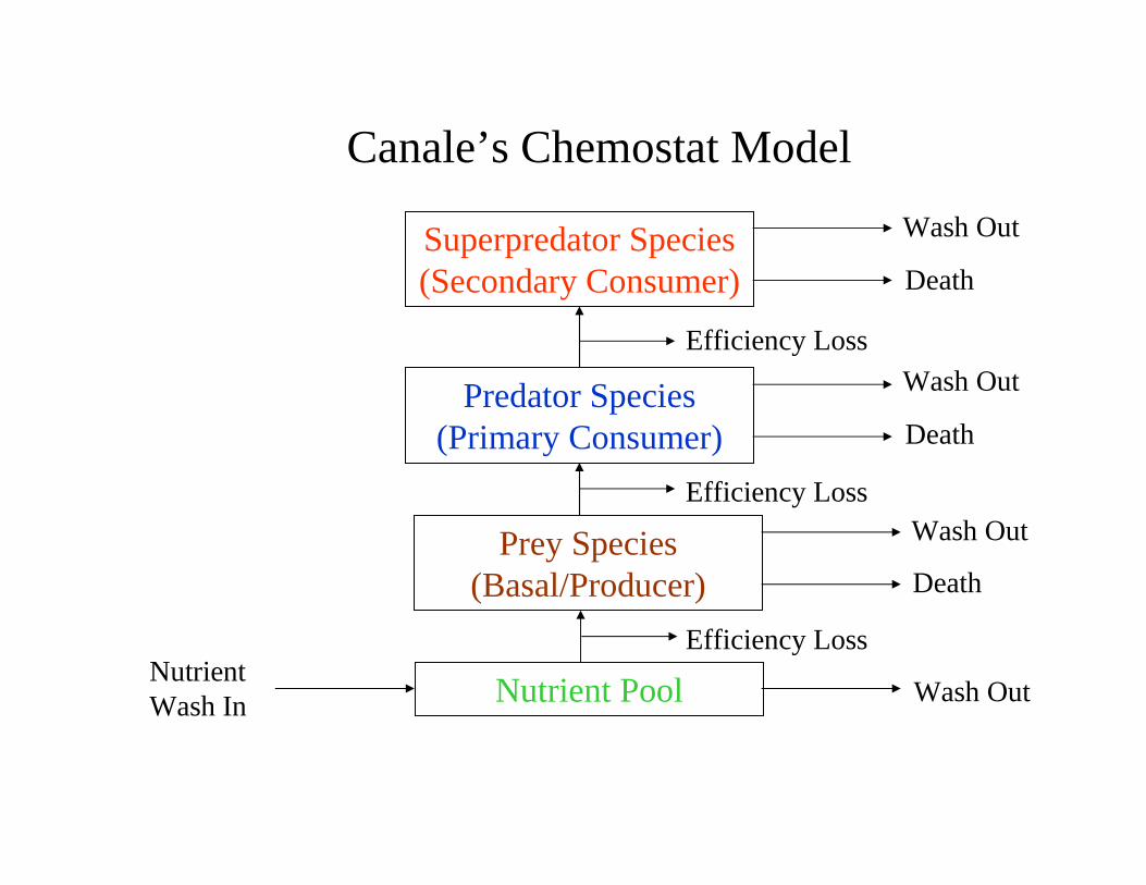
Canale’s Chemostat Model
Nutrient PoolNutrient Wash In
Superpredator Species(Secondary Consumer)
Predator Species(Primary Consumer)
Prey Species(Basal/Producer)
Wash Out
Wash Out
Death
Wash Out
Death
Wash Out
Death
Efficiency Loss
Efficiency Loss
Efficiency Loss
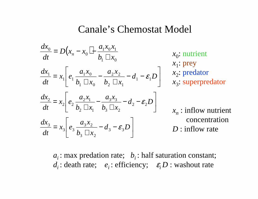
Canale’s Chemostat Model
x0: nutrientx1: preyx2: predatorx3: superpredator
ai : max predation rate; bi : half saturation constant; di : death rate; ei : efficiency; εi D : washout rate
xn : inflow nutrientconcentration
D : inflow rate
( )01
1010
0
xb
xxaxxD
dt
dxn +
−−=
−−
+−
+= Dd
xb
xa
xb
xaex
dt
dx22
23
33
12
1222
2 ε
−−
+= Dd
xb
xaex
dt
dx33
23
2333
3 ε
−−
+−
+= Dd
xb
xa
xb
xaex
dt
dx11
12
22
01
0111
1 ε

Model Computations
• Locate equilibrium pointsand bifurcations of equilibriain the food chain/web model
• A bifurcation is a change in the topological type of the phase portrait as one or more system parameters are varied
– Codimension one: One parameter (α) can be varied
– Codimension two: Two parameters (α, β) can be varied
• Bifurcations of equilibria are located by solving a nonlinear algebraic system consisting of the equilibrium conditions along with one or more augmenting (test) functions
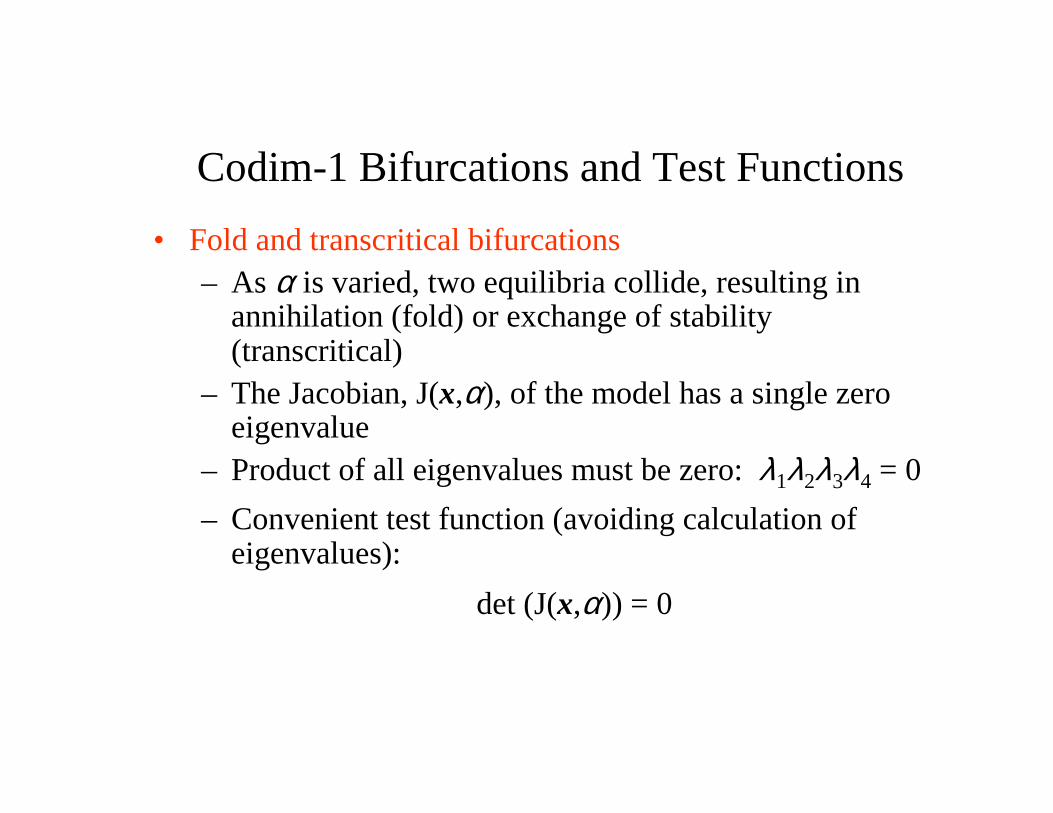
Codim-1 Bifurcations and Test Functions
• Fold and transcritical bifurcations– As α is varied, two equilibria collide, resulting in
annihilation (fold) or exchange of stability (transcritical)
– The Jacobian, J(x,α), of the model has a single zero eigenvalue
– Product of all eigenvalues must be zero: λ1λ2λ3λ4 = 0
– Convenient test function (avoiding calculation of eigenvalues):
det (J(x,α)) = 0
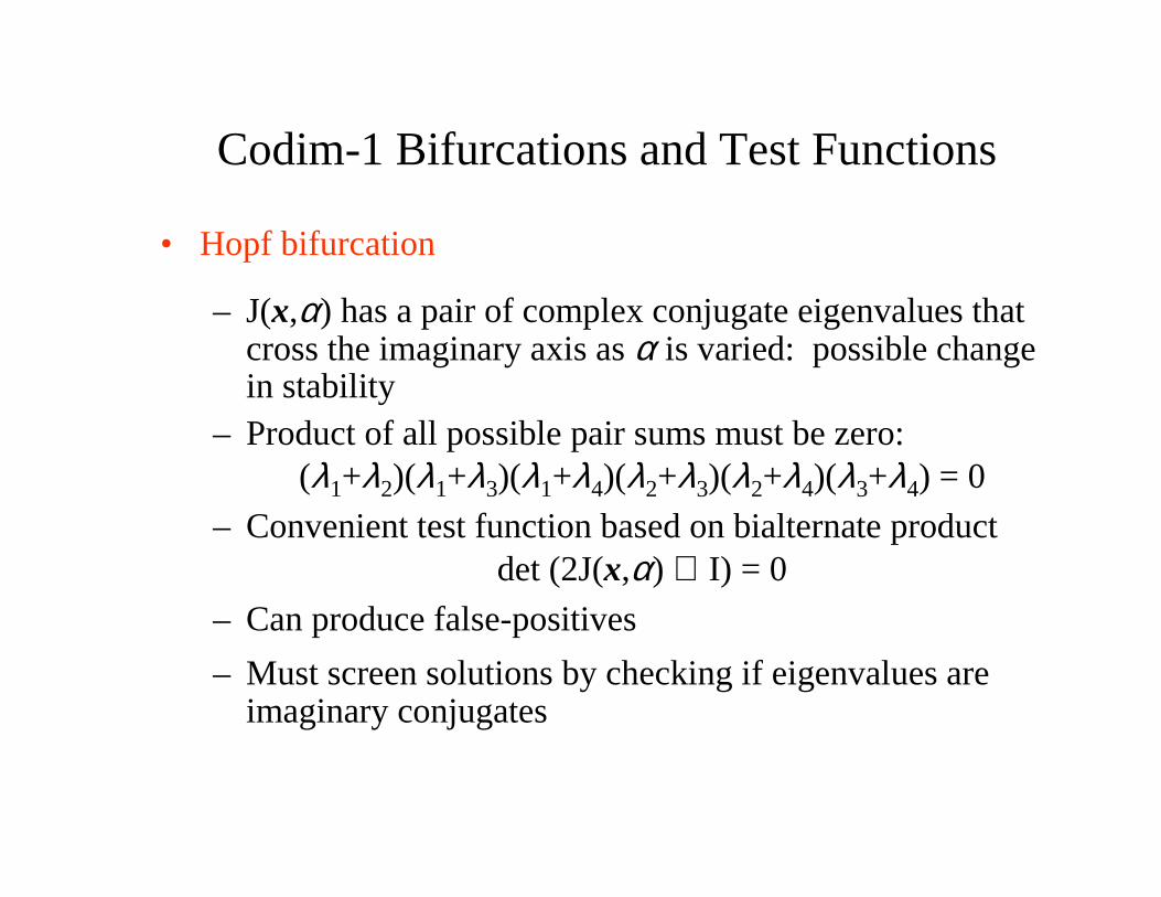
Codim-1 Bifurcations and Test Functions
• Hopf bifurcation
– J(x,α) has a pair of complex conjugate eigenvalues that cross the imaginary axis as α is varied: possible change in stability
– Product of all possible pair sums must be zero:(λ1+λ2)(λ1+λ3)(λ1+λ4)(λ2+λ3)(λ2+λ4)(λ3+λ4) = 0
– Convenient test function based on bialternate productdet (2J(x,α) ⊗ I) = 0
– Can produce false-positives
– Must screen solutions by checking if eigenvalues are imaginary conjugates
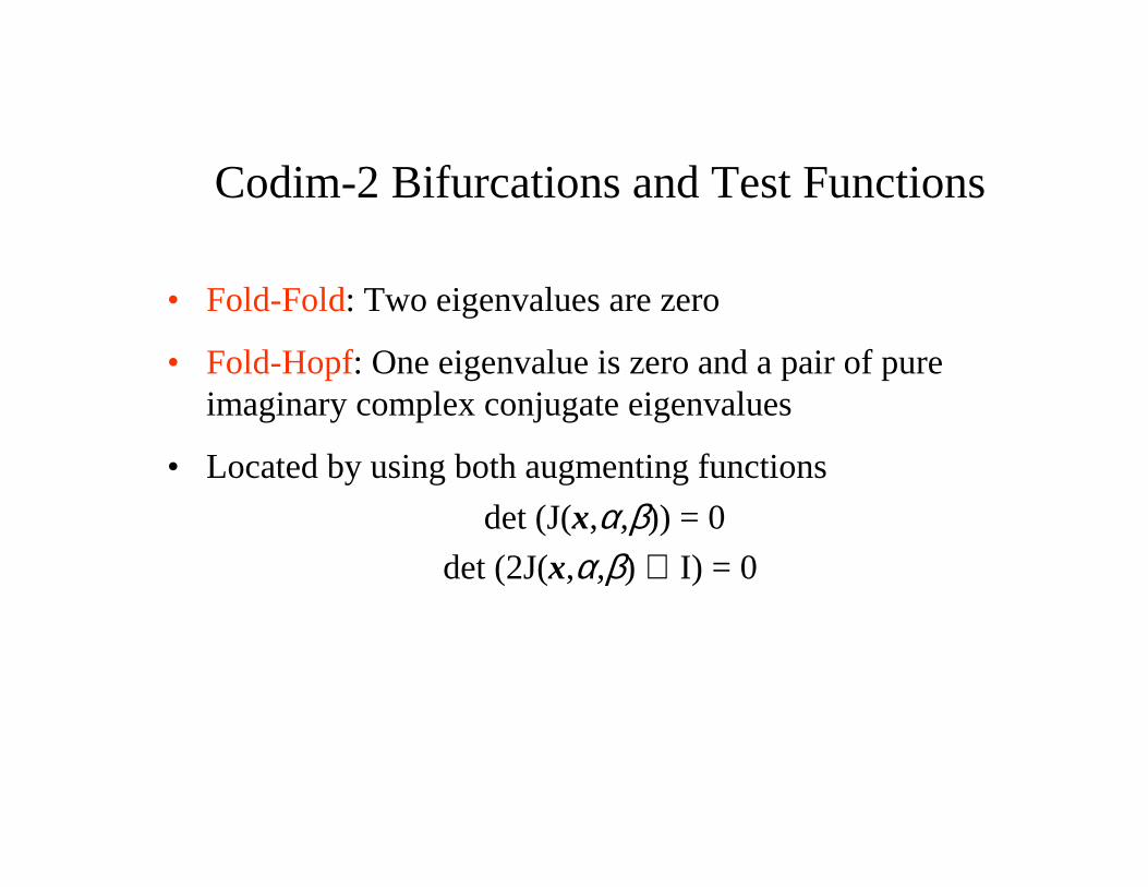
Codim-2 Bifurcations and Test Functions
• Fold-Fold: Two eigenvalues are zero
• Fold-Hopf: One eigenvalue is zero and a pair of pure imaginary complex conjugate eigenvalues
• Located by using both augmenting functions
det (J(x,α,β)) = 0
det (2J(x,α,β) ⊗ I) = 0

Locating Equilibrium States and Bifurcations
• Equilibrium states: Solve equilibrium conditions for x.
• Bifurcations of equilibria: Solve augmented equilibrium conditions for x and α (and β)
• These equation systems may have multiple solutions
• Typically these systems are solved using a continuation-based strategy (e.g., Kuznetsov, 1991; AUTO software)– Initialization dependent
– No guarantee of locating all solution branches
• Interval mathematics provides a method that is:– Initialization independent
– Capable of locating all solution branches with certainty
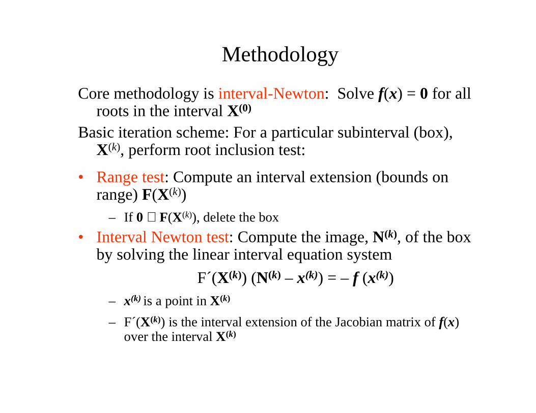
Methodology
Core methodology is interval-Newton: Solve f(x) = 0 for all roots in the interval X(0)
Basic iteration scheme: For a particular subinterval (box), X(k), perform root inclusion test:
• Range test: Compute an interval extension (bounds on range) F(X(k))
– If 0 ∉ F(X(k)), delete the box
• Interval Newton test: Compute the image, N(k), of the box by solving the linear interval equation system
F´(X(k)) (N(k) – x(k)) = – f (x(k))– x(k) is a point inX(k)
– F´(X(k)) is the interval extension of the Jacobian matrix of f(x) over the interval X(k)
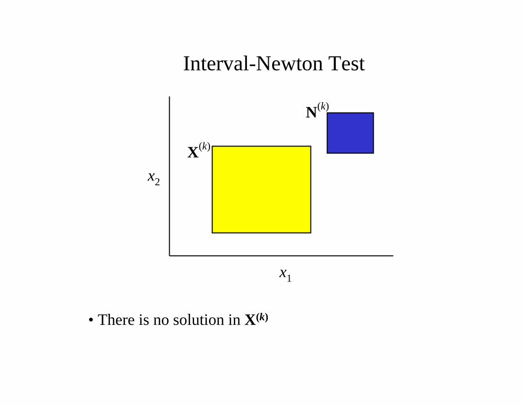
Interval-Newton Test
X(k)
N(k)
x1
x2
• There is no solution in X(k)
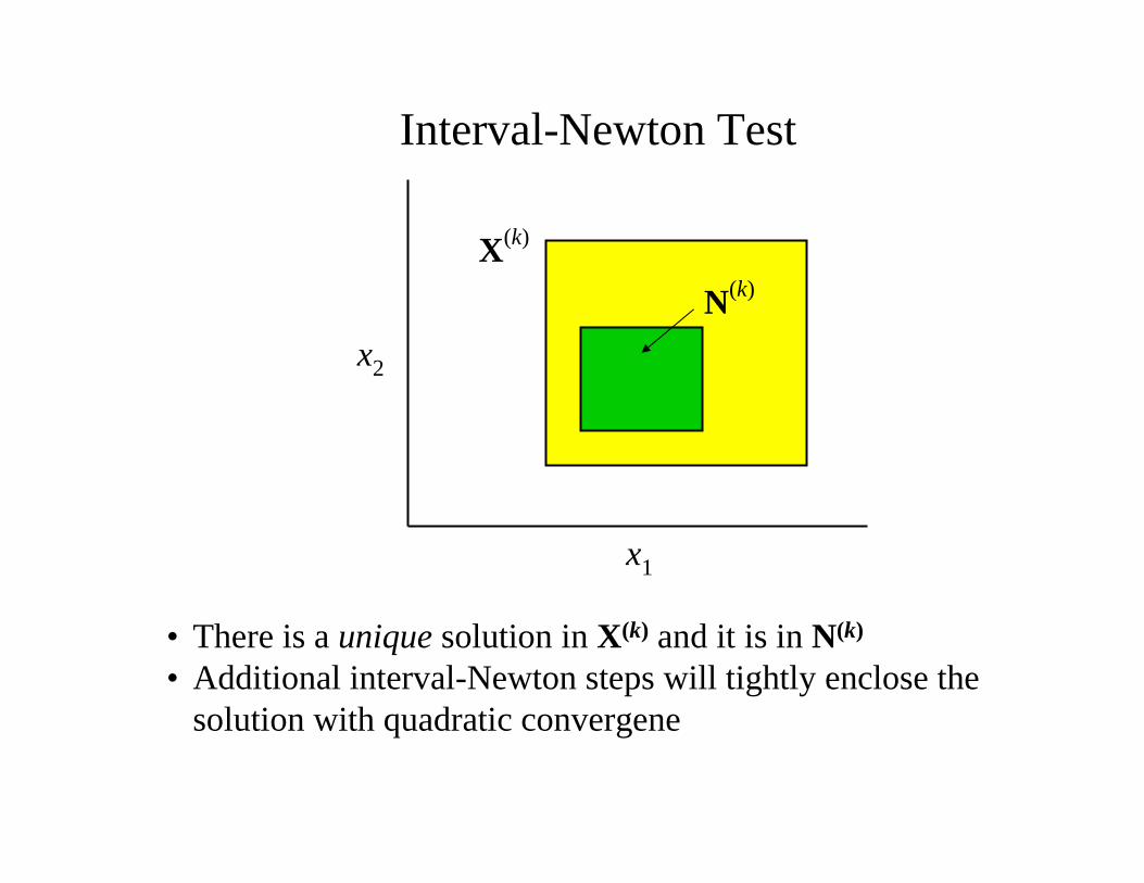
Interval-Newton Test
x1
X(k)
N(k)
x2
• There is a unique solution in X(k) and it is in N(k)
• Additional interval-Newton steps will tightly enclose the solution with quadratic convergene
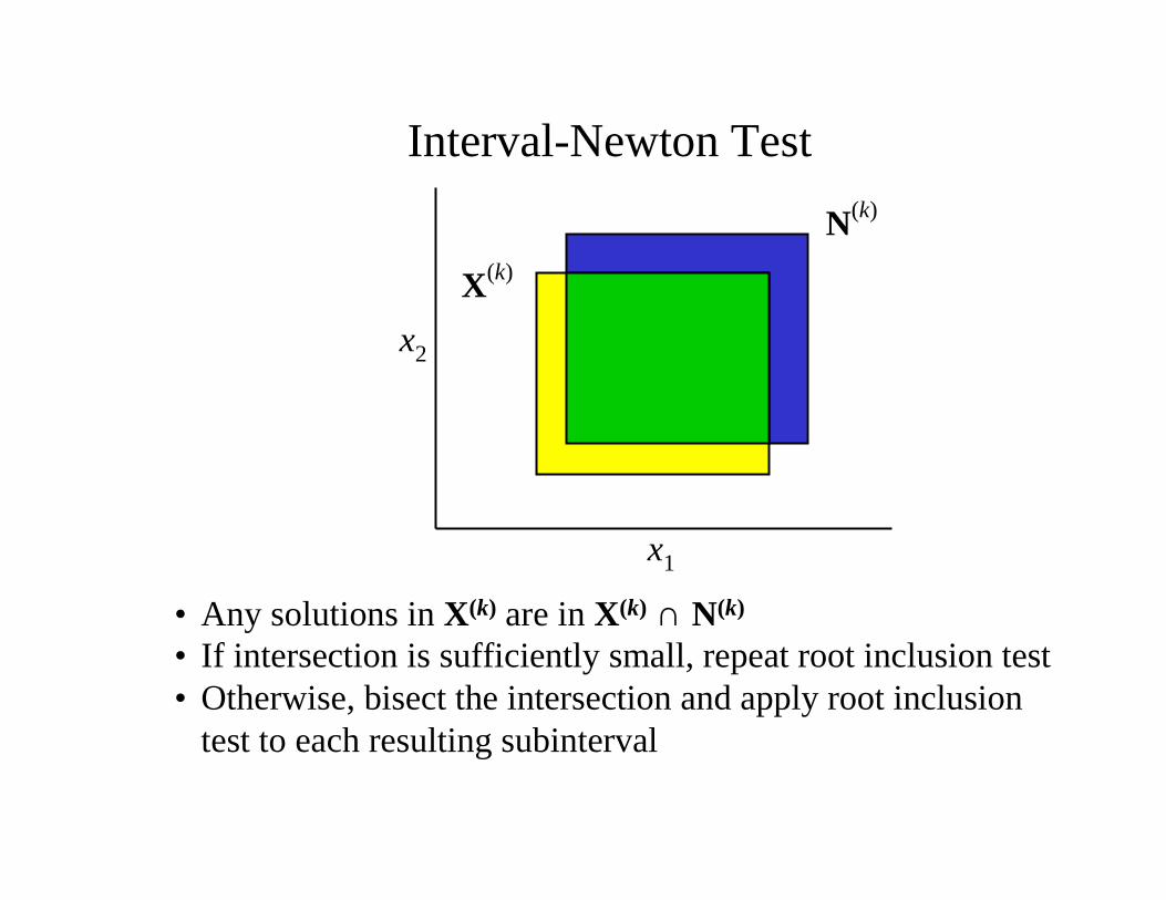
Interval-Newton Test
X(k)
N(k)
x1
x2
• Any solutions in X(k) are in X(k) ∩ N(k)
• If intersection is sufficiently small, repeat root inclusion test• Otherwise, bisect the intersection and apply root inclusion
test to each resulting subinterval
Methodology
Available enhancementsto basic methodology:
• LP-based strategy for computing image N(k) in interval-Newton test (Lin and Stadtherr, 2003, 2004)
– Exact bounds on N(k) (within roundout)
• Constraint propagation (problem specific)
• Tighten interval extensions using known function properties (problem specific)
Generating Solution Diagrams
• Solution branch diagrams(say x vs. xn)– Set xn , use interval-Newton to solve equilibrium conditions for x
– Make small increment in xn and repeat
• Bifurcation diagrams(say xn vs. D)– Set D, solve for values of xn and x at which bifurcations occur
– Make small increment in D and repeat
– Set xn, solve for values of D and x at which bifurcations occur
– Make small increment in xn and repeat
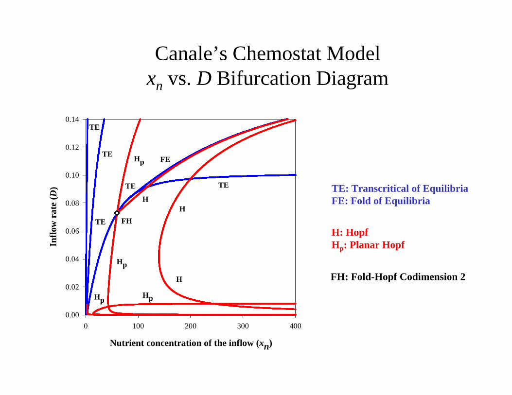
Canale’s Chemostat Modelxn vs. D Bifurcation Diagram
TE: Transcritical of EquilibriaFE: Fold of Equilibria
H: HopfHp: Planar Hopf
FH: Fold-Hopf Codimension 2
Nutrient concentration of the inflow (xn)
0 100 200 300 400
Infl
ow r
ate
( D)
0.00
0.02
0.04
0.06
0.08
0.10
0.12
0.14
Hp
H
H
TE
FE
TE
TE
FH
Hp
H
Hp
Hp
TE TE
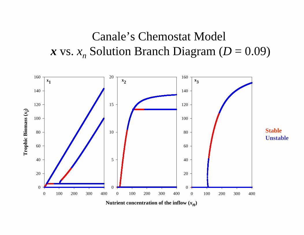
Canale’s Chemostat Modelx vs. xn Solution Branch Diagram (D = 0.09)
Nutrient concentration of the inflow (xn)
0 100 200 300 400
Tro
phic
Bio
mas
s ( x
i)
0
20
40
60
80
100
120
140
160
0 100 200 300 400
0
5
10
15
20
0 100 200 300 400
0
20
40
60
80
100
120
140
160x1 x3x2
StableUnstable
Canale’s Model with Contaminant
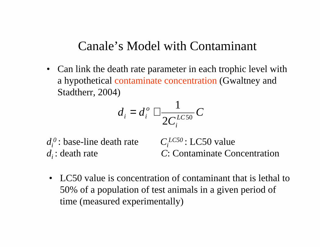
• Can link the death rate parameter in each trophic level with a hypothetical contaminate concentration(Gwaltney and Stadtherr, 2004)
CC
ddLCi
oii 502
1+=
di0 : base-line death rate Ci
LC50 : LC50 value di : death rate C: Contaminate Concentration
• LC50 value is concentration of contaminant that is lethal to 50% of a population of test animals in a given period of time (measured experimentally)
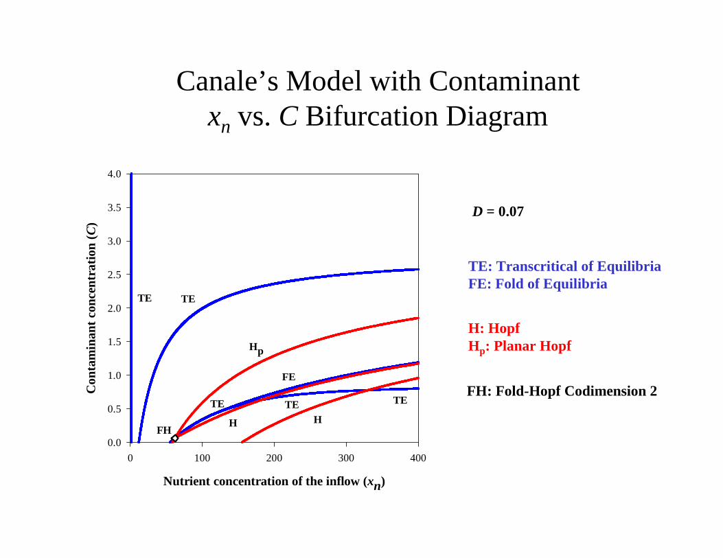
Canale’s Model with Contaminantxn vs. C Bifurcation Diagram
TE: Transcritical of EquilibriaFE: Fold of Equilibria
H: HopfHp: Planar Hopf
FH: Fold-Hopf Codimension 2
D = 0.07
Nutrient concentration of the inflow (xn)
0 100 200 300 400
Con
tam
inan
t co
ncen
trat
ion
(C)
0.0
0.5
1.0
1.5
2.0
2.5
3.0
3.5
4.0
H
TE
FE
TE
TE
FH
Hp
H
TE TE
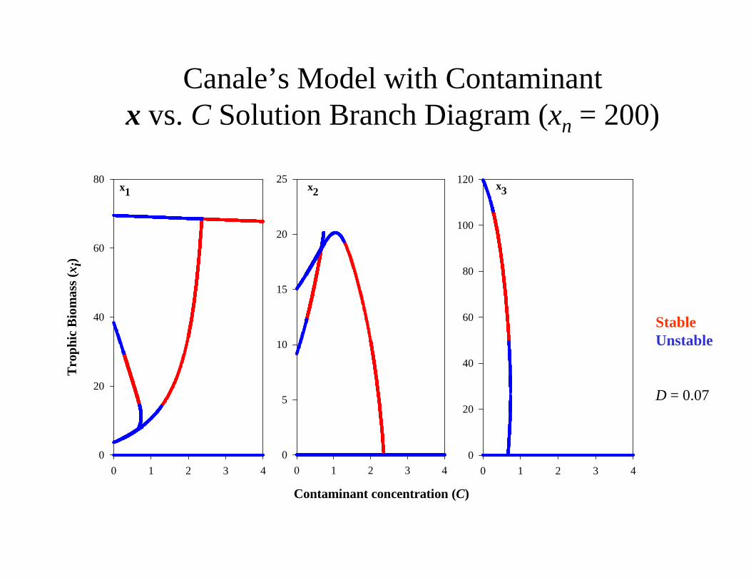
Canale’s Model with Contaminantx vs. C Solution Branch Diagram (xn = 200)
StableUnstable
D = 0.07
Contaminant concentration (C)
0 1 2 3 4
Tro
phic
Bio
mas
s ( x
i)
0
20
40
60
80
0 1 2 3 4
0
5
10
15
20
25
0 1 2 3 4
0
20
40
60
80
100
120x1 x3x2
Concluding Remarks
• Computation times (1.7GHz Xeon/Linux) are reasonable− Average 0.06 s to solve for equilibrium states− Average 15 s to solve for fold/transcritical bifurcations− Average 100 s to solve for Hopf bifurcations
• Using interval methodology, can generate solution branch and bifurcation diagrams with confidence, without need for initialization or a priori insights
• Diagrams can be generated automatically without user intervention to deal with initialization issues
• Applicable to a wide variety of problems in nonlinear dynamics

Acknowledgements
• U.S. Department of Education GAANN Program (P200A010448)
• Arthur J. Schmitt Foundation
• State of Indiana 21st Century Research and Technology Fund (909010455)
• U.S. NSF DMR Program (00-79747)
Recommended