Reduction of Temporal Discretization Error in an Atmospheric General Circulation Model (AGCM)
Final Presentation
Apr. 30, 2013Daisuke [email protected]
Advisor: Prof. Eugenia KalnayDept. of Atmospheric and Oceanic Science,
University of Maryland, College [email protected]

Outline1. Introduction
2. Phase I: Implementation of Lorenz N‐cycleto SPEEDY model
1. Approach2. Algorithms3. Model description4. Stiffness‐problem and semi‐
implicit method5. Semi‐implicit Lorenz N‐cycle6. Code Validation7. Verification: Dynamical‐core test8. Inclusion of Physics &
Comparison of Climatoligies9. Conclusion10. Schedule, planned and actual
3. Phase II: Empirical Characterization of Model Errors
1. Approach2. Algorithm3. Interpolation4. Model Error Bias: results5. Schedule, planned and actual
4. Outcome/Delivarable5. References

Numerical Weather Prediction (NWP):= Initial Value Problem of PDE
Atmospheric Phenomena
Governing Equations
NumericalDiscretization
∂ζ∂t
=1
a(1− µ2)∂FV
∂λ−
1a∂FU
∂µ
− K R(σ)(ζ − [ζ]) − K ν ∇4σ −
22
a2 ζ +dζdt for ci ng
∂D∂t
=1
a(1− µ2)∂FU
∂λ+
1a∂FV
∂µ− ∇2
σ(Φ+ RT̄π+ KE)
− K R(σ)(D − [D ]) − K ν ∇4σ −
22
a2 D
∂T∂t
= −1
a(1− µ2)∂UT∂λ
−1a∂VT∂µ
+ T D
− σ̇∂T∂σ
+ κT∂π∂t
+ vH ·∇σπ+σ̇σ
−K N (σ)(T − [T]) − K h ∇4σ −
22
a2 T +dTdt forci ng
∂π∂t
+ vH ·∇σπ = −D −∂σ̇∂σ
Solve !(Simulate)
(Real Atmosphere)(from JMA website)
Simulated Atmospherefrom http://iprc.soest.hawaii.edu/news/news_2009.php
Hydrodynamic PDE O(109)‐dimensional ODE
from http://www.jma.go.jp/jma/jma‐eng/jma‐center/nwp/nwp‐top.htm
AGCM: Atmospheric General Circulation Model= a computer program which simulates the flow of global atmosphere by numerically integrating the governing fluid dynamical PDEs

Introduction: Motivation
Due to computational restrictions …• most AGCMs adopt low‐order time‐integration schemes, such as
‐ Leap‐frog with Robert‐Asselin filter (1st order)‐ Explicit Backward Euler (aka. Matsuno; 1st order)
• Often, Δt is taken as the largest value for which computational instability is suppressed,
• under the premise that temporal discretization errors are negligible compared to those associated with spatial discretization or Physical Parameterizations.

Introduction: MotivationHowever …• Spatial resolutions become finer and finer as the supercomputers become faster.
• Is the premise that time truncation errors are negligible justified ?
• If not, how can we alleviate such errors ?
Goal of the Project: Reduction of such model errorsApproaches :Phase 1: Use a more accurate scheme with the same
computational costPhase 2: Identify and parameterize the error, and reduce
it using data assimilation

Phase I: Implementation of Lorenz N‐cycle
to SPEEDY model

Phase 1 : A Better integration scheme (Lorenz N‐cycle)
Lorenz (1971) proposed an incredibly smart time‐integration scheme which:• requires only 1 function evaluation per step• but yet (every N steps) it is of ‐ (up to) 4th‐order accuracy (for nonlinear systems)‐ arbitrary order of accuracy (for linear systems)
However, this scheme seems to have remained forgotten. No applications have been made to AGCMs.
Apply Lorenz N‐cycle to an AGCM (Phase 1)

Phase 1: Approach
• Implement Lorenz N‐cycle to an existing AGCM• Implement 4th order Runge‐Kutta (RK4) as well as a reference
• Compare the accuracy and efficiency of the newly introduced schemes with the original scheme
• Perform verification by the Jablonowski‐Williamson (2006) Dynamical‐core Tests

Phase 1: Algorithms
Lorenz N‐cycle(existing) Leap‐frog with Robert‐Asselin Filter 4th order Runge‐Kutta
Memory consumption:2 x dim{model state}
Memory consumption:2 x dim{model state}
Memory consumption:4 x dim{model state}
F‐evaluation: 1 per time step F‐evaluation: 1 per time step F‐evaluation: 4 per time step
accuracy: (N <= 4)O((NΔt)N) (every N steps)
O(NΔt ) (in between)
accuracy: O(Δt )
accuracy: O(Δt4 )
ODE to be solved:

Outline1. Introduction
2. Phase I: Implementation of Lorenz N‐cycleto SPEEDY model
1. Approach2. Algorithms3. Model description4. Stiffness‐problem and semi‐
implicit method5. Semi‐implicit Lorenz N‐cycle6. Code Validation7. Verification: Dynamical‐core test8. Inclusion of Physics &
Comparison of Climatoligies9. Conclusion10. Schedule, planned and actual
3. Phase II: Empirical Characterization of Model Errors
1. Approach2. Algorithm3. Interpolation4. Model Error Bias: results5. Schedule, planned and actual
4. Outcome/Delivarable5. References

AGCM: SPEEDY model
• A fast AGCM with simplified physical parameterizations• Developed in ICTP (Italy) by Drs. F. Molteni and F. Kucharski• Horizontal Discretization:
Spectral Representation with Spherical Harmonicstruncated at total wavenumber 30 (T30) ≈ 400km mesh
• Vertical Discretization: 8‐layers Finite Difference on σ‐coordinate
• Temporal Discretization:Leap‐Frog scheme with Robert‐Asselin Filter (1st order Forward Euler for the physical parameterizations)

The equations solved:the “primitive” equation system (PDEs)on a spherical geometry + parametrized processes
∂ζ∂t
=1
a(1− µ2)∂FV
∂λ−
1a∂FU
∂µ
− K R(σ)(ζ − [ζ]) − K ν ∇4σ −
22
a2 ζ +dζdt for cing
∂D∂t
=1
a(1− µ2)∂FU
∂λ+
1a∂FV
∂µ− ∇2
σ(Φ+ RT̄π+ KE)
− K R(σ)(D − [D ]) − K ν ∇4σ −
22
a2 D
∂T∂t
= −1
a(1− µ2)∂UT∂λ
−1a∂VT∂µ
+ T D
− σ̇∂T∂σ
+ κT∂π∂t
+ vH ·∇σπ+σ̇σ
−K N (σ)(T − [T]) − K h ∇4σ −
22
a2 T +dTdt for cing
∂π∂t
+ vH ·∇σπ = −D −∂σ̇∂σ
ζ ≡1
a(1− µ2)∂V∂λ
−1a∂U∂µ
D ≡1
a(1− µ2)∂U∂λ
+1a
Vµ
F U ≡ (ζ + f )V − σ̇∂U∂σ
−RT
a∂π∂λ
FV ≡ − (ζ + f )U − σ̇∂V∂σ
−RT
a(1− µ2)
∂π∂µ
KE ≡U2 + V 2
2(1− µ2)
vH ·∇ ≡u
acosϕ∂∂λ σ
+va
∂∂ϕ σ
=U
a(1− µ2)∂∂λ σ
+Va
∂∂µ σ
∇2σ ≡
1a2(1− µ2)
∂2
∂λ2 +1a2
∂∂µ
(1− µ2)∂∂µ
.
θ ≡ T (p/ p00)− κ
κ ≡ R/ Cp
Φ ≡ gz
= −σ
1
RTσ
dσ
π ≡ ln ps
σ̇ ≡dσdt
µ ≡ sin ϕ
U ≡ u cosϕ
V ≡ v cosϕ
Dynamical Core
…..
Sub‐grid Parametrizations
T ≡ T̄(σ) + T
σ̇ = − σ∂π∂t
−σ
0Ddσ −
σ
0vH ·∇σπdσ,

Outline1. Introduction
2. Phase I: Implementation of Lorenz N‐cycleto SPEEDY model
1. Approach2. Algorithms3. Model description4. Stiffness‐problem and semi‐
implicit method5. Semi‐implicit Lorenz N‐cycle6. Code Validation7. Verification: Dynamical‐core test8. Inclusion of Physics &
Comparison of Climatoligies9. Conclusion10. Schedule, planned and actual
3. Phase II: Empirical Characterization of Model Errors
1. Approach2. Algorithm3. Interpolation4. Model Error Bias: results5. Schedule, planned and actual
4. Outcome/Delivarable5. References

Stiffness Problem
• The “Primitive” Equations = Stiff system :• Fast but insignificant modes (= gravity waves) are superposed on the slow but meteorologically meaningful modes (= Rossbywaves)
• Due to the CFL condition for the fast modes, we need very small timestepping Δt
Semi‐implicit method (Robert, 1969)

Semi‐Implicit for Leapfrog (1)Formulation
ODE to be solved:
Slow modes Fast modesassumed Linear
Solve this discretized equation
Implicit Explicit

Semi‐Implicit for Leapfrog (2)How to solve
Define:
Substituteto the discretized equation,
Once you get δu, you can integrate the equation by

Outline1. Introduction
2. Phase I: Implementation of Lorenz N‐cycleto SPEEDY model
1. Approach2. Algorithms3. Model description4. Stiffness‐problem and semi‐
implicit method5. Semi‐implicit Lorenz N‐cycle6. Code Validation7. Verification: Dynamical‐core test8. Inclusion of Physics &
Comparison of Climatoligies9. Conclusion10. Schedule, planned and actual
3. Phase II: Empirical Characterization of Model Errors
1. Approach2. Algorithm3. Interpolation4. Model Error Bias: results5. Schedule, planned and actual
4. Outcome/Delivarable5. References

Semi‐implicit Lorenz N‐cycle
Explicit (original) Semi‐implicit

Accuracy(Consistency) & Stability Analysis: Method
• Following Durran (1991, 1999; MWR) and Williamson (2011; MWR), apply semi‐implicit modification to the second term of the equation:
• Examine the modulus of Amplification factor A.• If |A| < 1, the scheme is stable.• Range of interest:
i.e., CFL condition is met for low‐frequency part but is violated for high‐frequency part.

Accuracy(Consistency)
• Truncation Error:
• By taking α=1/2 (Crank‐Nicolson), the scheme becomes 2nd‐order

Plots of |A|‐1 (α=1/2: Crank‐Nicolson)
Leapfrog with R/A filter:Stable almost everywhere
Lorenz 1‐cycle (=Forward Euler):Unstable everywhere
Lorenz 2‐cycle:
Unstable everywhere
Lorenz 3‐cycle:
Absolutely Unstable for
> 1.5
Lorenz 4‐cycle:
Absolutely Unstable for
> 2.7
Stable
Unstable
Unstable UnstableUnstable
Stable Stable
Unstable

Plots of |A|‐1 (α=1: Backward Euler)
Ref:Leapfrog+R/A filter
Lorenz 1‐cycle (=Forward Euler):
Lorenz 2‐cycle: Lorenz 3‐cycle: Lorenz 4‐cycle:
Stable
Unstable Unstable
Stable
Unstable
Stable
Unstable
Stable
Unstable
Stable
Stability is good, but damping is too strong (50%)

Stability for α=1/2: Crank‐NicolsonN=1,…,6
1‐cycle 2‐cycle
3‐cycle 4‐cycle
5‐cycle 6‐cycle
White: stable |A|< 1
Gray: Unstable |A| > 1

Stability for α=1: Backward EulerN=1,…,6
1‐cycle 2‐cycle
3‐cycle 4‐cycle
5‐cycle 6‐cycle
White: stable |A|< 1
Gray: Unstable |A| > 1

Stability: Summary
• Crank‐Nicolson semi‐implicit N‐cycle is unstable for N=1,2
• Stability region is largest for N=4• More unstable than Leapfrog.
• Backward Euler semi‐implicit N‐cycle is more stable, but damping is too strong

Outline1. Introduction
2. Phase I: Implementation of Lorenz N‐cycleto SPEEDY model
1. Approach2. Algorithms3. Model description4. Stiffness‐problem and semi‐
implicit method5. Semi‐implicit Lorenz N‐cycle6. Code Validation7. Verification: Dynamical‐core test8. Inclusion of Physics &
Comparison of Climatoligies9. Conclusion10. Schedule, planned and actual
3. Phase II: Empirical Characterization of Model Errors
1. Approach2. Algorithm3. Interpolation4. Model Error Bias: results5. Schedule, planned and actual
4. Outcome/Delivarable5. References

Code Validation: Idea
• Lorenz N‐cycle:– Lorenz 1‐cycle is equivalent to Forward Euler, which is built‐in in the SPEEDY model.
– Compare Lorenz 1‐cycle with Forward Euler.
• RK4 :– For a linear system, RK4 with 4Δt is equivalent to Lorenz 4‐cycle with Δt.
– Remove all nonlinear terms from SPEEDY and Compare RK4 (4Δt) with Lorenz 4‐cycle (Δt).

Code Validation: Results
• Outputs of single step integrations of Lorenz 1‐cycle and Forward Euler from the same initial condition are compared using UNIX diff command. – Result no difference (Success)!
• Similarly, outputs of single step integration of RK4 and four‐step integration of Lorenz 4‐cycle from the same initial condition are compared using UNIX diff command. – Result no difference (Success)!

Outline1. Introduction
2. Phase I: Implementation of Lorenz N‐cycleto SPEEDY model
1. Approach2. Algorithms3. Model description4. Stiffness‐problem and semi‐
implicit method5. Semi‐implicit Lorenz N‐cycle6. Code Validation7. Verification: Dynamical‐core test8. Inclusion of Physics &
Comparison of Climatoligies9. Conclusion10. Schedule, planned and actual
3. Phase II: Empirical Characterization of Model Errors
1. Approach2. Algorithm3. Interpolation4. Model Error Bias: results5. Schedule, planned and actual
4. Outcome/Delivarable5. References

Verification: Dynamical‐Core test cases
• Standardized tests for dynamical cores of AGCM proposed by Jablonowski and Williamson (2006) which consists of two tests:
1. Steady‐State test:– A model is integrated from an analytical steady‐state
solution of the primitive equation– The model is evaluated by how well it can keep the
steady‐state intact.2. Baroclinic‐Wave test:
– The model is integrated with initial and boundary conditions which is designed to produce an idealized baroclinic wave (= extratropic cyclones and highs)

Baroclinic‐wave Test: Result (Lorenz 4‐cycle)
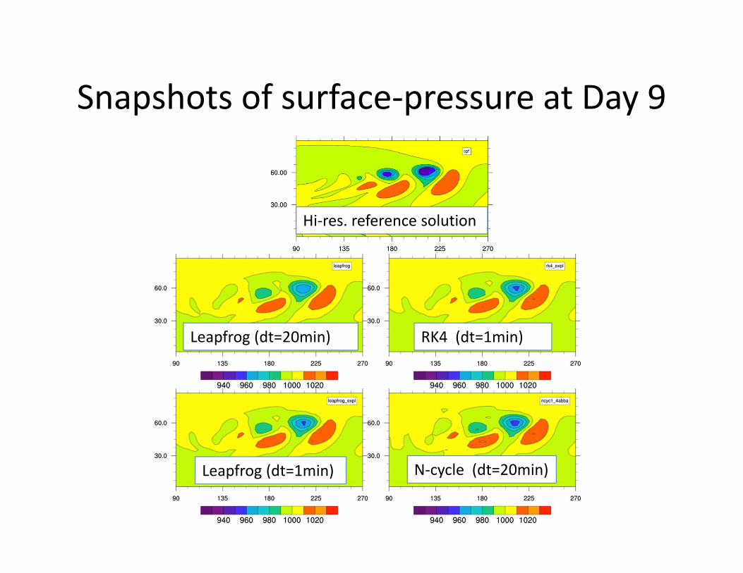
Snapshots of surface‐pressure at Day 9
Hi‐res. reference solution
Leapfrog (dt=20min)
Leapfrog (dt=1min)
RK4 (dt=1min)
N‐cycle (dt=20min)

Order estimation
• Lorenz 4‐cycle is supposedly of 4th‐order, while Leapfrog (with R/A filter) is only of 1st‐order
• Confirm this by plotting L2 error vs. Δt on a log‐log plane.
• Experimental set‐up: Jablonowski‐Williamson baroclinic‐wave test
• Measure of the error: difference in surface pressure with respect to the reference solution produced by RK4 with Δt=0.5min in L2 ‐norm

Result : L2(Ps) at t=3days
N‐cycle +CN
Leapfrog +CN
N‐cycle +BE
Leapfrog +BE

Result : L2(Ps) at t=5days
N‐cycle +CN
Leapfrog +CN
N‐cycle +BE
Leapfrog +BE

Result : L2(Ps) at t=10days
N‐cycle +CN
Leapfrog +CN
N‐cycle +BE
Leapfrog +BE

Dynamical‐core testSummary of the results
• For Δt ≤ 10min, the order of Lorenz 4‐cycle is 3rd 4th
• For a large Δt, A‐B‐B‐A cycle is inferior to version A or version B, which contradicts with Lorenz (1971)’s claim.
• Possible reasons:– Cancellation of truncation errors of version A and B does may hold because of the introduction of semi‐implicit method.
– Cancellation between A and B itself is not attained for the AGCM.
– A‐B‐B‐A cycle is more unstable for nonlinear models than A‐only or B‐only.
To be examined

Outline1. Introduction
2. Phase I: Implementation of Lorenz N‐cycleto SPEEDY model
1. Approach2. Algorithms3. Model description4. Stiffness‐problem and semi‐
implicit method5. Semi‐implicit Lorenz N‐cycle6. Code Validation7. Verification: Dynamical‐core test8. Inclusion of Physics &
Comparison of Climatoligies9. Conclusion10. Schedule, planned and actual
3. Phase II: Empirical Characterization of Model Errors
1. Approach2. Algorithm3. Interpolation4. Model Error Bias: results5. Schedule, planned and actual
4. Outcome/Delivarable5. References

Inclusion of Physics
• Having proved that N‐cycle works without physical parameterizations, I next tried to include physics in the N‐cycle SPEEDY model.
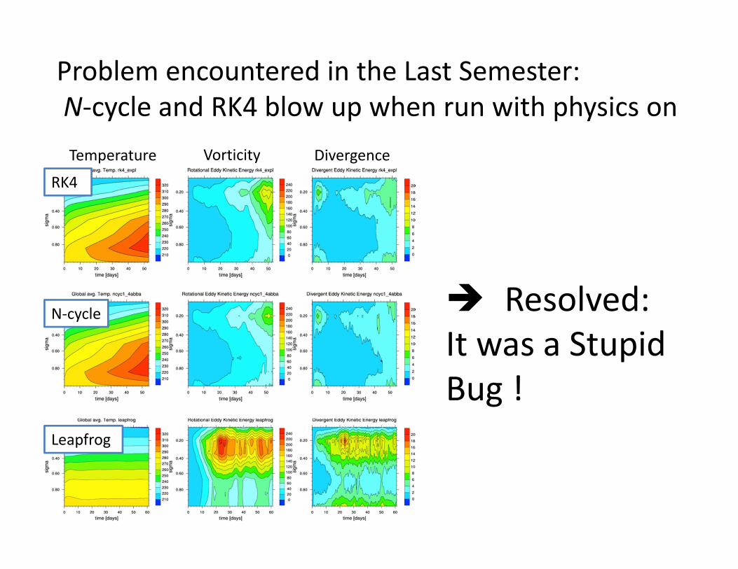
Problem encountered in the Last Semester:N‐cycle and RK4 blow up when run with physics onTemperature Vorticity Divergence
RK4
N‐cycle
Leapfrog
Resolved: It was a Stupid Bug !

Stability• After fixing the bug, I tried to find the largest Δt with which the N‐
cycle can integrated stably.
Bad news: the largest stable Δt• for N‐cycle : 15 mins, whereas• for Leapfrog: 40mins.
Possible remedy (with some accuracy degradation) :• the largest stable Δt can be made 30mins• by using Backward Euler for the gravity‐wave part (instead of the
default Crank‐Nicolson)
• N‐cycle can be integrated with Δt=15mins. for at least 100 years (=3,504,000 steps)

Comparison of Climatology (= long‐term mean)
• In climate application, it is important that the long‐term mean of the atmospheric state (called climatology) does not change.
• Statistically compared the climatologies using Welch’s t‐test.
• Examined Climatologies:two seasons (DJF: 12‐2 and JJA: 6‐8), each from 3 models:– Leapfrog with dt=40mins (default)– 4‐cycle (Crank‐Nicolson for gravity‐wave) dt=15mins– 4‐cycle (Backward Euler for gravity‐wave) dt=30mins

t‐test for the difference of climatologies
• Experimental design:– Run all the models from the same initial condition (state of rest)
– Integrate for 30 years.– Discard the first 10 years as a spin‐up.– Use the remaining 20 years as the samples.
• Null‐hypothesis:climatologies (= sample means) are taken from the
same population.• The probability of the differences between two sampled climatologies being larger than the observed difference under the null‐hypothesis is computed.
• If this probability is larger than 95%, then the null‐hypothesis is not rejected.
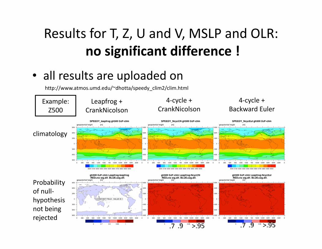
Results for T, Z, U and V, MSLP and OLR:no significant difference !
• all results are uploaded on http://www.atmos.umd.edu/~dhotta/speedy_clim2/clim.html
4‐cycle + CrankNicolson
4‐cycle + Backward Euler
Leapfrog + CrankNicolson
climatology
Probabilityof null‐hypothesis not being rejected
Example:Z500
>.95.9.7 >.95.9.7

Conclusion for Phase I
• Designed semi‐implicit version of N‐cycle– Analyzed stability using a toy‐model– 4‐cycle is the most stable– For semi‐implicit method, Crank‐Nicolson is more accurate than Backward‐Euler but is more unstable
• Verification through Dynamical‐Core test:– 4‐cycle with Crank‐Nicolson exhibits order‐of‐accuracy which is higher (2nd ~ 3rd) than filtered Leapfrog (1st‐order)

Schedule for Phase 1: Planned and Actual
Planned• Implement RK4 and N‐cycle, Nov.• Write the mid‐year report,
prepare the oral presentation, Dec.
• Switch‐off physical parameterizations, prepare flat topography, Jan.
• perform the dynamical core tests. Feb.
Actual• Formulate semi‐implicit N‐cycle,
Oct.• Implement RK4 and N‐cycle, Nov.• Switch‐off physical
parameterizations, prepare flat topography, Dec.
• perform the dynamical core tests, Dec.
• Write the mid‐year report, prepare the oral presentation, Dec.
• Coded a bug, and fixed the bug, Jan. (winter break)
• Compare climatologies, performed statistical test, Feb.
Phase II:Empirical characterization of Model
Errors

Outline1. Introduction
2. Phase I: Implementation of Lorenz N‐cycleto SPEEDY model
1. Approach2. Algorithms3. Model description4. Stiffness‐problem and semi‐
implicit method5. Semi‐implicit Lorenz N‐cycle6. Code Validation7. Verification: Dynamical‐core test8. Inclusion of Physics &
Comparison of Climatoligies9. Conclusion10. Schedule, planned and actual
3. Phase II: Empirical Characterization of Model Errors
1. Approach2. Algorithm3. Interpolation4. Model Error Bias: results5. Schedule, planned and actual
4. Outcome/Delivarable5. References

Phase 2: Approach• Objective: Characterize the model errors due to temporal
discretizations
• Take the Truth from NCEP/NCAR reanalysis (Kalnay et al. 1996)
NCEP=National Centers for Environmental PredictionNCAR=National Center for Atmospheric Research
• Extract model errors by applying the method of Danforth et al. (2007) to the models with:
1. the original scheme (Leap‐Frog; MLF)2. Lorenz N‐cycle scheme (MNCYC)
• (time permitting) Correct the model errors on‐line during the course of model integration ( Phase 3&4)

Phase 2: Algorithm
1. Generate initial values from the Truth (NCEP/NCAR reanalysis)
2. Perform short‐range forecasts using the 2 models (MLF, MNCYC4) from the initial conditions
3. find the bias of the model errors for each model4. Build the covariance matrix
5. Extract the dominant modes by conducting SVD

Interpolation from NCEP/NCAR grid to SPEEDY grid
• Obtained the original code (used in Danforth et.al (2007)) and wrote a code that does exactly the same operation
• Original code: – written in MatLab script– performs Simple linear interpolation in 3D
• My code:– wrote in NCL (NCAR Command Language)– Basically a line‐by‐line translation from MatLab to NCL
• Validation:– Method:
• produce data on SPEEDY grid from NCEP/NCAR data using the original code and my code
• compare the two outputs, one from the original, the other from my code– Result: the two outputs agreed within single‐precision rounding error

Outline1. Introduction
2. Phase I: Implementation of Lorenz N‐cycleto SPEEDY model
1. Approach2. Algorithms3. Model description4. Stiffness‐problem and semi‐
implicit method5. Semi‐implicit Lorenz N‐cycle6. Code Validation7. Verification: Dynamical‐core test8. Inclusion of Physics &
Comparison of Climatoligies9. Conclusion10. Schedule, planned and actual
3. Phase II: Empirical Characterization of Model Errors
1. Approach2. Algorithm3. Interpolation4. Model Error Bias: results5. Schedule, planned and actual
4. Outcome/Delivarable5. References

Model Error Bias : ResultsZonal wind at 200hPa
From Danforth et.al (2007)

Model Error Bias : ResultsTemperature at 850hPa
From Danforth et.al (2007)
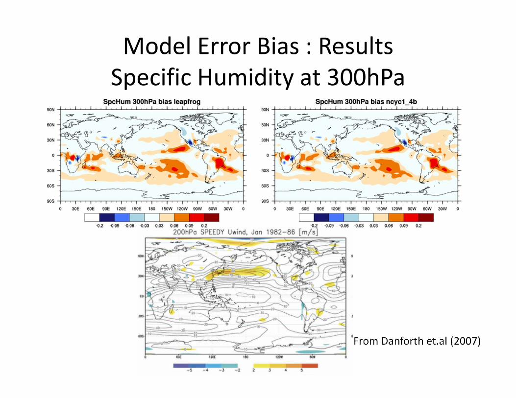
Model Error Bias : ResultsSpecific Humidity at 300hPa
From Danforth et.al (2007)
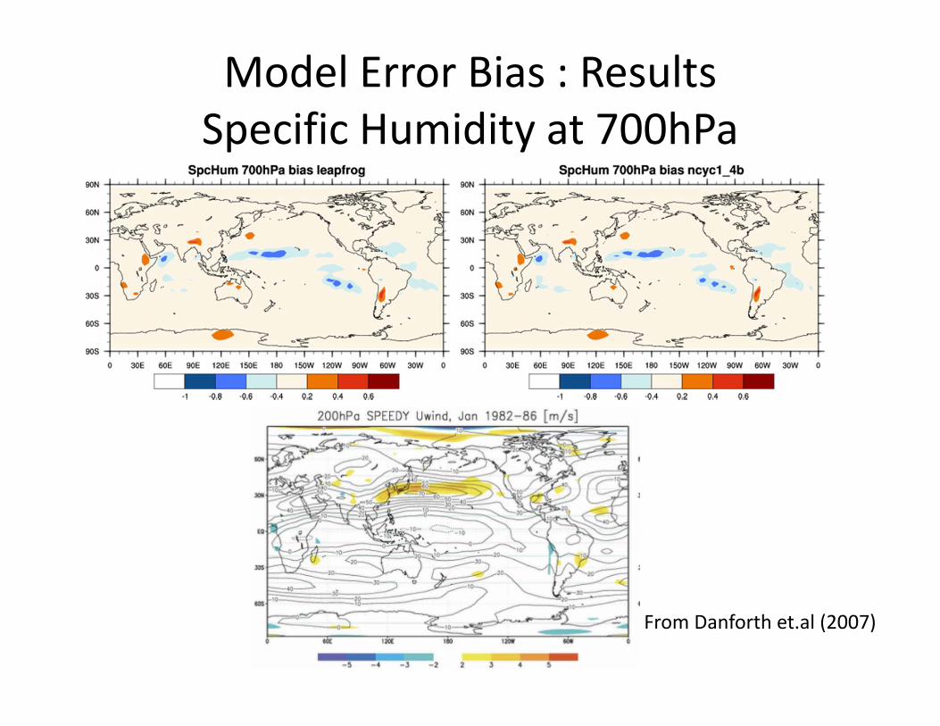
Model Error Bias : ResultsSpecific Humidity at 700hPa
From Danforth et.al (2007)
Model Error Bias : Summary
• For all variables, Leapfrog and N‐cycle produce almost identical bias pattern• Interpretation: bias is dominated by the model’s deficiencies associated with physical parameterizations
• They are consistent with Danforth et.al (2007)

Plan for Phase II
In Danforth et.al (2007),1. Error samples {δx} are produced with the
original model M2. Bias <δx> is computed3. The model is modified by incorporating
nudging to ‐<δx> to yield M+
4. Error samples {δx+} are resampled using the de‐biased model M+
5. Diurnal errors are extracted from {δx+} by performing EOF analysis and retaining the first two dominant modes
6. The de‐biased model M+ is again modified by incorporating nudging to negative of diurnal biases to yield M++
7. Error samples {δx++} are again resampled using M++
8. Perform SVD analysis to extract dominant co‐variation of model error δx++ and the anomaly of the model states
while, in my original plan, 1. Error samples {δx} are produced with the
original model M2. Bias <δx> is computed3. The model is modified by incorporating
nudging to ‐<δx> to yield M+
4. Error samples {δx+} are resampled using the de‐biased model M+
5. Diurnal errors are extracted from {δx+} by performing EOF analysis and retaining the first two dominant modes
6. The de‐biased model M+ is again modified by incorporating nudging to negative of diurnal biases to yield M++
7. Error samples {δx++} are again resampled using M++
3. Perform SVD analysis to extract dominant co‐variation of model error δx++ and the anomaly of the model states
4. Validation: Results are compared with Danforth et.al (2007)

Plan for Phase II
• Danforth et.al (2007) involves much more tricks than I originally planned.
• Reproducing all the procedures in Danforth et.al (2007) is impossible given that I have only 2‐weeks left.
• I continue the original plan, but modify the Validation part.
• New Validation: – Check orthogonality between the extracted modes

Conclusion for Phase II• Generated samples of model error• Computed biases for Leapfrog and Lorenz 4‐cycle, compared them with Danforth et.al (2007)
Result:– No significant bias improvements by using a better temporal scheme. Perhaps dominated by physics errors
– Consistent with Danforth et.al (2007)
• TODO (in two weeks): – SVD analysis to identify the dominant co‐varying modes between model state anomaly and model error
– Comparison with Danforth et.al (2007)

Schedule for Phase 2: Planned and Actual
Planned• Generate initial values from the
NCEP/NCAR reanalysis, end of Feb.
• Compute the bias, Mar.• Plot the bias and compare It with
Danforth et.al, Apr. ( Now I’m here)
• Code and test a program for SVD, May.
• Compare the model errors for the new and the original schemes, May.
• Write the final report (paper draft), May.
Actual• Generate initial values from
the NCEP/NCAR reanalysis, end of Feb.
• build the bias and covariance matrix, Mar.
• Code and test a program for SVD, Apr.
• Compare the model errors for the new and the original schemes, May.
• Write the final report (paper draft), May.

Outcome/DeliverablesPhase 1:• Upgraded code for SPEEDY model‐ subroutines for Lorenz N‐cycle and 4th order Runge‐Kutta
• Test‐case results for the SPEEDY model (both for the original scheme and the new schemes)
Available at https://code.google.com/p/speedy‐lorenz‐ncycle/
Phase 2:• Archive of the model errors• Bias of model errors • Pairs of Singular Vectors for the model state and the model error• Code for performing SVD
✔
✔
✔✔
To be completed in two weeks

BibliographyLorenz N‐cycle• Lorenz, Edward N., 1971: An N‐cycle time‐differencing scheme for stepwise numerical integration. Mon. Wea. Rev.,
99, 644–648.
SPEEDY model• Molteni, Franco, 2003: Atmospheric simulations using a GCM with simplified
physical parameterizations. I. Model climatology and variability in multi‐decadal experiments. Clim. Dyn., 20, 175‐191.
• Kucharski F, Molteni F, and Bracco A, 2006: Decadal interactions between the western tropical Pacific and the North Atlantic Oscillation. Clim. Dyn., 26, 79‐91
SPEEDY‐LETKF• Miyoshi, T., 2005: Ensemble Kalman filter experiments with a primitive‐equation global model. Ph.D. dissertation,
University of Maryland, College Park, 197pp.
Atmospheric GCM Dynamical Core test cases• Jablonowski, C. and D. L. Williamson 2006: A baroclinic instability test case for atmospheric model dynamical
cores, Q. J. R. Metorol. Soc., 132, 2943‐2975
NCEP/NCAR reanalysis• Kalnay, E., and Coauthors, 1996: The NCEP/NCAR 40‐Year Reanalysis Project. Bull. Amer. Meteor. Soc., 77, 437–471.
Model Error Correction• Danforth, Christopher M., Eugenia Kalnay, Takemasa Miyoshi, 2007: Estimating and Correcting Global Weather
Model Error. Mon. Wea. Rev., 135, 281–299. • Danforth, Christopher M., Eugenia Kalnay, 2008: Using Singular Value Decomposition to Parameterize State‐
Dependent Model Errors. J. Atmos. Sci., 65, 1467–1478.

back‐up slides

Swinging‐pendulum problem• A simple nonlinear test‐bed
for semi‐implicit schemes.• Fast oscillation = elastic
spring• Slow oscillation = pendulum• Fast mode is treated
implicitly, slow mode explicitly.
• For this test, I use Δt=0.075 which givesωLOWΔt=0.225, ωHIGHΔt=2.25,
From Williams (2011)
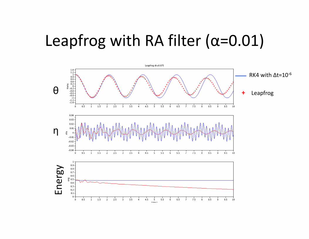
Leapfrog with RA filter (α=0.01)
RK4 with Δt=10‐6
+ Leapfrogθ
η
Energy

4‐cycle with semi‐implicit correction on every 4 steps (Crank‐Nicolson)
θ
η
Energy
RK4 with Δt=10‐6
+ Leapfrog

4‐cycle with semi‐implicit correction on every 4 steps (Backward)
stable but very dissipative
θ
η
Energy
RK4 with Δt=10‐6
+ Leapfrog

4‐cycle with semi‐implicit correction on every time step unstable
θ
η
Energy
RK4 with Δt=10‐6
+ Leapfrog

Explicit 4‐cycle unstable
θ
η
Energy
RK4 with Δt=10‐6
+ Leapfrog
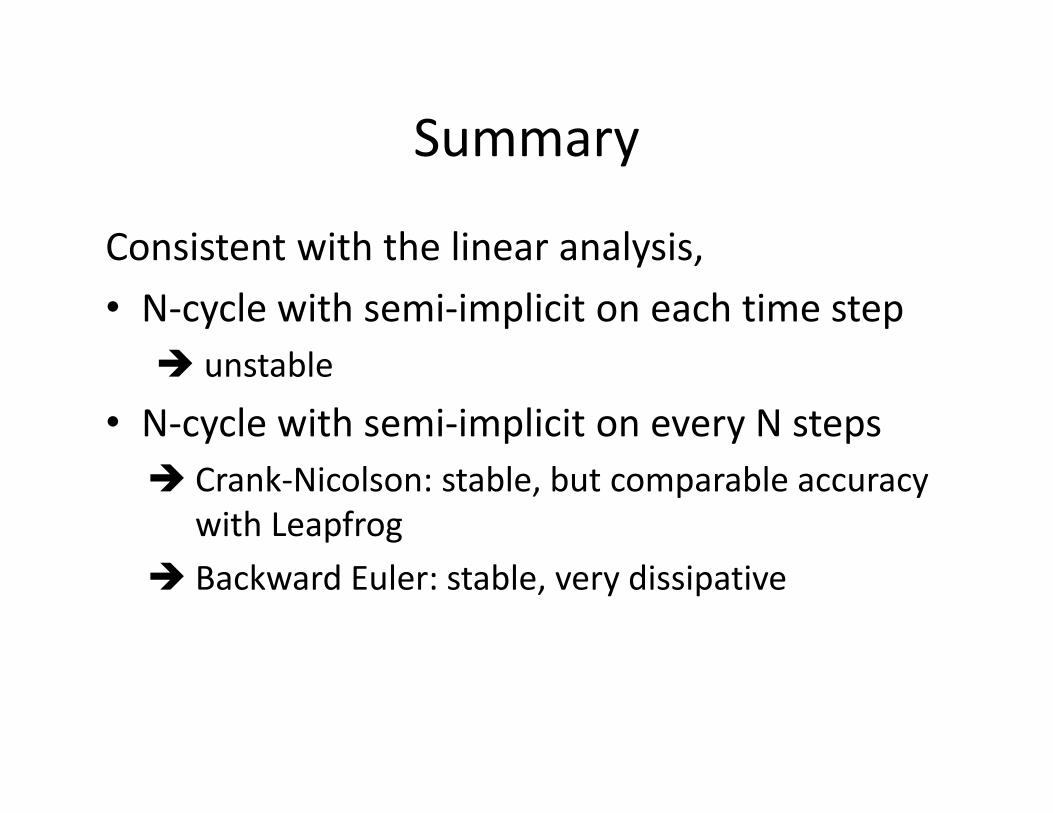
Summary
Consistent with the linear analysis,• N‐cycle with semi‐implicit on each time step unstable
• N‐cycle with semi‐implicit on every N steps Crank‐Nicolson: stable, but comparable accuracy
with Leapfrog Backward Euler: stable, very dissipative

Reference:
• Williams, P. D. 2011: The RAW Filter: An Improvement to the Robert–Asselin Filter in Semi‐Implicit Integrations, Mon. Weath. Rev., 139, 1996‐‐2007

Runge‐Kutta 4th‐order scheme with semi‐implicit correction
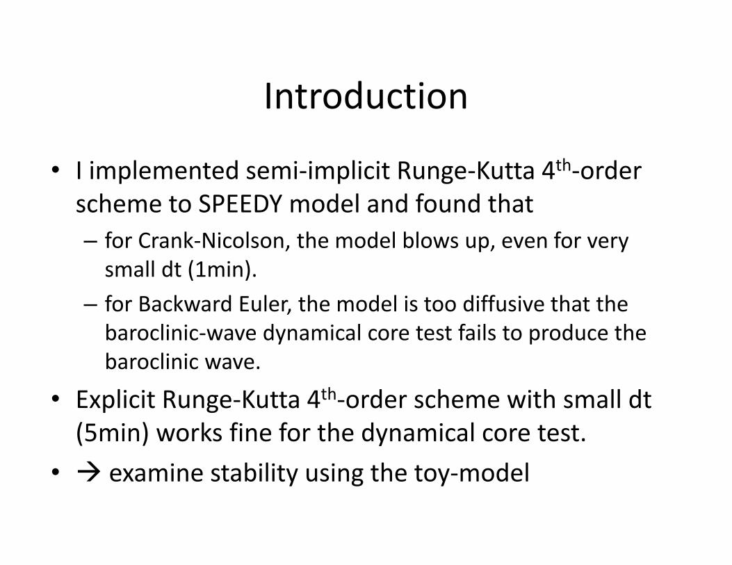
Introduction
• I implemented semi‐implicit Runge‐Kutta 4th‐order scheme to SPEEDY model and found that – for Crank‐Nicolson, the model blows up, even for very small dt (1min).
– for Backward Euler, the model is too diffusive that the baroclinic‐wave dynamical core test fails to produce the baroclinic wave.
• Explicit Runge‐Kutta 4th‐order scheme with small dt(5min) works fine for the dynamical core test.
• examine stability using the toy‐model

Method• Following Durran (1991, 1999; MWR) and Williamson (2011; MWR), apply semi‐implicit modification to the second term of the equation:
• Examine the modulus of Amplification factor A.• If |A| < 1, the scheme is stable.• Range of interest:
i.e., CFL condition is met for low‐frequency part but is violated for high‐frequency part.

Algorithm: RK4 for ωL , Crank‐Nicolson for ωH
Truncation Error:
the accuracy is only 1st order

Plot of |A|‐1β=1/2: Crank‐Nicolson‐> Absolutely unstable
β=1: backward Euler‐> Absolutely stable,but extremely dissipative
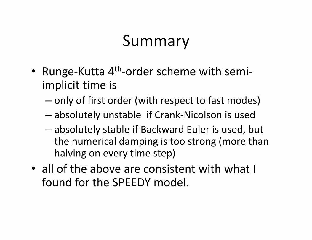
Summary
• Runge‐Kutta 4th‐order scheme with semi‐implicit time is– only of first order (with respect to fast modes)– absolutely unstable if Crank‐Nicolson is used– absolutely stable if Backward Euler is used, but the numerical damping is too strong (more than halving on every time step)
• all of the above are consistent with what I found for the SPEEDY model.

Conclusion
• Runge‐Kutta 4th‐order scheme with semi‐implicit time‐stepping for gravity waves is impossible (either unstable or too dissipative)
• The accuracy becomes only of 1st order.
• Since the motivation for implementing Runge‐Kutta 4th‐order scheme is to produce a reference solution, I will not try to resolve this issue, and use the explicit scheme with small dt.

Stability analysis of Forward Euler “split physics” for Leapfrog, Lorenz
4‐cycle and RK4
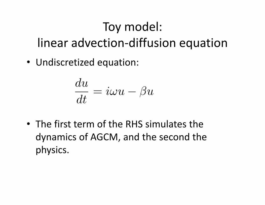
Toy model: linear advection‐diffusion equation
• Undiscretized equation:
• The first term of the RHS simulates the dynamics of AGCM, and the second the physics.

Discretization: Leapfrog(dyn) + Euler(phys)
• Discretized equation:
• The amplification factor A satisfies the following equation:
• (+) and (‐) correspond, respectively, to physical and computational modes.
• The scheme is stable if the maximum of the moduli of them is less than 1.

Discretization: Leapfrog for both dyn & phys
• Discretized equation:
• The amplification factor A satisfies the following equation:
• (+) and (‐) correspond, respectively, to physical and computational modes.
• The scheme is stable if the maximum of the moduli of them is less than 1.
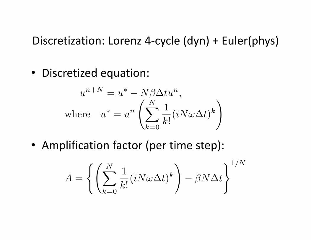
Discretization: Lorenz 4‐cycle (dyn) + Euler(phys)
• Discretized equation:
• Amplification factor (per time step):

Discretization: Lorenz 4‐cycle for both dyn & phys
• Discretized equation:
• Amplification factor (per time step):
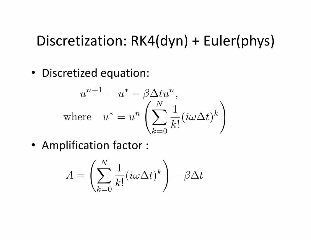
Discretization: RK4(dyn) + Euler(phys)
• Discretized equation:
• Amplification factor :

Discretization: RK4 for both dyn&phys
• Discretized equation:
• Amplification factor (per time step):

Leapfrog:“split physics” stabilizes the otherwise
absolutely unstable schemeLeapfrog for both dyn & phys:
absolutely unstableLeapfrog (dyn) + Euler (phys): Stable within the triangle
unstable unstable
stable

Lorenz 4‐cyle:“split physics” destabilizes the scheme
Lorenz 4‐cycle for dyn & phys: absolutely unstable
L4‐cycle (dyn) + Euler (phys): Stable within the triangle
unstable
stable
unstable
stable
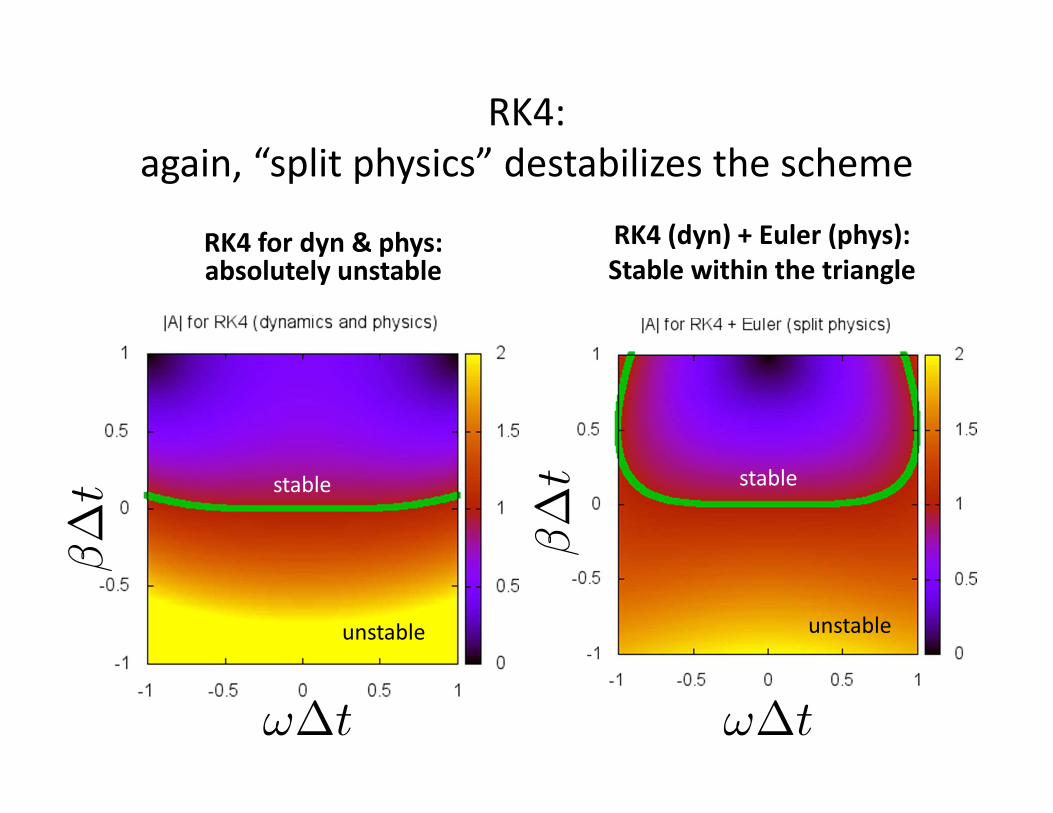
RK4:again, “split physics” destabilizes the scheme
unstable
stable
unstable
stable
RK4 for dyn & phys: absolutely unstable
RK4 (dyn) + Euler (phys): Stable within the triangle

Summary
• For leapfrog, doing “split physics” works very well (stabilizes the scheme)
• However, for Lorenz 4‐cycle (and equivalently, for RK4), “split physics” acts to destabilized the scheme.
• The latter is consistent with what I found by doing “split physics” with SPEEDY model.

The Bug (1)
Leapfrog (default)PROGRAM agcmCALL iniall ()IDAY=0; CALL FORDATE()CALL STEPONE() ! 1st step by Euler ForwardDO ! loop over a monthDO ! loop over a dayCALL FORDATE()CALL STLOOP() ! integrate for a dayEND DO
END DO
N‐cycle (with bug)PROGRAM agcmCALL iniall ()
DO ! loop over a monthDO ! loop over a dayCALL FORDATE()CALL STLOOP() ! integrate for a dayEND DO
END DO

The Bug (2)
N‐cycle (fixed)PROGRAM agcmCALL iniall ()IDAY=0; CALL FORDATE()
DO ! loop over a monthDO ! loop over a dayCALL FORDATE()CALL STLOOP() ! integrate for a dayEND DO
END DO
N‐cycle (with bug)PROGRAM agcmCALL iniall ()
DO ! loop over a monthDO ! loop over a dayCALL FORDATE()CALL STLOOP() ! integrate for a dayEND DO
END DO
Recommended