Recognize basic emotional statesin speech by machine learning techniques using mel-frequency cepstral coefficient features
Article
Accepted Version
Yang, N., Dey, N., Sherratt, R. S. and Shi, F. (2020) Recognize basic emotional statesin speech by machine learning techniques using mel-frequency cepstral coefficient features. Journal of Intelligent & Fuzzy Systems, 39 (2). pp. 1925-1936. ISSN 1875-8967 doi: https://doi.org/10.3233/JIFS-179963 Available at http://centaur.reading.ac.uk/88046/
It is advisable to refer to the publisher’s version if you intend to cite from the work. See Guidance on citing .
To link to this article DOI: http://dx.doi.org/10.3233/JIFS-179963
Publisher: IOS Press
Publisher statement: Special issue: Applied Machine Learning & Management of Volatility, Uncertainty, Complexity and Ambiguity

All outputs in CentAUR are protected by Intellectual Property Rights law, including copyright law. Copyright and IPR is retained by the creators or other copyright holders. Terms and conditions for use of this material are defined in the End User Agreement .
www.reading.ac.uk/centaur
CentAUR
Central Archive at the University of Reading
Reading’s research outputs online
Emotional State Recognition for AI Smart
Home Assistants using Mel-Frequency
Cepstral Coefficient Features
Ningning Yanga, Nilanjan Deyb, R. Simon Sherrattc and Fuqian Shia,*
aFirst Affiliated Hospital of Wenzhou Medical University, Wenzhou 325035, China; [email protected] bDepartment of Information Technology, Techno India College of Technology, West Bengal 740000, India;
[email protected] c Department of Biomedical Engineering, the University of Reading, RG6 6AY, UK; [email protected]
Abstract. AI based Speech Recognition has been widely used in the consumer field for control of smart home personal assistants,
with many such devices on the market. Smart home assistants that could detect the user’s emotion would improve the
communication between a user and the assistant enabling the assistant to offer more productive feedback. Thus, the aim of this
work is to analyze emotional states in speech and propose a suitable algorithm considering performance verses complexity for
deployment in smart home devices. The four emotional speeches were selected from the Berlin Emotional Database (EMO-DB)
as experimental data, 26 MFCC features were extracted from each type of emotional speech to identify the emotions of happiness,
anger, sadness and neutrality. Then, speaker-independent experiments for our Speech emotion Recognition (SER) were
conducted by using the Back Propagation Neural Network (BPNN), Extreme Learning Machine (ELM), Probabilistic Neural
Network (PNN) and Support Vector Machine (SVM). Synthesizing the recognition accuracy and processing time, this work
shows that the performance of SVM was the best among the four methods as a good candidate to be deployed for SER in smart
home devices. SVM achieved an overall accuracy of 92.4% while offering low computational requirements when training and
testing. We conclude that the MFCC features and the SVM classification models used in speaker-independent experiments are
highly effective in the automatic prediction of emotion.
Keywords: Emotion recognition, back propagation neural network, extreme learning machine, Mel-frequency cepstral
coefficients, smart home, support vector machine
1. Introduction
Speech Emotion Recognition (SER) was first
proposed in 1997 by Picard [1] and has attracted
widespread attention. It is well known that language
communication is the preferred method when
communicating with others in daily life, and human
language is first formed through speech. It can be said
that speech plays a decisive supporting role in
language. Human speech not only contains important
semantic information, but also implies rich emotional
information [2]. The aim of SER is to obtain the
emotional states of a user derived from their speech
*Corresponding author. E-mail: [email protected]
[3], thereby achieving harmonious communication
between humans or between humans and machines.
Emotion is a comprehensive state that occurs when
an individual receives an internal or external stimulus,
including physiological reaction, subjective
experience and external behavior [4]. When the
internal or external stimulus are consistent with a
user's needs or requests, they will experience positive
emotions, whereas negative emotions can be
experienced with unpleasant experiences or distress.
The ability for consumer devices to detect emotion
has been a hot research topic since 2006 with the
introduction of an early music recommender system
[5], and facial expression recognition [6] for personal
cameras in 2010. The first emotion recognition
systems in the consumer field appeared in 2011 that
used a database [7], and then biofeedback [8]. While
research into music recommender systems has been
buoyant [9,10], other interesting systems for human
emotion include lighting for emotion [11] and emotion
aware service robots [12], [13]. Recent research
indicates seamless human-device interaction [14].
With the advent of smart consumer home devices [15],
consumers can live in their home for longer, safer [16]
and to live healthier lifestyles [17].
McNally [18] presented six basic emotions - anger,
disgust, fear, happiness, sadness, surprise, and these
are widely used in current research. Emotion can be
roughly divided into two forms: discrete and
dimensional [19]. Discrete emotion description
utilizes fixed labels to describe emotions, such as
happiness, anger and sadness. The dimensional
emotion description describes emotional attributes
with points in multi-dimensional space, such as the
arousal-valence model in two dimensions [20,21], the
position – arousal–dominance model in three
dimensions [22] and the Hevner emotion ring model
[23]. The two emotion description methods have their
own advantages. Discrete emotion description has
been widely used for SER with its advantages of being
simple and easy to understand. At present, the acoustic
features have been widely applied to study SER, and
many remarkable achievements have been made
[24,25].
The emotional features based on acoustics can be
roughly classified into three types: prosodic features,
spectral features and sound quality features [26]. The
prosodic features [27] can reflect the changes of
intensity and intonation in speech. The commonly
used prosodic features have duration, pitch and energy.
The spectral features may be divided into linear
spectral features and cepstral features. The linear
spectral features include the linear predictor
coefficient (LPC) and the log-frequency power
coefficient (LFPC). The cepstral features [28] include
the Mel-Frequency Cepstral Coefficient (MFCC) and
the linear predictor cepstral coefficient (LPCC).
Among them, the MFCC is the most commonly used
spectral feature for SER because of its characteristics
being similar to the human ear. Sound quality features
have a great influence on the emotional state
expressed in speech, and it mainly includes sounds
from breathing, brightness and formant [29]. Acoustic
features are typically extracted in frames and enable
emotional recognition through simple statistical
analysis.
The rapid development of SER cannot be separated
from the support of computer technology. Advanced
computer technology has laid a solid foundation for
the development of SER [30]. The task of SER is to
extract the characteristic parameters that can reflect
emotions from speech signals and then find out the
mapping relationship between these characteristic
parameters and human emotions [31].
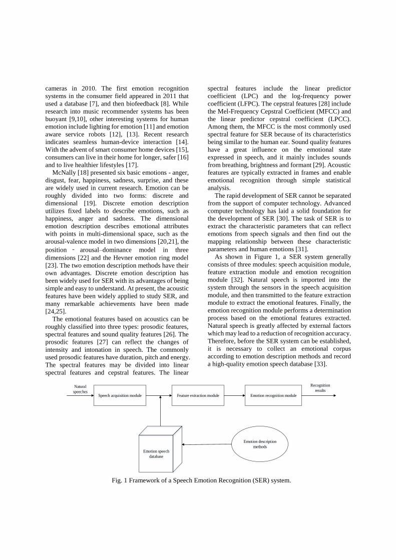
As shown in Figure 1, a SER system generally
consists of three modules: speech acquisition module,
feature extraction module and emotion recognition
module [32]. Natural speech is imported into the
system through the sensors in the speech acquisition
module, and then transmitted to the feature extraction
module to extract the emotional features. Finally, the
emotion recognition module performs a determination
process based on the emotional features extracted.
Natural speech is greatly affected by external factors
which may lead to a reduction of recognition accuracy.
Therefore, before the SER system can be established,
it is necessary to collect an emotional corpus
according to emotion description methods and record
a high-quality emotion speech database [33].
Fig. 1 Framework of a Speech Emotion Recognition (SER) system.
Speech acquisition module Feature extraction module Emotion recognition module
Recognition
resultsNatural
speeches
Emotion speech
database
Emotion description
methods
SER is essentially a pattern recognition problem; it
can be realized through using the standard pattern
classifiers [34]. At present, the classifiers commonly
used for SER are: Artificial Neural Network (ANN),
Support Vector Machine (SVM), Hidden Markov
Model (HMM) and Gaussian Mixture Model (GMM).
Rajisha et al. [39] extracted MFCCs, energy and pitch
as emotional features and performed emotional
recognition on the Malayalam emotion database using
ANN and SVM as classifiers. The experimental
results showed a classification accuracy of 88.4% for
ANN and the classification accuracy of 78.2% for
SVM. Sujatha and Ameena [40] conducted speaker-
independent and speaker-dependent emotional
recognition on the IITKGP-SESC and IITKGP-
SEHSC databases. The recognition results using
GMM, HMM and SVM as classifiers were that the
recognition for seven different emotions in the
speaker-dependent case was better than the speaker-
independent case. In the speaker-independent case,
GMM performed better on anger and surprise
emotions and HMM performed better on disgust, fear
and neutrality emotions. SVM achieved an average
recognition accuracy of 86.6% for test samples of an
unknown emotion. Lanjewar et al. [41] used GMM
and K-Nearest Neighbor (KNN) as classifiers to
identify six emotions in speech (including happiness,
anger, sadness, fear, surprise and neutrality) using the
Berlin Emotional Database (EMO-DB) [42]. GMM
was more effective on the anger emotion with a 92%
recognition rate while KNN achieved the highest
recognition rate of 90% on happiness emotion.
Although many classifiers can be applied to identify
emotions in speech, each classifier has its own
advantages and disadvantages, so the appropriate
classification model needs to be selected according to
the requirements.
This paper is concerned with defining suitable
technology to enable smart home assistants, as a voice
sensor, to predict the emotional state of a user, and in
doing so offer more suitable responses to questions
and home events. The work considers many classifiers
and has found that the Support Vector Machine
(SVM) is an excellent candidate for SER when
considering both recognition performance, and real-
time operation.
The rest of the article is structured as follows: The
specific process to perform SER will be provided in
Section II. Section III will introduce the testing
methodology in detail. The experimental results and
relevant discussion are presented in Section IV.
Finally, conclusion and future works will be given in
Section V.
2. Materials and Methods
In a practical system deployment, real-time user
speech would be used. However, in order to compare
and validate with other works, the EMO-DB database
[42] has been used. The specific process of performing
SER in this work is shown in Figure 2. The emotional
speech selected from the database is first preprocessed
to reduce noise interference and keep information
integrity [43]. Then, extraction of emotional features
is performed. The extracted data is then divided into
training data and test data. The training data is used to
train models and obtain classification rules whereas
the test data is determined to belong to which type of
emotions based on classification rules obtained from
the training data. Finally, the recognition results are
outputted. In this section, each step of SER is
described in detail.
2.1. Emotion speech database
The EMO-DB database contains seven emotions:
happiness, anger, sadness, neutrality, fear, disgust and
boredom [44]. It was created using five male and five
female actors who simulated emotions on five long
sentences and five short sentences. Finally, the 535
speech recordings are retained after listening
experiments of 10 males and 10 females with the
length of each speech being 3~8s. The EMO-DB
database was stored at a sampling rate of 16 kHz 16-
bit quantization and stored in the common .wav file
format.
2.2. Speech preprocessing
The purpose of preprocessing is to highlight the
emotional information and reduce the impact of other
information. The speech signal is a non-stationery and
time-varying signal [45], but its characteristics remain
basically unchanged in a short time range (generally
considered to be 10-30ms), i.e. speech has short-term
stability. Therefore, most systems adopt framing to
preprocess speech [39]. Generally, the frame length is
10 to 30ms.
Before extracting emotional features, this work has
used the Music Analysis, Retrieval and Synthesis for
Audio Signals (MARSYAS) tool [46] to automatically
frame speech, and its parameters are set as shown in
Table 1.
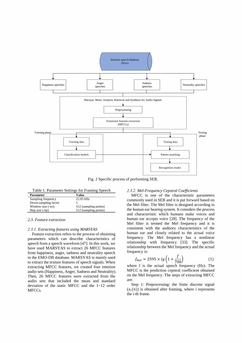
Table 1. Parameter Settings for Framing Speech Parameter Value
Sampling frequency 22.05 kHz
Down-sampling factor 1
Window size (-ws) 512 (sampling points) Hop size (-hp) 512 (sampling points)
2.3. Feature extraction
2.3.1. Extracting features using MARSYAS
Feature extraction refers to the process of obtaining
parameters which can describe characteristics of
speech from a speech waveform [47]. In this work, we
have used MARSYAS to extract 26 MFCC features
from happiness, anger, sadness and neutrality speech
in the EMO-DB database. MARSYAS is mainly used
to extract the texture features of speech signals. When
extracting MFCC features, we created four emotion
audio sets (Happiness, Anger, Sadness and Neutrality).
Then, 26 MFCC features were extracted from the
audio sets that included the mean and standard
deviation of the static MFCC and the 1~12 order
MFCCs.
2.3.2. Mel-Frequency Cepstral Coefficients
MFCC is one of the characteristic parameters
commonly used in SER and it is put forward based on
the Mel filter. The Mel filter is designed according to
the human ear hearing system. It considers the process
and characteristic which humans make voices and
human ear accepts voice [28]. The frequency of the
Mel filter is termed the Mel frequency and it is
consistent with the auditory characteristics of the
human ear and closely related to the actual voice
frequency. The Mel frequency has a nonlinear
relationship with frequency [33]. The specific
relationship between the Mel frequency and the actual
frequency is:
𝑓𝑀𝑒𝑙 = 2595 × 𝑙𝑔 (1 +𝑓
700) (1)
where f is the actual speech frequency (Hz). The
MFCC is the prediction cepstral coefficient obtained
on the Mel frequency. The steps of extracting MFCC
are:
Step 1: Preprocessing: the finite discrete signal
(𝑥𝑖(𝑛)) is obtained after framing, where i represents
the i-th frame.
Fig. 2 Specific process of performing SER.
Emotion speech database
(Wav)
Happiness speechesAnger
speeches
Sadness
speechesNeutrality speeches
Preprocessing
Emotional features extraction
(MFCCs)
Marsyas: Music Analysis, Retrieval and Synthesis for Audio Signals
Training data Testing data
Classification models Pattern matching
Recognition results
Training phase Testing
phase
Step 2: The Fast Fourier Transform (FFT) is applied
to each frame:
𝑋(𝑖, 𝑘) = 𝐹𝐹𝑇[𝑥𝑖(𝑛)] = ∑ 𝑥𝑖(𝑛)𝑊𝑁𝑘𝑛
𝑁−1
𝑛=0
𝑘 = 0,1, … , 𝑁 − 1 (2) where N is the number of sampling points in each
frame. Then the power spectrum is obtained:
𝐸(𝑖, 𝑘) = [𝑋(𝑖, 𝑘)]2 (3) Step 3: Calculate the energy through the Mel filter.
𝑆(𝑖, 𝑚) = ∑ 𝐸(𝑖, 𝑘)𝐻𝑚(𝑘)
𝑁−1
𝑘=0
(4)
Step 4: Calculate MFCC using the Discrete Cosine
Transform (DCT).
𝑀𝐹𝐶𝐶(𝑖, 𝑛)
= √2
𝑀∑ 𝑙𝑜𝑔[𝑆(𝑖, 𝑚)] 𝑐𝑜𝑠 (
𝜋𝑛(𝑚 − 0.5)
𝑀)
𝑀−1
𝑚=0
𝑛 = 1,2, … , 𝐿 (5)
where n represents the order of the MFCC, and L is
usually taken as 12. M is the number of Mel filters.
2.4. Classification model
2.4.1. Back Propagation Neural Network (BPNN)
BPNN is a multi-layer feedforward neural network
[48] famous for being a back propagation (BP)
algorithm. The BPNN algorithm includes two
processes: forward transmission of signals and back
propagation of errors [49]. In the forward transmission
speech signals are transmitted from the input layer
through the hidden layer to calculate the outputs of
output layer. In back propagation of errors, the output
error of network is first calculated as:
𝐸 = 1
2 ∑(𝑇𝑘 − 𝑂𝑘)2
𝐿
𝑘=1
𝑘 = 1,2, … , 𝑚 (6)
where 𝑇𝑘 and 𝑂𝑘 represent the expected output and
the actual output of the k-th node in the output layer
respectively. Then, according to the gradient descent
algorithm Error! Reference source not found., the
adjustment formula for the weights ( 𝑤𝑘𝑖&𝑤𝑖𝑗 ) and
thresholds (𝑎𝑘&𝜃𝑖) are obtained:
𝑤𝑘𝑖 = 𝑤𝑘𝑖 + ∆𝑤𝑘𝑖 = 𝑤𝑘𝑖 − 𝜂𝜕𝐸
𝜕𝑤𝑘𝑖
(7)
𝑎𝑘 = 𝑎𝑘 + ∆𝑎𝑘 = 𝑎𝑘 − 𝜂𝜕𝐸
𝜕𝑎𝑘
(8)
𝑤𝑖𝑗 = 𝑤𝑖𝑗 + ∆𝑤𝑖𝑗 = 𝑤𝑖𝑗 − 𝜂𝜕𝐸
𝜕𝑤𝑖𝑗
(9)
𝜃𝑖 = 𝜃𝑖 + ∆𝜃𝑖 = 𝜃𝑖 − 𝜂𝜕𝐸
𝜕𝜃𝑖
(10)
where 𝑤𝑘𝑖 represents the weight between the k-th
node in the output layer and the i-th node in the hidden
layer, 𝑎𝑘 represents the threshold of the k-th node in
the output layer, 𝑤𝑖𝑗 represents the weight between
the i-th node in the hidden layer and the j-th node in
the input layer, 𝜃𝑖 represents the threshold of the i-th
node in the hidden layer and 𝜂 represents the learning
rate.
2.4.2. Extreme Learning Machine (ELM)
ELM was proposed in 2004 by Huang [51].
Different from traditional algorithms (such as BP
algorithm), ELM randomly generates the weights
between the input layer, the hidden layer, and the
thresholds of the hidden layer node. The thresholds do
not need to be adjusted during the training process. It
only needs to set the number of nodes in the hidden
layer to determine the weights between the hidden
layer and the output layer by solving the equation set
[52].
Let the number of neurons in the input layer, hidden
layer and output layer be n, l and m respectively, the
weight matrix between the hidden layer and the input
layer is 𝒘 = [𝑤𝑖𝑗]𝑙×𝑛, the weight matrix between the
hidden layer and the output layer is 𝜷 = [𝛽𝑖𝑘]𝒍×𝒎, the
threshold matrix of the hidden layer is 𝒃 = [𝑏𝑖]𝑙×1, the
input sample is 𝒙 = [𝑥𝑗]𝑛×1 , and the activation
function of the hidden layer is 𝑔(𝑥), then the actual
output matrix of the output layer (𝑶 = [𝑂𝑘]𝑚×1) can
be expressed by:
𝑯𝜷 = 𝑶𝑻 (11)
where 𝑯 = [𝑔(𝒘𝑖𝐱 + 𝒃𝒊)]𝟏×𝒍 is the output matrix of
the hidden layer, 𝒘𝑖 represents the i-th row of matrix
𝒘; 𝑶𝑻 is the transpose of the matrix 𝑶. The ELM
optimization not only minimizes the network error,
but also minimizes the weights between the hidden
layer and the output layer. Therefore, the optimization
objective equation is:
𝑚𝑖𝑛𝛽
∥ 𝑯𝜷 − 𝑻𝑻 ∥ (12)
where 𝑻 = [𝑇𝑘]𝑚×1 is the expected output matrix of
the output layer, 𝑻𝑻 is the transpose of the matrix 𝑻.
Finally, the weights of between the hidden layer and
the output layer is given by:
�̂� = 𝑯+𝑻𝑻 (13)
where 𝑯+ is the Moore-Penrose generalized inverse
of matrix H.
2.4.3. Probabilistic Neural Network (PNN)
The theoretical basis of PNN is the Bayesian
decision theory and Parzen probability density
estimation [53]. During training, PNN does not need
error back propagation like BPNN as it only contains
a forward calculation process [54]. PNN consists of an
input layer, pattern layer, accumulation layer and
output layer. The first layer is the input layer
responsible for transmitting the feature vectors in the
training samples to the network. The number of
neurons in this layer is equal to the dimension of the
feature vector. The second layer is the pattern layer, its
function is to calculate the matching relationship
between the feature vector and each category, and the
number of neurons in this layer is same with the sum
of training samples. The output of the j-th neuron of
the i-th category in the pattern layer is:
𝜙𝑖𝑗(𝒙) =1
(2𝜋)12𝜎𝑑
𝑒𝑥 𝑝 [−(𝒙 − 𝒄𝒊𝒋)(𝒙 − 𝒄𝒊𝒋)
𝑇
𝜎2]
𝑖 = 1,2, … , 𝑀; 𝑗 = 1,2, … , 𝐿𝑖 (14)
where 𝒙 represents the input vector with d as its
dimension, 𝒄𝒊𝒋 represents the center of the j-th
neuron of the i-th category in the pattern layer, M is
the number of categories in the training samples, 𝐿𝑖
is the number of neurons of the i-th category in the
pattern layer, 𝜎 is the smoothing factor, it plays an
important role in network performance.
The third layer is the accumulation layer, it
accumulates the probability density function of each
category according to:
𝑣𝑖 =1
𝐿𝑖
∑ 𝜙𝑖𝑗
𝐿𝑖
𝑗=1
(15)
where 𝑣𝑖 represents the output of the i-th category.
The number of neurons in the accumulation layer is
equal to M. Finally, the adjudicative result is output by
the output layer. There is only one ‘1’ in the output
result and the rest are ‘0’. The output of the class with
the largest probability density function is 1, that is:
𝑦 = 𝑎𝑟𝑔𝑚𝑎𝑥(𝑣𝑖) (16)
2.4.4. Support Vector Machine (SVM)
SVM is a supervised machine learning method
based on statistical learning theory and structural risk
minimization [55]. The basic idea of SVM is - for the
nonlinear and separable problem of the input space,
the input vector is mapped to the high-dimensional
feature space through selecting the appropriate kernel
function. Then, the optimal separating hyperplane is
constructed in the high-dimensional feature space to
make the corresponding sample space linearly
separable [56]. The objective function corresponding
to the nonlinear separable SVM is:
{𝑚𝑖𝑛 (
1
2𝒘𝑇𝒘 + 𝐶 ∑ 𝜉𝑖
𝑁
𝑖=1
)
𝑠. 𝑡. 𝒀𝑖(𝒘𝑇𝑿𝑖 + 𝑏) + 𝜉𝑖 ≥ 1
𝜉𝑖 > 0, 𝑖 = 1,2, … , 𝑁 (17)
where {𝑿𝑖 , 𝒀𝑖} represents the training sample set, 𝑿𝑖
is the n dimensional feature vector, 𝒀𝑖 ∈ {−1,1}
represents the sample category, N represents the
number of the training samples, w is the weight vector,
b is the classification threshold, 𝑠. 𝑡. represents the
constraint condition, C is the penalty coefficient, it
controls the degree of punishment for the wrong
classification samples and it has the effect of
balancing complexity and loss error of the model, 𝜉𝑖
is the relaxation factor which is used to control the
classification surface to allow the existence of the
wrong classification samples in classifying.
The input vectors 𝑿𝑖 and 𝑿𝑗 adopt the mapping
function 𝝓(∙) from the data space to the feature space,
and the kernel function transformation equation
(𝑿𝑖 , 𝑿𝑗) → K(𝑿𝑖 , 𝑿𝑗) = 𝝓(𝑿𝑖) ∙ 𝝓(𝑿𝑗) to get the
optimal hyperplane function:
𝑓(𝑥) = 𝑠𝑔𝑛 [∑ 𝛼𝑖𝒀𝑖𝐾(𝑿𝑖 , 𝑿)
𝑁
𝑖=1
+ 𝑏] (18)
where 𝛼𝑖 is the Lagrangian multiplier and 𝑠𝑔𝑛(∙) is
the sign function. Finally, the classification results are
output according to the optimal hyperplane function.
The SVM algorithm is originally designed for
binary classification. When dealing with multi-
classification problems, it is necessary to construct a
suitable multi-classification SVM. The common
method for constructing multi-classification SVM is
the one-to-one method, it is to design a SVM between
any two classes, which can convert c-class
classification patterns into 𝑐(𝑐 − 1)/2 two-class
classification patterns [57]. The four emotions of
happiness, anger, sadness and neutrality in speech are
classified, so six SVMs need to be built. Each SVM is
used to identify any two emotions of the four emotions,
namely happiness-anger, happiness-sadness,
happiness-neutrality, anger-sadness, anger-neutrality
and sadness-neutrality. When classifying an unknown
sample, the six SVMs discriminate it, and finally the
emotional category with the highest win frequency is
taken as the emotion of the unknown sample. The win
frequency for each class refers to the ratio between the
number which the unknown sample is divided into this
class and the total number which the unknown sample
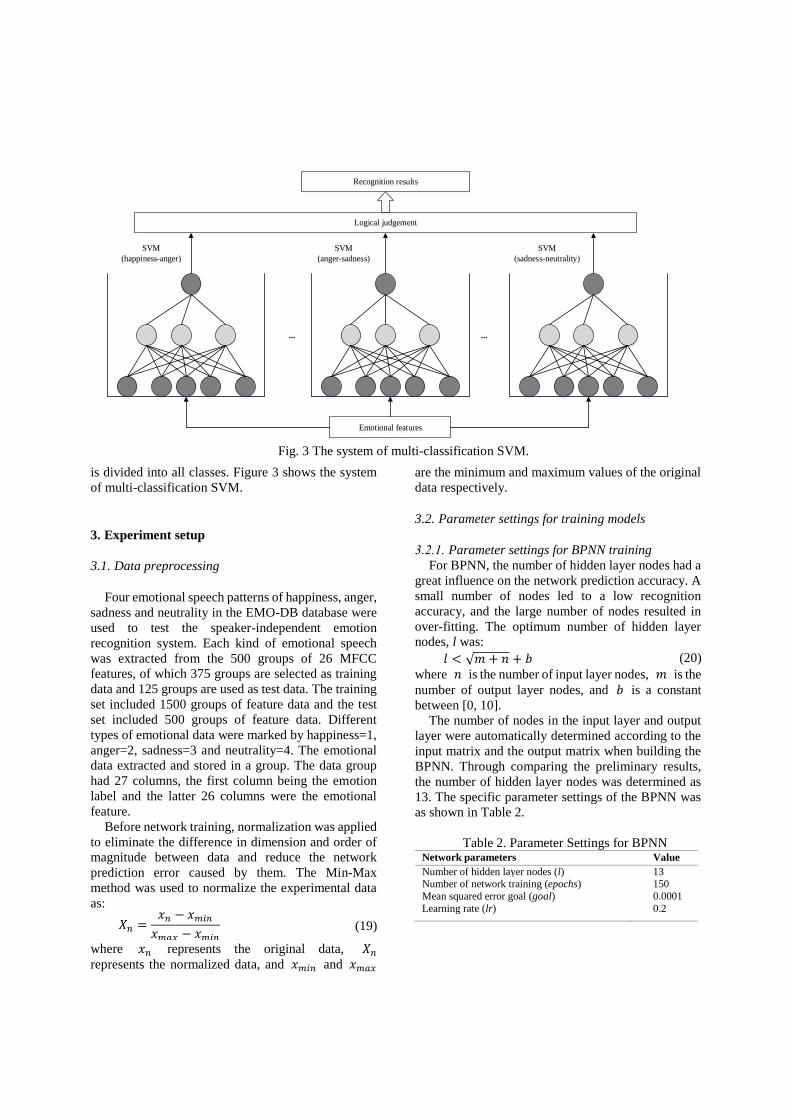
is divided into all classes. Figure 3 shows the system
of multi-classification SVM.
3. Experiment setup
3.1. Data preprocessing
Four emotional speech patterns of happiness, anger,
sadness and neutrality in the EMO-DB database were
used to test the speaker-independent emotion
recognition system. Each kind of emotional speech
was extracted from the 500 groups of 26 MFCC
features, of which 375 groups are selected as training
data and 125 groups are used as test data. The training
set included 1500 groups of feature data and the test
set included 500 groups of feature data. Different
types of emotional data were marked by happiness=1,
anger=2, sadness=3 and neutrality=4. The emotional
data extracted and stored in a group. The data group
had 27 columns, the first column being the emotion
label and the latter 26 columns were the emotional
feature.
Before network training, normalization was applied
to eliminate the difference in dimension and order of
magnitude between data and reduce the network
prediction error caused by them. The Min-Max
method was used to normalize the experimental data
as:
𝑋𝑛 =𝑥𝑛 − 𝑥𝑚𝑖𝑛
𝑥𝑚𝑎𝑥 − 𝑥𝑚𝑖𝑛
(19)
where 𝑥𝑛 represents the original data, 𝑋𝑛
represents the normalized data, and 𝑥𝑚𝑖𝑛 and 𝑥𝑚𝑎𝑥
are the minimum and maximum values of the original
data respectively.
3.2. Parameter settings for training models
3.2.1. Parameter settings for BPNN training
For BPNN, the number of hidden layer nodes had a
great influence on the network prediction accuracy. A
small number of nodes led to a low recognition
accuracy, and the large number of nodes resulted in
over-fitting. The optimum number of hidden layer
nodes, l was:
𝑙 < √𝑚 + 𝑛 + 𝑏 (20)
where 𝑛 is the number of input layer nodes, 𝑚 is the
number of output layer nodes, and 𝑏 is a constant
between [0, 10].
The number of nodes in the input layer and output
layer were automatically determined according to the
input matrix and the output matrix when building the
BPNN. Through comparing the preliminary results,
the number of hidden layer nodes was determined as
13. The specific parameter settings of the BPNN was
as shown in Table 2.
Table 2. Parameter Settings for BPNN Network parameters Value
Number of hidden layer nodes (l) 13 Number of network training (epochs) 150
Mean squared error goal (goal) 0.0001
Learning rate (lr) 0.2
Fig. 3 The system of multi-classification SVM.
Emotional features
... ...
Logical judgement
Recognition results
SVM
(happiness-anger)
SVM
(anger-sadness)
SVM
(sadness-neutrality)
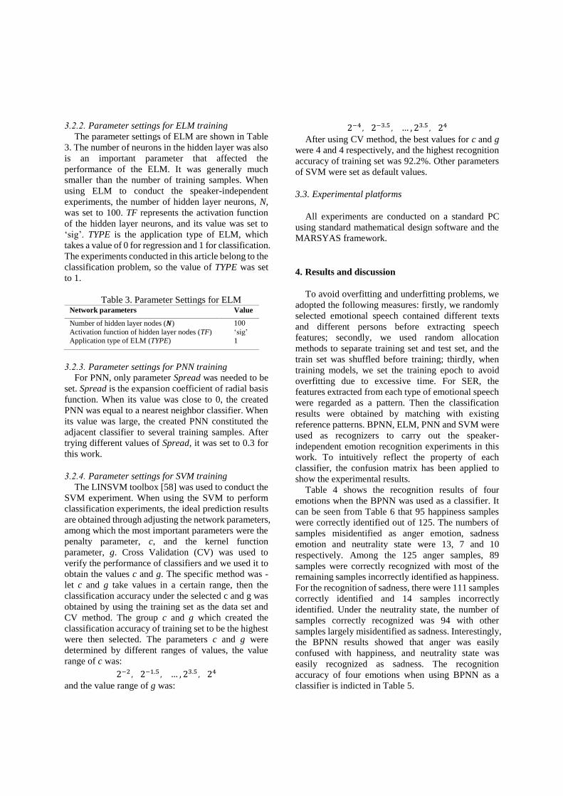
3.2.2. Parameter settings for ELM training
The parameter settings of ELM are shown in Table
3. The number of neurons in the hidden layer was also
is an important parameter that affected the
performance of the ELM. It was generally much
smaller than the number of training samples. When
using ELM to conduct the speaker-independent
experiments, the number of hidden layer neurons, N,
was set to 100. TF represents the activation function
of the hidden layer neurons, and its value was set to
‘sig’. TYPE is the application type of ELM, which
takes a value of 0 for regression and 1 for classification.
The experiments conducted in this article belong to the
classification problem, so the value of TYPE was set
to 1.
Table 3. Parameter Settings for ELM Network parameters Value
Number of hidden layer nodes (𝑵) 100
Activation function of hidden layer nodes (TF) ‘sig’ Application type of ELM (TYPE) 1
3.2.3. Parameter settings for PNN training
For PNN, only parameter Spread was needed to be
set. Spread is the expansion coefficient of radial basis
function. When its value was close to 0, the created
PNN was equal to a nearest neighbor classifier. When
its value was large, the created PNN constituted the
adjacent classifier to several training samples. After
trying different values of Spread, it was set to 0.3 for
this work.
3.2.4. Parameter settings for SVM training
The LINSVM toolbox [58] was used to conduct the
SVM experiment. When using the SVM to perform
classification experiments, the ideal prediction results
are obtained through adjusting the network parameters,
among which the most important parameters were the
penalty parameter, c, and the kernel function
parameter, g. Cross Validation (CV) was used to
verify the performance of classifiers and we used it to
obtain the values c and g. The specific method was -
let c and g take values in a certain range, then the
classification accuracy under the selected c and g was
obtained by using the training set as the data set and
CV method. The group c and g which created the
classification accuracy of training set to be the highest
were then selected. The parameters c and g were
determined by different ranges of values, the value
range of c was:
2−2,2−1.5,… , 23.5,24
and the value range of g was:
2−4,2−3.5,… , 23.5,24
After using CV method, the best values for c and g
were 4 and 4 respectively, and the highest recognition
accuracy of training set was 92.2%. Other parameters
of SVM were set as default values.
3.3. Experimental platforms
All experiments are conducted on a standard PC
using standard mathematical design software and the
MARSYAS framework.
4. Results and discussion
To avoid overfitting and underfitting problems, we
adopted the following measures: firstly, we randomly
selected emotional speech contained different texts
and different persons before extracting speech
features; secondly, we used random allocation
methods to separate training set and test set, and the
train set was shuffled before training; thirdly, when
training models, we set the training epoch to avoid
overfitting due to excessive time. For SER, the
features extracted from each type of emotional speech
were regarded as a pattern. Then the classification
results were obtained by matching with existing
reference patterns. BPNN, ELM, PNN and SVM were
used as recognizers to carry out the speaker-
independent emotion recognition experiments in this
work. To intuitively reflect the property of each
classifier, the confusion matrix has been applied to
show the experimental results.
Table 4 shows the recognition results of four
emotions when the BPNN was used as a classifier. It
can be seen from Table 6 that 95 happiness samples
were correctly identified out of 125. The numbers of
samples misidentified as anger emotion, sadness
emotion and neutrality state were 13, 7 and 10
respectively. Among the 125 anger samples, 89
samples were correctly recognized with most of the
remaining samples incorrectly identified as happiness.
For the recognition of sadness, there were 111 samples
correctly identified and 14 samples incorrectly
identified. Under the neutrality state, the number of
samples correctly recognized was 94 with other
samples largely misidentified as sadness. Interestingly,
the BPNN results showed that anger was easily
confused with happiness, and neutrality state was
easily recognized as sadness. The recognition
accuracy of four emotions when using BPNN as a
classifier is indicted in Table 5.
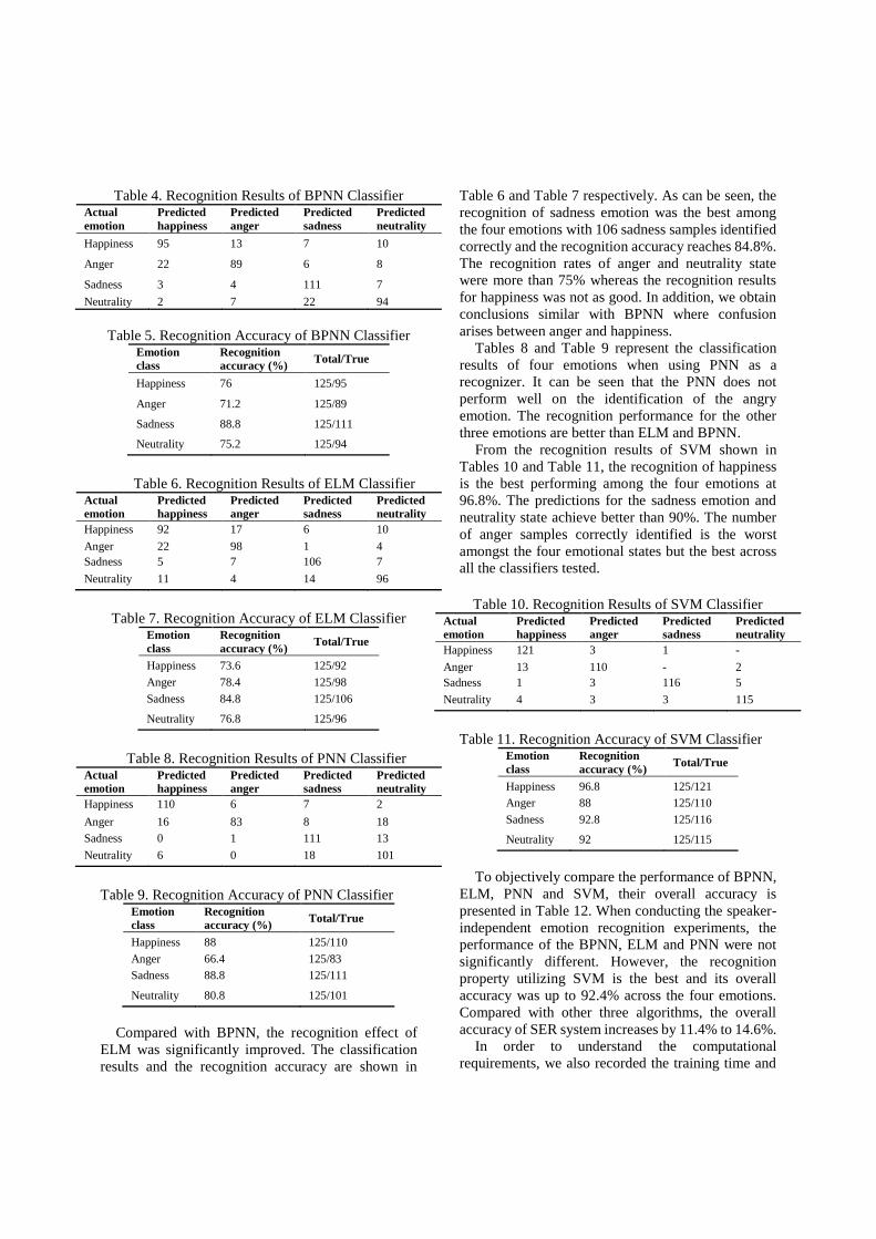
Table 4. Recognition Results of BPNN Classifier Actual
emotion
Predicted
happiness
Predicted
anger
Predicted
sadness
Predicted
neutrality
Happiness 95 13 7 10
Anger 22 89 6 8
Sadness 3 4 111 7
Neutrality 2 7 22 94
Table 5. Recognition Accuracy of BPNN Classifier Emotion
class
Recognition
accuracy (%) Total/True
Happiness 76 125/95
Anger 71.2 125/89
Sadness 88.8 125/111
Neutrality 75.2 125/94
Table 6. Recognition Results of ELM Classifier Actual
emotion
Predicted
happiness
Predicted
anger
Predicted
sadness
Predicted
neutrality
Happiness 92 17 6 10
Anger 22 98 1 4
Sadness 5 7 106 7
Neutrality 11 4 14 96
Table 7. Recognition Accuracy of ELM Classifier Emotion
class
Recognition
accuracy (%) Total/True
Happiness 73.6 125/92
Anger 78.4 125/98
Sadness 84.8 125/106
Neutrality 76.8 125/96
Table 8. Recognition Results of PNN Classifier Actual
emotion
Predicted
happiness
Predicted
anger
Predicted
sadness
Predicted
neutrality
Happiness 110 6 7 2
Anger 16 83 8 18
Sadness 0 1 111 13
Neutrality 6 0 18 101
Table 9. Recognition Accuracy of PNN Classifier Emotion
class
Recognition
accuracy (%) Total/True
Happiness 88 125/110
Anger 66.4 125/83
Sadness 88.8 125/111
Neutrality 80.8 125/101
Compared with BPNN, the recognition effect of
ELM was significantly improved. The classification
results and the recognition accuracy are shown in
Table 6 and Table 7 respectively. As can be seen, the
recognition of sadness emotion was the best among
the four emotions with 106 sadness samples identified
correctly and the recognition accuracy reaches 84.8%.
The recognition rates of anger and neutrality state
were more than 75% whereas the recognition results
for happiness was not as good. In addition, we obtain
conclusions similar with BPNN where confusion
arises between anger and happiness.
Tables 8 and Table 9 represent the classification
results of four emotions when using PNN as a
recognizer. It can be seen that the PNN does not
perform well on the identification of the angry
emotion. The recognition performance for the other
three emotions are better than ELM and BPNN.
From the recognition results of SVM shown in
Tables 10 and Table 11, the recognition of happiness
is the best performing among the four emotions at
96.8%. The predictions for the sadness emotion and
neutrality state achieve better than 90%. The number
of anger samples correctly identified is the worst
amongst the four emotional states but the best across
all the classifiers tested.
Table 10. Recognition Results of SVM Classifier Actual
emotion
Predicted
happiness
Predicted
anger
Predicted
sadness
Predicted
neutrality
Happiness 121 3 1 -
Anger 13 110 - 2
Sadness 1 3 116 5
Neutrality 4 3 3 115
Table 11. Recognition Accuracy of SVM Classifier Emotion
class
Recognition
accuracy (%) Total/True
Happiness 96.8 125/121
Anger 88 125/110
Sadness 92.8 125/116
Neutrality 92 125/115
To objectively compare the performance of BPNN,
ELM, PNN and SVM, their overall accuracy is
presented in Table 12. When conducting the speaker-
independent emotion recognition experiments, the
performance of the BPNN, ELM and PNN were not
significantly different. However, the recognition
property utilizing SVM is the best and its overall
accuracy was up to 92.4% across the four emotions.
Compared with other three algorithms, the overall
accuracy of SER system increases by 11.4% to 14.6%.
In order to understand the computational
requirements, we also recorded the training time and
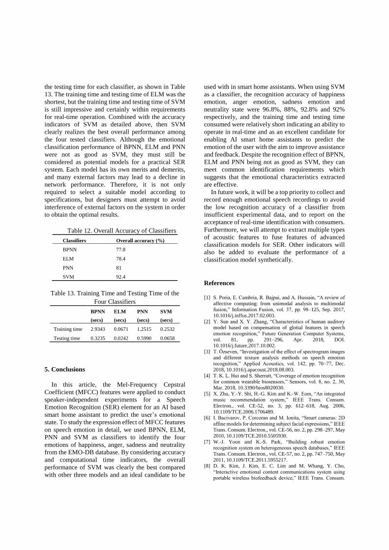
the testing time for each classifier, as shown in Table
13. The training time and testing time of ELM was the
shortest, but the training time and testing time of SVM
is still impressive and certainly within requirements
for real-time operation. Combined with the accuracy
indicators of SVM as detailed above, then SVM
clearly realizes the best overall performance among
the four tested classifiers. Although the emotional
classification performance of BPNN, ELM and PNN
were not as good as SVM, they must still be
considered as potential models for a practical SER
system. Each model has its own merits and demerits,
and many external factors may lead to a decline in
network performance. Therefore, it is not only
required to select a suitable model according to
specifications, but designers must attempt to avoid
interference of external factors on the system in order
to obtain the optimal results.
Table 12. Overall Accuracy of Classifiers
Classifiers Overall accuracy (%)
BPNN 77.8
ELM 78.4
PNN 81
SVM 92.4
Table 13. Training Time and Testing Time of the
Four Classifiers
BPNN
(secs)
ELM
(secs)
PNN
(secs)
SVM
(secs)
Training time 2.9343 0.0671 1.2515 0.2532
Testing time 0.3235 0.0242 0.5990 0.0658
5. Conclusions
In this article, the Mel-Frequency Cepstral
Coefficient (MFCC) features were applied to conduct
speaker-independent experiments for a Speech
Emotion Recognition (SER) element for an AI based
smart home assistant to predict the user’s emotional
state. To study the expression effect of MFCC features
on speech emotion in detail, we used BPNN, ELM,
PNN and SVM as classifiers to identify the four
emotions of happiness, anger, sadness and neutrality
from the EMO-DB database. By considering accuracy
and computational time indicators, the overall
performance of SVM was clearly the best compared
with other three models and an ideal candidate to be
used with in smart home assistants. When using SVM
as a classifier, the recognition accuracy of happiness
emotion, anger emotion, sadness emotion and
neutrality state were 96.8%, 88%, 92.8% and 92%
respectively, and the training time and testing time
consumed were relatively short indicating an ability to
operate in real-time and as an excellent candidate for
enabling AI smart home assistants to predict the
emotion of the user with the aim to improve assistance
and feedback. Despite the recognition effect of BPNN,
ELM and PNN being not as good as SVM, they can
meet common identification requirements which
suggests that the emotional characteristics extracted
are effective.
In future work, it will be a top priority to collect and
record enough emotional speech recordings to avoid
the low recognition accuracy of a classifier from
insufficient experimental data, and to report on the
acceptance of real-time identification with consumers.
Furthermore, we will attempt to extract multiple types
of acoustic features to fuse features of advanced
classification models for SER. Other indicators will
also be added to evaluate the performance of a
classification model synthetically.
References
[1] S. Poria, E. Cambria, R. Bajpai, and A. Hussain, “A review of
affective computing: from unimodal analysis to multimodal fusion,” Information Fusion, vol. 37, pp. 98–125, Sep. 2017,
10.1016/j.inffus.2017.02.003.
[2] Y. Sun and X. Y. Zhang, “Characteristics of human auditory model based on compensation of glottal features in speech
emotion recognition,” Future Generation Computer Systems,
vol. 81, pp. 291–296, Apr. 2018, DOI. 10.1016/j.future.2017.10.002.
[3] T. Özseven, “Investigation of the effect of spectrogram images
and different texture analysis methods on speech emotion recognition,” Applied Acoustics, vol. 142, pp. 70–77, Dec.
2018, 10.1016/j.apacoust.2018.08.003.
[4] T. K. L. Hui and S. Sherratt, “Coverage of emotion recognition for common wearable biosensors,” Sensors, vol. 8, no. 2, 30,
Mar. 2018, 10.3390/bios8020030.
[5] X. Zhu, Y.-Y. Shi, H.-G. Kim and K.-W. Eom, “An integrated music recommendation system,” IEEE Trans. Consum.
Electron., vol. CE-52, no. 3, pp. 612–618, Aug. 2006,
10.1109/TCE.2006.1706489. [6] I. Bacivarov, P. Corcoran and M. Ionita, “Smart cameras: 2D
affine models for determining subject facial expressions,” IEEE Trans. Consum. Electron., vol. CE-56, no. 2, pp. 298–297, May
2010, 10.1109/TCE.2010.5505930.
[7] W.-J. Yoon and K.-S. Park, “Building robust emotion recognition system on heterogeneous speech databases,” IEEE
Trans. Consum. Electron., vol. CE-57, no. 2, pp. 747–750, May
2011, 10.1109/TCE.2011.5955217. [8] D. K. Kim, J. Kim, E. C. Lim and M. Whang, Y. Cho,
“Interactive emotional content communications system using
portable wireless biofeedback device,” IEEE Trans. Consum.
Electron., vol. CE-57, no. 4, pp. 1929–1936, Nov. 2011,
10.1109/TCE.2011.6131173.
[9] K. Yoon, J. Lee and M.-U. Kim, “Music recommendation system using emotion triggering low-level features,” IEEE
Trans. Consum. Electron., vol. CE-58, no. 2, pp. 612–618, May
2012, 10.1109/TCE.2012.6227467. [10] R. L. Rosa, D. Z. Rodriguez and G. Bressan, “Music
recommendation system based on user's sentiments extracted
from social networks,” IEEE Trans. Consum. Electron., vol. CE-61, no. 3, pp. 359–367, Aug. 2015,
10.1109/TCE.2015.7298296.
[11] D. K. Kim, S. Ahn, S. Park and M. Whang, “Interactive emotional lighting system using physiological signals,” IEEE
Trans. Consum. Electron., vol. CE-59, no. 4, pp. 765–771, Nov.
2013, 10.1109/TCE.2013.6689687.
[12] J.-S. Park, J.-H. Kim and Y.-H. Oh, “Feature vector
classification-based speech emotion recognition for service
robots,” IEEE Trans. Consum. Electron., vol. CE-55, no. 3, pp. 1590–1596, Aug. 2009, 10.1109/TCE.2009.5278031.
[13] D.-S. Kim, S.-S. Lee and B.-H. Chol, “A real-time stereo depth
extraction hardware for intelligent home assistant robot,” IEEE Trans. Consum. Electron., vol. CE-56, no. 3, pp. 1782–1788,
Aug. 2010, 10.1109/TCE.2010.5606326.
[14] E. Rubio-Drosdov, D. Diaz-Sanchez, F. Almenarez, P. Arias-Cabarcos and A. Marin, “Seamless human-device interaction in
the internet of things,” IEEE Trans. Consum. Electron., vol. CE-63, no. 4, pp. 490–498, Nov. 2017,
10.1109/TCE.2017.015076.
[15] T. Perumal, A. R. Ramli and C. Y. Leong, “Design and implementation of SOAP-based residential management for
smart home systems,” IEEE Trans. Consum. Electron., vol. CE-
54, no. 2, pp. 453–459, May 2008, 10.1109/TCE.2008.4560114. [16] J. Wang, Z. Zhang, B. Li, S. Lee and R. S. Sherratt, “An
enhanced fall detection system for elderly person monitoring
using consumer home networks,” IEEE Trans. Consum. Electron., vol. CE-60, no. 1, pp. 23–29, Feb. 2014,
10.1109/TCE.2014.6780921.
[17] N Dey, A. S. Ashour, F. Shi, S. J. Fong and R. S. Sherratt, “Developing residential wireless sensor networks for ECG
healthcare monitoring,” IEEE Trans. Consum. Electron., vol.
CE-63, no. 4, pp. 442–449, Nov. 2017, 10.1109/TCE.2017.015063.
[18] R. J. McNally, “Handbook of cognition and emotion,” British
J. Psychiatry, vol. 176, no. 5, Jan. 1999, 10.1002/0470013494. [19] S. Hamann, “Mapping discrete and dimensional emotions onto
the brain: controversies and consensus,” Trends in Cognitive
Sciences, vol. 16, no. 9, pp. 458–466, Sep. 2012, 10.1016/j.tics.2012.07.006.
[20] C. Chih-Hao, L. Wei-Po, and H. Jhih-Yuan, “Tracking and
recognizing emotions in short text messages from online chatting services,” Information Processing & Management, vol.
54, no. 6, pp. 1325–1344, Nov. 2018,
10.1016/j.ipm.2018.05.008. [21] F. Shi, N. Dey, A. S. Ashour, D. Sifaki-Pistolla and R. S.
Sherratt, “Meta-KANSEI modeling with valence-arousal fMRI
dataset of brain,” Cognitive Computation, Dec. 2018, 10.1007/s12559-018-9614-5.
[22] W. Dai, D. Han, Y. Dai, and D. Xu, “Emotion recognition and
affective computing on vocal social media,” Information & Management, vol. 52, no. 7, pp. 777–788, Nov. 2015,
10.1016/j.im.2015.02.003.
[23] B. Xing, K. Zhang, S. Sun, L. Zhang, Z. Gao, and J. Wang, “Emotion-driven Chinese folk music-image retrieval based on
DE-SVM,” Neurocomputing, vol. 148, pp. 619–627, Jan. 2015,
10.1016/j.neucom.2014.08.007.
[24] I. Zualkernan, F. Aloul, S. Shapsough, A. Hesham, and Y. El-
Khorzaty, “Emotion recognition using mobile phones,”
Computers & Electrical Engineering, vol. 60, pp. 1–13, May 2017, 10.1016/j.compeleceng.2017.05.004.
[25] J. B. Alonso, J. Cabrera, C. M. Travieso, K. López-de-Ipiña,
and A. Sánchez-Medina, “Continuous tracking of the emotion temperature,” Neurocomputing, vol. 255, pp. 17–25, Sep. 2017,
10.1016/j.neucom.2016.06.093.
[26] L. Nanni, Y. M. G. Costa, D. R. Lucio, C. N. Silla, and S. Brahnam, “Combining visual and acoustic features for audio
classification tasks,” Pattern Recognition Lett., vol. 88, pp. 49–
56, Mar. 2017, 10.1016/j.patrec.2017.01.013. [27] M. Kraxenberger, W. Menninghaus, A. Roth, and M.
Scharinger, “Prosody-based sound-emotion associations in
poetry,” Frontiers in Psychology, vol. 9, pp. 1284–1284, Jul.
2018, 10.3389/fpsyg.2018.01284.
[28] S. Lalitha, D. Geyasruti, R. Narayanan, and M. Shravani,
“Emotion Detection Using MFCC and Cepstrum Features,” Procedia Computer Science, vol. 70, pp. 29–35, Dec. 2015,
10.1016/j.procs.2015.10.020.
[29] A. Jacob, “Speech emotion recognition based on minimal voice quality features,” in Proc. ICCSP, Melmaruvathur, India, 2016,
pp. 0886–0890, 10.1109/ICCSP.2016.7754275.
[30] L. A. Perez-Gaspar, S. O. Caballero-Morales, and F. Trujillo-Romero, “Multimodal emotion recognition with evolutionary
computation for human-robot interaction,” Expert Systems with Applications, vol. 66, pp. 42–61, Dec. 2016,
10.1016/j.eswa.2016.08.047.
[31] A. Davletcharova, S. Sugathan, B. Abraham, and A. P. James, “Detection and analysis of emotion from speech signals,”
Procedia Computer Science, vol. 58, pp. 91–96, Jun. 2015,
10.1016/j.procs.2015.08.032. [32] P. A. Abhang, B. W. Gawali, and S. C. Mehrotra, “Chapter 7 -
Proposed EEG/speech-based emotion recognition system: a
case study,” Introduction to EEG- and Speech-Based Emotion Recognition, pp. 127–163, 2016, 10.1016/B978-0-12-804490-
2.00007-5.
[33] S. Basu, J. Chakraborty, A. Bag, and M. Aftabuddin, “A review on emotion recognition using speech,” in Proc. ICICCT,
Coimbatore, India, 2017, pp. 109–114,
10.1109/ICICCT.2017.7975169. [34] R. C. Guido, J. C. Pereira, and J. F. W. Slaets, “Emergent
artificial intelligence approaches for pattern recognition in
speech and language processing,” Computer Speech & Language, vol. 24, no. 3, pp. 431–432, Jul. 2010,
10.1016/j.csl.2010.03.002.
[35] T. M. Rajisha, A. P. Sunija, and K. S. Riyas, “Performance analysis of Malayalam language speech emotion recognition
system using ANN/SVM,” Procedia Technology, vol. 24, pp.
1097–1104, Dec. 2016, 10.1016/j.protcy.2016.05.242. [36] B. Sujatha and O. Ameena, “Speech Emotion Recognition
using HMM, GMM and SVM,” Int. J. Professional Engineering
Studies, vol. 6, no. 3, pp. 311–318, Jul. 2016. [37] R. B. Lanjewar, S. Mathurkar, and N. Patel, “Implementation
and comparison of speech emotion recognition system using
Gaussian mixture model (GMM) and k-nearest neighbor (K-NN) techniques,” Procedia Computer Science, vol. 49, no. 1,
pp. 50–57, Dec. 2015, 10.1016/j.procs.2015.04.226.
[38] EMO-DB, “Berlin Database of Emotional Speech,” [Online]. Available: http://emodb.bilderbar.info/start.html
[39] Z. T. Liu, M. Wu, W. H. Cao, J. W. Mao, J. P. Xu, and G. Z.
Tan, “Speech emotion recognition based on feature selection and extreme learning machine decision tree,” Neurocomputing,
vol. 273, pp. 271–280, Jan. 2018,
10.1016/j.neucom.2017.07.050.
[40] M. E. Ayadi, M. S. Kamel, and F. Karray, “Survey on speech
emotion recognition: features, classification schemes, and
databases,” Pattern Recognition, vol. 44, no. 3, Mar. 2011, 10.1016/j.patcog.2010.09.020.
[41] N. K. Sharma and T. V. Sreenivas, “Time-varying sinusoidal
demodulation for non-stationary modeling of speech,” Speech Communication, vol. 105, pp. 77–91, Dec. 2018,
10.1016/j.specom.2018.10.008.
[42] G. Tzanetakis, “Music analysis, retrieval and synthesis of audio signals MARSYAS,” in Proc. Multimedia, Vancouver, British
Columbia, Canada, Oct. 2009, pp. 931–932.
[43] T. Özseven and M. Düğenci, “Speech acoustic (SPAC): A novel tool for speech feature extraction and classification,”
Applied Acoustics, vol. 136, pp. 1–8, Jul. 2018,
10.1016/j.apacoust.2018.02.009.
[44] D. J. Hemanth, J. Anitha, and L. H. Son, “Brain signal based
human emotion analysis by circular back propagation and deep
Kohonen neural networks,” Computers & Electrical Engineering, vol. 68, pp. 170–180, May. 2018,
10.1016/j.compeleceng.2018.04.006.
[45] W. Cao, X. Wang, Z. Ming, and J. Gao, “A review on neural networks with random weights,” Neurocomputing, vol. 275, pp.
278–287, Jan. 2018, 10.1016/j.neucom.2017.08.040.
[46] X. Dong and D. X. Zhou, “Learning gradients by a gradient descent algorithm,” J. Mathematical Analysis and Applications,
vol. 341, no. 2, pp. 1018–1027, May 2008, 10.1016/j.jmaa.2007.10.044.
[47] F. Luo, W. Guo, Y. Yu, and G. Chen, “A multi-label
classification algorithm based on kernel extreme learning
machine,” Neurocomputing, vol. 260, pp. 313–320, Oct. 2017,
10.1016/j.neucom.2017.04.052.
[48] A. Lendasse, C. M. Vong, K. A. Toh, Y. Miche, and G. B. Huang, “Advances in extreme learning machines,”
Neurocomputing, vol. 261, pp. 1–3, Oct. 2017,
10.1016/j.neucom.2017.01.089. [49] K. J. Nishanth and V. Ravi, “Probabilistic neural network based
categorical data imputation,” Neurocomputing, vol. 218, pp.
17–25, Dec. 2016, 10.1016/j.neucom.2016.08.044. [50] J. Grim and J. Hora, “Iterative principles of recognition in
probabilistic neural networks,” Neural Networks, vol. 21, no. 6,
pp. 838–846, Aug. 2008, 10.1016/j.neunet.2008.03.002. [51] F.-J. González-Serrano, Á. Navia-Vázquez, and A. Amor-
Martín, “Training support vector machines with privacy-
protected data,” Pattern Recognition, vol. 72, pp. 93–107, Dec.
2017, 10.1016/j.patcog.2017.06.016.
[52] P. P. Dahake, K. Shaw, and P. Malathi, “Speaker dependent
speech emotion recognition using MFCC and Support Vector Machine,” in Proc. ICACDOT, Pune, India, 2016, pp. 1080–
1084, 10.1109/ICACDOT.2016.7877753.
[53] S. Patoomsiri, C. Vladimir, and K. Boonserm, “Universum selection for boosting the performance of multiclass support
vector machines based on one-versus-one strategy,”
Knowledge-Based Systems, vol. 159, pp. 9–19, Nov. 2018, 10.1016/j.knosys.2018.05.025.
[54] R. E. Fan, P. H. Chen, and C. J. Lin, “Working set selection using second order information for training support vector
machines,” J. Machine Learning Research, vol. 6, no. 4, pp.
1889–1918, Dec. 2005, 10.1115/1.1898234.
Recommended