RBDL - an Efficient Rigid-Body Dynamics Library usingRecursive Algorithms
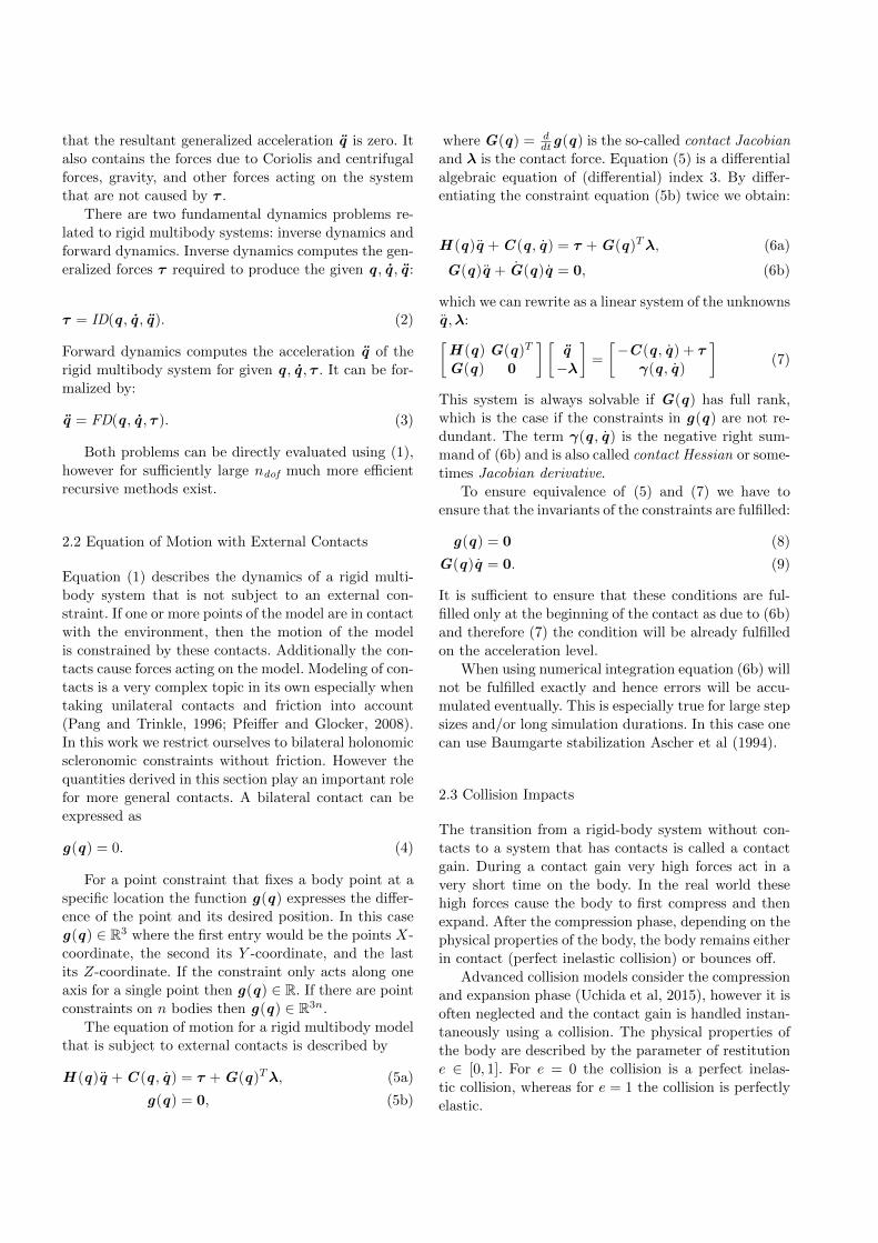
Martin L. Felis
Received: 20 October 2014 / Accepted: 13 May 2016
This is a preprint of Martin L. Felis, RBDL - an Efficient Rigid-Body Dynamics Library using Recursive Algorithms,Autonomous Robots, 2016, DOI 10.1007/s10514-016-9574-0.The final version is available from: http://link.springer.com/article/10.1007/s10514-016-9574-0.
Abstract In our research we use rigid-body dynamics
and optimal control methods to generate 3-D whole-
body walking motions. For the dynamics modeling and
computation we created RBDL - the Rigid Body Dy-
namics Library. It is a self-contained free open-source
software package that implements state of the art dy-
namics algorithms including external contacts and colli-
sion impacts. It is based on Featherstone’s spatial alge-
bra notation and is implemented in C++ using highly
efficient data structures that exploit sparsities in the
spatial operators. The library contains various helper
methods to compute quantities, such as point velocities,
accelerations, Jacobians, angular and linear momentum
and others. A concise programming interface and mini-
mal dependencies makes it suitable for integration into
existing frameworks. We demonstrate its performance
by comparing it with state of the art dynamics libraries
both based on recursive evaluations and symbolic code
generation.
Keywords reduced coordinates, rigid-body dynamics,
Jacobian, contact, software
1 Introduction
A lot of research of rigid multibody dynamics algo-
rithms has been done over the last decades. The the-
ory of multibody dynamics has been the subject of
various textbooks such as Khalil and Dombre (2004);
Craig (2005); Jain (2011), and others. Various algo-
rithms have been derived that solve fundamental dy-
Martin L. FelisResearch Group Optimization in Robotics and BiomechanicsInterdisciplinary Center for Scientific Computing (IWR),ML 100, Berliner Str. 45, 69120 Heidelberg, GermanyE-mail: [email protected]
namics related problems or compute various quantities
very efficiently. Not only the theory but also the for-
mulation and notation of dynamics has been improved.
Traditionally the equation of motion is described using
two 3-D equations, one for linear movement and one for
rotational movement. When analyzing systems of con-
nected bodies, this quickly results in a large amount of
equations (Luh et al 1980; Armstrong 1979) that are
both difficult to read and transform into programming
code. To circumvent this, alternate formulations based
on screw theory (Ball 1900) have been proposed and
proved to be very useful to analyze derive and formu-
late various algorithms (Featherstone 1983; Rodriguez
1987; Rodriguez et al 1988; Jain and Rodriguez 1993).
An overview of state of the art dynamics algorithms
and a brief historical overview on dynamics algorithms
has been composed in Featherstone and Orin (2000).
There are in general two classes of dynamics algo-
rithms: maximal coordinate algorithms on the one side
and reduced coordinates algorithms on the other side.
Maximal coordinate approaches model each body indi-
vidually and use joint constraint equations to restrict
the relative motions of the bodies. The methods allow to
handle certain closed loops systems more easily however
the constraint equations, including joint constraints,
may not be fulfilled at all times and cause separation of
connected bodies. Well known implementations of this
approach is ODE and Bullet that are commonly used
in video games as well as in robotic applications.
Reduced (or generalized) coordinate algorithms
usually assume multibody systems for which the topol-
ogy can be described by a tree. These algorithms have
the advantage to only operate on the actual degrees of
freedom of the system that fulfill the joint constraints
at all times. They operate on much smaller systems
than the maximal coordinate approaches however the
algorithms are usually more complex and difficult to
implement. A well known algorithm that usually is
described using reduced coordinates is the Recursive
Newton-Euler Algorithm. Simulation of systems sub-
ject to external contacts violate the tree topology as-
sumption and require special treatment that further in-
crease complexity when implementing these.
Dynamics algorithms can be implemented in two
ways: by implementing the algorithms directly as com-
puter code or by implementing them in a computer al-
gebra software to formulate symbolic expressions of the
result of these algorithms and convert the expressions
to computer code. We refer to the former approach as
recursive methods and the latter as symbolic code gen-
eration.
Symbolic code generation tools can easily prune out
expressions that are zero. For planar models this will
automatically remove all computations that are not
within the plane the model is defined. Disadvantages
of these approaches are that the symbolic expressions
are reduced to scalar expressions which may not be ex-
ploited by modern CPUs. Further, the generation itself
can be time consuming and the output is very complex
and can only be used as black box. Whenever a change
of the model is required one has to generate the code
anew.
Recursive methods have the advantage that they are
self-contained and do not need a computer algebra to
create code for a new model. New methods can easily be
implemented and used by existing models. The code can
be analyzed and shared expressions can be extracted
into separate functions such that redundant computa-
tions can be avoided. This approach leads to vector val-
ued expressions in the computer code that allows forfast evaluations using SIMD (Single Instruction, Mul-
tiple Data) instructions present in today’s CPUs.
The aim of this paper is twofold: first we give an
overview of available state of the art algorithms for
reduced coordinate rigid-body dynamics with external
contacts together with formulations to compute quan-
tities that are often needed in simulation and control,
such as Jacobians, system angular momentum, and oth-
ers. Second we present RBDL – the Rigid Body Dy-
namics Library, which is a mature, thoroughly tested,
and highly efficient publicly available open-source im-
plementation of all the presented algorithms and formu-
lations based implemented as recursive methods. We
demonstrate its performance by various benchmarks,
including comparison to a state of the art dynamics li-
brary and code generation tool for models of different
sizes.
The structure of the paper is the following: Section 2
describes the basic formulation of rigid-body dynamics
of arbitrarily branched trees, also with external con-
tacts. Section 3 gives a brief introduction to spatial al-
gebra and Section 4 describes how we model multibody
systems. The following Section 5 presents the state of
the art algorithms: the Recursive Newton-Euler Algo-
rithm (RNEA) for inverse dynamics, the Composite
Rigid-Body Algorithm (CRBA) to compute the joint
space inertia matrix, and the Articulated Body Algo-
rithm (ABA) to compute the forward dynamics. In Sec-
tion 6 we show how various quantities such as 3-D point
velocities and accelerations, Jacobians, system angular
momentum and others can be computed. In Section 7
we discuss implementation details of our open-source
dynamics library RBDL and in Section 8 we evalu-
ate the performance of our implementation with that
of other implementations both using recursive methods
and symbolic code generation.
2 Theoretical Background
The theory of rigid-body dynamics is the focus of many
textbooks (for a small selection refer to the introduc-
tion). In the following we borrow large parts of the de-
scription and notation used in Featherstone (2008).
2.1 Equation of Motion for Rigid Multibody Systems
For a given rigid multibody model with ndof ∈ Rndegrees of freedom we use generalized coordinates to
describe the state of the system. We use the symbols
q(t), q(t), q(t), τ (t) ∈ Rndof to denote the generalized
positions, generalized velocities, generalized accelera-
tions, and generalized forces of the system at the cur-rent time t ∈ R. Throughout this paper we consider the
dynamics at the current instant and we therefore omit
the argument t of the generalized variables.
The dynamics of rigid multibody systems using gen-
eralized coordinates is described by the equation:
H (q)q + C (q , q) = τ (1)
The matrix H (q) ∈ Rndof×ndof is the symmetric and
positive definite joint space inertia matrix or general-
ized inertia matrix. The term C (q , q) ∈ Rndof is the
Coriolis term or generalized bias force and τ the gen-
eralized force applied at the joints. For underactuated
systems with nactuated < ndof actuated degrees of free-
dom these generalized forces can be written as τ = Tu ,
where u ∈ Rnactuated are the forces of the actuated joints
and the matrix T ∈ Rndof×nactuated maps those onto the
generalized forces.
The generalized bias force (also sometimes called
”nonlinear effects”) is equal to the amount of general-
ized force that has to be applied to the system such
that the resultant generalized acceleration q is zero. It
also contains the forces due to Coriolis and centrifugal
forces, gravity, and other forces acting on the system
that are not caused by τ .
There are two fundamental dynamics problems re-
lated to rigid multibody systems: inverse dynamics and
forward dynamics. Inverse dynamics computes the gen-
eralized forces τ required to produce the given q , q , q :
τ = ID(q , q , q). (2)
Forward dynamics computes the acceleration q of the
rigid multibody system for given q , q , τ . It can be for-
malized by:
q = FD(q , q , τ ). (3)
Both problems can be directly evaluated using (1),
however for sufficiently large ndof much more efficient
recursive methods exist.
2.2 Equation of Motion with External Contacts
Equation (1) describes the dynamics of a rigid multi-
body system that is not subject to an external con-
straint. If one or more points of the model are in contact
with the environment, then the motion of the model
is constrained by these contacts. Additionally the con-
tacts cause forces acting on the model. Modeling of con-
tacts is a very complex topic in its own especially when
taking unilateral contacts and friction into account
(Pang and Trinkle, 1996; Pfeiffer and Glocker, 2008).
In this work we restrict ourselves to bilateral holonomic
scleronomic constraints without friction. However the
quantities derived in this section play an important role
for more general contacts. A bilateral contact can be
expressed as
g(q) = 0. (4)
For a point constraint that fixes a body point at a
specific location the function g(q) expresses the differ-
ence of the point and its desired position. In this case
g(q) ∈ R3 where the first entry would be the points X-
coordinate, the second its Y -coordinate, and the last
its Z-coordinate. If the constraint only acts along one
axis for a single point then g(q) ∈ R. If there are point
constraints on n bodies then g(q) ∈ R3n.
The equation of motion for a rigid multibody model
that is subject to external contacts is described by
H (q)q + C (q , q) = τ + G(q)Tλ, (5a)
g(q) = 0, (5b)
where G(q) = ddtg(q) is the so-called contact Jacobian
and λ is the contact force. Equation (5) is a differential
algebraic equation of (differential) index 3. By differ-
entiating the constraint equation (5b) twice we obtain:
H (q)q + C (q , q) = τ + G(q)Tλ, (6a)
G(q)q + G(q)q = 0, (6b)
which we can rewrite as a linear system of the unknowns
q ,λ:[H (q) G(q)T
G(q) 0
] [q−λ
]=
[−C (q , q) + τ
γ(q , q)
](7)
This system is always solvable if G(q) has full rank,
which is the case if the constraints in g(q) are not re-
dundant. The term γ(q , q) is the negative right sum-
mand of (6b) and is also called contact Hessian or some-
times Jacobian derivative.
To ensure equivalence of (5) and (7) we have to
ensure that the invariants of the constraints are fulfilled:
g(q) = 0 (8)
G(q)q = 0. (9)
It is sufficient to ensure that these conditions are ful-
filled only at the beginning of the contact as due to (6b)
and therefore (7) the condition will be already fulfilled
on the acceleration level.
When using numerical integration equation (6b) will
not be fulfilled exactly and hence errors will be accu-
mulated eventually. This is especially true for large step
sizes and/or long simulation durations. In this case one
can use Baumgarte stabilization Ascher et al (1994).
2.3 Collision Impacts
The transition from a rigid-body system without con-
tacts to a system that has contacts is called a contact
gain. During a contact gain very high forces act in a
very short time on the body. In the real world these
high forces cause the body to first compress and then
expand. After the compression phase, depending on the
physical properties of the body, the body remains either
in contact (perfect inelastic collision) or bounces off.
Advanced collision models consider the compression
and expansion phase (Uchida et al, 2015), however it is
often neglected and the contact gain is handled instan-
taneously using a collision. The physical properties of
the body are described by the parameter of restitution
e ∈ [0, 1]. For e = 0 the collision is a perfect inelas-
tic collision, whereas for e = 1 the collision is perfectly
elastic.

The contact gain is a discontinuous change in the
generalized velocity variables from q− to q+, i.e. the
velocity before the collision to the velocity after the
collision. The change can be computed using:[H (q) G(q)T
G(q) 0
] [q+
−Λ
]=
[H (q)q−
−eG(q)q−
](10)
where Λ is the contact impulse. The upper part of this
equation implies:
H (q)q+ −H (q)q− = G(q)TΛ (11)
which is the change of momentum of the system due to
the collision. The lower part
G(q)q+ = −eG(q)q− (12)
states what the contact velocity is after the collision.
For e = 0 this is equivalent to a contact velocity of
zero, a perfect inelastic collision.
In the following we may omit the arguments q , q for
the quantities when their requirement should be clear
from the context.
3 Spatial Algebra
Traditionally the dynamics of rigid bodies are described
by two sets of 3-D equations: one 3-D equation for
the linear (translational) motions and forces and one
3-D equation for the rotational (angular) motions and
forces. Spatial algebra is a notation for rigid body mo-
tions and dynamics that embeds the two types of 3-D
equations in a single 6-D equations. A more complete
introduction can be found in Featherstone (2010).
3.1 Elements of Spatial Algebra
The fundamental elements of spatial algebra are spa-
tial motions v ∈ M6, spatial forces f ∈ F6 and spatial
inertias I : M6 → F6. By using Plucker bases DO, EOFeatherstone (2006) we have a mapping DO : R6 → M6
and EO : R6 → F6.
3.1.1 Motion and Force Vectors
A spatial velocity vector describes both linear and an-
gular velocity of a rigid body and is of the form:
v =
[ω
vO
]= [ωx, ωy, ωz, vOx, vOy, vOz, ]
T(13)
where O is an arbitrary but fixed reference point. The
3-D vector ω ∈ R3 describes the angular velocity of the
body about an axis that passes through O and vO ∈ R3
is the linear velocity of the body point that currently
coincides with the reference point O.
A spatial force vector describes both linear and ro-
tational force components that act on a body and is of
the form:
f =
[nO
f
]= [nOx, nOy, nOz, fx, fy, fz, ]
T(14)
where nO ∈ R3 describes the total moment about the
point that coincides with O and f ∈ R3 the linear force
along an axis passing through O.
3.1.2 Spatial Inertia
The spatial inertia can be expressed as a 6× 6 matrix:
I =
[IC +mc × c×T mc×
mc×T m1
](15)
where IC is the inertia of the body at the center of
mass, c is the 3-D coordinate vector of the center of
mass, and m is the mass of the body.
For a body with spatial velocity v and spatial inertia
I we can compute the spatial momentum as h = I v .
One should note that h ∈ F6.
3.1.3 Spatial Transformations
In practice it is useful to use different coordinate frames,
such as body local coordinate frames, instead of per-
forming computations in one single coordinate frame.
Spatial algebra provides a convenient way to transform
spatial quantities such as motions, forces, and inertias
between coordinate frames.
If A and B are two coordinate frames where B is
translated by r ∈ R3 and also rotated as described by
the orthonormal matrix E ∈ R3×3 we can then define
the following spatial transformations:
BXA =
[E 0
−Er× E
], BX∗A =
[E −Er×0 E
](16)
with r× being the skew symmetric matrix of the vector:
xyz
× =
0 −z y
z 0 −x−y x 0
. (17)
Elements of M6 are transformed using BXA whereas
elements of F6 are transformed using BX∗A. Similarly
the inverse transformations AXB and AX∗B can be de-
fined. For given E and r we may also write the spatial
transformation as X(E , r).
The motion vector Am ∈ M6 and the force vectorAf ∈ F6 that are described in coordinate frame A can
be transformed to the coordinate frame B using
Bm = BXAAm (18)
B f = BX∗AAf . (19)
As spatial inertias are mappings from M6 to F6 the
transformation of spatial inertia AI that is described in
frame A can be transformed to frame B by:
B I = BX∗AAIAXB . (20)
3.1.4 Spatial Cross Products
When looking at rigid motions using 3-D equations the
cross product has a special property: if we have a vectorAu ∈ R3 that is fixed in a frame A moves with an
angular velocity of AωA then the derivative of Au is:
u = AωA × Au(t). (21)
In spatial algebra there are two cross product oper-
ators: one for motion vectors:
mO× =
[ω
vO
]× =
[ω× 0
v× ω×
], (22)
and one for force vectors:
v×∗ =
[ω
vO
]×∗ =
[ω× vO×0 ω×
], (23)
3.1.5 Spatial Equation of Motion
The equation of motion for a single rigid-body ex-
pressed using Spatial Algebra is stated by:
f = I a + v ×∗ I v (24)
= I a + p. (25)
Here f = [nO, f ]T
is the spatial force acting on a
body where nO is the total moment applied at point O
and f the linear force that is acting on a line passing
through O. The spatial acceleration a = [ω, vO]T
con-
sists of ω which is the rotational acceleration around
an axis passing through O and the linear acceleration
vO. The quantity p is sometimes called the spatial bias
force, which equals to the spatial force that has to be
applied to the body, such that no acceleration is pro-
duced on the body.
3.1.6 Comparison with the Traditional 3-D Notation
The spatial algebra equation of motion of a single rigid-
body embeds the traditional 3-D equations of motion
by:[nC
f
]=
[IC 0
0 m1
] [ω
c − ω × vC
]+
[ω× vC×0 ω×
] [IC 0
0 m1
] [ω
vC
](26)
=
[ICω + ω × ICω
mc
]. (27)
Here the reference point C is assumed to be coincident
with the center of mass of the body and c is the linear
acceleration of the center of mass.
It is important to emphasize that spatial algebra is
not simply a matter of notation that concatenates the
two 3-D equations. Instead, it performs operations on a
different level of abstraction. Traditional 3-D equations
express the motion of rigid bodies using quantities ex-
pressed at points that are moving with the body, e.g.
the linear velocity of the center of mass and the angu-
lar velocity. In spatial algebra however the quantities
are expressed at arbitrary but fixed reference points in
space. Spatial velocities describe the flow of the body
at the reference point, i.e. the angular and linear veloc-
ity of the point body that currently coincides with the
point. Spatial accelerations describe the rate of change
of this flow, i.e. how the angular and linear velocity of
the point that coincide with the reference point change
over time.
The difference of spatial velocity and acceleration
compared to the classical formulation can seen by con-
sidering a body with constant angular velocity ω. In
the classical 3-D formulation one would describe the
motion of a body in terms of linear and angular ve-
locity (rP and ω) and linear and angular acceleration
(rP and ω) of a point P that moves with the body. If
that point P does not lie on the axis of rotation then
the linear acceleration rP 6= 0 and points towards the
axis of rotation. In spatial algebra however, the spa-
tial acceleration a i of body i is the time derivative of
the spatial velocity v i. A constant v i therefore results
in a i = 0. For a thorough comparison of classical and
spatial accelerations we refer to Featherstone (2001).
4 Modeling of Rigid Multibody Systems
In this section we present the rigid multibody model for-
mulation that is used in the description of algorithms
below and as the main data structure of the software

RBDL. It follows the notation and formulation pre-
sented in Featherstone (2008).
A rigid multibody system (MBS) consists of a set of
bodies that are interconnected by joints. A joint always
connects two bodies and in general affects the relative
motion of the bodies.
The variables that describe a rigid multibody model
with nB ∈ N bodies are listed in Table 1
λi Index of the parent body index for joint i thatconnects body i with body λi.
κ(i) The set of joints that influence (i.e. support)body i.
µ(i) The set of children of joint i.ν(i) The subtree that starts at joint i.S i Motion space matrix for joint ivi Spatial velocity of body ici Velocity dependent acceleration term of body iai Spatial acceleration of body if i Spatial force body i is acting on the parent body
λi via the connecting jointiX0 Spatial transformation from the global frame to
the frame of body iiXλi Spatial transformation from the parent of body
i to body iXTi Spatial transformation from the parent of body
i to the frame of joint iI Spatial inertia of body iI c Composite body inertia of body iIA Articulated body inertia of body ipA Articulated bias force of body i
Table 1 Variables of a loop-free rigid multibody model
4.1 Coordinate Frames and Transformations
There are multiple coordinate frames involved when de-
scribing a multibody system. First there is the global
reference frame which we name 0. This system is fixed
and does not move. The root body B0 is attached to
this global reference frame and also defines a reference
frame that is defined for the body B0. We call this frame
the body (local) reference frame. In the case of B0 the
global reference frame and the body reference frame of
B0 are the same.
When we have a system with a single moving body
then this body B1 is attached via joint J1 to the base
body B0. Usually joints are not located at the origin
of the parent body. Instead they are translated and/or
rotated relative to the coordinate frame of the parent
body. This gives rise to the joint location frame. The
transformation from the parent body frame to the joint
location frame is denoted as XTi. It is fixed and spec-
ified in the parent’s body reference frame.
When a joint is moving an additional frame is re-
quired. I.e. a revolute joint changes the orientation
whereas a prismatic joint results in a translation of the
coordinate frame. The joint motion frame is the frame
that changes when the joint moves and is denoted as
XJi.
The transformation from the parent body to the
child body is then given by
iXλi = XJiXTi.
4.2 Bodies
A single body in a rigid multibody system is described
by its mass m, the location of the center of mass c ∈ R3
and its inertia tensor IC ∈ R3×3 at the center of mass.
These values are taken to construct the spatial inertia
matrix I i ∈ R6×6 for each body i.
4.3 Joints
A joint always connects two bodies with each other and
in general limits the relative motion between them. A
joint may allow between 0 and 6 degrees of freedom,
for which 0 degrees of freedom mean that it is a fixed
joint (i.e. the two bodies are rigidly connected with each
other) and a joint with 6 degrees of freedom (also called
free-flyer joint) does not impose any restriction on the
relative motion.
For each joint a specific subset of the generalized
state variables are associated with the joint. For joint i
with ns degrees of freedom the value q i ∈ Rns are the
associated generalized joint positions of joint Ji and
similarly q i, q i, τ i ∈ Rns are the associated generalized
joint velocities, accelerations and forces for that joint.
τ i are more specifically the forces that are transmitted
via the joint i. The tuple (q i, q i, q i, τ i) is referred to
as the joint state.
If the generalized joint positions for joint i are
nonzero, then the transformation caused by the joint is
represented by joint motion frame transformation XJi.
It is a spatial transformation of the form (16) where the
entries E and r depend on the type of joint.
4.3.1 Joint Models
The motion space of a joint is described by the so-
called motion subspace matrix S which defines a map-
ping S : Rns → M6. The subspace matrices for all
joints with only one degree of freedom that are either
revolute (SR·) or prismatic (ST ·) around or along the
coordinate axes are:

SRx =
1
0
0
0
0
0
, SRy =
0
1
0
0
0
0
, SRz =
0
0
1
0
0
0
,
STx =
0
0
0
1
0
0
, STy =
0
0
0
0
1
0
, STz =
0
0
0
0
0
1
.
It is also possible to define motion subspace matrices for
helical motions. In that case there are nonzero entries
in both the upper three and the lower three entries.
Once the motion subspace matrix is defined the joint
velocities and accelerations can be expressed as:
vJi = S iq i (28)
aJi = cJi + S iq i (29)
with
cJi = S iq i =
(dS i
dt+ v i × S i
)q i (30)
The value of S i is affected by two factors: first, the
change of the motion subspace matrix over time itself
and second, a change of the motion subspace matrix
due to the motion of the frame of body i. For the simple
single degree of freedom joints above, however this value
is always zero. The term cJi is also called the velocity
dependent spatial acceleration term.
4.3.2 Joints with Multiple Degrees of Freedom
Models that contain joints with multiple degrees of free-
dom (DOF) can be treated in two different ways: em-
ulate multiple degrees of freedom using multiple single
degree of freedom joints and bodies with zero inertia
and mass or the use of proper multiple degrees of free-
dom joints. The former have the advantage that they
are very simple to implement however this is at the
cost of performance as the algorithms will need more
iterations to perform the same computations.
Multiple degrees of freedom joints occur in robotics
mainly in the first movable body of the system from
which the remaining multibody system is spanned. In
humanoid robotics this body is often referred to as the
Floating Base and the joint as Floating Base Joint, or
Freeflyer Joint. In 3-D it has six degrees of freedom and
is not actuated, i.e. the generalized forces corresponding
to it are always zero.
In models for human characters such as in anima-
tions also other joints such as those of hip, ankle, and
shoulder can be modeled using 3 DOF joints. This
makes joints with 3 DOF of particular interest. Fur-
thermore when using 3 DOF joints the floating-base
can be emulated using two joints instead of six.
For joints with multiple degrees of freedom we
need to derive the expressions for E(q i), r(q i) to de-
scribe the joint motion transformation and S(q i), and
cJi(q i, q i) to express the motion subspace of the joint,
and the velocity dependent spatial acceleration term of
the joint.
A 3 DOF joint that describes the translation along
the X–, Y –, and Z– axis is described by:
E(q i) = 1 ∈ R3×3, (31)
r(q i) = (q i,0, q i,1, q i,2)T , (32)
S(q i) =
0 0 0
0 0 0
0 0 0
1 0 0
0 1 0
0 0 1
, (33)
cJi(q i, q i) = 0 ∈ M6. (34)
Rotational joints are slightly more involved due to the
amount of sinus and cosine expressions. For a spherical
joint that uses the Euler-Cardan angle convention XYZ
we use the following notation sj = sin(q i,j) and cj =
cos(q i,j) and furthermore q j = q i,j . This allows us to
write the joint model dependent expressions as:
E(q i) =
c2c1 s2c0 + c2s1s0 s2s0 − c2s1c0−s2c1 c2c0 − s2s1s0 c2s0 + s2s1c0s1 −c1s0 c1c0
,(35)
r(q i) = 0 ∈ R3, (36)
S(q i) =
c2c1 s2 0
−s2c1 c2 0
s1 0 1
0 0 0
0 0 0
0 0 0
, (37)
cJi(q i, q i) =
−s2c1q2q0 − c2s1q1q0 + c2 ∗ q2 ∗ q1
−c2c1q2q0 + s2s1q1q0 − s2q2q1
c1q1q0
0
0
0
.(38)

Joints for other conventions or more degrees of free-
dom can similarly be derived. To note here is that the
presented EulerXYZ joint suffers from singularities. An
alternative is a joint that e.g. uses Quaternions Shoe-
make (1985), which is described in Featherstone (2008).
A difficulty here is that the generalized velocities are no
more the derivatives of the generalized positions.
As suggested in Featherstone (2008) it is very conve-
nient to encapsulate the computations of the joint type
and q , q dependent computations in a so-called joint
model calculation routine:
[XJi,S i, cJi] = jcalc(jtype(i), q i, q i). (39)
The method jtype(i) returns a type of joint that will
then be used e.g. in a if . . . elseif block to chose the
actual code depending of the type.
4.3.3 Joint Numbering
The connection of bodies via joints in a loop-free system
can also be seen as a directed graph, where the joints
are the directed edges and the bodies are the nodes.
Apart from the root body there are the same number
of bodies Bi as joints Ji with i = 1, . . . , nB .
Every joint connects always exactly two bodies.
Joint i connects bodies Bλi with body i. The body with
index λi is also called the parent body and λ is called
the parent array. The bodies and joints are numbered
such that
λi < i (40)
always holds. If κ(i) is the set of joint indices that in-
fluence body i then this numbering has the property
j < i, ∀j ∈ κ(i).
This numbering becomes especially useful when
computations require that all parent joints (i.e. all
joints in κ(i)) must have been performed before a com-
putation for body Bi can be done, as it is sufficient
having computed the values for all bodies with j < λi.
Another important set of indices is µ(i) which con-
tains the indices of all joints that are contained in the
subtree starting at index i.
5 Dynamics Algorithms
In this section we present algorithms that allow us to
compute the quantities required for the evaluation of
the equation of motion presented in Section 2.1. Some
of the algorithms are the most efficient algorithms avail-
able for their tasks and all algorithms and methods are
implemented in the software package RBDL.
5.1 Recursive Newton-Euler Algorithm
The Recursive Newton-Euler Algorithm (RNEA) is a
highly efficient algorithm for the computation of inverse
dynamics of a branched rigid-body model. It has an al-
gorithmic complexity of O(nB) where nB is the number
of movable bodies in the multibody system.
It performs the computation in three steps:
1. Compute the position, velocity, and acceleration of
all bodies.
2. Use (25) to compute for each body the net force that
causes the previously computed acceleration.
3. Compute the force that is transmitted over each
joint.
Pseudo code for the whole algorithm is presented
in Algorithm 1. The acceleration of the root body is
initialized with ag = [0, g ]T ∈ M6, where g ∈ R3 is
the gravity vector in global coordinates. As the accel-
erations are propagated from joint to joint this ensures
that gravity is applied to every body.
1 v0 = 02 a0 = −ag3 for i = 1, . . . , nB do4 [XJi,S i, cJi] = jcalc(jtype(i), qi, qi)5
iXλi = XJiXTi
6 if λi 6= 0 then7
iX0 = iXλiλiX0
8 end9 vJi = S iqi
10 aJi = cJi + S iqi11 vi = iXλivλi + vJi
12 ai = iXλiaλi + aJi
13 f i = I iai + vi ×∗ I ivi − iX∗0 f xi14 end15 for i = nB , . . . , 1 do16 τ i = STi f i17 if λi 6= 0 then18 f λi = f λi + λiX∗i f i19 end
20 end
Algorithm 1: Recursive Newton-Euler Algorithm
The presented algorithm can be applied on kine-
matic trees and for all scleronomic joints including revo-
lute, prismatic, and helical joints. Furthermore it allows
to compute the inverse dynamics in presence of exter-
nal forces f xi ∈ F6. The algorithm can also be used to
compute the generalized bias term in (1) C (q , q) by
setting q = 0.
5.2 Composite Rigid-Body Algorithm
The Composite Rigid-Body Algorithm (CRBA) com-
putes the joint space inertia matrix H (q). The algo-

rithm proceeds recursively and only computes the en-
tries of the matrix that are nonzero. The algorithm can
be motivated by looking at the computation for the
multibody system’s kinetic energy which can be stated
as:
T =1
2qTH q =
1
2
ndof∑i=1
ndof∑j=1
Hij qiqj (41)
Alternatively, the kinetic energy of the system can be
seen as the sum of the kinetic energy of the individual
bodies:
T =1
2
nB∑i=1
vTi I iv i. (42)
Without loss of generality we can assume that all mo-
tion subspace matrices are expressed in the global ref-
erence frame. This allows us to write (42) as:
T =1
2
nB∑k=1
∑i∈κ(k)
∑j∈κ(k)
qTi STi I kS j q j . (43)
This equation expresses the kinetic energy as a sum over
all combinations where body k is supported by both the
joint i and j. This can be reformulated to
T =1
2
nB∑i=1
nB∑j=1
∑k∈ν(i)∩ν(j)
qTi STi I kS j q j (44)
=1
2
nB∑i=1
nB∑j=1
qTi H ij q j (45)
with
H ij =∑
k∈ν(i)∩ν(j)
STi I kS j . (46)
Equation (43) can be seen as assembling all the re-
quired quantities from k up to the root of the graph,
whereas equation (44) performs the same computation
by assembling the quantities down the subtrees starting
at the joint that is influenced by both i and j.
The expressions H ij and H ji correspond to the
block of the joint space inertia matrix that are affected
by the joint variables of joints i and j. Due to the cho-
sen joint numbering we can simplify the union of the
two sets using:
ν(i) ∩ ν(j) =
ν(i) if i ∈ ν(j)
ν(j) if j ∈ ν(i)
∅ otherwise
(47)
Together with
I ci =∑j∈ν(i)
I j (48)
we can further simplify H ij as:
H ij =
STi I ciS j if i ∈ ν(j)
STi I cjS j if j ∈ ν(i)
0 otherwise.
(49)
The Composite Rigid-Body Algorithm is presented
as pseudo code in Algorithm 2.
1 H = 02 for i = 1, . . . , nB do3 I ci = I i4 end5 for i = nB , . . . , 1 do6 if λi 6= 0 then7 I cλi = I cλi + λiX∗i I ci
iXλi8 end9 F = I ciS i
10 H ii = STi F11 j = i12 while λi 6= 0 do13 F = λiX∗j F
14 j = λi15 H ij = FTSj16 H ji = HT
ij
17 end
18 end
Algorithm 2: Composite Rigid-Body Algorithm
The presented algorithm assumes that the spatial
transformations from parent to child iXλi and the joint
motion subspace matrices S i have already been com-
puted. If this is not the case then this could be done
in the first loop. Furthermore, the quantities S i and I ciare expressed in body local coordinates.
5.3 Articulated Body Algorithm
The Articulated Body Algorithm (ABA) allows to com-
pute the forward dynamics of a kinematic tree with
O(nB) operations. It was first described by Feather-
stone in Featherstone (1983) however different variants
have been described by others as shown in Jain (1991).
We only outline the algorithm here. For a complete
derivation including some variation in the formulation
we refer to Featherstone (2008).
One of its key concepts is the articulated-body iner-
tia which captures the dynamic properties of a body
that is connected to other bodies and how it reacts
when a force is applied to it while taking the connect-
ing bodies into account. The equation of motion for an
articulated body is given by:
f = IAa + pA (50)

where IA is the articulated body inertia and pA is the
articulated bias force.
The articulated body inertia and articulated bias
force can be recursively computed. For body i the com-
putations are:
IAi = I i +∑j∈µ(i)
I aj (51)
pAi = pi +∑j∈µ(i)
paj (52)
with
I aj = IAj − IAj S j(S jIAj S j)
−1STj IAj (53)
paj = pAj + I ajcj + IAj S j(STj IAj S j)
−1(τ j − STj pAj ).
(54)
The algorithm proceeds in three steps:
1. Compute positions, velocities and rigid-body bias
forces from base outwards.
2. Compute the articulated body inertias and articu-
lated bias forces.
3. From base outwards: use IAi and pAi computed in
the previous step to compute the joint accelerations
using:
q i = (STi IAi ST
i )−1(τ i − STi (IAi aλi + ci)− ST
i pAi )
(55)
Pseudocode for the algorithm is shown in Algorithm
3. The code presented here avoids redundant computa-
tions of shared terms in Equations (53) and (54).
The Articulated Body Algorithm can be modified
to yield a O(nB) solution operator to solve the linearsystem H (q)q = τ for the accelerations q . To do so the
acceleration due to gravity and all velocity dependent
variables in the first loop must be set to zero. Only the
articulated bias forces pA are influenced by τ . When
solving the system for multiple values of q one should
therefore avoid the costly re-evaluation of the articu-
lated body inertias IA and only compute them once.
6 Kinematics, Energy, and Momentum
Computations
In simulations and analysis of rigid multibody systems,
it is often required to compute 3-D coordinates, 3-D
linear velocities, and 3-D linear accelerations of points
that are fixed on a body. This requires some clarifi-
cations, as spatial motion vectors describe the flow of
motion at a specified point.
In this section the point P that is rigidly attached
to and therefore moving with the body i in body local
1 v0 = 02 a0 = −ag3 for i = 1, . . . , nB do4 [XJ ,S i, cJi] = jcalc(jtype(i), qi, qi)5
iXλi = XJXTi
6 if λi 6= 0 then7
iX0 = iXλiλiX0
8 end9 vJi = S iqi
10 vi = iXλivλi + vJi
11 ci = cJi + vi × vJi
12 IAi = I i13 pAi = vi ×∗ I ivi − iX∗0 f xi14 end15 for i = nB , . . . , 1 do16 U i = IAi S i17 Di = STi U i
18 ui = τ i − STi pAi19 if λi 6= 0 then
20 Ia = IAi −U iD−1i UT
i
21 pa = pAi + Iaci + U iD−1i ui
22 IAλi = IAλi + λiX∗i Ia iXλi23 pAλi = pAλi + λiX∗i pa24 end
25 end26 for i = 1, . . . , nB do27 a ′ = iXλiaλi + ci
28 qi = D−1i (ui −UT
i a ′)29 ai = a ′ + S iqi30 end
Algorithm 3: Articulated Body Algorithm
coordinates irP ∈ R3. In this section we are interested
in computing the classical 3-D expressions of linear ve-
locity, linear acceleration of the point P . Furthermore
we want to formulate the contact Jacobian and contact
Hessian for this point.
6.1 Point Velocities
The velocity of the fixed body point can be computed
using:
P ′ v i =
[P ′ωP ′vP ′
]i
= X(0ETi ,
irP )iv i (56)
where 0E i is the orientation of body i with respect to
the orientation of the global frame. The spatial motion
vector v i is transformed to a coordinate frame P ′ for
which the reference point coincides with the global co-
ordinates of P and also has the same orientation as
the global reference frame. The lower part of P′vP is
therefore expressed at the point of body i that currently
coincides with P and therefore we have P ′vP ′ = 0rP .
In RBDL the function CalcPointVelocity
(model, q, qdot, body id, point position) per-
forms this computition and returns the 3-D vectorP ′vP ′ .

6.2 Point Accelerations
To compute the acceleration rP of the body fixed point
P we can use:
P ′ a ′i =
[P ′ωP ′aP ′
]i
= X(0ETi ,
irP )ia i+
[0
P ′ω × P ′vP ′
].
(57)
The first term on the right-hand side transforms the
spatial acceleration from body i coordinates to the co-
ordinate frame of P ′ (i.e. the same coordinate frame as
above). The second term compensates for the fact that
spatial acceleration is not the acceleration of the ref-
erence point of the coordinate frame but instead it is
the rate of change of flow at the reference point of the
coordinate system.
In RBDL the function CalcPointAcceleration
(model, q, qdot, qddot, body id,
point position) performs this computition and
returns the 3-D vector P′aP ′ .
6.3 Contact Jacobians
For a given joint configuration q , the contact Jacobian
from (5) maps from the generalized velocities q to the
spatial velocity of a body expressed in some coordinate
frame A:
Av j = AG(q)q =
[AGω(q)AGvA(q)
]q (58)
AG(q) is a 6×ndof matrix, where the upper three rowsAGω(q) map onto the angular velocity of the body and
the bottom three rows AGvA(q) map onto the linear ve-
locity of Av j . All columns with index i /∈ κ(j) are zero.
The values of the non-zero columns can be obtained by
rewriting (58) as:
AG(q)q =∑i∈κ(j)
AXiv i =∑i∈κ(j)
AXiS iqi. (59)
The nonzero columns of the Jacobian can therefore be
obtained by transforming the joint motion space matri-
ces to the coordinate frame A. By using the coordinate
frame P ′ from the previous paragraphs one can com-
pute the Jacobian for the body fixed point P .
6.4 Contact Hessians
When differentiating the algebraic constraint equation
twice we obtain:
d2
dt2g(q) = G(q)q + G(q)q (60)
= G(q)q − γ(q , q) (61)
where γ(q , q) is also called the contact Hessian. In
RBDL it is computed using the same equations as the
point acceleration equations (57) and setting q = 0.
6.5 System Mass, Center of Mass, Linear, Angular,
and Centroidal Momentum
Using spatial algebra we can also compute the system’s
spatial inertia which is the inertia the system would
have if we lumped all bodies to a single body. It is
obtained using:
0I =
nB∑i=1
0X∗i I iiX0 (62)
The diagonal elements in lower right 3 × 3 submatrix
of 0I will all contain the value of the system’s total
mass. The lower left 3×3 matrix contains the expression
mc×T , where c is the location of the system’s Center
of Mass (CoM) for which the 3-D vector can easily be
extracted.
For a single rigid body its spatial momentum is
h = I v which is an element of F6. Together with the
spatial transformations we can write the system’s spa-
tial momentum expressed at the origin of the global
reference frame as:
0h =
nB∑i=1
0X∗i I iv i. (63)
The linear part of this vector will contain the linear
momentum of the system which allows us to obtain the
linear velocity of the CoM by dividing it by the sys-
tem’s total mass. The upper part contains the system’sangular momentum expressed at the origin of the global
coordinate system. Using the CoM’s location we can get
the Centroidal momentum Orin and Goswami (2008) as
the upper 3-D vector of:
CoMX00h . (64)
7 Implementation Notes
RBDL is implemented in a small subset of C++ and
the programming interface could be relatively easily ex-
posed to pure ANSI C. The library is self-contained and
does not require any additional packages. For optimal
performance it is however advised to use the C++ lin-
ear algebra package Eigen3 (Guennebaud et al, 2010).
The programming interface itself has a model-based fo-
cused structure meaning that most calls take the model
as their first argument. This also emphasizes the inde-
pendence of model and the algorithms. The library also
allows loading of models described in the URDF format.

The library is also extensively tested. At the time of
writing there are more than 200 automated tests that
ensure correctness of the library. Each test ensures the
correctness of specific properties of our implementation,
e.g. that the structure exploiting spatial algebra oper-
ators give the same results as the full 6-D formulation,
the inverse dynamics computation is consistent with the
forward dynamics computation. There is a wide range
of different models that are used in the tests: from sim-
ple pendulums to a humanoid model with 36 degrees
of freedom. Having a wide range of tests and testing
infrastructure has helped us considerably to fix errors
and gives us great confidence in the correctness of the
library, also when major code changes have to be done.
The tests run in less than a second which allows us to
run the tests very frequently during development and
to detect errors early on.
An example for the RBDL programming interface
is shown in Algorithm 4. It creates a 3-D triple pen-
dulum and computes the forward dynamics using the
Articulated Body Algorithm and prints out the gener-
alized acceleration.
7.1 Model Structure
The model structure contains all variables listed in Ta-
ble 1 and additional variables such as optional names
(i.e. strings) for each body. The individual entries of
the model structure are stored in arrays which store
the entries for each body sequentially in memory.
7.2 Constraint Sets
External contacts are modeled in RBDL using so-called
constraint sets. A constraint set contains the data nec-
essary to formulate all external contact constraints that
currently act on the body. This includes a list of bod-
ies, body points, and world normals which are used to
compute the contact Jacobians and contact Hessians.
Additionally it contains preallocated workspace for the
linear system that has to be solved during the contact
dynamics computation.
An example code is shown in Algorithm 5. Here
we add three constraints to a body. The constraints
all act on the same body point and constrain the
motion of the point in all cardinal directions. After
this we bind the constraint set to the model. This
causes the workspace to be allocated and must be per-
formed before computing the contact dynamics by call-
ing ForwardDynamicsContactsDirect (...).
1 #include "rbdl.h"
2 #include <iostream>
3
4 using namespace RigidBodyDynamics;
5 using namespace RigidBodyDynamics::Math;
6
7 int main (int argc, char* argv[]) {8 Model model;
9 Joint joint rot zyx (
10 SpatialVector (0., 0., 1., 0., 0., 0.),
11 SpatialVector (0., 1., 0., 0., 0., 0.),
12 SpatialVector (1., 0., 0., 0., 0., 0.)
13 );
14 Body body (0.1, Vector3d (0., 0., -1.),
15 Matrix3d (
16 0.1, 0., 0.,
17 0., 0.1, 0.,
18 0., 0., 0.1)
19 );
20
21 model.gravity = Vector3d (0., 0., -9.81);
22 unsigned int body 1 id = model.AddBody (
23 0,
24 Xtrans (Vector3d ( 0., 0., 0.)),
25 joint rot zyx,
26 body);
27 unsigned int body 2 id = model.AddBody (
28 body 1 id,
29 Xtrans (Vector3d ( 0., 0., -1.)),
30 joint rot zyx,
31 body);
32 unsigned int body 3 id = model.AddBody (
33 body 2 id,
34 Xtrans (Vector3d ( 0., 0., -1.)),
35 joint rot zyx,
36 body);
37
38 VectorNd q = VectorNd::Zero (model.q size);
39 VectorNd qdot =
40 VectorNd::Zero (model.qdot size);
41 VectorNd qddot =
42 VectorNd::Zero (model.qdot size);
43 VectorNd tau =
44 VectorNd::Zero (model.tau size);
45
46 ForwardDynamics (model, q, qdot, tau, qddot);
47
48 std::cout << qddot.transpose() << std::endl;
49
50 return 0;
51 }Algorithm 4: A complete RBDL example the mod-
eling and forward dynamics computation of a triple
pendulum with spherical joints that are parameter-
ized with EulerZYX angles.
7.3 Structure Exploiting Spatial Algebra
The pseudo code presented in Algorithm 1 and Algo-
rithm 2 operate on 6-D spaces, however faster formula-
tions can be derived for many spatial operations Feath-
erstone (2008).

1 ConstraintSet CS;
2
3 CS.AddConstraint (body 3 id,
4 Vector3d (0., 0., -1.),
5 Vector3d (1., 0., 0.)
6 );
7 CS.AddConstraint (body 3 id,
8 Vector3d (0., 0., -1.),
9 Vector3d (0., 1., 0.)
10 );
11 CS.AddConstraint (body 3 id,
12 Vector3d (0., 0., -1.),
13 Vector3d (0., 0., 1.)
14 );
15
16 CS.Bind(model);
17
18 ForwardDynamicsContactsDirect (model,
19 q, qdot, tau, CS, qddot);
20
21 std::cout << qddot.transpose() << std::endl;
22 std::cout << CS.force.transpose() << std::endl;
Algorithm 5: Code example for the creation of a
constraint set that adds an external point contact
to body with id body 3 id. The point is located at
(0., 0.,−1.)T in the local coordinates of the body.
An expression like Xv would cost 36 multiplica-
tions and 30 additions using 6-D arithmetic. However
the same operation can be performed by only 24 multi-
plications and 18 additions which can be seen by rewrit-
ing the multiplication using:[E 0
−Er× E
] [ω
vO
]=
[Eω
−Er × ω + EvO
](65)
=
[Eω
E(vO − r × ω)
]. (66)
The product Eω costs 9 multiplications and 6 addi-
tions, r × ω costs 6 multiplications and 3 additions,
vO−v ′ with v ′ = r ×ω costs 3 additions and the mul-
tiplication with E costs another 9 multiplications and
6 additions which totals in 24 multiplications and 18
additions.
At various points in the algorithms, it is required to
concatenate spatial transformations (16). Featherstone
introduces a compact representation plx(E , r) of the
spatial transform that only stores the orientation ma-
trix E and the linear displacement r instead of a full
6 × 6 matrix (”plx” here stands for ”Plucker transfor-
mation”). The product of two spatial transformations
X iX j =
[E i 0
−E ir i× E i
] [E j 0
−E jr j× E j
](67)
can then also be written as1:
plx(E i, r i) plx(E j , r j) = plx(E iE j , r j + ETj r i) (68)
1 The derivation exploits ETj ri × Ej = (Ej ri)×.
which only needs 33 multiplications and 24 additions
instead of 216 multiplications and 180 additions. The
plx(·, ·) data structure can also be used to efficiently
evaluate expressions Xv ,X−1v ,X∗f , and XT f .
Another expression for which drastic improvements
can be achieved is the following:
λiX∗i I ciiXλi (69)
which can be found in the Composite Rigid-Body Al-
gorithm (see Algorithm 2). It transforms the spatial in-
ertia from reference frame of body i to that of body λi.
When using 6-D operations this would result in mul-
tiplication of two 6 × 6 matrices which requires 432
multiplications and 360 additions. An alternative op-
eration can be derived that performs the same compu-
tation using 52 multiplications and 56 additions. The
faster method requires to store the spatial inertia more
compact. The 6× 6 matrix
I c =
[I mc×
mc×T m1
](70)
can be stored using 10 floating point values: 6 for the
lower triangular part of the symmetric inertia matrix I ,
3 for mc×, and an additional floating point value for m.
In Featherstone (2008) this compact structure is called
rbi(m,h , lt(I )) where lt(·) denotes the lower triangular
matrix of its argument. Using the rbi(·) structure fur-
thermore results in fewer operations when rigid body
inertias are being summed (10 additions instead of 36).
These structure exploiting operators and compact
spatial data structures yield two benefits: fewer instruc-
tions and also reduced memory consumption. The latter
also results in fewer cache misses on current CPU ar-
chitectures that further improve performance as fewer
values have to be fetched from slower memory hierar-
chies.
RBDL implements all of the mentioned compact
structures and operators. Additional structures and ex-
ploiting operators can be found in Featherstone (2008).
7.4 Reuse of Computed Values
Computing the forward dynamics using (1) requires
to compute H (q) and C (q , q). The former would be
computed using the Composite Rigid-Body Algorithm
(Algorithm 2) whereas the latter using the Recursive
Newton-Euler Algorithm (Algorithm 1) by setting q =
0. Additional computations are required when comput-
ing forward dynamics with external contacts, such as
the contact Jacobians and Hessians.
Instead of computing each from scratch one can
reuse a considerable amount of values. By first call-
ing the Recursive Newton-Euler Algorithm the values
iXλi and S i are already computed and can be reused
by the Composite Rigid-Body Algorithm. Also values
for v i are already computed that are required for the
contact Jacobians. Similarly all dependent variables for
the contact Hessians are already precomputed.
The algorithms, the model structure and the pro-
gramming interface in RBDL allow to reduce redun-
dant computations in various functions using an op-
tional boolean argument. E.g. in RBDL the function
to compute the Jacobian for a point is defined using
the following declaration:
void CalcPointJacobian (
Model &model,
const VectorNd &q,
unsigned int body_id,
const Vector3d &point_position,
MatrixNd &G,
bool update_kinematics = true
);
The last parameter update kinematics has a default
value of true. If it is not explicitly provided, it uses the
default value true. When providing false as the last
parameter RBDL reuses the existing values for AX i
and v i that are currently stored in the model structure.
8 Performance Evaluation
Performance comparisons of implementations is gener-
ally difficult as different libraries have been built with
different applications in mind. The aim of RBDL is
to efficiently evaluate the equations of motion (1) and
(7) and to compute forward and inverse dynamics of
rigid multibody systems. As performance index we use
the time duration it takes to evaluate specific quanti-
ties for a given number of times. As dynamics libraries
that are based on maximal coordinates generally do not
compute quantities explicitly we only consider the com-
parison of reduced coordinate libraries.
8.1 Floating Base Joint: Emulated vs. Multi-DOF
Many real-world systems such as humanoid robots, ve-
hicles, and biomechanical full-body human models are
underactuated. There is one designated body that has
all six degrees of freedom that is not actuated (e.g. the
Pelvis body) and all other bodies are connected to this
so-called floating-base body. The 6-D joint is referred
to as floating-base joint (or sometimes freeflyer joint).
In RBDL this floating-base joint can be modeled
either using six 1-D joints or using two 3-D joints.
To evaluate how the two modeling approaches affect
performance we created two mathematically equivalent
models of a humanoid robot with 35 degrees of free-
dom. We used the sample humanoid robot from the
OpenHRP framework (Kanehiro et al 2004). The ”em-
ulated” model which uses six 1-DOF joints for the free-
flyer joint and the ”multi-DOF” model which uses two
3-DOF joints to describe an equivalent model. For both
models we compare the performance of the O(ndof) for-
ward dynamics, the forward dynamics computation by
explicitly formulating (1) and solving it using a LLT
factorization, and the computation of all quantities of
(1) without solving it. All computations were performed
in three batches of one million evaluations and the
fastest values were used for the comparison. The results
are shown in Figure 1.
The emulated model the computations of one mil-
lion calls to the Articulated Body Algorithm took
13.83s whereas for the multi-DOF model it were 12.58s.
The alternate way to compute the forward dynamics is
to directly solve Equation (1). The fastest method we
can use here solving the system using a LLT decom-
position as the joint-space inertia matrix is symmetric
and positive definite. For the emulated model it took
21.51s to build and solve the system whereas for the
multi-DOF model it was 19.48s. We also plotted the du-
rations it takes when only building the systems: 12.24s
for the emulated model and 9.69s for the multi-DOF
model. Overall using two 3-DOF joints instead of six
1-DOF joints improves performance by about 9% when
computing forward dynamics and about 10% when eval-
uating H (q) and C (q , q).
8.2 Comparison with Existing Code
We compared the performance of RBDL with Sim-
body (Sherman et al, 2011). Simbody is a state of the
art rigid multibody simulation library that uses reduced
coordinates and recursive algorithms to compute the
multibody system dynamics using the formulations de-
scribed in Rodriguez et al (1991). The library includes a
sophisticated caching mechanism to ensure that redun-
dant computations are avoided and has a fine grained
programming interface that include special methods to
apply common operations such as H−1τ for a given τ
or G(q)Tλ without explicitly formulating the involved
matrices.
We compare the performance of RBDL and Sim-
body by comparing their implementations of a O(n)
forward dynamic operator, a linear time solution op-
erator for the expression H (q)−1τ , and repeated calls
to the former operator by calling it multiple times to
compute the inverse of the full joint space inertia ma-
trix. The last comparison measures how well both im-
EoM Setup EoM Setup +LLT Factorization
ArticulatedBody Algorithm
0
5
10
15
20
25
Dur
atio
nfo
r1.0
00.0
00ca
lls(s
)
Floating-base joint: emulated vs. multi-DOF (i7-3770)
emulatedmulti-DOF
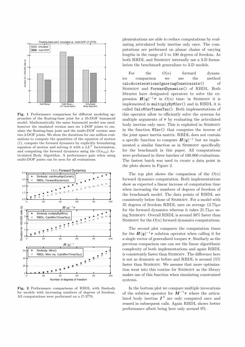
Fig. 1 Performance comparison for different modeling ap-proaches of the floating-base joint for a 35-DOF humanoidmodel. Mathematically the same humanoid model was used,however the emulated version uses six 1-DOF joints to em-ulate the floating-base joint and the multi-DOF version usestwo 3-DOF joints. We show the durations for one million eval-uations to compute the quantities of the equation of motion(1), compute the forward dynamics by explicitly formulatingequation of motion and solving it with a LLT factorization,and computing the forward dynamics using the O(ndof) Ar-ticulated Body Algorithm. A performance gain when usingmulti-DOF joints can be seen for all evaluations.
0 20 40 60 80 1000.0
1.5
3.0
4.5
6.0O(n) Forward Dynamics
Simbody: calcAccelIgnConstr()RBDL: ForwardDynamics()
0 20 40 60 80 1000
1
2
3
4
Dur
atio
nfo
r100
.000
calls
(s)
H (q)−1τ
Simbody multiplyByMInv()RBDL: CalcMInvTimesTau()
0 20 40 60 80 100
Number of degrees of freedom
0
20
40
60
H (q)−1
Simbody: MInv()RBDL: MInv via. CalcMInvTimesTau()
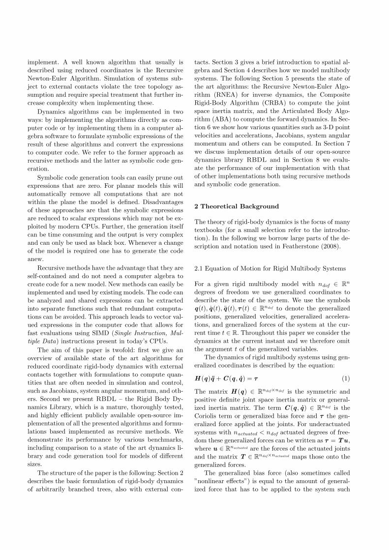
Fig. 2 Performance comparisons of RBDL with Simbodyfor models with increasing numbers of degrees of freedom.All computations were performed on a i7-3770.
plementations are able to reduce computations by eval-
uating articulated body inertias only once. The com-
putations are performed on planar chains of varying
lengths in the range of 5 to 100 degrees of freedom. As
both RBDL and Simbody internally use a 3-D formu-
lation the benchmark generalizes to 3-D models.
For the O(n) forward dynam-
ics comparison we use the method
calcAccelerationsIgnoringConstraints() of
Simbody and ForwardDynamics() of RBDL. Both
libraries have designated operators to solve the ex-
pression H (q)−1τ in O(n) time: in Simbody it is
implemented in multiplyByMInv() and in RBDL it is
called CalcMInvTimesTau(). Both implementations of
this operator allow to efficiently solve the systems for
multiple arguments of τ by evaluating the articulated
body inertias only once. This is exploited in Simbody
in the function MInv() that computes the inverse of
the joint space inertia matrix. RBDL does not contain
a specific function to compute H (q)−1 but we imple-
mented a similar function as in Simbody specifically
for the benchmark in this paper. All computations
were performed in three batches of 100.000 evaluations.
The fastest batch was used to create a data point in
the plots shown in Figure 2.
The top plot shows the comparison of the O(n)
forward dynamics computation. Both implementations
show as expected a linear increase of computation time
when increasing the numbers of degrees of freedom of
the benchmark model. The data points of RBDL are
consistently below those of Simbody. For a model with
35 degrees of freedom RBDL uses on average 12.75µs
for the forward dynamics whereas it takes 21.71µs us-
ing Simbody. Overall RBDL is around 38% faster than
Simbody for the O(n) forward dynamics computations.
The second plot compares the computation times
for the H (q)−1τ solution operator when calling it for
a single vector of generalized torques τ . Similarly as the
previous comparison one can see the linear algorithmic
complexity of both implementations and again RBDL
is consistently faster than Simbody. The difference here
is not as dramatic as before and RBDL is around 15%
faster than Simbody. We assume that more optimiza-
tion went into this routine for Simbody as the library
makes use of this function when simulating constrained
systems.
In the bottom plot we compare multiple invocations
of the solution operator for M−1τ where the articu-
lated body inertias IA are only computed once and
reused in subsequent calls. Again RBDL shows better
performance albeit being here only around 9%.

Overall benchmarks show that RBDL performs
very well compared to a well established dynamics code
such as Simbody.
8.3 Comparison with Symbolic Code Generation
We evaluated the performance of RBDL with
symbolically generated code. that compute
H (q),C (q , q),G(q), and γ(q , q) for the humanoid
robot model with 35 degrees of freedom that we
already used in Section 8.1. One should note that the
computational efforts of C (q , q) is only dependent on
the number of degrees of freedom, however for H (q)
also the structure of the robot is relevant. E.g. the
pendulum used in the previous section results in a
dense matrix, whereas a tree structured model, such as
the humanoid model will have zeros at specific entries
of the matrix.
The generated code was produced with the symbolic
code generation tool DYNAMOD that was developed
in our research group and is implemented in Maple �. It
uses the same algorithms as above to construct expres-
sions and generate code for H (q),C (q , q), etc. DY-
NAMOD also caches expressions for every line of the
algorithms. This was required as we experienced crash-
ing of the computer algebra software when generating
code for complex models. We assume that the generated
symbolic equations became too large as we observed ex-
cessive memory usage of the software. Another benefit
of the caching is that it it allows to avoid calculations
of redundant computations, e.g. the expression of f i in
Algorithm 1 is only evaluated once and then reuses its
value. This results in more compact and faster code. At
the time of writing DYNAMOD has not been made
available publicly but is planned for the near future.
For the computations with RBDL used two vari-
ants: one in which it simply computes the values and
the other in which it reuses precomputed values as de-
scribed in Section 7.4. We assessed the performance
when evaluating the quantities required for contact dy-
namics using RBDL and compare it to the performance
of generated C code. For this both RBDL and DY-
NAMOD compute the 6-D contact Jacobian G(q) and
6-D contact Hessian γ(q , q) expressed at the origin of
the constrained bodies. For the benchmark model these
are the bodies labeled RLEG LINK6 and LLEG LINK6
which represent the bodies of the right and left foot. To
formulate for constraints expressed at other points on
these bodies one can use spatial transformations from
Section 3.1.3.
The results of the benchmark are shown in Figure 3
where evaluations of the respective functions have been
performed one million times on PC running Ubuntu
H (q) C (q , q) G(q) γ(q , q) EoMSetup
EoM ContactSetup
0
2
4
6
8
10
12
14
Dur
atio
nfo
r1.0
00.0
00ca
lls(s
)
RBDL Multi-DOF vs Generated
RBDLRBDL (reuse)Generated
Fig. 3 Comparisons for the evaluation of quantities of theequation of motion for RBDL multi-DOF model without andwith reusing of computed values and the equivalent compu-tations performed by generated C code.
14.04 on a Intel i7-3770 processor with 16 GB RAM.
The vertical axis represents the duration in seconds,
whereas the different function evaluations are listed on
the horizontal axis. The last two groups of bar plots
with the labels ”EoM Setup” and ”EoM Contact Setup”
are benchmarks for computing all quantities to con-
struct the linear systems of Equation (1) and Equation
(7) respectively by reusing as many computations as
possible. Please note that this benchmark does not in-
clude the time required to actually solve these systems,
instead it only is concerned on the computation on the
required quantities.
Overall one can see that evaluation using symbol-ically generated code is faster when values are not
reused. However if values can be reused the recursive
methods can reach the efficiency of generated code, such
as for the computation of H (q) where RBDL needs
6.76s, the reuse variant 4.42s, and the generated code
5.49s. For the evaluation of C (q , q) unfortunately no
computations can be saved and the generated code is
with 2.94s almost twice as fast as the 5.25s of RBDL.
Reusing of computed values is particularly beneficial for
G(q) and γ(q , q). For the former RBDL needs 5.57s
and 1.15s when reusing values, it comes close to the
evaluation of the generated code which used 0.90s. The
evaluation of the contact Hessian is particularly fast for
the reusing RBDL variant: it needs 0.01s, compared to
the non-reusing 7.72s and the 0.77s for the generated
code. This is due to the specific choice of the coordinate
system for which the Hessian is expressed: it is simply
a i when q = 0. Therefore no computations have to be
made and the durations are simply due to the copy-
ing of the values. Computations of H (q) and C (q , q)

while reusing the values amounts to 9.54s for RBDL
and 8.52s for the generated code which makes it about
13% faster. The evaluation of the quantities required for
contact dynamics takes 10.91s for RBDL when reusing
values and 10.21s for the generated code. Here the ad-
vantage of generated code is reduced to about 7%. In
the case of computing the forward dynamics these num-
bers roughly half as factorizations of the linear system
will consume a large portion of the computation time.
One interesting observation here is that the sum of
the timings for the individual quantities is less than the
timings for ”EoM Contact Setup”. This is probably due
to effects related to the instruction cache of the CPU.
For the benchmarks of the individual quantities we run
the specific functions over and over whereas for ”EoM
Setup” and ”EoM Contact Setup” we repeatedly first
compute C (q , q), then H (q) and then the contact Ja-
cobians and Hessians if required. This results in larger
reading and writing to a larger range of memory which
has to be retrieved from slower memory hierarchies.
The comparisons show that faster code can be ob-
tained when using a symbolic code generation ap-
proach. However in practical situations the performance
of RBDL is likely to be better as the Jacobians and
Hessians can also be evaluated for only one foot. The
code generation approach used here always evaluates
the Jacobians and Hessians for all bodies. One might
suggest to generate code for each body individually,
however this will increase the number of redundant
computations as the Jacobians of the bodies share ex-
pressions.
9 Conclusion and Outlook
In this paper we have given an introduction into the
equations related to rigid body dynamics together with
the formulation of the dynamics using spatial algebra.
We have summarized some of the most efficient and
powerful algorithms for generalized coordinate formu-
lations of multibody systems along with a complete de-
scription of a model for any loop free rigid multibody
system. We have shown how other quantities, such as
Jacobians, linear point velocities and accelerations, sys-
tem angular momentum, and others can be expressed
using the model description. We have described how
structures occurring in spatial algebra can be exploited
and how computations can be reused to accomplish fur-
ther performance gains. A performance comparison of
RBDL with a state of the art rigid multibody dynamics
libraries based on recursive methods and code genera-
tion library was given for models of varying sizes.
The comparisons show that the performance our im-
plementation of recursive methods is faster than that
of the well established Simbody library. The compar-
ison of RBDL with symbolic code generation indicate
that the latter is faster, however one should not under-
estimate the ease of use of recursive methods used in
RBDL and their independence of a separate code gen-
eration step. Also the flexibility of recursive methods
in terms of extension, selective evaluation, and model
modification during runtime likely outweigh the small
performance increase of the generated code.
For future work we plan to extend the implemented
contact formulation to allow unilateral contacts and
friction. Another area of work is to expose the compu-
tations of RBDL to other computational environments
such as Matlab� and Python.
Acknowledgements The author gratefully acknowledgesthe financial support and the inspiring environment providedby the Heidelberg Graduate School of Mathematical andComputational Methods for the Sciences, funded by DFG(Deutsche Forschungsgemeinschaft) and the support by theEuropean Commission under the FP7 projects ECHORD(grant number 231143) and Koroibot (grant number 611909).
The author furthermore wants to thank Katja Mombaurfor the opportunity to work in the stimulating environmentof her research group Optimization in Robotics and Biome-chanics and to Henning Koch for creating the generated codeusing his powerful DYNAMOD package.
References
Armstrong WW (1979) Recursive solution to the equa-
tions of motion of an n-link manipulator. In: Proc.
5th World Congress on Theory of Machines and
Mechanisms, pp 1343–1346 1
Ascher UM, Chin H, Petzold LR, Reich S (1994) Stabi-
lization of constrained mechanical systems with daes
and invariant manifolds. J Mech Struct Machines
23:135–157 3
Ball RS (1900) A Treatise on the Theory of Screws.
Cambridge University Press 1
Craig J (2005) Introduction to Robotics: Mechanics and
Control. Addison-Wesley series in electrical and com-
puter engineering: control engineering, Pearson Edu-
cation, Incorporated 1
Featherstone R (1983) The calculation of robot dy-
namics using articulated-body inertias. The Interna-
tional Journal of Robotics Research 2(1):13–30, DOI
10.1177/027836498300200102 1, 9
Featherstone R (2001) The acceleration vector
of a rigid body. The International Journal of
Robotics Research 20(11):841–846, DOI 10.1177/
02783640122068137 5
Featherstone R (2006) Plucker basis vectors. In: ICRA,
pp 1892–1897, DOI 10.1109/ROBOT.2006.1641982 4

Featherstone R (2008) Rigid Body Dynamics Algo-
rithms. Springer 2, 6, 8, 9, 12, 13
Featherstone R (2010) A beginner’s guide to 6-d vec-
tors (part 1). Robotics Automation Magazine, IEEE
17(3):83–94, DOI 10.1109/MRA.2010.937853 4
Featherstone R, Orin D (2000) Robot dynamics: equa-
tions and algorithms. In: Robotics and Automa-
tion (ICRA), 2000. Proceedings of IEEE Interna-
tional Conference on, vol 1, pp 826–834 vol.1, DOI
10.1109/ROBOT.2000.844153 1
Guennebaud G, Jacob B, et al (2010) Eigen v3.
http://eigen.tuxfamily.org 11
Jain A (1991) Unified formulation of dynamics for se-
rial rigid multibody systems. Journal of Guidance,
Control, and Dynamics 14(3):531–542, DOI 10.2514/
3.20672 9
Jain A (2011) Robot and Multibody Dynamics.
Springer US, DOI 10.1007/978-1-4419-7267-5 1
Jain A, Rodriguez G (1993) An analysis of the kine-
matics and dynamics of underactuated manipula-
tors. Robotics and Automation, IEEE Transactions
on 9(4):411–422, DOI 10.1109/70.246052 1
Kanehiro F, Hirukawa H, Kajita S (2004) OpenHRP:
Open architecture humanoid robotics platform.
The International Journal of Robotics Research
23(2):155–165, DOI 10.1177/0278364904041324 14
Khalil W, Dombre E (2004) Modeling, Identification
and Control of Robots. Kogan Page Science paper
edition, Elsevier Science 1
Luh JYS, Walker MW, Paul RPC (1980) On-line
computational scheme for mechanical manipulators.
Journal of Dynamic Systems, Measurement, and
Control 102:69–102, DOI 10.1115/1.3149599 1
Orin D, Goswami A (2008) Centroidal momentum ma-
trix of a humanoid robot: Structure and properties.
In: Intelligent Robots and Systems, 2008. IROS 2008.
IEEE/RSJ International Conference on, pp 653–659,
DOI 10.1109/IROS.2008.4650772 11
Pang JS, Trinkle JC (1996) Complementarity formu-
lations and existence of solutions of dynamic multi-
rigid-body contact problems with coulomb friction.
Mathematical Programming 73(2):199–226, DOI 10.
1007/BF02592103 3
Pfeiffer F, Glocker C (2008) Multibody Dynamics with
Unilateral Contacts. Wiley Series in Nonlinear Sci-
ence, Wiley 3
Rodriguez G (1987) Kalman filtering, smoothing, and
recursive robot arm forward and inverse dynamics.
Robotics and Automation, IEEE Journal of 3(6):624–
639, DOI 10.1109/JRA.1987.1087147 1
Rodriguez G, Kreutz K, Milman M (1988) A spa-
tial operator algebra for manipulator modeling and
control. In: Intelligent Control, 1988. Proceedings.,
IEEE International Symposium on, pp 418–423, DOI
10.1109/ISIC.1988.65468 1
Rodriguez G, Jain A, Kreutz-Delgado K (1991) A spa-
tial operator algebra for manipulator modeling and
control. The International Journal of Robotics Re-
search 10(4):371–381 14
Sherman MA, Seth A, Delp SL (2011) Simbody: multi-
body dynamics for biomedical research. Procedia IU-
TAM 2(0):241 – 261, DOI 10.1016/j.piutam.2011.04.
023, IUTAM Symposium on Human Body Dynamics
14
Shoemake K (1985) Animating rotation with quater-
nion curves. In: Proceedings of the 12th Annual Con-
ference on Computer Graphics and Interactive Tech-
niques, ACM, New York, NY, USA, SIGGRAPH ’85,
pp 245–254, DOI 10.1145/325334.325242 8
Uchida TK, Sherman MA, Delp SL (2015) Making a
meaningful impact: modelling simultaneous frictional
collisions in spatial multibody systems. Proceedings
of the Royal Society of London A: Mathematical,
Physical and Engineering Sciences 471(2177), DOI
10.1098/rspa.2014.0859 3
Recommended