Optimization Techniques For Queries with Expensive
Methods
JOSEPH M. HELLERSTEIN
U.C. Berkeley
Object-Relational database management systems allow knowledgeable users to de�ne new data
types, as well as new methods (operators) for the types. This exibility produces an attendant
complexity, which must be handled in new ways for an Object-Relational database management
system to be e�cient.
In this paper we study techniques for optimizing queries that contain time-consumingmethods.
The focus of traditional query optimizers has been on the choice of join methods and orders;
selections have been handled by \pushdown" rules. These rules apply selections in an arbitrary
order before as many joins as possible, using the assumption that selection takes no time. However,
users of Object-Relational systems can embed complexmethods in selections. Thus selections may
take signi�cant amounts of time, and the query optimization model must be enhanced.
In this paper, we carefully de�ne a query cost framework that incorporates both selectivity and
cost estimates for selections. We developan algorithmcalledPredicate Migration, and prove that it
produces optimal plans for queries with expensive methods. We then describe our implementation
of PredicateMigration in the commercialObject-Relationaldatabasemanagement system Illustra,
and discuss practical issues that a�ect our earlier assumptions. We compare Predicate Migration
to a variety of simpler optimization techniques, and demonstrate that Predicate Migration is the
best general solution to date. The alternative techniques we present may be useful for constrained
workloads.
Categories and Subject Descriptors: H.2.4 [Database Management]: Systems|Query Process-
ing
General Terms: Query Optimization, Expensive Methods
Additional Key Words and Phrases: Object-Relational databases, extensibility, Predicate Migra-
tion, predicate placement
Preliminary versions of this work appeared in Proceedings ACM-SIGMOD International Con-
ference on Management of Data, 1993 and 1994. This work was funded in part by a National
Science FoundationGraduate Fellowship. Any opinions, �ndings, conclusions or recommendations
expressed in this publication are those of the author and do not necessarily re ect the views of the
National Science Foundation. This work was also funded by NSF grant IRI-9157357. This is a pre-
liminary release of an article accepted by ACM Transactions on Database Systems. The de�nitive
version is currently in production at ACM and, when released, will supersede this version.
Address: Author's current address: University of California, Berkeley, EECS Computer Science
Division, 387 Soda Hall #1776, Berkeley, California, 94720-1776. Email: [email protected].
Web: http://www.cs.berkeley.edu/~jmh/.
ACM Copyright Notice: Copyright 1997 by the Association for Computing Machinery, Inc.
Permission to make digital or hard copies of part or all of this work for personal or classroomuse is
grantedwithout fee provided that copies are not made or distributed for pro�t or direct commercial
advantage and that copies show this notice on the �rst page or initial screen of a display along
with the full citation. Copyrights for components of this work owned by others than ACM must
be honored. Abstracting with credit is permitted. To copy otherwise, to republish, to post on
servers, to redistribute to lists, or to use any component of this work in other works, requires prior
speci�c permission and/or a fee. Permissions may be requested from Publications Dept, ACM
Inc., 1515 Broadway, New York, NY 10036 USA, fax +1 (212) 869-0481, or [email protected].
2 � J.M. Hellerstein
1. OPENING
One of the major themes of database research over the last 15 years has been the
introduction of extensibility into Database Management Systems (DBMSs). Rela-
tional DBMSs have begun to allow simple user-de�ned data types and functions
to be utilized in ad-hoc queries [Pirahesh 1994]. Simultaneously, Object-Oriented
DBMSs have begun to o�er ad-hoc query facilities, allowing declarative access to
objects and methods that were previously only accessible through hand-coded, im-
perative applications [Cattell 1994]. More recently, Object-Relational DBMSs were
developed to unify these supposedly distinct approaches to data management [Il-
lustra Information Technologies, Inc. 1994; Kim 1993].
Much of the original research in this area focused on enabling technologies, i.e.
system and language designs that make it possible for a DBMS to support extensi-
bility of data types and methods. Considerably less research explored the problem
of making this new functionality e�cient.
This paper addresses a basic e�ciency problem that arises in extensible database
systems. It explores techniques for e�ciently and e�ectively optimizing declara-
tive queries that contain time-consuming methods. Such queries are natural in
modern extensible database systems, which were expressly designed to support
declarative queries over user-de�ned types and methods. Note that \expensive"
time-consuming methods are natural for complex user-de�ned data types, which
are often large objects that encode signi�cant complexity of information (e.g., ar-
rays, images, sound, video, maps, circuits, documents, �ngerprints, etc.) In order to
e�ciently process queries containing expensive methods, new techniques are needed
to handle expensive methods.
1.1 A GIS Example
To illustrate the issues that can arise in processing queries with expensive meth-
ods, consider the following example over the satellite image data presented in the
Sequoia benchmark for Geographic Information Systems (GIS) [Stonebraker et al.
1993]. The query retrieves names of digital \raster" images taken by a satellite;
particularly, it selects the names of images from the �rst time period of observation
that show a given level of vegetation in over 20% of their pixels:
Example 1.
SELECT name
FROM rasters
WHERE rtime = 1
AND veg(raster) > 20;
In this example, the method veg reads in 16 megabytes of raster image data (infrared
and visual data from a satellite), and counts the percentage of pixels that have the
characteristics of vegetation (these characteristics are computed per pixel using a
standard technique in remote sensing [Frew 1995].) The veg method is very time-
consuming, taking many thousands of instructions and I/O operations to compute.
It should be clear that the query will run faster if the selection rtime = 1 is appliedbefore the veg selection, since doing so minimizes the number of calls to veg. A
traditional optimizer would order these two selections arbitrarily, and might well
Optimization Techniques For Queries with Expensive Methods � 3
apply the veg selection �rst. Some additional logic must be added to the optimizer
to ensure that selections are applied in a judicious order.
While selection ordering such as this is important, correctly ordering selections
within a table-access is not su�cient to solve the general optimization problem of
where to place predicates in a query execution plan. Consider the following example,
which joins the rasters table with a table that contains notes on the rasters:
Example 2.
SELECT rasters.name, notes.note
FROM rasters, notes
WHERE rasters.rtime = notes.rtime
AND notes.author = 'Cli�ord'
AND veg(rasters.raster) > 20;
Traditionally, an optimizer would plan this query by applying all the single-table
selections in the WHERE clause before performing the join of rasters and notes. Thisheuristic, often called \predicate pushdown", is considered bene�cial since early
selections usually lower the complexity of join processing, and are traditionally
considered to be trivial to check [Palermo 1974]. However in this example the cost
of evaluating the expensive selection predicate may outweigh the bene�t gained by
doing selection before join. In other words, this may be a case where predicate
pushdown is precisely the wrong technique. What is needed here is \predicate
pullup", namely postponing the time-consuming selection veg(rasters.raster) > 20until after computing the join of rasters and notes.In general it is not clear how joins and selections should be interleaved in an opti-
mal execution plan, nor is it clear whether the migration of selections should have an
e�ect on the join orders and methods used in the plan. We explore these query opti-
mization problems from both a theoretical point of view, and from the experience of
producing an industrial-strength implementation for the Illustra Object-Relational
DBMS.
1.2 Bene�ts for RDBMS: Subqueries
It is important to note that expensive methods do not exist only in next-generation
Object-Relational DBMSs. Current relational languages, such as the industry stan-
dard, SQL [ISO ANSI 1993], have long supported expensive predicate methods in
the guise of subquery predicates. A subquery predicate is one of the form expres-
sion operator query. Evaluating such a predicate requires executing an arbitrary
query and scanning its result for matches | an operation that is arbitrarily expen-
sive, depending on the complexity and size of the subquery. While some subquery
predicates can be converted into joins (thereby becoming subject to traditional
join-based optimization and execution strategies) even sophisticated SQL rewrite
systems such as that of DB2/CS [Pirahesh et al. 1992; Seshadri et al. 1996; Seshadri
et al. 1996] cannot convert all subqueries to joins. When one is forced to compute
a subquery in order to evaluate a predicate, then the predicate should be treated
as an expensive method. Thus the work presented in this paper is applicable to
the majority of today's production RDBMSs, which support SQL subqueries but
do not intelligently place subquery predicates in a query plan.
4 � J.M. Hellerstein
1.3 Outline
Chapter 2 presents the theoretical underpinnings of Predicate Migration, an algo-
rithm to optimally place expensive predicates in a query plan. Chapter 3 discusses
three simpler alternatives to Predicate Migration, and uses performance of queries
in Illustra to demonstrate the situations in which each technique works. Chapter 4
discusses related work in the research literature. Concluding remarks and directions
for future research appear in Chapter 5.
1.4 Environment for Experiments
In the course of the paper we will examine the behavior of various algorithms via
both analysis and experiments. All the experiments presented in the paper were
run in the commercial Object-Relational DBMS Illustra. A development version
of Illustra was used, similar to the publicly released version 2.4.1. Except when
otherwise noted, Illustra was run with its default con�guration, with the exception
of settings to produce traces of query plans and execution times. The machine used
was a Sun Sparcstation 10/51 with 2 processors and 64 megabytes of RAM, running
SunOS Release 4.1.3. One Seagate 2.1-gigabyte SCSI disk (model #ST12400N) was
used to hold the databases. The binaries for Illustra were stored on an identical Sea-
gate 2.1-gigabyte SCSI disk, Illustra's logs were stored on a Seagate 1.05-gigabyte
SCSI disk (model #ST31200N), and 139 megabytes of swap space was allocated on
another Seagate 1.05-gigabyte SCSI disk (model #ST31200N).
Due to restrictions from Illustra Information Technologies, most of the perfor-
mance numbers presented in the paper are relative rather than absolute: the graphs
are scaled so that the lowest data point has the value 1.0. Unfortunately, commercial
database systems typically have a clause in their license agreements that prohibits
the release of performance numbers. It is unusual for a database vendor to permit
publication of any performance results at all, relative or otherwise [Carey et al.
1994]. The scaling of results in this paper does not a�ect the conclusions drawn
from the experiments, which are based on the relative performance of various ap-
proaches.
2. A THEORETICAL BASIS
In general it is not clear how joins and selections should be interleaved in an opti-
mal execution plan, nor is it clear whether the migration of selections should have
an e�ect on the join orders and methods used in the plan. This section describes
and proves the correctness of the Predicate Migration Algorithm, which produces
an optimal query plan for queries with expensive predicates. Predicate Migration
modestly increases query optimization time: the additional cost factor is polyno-
mial in the number of operators in a query plan. This compares favorably to the
exponential join enumeration schemes used by standard query optimizers, and is
easily circumvented when optimizing queries without expensive predicates | if
no expensive predicates are found while parsing the query, the techniques of this
section need not be invoked. For queries with expensive predicates, the gains in
execution speed should o�set the extra optimization time. We have implemented
Predicate Migration in Illustra, integrating it with Illustra's standard System R-
style optimizer [Selinger et al. 1979]. With modest overhead in optimization time,
Optimization Techniques For Queries with Expensive Methods � 5
Predicate Migration can reduce the execution time of many practical queries by
orders of magnitude. This is illustrated further below.
2.1 Background: Optimizer Estimates
To develop our optimizations, we must enhance the traditional model for analyzing
query plan cost. This will involve some modi�cation of the usual metrics for the
expense and selectivity of relational operators. This preliminary discussion of our
model will prove critical to the analysis below.
A relational query in a language such as SQL may have a WHERE clause, which
contains an arbitrary Boolean expression over constants and the range variables of
the query. We break such clauses into a maximal set of conjuncts, or \Boolean
factors" [Selinger et al. 1979], and refer to each Boolean factor as a distinct \pred-
icate" to be satis�ed by each result tuple of the query. When we use the term
\predicate" below, we refer to a Boolean factor of the query's where clause. A join
predicate is one that refers to multiple tables, while a selection predicate refers only
to a single table.
2.1.1 Selectivity. Traditional query optimizers compute selectivities for both joins
and selections. That is, for any predicate p (join or selection) they estimate the
value
selectivity(p) =cardinality(output(p))
cardinality(input(p)):
Typically these estimations are based on default values and statistics stored by the
DBMS [Selinger et al. 1979], although recent work suggests that inexpensive sam-
pling techniques can be used [Lipton et al. 1993; Hou et al. 1988; Haas et al. 1995].
Accurate selectivity estimation is a di�cult problem in query optimization, and has
generated increasing interest in recent years [Ioannidis and Christodoulakis 1991;
Faloutsos and Kamel 1994; Ioannidis and Poosala 1995; Poosala et al. 1996; Poosala
and Ioannidis 1996]. In Illustra, selectivity estimation for user-de�ned methods can
be controlled through the selfunc ag of the create function command [Illustra
Information Technologies, Inc. 1994]. In this paper we make the standard assump-
tions of most query optimization algorithms, namely that estimates are accurate
and predicates have independent selectivities.
2.1.2 Di�erential Cost of User-De�ned Methods. In an extensible system such as
Illustra, arbitrary user-de�ned methods may be introduced into both selection and
join predicates. These methods can be written in a general programming language
such as C, or in a database query language, e.g., SQL. In this section we discuss
programming language methods; we handle query language methods and subqueries
in Section 2.1.3.
Given that user-de�ned methods may be written in a general purpose language
such as C, it is di�cult for the database to correctly estimate the cost of predicates
containing these methods, at least initially.1 As a result, Illustra includes syntax
1After repeated applications of a method, one could collect performance statistics and use curve-
�tting techniques to make estimates about the method's behavior| see for example [Boulos et al.
1997].
6 � J.M. Hellerstein
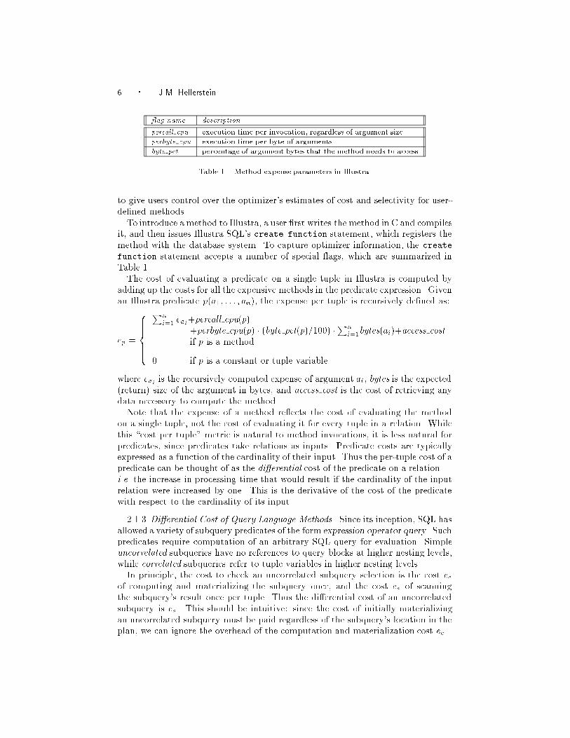
ag name description
percall cpu execution time per invocation, regardless of argument size
perbyte cpu execution time per byte of arguments
byte pct percentage of argument bytes that the method needs to access
Table 1. Method expense parameters in Illustra.
to give users control over the optimizer's estimates of cost and selectivity for user-
de�ned methods.
To introduce a method to Illustra, a user �rst writes the method in C and compiles
it, and then issues Illustra SQL's create function statement, which registers the
method with the database system. To capture optimizer information, the create
function statement accepts a number of special ags, which are summarized in
Table 1.
The cost of evaluating a predicate on a single tuple in Illustra is computed by
adding up the costs for all the expensive methods in the predicate expression. Given
an Illustra predicate p(a1; : : : ; an), the expense per tuple is recursively de�ned as:
ep =
8>>><>>>:
Pn
i=1 eai+percall cpu(p)
+perbyte cpu(p) � (byte pct(p)=100) �Pn
i=1bytes(ai)+access cost
if p is a method
0 if p is a constant or tuple variable
where eai is the recursively computed expense of argument ai, bytes is the expected
(return) size of the argument in bytes, and access cost is the cost of retrieving any
data necessary to compute the method.
Note that the expense of a method re ects the cost of evaluating the method
on a single tuple, not the cost of evaluating it for every tuple in a relation. While
this \cost per tuple" metric is natural to method invocations, it is less natural for
predicates, since predicates take relations as inputs. Predicate costs are typically
expressed as a function of the cardinality of their input. Thus the per-tuple cost of a
predicate can be thought of as the di�erential cost of the predicate on a relation |
i.e. the increase in processing time that would result if the cardinality of the input
relation were increased by one. This is the derivative of the cost of the predicate
with respect to the cardinality of its input.
2.1.3 Di�erential Cost of Query Language Methods. Since its inception, SQL has
allowed a variety of subquery predicates of the form expression operator query. Such
predicates require computation of an arbitrary SQL query for evaluation. Simple
uncorrelated subqueries have no references to query blocks at higher nesting levels,
while correlated subqueries refer to tuple variables in higher nesting levels.
In principle, the cost to check an uncorrelated subquery selection is the cost ecof computing and materializing the subquery once, and the cost es of scanning
the subquery's result once per tuple. Thus the di�erential cost of an uncorrelated
subquery is es. This should be intuitive: since the cost of initially materializing
an uncorrelated subquery must be paid regardless of the subquery's location in the
plan, we can ignore the overhead of the computation and materialization cost ec.
Optimization Techniques For Queries with Expensive Methods � 7
Correlated subqueries must be recomputed for each tuple that is checked against
the subquery predicate, and hence the di�erential cost for correlated subqueries is
ec. We ignore es here since scanning can be done during each recomputation, and
does not represent a separate cost. Illustra also allows for user-de�ned methods
that can be written in SQL; these are essentially named, correlated subqueries.
The cost estimates presented here for query language methods form a simple
model and raise some issues in setting costs for subqueries. The cost of a subquery
predicate may be lowered by transforming it to another subquery predicate [Lohman
et al. 1984], and by \early stop" techniques, which stop materializing or scanning a
subquery as soon as the predicate can be resolved [Dayal 1987]. Incorporating such
schemes is beyond the scope of this paper, but including them into the framework of
the later sections merely requires more careful estimates of the di�erential subquery
costs.
2.1.4 Estimates for Joins. In our subsequent analysis, we will be treating joins
and selections uniformly in order to optimally balance their costs and bene�ts. In
order to do this, we will need to measure the expense of a join per tuple of each
of the join's inputs; that is, we need to estimate the di�erential cost of the join
with respect to each input. We are given a join algorithm over outer relation R and
inner relation S, with cost function f(jRj; jSj), where jRj and jSj are the numbers of
tuples in R and S respectively. From this information, we compute the di�erential
cost of the join with respect to its outer relation as @f@jRj ; the di�erential cost of the
join with respect to its inner relation is @f
@jSj. We will see in Section 3 that these
partial di�erentials are constants for all the well-known join algorithms, and hence
the cost of a join per tuple of each input is typically well de�ned and independent
of the cardinality of either input.
We also need to characterize the selectivity of a join with respect to each of
its inputs. Traditional selectivity estimation [Selinger et al. 1979] computes the
selectivity sJ of a join J of relations R and S as the expected number of tuples in
the output of J (OJ ) over the number of tuples in the Cartesian product of the input
relations, i.e., sJ = jOJ j=jR�Sj = jOJ j=(jRj � jSj). The selectivity sJ(R) of the join
with respect to R can be derived from the traditional estimation: it is the size of
the output of the join relative to the size of R, i.e., sJ(R) = jOJ j=jRj= sJ � jSj. The
selectivity sJ(S) with respect to S is derived similarly as sJ(S) = jOJ j=jSj = sJ � jRj.
Note that a query may contain multiple join predicates over the same set of
relations. In an execution plan for a query, some of these predicates are used in
processing a join, and we call these primary join predicates. Merge join, hash join,
and index nested-loop join all have primary join predicates implicit in their pro-
cessing. Join predicates that are not applicable in processing the join are merely
used to select from its output, and we refer to these as secondary join predicates.
Secondary join predicates are essentially no di�erent from selection predicates, and
we treat them as such. These predicates may then be reordered and even pulled up
above higher join nodes, just like selection predicates. Note, however, that a sec-
ondary join predicate must remain above its corresponding primary join. Otherwise
the secondary join predicate would be impossible to evaluate.2
2Nested-loop join without an index is essentially a Cartesian product followed by selection, but
8 � J.M. Hellerstein
2.2 Optimal Plans for Queries With Expensive Predicates
At �rst glance, the task of correctly optimizing queries containing expensive pred-
icates appears exceedingly complex. Traditional query optimizers already search
a plan space that is exponential in the number of relations being joined; multi-
plying this plan space by the number of permutations of the selection predicates
could make traditional plan enumeration techniques prohibitively expensive. In
this section we prove the reassuring results that:
(1) Given a particular query plan, its selection predicates can be optimally inter-
leaved based on a simple sorting algorithm.
(2) As a result of the previous point, we need merely enhance the traditional join
plan enumeration with techniques to interleave the predicates of each plan
appropriately. This interleaving takes time that is polynomial in the number
of operators in a plan.
2.2.1 Optimal Predicate Ordering in Table Accesses. We begin our discussion by
focusing on the simple case of queries over a single table. Such queries can have
an arbitrary number of selection predicates, each of which may be a complicated
Boolean function over the table's range variables, possibly containing expensive
subqueries or user-de�ned methods. Our task is to order these predicates in such
a way as to minimize the expense of applying them to the tuples of the relation
being scanned.
If the access path for the query is an index scan, then all the predicates that
match the index and can be satis�ed during the scan are applied �rst. This is
because such predicates have essentially zero cost: they are not actually evaluated,
rather the indices are traversed to retrieve only those tuples that qualify.3 We will
represent the subsequent non-index predicates as p1; : : : ; pn, where the subscript of
the predicate represents its place in the order in which the predicates are applied to
each tuple of the base table. We represent the (di�erential) expense of a predicate pias epi , and its selectivity as spi . Assuming the independence of distinct predicates,
the cost of applying all the non-index predicates to the output of a scan containing
t tuples is
e = ep1t + sp1ep2 t+ : : :+ sp1sp2 � � �spn�1 epn t:
The following lemma demonstrates that this cost can be minimized by a simple
sort on the predicates. It is analogous to the Least-Cost Fault Detection problem
addressed by Monma and Sidney [Monma and Sidney 1979].
Lemma 1. The cost of applying expensive selection predicates to a set of tuples
is minimized by applying the predicates in ascending order of the metric
rank =selectivity� 1
di�erential cost
inexpensive predicates on an unindexed nested-loop join may be considered primary join predi-
cates, since they will not be pulled up. All expensive join predicates are considered secondary,
since they are not essential to the join method and may be pulled up in the plan.3It is possible to index tables on method values as well as on table attributes [Maier and Stein
1986; Lynch and Stonebraker 1988]. If a scan is done on such a \method" index, then predicates
over the method may be satis�ed during the scan without invoking the method. As a result, these
predicates are considered to have zero cost, regardless of the method's expense.
Optimization Techniques For Queries with Expensive Methods � 9
Plan 1
veg(raster) > 50
Select
ScanScan
rasters rasters
Select Select
Select
rtime = 1
veg(raster) > 50
rank = − rank = −0.001
rank = −rank = −0.001
Plan 2(ordered by rank)
rtime = 1
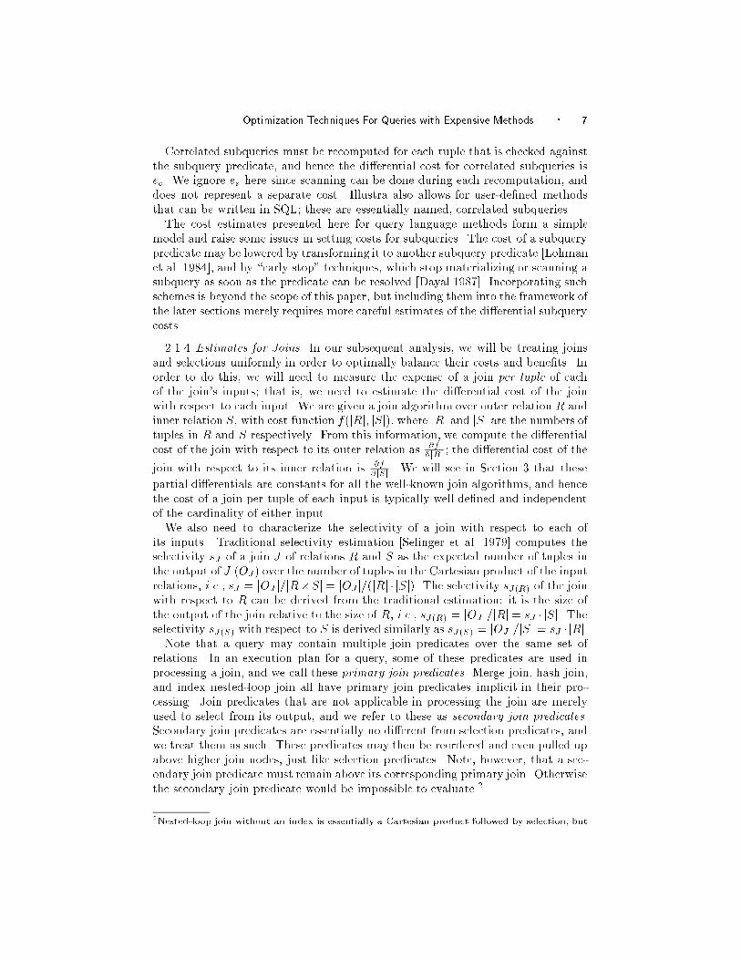
Fig. 1. Two execution plans for Example 1.
Query Plan Optimization Time Execution Time
CPU Elapsed CPU Elapsed
Plan 1 0.01 sec 0.02 sec 2 min 18.09 sec 3 min 25.40 sec
Plan 2 0.10 sec 0.10 sec 0 min 0.03 sec 0 min 0.10 sec
Table 2. Performance of plans for Example 1.
Thus we see that for single table queries, predicates can be optimally ordered by
simply sorting them by their rank. Swapping the position of predicates with equal
rank has no e�ect on the cost of the sequence.
To see the e�ects of reordering selections, we return to Example 1 from the
introduction. We ran the query in Illustra without the rank-sort optimization,
generating Plan 1 of Figure 1, and with the rank-sort optimization, generating
Plan 2 of Figure 1. As we expect from Lemma 1, the �rst plan has higher cost than
the second plan, since the second is correctly ordered by rank. The optimization
and execution times were measured for both runs, as illustrated in Table 2. We
see that correctly ordering selections can improve query execution time by orders
of magnitude, even for simple queries of two predicates and one relation.
2.2.2 Predicate Migration: Placing Selections Among Joins. In the previous sec-
tion, we established an optimal ordering for selections. In this section, we explore
the issue of ordering selections among joins. Since we will eventually be applying
our optimization to each plan produced by a typical join-enumerating query opti-
mizer, our model here is that we are given a �xed join plan, and want to minimize
the plan's cost under the constraint that we may not change the order of the joins.
This section develops a polynomial-time algorithm to optimally place selections
and secondary join predicates in a given join plan. In Section 2.5 we show how to
e�ciently integrate this algorithm into a traditional optimizer, so that the optimal
plan is chosen from the space of all possible join orders, join methods, and selection
placements.
2.2.3 De�nitions. The thrust of this section is to handle join predicates in our
ordering scheme in the same way that we handle selection predicates: by having
them participate in an ordering based on rank.
De�nition 1. A plan tree is a tree whose leaves are scan nodes, and whose internal
nodes are either joins or selections. Tuples are produced by scan nodes and ow
10 � J.M. Hellerstein
upwards along the edges of the plan tree.4
Some optimization schemes constrain plan trees to be within a particular class,
such as the left-deep trees, which have scans as the right child of every join. Our
methods will not require this limitation.
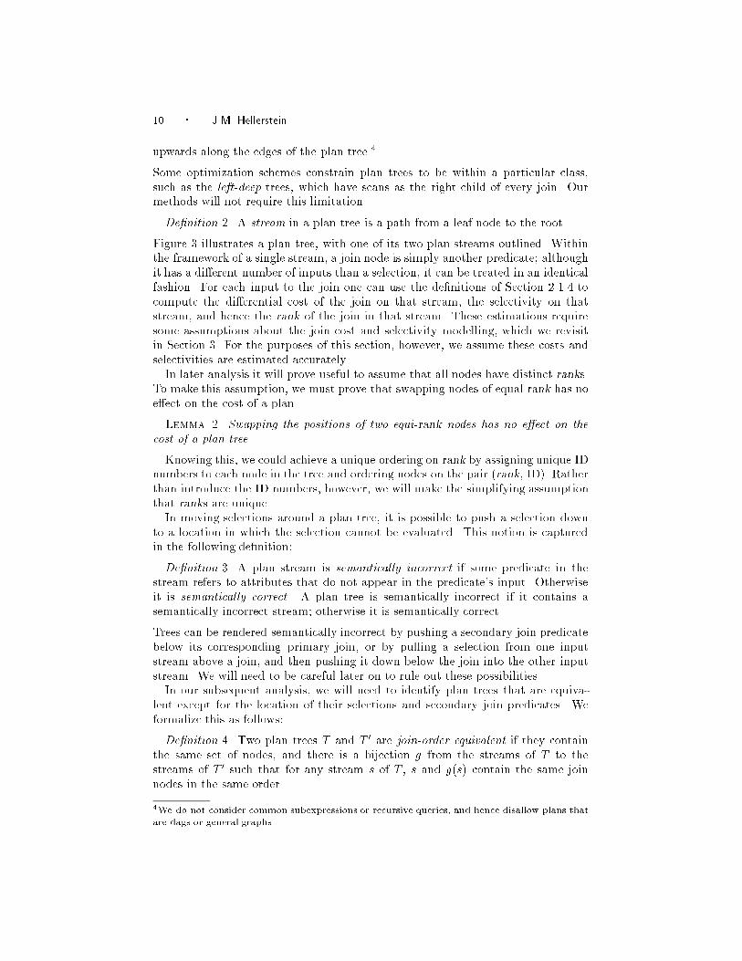
De�nition 2. A stream in a plan tree is a path from a leaf node to the root.
Figure 3 illustrates a plan tree, with one of its two plan streams outlined. Within
the framework of a single stream, a join node is simply another predicate; although
it has a di�erent number of inputs than a selection, it can be treated in an identical
fashion. For each input to the join one can use the de�nitions of Section 2.1.4 to
compute the di�erential cost of the join on that stream, the selectivity on that
stream, and hence the rank of the join in that stream. These estimations require
some assumptions about the join cost and selectivity modelling, which we revisit
in Section 3. For the purposes of this section, however, we assume these costs and
selectivities are estimated accurately.
In later analysis it will prove useful to assume that all nodes have distinct ranks.
To make this assumption, we must prove that swapping nodes of equal rank has no
e�ect on the cost of a plan.
Lemma 2. Swapping the positions of two equi-rank nodes has no e�ect on the
cost of a plan tree.
Knowing this, we could achieve a unique ordering on rank by assigning unique ID
numbers to each node in the tree and ordering nodes on the pair (rank, ID). Rather
than introduce the ID numbers, however, we will make the simplifying assumption
that ranks are unique.
In moving selections around a plan tree, it is possible to push a selection down
to a location in which the selection cannot be evaluated. This notion is captured
in the following de�nition:
De�nition 3. A plan stream is semantically incorrect if some predicate in the
stream refers to attributes that do not appear in the predicate's input. Otherwise
it is semantically correct. A plan tree is semantically incorrect if it contains a
semantically incorrect stream; otherwise it is semantically correct.
Trees can be rendered semantically incorrect by pushing a secondary join predicate
below its corresponding primary join, or by pulling a selection from one input
stream above a join, and then pushing it down below the join into the other input
stream. We will need to be careful later on to rule out these possibilities.
In our subsequent analysis, we will need to identify plan trees that are equiva-
lent except for the location of their selections and secondary join predicates. We
formalize this as follows:
De�nition 4. Two plan trees T and T0 are join-order equivalent if they contain
the same set of nodes, and there is a bijection g from the streams of T to the
streams of T 0 such that for any stream s of T , s and g(s) contain the same join
nodes in the same order.
4We do not consider common subexpressions or recursive queries, and hence disallow plans that
are dags or general graphs.

Optimization Techniques For Queries with Expensive Methods � 11
2.2.4 The Predicate Migration Algorithm: Optimizing a Plan Tree By Optimiz-
ing its Streams. Our approach to optimizing a plan tree will be to treat each of its
streams individually, and sort the nodes in the streams based on their rank. Un-
fortunately, sorting a stream in a general plan tree is not as simple as sorting the
selections in a table access, since the order of nodes in a stream is constrained in two
ways. First, we are not allowed to reorder join nodes, since join-order enumeration
is handled separately from Predicate Migration. Second, we must ensure that each
stream remains semantically correct. In some situations, these constraints may pre-
clude the option of simply ordering a stream by ascending rank, since a predicate
p1 may be constrained to precede a predicate p2, even though rank(p1) > rank(p2).
In such situations, we will need to �nd the optimal ordering of predicates in the
stream subject to the precedence constraints.
Monma and Sidney [Monma and Sidney 1979] have shown that �nding the op-
timal ordering for a single stream under these kinds of precedence constraints can
be done fairly simply. Their analysis is based on two key results:
(1) A set S of plan nodes can be grouped into job modules, where a job module is
de�ned as a subset of nodes S0 � S such that for each element n of S�S0, n has
the same constraint relationship (must precede, must follow, or unconstrained)
with respect to all nodes in S0. An optimal ordering for a job module forms a
subset of an optimal ordering for the entire stream.
(2) For a jobmodule fp1; p2g such that p1 is constrained to precede p2 and rank(p1) >
rank(p2), an optimal ordering will have p1 directly preceding p2, with no other
predicates in between.
Monma and Sidney use these principles to develop the Series-Parallel Algorithm
Using Parallel Chains, an O(n logn) algorithm that can optimize an arbitrarily
constrained stream. The algorithm repeatedly isolates job modules in a stream,
optimizing each job module individually, and using the resulting orders for job
modules to �nd a total order for the stream. We use a version of their algorithm
as a subroutine in our optimization algorithm:
Predicate Migration Algorithm: To optimize a plan tree, push all predicates
down as far as possible, and then repeatedly apply the Series-Parallel Algorithm
Using Parallel Chains [Monma and Sidney 1979] to each stream in the tree, until
no more progress can be made.
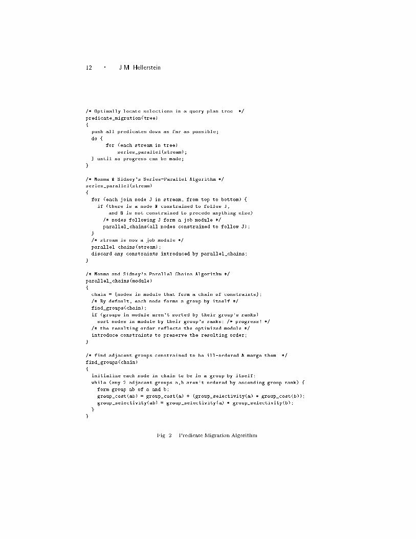
Pseudo-code for the Predicate Migration Algorithm is given in Figure 2, and we
provide a brief explanation of the algorithm here. The constraints in a plan tree
are not general series-parallel constraints, and hence our version of Monma and
Sidney's Series-Parallel Algorithm Using Parallel Chains is somewhat simpli�ed.
The function predicate migration �rst pushes all predicates down as far as
possible. This pre-processing is typically automatic in most System R-style opti-
mizers. The rest of predicate migration is made up of a nested loop. The outer
do loop ensures that the algorithm terminates only when no more progress can be
made (i.e. when all streams are optimally ordered). The inner loop cycles through
all the streams in the plan tree, applying a simple version of Monma and Sidney's
Series-Parallel Algorithm using Parallel Chains.
12 � J.M. Hellerstein
/* Optimally locate selections in a query plan tree. */
predicate_migration(tree)
{
push all predicates down as far as possible;
do {
for (each stream in tree)
series_parallel(stream);
} until no progress can be made;
}
/* Monma & Sidney's Series-Parallel Algorithm */
series_parallel(stream)
{
for (each join node J in stream, from top to bottom) {
if (there is a node N constrained to follow J,
and N is not constrained to precede anything else)
/* nodes following J form a job module */
parallel_chains(all nodes constrained to follow J);
}
/* stream is now a job module */
parallel_chains(stream);
discard any constraints introduced by parallel_chains;
}
/* Monma and Sidney's Parallel Chains Algorithm */
parallel_chains(module)
{
chain = {nodes in module that form a chain of constraints};
/* By default, each node forms a group by itself */
find_groups(chain);
if (groups in module aren't sorted by their group's ranks)
sort nodes in module by their group's ranks; /* progress! */
/* the resulting order reflects the optimized module */
introduce constraints to preserve the resulting order;
}
/* find adjacent groups constrained to be ill-ordered & merge them. */
find_groups(chain)
{
initialize each node in chain to be in a group by itself;
while (any 2 adjacent groups a,b aren't ordered by ascending group rank) {
form group ab of a and b;
group_cost(ab) = group_cost(a) + (group_selectivity(a) * group_cost(b));
group_selectivity(ab) = group_selectivity(a) * group_selectivity(b);
}
}
Fig. 2. Predicate Migration Algorithm.
Optimization Techniques For Queries with Expensive Methods � 13
The series parallel routine traverses the stream from the top down, repeatedly
�nding modules of the stream to optimize. Given a module, it calls parallel -
chains to order the nodes of the module optimally. When parallel chains �nds
the optimal ordering for the module, it introduces constraints to maintain that
ordering as a chain of nodes. Thus series parallel uses the parallel chains
subroutine to convert the stream, from the top down, into a chain. Once the lowest
join node of the stream has been handled by parallel chains, the resulting stream
has a chain of nodes and possibly a set of unconstrained selections at the bottom.
This entire stream is a job module, and parallel chains can be called to optimize
the stream into a single ordering.
Our version of the Parallel Chains algorithm expects as input a set of nodes that
can be partitioned into two subsets: one of nodes that are constrained to form
a chain, and another of nodes that are unconstrained relative to any node in the
entire set. Note that by traversing the stream from the top down, series parallel
always provides correct input to parallel chains.5 The parallel chains routine
�rst �nds groups of nodes in the chain that are constrained to be ordered sub-
optimally (i.e. by descending rank). As shown by Monma and Sidney [Monma
and Sidney 1979], there is always an optimal ordering in which such nodes are
adjacent, and hence such nodes may be considered as an undivided group. The
find groups routine identi�es the maximal-sized groups of poorly-ordered nodes.
After all groups are formed, the module can be sorted by the rank of each group.
The resulting total order of the module is preserved as a chain by introducing
extra constraints. These extra constraints are discarded after the entire stream is
completely ordered.
When predicate migration terminates, it leaves a tree in which each stream has
been ordered by the Series-Parallel Algorithm using Parallel Chains. The interested
reader is referred to [Monma and Sidney 1979] for justi�cation of why the Series-
Parallel Algorithm using Parallel Chains optimally orders a stream.
2.3 Predicate Migration: Proofs of Optimality
Upon termination, the Predicate Migration Algorithm produces a semantically cor-
rect tree in which each stream is well-ordered according to Monma and Sidney; that
is each stream, taken individually, is optimally ordered subject to its precedence
constraints. We proceed to prove that the Predicate Migration Algorithm is guar-
anteed to terminate in polynomial time, and that the resulting tree of well-ordered
streams represents the optimal choice of predicate locations for the entire plan tree.
Lemma 3. Given a join node J in a module, adding a selection or secondary
join predicate R to the stream does not increase the rank of J 's group.
Lemma 4. For any join J and selection or secondary join predicate R in a plan
tree, if the Predicate Migration Algorithm ever places R above J in any stream, it
will never subsequently place J below R.
5Note also that for each module S0 that series parallel constructs from a stream S, each node
of S � S0 is constrained in exactly the same way with respect to each node of S0: every element
of S � S0 is either a primary join predicate constrained to precede all of S0, or a selection or
secondary join predicate that is unconstrained with respect to all of S0. Thus parallel chains is
always passed a valid job module.
14 � J.M. Hellerstein
With Predicate Migration
Join
rtime = rtime
Selectveg(raster) > 50
outer rank = −41.46
rank = −0.001
Without Predicate Migration
Scanrasters
Select
Scan
author = ’Clifford’
notes
rank = −
outer rank = −41.46
Select
Scan
veg(raster) > 50
rasters
Select
Scan
author = ’Clifford’
notes
rank = −0.001
Join
rtime = rtime
rank = −
An unoptimized plan stream
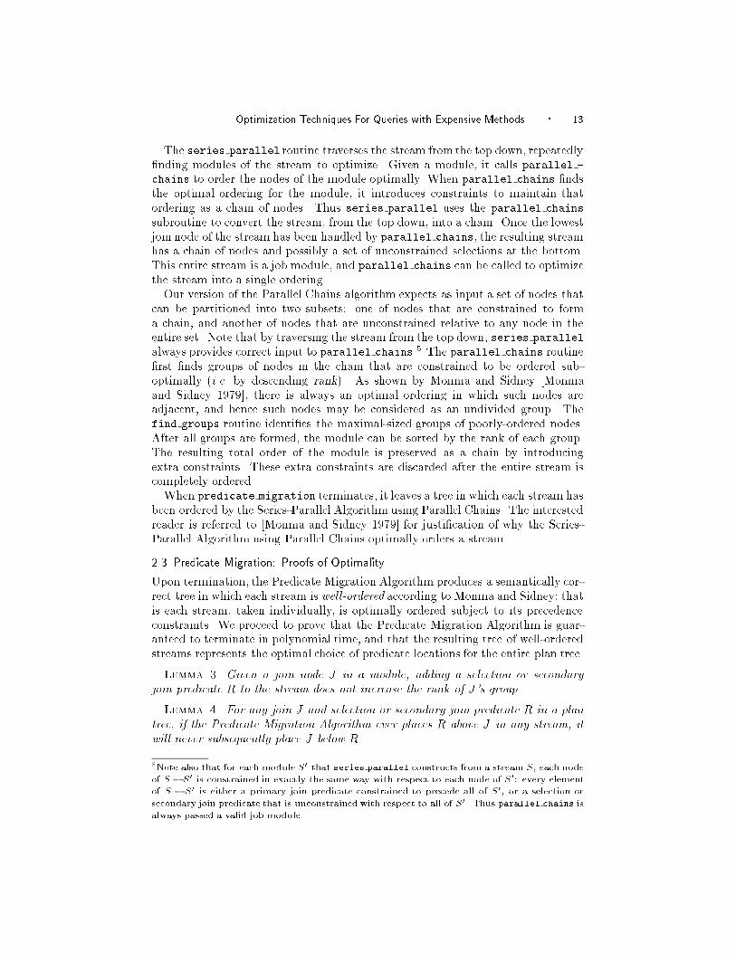
Fig. 3. Plans for Example 2, with and without Predicate Migration.
As a corollary to Lemma 4, we can modify the parallel chains routine: instead
of actually sorting a module, it can simply pull up each selection or secondary
join above as many groups as possible, thus potentially lowering the number of
comparisons in the routine. This optimization is implemented in Illustra.
Theorem 1. Given any plan tree as input, the Predicate Migration Algorithm
is guaranteed to terminate in polynomial time, producing a semantically correct,
join-order equivalent tree in which each stream is well-ordered.
We have now seen that the Predicate Migration Algorithm correctly orders each
stream within a polynomial number of steps. All that remains is to show that the
resulting tree is in fact optimal. We do this by showing that:
(1) There is only one semantically correct tree of well-ordered streams.
(2) Among all semantically correct trees, some tree of well-ordered streams is of
minimum cost.
(3) Since the output of the Predicate Migration Algorithm is the semantically
correct tree of well-ordered streams, it is a minimum cost semantically correct
tree.
Theorem 2. For every plan tree T1 there is a unique semantically correct, join-
order equivalent plan tree T2 with only well-ordered streams. Moreover, among all
semantically correct trees that are join-order equivalent to T1, T2 is of minimum
cost.
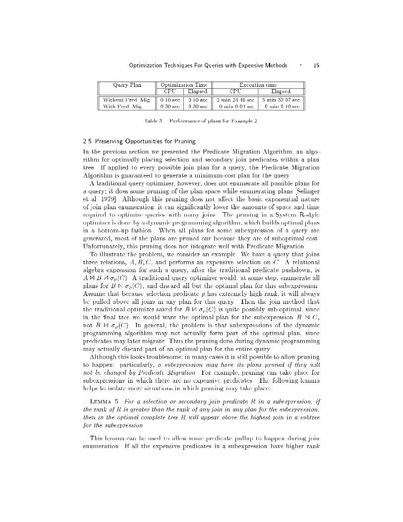
2.4 Example 2 Revisited
Theorems 1 and 2 demonstrate that the Predicate Migration Algorithm produces
our desired minimum-cost interleaving of predicates. As a simple illustration of
the e�cacy of Predicate Migration, we go back to Example 2 from the introduc-
tion. Figure 3 illustrates plans generated for this query by Illustra running both
with and without Predicate Migration. The performance measurements for the two
plans appear in Table 3. It is clear from this example that failure to pull expen-
sive selections above joins can cause performance degradation factors of orders of
magnitude. A more detailed study of placing selections among joins appears in the
next section.
Optimization Techniques For Queries with Expensive Methods � 15
Query Plan Optimization Time Execution time
CPU Elapsed CPU Elapsed
Without Pred. Mig. 0.10 sec 0.10 sec 2 min 24.49 sec 3 min 33.97 sec
With Pred. Mig. 0.30 sec 0.30 sec 0 min 0.04 sec 0 min 0.10 sec
Table 3. Performance of plans for Example 2.
2.5 Preserving Opportunities for Pruning
In the previous section we presented the Predicate Migration Algorithm, an algo-
rithm for optimally placing selection and secondary join predicates within a plan
tree. If applied to every possible join plan for a query, the Predicate Migration
Algorithm is guaranteed to generate a minimum-cost plan for the query.
A traditional query optimizer, however, does not enumerate all possible plans for
a query; it does some pruning of the plan space while enumerating plans [Selinger
et al. 1979]. Although this pruning does not a�ect the basic exponential nature
of join plan enumeration, it can signi�cantly lower the amounts of space and time
required to optimize queries with many joins. The pruning in a System R-style
optimizer is done by a dynamic programming algorithm, which builds optimal plans
in a bottom-up fashion. When all plans for some subexpression of a query are
generated, most of the plans are pruned out because they are of suboptimal cost.
Unfortunately, this pruning does not integrate well with Predicate Migration.
To illustrate the problem, we consider an example. We have a query that joins
three relations, A;B;C, and performs an expensive selection on C. A relational
algebra expression for such a query, after the traditional predicate pushdown, is
A 1 B 1 �p(C). A traditional query optimizer would, at some step, enumerate all
plans for B 1 �p(C), and discard all but the optimal plan for this subexpression.
Assume that because selection predicate p has extremely high rank, it will always
be pulled above all joins in any plan for this query. Then the join method that
the traditional optimizer saved for B 1 �p(C) is quite possibly sub-optimal, since
in the �nal tree we would want the optimal plan for the subexpression B 1 C,
not B 1 �p(C). In general, the problem is that subexpressions of the dynamic
programming algorithm may not actually form part of the optimal plan, since
predicates may later migrate. Thus the pruning done during dynamic programming
may actually discard part of an optimal plan for the entire query.
Although this looks troublesome, in many cases it is still possible to allow pruning
to happen: particularly, a subexpression may have its plans pruned if they will
not be changed by Predicate Migration. For example, pruning can take place for
subexpressions in which there are no expensive predicates. The following lemma
helps to isolate more situations in which pruning may take place:
Lemma 5. For a selection or secondary join predicate R in a subexpression, if
the rank of R is greater than the rank of any join in any plan for the subexpression,
then in the optimal complete tree R will appear above the highest join in a subtree
for the subexpression.
This lemma can be used to allow some predicate pullup to happen during join
enumeration. If all the expensive predicates in a subexpression have higher rank
16 � J.M. Hellerstein
than any join in any subtree for the subexpression, then the expensive predicates
may be pulled to the top of the subtrees, and the subexpression without the ex-
pensive predicates may be pruned as usual. As an example, we return to our
subexpression above containing the join of B and C, and the expensive selection
�p(C). Since we assumed that �p has higher rank than any join method for B and
C, we can prune all subtrees for B 1 C (and C 1 B) except the one of minimal
cost | we know that �p will reside above any of these subtrees in an optimal plan
tree for the full query, and hence the best subplan for joining B and C is all that
needs to be saved.6
Techniques of this sort, based on the observation of Lemma 5, will be used
in Section 3.2.4 to allow Predicate Migration to be e�ciently integrated into a
System R-style optimizer. As an additional optimization, note that the choice of
an optimal join algorithm is sometimes independent of the sizes of the inputs, and
hence of the placement of selections. For example, if both of the inputs to a join are
sorted on the join attributes, one may conclude that merge join will be a minimal-
cost algorithm, regardless of the sizes of the inputs. This is not implemented in
Illustra, but such cardinality-independent heuristics can be used to allow pruning
to happen even when all selections cannot be pulled out of a subtree during join
enumeration.
3. PRACTICAL CONSIDERATIONS
In the previous section we demonstrated that Predicate Migration produces prov-
ably optimal plans, under the assumptions of a theoretical cost model. In this
section we consider bringing the theory into practice, by addressing a few impor-
tant questions:
(1) Are the assumptions underlying the theory correct?
(2) Are there simple heuristics that work as well as Predicate Migration in gen-
eral? In constrained situations?
(3) How can Predicate Migration be e�ciently integrated with a standard op-
timizer? Does it require signi�cant modi�cation to the existing optimization
code?
The goal of this section is to guide query optimizer developers in choosing a prac-
tical optimization solution for queries with expensive predicates; in particular, one
whose implementation and performance complexity is suited to their application
domain. As a reference point, we describe our experience implementing the Predi-
cate Migration algorithm and three simpler heuristics in Illustra. We compare the
performance of the four approaches on di�erent classes of queries, attempting to
highlight the simplest solution that works for each class.
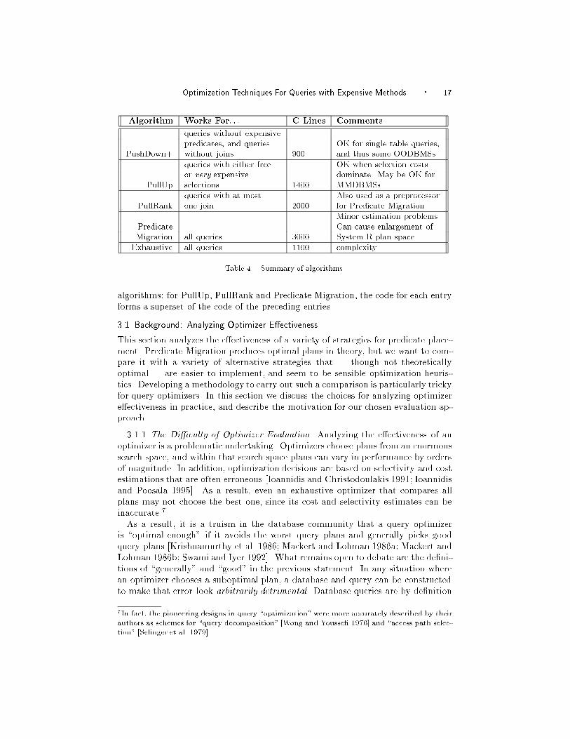
Table 4 provides a quick reference to the algorithms, their applicability and lim-
itations. When appropriate, the `C Lines' �eld gives a rough estimate of the total
number of lines of C code (with comments) needed in Illustra's System R-style
optimizer to support each algorithm. Note that much of the code is shared across
6Of course one may also choose to save particular subtrees for other reasons, such as \interesting
orders" [Selinger et al. 1979].
Optimization Techniques For Queries with Expensive Methods � 17
Algorithm Works For: : : C Lines Comments
queries without expensive
predicates, and queries OK for single table queries,
PushDown+ without joins 900 and thus some OODBMSs.
queries with either free OK when selection costs
or very expensive dominate. May be OK for
PullUp selections 1400 MMDBMSs.
queries with at most Also used as a preprocessor
PullRank one join 2000 for Predicate Migration.
Minor estimation problems.
Predicate Can cause enlargement of
Migration all queries 3000 System R plan space.
Exhaustive all queries 1100 complexity.
Table 4. Summary of algorithms.
algorithms: for PullUp, PullRank and Predicate Migration, the code for each entry
forms a superset of the code of the preceding entries.
3.1 Background: Analyzing Optimizer E�ectiveness
This section analyzes the e�ectiveness of a variety of strategies for predicate place-
ment. Predicate Migration produces optimal plans in theory, but we want to com-
pare it with a variety of alternative strategies that | though not theoretically
optimal | are easier to implement, and seem to be sensible optimization heuris-
tics. Developing a methodology to carry out such a comparison is particularly tricky
for query optimizers. In this section we discuss the choices for analyzing optimizer
e�ectiveness in practice, and describe the motivation for our chosen evaluation ap-
proach.
3.1.1 The Di�culty of Optimizer Evaluation. Analyzing the e�ectiveness of an
optimizer is a problematic undertaking. Optimizers choose plans from an enormous
search space, and within that search space plans can vary in performance by orders
of magnitude. In addition, optimization decisions are based on selectivity and cost
estimations that are often erroneous [Ioannidis and Christodoulakis 1991; Ioannidis
and Poosala 1995]. As a result, even an exhaustive optimizer that compares all
plans may not choose the best one, since its cost and selectivity estimates can be
inaccurate.7
As a result, it is a truism in the database community that a query optimizer
is \optimal enough" if it avoids the worst query plans and generally picks good
query plans [Krishnamurthy et al. 1986; Mackert and Lohman 1986a; Mackert and
Lohman 1986b; Swami and Iyer 1992]. What remains open to debate are the de�ni-
tions of \generally" and \good" in the previous statement. In any situation where
an optimizer chooses a suboptimal plan, a database and query can be constructed
to make that error look arbitrarily detrimental. Database queries are by de�nition
7In fact, the pioneering designs in query \optimization" were more accurately described by their
authors as schemes for \query decomposition" [Wong and Yousse� 1976] and \access path selec-
tion" [Selinger et al. 1979].
18 � J.M. Hellerstein
ad hoc, which leaves us with a signi�cant problem: how does one intelligently an-
alyze the practical e�cacy of an inherently rough technique over an in�nite space
of inputs?
Three approaches to this problem have traditionally been taken in the literature.
|Micro-Benchmarks: Basic query operators can be executed, and an optimizer's
cost and selectivity modeling can be compared to actual performance. This is the
technique used to study the R* distributed DBMS [Mackert and Lohman 1986a;
Mackert and Lohman 1986b], and it is very e�ective for isolating inaccuracies in
an optimizer's cost model.
|Randomized Macro-Benchmarks: Random data sets and queries can be
generated, and various optimization techniques used to generate competing plans.
This approach has been used in many studies (e.g., [Swami and Gupta 1988],
[Ioannidis and Kang 1990], [Hong and Stonebraker 1993], etc.) to give a rough
sense of average-case optimizer e�ectiveness, over a large space of workloads.
|StandardMacro-Benchmarks: An in uential person or committee can de�ne
a standard representative workload (data and queries), and di�erent strategies
can be compared on this workload. Examples of such benchmarks include the
Wisconsin benchmark [Bitton et al. 1983], AS3AP [Turby�ll et al. 1989], and
TPC-D [Raab 1995]. Such domain-speci�c benchmarks [Gray 1991] are often
based on models of real-world workloads. Standard benchmarks typically expose
whether or not a system implements solutions to important details exposed by
the benchmark, e.g. use of indices and reordering of joins in the Wisconsin bench-
mark, or intelligent handling of complex subqueries in TPC-D. If an optimizer
chooses a particular execution strategy then it does well, otherwise it does quite
poorly. The evaluation of the optimizer in these benchmarks is binary, in the
sense that typically the relative performance of the good and bad strategies is
not interesting; what is important is that the optimizer choose the \correct ac-
cess plan" [Turby�ll et al. 1989]. It is worth noting that these binary benchmarks
have proven extremely in uential, both in the commercial arena and in justifying
new optimizer research (especially in the case of TPC-D).
An alternative to benchmarking is to run queries that expose the logic that makes
one optimization strategy work where another fails. This binary outlook is quite
similar to the way in which the Wisconsin and TPC-D benchmarks re ect optimizer
e�ectiveness, but is di�erent in the sense that there is no claim that the workload
re ects any typical real-world scenario. Rather than being a \performance study"
in any practical sense, this is a form of empirical algorithm analysis, providing
insight into the algorithms rather than a quantitative comparison. The conclusion
of such an analysis is not to identify which optimization strategy should be used in
practice, but rather to highlight when and why each of the various schemes succeeds
and fails. This avoids the issue of identifying a \typical" workload, and hopefully
presents enough information to predict the behavior of each strategy for any such
workload.
Extensible database management systems are only now being deployed in com-
ercial settings, so there is little consensus on the de�nition of a real-world workload
containing expensive methods. As a result we decided not to de�ne a macro-
benchmark for expensive methods. We could have devised micro-benchmarks to
Optimization Techniques For Queries with Expensive Methods � 19
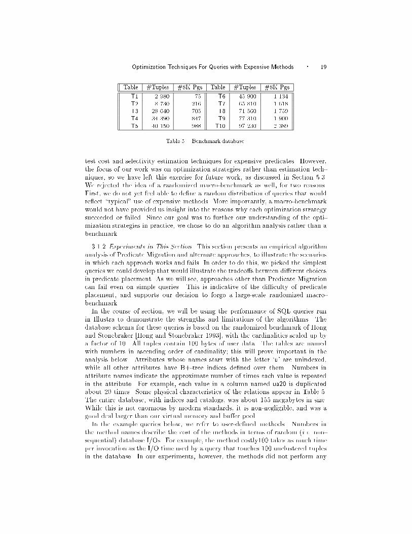
Table #Tuples #8K Pgs Table #Tuples #8K Pgs
T1 2 980 75 T6 45 900 1 134
T2 8 730 216 T7 65 810 1 618
T3 28 640 705 T8 71 560 1 759
T4 34 390 847 T9 77 310 1 900
T5 40 150 988 T10 97 230 2 389
Table 5. Benchmark database.
test cost and selectivity estimation techniques for expensive predicates. However,
the focus of our work was on optimization strategies rather than estimation tech-
niques, so we have left this exercise for future work, as discussed in Section 5.3.
We rejected the idea of a randomized macro-benchmark as well, for two reasons.
First, we do not yet feel able to de�ne a random distribution of queries that would
re ect \typical" use of expensive methods. More importantly, a macro-benchmark
would not have provided us insight into the reasons why each optimization strategy
succeeded or failed. Since our goal was to further our understanding of the opti-
mization strategies in practice, we chose to do an algorithm analysis rather than a
benchmark.
3.1.2 Experiments in This Section. This section presents an empirical algorithm
analysis of Predicate Migration and alternate approaches, to illustrate the scenarios
in which each approach works and fails. In order to do this, we picked the simplest
queries we could develop that would illustrate the tradeo�s between di�erent choices
in predicate placement. As we will see, approaches other than Predicate Migration
can fail even on simple queries. This is indicative of the di�culty of predicate
placement, and supports our decision to forgo a large-scale randomized macro-
benchmark.
In the course of section, we will be using the performance of SQL queries run
in Illustra to demonstrate the strengths and limitations of the algorithms. The
database schema for these queries is based on the randomized benchmark of Hong
and Stonebraker [Hong and Stonebraker 1993], with the cardinalities scaled up by
a factor of 10. All tuples contain 100 bytes of user data. The tables are named
with numbers in ascending order of cardinality; this will prove important in the
analysis below. Attributes whose names start with the letter `u' are unindexed,
while all other attributes have B+-tree indices de�ned over them. Numbers in
attribute names indicate the approximate number of times each value is repeated
in the attribute. For example, each value in a column named ua20 is duplicated
about 20 times. Some physical characteristics of the relations appear in Table 5.
The entire database, with indices and catalogs, was about 155 megabytes in size.
While this is not enormous by modern standards, it is non-negligible, and was a
good deal larger than our virtual memory and bu�er pool.
In the example queries below, we refer to user-de�ned methods. Numbers in
the method names describe the cost of the methods in terms of random (i.e. non-
sequential) database I/Os. For example, the method costly100 takes as much time
per invocation as the I/O time used by a query that touches 100 unclustered tuples
in the database. In our experiments, however, the methods did not perform any
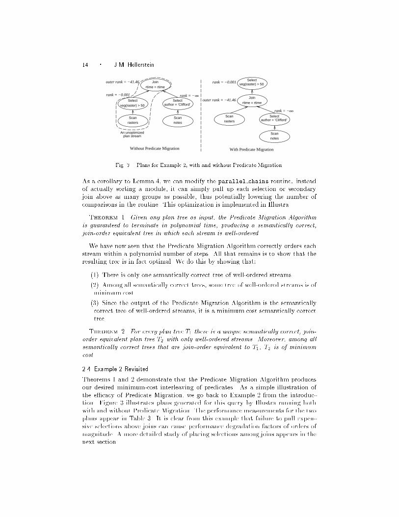
20 � J.M. Hellerstein
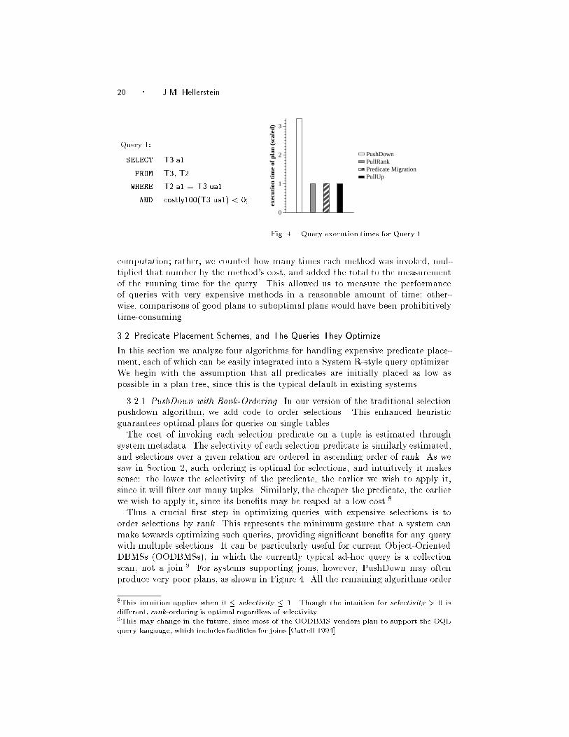
Query 1:
SELECT T3.a1
FROM T3, T2
WHERE T2.a1 = T3.ua1
AND costly100(T3.ua1) < 0;
0
1
2
3
exec
utio
n ti
me
of p
lan
(sca
led)
PushDownPullRankPredicate MigrationPullUp
Fig. 4. Query execution times for Query 1.
computation; rather, we counted how many times each method was invoked, mul-
tiplied that number by the method's cost, and added the total to the measurement
of the running time for the query. This allowed us to measure the performance
of queries with very expensive methods in a reasonable amount of time; other-
wise, comparisons of good plans to suboptimal plans would have been prohibitively
time-consuming.
3.2 Predicate Placement Schemes, and The Queries They Optimize
In this section we analyze four algorithms for handling expensive predicate place-
ment, each of which can be easily integrated into a System R-style query optimizer.
We begin with the assumption that all predicates are initially placed as low as
possible in a plan tree, since this is the typical default in existing systems.
3.2.1 PushDown with Rank-Ordering. In our version of the traditional selection
pushdown algorithm, we add code to order selections. This enhanced heuristic
guarantees optimal plans for queries on single tables.
The cost of invoking each selection predicate on a tuple is estimated through
system metadata. The selectivity of each selection predicate is similarly estimated,
and selections over a given relation are ordered in ascending order of rank. As we
saw in Section 2, such ordering is optimal for selections, and intuitively it makes
sense: the lower the selectivity of the predicate, the earlier we wish to apply it,
since it will �lter out many tuples. Similarly, the cheaper the predicate, the earlier
we wish to apply it, since its bene�ts may be reaped at a low cost.8
Thus a crucial �rst step in optimizing queries with expensive selections is to
order selections by rank. This represents the minimum gesture that a system can
make towards optimizing such queries, providing signi�cant bene�ts for any query
with multiple selections. It can be particularly useful for current Object-Oriented
DBMSs (OODBMSs), in which the currently typical ad-hoc query is a collection
scan, not a join.9 For systems supporting joins, however, PushDown may often
produce very poor plans, as shown in Figure 4. All the remaining algorithms order
8This intuition applies when 0 � selectivity � 1. Though the intuition for selectivity > 0 is
di�erent, rank-ordering is optimal regardless of selectivity.9This may change in the future, since most of the OODBMS vendors plan to support the OQL
query language, which includes facilities for joins [Cattell 1994].
Optimization Techniques For Queries with Expensive Methods � 21
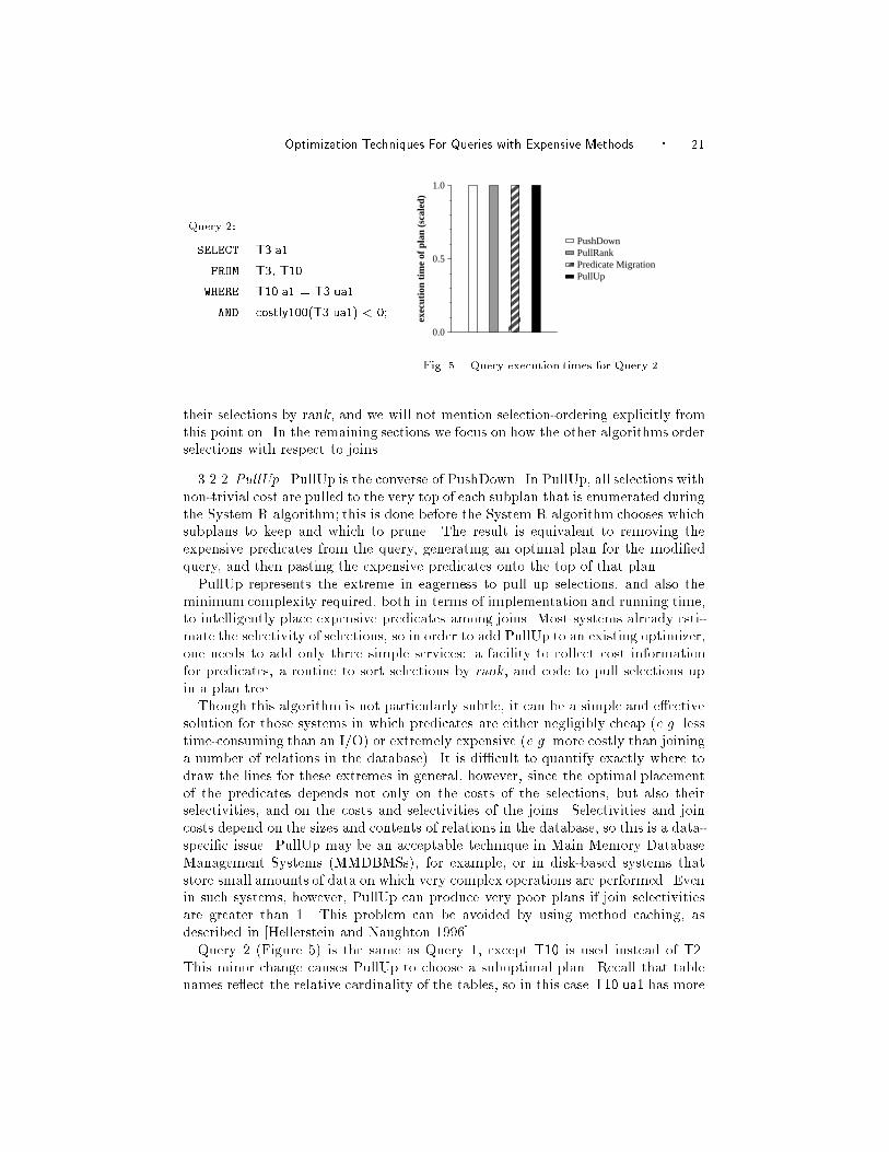
Query 2:
SELECT T3.a1
FROM T3, T10
WHERE T10.a1 = T3.ua1
AND costly100(T3.ua1) < 0;
0.0
0.5
1.0
exec
utio
n ti
me
of p
lan
(sca
led)
PushDownPullRankPredicate MigrationPullUp
Fig. 5. Query execution times for Query 2.
their selections by rank, and we will not mention selection-ordering explicitly from
this point on. In the remaining sections we focus on how the other algorithms order
selections with respect to joins.
3.2.2 PullUp. PullUp is the converse of PushDown. In PullUp, all selections with
non-trivial cost are pulled to the very top of each subplan that is enumerated during
the System R algorithm; this is done before the System R algorithm chooses which
subplans to keep and which to prune. The result is equivalent to removing the
expensive predicates from the query, generating an optimal plan for the modi�ed
query, and then pasting the expensive predicates onto the top of that plan.
PullUp represents the extreme in eagerness to pull up selections, and also the
minimum complexity required, both in terms of implementation and running time,
to intelligently place expensive predicates among joins. Most systems already esti-
mate the selectivity of selections, so in order to add PullUp to an existing optimizer,
one needs to add only three simple services: a facility to collect cost information
for predicates, a routine to sort selections by rank, and code to pull selections up
in a plan tree.
Though this algorithm is not particularly subtle, it can be a simple and e�ective
solution for those systems in which predicates are either negligibly cheap (e.g. less
time-consuming than an I/O) or extremely expensive (e.g. more costly than joining
a number of relations in the database). It is di�cult to quantify exactly where to
draw the lines for these extremes in general, however, since the optimal placement
of the predicates depends not only on the costs of the selections, but also their
selectivities, and on the costs and selectivities of the joins. Selectivities and join
costs depend on the sizes and contents of relations in the database, so this is a data-
speci�c issue. PullUp may be an acceptable technique in Main Memory Database
Management Systems (MMDBMSs), for example, or in disk-based systems that
store small amounts of data on which very complex operations are performed. Even
in such systems, however, PullUp can produce very poor plans if join selectivities
are greater than 1. This problem can be avoided by using method caching, as
described in [Hellerstein and Naughton 1996].
Query 2 (Figure 5) is the same as Query 1, except T10 is used instead of T2.This minor change causes PullUp to choose a suboptimal plan. Recall that table
names re ect the relative cardinality of the tables, so in this case T10.ua1 has more
22 � J.M. Hellerstein
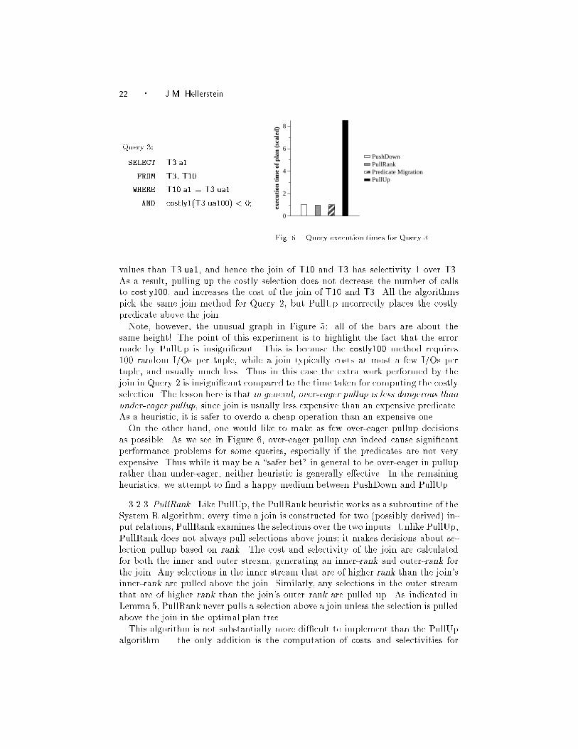
Query 3:
SELECT T3.a1
FROM T3, T10
WHERE T10.a1 = T3.ua1
AND costly1(T3.ua100) < 0;
0
2
4
6
8
exec
utio
n ti
me
of p
lan
(sca
led)
PushDownPullRankPredicate MigrationPullUp
Fig. 6. Query execution times for Query 3.
values than T3.ua1, and hence the join of T10 and T3 has selectivity 1 over T3.As a result, pulling up the costly selection does not decrease the number of calls
to costly100, and increases the cost of the join of T10 and T3. All the algorithms
pick the same join method for Query 2, but PullUp incorrectly places the costly
predicate above the join.
Note, however, the unusual graph in Figure 5: all of the bars are about the
same height! The point of this experiment is to highlight the fact that the error
made by PullUp is insigni�cant. This is because the costly100 method requires
100 random I/Os per tuple, while a join typically costs at most a few I/Os per
tuple, and usually much less. Thus in this case the extra work performed by the
join in Query 2 is insigni�cant compared to the time taken for computing the costly
selection. The lesson here is that in general, over-eager pullup is less dangerous than
under-eager pullup, since join is usually less expensive than an expensive predicate.
As a heuristic, it is safer to overdo a cheap operation than an expensive one.
On the other hand, one would like to make as few over-eager pullup decisions
as possible. As we see in Figure 6, over-eager pullup can indeed cause signi�cant
performance problems for some queries, especially if the predicates are not very
expensive. Thus while it may be a \safer bet" in general to be over-eager in pullup
rather than under-eager, neither heuristic is generally e�ective. In the remaining
heuristics, we attempt to �nd a happy medium between PushDown and PullUp.
3.2.3 PullRank. Like PullUp, the PullRank heuristic works as a subroutine of the
System R algorithm: every time a join is constructed for two (possibly derived) in-
put relations, PullRank examines the selections over the two inputs. Unlike PullUp,
PullRank does not always pull selections above joins; it makes decisions about se-
lection pullup based on rank. The cost and selectivity of the join are calculated
for both the inner and outer stream, generating an inner-rank and outer-rank for
the join. Any selections in the inner stream that are of higher rank than the join's
inner-rank are pulled above the join. Similarly, any selections in the outer stream
that are of higher rank than the join's outer rank are pulled up. As indicated in
Lemma 5, PullRank never pulls a selection above a join unless the selection is pulled
above the join in the optimal plan tree.
This algorithm is not substantially more di�cult to implement than the PullUp
algorithm | the only addition is the computation of costs and selectivities for
Optimization Techniques For Queries with Expensive Methods � 23
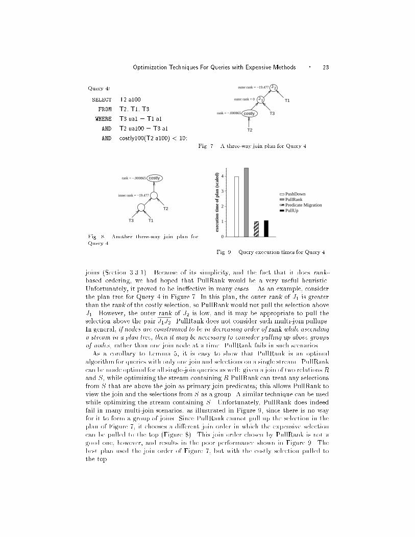
Query 4:
SELECT T2.a100
FROM T2, T1, T3
WHERE T3.ua1 = T1.a1
AND T2.ua100 = T3.a1
AND costly100(T2.a100) < 10;
J 1
J 2
outer rank = 0
costlyrank = −.000865
outer rank = −19.477
T2
T3
T1
Fig. 7. A three-way join plan for Query 4.
costlyrank = −.000865
inner rank = −19.477
T2
T1T3
Fig. 8. Another three-way join plan for
Query 4.
0
1
2
3
4
exec
utio
n ti
me
of p
lan
(sca
led)
PushDownPullRankPredicate MigrationPullUp
Fig. 9. Query execution times for Query 4.
joins (Section 3.3.1). Because of its simplicity, and the fact that it does rank-
based ordering, we had hoped that PullRank would be a very useful heuristic.
Unfortunately, it proved to be ine�ective in many cases. As an example, consider
the plan tree for Query 4 in Figure 7. In this plan, the outer rank of J1 is greater
than the rank of the costly selection, so PullRank would not pull the selection above
J1. However, the outer rank of J2 is low, and it may be appropriate to pull the
selection above the pair J1J2. PullRank does not consider such multi-join pullups.
In general, if nodes are constrained to be in decreasing order of rank while ascending
a stream in a plan tree, then it may be necessary to consider pulling up above groups
of nodes, rather than one join node at a time. PullRank fails in such scenarios.
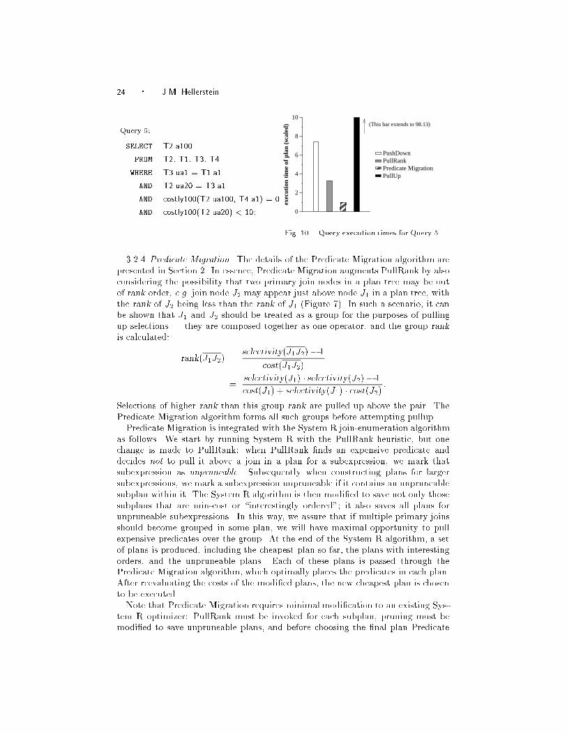
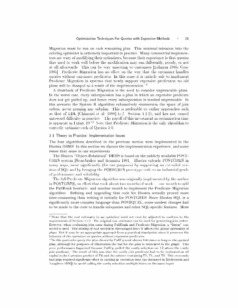
As a corollary to Lemma 5, it is easy to show that PullRank is an optimal
algorithm for queries with only one join and selections on a single stream. PullRank
can be made optimal for all single-join queries as well: given a join of two relations R
and S, while optimizing the stream containing R PullRank can treat any selections
from S that are above the join as primary join predicates; this allows PullRank to
view the join and the selections from S as a group. A similar technique can be used
while optimizing the stream containing S. Unfortunately, PullRank does indeed
fail in many multi-join scenarios, as illustrated in Figure 9, since there is no way
for it to form a group of joins. Since PullRank cannot pull up the selection in the
plan of Figure 7, it chooses a di�erent join order in which the expensive selection
can be pulled to the top (Figure 8). This join order chosen by PullRank is not a
good one, however, and results in the poor performance shown in Figure 9. The
best plan used the join order of Figure 7, but with the costly selection pulled to
the top.
24 � J.M. Hellerstein
Query 5:
SELECT T2.a100
FROM T2, T1, T3, T4
WHERE T3.ua1 = T1.a1
AND T2.ua20 = T3.a1
AND costly100(T2.ua100, T4.a1) = 0
AND costly100(T2.ua20) < 10; 0
2
4
6
8
10
exec
utio
n ti
me
of p
lan
(sca
led)
PushDownPullRankPredicate MigrationPullUp
(This bar extends to 98.13)
Fig. 10. Query execution times for Query 5.
3.2.4 Predicate Migration. The details of the Predicate Migration algorithm are
presented in Section 2. In essence, Predicate Migration augments PullRank by also
considering the possibility that two primary join nodes in a plan tree may be out
of rank order, e.g. join node J2 may appear just above node J1 in a plan tree, with
the rank of J2 being less than the rank of J1 (Figure 7). In such a scenario, it can
be shown that J1 and J2 should be treated as a group for the purposes of pulling
up selections | they are composed together as one operator, and the group rank
is calculated:
rank(J1J2) =selectivity(J1J2) � 1
cost(J1J2)
=selectivity(J1) � selectivity(J2) � 1
cost(J1) + selectivity(J1) � cost(J2):
Selections of higher rank than this group rank are pulled up above the pair. The
Predicate Migration algorithm forms all such groups before attempting pullup.
Predicate Migration is integrated with the System R join-enumeration algorithm
as follows. We start by running System R with the PullRank heuristic, but one
change is made to PullRank: when PullRank �nds an expensive predicate and
decides not to pull it above a join in a plan for a subexpression, we mark that
subexpression as unpruneable. Subsequently when constructing plans for larger
subexpressions, we mark a subexpression unpruneable if it contains an unpruneable
subplan within it. The System R algorithm is then modi�ed to save not only those
subplans that are min-cost or \interestingly ordered"; it also saves all plans for
unpruneable subexpressions. In this way, we assure that if multiple primary joins
should become grouped in some plan, we will have maximal opportunity to pull
expensive predicates over the group. At the end of the System R algorithm, a set
of plans is produced, including the cheapest plan so far, the plans with interesting
orders, and the unpruneable plans. Each of these plans is passed through the
Predicate Migration algorithm, which optimally places the predicates in each plan.
After reevaluating the costs of the modi�ed plans, the new cheapest plan is chosen
to be executed.
Note that Predicate Migration requires minimal modi�cation to an existing Sys-
tem R optimizer: PullRank must be invoked for each subplan, pruning must be
modi�ed to save unpruneable plans, and before choosing the �nal plan Predicate
Optimization Techniques For Queries with Expensive Methods � 25
Migration must be run on each remaining plan. This minimal intrusion into the
existing optimizer is extremely important in practice. Many commercial implemen-
tors are wary of modifying their optimizers, because their experience is that queries
that used to work well before the modi�cation may run di�erently, poorly, or not
at all afterwards. This can be very upsetting to customers [Lohman 1995; Gray
1995]. Predicate Migration has no e�ect on the way that the optimizer handles
queries without expensive predicates. In this sense it is entirely safe to implement
Predicate Migration in systems that newly support expensive predicates; no old
plans will be changed as a result of the implementation.10
A drawback of Predicate Migration is the need to consider unpruneable plans.
In the worst case, every subexpression has a plan in which an expensive predicate
does not get pulled up, and hence every subexpression is marked unpruneable. In
this scenario the System R algorithm exhaustively enumerates the space of join
orders, never pruning any subplan. This is preferable to earlier approaches such
as that of LDL [Chimenti et al. 1989] (c.f. Section 4.1.2), and has not caused
untoward di�culty in practice. The payo� of this investment in optimization time
is apparent in Figure 10.11 Note that Predicate Migration is the only algorithm to
correctly optimize each of Queries 1-5.
3.3 Theory to Practice: Implementation Issues
The four algorithms described in the previous section were implemented in the
Illustra DBMS. In this section we discuss the implementation experience, and some
issues that arose in our experiments.
The Illustra \Object-Relational" DBMS is based on the publicly available POST-
GRES system [Stonebraker and Kemnitz 1991]. Illustra extends POSTGRES in
many ways, most signi�cantly (for our purposes) by supporting an extended ver-
sion of SQL and by bringing the POSTGRES prototype code to an industrial grade
of performance and reliability.
The full Predicate Migration algorithmwas originally implemented by the author
in POSTGRES, an e�ort that took about two months of work | one month to add
the PullRank heuristic, and another month to implement the Predicate Migration
algorithm. Re�ning and upgrading that code for Illustra actually proved more
time-consuming than writing it initially for POSTGRES. Since Illustra SQL is a
signi�cantly more complex language than POSTQUEL, some modest changes had
to be made to the code to handle subqueries and other SQL-speci�c features. More
10Note that the cost estimates in an optimizer need not even be adjusted to conform to the
requirements of Section 3.3.1. The original cost estimates can be used for generating join orders.
However, when evaluating join costs during PullRank and Predicate Migration, a \linear" cost
model is used. This mixing of cost models is discouraged since it a�ects the global optimality of
plans. But it may be an appropriate approach from a practical standpoint, since it preserves the
behavior of the optimizer on queries without expensive predicates.11In this particular query the plan chosen by PullUp took almost 100 times as long as the optimal
plan, although for purposes of illustration the bar for the plan is truncated in the graph. This
poor performance happened because PullUp pulled the costly selection on T2 above the costly
join predicate. The result of this was that the costly join predicate had to be evaluated on all
tuples in the Cartesian product of T4 and the subtree containingT2, T1, and T3. This extremely
bad plan required signi�cant e�ort in caching at execution time (as discussed in [Hellerstein and
Naughton 1996]) to avoid calling the costly selection multiple times on the same input.
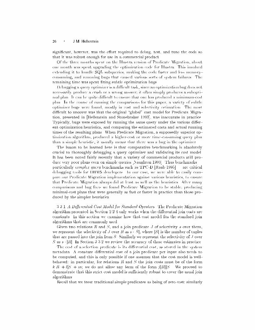
26 � J.M. Hellerstein
signi�cant, however, was the e�ort required to debug, test, and tune the code so
that it was robust enough for use in a commercial product.
Of the three months spent on the Illustra version of Predicate Migration, about
one month was spent upgrading the optimization code for Illustra. This involved
extending it to handle SQL subqueries, making the code faster and less memory-
consuming, and removing bugs that caused various sorts of system failures. The
remaining time was spent �xing subtle optimization bugs.
Debugging a query optimizer is a di�cult task, since an optimizationbug does not
necessarily produce a crash or a wrong answer; it often simply produces a subopti-
mal plan. It can be quite di�cult to ensure that one has produced a minimum-cost
plan. In the course of running the comparisons for this paper, a variety of subtle
optimizer bugs were found, mostly in cost and selectivity estimation. The most
di�cult to uncover was that the original \global" cost model for Predicate Migra-
tion, presented in [Hellerstein and Stonebraker 1993], was inaccurate in practice.
Typically, bugs were exposed by running the same query under the various di�er-
ent optimization heuristics, and comparing the estimated costs and actual running
times of the resulting plans. When Predicate Migration, a supposedly superior op-
timization algorithm, produced a higher-cost or more time-consuming query plan
than a simple heuristic, it usually meant that there was a bug in the optimizer.
The lesson to be learned here is that comparative benchmarking is absolutely
crucial to thoroughly debugging a query optimizer and validating its cost model.
It has been noted fairly recently that a variety of commercial products still pro-
duce very poor plans even on simple queries [Naughton 1993]. Thus benchmarks |
particularly complex query benchmarks such as TPC-D [Raab 1995] | are critical
debugging tools for DBMS developers. In our case, we were able to easily com-
pare our Predicate Migration implementation against various heuristics, to ensure
that Predicate Migration always did at least as well as the heuristics. After many
comparisons and bug �xes we found Predicate Migration to be stable, producing
minimal-cost plans that were generally as fast or faster in practice than those pro-
duced by the simpler heuristics.
3.3.1 A Di�erential Cost Model for Standard Oprators. The Predicate Migration
algorithm presented in Section 2.2.4 only works when the di�erential join costs are
constants. In this section we examine how that cost model �ts the standard join
algorithms that are commonly used.
Given two relations R and S, and a join predicate J of selectivity s over them,
we represent the selectivity of J over R as s � jSj, where jSj is the number of tuples
that are passed into the join from S. Similarly we represent the selectivity of J over
S as s � jRj. In Section 3.3.2 we review the accuracy of these estimates in practice.
The cost of a selection predicate is its di�erential cost, as stored in the system
metadata. A constant di�erential cost of a join predicate per input also needs to
be computed, and this is only possible if one assumes that the cost model is well-
behaved: in particular, for relations R and S the join costs must be of the form
kjRj + ljSj + m; we do not allow any term of the form jjRjjSj. We proceed to
demonstrate that this strict cost model is su�ciently robust to cover the usual join
algorithms.
Recall that we treat traditional simple predicates as being of zero cost; similarly
Optimization Techniques For Queries with Expensive Methods � 27
here we ignore the CPU costs associated with joins. In terms of I/O, the costs
of merge and hash joins given by Shapiro, et al. [Shapiro 1986] �t our criterion.12
For nested-loop join with an indexed inner relation, the cost per tuple of the outer
relation is the cost of probing the index (typically 3 I/Os or less), while the cost
per tuple of the inner relation is essentially zero | since we never scan tuples of
the inner relation that do not qualify for the join, they are �ltered with zero cost.
So nested-loop join with an indexed inner relation �ts our criterion as well.
The trickiest issue is that of nested-loop join without an index. In this case, the
cost is jjRj[S]+kjRj+ ljSj+m, where [S] is the number of blocks scanned from the
inner relation S. Note that the number of blocks scanned from the inner relation
is a constant irrespective of expensive selections on the inner relation. That is, in a
nested-loop join, for each tuple of the outer relation one must scan every disk block
of the inner relation, regardless of whether expensive selections are pulled up from
the inner relation or not. So nested-loop join does indeed �t our cost model: [S]
is a constant regardless of where expensive predicates are placed, and the equation
above can be written as (j[S] + k)jRj + ljSj + m.13 Therefore we can accurately
model the di�erential costs of all the typical join methods per tuple of an input.
These \linear" cost models have been evaluated experimentally for nested-loop
and merge joins, and were found to be relatively accurate estimates of the perfor-
mance of a variety of commercial systems [Du et al. 1992].
3.3.2 In uence of Performance Results on Estimates. The results of our perfor-
mance experiments in uenced the way that we estimate selectivities in Illustra.
In the previus section, we estimated the selectivity of a join over table S as s � jRj.
This was a rough estimate, however, since jRj is not well de�ned | it depends on
the selections that are placed on R. Thus jRj could range from the cardinality of
R with no selections, to the minimal output of R after all eligible selections are
applied. In Illustra, we calculate jRj on the y as needed, based on the number
of selections over R at the time that we need to compute the selectivity of the
join. Since some predicates over R may later be pulled up, this potentially under-
estimates the selectivity of the join for S. Such an under-estimate results in an
under-estimate of the rank of the join for S, possibly resulting in over-eager pullup
of selections on S. This rough selectivity estimation was chosen as a result of our
performance observations: it was decided that estimates resulting in somewhat over-
eager pullup are preferable to estimates resulting in under-eager pullup. In part,
this heuristic is based on the existence of method caching in Illustra, as described
in [Hellerstein and Naughton 1996] | as long as methods are cached, pulling a
selection above a join incorrectly cannot increase the number of times the selection
method is actually computed, it can only increase the number of duplicate input
values to the selection.
The potential for over-eager pullup in Predicate Migration is similar, though
12Actually, we ignore thepS savings available in merge join due to bu�ering. We thus slightly
over-estimate the costs of merge join for the purposes of predicate placement.13This assumes that plan trees are left-deep, which is true for many systems including Illustra.
Even for bushy trees this is not a signi�cant limitation: one would be unlikely to have nested-loop
join with a bushy inner, since one might as well sort or hash the inner relation while materializing
it.
28 � J.M. Hellerstein
not as agrant, as the over-eager pullup in the earlier LDL approach [Chimenti
et al. 1989], described in Section 4.1.2. Observe that if the Predicate Migration
approach pulls up from inner inputs �rst, then ranks of joins for inner inputs may
be underestimated, but ranks of joins for outer inputs are accurate, since pullup
from the inner input has already been completed. This will produce over-eager
pullup from inner tables, and accurate pullup from outer tables, which also occurs
in LDL. This is the approach taken in Illustra, but unlike LDL, Illustra only exhibits
this over-eagerness in a very constrained situation:
(1) when there are expensive selections on both inputs to a join, and
(2) some of the expensive selections on the outer input should be pulled up, and
(3) some of the expensive selections on the inner input should not be pulled up,
and
(4) treating the inner input before the outer results in selectivity estimations
that cause over-eager pullup of some of those selections from the inner input.
By contrast, the LDL approach pulls up expensive predicates from inner inputs in
all circumstances.
4. RELATED WORK
4.1 Optimization and Expensive Methods
4.1.1 Predicate Migration. Stonebraker raised the issue of expensive predicate
optimization in the context of the POSTGRES multi-level store [Stonebraker 1991].
The questions posed by Stonebraker are directly addressed in this paper.
Predicate Migration was �rst presented in 1992 [Hellerstein and Stonebraker
1993]. While the Predicate Migration Algorithm presented there was identical
to the one described in Section 2.2.4 of this paper, the early paper included a
\global" cost model which was inaccurate in modeling query cost; in particular, it
modeled the selectivity of a join as being identical with respect to both inputs. A
later paper [Hellerstein 1994] presented the corrected cost model described here in
Section 3.3.1 This paper extends our previous work with a thorough and correct
discussion of cost model issues, proofs of optimality and pseudocode for Predicate
Migration, and new experimental measurements using a later version of Illustra
enhanced with method caching techniques.
4.1.2 The LDL Approach. The �rst approach for optimizing queries with expen-
sive predicates was pioneered in the LDL logic database system [Chimenti et al.
1989], and was proposed for extensible relational systems by Yajima, et al. [Yajima
et al. 1991]. We refer to this as the LDL approach. To illustrate this approach,
consider the following example query:
SELECT *
FROM R, S
WHERE R.c1 = S.c1
AND p(R.c2)
AND q(S.c2);
In the query, p and q are expensive user-de�ned Boolean methods.
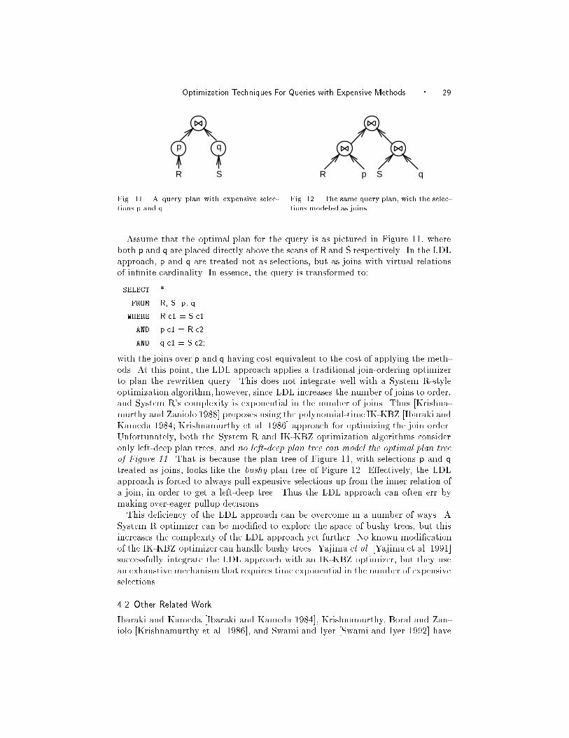
Optimization Techniques For Queries with Expensive Methods � 29
p q
R S
Fig. 11. A query plan with expensive selec-
tions p and q.
p qR S
Fig. 12. The same query plan, with the selec-
tions modeled as joins.
Assume that the optimal plan for the query is as pictured in Figure 11, where
both p and q are placed directly above the scans of R and S respectively. In the LDLapproach, p and q are treated not as selections, but as joins with virtual relations
of in�nite cardinality. In essence, the query is transformed to:
SELECT *
FROM R, S, p, q
WHERE R.c1 = S.c1
AND p.c1 = R.c2
AND q.c1 = S.c2;
with the joins over p and q having cost equivalent to the cost of applying the meth-
ods. At this point, the LDL approach applies a traditional join-ordering optimizer
to plan the rewritten query. This does not integrate well with a System R-style
optimization algorithm, however, since LDL increases the number of joins to order,
and System R's complexity is exponential in the number of joins. Thus [Krishna-
murthy and Zaniolo 1988] proposes using the polynomial-time IK-KBZ [Ibaraki and
Kameda 1984; Krishnamurthy et al. 1986] approach for optimizing the join order.
Unfortunately, both the System R and IK-KBZ optimization algorithms consider
only left-deep plan trees, and no left-deep plan tree can model the optimal plan tree
of Figure 11. That is because the plan tree of Figure 11, with selections p and qtreated as joins, looks like the bushy plan tree of Figure 12. E�ectively, the LDL
approach is forced to always pull expensive selections up from the inner relation of
a join, in order to get a left-deep tree. Thus the LDL approach can often err by
making over-eager pullup decisions.
This de�ciency of the LDL approach can be overcome in a number of ways. A
System R optimizer can be modi�ed to explore the space of bushy trees, but this
increases the complexity of the LDL approach yet further. No known modi�cation
of the IK-KBZ optimizer can handle bushy trees. Yajima et al. [Yajima et al. 1991]
successfully integrate the LDL approach with an IK-KBZ optimizer, but they use
an exhaustive mechanism that requires time exponential in the number of expensive
selections.
4.2 Other Related Work
Ibaraki and Kameda [Ibaraki and Kameda 1984], Krishnamurthy, Boral and Zan-
iolo [Krishnamurthy et al. 1986], and Swami and Iyer [Swami and Iyer 1992] have
30 � J.M. Hellerstein
developed and re�ned a query optimization scheme that is built on the the notion
of rank. However, their scheme uses rank to reorder joins rather than selections.
Their techniques do not consider the possibility of expensive selection predicates,
and only reorder nodes of a single path in a left-deep query plan tree. Furthermore,
their schemes are a proposal for a completely new method for query optimization,
not an extension that can be applied to the plans of any query optimizer.
The System R project faced the issue of expensive predicate placement early
on, since their SQL language had the notion of subqueries, which (especially when
correlated) are a form of expensive selection. At the time, however, the emphasis of
their optimization work was on �nding optimal join orders and methods, and there
was no published work on placing expensive predicates in a query plan. System R
and R* both had simple heuristics for placing an expensive subquery in a plan.
In both systems, subquery evaluation was postponed until simple predicates were
evaluated. In R*, the issue of balancing selectivity and cost was discussed, but
in the �nal implementation subqueries were ordered among themselves by a cost-
only metric: the more di�cult the subquery was to compute, the later it would
be applied. Neither system considered pulling up subquery predicates from their
lowest eligible position [Lohman and Haas 1993].
An orthogonal issue related to predicate placement is the problem of rewriting
predicates into more e�cient forms [Chaudhuri and Shim 1993; Chen et al. 1992].
In such semantic optimization work, the focus is on rewriting expensive predicates
in terms of other, cheaper predicates. Another semantic rewriting technique called
\Predicate Move-Around" [Levy et al. 1994] suggests rewriting SQL queries by
copying predicates and then moving the copies across query blocks. The authors
conjecture that this technique may be bene�cial for queries with expensive predi-
cates. A related idea occurs in Object-Oriented databases, which can have \path
expression" methods that follow references from tuples to other tuples. A typi-
cal technique for such methods is to rewrite them as joins, and then submit the
query for traditional join optimization.14 All of these ideas are similar to the query
rewrite facility of Starburst [Pirahesh et al. 1992], in that they are heuristics for
rewriting a declarative query, rather than cost-based optimizations for converting a
declarative query into an execution plan. It is important to note that these issues
are indeed orthogonal to our problems of predicate placement | once queries have
been rewritten into cheaper forms, they still need to have their predicates optimally
placed into a query plan.
Kemper, Steinbrunn, et al. [Kemper et al. 1994; Steinbrunn et al. 1995] address
the problem of planning disjunctive queries with expensive predicates; their work
is not easily integrated with a traditional (conjunct-based) optimizer. Like most
System R-based optimizers, Illustra focuses on Boolean factors (conjuncts). Within
Boolean factors, the operands of OR are ordered by the metric cost/selectivity.
14A mixture of path expressions and (expensive) user-de�nedmethods is also possible, e.g. SELECT
* FROM emp WHERE emp.children.photo.haircolor() = 'red'. Such expressions can be rewrit-
ten in functional notation (e.g. SELECT * FROM emp WHERE haircolor(emp.children.photo) =
'red'), and are typically converted into joins (i.e., something like SELECT emp.* FROM emp,
kids WHERE emp.kid = kids.id and haircolor(kids.photo) = 'red', possibly with variations
to handle duplicate semantics). Note that an expensive method whose argument is a path expres-
sion becomes an expensive secondary join clause.
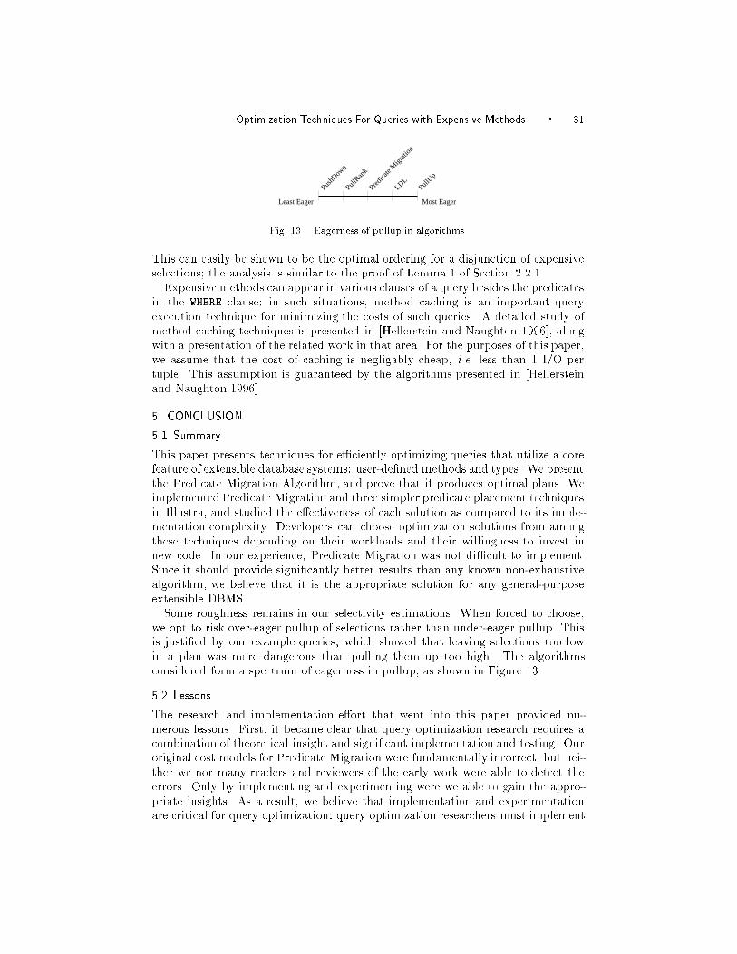
Optimization Techniques For Queries with Expensive Methods � 31
Predic
ate
Migr
ation
LDL
Most EagerLeast Eager
PullRan
k
PushD
own
PullUp
Fig. 13. Eagerness of pullup in algorithms.
This can easily be shown to be the optimal ordering for a disjunction of expensive
selections; the analysis is similar to the proof of Lemma 1 of Section 2.2.1.
Expensive methods can appear in various clauses of a query besides the predicates
in the WHERE clause; in such situations, method caching is an important query
execution technique for minimizing the costs of such queries. A detailed study of
method caching techniques is presented in [Hellerstein and Naughton 1996], along
with a presentation of the related work in that area. For the purposes of this paper,
we assume that the cost of caching is negligably cheap, i.e. less than 1 I/O per
tuple. This assumption is guaranteed by the algorithms presented in [Hellerstein
and Naughton 1996].
5. CONCLUSION
5.1 Summary
This paper presents techniques for e�ciently optimizing queries that utilize a core
feature of extensible database systems: user-de�ned methods and types. We present
the Predicate Migration Algorithm, and prove that it produces optimal plans. We
implemented Predicate Migration and three simpler predicate placement techniques
in Illustra, and studied the e�ectiveness of each solution as compared to its imple-
mentation complexity. Developers can choose optimization solutions from among
these techniques depending on their workloads and their willingness to invest in
new code. In our experience, Predicate Migration was not di�cult to implement.
Since it should provide signi�cantly better results than any known non-exhaustive
algorithm, we believe that it is the appropriate solution for any general-purpose
extensible DBMS.
Some roughness remains in our selectivity estimations. When forced to choose,
we opt to risk over-eager pullup of selections rather than under-eager pullup. This
is justi�ed by our example queries, which showed that leaving selections too low
in a plan was more dangerous than pulling them up too high. The algorithms
considered form a spectrum of eagerness in pullup, as shown in Figure 13.
5.2 Lessons
The research and implementation e�ort that went into this paper provided nu-
merous lessons. First, it became clear that query optimization research requires a
combination of theoretical insight and signi�cant implementation and testing. Our
original cost models for Predicate Migration were fundamentally incorrect, but nei-
ther we nor many readers and reviewers of the early work were able to detect the
errors. Only by implementing and experimenting were we able to gain the appro-
priate insights. As a result, we believe that implementation and experimentation
are critical for query optimization: query optimization researchers must implement
32 � J.M. Hellerstein
their ideas to demonstrate viability, and new complex query benchmarks are re-
quired to drive both researchers and industry into workable solutions to the many
remaining challenges in query optimization.
Implementing an e�ective predicate placement scheme proved to be a manage-
able task, and doing so exposed many over-simpli�cations that were present in the
original algorithms proposed. This highlights the complex issues that arise in im-
plementing query optimizers. Perhaps the most important lesson we learned in
implementing Predicate Migration in Illustra was that query optimizers require a
great deal of testing before they can be trusted. In practice this means that commer-
cial optimizers should be subjected to complex query benchmarks, and that query
optimization researchers should invest time in implementing and testing their ideas
in practice.
The limitations of the previously published algorithms for predicate placement
are suggestive. Both algorithms su�er from the same problem: the choice of which
predicates to pull up from one side of a join both depends on and in uences the
choice of which predicates to pull up from the other side of the join. This interde-
pendency of separate streams in a query tree suggests a fundamental intractability
in predicate placement, that may only be avoidable through the sorts of compro-
mises found in the existing literature.
5.3 Open Questions
This paper leaves a number of interesting questions open. It would be satisfying
to understand the rami�cations of weakening the assumptions of the Predicate
Migration cost model. Is our roughness in estimation required for a polynomial-
time predicate placement algorithm, or is there a way to weaken the assumptions
and still develop an e�cient algorithm?
This question can be cast in di�erent terms. If one combines the LDL ap-
proach for expensive methods [Chimenti et al. 1989] with the IK-KBZ rank-based
join optimizer [Ibaraki and Kameda 1984; Krishnamurthy et al. 1986], one gets a
polynomial-time optimization algorithm that handles expensive selections. How-
ever as we pointed out in Section 4.1.2 this technique fails because IK-KBZ does
not handle bushy join trees. So an isomorphic question to the one above is whether
the IK-KBZ join-ordering algorithm can be extended to handle bushy trees in poly-
nomial time. Recent work [Scheufele and Moerkotte 1997] shows that the answer
to this question is in general negative.
Although Predicate Migration does not signi�cantly a�ect the asymptotic cost of
exponential join-ordering query optimizers, it can noticeably increase the memory
utilization of the algorithms by preventing pruning. A useful extension of this work
would be a deeper investigation of techniques to allow even more pruning than
already available via PullRank during Predicate Migration.
Our work on predicate placement has concentrated on the traditional non-recursive
select-project-join query blocks that are handled by most cost-based optimizers. It
would be interesting to try and extend our work to more di�cult sorts of queries.
For example, how can Predicate Migration be applied to recursive queries and com-
mon subexpressions? When should predicates be transferred across query blocks?
When should they be duplicated across query blocks [Levy et al. 1994]? These
questions will require signi�cant e�ort to answer, since there are no generally ac-
Optimization Techniques For Queries with Expensive Methods � 33
cepted techniques for cost-based optimization in these scenarios, even for queries
without expensive predicates.
5.4 Suggestions for Implementation
Practitioners are often wary of adding large amounts of code to existing systems.
Fortunately, the work in this paper can be implemented incrementally, providing
increasing bene�ts as more pieces are added. We sketch a plausible upgrade path
for existing extensible systems:
(1) As a �rst step in optimization, selections should be ordered by rank (the
PushDown+ heuristic). Since typical optimizers already estimate selectivities,
this only requires estimating selection costs, and sorting selections.
(2) As a further enhancement, the PullUp heuristic can be implemented. This
requires code to pull selections above joins, which is a bit tricky since it requires
handling projections and column renumbering. Note that PullUp is not nec-
essarily more e�ective than PushDown for all queries, but is probably a safer
heuristic if methods are expected to be very expensive.
(3) The PullUp heuristic can be be modi�ed to do PullRank, by including code
to compute the di�erential costs for joins. Since PullRank can leave methods
too low in a plan, it is in some sense more dangerous than PullUp. On the
other hand, it can correctly optimize all two-table queries, which PullUp can
not guarantee. A decision between PullUp and PullRank is thus somewhat
di�cult { a compromise may be met by implementing both and choosing the
cheaper plan that comes out of the two. Since PullRank is a preprocessor for
a full implementation of Predicate Migration, it is a further step in the right
direction.
(4) Predicate Migration itself, while somewhat complex to understand, is ac-
tually not di�cult to implement. It requires implementation of the Predicate
Migration Algorithm, PullRank, and also code to mark subplans as unprune-
able.
(5) Finally, execution can be further improved by implementinga caching scheme
such as Hybrid Cache [Hellerstein and Naughton 1996] for expensive methods.
This requires some modi�cation of the cost model in the optimizer as well.
ACKNOWLEDGMENTS
Special thanks are due to Je� Naughton and Mike Stonebraker for their assistance
with this work. Thanks are also due to the sta� of Illustra InformationTechnologies,
particularly Paula Hawthorn, Wei Hong, Michael Ubell, Mike Olson, Je� Meredith,
and Kevin Brown. In addition, the following all provided useful input on this
paper: Surajit Chaudhuri, David DeWitt, James Frew, Jim Gray, Laura Haas,
Eugene Lawler, Guy Lohman, Raghu Ramakrishnan, and Praveen Seshadri.
REFERENCES
Bitton, D., DeWitt, D. J., and Turbyfill, C. 1983. Benchmarking database systems,
a systematic approach. In Proc. 9th International Conference on Very Large Data Bases
(Florence, Italy, Oct. 1983).
34 � J.M. Hellerstein
Boulos, J., Vi�emont, Y., and Ono, K. 1997. Analytical Models and Neural Networks for
Query Cost Evaluation. In Proc. 3rd International Workshop on Next Generation Infor-
mation Technology Systems (Neve Ilan, Israel, 1997).
Carey, M. J., DeWitt, D. J., Kant, C., and Naughton, J. F. 1994. A Status Report
on the OO7 OODBMS Benchmarking E�ort. In Proc. Conference on Object-Oriented Pro-
gramming Systems, Languages, and Applications (Portland, Oct. 1994), pp. 414{426.
Cattell, R. 1994. The Object Database Standard: ODMG-93 (Release 1.1). Morgan Kauf-
mann, San Mateo, CA.
Chaudhuri, S. and Shim, K. 1993. Query Optimization in the Presence of Foreign Func-
tions. In Proc. 19th International Conference on Very Large Data Bases (Dublin, Aug.
1993), pp. 526{541.
Chen, H., Yu, X., Yamaguchi, K., Kitagawa, H., Ohbo, N., and Fujiwara, Y. 1992.
Decomposition | An Approach for Optimizing Queries Including ADT Functions. Infor-
mation Processing Letters 43, 6, 327{333.
Chimenti, D., Gamboa, R., and Krishnamurthy, R. 1989. Towards an Open Architecture
for LDL. In Proc. 15th International Conference on Very Large Data Bases (Amsterdam,
Aug. 1989), pp. 195{203.
Dayal, U. 1987. Of Nests and Trees: A Uni�ed Approach to Processing Queries that Con-
tain Nested Subqueries, Aggregates, and Quanti�ers. In Proc. 13th International Confer-
ence on Very Large Data Bases (Brighton, Sept. 1987), pp. 197{208.
Du, W., Krishnamurthy, R., and Shan, M.-C. 1992. Query Optimization in Heteroge-
neous DBMS. In Proc. 18th International Conference on Very Large Data Bases (Vancou-
ver, Aug. 1992), pp. 277{291.
Faloutsos, C. and Kamel, I. 1994. Beyond Uniformity and Independence: Analysis of
R-trees Using the Concept of Fractal Dimension. In Proc. 13th ACM SIGACT-SIGMOD-
SIGART Symposium on Principles of Database Systems (Minneapolis, May 1994), pp.
4{13.
Frew, J. 1995. Personal correspondence.
Gray, J. Ed. 1991. The Benchmark Handbook: For Database and Transaction Processing
Systems. Morgan-Kaufmann Publishers, Inc.
Gray, J. 1995. Personal correspondence.
Haas, P. J., Naughton, J. F., Seshadri, S., and Stokes, L. 1995. Sampling-Based Es-
timation of the Number of Distinct Values of an Attribute. In Proc. 21st International
Conference on Very Large Data Bases (Zurich, Sept. 1995).
Hellerstein, J. M. 1994. Practical Predicate Placement. In Proc. ACM-SIGMOD Inter-
national Conference on Management of Data (Minneapolis, May 1994), pp. 325{335.
Hellerstein, J. M. and Naughton, J. F. 1996. Query Execution Techniques for Caching
ExpensiveMethods. In Proc. ACM-SIGMOD International Conference on Management of
Data (Montreal, June 1996), pp. 423{424.
Hellerstein, J. M. and Stonebraker, M. 1993. PredicateMigration: OptimizingQueries
With Expensive Predicates. In Proc. ACM-SIGMOD International Conference on Man-
agement of Data (Washington, D.C., May 1993), pp. 267{276.
Hong, W. and Stonebraker, M. 1993. Optimization of Parallel Query Execution Plans
in XPRS. Distributed and Parallel Databases, An International Journal 1, 1 (Jan.), 9{32.
Hou, W.-C., Ozsoyoglu, G., and Taneja, B. K. 1988. Statistical Estimators for Rela-
tional Algebra Expressions. In Proc. 7th ACM SIGACT-SIGMOD-SIGART Symposium
on Principles of Database Systems (Austin, March 1988), pp. 276{287.
Ibaraki, T. and Kameda, T. 1984. Optimal Nesting for Computing N-relational Joins.
ACM Transactions on Database Systems 9, 3 (Oct.), 482{502.
Illustra Information Technologies, Inc. 1994. Illustra User's Guide, Illustra Server Release
2.1. Illustra Information Technologies, Inc.
Ioannidis, Y. and Christodoulakis, S. 1991. On the Propagation of Errors in the Size of
Join Results. In Proc. ACM-SIGMOD International Conference on Management of Data
(Denver, June 1991), pp. 268{277.
Optimization Techniques For Queries with Expensive Methods � 35
Ioannidis, Y. and Poosala, V. 1995. Balancing Histogram Optimality and Practicality
for Query Result Size Estimation. In Proc. ACM-SIGMOD International Conference on
Management of Data (San Jose, May 1995), pp. 233{244.
Ioannidis, Y. E. and Kang, Y. C. 1990. Randomized Algorithms for Optimizing Large
Join Queries. In Proc. ACM-SIGMOD International Conference on Management of Data
(Atlantic City, May 1990), pp. 312{321.
ISO ANSI. 1993. Database Language SQL ISO/IEC 9075:1992.
Kemper, A., Moerkotte, G., Peithner, K., and Steinbrunn, M. 1994. Optimizing Dis-
junctive Queries with Expensive Predicates. In Proc. ACM-SIGMOD International Con-
ference on Management of Data (Minneapolis, May 1994), pp. 336{347.
Kim, W. 1993. Object-Oriented Database Systems: Promises, Reality, and Future. In Proc.
19th International Conference on Very Large Data Bases (Dublin, Aug. 1993), pp. 676{687.
Krishnamurthy, R., Boral, H., and Zaniolo, C. 1986. Optimization of Nonrecursive
Queries. In Proc. 12th International Conference on Very Large Data Bases (Kyoto, Aug.
1986), pp. 128{137.
Krishnamurthy, R. and Zaniolo, C. 1988. Optimization in a Logic Based Language for
Knowledge and Data IntensiveApplications. In J. W. Schmidt, S. Ceri, and M. Missikoff
Eds., Proc. International Conference on Extending Data Base Technology , Advances in
DatabaseTechnology - EDBT '88. Lecture Notes in Computer Science, Volume 303 (Venice,
March 1988). Springer-Verlag.
Levy, A. Y., Mumick, I. S., and Sagiv, Y. 1994. Query Optimization by Predicate Move-
Around. In Proc. 20th International Conference on Very Large Data Bases (Santiago, Sept.
1994), pp. 96{107.
Lipton, R. J., Naughton, J. F., Schneider, D. A., and Seshadri, S. 1993. E�cient Sam-
pling Strategies for Relational Database Operations. Theoretical Computer Science 116,
195{226.
Lohman, G. M. 1995. Personal correspondence.
Lohman, G. M., Daniels, D., Haas, L. M., Kistler, R., and Selinger, P. G. 1984. Op-
timization of Nested Queries in a Distributed Relational Database. In Proc. 10th Interna-
tional Conference on Very Large Data Bases (Singapore, Aug. 1984), pp. 403{415.
Lohman, G. M. and Haas, L. M. 1993. Personal correspondence.
Lynch, C. and Stonebraker, M. 1988. Extended User-De�ned Indexing with Application
to Textual Databases. In Proc. 14th International Conference on Very Large Data Bases
(Los Angeles, Aug.-Sept. 1988), pp. 306{317.
Mackert, L. F. and Lohman, G. M. 1986b. R* Optimizer Validation and Performance
Evaluation for Distributed Queries. In Proc. 12th International Conference on Very Large
Data Bases (Kyoto, Aug. 1986), pp. 149{159.
Mackert, L. F. and Lohman, G. M. 1986a. R* Optimizer Validation and Performance
Evaluation for Local Queries. In Proc. ACM-SIGMOD International Conference on Man-
agement of Data (Washington, D.C., May 1986), pp. 84{95.
Maier, D. and Stein, J. 1986. Indexing in an Object-Oriented DBMS. In K. R. Dittrich
and U. Dayal Eds., Proc. Workshop on Object-Oriented Database Systems (Asilomar,
Sept. 1986), pp. 171{182.
Monma, C. L. and Sidney, J. 1979. Sequencing with Series-Parallel Precedence Con-
straints.Mathematics of Operations Research 4, 215{224.
Naughton, J. 1993. Presentation at Fifth International High Performance Transaction
Workshop.
Palermo, F. P. 1974. A Data Base SearchProblem. In J. T. Tou Ed., Information Systems
COINS IV . New York: Plenum Press.
Pirahesh, H. 1994. Object-Oriented Features of DB2 Client/Server. In Proc. ACM-
SIGMOD International Conference on Management of Data (Minneapolis, May 1994),
pp. 483.
Pirahesh, H., Hellerstein, J. M., and Hasan, W. 1992. Extensible/Rule-Based Query
Rewrite Optimization in Starburst. In Proc. ACM-SIGMOD International Conference on
36 � J.M. Hellerstein
Management of Data (San Diego, June 1992), pp. 39{48.
Poosala, V. and Ioannidis, Y. 1996. Estimation of Query-Result Distribution and its
Application in Parallel-Join Load Balancing. In Proc. 22nd International Conference on
Very Large Data Bases (Bombay, Sept. 1996).
Poosala, V., Ioannidis, Y. E., Haas, P. J., and Shekita, E. J. 1996. Selectivity Es-
timation of Range Predicates Using Histograms. In Proc. ACM-SIGMOD International
Conference on Management of Data (Montreal, June 1996).
Raab, F. 1995. \TPC Benchmark D { Standard Speci�cation, Revision 1.0". Transaction
Processing Performance Council.
Scheufele, W. and Moerkotte, G. 1997. On the Complexity of Generating Optimal
Plans with Cross Products. In Proc. 16th ACM SIGACT-SIGMOD-SIGART Symposium
on Principles of Database Systems (Tucson, May 1997), pp. 238{248.
Selinger, P. G., Astrahan, M., Chamberlin, D., Lorie, R., and Price, T. 1979. Access
Path Selection in a Relational Database Management System. In Proc. ACM-SIGMOD
International Conference on Management of Data (Boston, June 1979), pp. 22{34.
Seshadri, P., Hellerstein, J. M., Pirahesh, H., Leung, T. C., Ramakrishnan, R., Sri-
vastava, D., Stuckey, P. J., and Sudarshan, S. 1996. Cost-Based Optimization for
Magic: Algebra and Implementation. In Proc. ACM-SIGMOD International Conference
on Management of Data (Montreal, June 1996), pp. 435{446.
Seshadri, P., Pirahesh, H., and Leung, T. C. 1996. Complex Query Decorrelation. In
Proc. 12th IEEE International Conference on Data Engineering (New Orleans, Feb. 1996).
Shapiro, L. D. 1986. Join Processing in Database Systems with Large Main Memories.
ACM Transactions on Database Systems 11, 3 (Sept.), 239{264.
Smith, W. E. 1956. Various Optimizers For Single-Stage Production. Naval Res. Logist.
Quart. 3, 59{66.
Steinbrunn, M., Peithner, K., Moerkotte, G., and Kemper, A. 1995. Bypassing Joins
in Disjunctive Queries. In Proc. 21st International Conference on Very Large Data Bases
(Zurich, Sept. 1995).
Stonebraker, M. 1991. Managing Persistent Objects in a Multi-Level Store. In Proc.
ACM-SIGMOD International Conference on Management of Data (Denver, June 1991),
pp. 2{11.
Stonebraker, M., Frew, J., Gardels, K., and Meredith, J. 1993. The Sequoia 2000
Storage Benchmark. In Proc. ACM-SIGMOD International Conference on Management of
Data (Washington, D.C., May 1993), pp. 2{11.
Stonebraker, M. and Kemnitz, G. 1991. The POSTGRES Next-Generation Database
Management System. Communications of the ACM 34, 10, 78{92.
Swami, A. and Gupta, A. 1988. Optimization of Large Join Queries. In Proc. ACM-
SIGMOD International Conference on Management of Data (Chicago, June 1988), pp.
8{17.
Swami, A. and Iyer, B. R. 1992. A Polynomial Time Algorithm for Optimizing Join
Queries. Research Report RJ 8812 (June), IBM Almaden Research Center.
Turbyfill, C., Orji, C., and Bitton, D. 1989. AS3AP - A Comparative Relational
Database Benchmark. In Proc. IEEE Compcon Spring '89 (Feb. 1989).
Wong, E. and Youssefi, K. 1976. Decomposition - A Strategy for Query Processing.ACM
Transactions on Database Systems 1, 3 (September), 223{241.
Yajima, K., Kitagawa, H., Yamaguchi, K., Ohbo, N., and Fujiwara, Y. 1991. Opti-
mization of Queries Including ADT Functions. In Proc. 2nd International Symposium on
Database Systems for Advanced Applications (Tokyo, April 1991), pp. 366{373.
APPENDIX
A. PROOFS
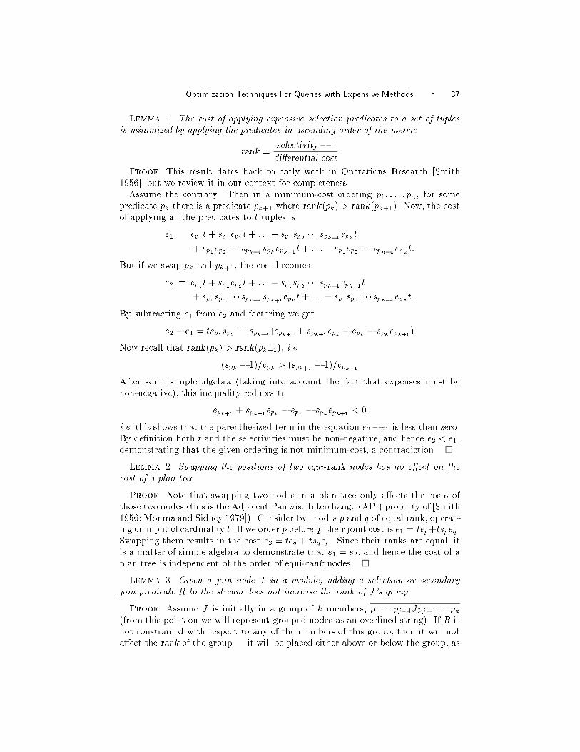
Optimization Techniques For Queries with Expensive Methods � 37
Lemma 1. The cost of applying expensive selection predicates to a set of tuples
is minimized by applying the predicates in ascending order of the metric
rank =selectivity� 1
di�erential cost
Proof. This result dates back to early work in Operations Research [Smith
1956], but we review it in our context for completeness.
Assume the contrary. Then in a minimum-cost ordering p1; : : : ; pn, for some
predicate pk there is a predicate pk+1 where rank(pk) > rank(pk+1). Now, the cost
of applying all the predicates to t tuples is
e1 = ep1t + sp1ep2 t+ : : :+ sp1sp2 � � �spk�1 epk t
+ sp1sp2 � � �spk�1 spkepk+1 t+ : : :+ sp1sp2 � � �spn�1 epn t:
But if we swap pk and pk+1, the cost becomes
e2 = ep1t + sp1ep2 t+ : : :+ sp1sp2 � � �spk�1 epk+1 t
+ sp1sp2 � � �spk�1 spk+1epk t+ : : :+ sp1sp2 � � �spn�1 epn t:
By subtracting e1 from e2 and factoring we get
e2 � e1 = tsp1sp2 � � �spk�1 (epk+1 + spk+1epk � epk � spkepk+1 )
Now recall that rank(pk) > rank(pk+1), i.e.
(spk � 1)=epk > (spk+1 � 1)=epk+1
After some simple algebra (taking into account the fact that expenses must be
non-negative), this inequality reduces to
epk+1 + spk+1epk � epk � spkepk+1 < 0
i.e. this shows that the parenthesized term in the equation e2� e1 is less than zero.
By de�nition both t and the selectivities must be non-negative, and hence e2 < e1,
demonstrating that the given ordering is not minimum-cost, a contradiction.
Lemma 2. Swapping the positions of two equi-rank nodes has no e�ect on the
cost of a plan tree.
Proof. Note that swapping two nodes in a plan tree only a�ects the costs of
those two nodes (this is the Adjacent Pairwise Interchange (API) property of [Smith
1956; Monma and Sidney 1979]). Consider two nodes p and q of equal rank, operat-
ing on input of cardinality t. If we order p before q, their joint cost is e1 = tep+tspeq .
Swapping them results in the cost e2 = teq + tsqep. Since their ranks are equal, it
is a matter of simple algebra to demonstrate that e1 = e2, and hence the cost of a
plan tree is independent of the order of equi-rank nodes.
Lemma 3. Given a join node J in a module, adding a selection or secondary
join predicate R to the stream does not increase the rank of J 's group.
Proof. Assume J is initially in a group of k members, p1 : : : pj�1Jpj+1 : : : pk
(from this point on we will represent grouped nodes as an overlined string). If R is
not constrained with respect to any of the members of this group, then it will not
a�ect the rank of the group | it will be placed either above or below the group, as
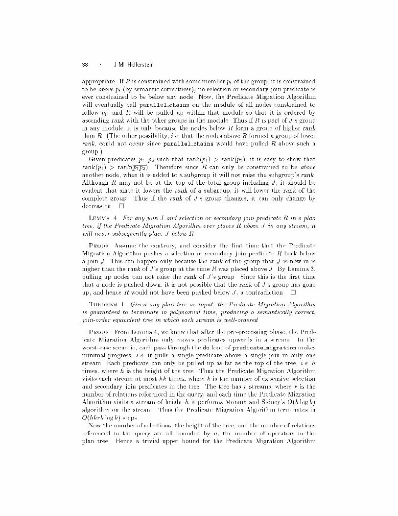
38 � J.M. Hellerstein
appropriate. If R is constrained with some member pi of the group, it is constrained
to be above pi (by semantic correctness); no selection or secondary join predicate is
ever constrained to be below any node. Now, the Predicate Migration Algorithm
will eventually call parallel chains on the module of all nodes constrained to
follow pi, and R will be pulled up within that module so that it is ordered by
ascending rank with the other groups in the module. Thus if R is part of J 's group
in any module, it is only because the nodes below R form a group of higher rank
than R. (The other possibility, i.e. that the nodes above R formed a group of lower
rank, could not occur since parallel chains would have pulled R above such a
group.)
Given predicates p1; p2 such that rank(p1) > rank(p2), it is easy to show that
rank(p1) > rank(p1p2). Therefore since R can only be constrained to be above
another node, when it is added to a subgroup it will not raise the subgroup's rank.
Although R may not be at the top of the total group including J , it should be
evident that since it lowers the rank of a subgroup, it will lower the rank of the
complete group. Thus if the rank of J 's group changes, it can only change by
decreasing.
Lemma 4. For any join J and selection or secondary join predicate R in a plan
tree, if the Predicate Migration Algorithm ever places R above J in any stream, it
will never subsequently place J below R.
Proof. Assume the contrary, and consider the �rst time that the Predicate
Migration Algorithm pushes a selection or secondary join predicate R back below
a join J . This can happen only because the rank of the group that J is now in is
higher than the rank of J 's group at the time R was placed above J . By Lemma 3,
pulling up nodes can not raise the rank of J 's group. Since this is the �rst time
that a node is pushed down, it is not possible that the rank of J 's group has gone
up, and hence R would not have been pushed below J , a contradiction.
Theorem 1. Given any plan tree as input, the Predicate Migration Algorithm
is guaranteed to terminate in polynomial time, producing a semantically correct,
join-order equivalent tree in which each stream is well-ordered.
Proof. From Lemma 4, we know that after the pre-processing phase, the Pred-
icate Migration Algorithm only moves predicates upwards in a stream. In the
worst-case scenario, each pass through the do loop of predicate migrationmakes
minimal progress, i.e. it pulls a single predicate above a single join in only one
stream. Each predicate can only be pulled up as far as the top of the tree, i.e. h
times, where h is the height of the tree. Thus the Predicate Migration Algorithm
visits each stream at most hk times, where k is the number of expensive selection
and secondary join predicates in the tree. The tree has r streams, where r is the
number of relations referenced in the query, and each time the Predicate Migration
Algorithm visits a stream of height h it performs Monma and Sidney's O(h logh)
algorithm on the stream. Thus the Predicate Migration Algorithm terminates in
O(hkrh logh) steps.
Now the number of selections, the height of the tree, and the number of relations
referenced in the query are all bounded by n, the number of operators in the
plan tree. Hence a trivial upper bound for the Predicate Migration Algorithm
Optimization Techniques For Queries with Expensive Methods � 39
is O(n4 logn). Note that this is a very conservative bound, which we present
merely to demonstrate that the Predicate Migration Algorithm is of polynomial
complexity. In general the Predicate Migration Algorithm should perform with
much greater e�ciency. After some number of steps in O(n4 logn), the Predicate
Migration Algorithm will have terminated, with each stream well-ordered subject
to the constraints of the given join order and semantic correctness.
Theorem 2. For every plan tree T1 there is a unique semantically correct, join-
order equivalent plan tree T2 with only well-ordered streams. Moreover, among all
semantically correct trees that are join-order equivalent to T1, T2 is of minimum
cost.
Proof. Theorem 1 demonstrates that for each tree there exists a semantically
correct, join-order equivalent tree of well-ordered streams (since the Predicate Mi-
gration Algorithm is guaranteed to terminate). To prove that the tree is unique,
we proceed by induction on the number of join nodes in the tree. Following the
argument of Lemma 2, we assume that all groups are of distinct rank; equi-rank
groups may be disambiguated via the IDs of the nodes in the groups.
Base case: The base case of zero join nodes is a simply a Scan node followed by
a series of selections, which can be uniquely ordered as shown in Lemma 1.
Induction Hypothesis: For any tree with k join nodes or less, there is a unique
semantically correct, join-order equivalent tree with well-ordered streams.
Induction: We consider two semantically correct, join-order equivalent plan trees,
T and T 0, each having k+1 join nodes and well-ordered streams. We will show that
these trees are identical, hence proving the uniqueness property of the theorem.
As illustrated in Figure 14, we refer to the uppermost join nodes of T and T0
as J and J0 respectively. We refer to the uppermost join or scan in the outer and
inner input streams of J as O and I respectively (O0 and I0 for J 0). We denote
the set of selections and secondary join predicates above a given join node p as
Rp, and hence we have, as illustrated, RJ above J , RJ 0 above J0, RO between O
and J , etc. We call a predicate in such a set mobile if there is a join below it in
the tree, and the predicate refers to the attributes of only one input to that join.
Mobile predicates can be moved below such joins without a�ecting the semantics
of the plan tree. First we establish that the subtrees O and O0 are identical. The
corresponding proof for I and I0 is analogous.
Consider a plan tree O+ composed of subtree O with a rank-ordered set RO+ of
predicates above it, where RO+ is made up of the union of RO and those predicates
of RJ that do not refer to attributes from I. If O and J are grouped together in
T , then let the cost and selectivity of O in O+ be modi�ed to include the cost and
selectivity of J . Consider an analogous tree O+0, with RO+0 being composed of
the union of RO0 and those predicates of RJ 0 that do not refer to I0. Modify the
cost and selectivity of O0 in O+0 as before. It should be clear that O+ and O
+0
are join-order equivalent trees of less than k nodes. Since T and T0 are assumed
to have well-ordered streams, then clearly so do O and O0. Hence by the induction
hypothesis O+ and O
+0 are identical, and therefore the subtrees O and O0 are
identical.
Thus the only di�erences between T and T0 must occur above O; I;O0
; and I0.
Now since the sets of predicates in the two trees are equal, and since O and O0, I
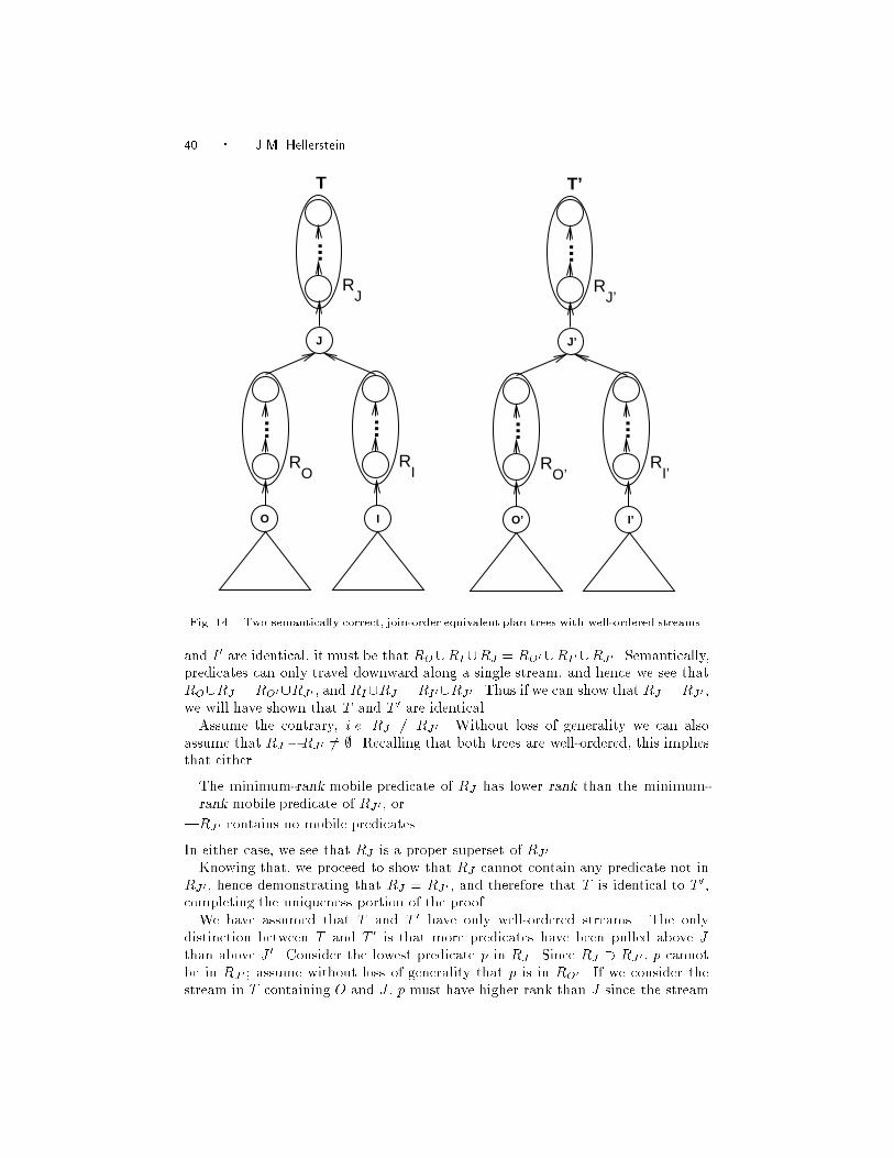
40 � J.M. Hellerstein
RJ
...
T
J
O I
R
...
R
...
O I
R
...
R
...
R
...
T’
J’
J’
O’
O’ I’
I’
Fig. 14. Two semantically correct, join-order equivalent plan trees with well-ordered streams.
and I0 are identical, it must be that RO[RI [RJ = RO0 [RI0[RJ 0. Semantically,
predicates can only travel downward along a single stream, and hence we see that
RO[RJ = RO0[RJ 0 , and RI[RJ = RI0[RJ 0 . Thus if we can show that RJ = RJ 0 ,
we will have shown that T and T0 are identical.
Assume the contrary, i.e. RJ 6= RJ 0 . Without loss of generality we can also
assume that RJ �RJ 0 6= ;. Recalling that both trees are well-ordered, this implies
that either
|The minimum-rank mobile predicate of RJ has lower rank than the minimum-
rank mobile predicate of RJ 0 , or
|RJ 0 contains no mobile predicates.
In either case, we see that RJ is a proper superset of RJ 0 .
Knowing that, we proceed to show that RJ cannot contain any predicate not in
RJ 0 , hence demonstrating that RJ = RJ 0 , and therefore that T is identical to T0,
completing the uniqueness portion of the proof.
We have assumed that T and T0 have only well-ordered streams. The only
distinction between T and T0 is that more predicates have been pulled above J
than above J 0. Consider the lowest predicate p in RJ . Since RJ � RJ 0 , p cannot
be in RJ 0 ; assume without loss of generality that p is in RO0 . If we consider the
stream in T containing O and J , p must have higher rank than J since the stream
Optimization Techniques For Queries with Expensive Methods � 41
is well-ordered and p is mobile { i.e., if p had lower rank than J it would be below
J . Further, J must be in a group by itself in this stream, since p is directly above
J and of higher rank than J . Now, consider the stream in T0 containing O0 and J
0.
In this stream, J 0 can have rank no greater than the rank of J , since J is in a group
by itself and Lemma 3 tells us that adding nodes to a group can only lower the
group's rank. Since p has higher rank than J , and the rank of J 0 is no higher than
that of J , p must have higher rank than J 0. This contradicts our earlier assumption
that T 0 is well-ordered, and hence it must be that T and T0 were identical to begin
with; i.e. there is only one unique tree with well-ordered streams.
It is easy to see that a minimum-cost tree is well-ordered, and hence that some
well-ordered tree has minimum cost. Assume the contrary, i.e. there is a semanti-
cally correct, join-order equivalent tree T of minimum cost that has a stream that
is not well ordered. Then in this stream there is a group v adjacent to a group
w such that v and w are not well-ordered, and v and w may be swapped without
violating the constraints. Since swapping the order of these two groups a�ects only
the cost of the nodes in v and w, the total cost of T can be made lower by swapping
v and w, contradicting our assumption that T was of minimum cost.
Since T2 is the only semantically correct tree of well-ordered streams that is join-
order equivalent to T1, it follows that T2 is of minimum cost. This completes the
proof.
Lemma 5. For a selection or secondary join predicate R in a subexpression, if
the rank of R is greater than the rank of any join in any plan for the subexpression,
then in the optimal complete tree R will appear above the highest join in a subtree
for the subexpression.
Proof. Recall that rank(p1) > rank(p1p2). Thus in any full plan tree T con-
taining a subtree T0 for the subexpression, the highest-rank group containing nodes
from T0 will be of rank less than or equal to the rank of the highest-rank join node
in T0. A selection or secondary join predicate of higher rank than the highest-rank
join node of T0 is therefore certain to be placed above T0 in T .
Recommended


![[Lars Erik Persson, Etc.] the Homogenization Metho(BookSee.org)](https://img.pdfslide.us/doc/110x75/5695cfe31a28ab9b028ff65d/lars-erik-persson-etc-the-homogenization-methobookseeorg.jpg)