QUASIPARTICLES AND VORTICES IN THE HIGH
TEMPERATURE CUPRATE SUPERCONDUCTORS
by
Oskar Vafek
A dissertation submitted to The Johns Hopkins University in conformity with the
requirements for the degree of Doctor of Philosophy.
Baltimore, Maryland
August, 2003
c© Oskar Vafek 2003
All rights reserved
Abstract
In this thesis I present a study of the interplay of vortices and the fermionic quasi-
particle states in a quasi 2-dimensional d-wave superconductors, such as high temper-
ature cuprate superconductors. In the first part, I start by analyzing the quasiparticle
states in the presence of the magnetic field induced vortex lattice. Unlike in the s-
wave superconductor, there are no vortex bound states, rather all the quasiparticle
states are extended. By using general arguments based on symmetry principles and
by direct (numerical) computation, I show that these extended quasiparticle states
are gapped. In addition, they are characterized by a topological invariant with regard
to their spin Hall conduction. Finally, I relate the spin Hall conductivity tensor σspinxy
to the thermal Hall conductivity κxy by deriving the appropriate “Wiedemann-Franz”
law. In the second part, I analyze the fluctuations around an ordered d-wave super-
conductor (in the absence of the external magnetic field), focusing on the interaction
between the low energy nodal fermions and the vortex-antivortex phase excitations.
It is shown that the corresponding low energy effective theory for the nodal fermions
in the normal (non-superconducting) state is QED3 or quantum electrodynamics in
2+1 space time dimensions. The massless U(1) gauge field encodes the topological
interaction between the quasiparticles and the hc/2e vortices at long wavelengths.
I analyze the symmetries, correlations and stability of this state. In particular, I
study the role of Dirac cone anisotropy and residual interactions in QED3 as well as
the physical meaning of the chiral symmetry breaking. Remarkably, the spin density
wave corresponds to an instability of a phase fluctuating d-wave superconductor.
Advisor: Zlatko B. Tesanovic.
ii
iii
Acknowledgements
I wish to express my deep gratitude to Prof. Zlatko Tesanovic for sharing his
insights and library of knowledge with me, and for constant and uncompromising
quest for the profound that he inspires.
I also wish to thank Ashot Melikyan for many invaluable discussions and debates,
and for his exceptional selflessness in helping me and others.
iv
Contents
Abstract ii
Acknowledgements iv
List of Figures vii
1 Introduction 11.1 Phenomenology of High Temperature Cuprate Superconductors . . . 3
2 Quasiparticles in the mixed state of HTS 92.1 Introduction . . . . . . . . . . . . . . . . . . . . . . . . . . . . . . . . 92.2 Quasiparticle excitation spectrum of a d-wave superconductor in the
mixed state . . . . . . . . . . . . . . . . . . . . . . . . . . . . . . . . 162.2.1 Particle-Hole Symmetry . . . . . . . . . . . . . . . . . . . . . 192.2.2 Franz-Tesanovic Transformation and Translation Symmetry . 192.2.3 Vortex Lattice Inversion Symmetry and Level Crossing . . . . 22
2.3 Topological quantization of spin and thermal Hall conductivities . . . 252.3.1 Spin Conductivity . . . . . . . . . . . . . . . . . . . . . . . . . 262.3.2 Thermal Conductivity . . . . . . . . . . . . . . . . . . . . . . 31
2.4 Discussion and Conclusion . . . . . . . . . . . . . . . . . . . . . . . . 33
3 QED3 theory of the phase disordered d-wave superconductors 363.1 Introduction . . . . . . . . . . . . . . . . . . . . . . . . . . . . . . . . 363.2 Vortex quasiparticle interaction . . . . . . . . . . . . . . . . . . . . . 38
3.2.1 Protectorate of the pairing pseudogap . . . . . . . . . . . . . . 383.2.2 Topological frustration . . . . . . . . . . . . . . . . . . . . . . 393.2.3 “Coarse-grained” Doppler and Berry U(1) gauge fields . . . . 433.2.4 Further remarks on FT gauge . . . . . . . . . . . . . . . . . . 463.2.5 Maxwellian form of the Jacobian L0[vµ, aµ] . . . . . . . . . . . 48
3.3 Low energy effective theory . . . . . . . . . . . . . . . . . . . . . . . 553.3.1 Effective Lagrangian for the pseudogap state . . . . . . . . . . 583.3.2 Berryon propagator . . . . . . . . . . . . . . . . . . . . . . . . 60
v

3.3.3 TF self energy and propagator . . . . . . . . . . . . . . . . . . 623.4 Effects of Dirac anisotropy in symmetric QED3 . . . . . . . . . . . . 64
3.4.1 Anisotropic QED3 . . . . . . . . . . . . . . . . . . . . . . . . 653.4.2 Gauge field propagator . . . . . . . . . . . . . . . . . . . . . . 663.4.3 TF self energy . . . . . . . . . . . . . . . . . . . . . . . . . . . 693.4.4 Dirac anisotropy and its β function . . . . . . . . . . . . . . . 70
3.5 Finite temperature extensions of QED3 . . . . . . . . . . . . . . . . . 723.5.1 Specific heat and scaling of thermodynamics . . . . . . . . . . 753.5.2 Uniform spin susceptibility . . . . . . . . . . . . . . . . . . . . 76
3.6 Chiral symmetry breaking . . . . . . . . . . . . . . . . . . . . . . . . 783.7 Summary and conclusions . . . . . . . . . . . . . . . . . . . . . . . . 85
A Quasiparticle correlation functions in the mixed state 87A.1 Green’s functions: definitions and identities . . . . . . . . . . . . . . 87A.2 Spin current and spin conductivity tensor . . . . . . . . . . . . . . . . 89A.3 Thermal current and thermal conductivity tensor . . . . . . . . . . . 91
B Field theory of quasiparticles and vortices 98B.1 Jacobian L0 . . . . . . . . . . . . . . . . . . . . . . . . . . . . . . . . 98
B.1.1 2D thermal vortex-antivortex fluctuations . . . . . . . . . . . 98B.1.2 Quantum fluctuations of (2+1)D vortex loops . . . . . . . . . 101
B.2 Feynman integrals in QED3 . . . . . . . . . . . . . . . . . . . . . . . 106B.2.1 Vacuum polarization bubble . . . . . . . . . . . . . . . . . . . 106B.2.2 TF self energy: Lorentz gauge . . . . . . . . . . . . . . . . . . 107
B.3 Feynman integrals for anisotropic case . . . . . . . . . . . . . . . . . 108B.3.1 Self energy . . . . . . . . . . . . . . . . . . . . . . . . . . . . . 108
B.4 Physical modes of a finite T QED3 . . . . . . . . . . . . . . . . . . . 110B.5 Finite Temperature Vacuum Polarization . . . . . . . . . . . . . . . . 113B.6 Free energy scaling of QED3 . . . . . . . . . . . . . . . . . . . . . . . 118
Bibliography 120
Vita 127
vi

List of Figures
1.1 (A) The unit cell of La2−xSrxCuO4 family of high temperature super-conductors. It is believed that most of the interesting physics happensin the Cu-O2 plane, which extends in the a− b directions. The c−axiselectronic coupling is very small. In this family of materials, doping isachieved by replacing some of the La atoms for Sr, or by adding in-terstitial oxygen atoms. This crystalline structure is slightly modifiedin different high-Tc cuprates, but all share the weakly coupled Cu-O2
planes. (B) Arrows indicate spin alignment in the antiferromagenticstate, the parent state of HTS. (Taken from [3]) . . . . . . . . . . . . 4
1.2 Phase diagram of electron and hole doped High Temperature super-conductors showing the superconducting (SC), antiferromagnetic (AF),pseudogap and metallic phases. (Taken from [4]). . . . . . . . . . . . 5
1.3 The magnetic flux threading through a polycrystalline YBCO ring,monitored with a SQUID magnetometer as a function of time. The fluxjumps occur in integral multiples of the superconducting flux quantumΦ0 = hc/2e. This experiment demonstrates that the superconductivityin high temperature cuprates is due to Cooper pairing. (taken from [5]) 6
1.4 The pairing gap of HTS has dx2−y2-wave symmetry (left). The pointson the Fermi surface at which the gap disappears (the nodal points)can be identified in the angle resolved photoemission spectra (right) [4]. 7
1.5 Contours of the constant Nernst coefficient in the Temperature vs. dop-ing phase diagram. The units of the Nernst coefficient are nanoVolt perKelvin per Tesla. At low temperature and in the strongly underdopedregion the Nernst signal is almost three orders of magnitude greaterthan it would be in a normal metal. Such a large signal is typicallyobserved in the vortex liquid state, where it is associated with Joseph-son phase-slips produced across the sample due to thermally diffusingvortices. In this experiment, however, this signal is seen several tensof Kelvins above the superconducting transition temperature Tc! [8] 8
vii

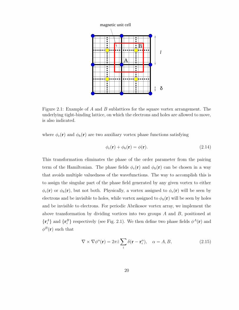
2.1 Example of A and B sublattices for the square vortex arrangement.The underlying tight-binding lattice, on which the electrons and holesare allowed to move, is also indicated. . . . . . . . . . . . . . . . . . . 20
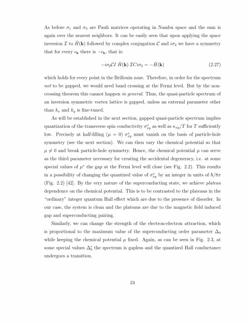
2.2 The mechanism for changing the quantized spin Hall conductivity isthrough exchanging the topological quanta via (“accidental”) gap clos-ing. The upper panel displays spin Hall conductivity σsxy as a functionof the chemical potential µ. The lower panel shows the magnetic fieldinduced gap ∆m in the quasiparticle spectrum. Note that the changein the spin Hall conductivity occurs precisely at those values of chem-ical potential at which the gap closes. Hence the mechanism behindthe changes of σsxy is the exchange of the topological quanta at theband crossings. The parameters for the above calculation were: squarevortex lattice, magnetic length l = 4δ, ∆ = 0.1t or equivalently theDirac anisotropy αD = 10. . . . . . . . . . . . . . . . . . . . . . . . . 25
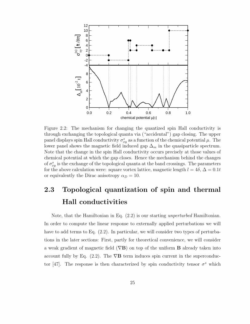
2.3 The upper panel displays spin Hall conductivity σsxy as a function ofthe maximum superconducting order parameter ∆0. The lower panelshows the magnetic field induced gap in the quasiparticle spectrum.The change in the spin Hall conductivity occurs at those values of ∆0
at which the gap closes. The parameters for the above calculation were:square vortex lattice, magnetic length l = 4δ, µ = 2.2t. . . . . . . . . 26
3.1 Schematic representation of the Fermi surface of the cuprate supercon-ductors with the indicated nodal points of the dx2−y2 gap. . . . . . . . 56
3.2 One loop Berryon polarization (a) and TF self energy (b). . . . . . . 613.3 The RG β-function for the Dirac anisotropy in units of 8/3π2N . The
solid line is the numerical integration of the quadrature in the Eq.(B.52) while the dash-dotted line is the analytical expansion aroundthe small anisotropy (see Eq. (3.92-3.94)). At αD = 1, βαD
crosses zerowith positive slope, and therefore at large length-scales the anisotropicQED3 scales to an isotropic theory. . . . . . . . . . . . . . . . . . . . 73
3.4 Schematic phase diagram of a cuprate superconductor in QUT. De-pending on the value of Nc (see text), either the superconductor isfollowed by a symmetric phase of QED3 which then undergoes a quan-tum CSB transition at some lower doping (panel a), or there is a directtransition from the superconducting phase to the mch 6= 0 phase ofQED3 (panel b). The label SDW/AF indicates the dominance of theantiferromagnetic ground state as x → 0. . . . . . . . . . . . . . . . 80
3.5 The “Fermi surface” of cuprates, with the positions of nodes in thed-wave pseudogap. The wavectors Q11,Q22,Q12, etc. are discussed inthe text. . . . . . . . . . . . . . . . . . . . . . . . . . . . . . . . . . 81
viii

Chapter 1
Introduction
The properties of matter at low temperature amplify nature’s most fascinating
and least comprehensible laws: the laws of quantum mechanics. This amplification
process occurs via a principle of symmetry breaking: when the available phase space
is sufficiently restricted, interacting systems with a macroscopically large number of
degrees of freedom tend to seek a highly organized state. In other words, the low
energy state of a many particle system possesses less symmetry than the laws which
are obeyed by its constituents. A commonplace example are solids. Despite the
fact that the laws of quantum mechanics are invariant under spatial translation, the
atoms in a solid occupy a regular array which is only disrupted by small amplitude
vibrations and occasional dislocation defects. It is the translational symmetry that
is broken by the solid state of matter. This symmetry breaking has an important
ramification: the emergence of Goldstone modes, or long lived degrees of freedom,
which tend to restore the symmetry. In the case of a solid, this is embodied by the
emergence of transverse elastic waves. In addition, symmetry breaking generally leads
to stable topological defects; in solids these are lattice dislocations and disclinations.
While such topological defects are quite rare deep inside an ordered state, they can
be crucial in destroying the order near a phase transition.
A less commonplace example of symmetry breaking is a superconductor. While
the laws of quantum mechanics are invariant under a local U(1) transformation, i.e.
multiplication of the wavefunction by a space dependent single valued phase factor,
1
the superconducting state is not. In a superconductor the many body wavefunction
acquires rigidity under a phase twist. This leads to most of the fascinating proper-
ties of superconductors such as the passage of current without any voltage drop, the
Meissner effect, or even the magnetic levitation. The density of low energy fermionic
excitations is generically appreciably reduced compared to the non-superconducting
state. The Goldstone mode that accompanies the symmetry breaking corresponds to
smooth (longitudinal) space-time variations of the phase of the many body wavefunc-
tion. On the other hand, 2π phase twists of the wavefunction, or vortices, are the
analog of the dislocations in the solid. They form the topological defects in the type-II
superconductors. At a phase transition, temperature T = Tc, such a superconductor
looses its phase rigidity due to the free motion of vortex defects. The temperature
interval around Tc in which this physics applies is typically barely detectable in the
conventional low Tc superconductors, but there is growing experimental evidence
that in the high Tc cuprate superconductors (HTS) vortex unbinding is the dominant
mechanism of the loss of long range order. In particular, the underdoped materials
appear to exhibit many characteristics associated with vortex physics, in some cases
all the way down to zero temperature! Such observations suggest that the quantum
analog of vortex unbinding occurs at the superconductor-insulator quantum phase
transition.
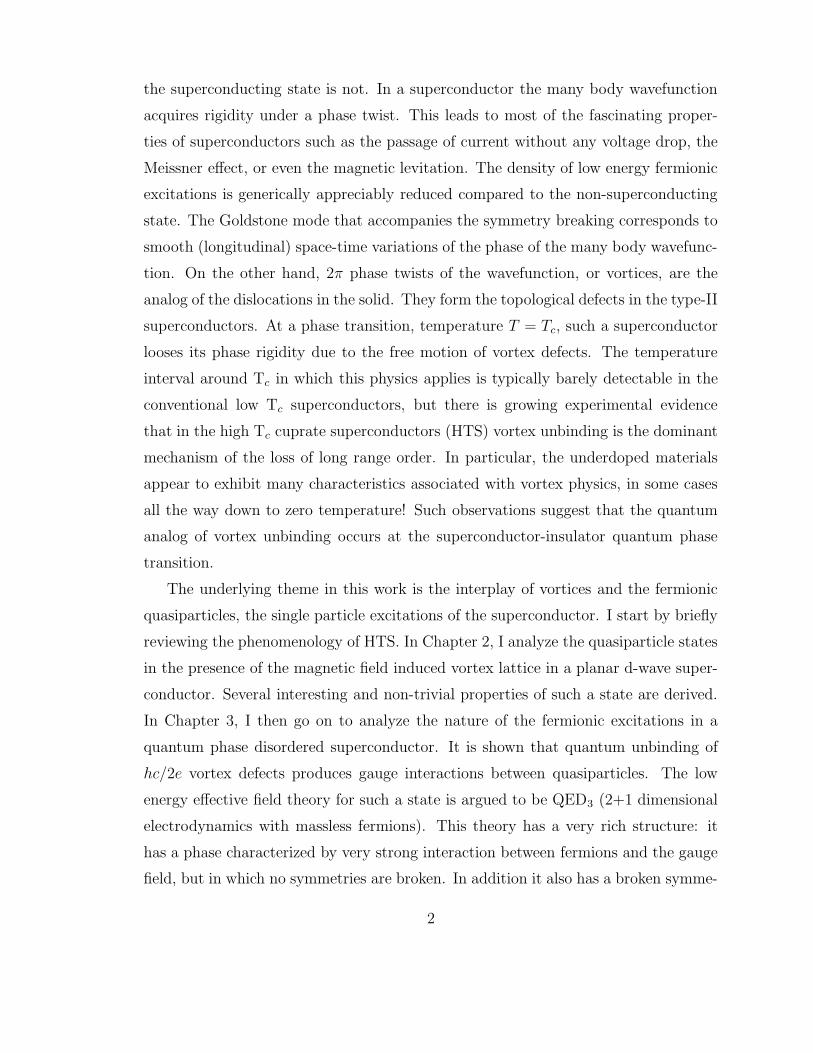
The underlying theme in this work is the interplay of vortices and the fermionic
quasiparticles, the single particle excitations of the superconductor. I start by briefly
reviewing the phenomenology of HTS. In Chapter 2, I analyze the quasiparticle states
in the presence of the magnetic field induced vortex lattice in a planar d-wave super-
conductor. Several interesting and non-trivial properties of such a state are derived.
In Chapter 3, I then go on to analyze the nature of the fermionic excitations in a
quantum phase disordered superconductor. It is shown that quantum unbinding of
hc/2e vortex defects produces gauge interactions between quasiparticles. The low
energy effective field theory for such a state is argued to be QED3 (2+1 dimensional
electrodynamics with massless fermions). This theory has a very rich structure: it
has a phase characterized by very strong interaction between fermions and the gauge
field, but in which no symmetries are broken. In addition it also has a broken symme-
2

try phase in which the fermions gain mass. Remarkably, this state can be associated
with a spin density wave, a state adiabatically connected to an antiferromagnet, the
parent state of all cuprate superconductors.
1.1 Phenomenology of High Temperature Cuprate
Superconductors
High temperature cuprate superconductors were discovered by Bednorz and Muller
in 1986 [1]. Soon thereafter, Anderson pointed out three essential features of the new
materials [2]. First, they are quasi 2-dimensional with weakly coupled CuO2 planes
(Fig. 1.1). Second, the superconductor is created by doping a Mott insulator, and
third, Anderson proposed that the combination of proximity to a Mott insulator and
low dimensionality would cause the doped material to exhibit fundamentally new
behavior, impossible to explain by conventional paradigms of metal physics [2, 3].
In a Mott insulator, charge transport is prohibited not merely by the Pauli exclu-
sion principle (as in a band insulator), but also by strong electron-electron repulsion
that pins the electrons to the lattice sites. This insulating state is stable when there
is exactly one electron per each site in the valence band, since motion of electrons re-
quires energetically expensive double occupancy. Virtual charge excitations generate
a ”super-exchange” interaction that favors antiferromagnetic alignment of spins (Fig.
1.1).
Upon doping, the system becomes a weak conductor and eventually a super-
conductor, Fig. (1.2). However, the cuprates are the only Mott insulators which
become superconducting when doped [3]. It was established soon after the discovery
of HTS that the superconductivity is due to the electrons forming Cooper pairs (see
Fig. 1.3). However, unlike in conventional s-wave superconductors, the gap function
changes sign upon 90 degree rotation i.e. it has dx2−y2 symmetry. As such, it vanishes
at four points on the Fermi surface, leading to gapless Fermi points. These points
were identified by angle–resolved photoemission spectroscopy (ARPES) (Fig. 1.4). In
addition, several ingenious phase sensitive tests, based on Josephson tunneling, were
3

Figure 1.1: (A) The unit cell of La2−xSrxCuO4 family of high temperature super-conductors. It is believed that most of the interesting physics happens in the Cu-O2
plane, which extends in the a − b directions. The c−axis electronic coupling is verysmall. In this family of materials, doping is achieved by replacing some of the Laatoms for Sr, or by adding interstitial oxygen atoms. This crystalline structure isslightly modified in different high-Tc cuprates, but all share the weakly coupled Cu-O2 planes. (B) Arrows indicate spin alignment in the antiferromagentic state, theparent state of HTS. (Taken from [3])
developed to demonstrate the change of sign of the pairing amplitude (for a review
see [5]). The low energy properties of such d-wave superconductors are governed by
the excitations around the four nodal points. These correspond to nodal BCS quasi-
particles whose existence was demonstrated by several techniques, but most directly
by ARPES. These low energy BCS quasiparticles are responsible, for example, for the
linear in temperature depletion of superfluid density [6] or ”universal” longitudinal
thermal conductivity, which was demonstrated experimentally [7] to depend only on
the ratio of the quasiparticle velocity perpendicular and parallel to the Fermi surface
at the Fermi points.
The boundary in the phase diagram between the antiferromagnet and the super-
conductor corresponds to a fascinating phase: the pseudogap state. This state is not
a superconductor, but spectroscopically it is nearly indistinguishable from the super-
conductor as there is a suppression of single particle states at the Fermi surface as
well as the nodal points. While the spin fluctuations are gapped, the in-plane charge
4

Figure 1.2: Phase diagram of electron and hole doped High Temperature supercon-ductors showing the superconducting (SC), antiferromagnetic (AF), pseudogap andmetallic phases. (Taken from [4]).
transport seems unaffected, whereas the c-axis transport is suppressed. Moreover,
strong superconducting fluctuations seem to be prominent in this state. Especially
striking are the recent observations of anomalously large Nernst signal [8] above Tc in
single crystal underdoped cuprates (see Fig. 1.5). In this measurement, a magnetic
field is applied perpendicular to the CuO2 planes, along with a weak thermal gradi-
ents within the plane. One then measures the electrical voltage drop perpendicular to
the thermal current flow. The signal seen is nearly three orders of magnitude larger
than in conventional metals, not unlike in vortex liquid state. However, it is observed
several tens on Kelvin above Tc! This suggests that the physics of pseudogap is
dominated by strong pairing fluctuations.
In what follows, I shall first study the BCS quasiparticles of a d-wave supercon-
ductor with magnetic field induced array of Abrikosov vortices. I shall assume that we
are at T = 0 far away from any phase transition so that fluctuations can be neglected
(e.g. the region between optimally doped and slightly overdoped in the phase dia-
gram (1.2)). Later, I shall concentrate on the pseudogap region, and assume that it is
dominated by phase fluctuations, in particular that the pseudogap region is nothing
5
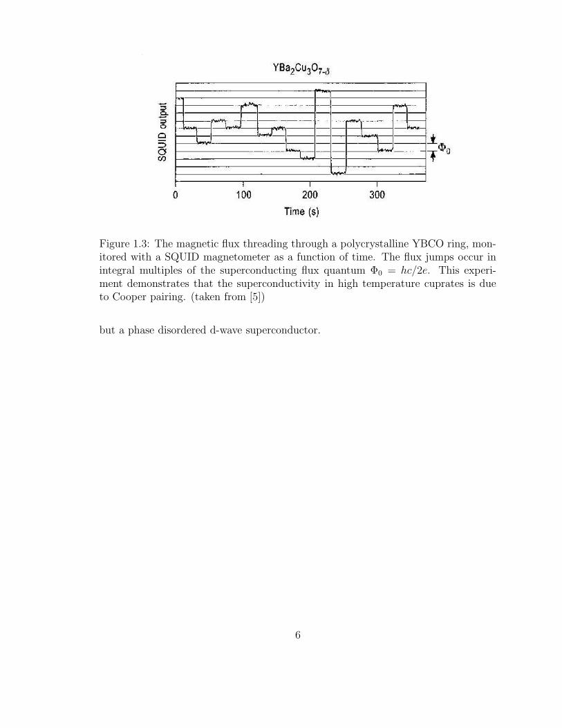
Figure 1.3: The magnetic flux threading through a polycrystalline YBCO ring, mon-itored with a SQUID magnetometer as a function of time. The flux jumps occur inintegral multiples of the superconducting flux quantum Φ0 = hc/2e. This experi-ment demonstrates that the superconductivity in high temperature cuprates is dueto Cooper pairing. (taken from [5])
but a phase disordered d-wave superconductor.
6
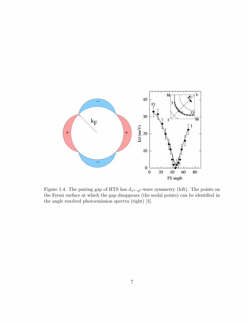
−
−
+ +
kF
Figure 1.4: The pairing gap of HTS has dx2−y2-wave symmetry (left). The points onthe Fermi surface at which the gap disappears (the nodal points) can be identified inthe angle resolved photoemission spectra (right) [4].
7

1.0 0.8 0.6 0.4 0.2 0.00
20
40
60
80
100
120
1000
200
Bi2Sr
2-yLa
yCuO
6
20
400100
40
10nV/KT
Tonset
Tc
T (
K)
La content y
Figure 1.5: Contours of the constant Nernst coefficient in the Temperature vs. dopingphase diagram. The units of the Nernst coefficient are nanoVolt per Kelvin per Tesla.At low temperature and in the strongly underdoped region the Nernst signal is almostthree orders of magnitude greater than it would be in a normal metal. Such a largesignal is typically observed in the vortex liquid state, where it is associated withJosephson phase-slips produced across the sample due to thermally diffusing vortices.In this experiment, however, this signal is seen several tens of Kelvins above thesuperconducting transition temperature Tc! [8]
8

Chapter 2
Quasiparticles in the mixed state
of HTS
2.1 Introduction
In this section we give a brief review of the fermionic quasiparticle excitations in
the superconductors, both conventional and unconventional.
In conventional (s-wave) superconductors the effective attraction between elec-
trons is mainly due to exchange of phonons [9]. The evidence of the phonon mediated
interaction comes from the isotope effect i.e. the shift of the transition temperature
upon the replacement of the crystal ions with their isotopes. The electrons pair in
the lowest angular momentum channel, l = 0 or s-wave, and the pairing amplitude
does not vary appreciably around the Fermi surface. As a result, the single parti-
cle fermionic excitations (quasiparticles) are fully gapped everywhere on the Fermi
surface and the quasiparticle density of states vanishes below a specific energy. This
has profound consequences for the traditional phenomenology of superconductors.
The gap in the fermionic spectrum leads to the well known activated form of the
quasiparticle contribution to various thermodynamic and transport properties, and
can be directly observed in tunneling spectroscopy (see e.g. [5]). Furthermore, even
beyond the mean-field theory, the presence of the pairing gap in the superconducting
state cuts off the infra-red singularities which allows perturbative treatment of various
9

types of quasiparticle interactions.
High temperature cuprate superconductors (HTS), however, are different. While
the origin of pairing remains an unsolved problem, the cuprates appear to be accu-
rately described by the dx2−y2-wave order parameter [10], i.e. the pairing happens
in l = 2 channel whose degeneracy is further split by the crystal field in favor of
dx2−y2 . As a result, quasiparticle excitations occur at arbitrarily low energy near the
nodal points. These low energy fermionic excitations appear to govern much of the
thermodynamics and transport in the HTS materials. This represents a new intel-
lectual challenge [11]: one must devise methods that can incorporate the low energy
fermionic excitations into the phenomenology of superconductors, both within the
mean-field BCS-like theory and beyond.
This challenge is not trivial and has many diverse components. Low energy qua-
siparticles are scattered by impurities in novel and unusual ways, depending on the
low energy density of states [12]. They interact with external perturbations in ways
not encountered in conventional superconductors, and these interactions give rise to
new phenomena [13, 14]. The low energy quasiparticles are thus expected to qual-
itatively affect the quantum critical behavior of HTS (see Chapter 3). Among the
many aspects of this new quasiparticle phenomenology a particularly prominent role
is played by the low lying quasiparticle excitations in the mixed (or vortex) state [15].
All HTS are extreme type-II systems and have a huge mixed phase extending from
the lower critical field Hc1 which is in the range of 10-100 Gauss to the upper critical
field Hc2 which can be as large as 100-200 T. In this large region the interactions
between quasiparticles and vortices play the essential role in defining the nature of
thermodynamic and transport properties.
Thermodynamic and transport properties are expected to be rather different for
distinct classes of unconventional superconductors. The difference stems from a com-
plex motion of the quasiparticles under the combined effects of both the magnetic
field B and the local drift produced by chiral supercurrents of the vortex state. For
example, in HTS the dx2−y2-wave nature of the gap function results in its vanishing
along nodal directions. Along these nodal directions the pair-breaking induced by
supercurrents has a particularly strong effect. On the other hand, in unconventional
10

superconductors with the px±iy pairing, Sr2RuO4 being a possible candidate [16], the
spectrum is fully gapped but the order parameter is chiral even in the absence of
external magnetic field. This leads to two different types of vortices for two different
field orientations [17, 18].
Still, in all these different situations, the quantum dynamics of quasiparticles
in the vortex state contains two essential common ingredients. First, there is the
purely classical effect of the Doppler shift [13, 14]: quasiparticles’ energy is shifted
by a locally drifting superfluid, E(k) → E(k) − ~vs(r) · k, where vs(r) is the local
superfluid velocity. vs(r) contains information about vortex configurations, allowing
us to connect quasiparticle spectral properties to various cooperative phenomena in
the system of vortices [19, 20, 21]. The Doppler shift effect is not peculiar to the vortex
state. It also occurs in the Meissner phase [14] and is generally present whenever a
quasiparticle experiences a locally uniform drift in the superfluid velocity. Second,
there is also a purely quantum effect which is intimately tied to the vortex state:
as a quasiparticle circles around a vortex while maintaining its quantum coherence,
the accumulated phase through a Doppler shift is ±π. This implies that there must
be an additional compensating ±π contribution to the phase on top of the one due
to the Doppler shift in order for the wavefunction to remain single-valued [22]. The
required ±π contribution is supplied by a “Berry phase” effect and can be built in at
the Hamiltonian level as a half-flux Aharonov-Bohm scattering of quasiparticles by
vortices [22]. This interplay between the classical (Doppler shift) and purely quantum
effect (“Berry phase”) is what makes the problem of quasiparticle-vortex interaction
particularly fascinating.
Let us briefly review what is already known about the quasiparticles in the vortex
state. The initial theoretical investigations of gapped and gapless superconductors
in the vortex state were directed along rather separate lines. The low energy qua-
siparticle spectrum of an s-wave superconductor in the mixed state was originally
studied by Caroli, de Gennes and Matricon (CdGM) [23] within the framework of the
Bogoliubov-de Gennes equations [24]. Their solution yields well known bound states
in the vortex cores. These states are localized in the core and have an exponential
envelope, the scale of which is set by the BCS coherence length. The low energy
11
end of the spectrum is given by εµ ∼ µ(∆20/EF ), where µ = 1/2, 3/2, . . . , ∆0 is the
overall BCS gap, and EF is the Fermi energy. This solution can be relatively straight-
forwardly generalized to a fully gapped, chiral p-wave superconductor. In this case
the low energy quasiparticle spectrum also displays bound vortex core states, whose
energy quantization is, however, modified relative to its s-wave counterpart, precisely
because of the chiral character of a px±iy-wave superconductor and the ensuing shift
in the angular momentum. For example, the low energy spectrum of quasiparticles
in the singly quantized vortex of the px±iy-wave superconductor, possesses a state at
exactly zero energy [17, 18].
By comparison, the spectrum of a gapless d-wave superconductor in the mixed
phase has become the subject of an active debate only relatively recently, fueled by
the interest in HTS. Naturally, the first question that arises is what is the analog
of the CdGM solution for a single vortex. It is important to realize here that the
situation in a dx2−y2 superconductor is qualitatively different from the classic s-wave
case [25]: when the pairing state has a finite angular momentum and is not a global
eigenstate of the angular momentum Lz (a dx2−y2 superconductor is an equal ad-
mixture of Lz = ±2 states), the problem of fermionic excitations in the core cannot
be reduced to a collection of decoupled 1D dimensional eigenvalue equations for each
angular momentum channel, the key feature of the CdGM solution. Instead, all chan-
nels remain coupled and one must solve a full 2D problem. The fully self-consistent
numerical solution of the BdG equations [25, 26] reveals the most important physical
consequence of this qualitatively new situation: the vortex core quasiparticle states in
a pure dx2−y2 superconductor are delocalized with wave functions extended along the
nodal directions. The low lying states have a continuous spectrum and, in a broad
range of parameters, do not seem to exhibit strong resonant behavior. This is in
sharp contrast with a discrete spectrum and true bound quasiparticle states of the
CdGM s-wave solution.
A particularly important issue in this context is the nature of the quasiparticle
excitations at very low fields, in the presence of a vortex lattice. This is a novel
challenge since the spectrum starts as gapless at zero field and at issue is the inter-
action of these low lying quasiparticles with the vortex lattice. This problem has
12
been addressed via numerical solution of the tight binding model [27], a numerical
diagonalization of the continuum model [28] and a semiclassical analysis [13]. Gorkov,
Schrieffer [29] and, in a somewhat different context, Anderson [61], predicted that the
quasiparticle spectrum is described by a Dirac-like Landau quantization of energy
levels
En = ±~ωH√n, n = 0, 1, ... (2.1)
where ωH =√
2ωc∆0/~, ωc = eB/mc is the cyclotron frequency and ∆0 is the
maximum superconducting gap. The Dirac-like spectrum of Landau levels arises from
the linear dispersion of nodal quasiparticles at zero field. This argument neglects the
effect of spatially varying supercurrents in the vortex array which were shown to
strongly mix individual Landau levels [31].
Recently, Franz and Tesanovic (FT) [22] pointed out that the low energy quasi-
particle states of a dx2−y2-wave superconductor in the vortex state are most naturally
described by strongly dispersive Bloch waves. This conclusion was based on the par-
ticular choice of a singular gauge transformation, which allows for the treatment of
the uniform external magnetic field and the effects produced by chiral supercurrents
on equal footing. The starting point was the Bogoliubov-de Gennes (BdG) equation
linearized around a Dirac node. By employing the singular gauge transformation FT
mapped the original problem onto that of a Dirac Hamiltonian in periodic vector
and scalar potentials, comprised of an array of an effective magnetic Aharonov-Bohm
half-fluxes, and with a vanishing overall magnetic flux per unit cell. The FT gauge
transformation allows use of standard band structure and other zero-field techniques
to study the quasiparticle dynamics in the presence of vortex arrays, ordered or disor-
dered. Its utility was illustrated in Ref. [22] through computation of the quasiparticle
spectra of a square vortex lattice. A remarkable feature of these spectra is the per-
sistence of the massless Dirac node at finite fields and the appearance of the “lines
of nodes” in the gap at large values of the anisotropy ratio αD = vF/v∆, starting at
αD ' 15. Furthermore, the FT transformation directly reveals that a quasiparticle
moving coherently through a vortex array experiences not only a Doppler shift caused
by circulating supercurrents but also an additional, “Berry phase” effect: the latter
13

is a purely quantum mechanical phenomenon and is absent from a typical semiclas-
sical approach. Interestingly, the cyclotron motion in Dirac cones is entirely caused
by such “Berry phase” effect, which takes the form of a half-flux Aharonov-Bohm
scattering of quasiparticles by vortices, and does not explicitly involve the external
magnetic field. It is for this reason that the Dirac-like Landau level quantization is
absent from the exact quasiparticle spectrum.
Further progress was achieved by Marinelli, Halperin and Simon [32] who pre-
sented a detailed perturbative analysis of the linearized Hamiltonian of Ref. [22].
They showed that the presence of the particle-hole symmetry is of key importance in
determining the nature of the spectrum of low energy excitations. If the vortices are
arranged in a Bravais lattice, they showed that, to all orders in perturbation theory,
the Dirac node is preserved at finite fields, i.e the quasiparticle spectrum remains
gapless at the Γ point. This result masks intense mixing of individual basis vectors
(in the case of Ref. [32] these are Dirac plane waves), including strong mixing of
states far removed in energy. The continuing presence of the massless Dirac node at
the Γ point after the application of the external field is thus not due to the lack of
scattering which is actually remarkably strong. Rather, it is dictated by symmetry:
Marinelli et al. demonstrated that the crucial agent responsible for the presence of
the Dirac node is the particle-hole symmetry, present at every point in the Brillouin
zone. The fact that it is the particle-hole symmetry rather than the lack of scat-
tering that protects the Dirac node is clearly revealed in the related problem of a
Schrodinger electron in the presence of a single Aharonov-Bohm half-flux, where the
density of states acquires a δ function depletion at k = 0 [33], thus shifting part of
the spectral weight to infinity due to remarkably strong scattering. The authors of
Ref. [32] also corrected Ref. [22] by showing that the “lines of nodes” must actually
be the “lines of near nodes” since true zeroes of the energy away from Dirac node
are prohibited on symmetry grounds. Still, these “lines” will act as true nodes in all
realistic circumstances, due to extraordinarily small excitation energies.
In this work I extend the original analysis which was based solely on the contin-
uum description by introducing a tight binding “regularization” of the full lattice BdG
Hamiltonian, to which we then apply the FT gauge transformation. The lattice for-
14
mulation allows us to study what, if any, role is played by internodal scattering which
is simply not a part of the linearized description. This is important and necessary
since the straightforward linearization of BdG equations drops curvature terms and
results in the thermal Hall conductivity: κxy = 0[15, 34]. We employ the Franz and
Tesanovic (FT) transformation so that we can use the familiar Bloch representation
of the translation group in which the overall chirality of the problem vanishes. This
should be contrasted with the original problem where the overall chirality is finite
and the magnetic translation group states must be used instead. Naively, it might
appear that after an FT singular gauge transformation the effects of the magnetic
field have somehow been transformed away since the new problem is found to have
zero average effective magnetic field. Of course, this is not true. The presence of
magnetic field in the original problem reveals itself fully in the FT transformed quasi-
particle wavefunctions. Alternatively, there is an “intrinsic” chirality imposed on the
system which cannot be transformed away by a choice of the basis. One manifestation
of this chirality is the Hall effect. The utility of the singular gauge transformation
in the calculation of the electrical Hall conductivity in the normal 2D electron gas
in a (non-uniform) magnetic field was realized by Nielsen and Hedegard [35]. They
demonstrated that using singularly gauge transformed wavefunctions one still obtains
the correct result, giving the electrical Hall conductance quantized in units of e2/h if
the chemical potential lies in the energy gap. In a superconductor, the question of
Hall response becomes rather interesting as there is a strong mixing between particles
and holes. Evidently, the electrical Hall response is very different from the normal
state, since charge is not conserved in the state with broken U(1) symmetry. There-
fore, as pointed out in Ref. [36], charge cannot be transported by diffusion. On the
other hand, the spin is still a good quantum number[36] and it is natural to ask what
is the spin Hall conductivity in the vortex state of an extreme type-II superconductor
[37]. Moreover, every channel of spin conduction simultaneously transports entropy
[36, 38, 39] and we would expect some variation of the Wiedemann-Franz law to hold
between spin and thermal conductivity.
As one of our main results, we derive the Wiedemann-Franz law connecting the
spin and thermal Hall transport in the vortex state of a d-wave superconductor. In
15

the process, we show that the spin Hall conductivity, σsxy, just like the electrical
Hall conductivity of a normal state in a magnetic field, is topological in nature and
can be explicitly evaluated as a first Chern number characterizing the eigenstates
of our singularly gauge transformed problem [37, 40, 41]. Consequently, as T →0, the spin Hall conductivity is quantized in the units of ~/8π when the energy
spectrum is gapped, which, combined with the Wiedemann-Franz law, implies the
quantization of κxy/T . We then explicitly compute the quantized values of σsxy for
a sequence of gapped states using our lattice d-wave superconductor model in the
case of an inversion-symmetric vortex lattice. Within this model one is naturally
led to consider the BCS-Hofstadter problem: the BCS pairing problem defined on a
uniformly frustrated tight-binding lattice. We find a sequence of plateau transitions,
separating gapped states characterized by different quantized values of σsxy. At a
plateau transition, level crossings take place and σsxy changes by an even integer [42].
Both the origin of the gaps in quasiparticle spectra and the sequence of values for
σsxy are rather different than in the normal state, i.e. in the standard Hofstadter
problem [43]. In a superconductor, the gaps are strongly affected by the pairing and
the interactions of quasiparticles with a vortex array. The sequence of σsxy changes
as a function of the pairing strength (and therefore interactions), measured by the
maximum value of the gap function ∆ [44].
2.2 Quasiparticle excitation spectrum of a d-wave
superconductor in the mixed state
The experimental evidence points towards well defined d-wave quasiparticles in
cuprate superconductors in the absence of the external magnetic field. This suggests
that to zeroth order fluctuations can be ignored and that one can think in terms of an
effective BCS Hamiltonian, the simplest of which is written on the 2-D tight-binding
lattice with the nearest neighbor interaction thus naturally implementing dx2−y2 pair-
ing. In question is then the response of such a superconductor to an externally applied
magnetic field B. All high temperature superconductors are extreme type-II form-
16

ing a vortex state in a wide range of magnetic fields. This immediately sets up the
contrast between B = 0 and B 6= 0 situations: first, the problem is not spatially
uniform and therefore momentum is not a good quantum number and second, the
array of hc2e
vortex fluxes poses topological constraint on the quasi-particles encircling
the vortices. Therefore, despite ignoring any fluctuations, the problem is far from
trivial and demands careful examination.
The natural starting point is therefore the mean-field BCS Hamiltonian written
in second quantized form [45]:
H =
∫
dx ψ†α(x)
(
1
2m∗ (p − e
cA)2 − µ
)
ψα(x)+
∫
dx
∫
dy[∆(x,y)ψ†↑(x)ψ†
↓(y) + ∆∗(x,y)ψ↓(y)ψ↑(x)] (2.2)
where A(x) is the vector potential associated with the uniform external magnetic
field B, single electron energy is measured relative to the chemical potential µ, ψα(x)
is the fermion field operator with spin index α, and ∆(x,y) is the pairing field. For
convenience we will define an integral operator ∆ such that:
∆ψ(x) =
∫
dy∆(x,y)ψ(y). (2.3)
In the strictest sense, on the mean field level this problem must be solved self-
consistently which renders any analytical solution virtually intractable. On the other
hand, in the case at hand the vortex lattice is dilute for a wide range of magnetic
fields, and by the very nature of cuprate superconductors having short coherence
length, the size of the vortex core can be ignored relative to the distance between
the vortices. Thus, to the first approximation, all essential physics is captured by
fixing the amplitude of the order parameter ∆ while allowing vortex defects in its
phase. Moreover, on a tight-binding lattice the vortex flux is concentrated inside the
plaquette and thus the length-scale associated with the core is implicitly the lattice
spacing δ of the underlying tight-binding lattice. As shown in Ref.[45], under these
approximations the d-wave pairing operator in the vortex state can be written as a
differential operator:
∆ = ∆0
∑
δ
ηδeiφ(x)/2 eiδ·p eiφ(x)/2. (2.4)
17
The sums are over nearest neighbors and on the square tight-binding lattice δ =
±x,±y; the vortex phase fields satisfy ∇×∇φ(x) = 2πz∑
i δ(x−xi) with xi denoting
the vortex positions and δ(x−xi) being a 2D Dirac delta function; p is a momentum
operator, and
ηδ =
1 if δ = ±x−1 if δ = ±y.
(2.5)
The operator ηδ follows from the d-wave pairing: ∆ = 2∆0[cos(kxδx)− cos(kyδy)]. For
notational convenience we will use units where ~ = 1 and return to the conventional
units when necessary.
It is straightforward to derive the continuum version of the tight binding lattice
operator ∆ (see Ref.[45]):
∆ =1
2p2F
∂x, ∂x,∆(x) − 1
2p2F
∂y, ∂y,∆(x) +
+i
8p2F
∆(x)[
(∂2xφ) − (∂2
yφ)]
, (2.6)
but for convenience we will keep the lattice definition (2.4) throughout. One can
always define continuum as an appropriate limit of the tight-binding lattice theory.
With the above definitions, the Hamiltonian (2.2) can now be written in the Nambu
formalism as
H =
∫
dx Ψ†(x) H0 Ψ(x) (2.7)
where the Nambu spinor Ψ† = (ψ†↑, ψ↓) and the matrix differential operator
H0 =
(
h ∆
∆∗ −h∗
)
. (2.8)
In the continuum formulation h = 12m∗ (p − e
cA)2 − µ, while on the tight-binding
lattice:
h = −t∑
δ
ei x+δx
(p− ecA)·dl − µ. (2.9)
t is the hopping constant and µ is the chemical potential. The equations of motion
of the Nambu fields Ψ are then:
i~Ψ = [Ψ, H] = H0Ψ. (2.10)
18
2.2.1 Particle-Hole Symmetry
The equations of motion (2.10) for stationary states lead to Bogoliubov-de Gennes
equations [45]
H0Φn = εnΦn. (2.11)
The solution of these coupled differential equations are quasi-particle wavefunctions
that are rank two spinors in the Nambu space, ΦT (r) = (u(r), v(r)). The single
particle excitations of the system are completely specified once the quasi-particle
wavefunctions are given, and as discussed later, transverse transport coefficients can
be computed solely on the basis of Φ’s. It is a general symmetry of the BdG equations
that if (un(r), vn(r)) is a solution with energy εn, then there is always another solution
(−v∗n(r), u∗n(r)) with energy −εn (see for example Ref. [24]).
In addition, on the tight-binding lattice, if the chemical potential µ = 0 in the
above BdG Hamiltonian (2.8), then there is a particle-hole symmetry in the following
sense: if (un(r), vn(r)) is a solution with energy εn, then there is always another
solution eiπ(rx+ry)(un(r), vn(r)) with energy −εn. Thus we can choose:
(
u(−)n (r)
v(−)n (r)
)
= eiπ(rx+ry)
(
u(+)n (r)
v(+)n (r)
)
, (2.12)
where + (−) corresponds to a solution with positive (negative) energy eigenvalue.
We will refer to this as particle hole transformation PH .
2.2.2 Franz-Tesanovic Transformation and Translation Sym-
metry
In order to elucidate another important symmetry of the Hamiltonian (2.8), we
follow FT [22, 45] and perform a “bipartite” singular gauge transformation on the
Bogoliubov-de Gennes Hamiltonian (2.11),
H0 → U−1H0U, U =
(
eiφe(r) 0
0 e−iφh(r)
)
, (2.13)
19
δ
magnetic unit cell
lB
A
Figure 2.1: Example of A and B sublattices for the square vortex arrangement. Theunderlying tight-binding lattice, on which the electrons and holes are allowed to move,is also indicated.
where φe(r) and φh(r) are two auxiliary vortex phase functions satisfying
φe(r) + φh(r) = φ(r). (2.14)
This transformation eliminates the phase of the order parameter from the pairing
term of the Hamiltonian. The phase fields φe(r) and φh(r) can be chosen in a way
that avoids multiple valuedness of the wavefunctions. The way to accomplish this is
to assign the singular part of the phase field generated by any given vortex to either
φe(r) or φh(r), but not both. Physically, a vortex assigned to φe(r) will be seen by
electrons and be invisible to holes, while vortex assigned to φh(r) will be seen by holes
and be invisible to electrons. For periodic Abrikosov vortex array, we implement the
above transformation by dividing vortices into two groups A and B, positioned at
rAi and rBi respectively (see Fig. 2.1). We then define two phase fields φA(r) and
φB(r) such that
∇×∇φα(r) = 2πz∑
i
δ(r − rαi ), α = A,B, (2.15)
20
and identify φe = φA and φh = φB. On the tight-binding lattice the transformed
Hamiltonian becomes
HN =∑
δ
σ3
(
−tei r+δ
r(a−σ3v)·dleiδ·p − µ
)
+ σ1∆0ηδei
r+δ
ra·dleiδ·p
(2.16)
where
v =1
2∇φ− e
cA; a =
1
2(∇φA −∇φB), (2.17)
σ1 and σ3 are Pauli matrices operating in Nambu space, and the sum is again over
the nearest neighbors. Note that the integrand of Eq. (2.16) is proportional to the
superfluid velocities
vαs =1
m∗ (∇φα − e
cA), α = A,B. (2.18)
and is therefore explicitly gauge invariant as are the off-diagonal pairing terms.
From the perspective of quasiparticles vAs and vBs can be thought of as effective
vector potentials acting on electrons and holes respectively. Corresponding effective
magnetic field seen by the quasiparticles is Bαeff = −m∗c
e(∇×vαs ), and can be expressed
using Eqs. (2.15) and (2.16) as
Bαeff = B − φ0z
∑
i
δ(r − rαi ), α = A,B, (2.19)
where B = ∇× A is the physical magnetic field and φ0 = hc/e is the flux quantum.
We observe that quasi-electrons and quasi-holes propagate in the effective field which
consists of (almost) uniform physical magnetic field B and an array of opposing delta
function “spikes” of unit fluxes associated with vortex singularities. The latter are
different for electrons and holes. As discussed in [22, 45] this choice guarantees that
the effective magnetic field vanishes on average, i.e. 〈Bαeff〉 = 0 since we have precisely
one flux spike (of A and B type) per flux quantum of the physical magnetic field.
Flux quantization guarantees that the right hand side of Eq. (2.19) vanishes when
averaged over a vortex lattice unit cell containing two physical vortices. It also implies
that there must be equal numbers of A and B vortices in the system.
The essential advantage of the choice with vanishing 〈Bαeff〉 is that vAs and vBs can
be chosen periodic in space with periodicity of the magnetic unit cell containing an
21

integer number of electronic flux quanta hc/e. Notice that vector potential of a field
that does not vanish on average can never be periodic in space. Condition 〈Bαeff〉 = 0 is
therefore crucial in this respect. The singular gauge transformation (2.13) thus maps
the original Hamiltonian of fermionic quasiparticles in finite magnetic field onto a
new Hamiltonian which is formally in zero average field and has only ”neutralized”
singular phase windings in the off-diagonal components.
The resulting new Hamiltonian now commutes with translations spanned by the
magnetic unit cell i.e.
[TR, HN ] = 0, (2.20)
where the translation operator TR = exp(iR · p). We can therefore label eigenstates
with a “vortex” crystal momentum quantum number k and use the familiar Bloch
states as the natural basis for the eigen-problem. In particular we seek the eigenso-
lution of the BdG equation HNψ = εψ in the Bloch form
ψnk(r) = eik·rΦnk(r) = eik·r(
Unk(r)
Vnk(r)
)
, (2.21)
where (Unk, Vnk) are periodic on the corresponding unit cell, n is a band index and k
is a crystal wave vector. Bloch wavefunction Φnk(r) satisfies the “off-diagonal” Bloch
equation H(k)Φnk = εnkΦnk with the Hamiltonian of the form
H(k) = e−ik·rHNeik·r. (2.22)
Note, that the dependence on k, which is bounded to lie in the first Brillouin zone, is
continuous. This will become important when topological properties of spin transport
are discussed.
2.2.3 Vortex Lattice Inversion Symmetry and Level Crossing
General features of the quasi-particle spectrum can be understood on the basis
of symmetry alone. Since the time-reversal symmetry is broken, the Bogoliubov-
de Gennes Hamiltonian H0 (2.11) must be, in general, complex. According to the
“non-crossing” theorem of von Neumann and Wigner [46], a complex Hamiltonian can
22

have degenerate eigenvalues unrelated to symmetry only if there are at least three
parameters which can be varied simultaneously.
Since the system is two dimensional, with the vortices arranged on the lattice,
there are two parameters in the Hamiltonian H(k) (2.22): vortex crystal momenta
kx and ky which vary in the first Brillouin zone. Therefore, we should not expect
any degeneracy to occur, in general, unless there is some symmetry which protects
it. Away from half-filling (µ 6= 0) and with unspecified arrangement of vortices in
the magnetic unit cell there is not enough symmetry to cause degeneracy. There is
only global Bogoliubov-de Gennes symmetry relating quasi-particle energy εk at some
point k in the first Brillouin zone to −ε−k.
In order for every quasiparticle band to be either completely below or completely
above the Fermi energy, it is sufficient for the vortex lattice to have inversion symme-
try. This can be readily seen by the following argument: Consider a vortex lattice with
inversion symmetry. Then, by the very nature of the superconducting vortex carrying
hc2e
flux, there must be even number of vortices per magnetic unit cell and we are then
free to choose Franz-Tesanovic labels A and B in such a way that vA(−r) = −vB(r).
To see this note that the explicit form of the superfluid velocities can be written as
[45]:
vαs (r) =2π~
m∗
∫
d2k
(2π)2
ik × z
k2
∑
i
eik·(r−rαi ), (2.23)
where α = A or B and rαi denotes the position of the vortex with label α. If the
vortex lattice has inversion symmetry then for every rAi there is a corresponding −rBi
such that rAi = −rBi . Therefore, under space inversion I
IvA(r) = vA(−r) = −vB(r). (2.24)
Recall that the tight-binding lattice Bogoliubov-de Gennes Hamiltonian written in
the Bloch basis (2.22) reads:
H(k) =∑
δ
σ3
(
−tei r+δ
r(a−σ3v)·dleiδ·(k+p) − µ
)
+ σ1∆0ηδei
r+δ
ra·dleiδ·(k+p)
(2.25)
where
v(r) ≡ 1
2
(
vA(r) + vB(r))
; a(r) ≡ 1
2
(
vA(r) − vB(r))
. (2.26)
23
As before σ1 and σ3 are Pauli matrices operating in Nambu space and the sum is
again over the nearest neighbors. It can be easily seen that upon applying the space
inversion I to H(k) followed by complex conjugation C and iσ2 we have a symmetry
that for every εk there is −εk, that is:
−iσ2CI H(k) ICiσ2 = −H(k) (2.27)
which holds for every point in the Brillouin zone. Therefore, in order for the spectrum
not to be gapped, we would need band crossing at the Fermi level. But by the non-
crossing theorem this cannot happen in general. Thus, the quasi-particle spectrum of
an inversion symmetric vortex lattice is gapped, unless an external parameter other
than kx and ky is fine-tuned.
As will be established in the next section, gapped quasi-particle spectrum implies
quantization of the transverse spin conductivity σsxy as well as κxy/T for T sufficiently
low. Precisely at half-filling (µ = 0) σsxy must vanish on the basis of particle-hole
symmetry (see the next section). We can then vary the chemical potential so that
µ 6= 0 and break particle-hole symmetry. Hence, the chemical potential µ can serve
as the third parameter necessary for creating the accidental degeneracy, i.e. at some
special values of µ∗ the gap at the Fermi level will close (see Fig. 2.2). This results
in a possibility of changing the quantized value of σsxy by an integer in units of ~/8π
(Fig. 2.2) [42]. By the very nature of the superconducting state, we achieve plateau
dependence on the chemical potential. This is to be contrasted to the plateaus in the
“ordinary” integer quantum Hall effect which are due to the presence of disorder. In
our case, the system is clean and the plateaus are due to the magnetic field induced
gap and superconducting pairing.
Similarly, we can change the strength of the electron-electron attraction, which
is proportional to the maximum value of the superconducting order parameter ∆0
while keeping the chemical potential µ fixed. Again, as can be seen in Fig. 2.3, at
some special values ∆∗0 the spectrum is gapless and the quantized Hall conductance
undergoes a transition.
24
-4-202468
1012
σ(s)
xy [h-
/8π]
0.0 0.2 0.4 0.6 0.8 1.0chemical potential µ[t]
0
2
4
6
8∆ m
[10-2
t]
Figure 2.2: The mechanism for changing the quantized spin Hall conductivity isthrough exchanging the topological quanta via (“accidental”) gap closing. The upperpanel displays spin Hall conductivity σsxy as a function of the chemical potential µ. Thelower panel shows the magnetic field induced gap ∆m in the quasiparticle spectrum.Note that the change in the spin Hall conductivity occurs precisely at those values ofchemical potential at which the gap closes. Hence the mechanism behind the changesof σsxy is the exchange of the topological quanta at the band crossings. The parametersfor the above calculation were: square vortex lattice, magnetic length l = 4δ, ∆ = 0.1tor equivalently the Dirac anisotropy αD = 10.
2.3 Topological quantization of spin and thermal
Hall conductivities
Note, that the Hamiltonian in Eq. (2.2) is our starting unperturbed Hamiltonian.
In order to compute the linear response to externally applied perturbations we will
have to add terms to Eq. (2.2). In particular, we will consider two types of perturba-
tions in the later sections: First, partly for theoretical convenience, we will consider
a weak gradient of magnetic field (∇B) on top of the uniform B already taken into
account fully by Eq. (2.2). The ∇B term induces spin current in the superconduc-
tor [47]. The response is then characterized by spin conductivity tensor σs which
25
-4
-2
0
2
4
6
8
σ(s)
xy [h-
/8π]
0.0 0.1 0.2 0.3 0.4 0.5∆0[t]
0
2
4
6∆ m
[10-2
t]
Figure 2.3: The upper panel displays spin Hall conductivity σsxy as a function of themaximum superconducting order parameter ∆0. The lower panel shows the magneticfield induced gap in the quasiparticle spectrum. The change in the spin Hall conduc-tivity occurs at those values of ∆0 at which the gap closes. The parameters for theabove calculation were: square vortex lattice, magnetic length l = 4δ, µ = 2.2t.
in general has non-zero off-diagonal components. Second, we consider perturbing
the system by pseudo-gravitational field, which formally induces flow of energy (see
[48, 49, 50, 51]) and allows us to compute thermal conductivity κxy via linear response.
2.3.1 Spin Conductivity
Within the framework of linear-response theory [52], spin dc conductivity can be
related to the spin current-current retarded correlation function DRµν through :
σsµν = limΩ→0
limq1,q2→0
− 1
iΩ
(
DRµν(q1, q2,Ω) −DR
µν(q1, q2, 0)
)
. (2.28)
The retarded correlation function DRµν(Ω) can in turn be related to the Matsubara
finite temperature correlation function
Dµν(iΩ) = −∫ β
0
eiτΩ〈Tτ jsµ(τ)jsν(0)〉dτ (2.29)
26

as
limq1,q2→0
DRµν(q1, q2,Ω) = Dµν(iΩ → Ω + i0). (2.30)
In the Eq. (2.29) the spatial average of the spin current js(τ) is implicit, since we are
looking for dc response of spatially inhomogeneous system. In the next section we
derive the spin current and evaluate the above formulae.
Spin Current
In order to find the dc spin conductivity, we must first find the spin current. More
precisely, since we are looking only for the spatial average of the spin current js(τ)
we just need its k → 0 component. In direct analogy with the B = 0 situation [38],
we can define the spin current by the continuity equation:
ρs + ∇ · js = 0 (2.31)
where ρs = ~
2(ψ†
↑xψ↑x−ψ†↓xψ↓x) is the spin density projected onto z-axis. We can then
use equations of motion for the ψ fields (2.10) and compute the current density js
from (2.31).
In the limit of q → 0 the spin current can be written as (see A.2)
jsµ =~
2Ψ†VµΨ, (2.32)
where the Nambu field Ψ† = (ψ†↑, ψ↓) and the generalized velocity matrix operator Vµ
satisfies the following commutator identity
Vµ =1
i~[xµ, H0]. (2.33)
The equation (2.33) is a direct restatement of the fact that spin can be transported by
diffusion, i.e. it is a good quantum number in a superconductor, and that the average
velocity of its propagation is just the group velocity of the quantum mechanical wave.
In the clean limit, the transverse spin conductivity σsxy defined in Eq. (2.28) is
σsxy(T ) =~
2
4i
∑
m,n
(fn − fm)V mny V nm
x
(εn − εm + i0)2, (2.34)
27

where fm =(
1 + exp(βεn))−1
is the Fermi-Dirac distribution function evaluated at
energy εm. For details of the derivation see A.2. The indices m and n label quantum
numbers of particular states. The matrix elements V mnµ are
V mnµ =
⟨
m∣
∣Vµ∣
∣n⟩
=
∫
dx (u∗m, v∗m)Vµ
(
un
vn
)
(2.35)
where the particle-hole wavefunctions um, vn satisfy the Bogoliubov-deGennes equa-
tion (2.11). Note that unlike the longitudinal dc conductivity, transverse conductivity
is well defined even in the absence of impurity scattering. This demonstrates the fact
that the transverse conductivity is not dissipative in origin. Rather, its nature is
topological.
In the limit of T → 0 the expression (2.34) for σsxy becomes
σsxy =~
2
4i
∑
εm<0<εn
V mnx V nm
y − V mny V nm
x
(εm − εn)2. (2.36)
The summation extends over all states below and above the Fermi energy which, by
the nature of the superconductor, is automatically set to zero.
Vanishing of the Spin Conductivity at Half Filling (µ = 0)
It is useful to contrast the semiclassical approach with the full quantum mechan-
ical treatment of transverse spin conductivity. In semiclassical analysis the starting
unperturbed Hamiltonian is usually defined in the absence of magnetic field B. One
then assumes semiclassical dynamics and no inter-band transitions. In this picture, if
there is particle-hole symmetry in the original (B = 0) Hamiltonian, then there will
be no transverse spin (thermal) transport, since the number of carriers with a given
spin (energy) will be the same in opposite directions. In this context, similar argu-
ment was put forth in Ref. [15]. However, the problem of a d-wave superconductor
is not so straightforward. As pointed out in Ref.[45], in the nodal (Dirac fermion)
approximation, the vector potential is solely due to the superflow while the uniform
magnetic field enters as a Doppler shift i.e. Dirac scalar potential. Semiclassical
analysis must then be started from this vantage point and the above conclusions are
28
not straightforward, since the quasiparticle motion is irreducibly quantum mechani-
cal.
Here we present an argument for the full quantum mechanical problem, without
relying on the semiclassical analysis. We show that spin conductivity tensor (2.34)
vanishes at µ = 0 due to particle hole symmetry (2.12). First note that the Fermi-
Dirac distribution function satisfies f(ε) = 1 − f(−ε). Therefore, the factor fm − fn
changes sign under the particle-hole transformation PH (2.12) while the denominator
(εm − εn)2 clearly remains unchanged. In addition, each of the matrix elements V mn
µ
changes sign under PH . Thus the double summation over all states in Eq. (2.34)
yields zero.
Consequently the spin transport vanishes for a clean strongly type-II BCS d-wave
superconductor on a tight binding lattice at half filling. Due to Wiedemann-Franz
law, which we derive in the next section, thermal Hall conductivity also vanishes at
half filling at sufficiently low temperatures. Note that this result is independent of
the vortex arrangement i.e. it holds even for disordered vortex array and does not
rely on any approximation regarding inter- or intra- nodal scattering.
Topological Nature of Spin Hall Conductivity at T=0
In order to elucidate the topological nature of σsxy, we make use of the translational
symmetry discussed in Section 2.2.2 and formally assume that the vortex arrangement
is periodic. However, the detailed nature of the vortex lattice will not be specified and
thus any vortex arrangement is allowed within the magnetic unit cell. The conclusions
we reach are therefore quite general.
We will first rewrite the velocity matrix elements V mnµ using the singularly gauge
transformed basis as discussed in Section 2.2.2. Inserting unity in the form of the FT
gauge transformation (2.13)
V mnµ =
⟨
m∣
∣Vµ∣
∣n⟩
=⟨
m∣
∣U U−1VµU U−1∣
∣n⟩
. (2.37)
The transformed basis states U−1∣
∣n⟩
can now be written in the Bloch form as eik·r∣
∣nk
⟩
and therefore the matrix element becomes
V mnµ =
⟨
mk
∣
∣e−ik·rU−1VµUeik·r∣∣nk
⟩
=⟨
mk
∣
∣Vµ(k)∣
∣nk
⟩
. (2.38)
29

We used the same symbol k for both bra and ket because the crystal momentum
in the first Brillouin zone is conserved. The resulting velocity operator can now be
simply expressed as
Vµ(k) =1
~
∂H(k)
∂kµ, (2.39)
where H0(k) was defined in (2.22). Furthermore the matrix elements of the partial
derivatives of H(k) can be simplified according to
⟨
mk
∣
∣
∂H(k)
∂kµ
∣
∣nk
⟩
= (εnk − εmk )⟨
mk
∣
∣
∂nk
∂kµ
⟩
= −(εnk − εmk )⟨∂mk
∂kµ
∣
∣nk
⟩
, (2.40)
for m 6= n. Utilizing Eqs. (2.39) and (2.40), Eq. (2.36) for σsxy can now be written as
σsxy =~
4i
∫
dk
(2π)2
∑
εm<0<εn
⟨∂mk
∂kx
∣
∣nk
⟩⟨
nk
∣
∣
∂mk
∂ky
⟩
−⟨∂mk
∂ky
∣
∣nk
⟩⟨
nk
∣
∣
∂mk
∂kx
⟩
. (2.41)
The identity∑
εmk<0<εn
k(|mk〉〈mk|+ |nk〉〈nk|) = 1, can be further used to simplify the
above expression to read
σs,mxy =~
8π
1
2πi
∫
dk
(⟨
∂mk
∂kx
∣
∣
∣
∣
∂mk
∂ky
⟩
−⟨
∂mk
∂ky
∣
∣
∣
∣
∂mk
∂kx
⟩)
(2.42)
where σs,mxy is a contribution to the spin Hall conductance from a completely filled
band m, well separated from the rest of the spectrum. Therefore the integral extends
over the entire magnetic Brillouin zone that is topologically a two-torus T 2. Let us
define a vector field A in the magnetic Brillouin zone as
A(k) = 〈mk|∇k|mk〉, (2.43)
where ∇k is a gradient operator in the k space. From (2.42) this contribution becomes
σs,mxy =~
8π
1
2πi
∫
dk[∇k × A(k)]z, (2.44)
where []z represents the third component of the vector. The topological aspects of
the quantity in (2.44) were extensively studied in the context of integer quantum Hall
effect (see e.g. [53]) and it is a well known fact that
1
2πi
∫
dk[∇k × A(k)]z = C1 (2.45)
30

where C1 is a first Chern number that is an integer. Therefore, a contribution of each
filled band to σsxy is
σs,mxy =~
8πN (2.46)
where N is an integer. The assumption that the band must be separated from the rest
of the spectrum can be relaxed. If two or more fully filled bands cross each other the
sum total of their contributions to spin Hall conductance is quantized even though
nothing guarantees the quantization of the individual contributions. The quantization
of the total spin Hall conductance requires a gap in the single particle spectrum at the
Fermi energy. As discussed in the Section 2.2.3, the general single particle spectrum
of the d-wave superconductor in the vortex state with inversion-symmetric vortex
lattice is gapped and therefore the quantization of σsxy is guaranteed.
2.3.2 Thermal Conductivity
Before discussing the nature of the quasi-particle spectrum, we will establish a
Wiedemann-Franz law between spin conductivity and thermal conductivity for a d-
wave superconductor. This relation is naturally expected to hold for a very general
system in which the quasi-particles form a degenerate assembly i.e. it holds even in
the presence of elastically scattering impurities.
Following Luttinger [48], and Smrcka and Streda [50] we introduce a pseudo-
gravitational potential χ = x · g/c2 into the Hamiltonian (2.7) where g is a constant
vector. The purpose is to include a coupling to the energy density on the Hamiltonian
level. This formal trick allows us to equate statistical (T∇(1/T )) and mechanical (g)
forces so that the thermal current jQ, in the long wavelength limit given by
jQ = LQ(T )
(
T∇ 1
T−∇χ
)
, (2.47)
will vanish in equilibrium. Therefore it is enough to consider only the dynamical force
g to calculate the phenomenological coefficient LQµν . Note that thermal conductivity
κxy is
κµν(T ) =1
TLQµν(T ). (2.48)
31

When the BCS Hamiltonian H introduced in Eq.(2.2) becomes perturbed by the
pseudo-gravitational field, the resulting Hamiltonian HT has the form
HT = H + F (2.49)
where F incorporates the interaction with the perturbing field:
F =1
2
∫
dx Ψ†(x) (H0χ + χH0) Ψ(x). (2.50)
Since χ is a small perturbation, to the first order in χ the Hamiltonian HT can be
written as
HT =
∫
dx (1 +χ
2)Ψ†(x) H0 (1 +
χ
2)Ψ(x) (2.51)
i.e. the application of the pseudo-gravitational field results in rescaling of the fermion
operators:
Ψ → Ψ = (1 +χ
2)Ψ. (2.52)
If we measure the energy relative to the Fermi level, the transport of heat is
equivalent to the transport of energy. In analogy with the Section 2.3.1, we define
the heat current jQ through diffusion of the energy-density hT . From conservation of
the energy-density the continuity equation follows
hT + ∇ · jQ = 0. (2.53)
In the limit of q → 0 the thermal current is
jQµ =i
2
(
Ψ†Vµ˙Ψ − ˙Ψ†VµΨ
)
. (2.54)
For details see A.3. Note that the quantum statistical average of the current has two
contributions, both linear in χ,
〈jQµ 〉 = 〈jQ0µ〉 + 〈jQ1µ〉≡ − (KQµν +MQ
µν)∂νχ. (2.55)
The first term is the usual Kubo contribution to LQµν while the second term is related
to magnetization of the sample [54] for transverse components of κµν and vanishes
for the longitudinal components. In A.3 we show that at T = 0 the term related
32

to magnetization cancels the Kubo term and therefore the transverse component of
κµν is zero at T = 0. To obtain finite temperature response, we perform Sommerfeld
expansion and derive Wiedemann-Franz law for spin and thermal Hall conductivity.
As shown in the A.3
LQµν(T ) = −(
2
~
)2 ∫
dξ ξ2df(ξ)
dξσsµν(ξ) (2.56)
where
σsxy(ξ) =~
2
4i
∑
εm<ξ<εn
V mnx V nm
y − V mny V nm
x
(εm − εn)2. (2.57)
Note that σsµν(ξ = 0) = σsµν(T = 0). For a superconductor at low temperature the
derivative of the Fermi-Dirac distribution function is
−df(ξ)
dξ= δ(ξ) +
π2
6(kBT )2 d
2
dξ2δ(ξ) + · · · (2.58)
Substituting (2.58) into (2.56) we obtain
LQµν(T ) =4π2
3~2(kBT )2σsµν , (2.59)
where σsµν is evaluated at T = 0. Finally, using (2.48), in the limit of T → 0
κµν(T ) =4π2
3
(
kB~
)2
Tσsµν. (2.60)
We recognize the Wiedemann-Franz law for the spin and thermal conductivity in the
above equation. As mentioned, this relation is quite general in that it is independent
of the spatial arrangement of the vortex array or elastic impurities. Thus, quantization
of the transverse spin conductivity σsxy implies quantization of κxy/T in the limit of
T → 0.
2.4 Discussion and Conclusion
In conclusion, we examined a general problem of 2D type-II superconductors in
the vortex state with inversion symmetric vortex lattice. The single particle exci-
tation spectrum is typically gapped and results in quantization of transverse spin
33

conductivity σsxy in units of ~/8π [42]. The topological nature of this phenomenon is
discussed. The size of the magnetic field induced gap ∆m in unconventional d-wave
superconductors is not universal and in principle can be as large as several percent
of the maximum superconducting gap ∆0. By virtue of the Wiedemann-Franz law,
which we derive for the d-wave Bogoliubov-de Gennes equation in the vortex state,
the thermal conductivity κxy = 4π2
3
(
kB
~
)2
Tσsxy as T → 0. Thus at T ∆m the
quantization of κxy/T will be observable in clean samples with negligible Lande g fac-
tor and with well ordered Abrikosov vortex lattice. In conventional superconductors,
the size of ∆m is given by Matricon-Caroli-deGennes vortex bound states ∼ ∆2/εF .
In real experimental situations, Lande g factor is not necessarily small. In fact it
is close to 2 in cuprates [55]. The Zeeman effect must therefore be included in the
analysis. Furthermore, the Zeeman splitting, wherein the magnetic field acts as a
chemical potential for the (spinful) quasiparticles, shifts the levels that are populated
below the gap by ±µspinB = ±g ~e4mc
B or in the tight binding units by ±gπt(
a0l
)2.
In the absence of any Zeeman effect the spectrum is gapped. Since this (mini)gap
∆m is associated with the curvature terms in the continuum BdG equation, it is
expected to scale as B. Since the Zeeman effect also scales as B the topological
quantization studied depends on the magnitude of the coefficients. While this coef-
ficient is known for the Zeeman effect (g ≈ 2), the exact form of ∆m is not known.
However, quite generally, we expect that ∆m increases with increasing the maximum
zero field gap ∆0. Therefore we could (at least theoretically) always arrange for the
quantization to persist despite the competition from the Zeeman splitting.
Detailed numerical examination of the quasiparticle spectra reveals that the spec-
trum remains gapped for some parameters even if g = 2. Thus, although the Zeeman
splitting is a competing effect, in some situations it is not enough to prevent the
quantization of σsxy and consequently of κxy/T .
We have explicitly evaluated the quantized values of σsxy on the tight-binding
lattice model of dx2−y2-wave BCS superconductor in the vortex state and showed that
in principle a wide range of integer values can be obtained. This should be contrasted
with the notion that the effect of a magnetic field on a d-wave superconductor is
34

solely to generate a d+ id state for the order parameter, as in that case σsxy = ±2 in
units of ~/8π. In the presence of a vortex lattice, the situation appears to be more
complex.
By varying some external parameter, for instance the strength of the electron-
electron attraction which is proportional to ∆0 or the chemical potential µ, the gap
closing is achieved i.e. ∆m = 0. The transition between two different values of σsxy
occurs precisely when the gap closes and topological quanta are exchanged. The
remarkable new feature is the plateau dependence of σsxy on the ∆0 or µ. It is quali-
tatively different from the plateaus in the ordinary integer quantum Hall effect which
are essentially due to disorder. In superconductors, the plateaus happen in a clean
system because the gap in the quasiparticle spectrum is generated by the supercon-
ducting pairing interactions.
35

Chapter 3
QED3 theory of the phase
disordered d-wave superconductors
3.1 Introduction
We will now turn our attention to the fluctuations around the broken symmetry
state. As is well known, the fluctuations of the superconducting order parameter,
a U(1) field, are crucial in describing the critical behavior below the upper critical
dimension du = 4, and destroy the long range order altogether at and below the
lower critical dimension dl = 2. This can be seen by assuming the ordered state
and computing the correlations between two fields separated by large distance. In
2 dimensions the correlations vanish algebraically at low temperatures due to the
presence of a soft phase mode, thereby destroying the (true) long range order. In 3
dimensions the long range order persist for a finite range of temperatures.
Generically, we would expect that when the measured superconducting coherence
length is long, then the mean-field description should be accurate. However, when
the coherence length is short, we expect the fluctuations to play a significant role. In
cuprate superconductors, the coherence length is very short ≈ 10A, and moreover,
they are highly anisotropic layered materials, which suggests that there are strong
fluctuations of the order parameter.
The question we shall try to address in this chapter is what is the nature of the
36
fermionic excitations in a fluctuating d-wave superconductor. Inspired by experiments
on the underdoped cuprates [8, 57], we shall assume that the long range order is
destroyed by phase fluctuations while the amplitude of the order parameter remains
finite. Such a state, without being a superconductor, would appear to have a d-wave-
like gap: a pseudogap. We shall not try to give a very detailed account of the origin of
the phase fluctuations, rather we shall simply assume, phenomenologically, presence
or absence of the long range order. The d-wave superconductor, with well defined
BCS quasiparticles, then serves as a point of departure.
We thus assume that the most important effect of strong correlations at the basic
microscopic level is to form a large pseudogap of d-wave symmetry, which is predom-
inantly pairing in origin, i.e. arises form the particle-particle (p-p) channel. We can
then study the renormalization group fate of various residual interactions among the
BCS quasiparticles, only to discover that short range interactions are irrelevant by
power counting and thus do not affect the d-wave pseudogap fixed point. Thus, if only
short range interactions are taken into account, the low energy BCS quasiparticles
remain well defined.
However, there are important additional interactions: BCS quasiparticles couple
to the collective modes of the pairing pseudogap, in particular they couple to the
(soft) phase mode. We analyze this coupling to show that while the fluctuations in the
longitudinal mode at T=0 are not sufficient to destroy the long lived low energy BCS
quasiparticles, the transverse fluctuations (vortices) do introduce a novel topological
frustration to quasiparticle propagation. We shall argue that this frustration can be
encoded by a low energy effective field theory which takes the form of (an anisotropic)
QED3 or quantum electrodynamics in 2+1 dimensions [58]. In its symmetric phase,
QED3 is governed by the interacting critical fixed point, with quasiparticles whose
lifetime decays algebraically with energy, leading to a non-Fermi liquid behavior for its
fermionic excitations. This “algebraic” Fermi liquid (AFL) [58] displaces conventional
Fermi liquid as the underlying theory of the pseudogap state.
The AFL (symmetric QED3) suffers an intrinsic instability when vortex-antivortex
fluctuations and residual interactions become too strong. The topological frustra-
tion is relieved by the spontaneous generation of mass for fermions, while the Berry
37

gauge field remains massless. In the field theory literature on QED3 this instability
is known as the dynamical chiral symmetry breaking (CSB) and is a well-studied
and established phenomenon [59], although some uncertainty remains about its more
quantitative aspects [60]. In cuprates, the region of such strong vortex fluctuations
corresponds to heavily underdoped samples. When reinterpreted in electron coordi-
nates, the CSB leads to spontaneous creation of a whole plethora of nearly degenerate
ordered and gapped states from within the AFL. We shall discuss this in Section 3.6.
Notably, the manifold of CSB states contains an incommensurate antiferromagnetic
insulator (spin-density wave (SDW)). It is a manifestation of a remarkable richness
of the QED3 theory that both the “algebraic” Fermi liquid and the SDW and other
CSB insulating states arise from the one and the same starting point.
3.2 Vortex quasiparticle interaction
3.2.1 Protectorate of the pairing pseudogap
The starting point is the assumption that the pseudogap is predominantly particle-
particle or pairing (p-p) in origin and that it has a dx2−y2 symmetry. This assumption
is given mathematical expression in the partition function:
Z =
∫
DΨ†(r, τ)
∫
DΨ(r, τ)
∫
Dϕ(r, τ) exp [−S],
S =
∫
dτ
∫
d2rΨ†∂τΨ + Ψ†HΨ + (1/g)∆∗∆, (3.1)
where τ is the imaginary time, r = (x, y), g is an effective coupling constant in the
dx2−y2 channel, and Ψ† = (ψ↑, ψ↓) are the standard Grassmann variables representing
coherent states of the Bogoliubov-de Gennes (BdG) fermions. The effective Hamil-
tonian H is given by:
H =
(
He ∆
∆∗ −H∗e
)
+ Hres (3.2)
38

with He = 12m
(p − ecA)2 − εF , p = −i∇ (we take ~ = 1), and ∆ the d-wave pairing
operator (see Eq. 2.6),
∆ =1
k2F
px, py,∆ − i
4k2F
∆(
∂x∂yϕ)
, (3.3)
where ∆(r, τ) = |∆| exp(iϕ(r, τ)) is the center-of-mass gap function and a, b ≡(ab + ba)/2. As discussed in Chapter 2, the second term in Eq. (3.3) is necessary
to preserve the overall gauge invariance. Notice that we have rotated ∆ from dx2−y2
to dxy to simplify the continuum limit.∫
Dϕ(r, τ) denotes the integral over smooth
(“spin wave”) and singular (vortex) phase fluctuations. Amplitude fluctuations of ∆
are suppressed at or just below T ∗ and the amplitude itself is frozen at 2∆ ∼ 3.56T ∗
for T T ∗.
The fermion fields ψ↑ and ψ↓ appearing in Eqs. (3.1,3.2) do not necessarily refer
to the bare electrons. Rather, they represent some effective low-energy fermions
of the theory, already fully renormalized by high-energy interactions, expected to
be strong in cuprates due to Mott-Hubbard correlations near half-filling [61]. The
precise structure of such fermionic effective fields follows from a more microscopic
theory and is not of our immediate concern here – we are only relying on the absence
of true spin-charge separation which allows us to write the effective pairing term (3.2)
in the BCS-like form. The experimental evidence that supports this reasoning, at least
within the superconducting state and its immediate vicinity, is rather overwhelming
[8, 57, 62, 63]. Furthermore, Hres represents the “residual” interactions, i.e. the part
dominated by the effective interactions in the p-h channel. Our main assumption is
equivalent to stating that such interactions are in a certain sense “weak” and less
important part of the effective Hamiltonian H than the large pairing interactions
already incorporated through ∆. This notion of “weakness” of Hres will be defined
more precisely and with it the region of validity of our theory.
3.2.2 Topological frustration
The global U(1) gauge invariance mandates that the partition function (3.1) must
be independent of the overall choice of phase for ∆. We should therefore aim to elimi-
39
nate the phase ϕ(r, τ) from the pairing term (3.2) in favor of ∂µϕ terms [µ = (x, y, τ)]
in the fermionic action. For the regular (“spin-wave”) piece of ϕ this is easily ac-
complished by absorbing a phase factor exp(i 12ϕ) into both spin-up and spin-down
fermionic fields. This amounts to “screening” the phase of ∆(r, τ) (“XY phase”) by a
“half-phase” field (“half-XY phase”) attached to ψ↑ and ψ↓. However, as discussed in
the Chapter 2, when dealing with the singular part of ϕ, such transformation “screens”
physical singly quantized hc/2e superconducting vortices with “half-vortices” in the
fermionic fields. Consequently, this “half-angle” gauge transformation must be ac-
companied by branch cuts in the fermionic fields which originate and terminate at
vortex positions and across which the quasiparticle wavefunction must switch its sign.
These branch cuts are mathematical manifestation of a fundamental physical effect:
in presence of hc/2e vortices the motion of quasiparticles is topologically frustrated
since the natural elementary flux associated with the quasiparticles is hc/e i.e. twice
as large . The physics of this topological frustration is at the origin of all non-trivial
dynamics discussed in this work.
Dealing with branch cuts in a fluctuating vortex problem is very difficult due to
their non-local character and defeats the original purpose of reducing the problem
to that of fermions interacting with local fluctuating superflow field, i.e. with ∂µϕ.
Instead, in order to avoid the branch cuts, non-locality and non-single valued wave-
functions, we employ the singular gauge transformation introduced in the Chapter 2,
hereafter referred to as ‘FT’ transformation:
ψ↑ → exp (−iϕA)ψ↑, ψ↓ → exp (−iϕB)ψ↓, (3.4)
where ϕA +ϕB = ϕ. Here ϕA(B) is the singular part of the phase due to A(B) vortex
defects:
∇×∇ϕA(B) = 2πz∑
i
qiδ(
r − rA(B)i (τ)
)
, (3.5)
with qi = ±1 denoting the topological charge of i-th vortex and rA(B)i (τ) its position.
The labels A and B represent some convenient but otherwise arbitrary division of vor-
tex defects (loops or lines in ϕ(r, τ)) into two sets. The transformation (3.4) “screens”
the original superconducting phase ϕ (or “XY phase”) with two ordinary “XY phases”
40

ϕA and ϕB attached to fermions. Both ϕA and ϕB are simply phase configurations of
∆(r, τ) but with fewer vortex defects. The key feature of the transformation (3.4) is
that it accomplishes “screening” of the physical hc/2e vortices without introducing
any branch cuts into the wavefunctions. The topological frustration still remains, but
now it is expressed through local fields. The resulting fermionic part of the action is
then:
L′ = ψ↑[∂τ + i(∂τϕA)]ψ↑ + ψ↓[∂τ + i(∂τϕB)]ψ↓ + Ψ†H′Ψ, (3.6)
where the transformed Hamiltonian H′ is:
(
12m
(π + v)2 − εF D
D − 12m
(π − v)2 + εF
)
,
with D = (∆0/2k2F )(πxπy + πyπx) and π = p + a.
The singular gauge transformation (3.4) generates a “Berry” gauge potential
aµ =1
2(∂µϕA − ∂µϕB) , (3.7)
which describes half-flux Aharonov-Bohm scattering of quasiparticles on vortices.
aµ couples to BdG fermions minimally and mimics the effect of branch cuts in
quasiparticle-vortex dynamics. Closed fermion loops in the Feynman path-integral
representation of (3.1) acquire the (−1) phase factors due to this half-flux Aharonov-
Bohm effect just as they would from a branch cut attached to a vortex defect.
The above (±1) prefactors of the BdG fermion loops come on top of general and
ever-present U(1) phase factors exp(iδ), where the phase δ depends on spacetime
configuration of vortices. These U(1) phase factors are supplied by the “Doppler”
gauge field
vµ =1
2(∂µϕA + ∂µϕB) ≡ 1
2∂µϕ , (3.8)
which denotes the classical part of the quasiparticle-vortex interaction. The coupling
of vµ to fermions is the same as that of the usual electromagnetic gauge field Aµ
and is therefore non-minimal, due to the pairing term in the original Hamiltonian H(3.2). It is this non-minimal interaction with vµ, which we call the Meissner coupling,
that is responsible for the U(1) phase factors exp(iδ). These U(1) phase factors are
41

“random”, in the sense that they are not topological in nature – their values depend
on detailed distribution of superfluid fields of all vortices and “spin-waves” as well as
on the internal structure of BdG fermion loops, i.e. what is the sequence of spin-up
and spin-down portions along such loops. In this respect, while its minimal coupling
to BdG fermions means that, within the lattice d-wave superconductor model, one
is naturally tempted to represent the Berry gauge field aµ as a compact U(1) gauge
field, the Doppler gauge field vµ is decidedly non-compact, lattice or no lattice [64]. aµ
and vµ as defined by Eqs. (3.7,3.8) are not independent since the discrete spacetime
configurations of vortex defects ri(τ) serve as sources for both.
All choices of the sets A and B in transformation (3.4) are completely equivalent
– different choices represent different singular gauges and vµ, and therefore exp(iδ),
are invariant under such transformations. aµ, on the other hand, changes but only
through the introduction of (±) unit Aharonov-Bohm fluxes at locations of those
vortex defects involved in the transformation. Consequently, the Z2 style (±1) phase
factors associated with aµ that multiply the fermion loops remain unchanged. In order
to symmetrize the partition function with respect to this singular gauge, we define a
generalized transformation (3.4) as the sum over all possible choices of A and B, i.e.,
over the entire family of singular gauge transformations. This is an Ising sum with 2Nl
members, where Nl is the total number of vortex defects in ϕ(r, τ), and is itself yet
another choice of the singular gauge. The many benefits of such symmetrized gauge
will be discussed shortly but we stress here that its ultimate function is calculational
convenience. What actually matters for the physics is that the original ϕ be split
into two XY phases so that the vortex defects of every distinct topological class are
apportioned equally between ϕA and ϕB (3.4) [58].
The above symmetrization leads to the new partition function: Z → Z:
Z =
∫
DΨ†∫
DΨ
∫
Dvµ∫
Daµ exp [−∫ β
0
dτ
∫
d2rL] , (3.9)
in which the half-flux-to-minus-half-flux (Z2) symmetry of the singular gauge trans-
formation (3.4) is now manifest:
L = Ψ†[(∂τ + iaτ )σ0 + ivτσ3]Ψ + Ψ†H′Ψ + L0[vµ, aµ], (3.10)
42

where L0 is the “Jacobian” of the transformation given by
e− β0 dτ
d2rL0 = 2−Nl
∑
A,B
∫
Dϕ(r, τ) (3.11)
×δ[vµ − 12(∂µϕA + ∂µϕB)]δ[aµ − 1
2(∂µϕA − ∂µϕB)].
Here σµ are the Pauli matrices, β = 1/T , H′ is given in Eq. (3.6) and, for later conve-
nience, L0 will also include the energetics of vortex core overlap driven by amplitude
fluctuations and thus independent of long range superflow (and of A). We call the
transformed quasiparticles Ψ† = (¯ψ↑, ψ↓) appearing in (3.10) “topological fermions”
(TF). TF are the natural fermionic excitations of the pseudogapped normal state.
They are electrically neutral and are related to the original quasiparticles by the
inversion of transformation (3.4).
By recasting the original problem in terms of topological fermions we have ac-
complished our original goal: the interactions between quasiparticles and vortices are
now described solely in terms of two local superflow fields [58]:
vAµ = ∂µϕA ; vBµ = ∂µϕB , (3.12)
which we can think of as superfluid velocities associated with the phase configurations
ϕA(B)(r, τ) of a (2+1)-dimensional XY model with periodic boundary conditions along
the τ -axis. Our Doppler and Berry gauge fields vµ and aµ are linear combinations
of vAµ and vBµ. Note that aµ is produced exclusively by vortex defects since the
“spin-wave” configurations of ϕ can be fully absorbed into vµ. All that remains is to
perform the sum in (3.9) over all the “spin-wave” fluctuations and all the spacetime
configurations of vortex defects ri(τ) of this (2+1)-dimensional XY model.
3.2.3 “Coarse-grained” Doppler and Berry U(1) gauge fields
The exact integration over the phase ϕ(r, τ) is prohibitively difficult. To proceed
by analytic means we devise an approximate procedure to integrate over vortex-
antivortex positions ri(τ) in (3.9) which will capture qualitative features of the
long-distance, low-energy physics of the original problem. A hint of how to devise
such an approximation comes from examining the role of the Doppler gauge field vµ
43
in the physics of this problem. For simplicity, we consider the finite T case where
we can ignore the τ -dependence of ϕ(r, τ). The results are easily generalized, with
appropriate modifications, to include quantum fluctuations.
We start by noting that Vs = 2v − (2e/c)A is just the physical superfluid ve-
locity [65], invariant under both A ↔ B singular gauge transformations (3.4) and
ordinary electromagnetic U(1) gauge symmetry. The superfluid velocity (Doppler)
field, swirling around each (anti)vortex defect, is responsible for the vast majority of
phenomena that are associated with vortices: long range interactions between vortex
defects, coupling to external magnetic field and the Abrikosov lattice of the mixed
state, Kosterlitz-Thouless transition, etc. Remarkably, its role is essential even for
the physics discussed here, although it now occupies a supporting role relative to
the Berry gauge field aµ. Note that if a (aµ) were absent – then, upon integra-
tion over topological fermions in (3.10), we obtain the following term in the effective
Lagrangian:
M2
(
∇ϕ− 2e
cA
)2
+ (· · · ) , (3.13)
where (· · · ) denotes higher order powers and derivatives of 2∇ϕ − (2e/c)A. In the
above we have replaced v → (1/2)∇ϕ to emphasize that the leading term, with
the coefficient M 2 proportional to the bare superfluid density, is just the standard
superfluid-velocity-squared term of the continuum XY model – the notation M 2 for
the coefficient will become clear in a moment. We can now write ∇ϕ = ∇ϕvortex +
∇ϕspin−wave and re-express the transverse portion of (3.13) in terms of (anti)vortex
positions ri to obtain a familiar form:
→ M2
2π
∑
〈i,j〉ln |ri − rj| (3.14)
or, by using ∇ · ∇ϕvortex = 0 and ∇×∇ϕvortex = 2πρ(r), equivalently as:
→ M2
2π
∫
d2r
∫
d2r′ρ(r)ρ(r′) ln |r− r′| , (3.15)
where ρ(r) = 2π∑
i qiδ(r− ri) is the vortex density.
The Meissner coupling of v to fermions is very strong – it leads to familiar long
range interactions between vortices which constrain vortex fluctuations to a remark-
able degree. To make this statement mathematically explicit we introduce the Fourier
44
transform of the vortex density ρ(q) =∑
i exp(iq · ri) and observe that its variance
satisfies:
〈ρ(q)ρ(−q)〉 ∝ q2/M2 . (3.16)
Vortex defects form an incompressible liquid – the long distance vorticity fluctuations
are strongly suppressed. This “incompressibility constraint” is naturally enforced in
(3.9) by replacing the integral over discrete vortex positions ri with the integral
over continuously distributed field ρ(r) with 〈ρ(r)〉 = 0. The Kosterlitz-Thouless
transition and other vortex phenomenology are still maintained in the non-trivial
structure of L0[ρ(r)]. But the long wavelength form of (3.13) now reads:
M2
(
2v − 2e
cA
)2
+ (· · · ) , (3.17)
and can be interpreted as a massive action for a U(1) gauge field v. The latter is the
coarse grained Doppler gauge field defined by
∇× v(r) = πρ(r) . (3.18)
The coarse-graining procedure has made v into a massive U(1) gauge field v whose
influence on TF disappears in the long wavelength limit. We can therefore drop it
from low energy fermiology.
The full problem also contains the Berry gauge field a (aµ) which now must be
restored. However, having replaced the Doppler field v (defined by discrete vortex
sources) with the distributed quantity (3.18), we cannot simply continue to keep a (aµ)
specified by half-flux Dirac (Aharonov-Bohm) strings located at discrete vortex posi-
tions ri. Instead, a (aµ) must be replaced by a new gauge field which reflects the
“coarse-graining” that has been applied to v – simply put, the Z2-valued Berry gauge
field (3.7) of the original problem (3.10) must be “dressed” in such a way as to best
compensate for the error introduced by “coarse-graining” v.
Note that if we insist on replacing v by its “coarse-grained” form (3.18), the only
way to achieve this is to “coarse-grain” both vA and vB in the same manner:
∇× vA → 2πρA ; ∇× vB → 2πρB , (3.19)
45

where ρA,B(r) are now continuously distributed densities of A(B) vortex defects (the
reader should contrast this with (3.7,3.8)). This is because the elementary vortex
variables of our problem are not the sources of v and a; rather, they are the sources
of vA and vB. We cannot separately fluctuate or “coarse-grain” the Doppler and
the Berry “halves” of a given vortex defect – they are permanently confined into a
physical (hc/2e) vortex. On the other hand, we can independently fluctuate A and B
vortices – this is why it was important to use the singular gauge (3.4) to rewrite the
original problem solely in terms of A and B vortices and associated superflow fields
(3.12).
We can now reassemble the coarse-grained Doppler and Berry gauge fields as:
v =1
2(vA + vB) ; a =
1
2(vA − vB) , (3.20)
with the straightforward generalization to (2+1)D:
v =1
2(vA + vB) ; a =
1
2(vA − vB) . (3.21)
The coupling of vA(vA) and vB(vB) to fermions is a hybrid of Meissner and minimal
coupling [64]. They contribute a product of U(1) phase factors exp(iδA) × exp(iδB)
to the BdG fermion loops with both exp(iδA) and exp(iδB) being “random” in the
sense of previous subsection. Upon coarse-graining vA(vA) and vB(vB) turn into
non-compact U(1) gauge fields and therefore v(v) and a(a) must as well.
3.2.4 Further remarks on FT gauge
The above “coarse-grained” theory must have the following symmetry: it has to
be invariant under the exchange of spin-up and spin-down labels, ψ↑ ↔ ψ↓, without
any changes in v (v). This symmetry insures that (an arbitrarily preselected) Sz
component of the spin, which is the same for TF and real electrons, decouples from
the physical superfluid velocity which naturally must couple only to charge. When
dealing with discrete vortex defects this symmetry is guaranteed by the singular gauge
symmetry defined by the family of transformations (3.4). However, if we replace vA
and vB by their distributed “coarse-grained” versions, the said symmetry is preserved
46

only in the FT gauge. This is seen by considering the effective Lagrangian expressed
in terms of coarse-grained quantities:
L → Ψ†∂τ Ψ + Ψ†H′Ψ + L0[ρA, ρB] , (3.22)
where H′ is given by (3.6), vA, vB are connected to ρA, ρB via (3.19), and L0 is
independent of τ .
The problem lurks in L0[ρA, ρB] – this is just the entropy functional of fluctuating
free A(B) vortex-antivortex defects and has the following symmetry: ρA(B) → −ρA(B)
with ρB(A) kept unchanged. This symmetry reflects the fact that the entropic “inter-
actions” do not depend on vorticity. Above the Kosterlitz-Thouless transition we can
expand:
L0 →KA
4(∇× vA)2 +
KB
4(∇× vB)2 + (· · · ), (3.23)
where the ellipsis denote higher order terms and the coefficients K−1A(B) → n
A(B)l (see
Appendix B.1 for details).
The above discussed symmetry of Hamiltonian H′ (3.6) demands that v and a
(3.20,3.21) be the natural choice for independent distributed vortex fluctuation gauge
fields which should appear in our ultimate effective theory. L0, however, collides with
this symmetry of H′ – if we replace vA(B) → v ± a in (3.23), we realize that v and a
are coupled through L0 in the general case KA 6= KB:
L0 → KA +KB
4
(
(∇× v)2 + (∇× a)2)
+KA −KB
2(∇× a) · (∇× v) . (3.24)
Therefore, via its coupling to a, the superfluid velocity v couples to the “spin” of
topological fermions and ultimately to the true spin of the real electrons. This is
an unacceptable feature for the effective theory and seriously handicaps the general
“A − B” gauge, in which the original phase is split into ϕ → ϕA + ϕB, with ϕA(B)
each containing some arbitrary fraction of the original vortex defects. In contrast, the
symmetrized transformation (3.4) which apportions vortex defects equally between ϕA
and ϕB [58] leads to KA = KB and to decoupling of v and a at quadratic order, thus
eliminating the problem at its root. Furthermore, even if we start with the general
47

“A − B” gauge, the renormalization of L0 arising from integration over fermions
will ultimately drive KA − KB → 0 and make the coupling of v and a irrelevant in
the RG sense [67]. This argument is actually quite rigorous in the case of quantum
fluctuations where the symmetrized gauge (3.4) represents a fixed point in the RG
analysis [58]. Consequently, it appears that the symmetrized singular transformation
(3.4) employed in (3.10) is the preferred gauge for the construction of the effective
low-energy theory. In this respect, while all the singular A − B gauges are created
equal some are ultimately more equal than others.
The above discussion provides the rationale behind using the FT transformation in
our quest for the effective theory. At low energies, the interactions between quasipar-
ticles and vortices are represented by two U(1) gauge fields v and a (3.20,3.21). The
conversion of a from a Z2-valued to a non-compact U(1) field with Maxwellian action
is effected by the confinement of the Doppler to the Berry half of a singly quantized
vortex – in the coarse-graining process the phase factors exp(iδ) of the non-compact
Doppler part “contaminate” the original (±1) factors supplied by a (3.7). This con-
tamination diminishes as doping x → 0 since then vF/v∆ → 0 and “vortices” are
effectively liberated of their Doppler content. In this limit, the pure Z2 nature of a
is recovered and one enters the realm of the Z2 gauge theory of Senthil and Fisher
[68]. In contrast, in the pairing pseudogap regime of this paper where vF/v∆ > 1
and singly quantized (hc/2e) vortices appear to be the relevant excitations [69], we
expect the effective theory to take the U(1) form described by v and a (3.20,3.21).
3.2.5 Maxwellian form of the Jacobian L0[vµ, aµ]
We shall now derive an expression for the long distance, low energy form of the
“Jacobian” L0[vµ, aµ] (see Eqn. 3.11) which serves as the “bare action” for the gauge
fields vµ and aµ of our effective theory. As shown below, this form is a non-compact
Maxwellian whose stiffness K (or inverse “charge” 1/e2 = K) stands in intimate
relation to the helicity modulus tensor of a dSC and, in the pseudogap regime of
strong superconducting fluctuations, can be expressed in terms of a finite physical
superconducting correlation length ξsc, K ∝ ξ2sc (2D); K ∝ ξsc ((2+1)D). Upon
48
entering the superconducting phase and ξsc → ∞, K → ∞ as well (or e2 → 0),
implying that vµ and aµ have become massive. The straightforward relationship
between the massless (or massive) character of L0[vµ, aµ] and the superconducting
phase disorder (or order) is a consequence of rather general physical and symmetry
principles.
For the sake of simplicity, but without loss of generality, we consider first an
example of an s-wave superconductor with a large gap ∆ extending over all of the
Fermi surface. The action takes the form similar to (3.10):
L = Ψ†[(∂τ + iaτ )σ0 + ivτσ3]Ψ + Ψ†H′sΨ + L0[vµ, aµ], (3.25)
but with H′s defined as:
(
12m
(π + v)2 − εF ∆
∆ − 12m
(π − v)2 + εF
)
, (3.26)
with π = p + a. When the the electromagnetic field is included, vµ in the fermionic
part action is substituted by vµ − (e/c)Aµ, while there is no substitution in L0.
Thermal vortex-antivortex fluctuations
In the language of BdG fermions the system (3.25) is a large gap “semiconductor”
and the Berry gauge field couples to it minimally through “BdG” vector and scalar
potentials a and aτ . Such BdG semiconductor is a poor dielectric diamagnet with
respect to aµ. We proceed to ignore its “diamagnetic susceptibility” and also set aτ =
0 to concentrate on thermal fluctuations. The Berry gauge field part of the coupling
between quasiparticles and vortices in a large gap s-wave superconductor influences
the vortices only through weak short-range interactions which are unimportant in
the region of strong vortex fluctuations near Kosterlitz-Thouless transition. We can
therefore drop a from the fermionic part of the action and integrate over it to obtain
L0 in terms of physical vorticity ρ(r) = (∇ × v)/π. Additional integration over the
fermions produces the effective free energy functional for vortices:
F [ρ] = M2(2v − 2e
cAext)2 + (· · · ) + L0[ρ] , (3.27)
49
where we have used our earlier notation and have introduced a small external trans-
verse vector potential Aext. The ellipsis denotes higher order contributions to vortex
interactions. As discussed earlier in this Section, the familiar long range interactions
between vortices lead directly to the standard Coulomb gas representation of the
vortex-antivortex fluctuation problem and Kosterlitz-Thouless transition.
The presence of these long range interactions implies that the vortex system is
incompressible (3.16) and long distance vortex density fluctuations are suppressed.
When studying the coupling of BdG quasiparticles to these fluctuations it therefore
suffices to expand the “entropic” part:
L0[ρ] ∼=1
2π2Kδρ2 + · · · = 1
2K(∇× v)2 + . . . . (3.28)
The above expansion is justified above Tc since we know that at T Tc we must
match the purely entropic form of a non-interacting particle system, L0 ∝ δρ2 (see
Appendix B.1).
To uncover the physical meaning of the coefficient K we expand the free energy
F of the vortex system to second order in Aext. In the pseudogap state the gauge
invariance demands that F depends only on ∇× Aext:
F [∇× Aext] = F [0] +(2e)2
2c2χ
∫
d2r(∇× Aext)2 + . . . (3.29)
Note that ((2e)2/c2)χ is just the diamagnetic susceptibility in the pseudogap state.
χ determines the long wavelength form of the helicity modulus tensor Υµν(q) defined
as:
Υµν(q) = Ωδ2F
δAextµ (q)δAext
ν (−q)∣
∣
Aextµ →0
. (3.30)
The above is the more general form of Υµν(q) applicable to uniaxially symmetric 3D
and (2+1)D XY or Ginzburg-Landau models; in 2D only Υxy(q) appears. In the long
wavelength limit Υµν(q) vanishes as q2χ:
c2
(2e)2Υµν(q) = χεραµερβνqαqβ + . . . , (3.31)
for the isotropic case, while for the anisotropic situation χ⊥ 6= χ‖:
c2
(2e)2Υµν(q) = (χ‖ − χ⊥)εzαµεzβνqαqβ + χ⊥εραµερβνqαqβ . (3.32)
50

εαβγ is the Levi-Civita symbol, summation over repeated indices is understood and
index z of the anisotropic 3D GL or XY model is replaced by τ for the (2+1)D case.
(2e)2/c2 is factored out for later convenience.
Let us compute the helicity modulus of the problem explicitly. This is done by
absorbing the small transverse vector potential Aext into v in (3.25,3.6) and inte-
grating over the new variable v − (e/c)Aext. The hecility modulus tensor measures
the screening properties of the vortex system. In a superconductor, with topological
defects bound in vortex-antivortex dipoles, there is no screening at long distances.
This translates into Meissner effect for Aext. When the dipoles unbind and some free
vortex-antivortex excitations appear the screening is now possible over all lengthscales
and there is no Meissner effect for Aext. The information on presence or absence of
such screening is actually stored entirely in L0, where Aext re-emerges after the above
change of variables. We finally obtain:
4χ = K − K2π2
Tlim
|q|→0+
∫
d2reiq·r〈δρ(r)δρ(0)〉 , (3.33)
where the thermal average 〈· · · 〉 is over the free energy (3.27) with Aext = 0 or,
equivalently, (3.25). In the normal phase only the first term contributes in the long
wavelength limit, the second being down by an extra power of q2 courtesy of long
range vortex interactions. Consequently, K = 4χ (the factor of 4 is due to the fact
that the true superfluid velocity is 2v [65]).
We see that in the pseudogap phase, with free vortex defects available to screen,
L0[v] takes on a massless Maxwellian form, the stiffness of which is given by the
diamagnetic susceptibility of a strongly fluctuating superconductor. In the fluctuation
region χ is given by the superconducting correlation length ξsc [70]:
K = 4χ = 4C2Tξ2sc , (3.34)
where C2 is a numerical constant, intrinsic to a 2D GL, XY or some other model of
superconducting fluctuations.
As we approach Tc, ξsc → ∞ and the stiffness of Maxwellian term (3.28) diverges.
This can be interpreted as the Doppler gauge field becoming massive. Indeed, im-
mediately bellow the Kosterlitz-Thouless transition at Tc, L0∼= m2
vv2 + . . . , where
51

mv M and mv → 0 as T → T−c . This is just a reflection of the helicity modulus
tensor now becoming finite in the long wavelength limit,
Υxy →4e2
c2m2vM
2
4M2 +m2v
.
Topological defects are now bound in vortex-antivortex pairs and cannot screen re-
sulting in the Meissner effect for Aext. The system is a superconductor and v had
become massive.
Returning to a d-wave superconductor, we can retrace the steps in the above
analysis but we must replace H′s in (3.25) with H′ (3.6). Now, instead of a large gap
BdG “semiconductor”, we are dealing with a narrow gap “semiconductor” or BdG
“semimetal” because of the low energy nodal quasiparticles. This means that we
must restore the Berry gauge field a to the fermionic action since the contribution
from nodal quasiparticles makes its BdG “diamagnetic susceptibility” very large,
χBdG ∼ 1/T 1/T ∗ (see the next Section). The long distance fluctuations of v
and a are now both strongly suppressed, the former through incompressibility of the
vortex system and the latter through χBdG. This allows us to expand (3.23):
L0∼= KA
4(∇× vA)2 +
KB
4(∇× vB)2 + (· · · ) , (3.35)
where KA = KB = K is mandated by the FT singular gauge. Since in our gauge the
fermion spin and charge channels decouple Aext still couples only to v and the above
arguments connecting K to the helicity modulus and diamagnetic susceptibility χ
follow through. This finally gives the Maxwellian form of Ref. [58]:
L0 →K
2(∇× v)2 +
K
2(∇× a)2 , (3.36)
where K is still given by Eq. (3.34). Note however that ξsc of a d-wave and of an
s-wave superconductor are two rather different functions of T , x and other parameters
of the problem, due to strong Berry gauge field renormalizations of vortex interactions
in the d-wave case. Nonetheless, as T → Tc, the Kosterlitz-Thouless critical behavior
remains unaffected since χBdG, while large, is still finite at all finite T .
To summarize, we have shown that L0[ρA, ρB] = L0[v, a] in the pseudogap state
takes on the massless Maxwellian form (3.36), with the stiffness K set by the true
52

superconducting correlation length ξsc (3.34). This result holds as a general feature of
our theory irrespective of whether one employs a Ginzburg-Landau theory, XY model,
vortex-antivortex Coulomb plasma, or any other description of strongly fluctuating
dSC, as long as such description properly takes into account vortex-antivortex fluctu-
ations and reproduces Kosterlitz-Thouless phenomenology. In the Appendix B.1 we
show that within the continuum vortex-antivortex Coulomb plasma model:
L0 →T
2π2nl
[
(∇× v)2 + (∇× a)2]
, (3.37)
where nl is the average density of free vortex and antivortex defects. Comparison
with (3.36) allows us to identify ξ−2sc ↔ 4π2C2nl [58].
Quantum fluctuations of (2+1)D vortex loops
The above results can be generalized to quantum fluctuations of spacetime vortex
loops. The superflow fields vA(B)µ satisfy (∂×vA(B))µ = 2πjA(B)µ, where jA(B)µ(x) are
the coarse-grained vorticities associated with A(B) vortex defects and 〈jA(B)µ〉 = 0.
The topology of vortex loops dictates that jA(B)µ(x) be a purely transverse field, i.e.
∂ · jA(B) = 0, reflecting the fact that loops have no starting nor ending point. Again,
we begin with a large gap s-wave superconductor and use its poor BdG diamag-
netic/dielectric nature to justify dropping the Berry gauge field aµ from the fermionic
part of (3.25) and integrating over aµ in the “entropic” part containing L0[vµ, aµ].
The integration over the fermions contains an important novelty specific to the
(2+1)D case: the appearance of the Berry phase terms for quantum vortices as they
wind around fermions. Such Berry phase is the consequence of the first order time
derivative in the original fermionic action (3.1). If we think of spacetime vortex loops
as worldlines of some relativistic quantum bosons dual to the Cooper pair field ∆(r, τ),
as we do in the Appendix B.1, then these bosons see Cooper pairs and quasiparticles
as sources of “magnetic” flux [71]. At the mean field level, this translates into a dual
“Abrikosov lattice” or a Wigner crystal of holes in a dual superfluid. Accordingly,
the non-superconducting ground state in the pseudogap regime will likely contain a
weak charge modulation. We will ignore it for the rest of this paper. This is justified
by the fact that aµ does not couple to charge directly.
53

Hereafter, we assume that the transition from a dSC into a pseudogap phase
proceeds via unbinding of vortex loops of a (2+1)D XY model or its GL counterpart
or, equivalently, an anisotropic 3D XY or GL model where the role of imaginary time
is taken on by a third spatial axis z [72]. We can now integrate out the fermions to
obtain the effective Lagrangian for coarse-grained spacetime loops (πjµ = (∂ × v)µ):
L[jµ] = M2µ(2vµ −
2e
cAextµ )2 + (· · · ) + L0[jµ] , (3.38)
where Mx = My = M and Mτ = M/cs, with cs ∼ vF being the effective “speed of
light” in the vortex loop spacetime. The incompressibility condition reads 〈jµ(q)jν(−q)〉 ∼q2[δµν − (qµqν/q
2)] and in the pseudogap state permits the expansion:
L0[jµ] ∼=1
2π2Kτ j
2τ +
1
2π2∑
i=x,y
Kij2i , (3.39)
where Kx = Ky = K 6= Kτ . Using the analogy with the uniaxially symmetric
anisotropic 3D XY (or GL) model we can expand the ground state energy in the
manner of (3.29):
E[∂ × Aext] = E[0] +(2e)2
2c2
∑
⊥,‖χ⊥,‖
∫
d3x(∂ × Aext)2⊥,‖ , (3.40)
with χ⊥ = χx = χy = χ and χ‖ = χτ 6= χ. The form of L0 (3.39) follows directly
from the requirement that there are infinitely large vortex loops, resulting in vorticity
fluctuations over all distances. χ and χτ determine the diamagnetic and dielectric
susceptibilities of this insulating pseudogap state.
The explicit computation of Υµν(q) (3.30,3.32) leads to:
4χi,τ = Ki,τ −K2i,τπ
2 limq→0+
∫
d3xeiq·x〈j(x)i,τ j(0)i,τ〉 , (3.41)
where the second term is again eliminated by the incompressibility of the vortex
system. This results in:
K = 4χ = 4C3ξτ ; Kτ = 4χτ = 4C3ξ2sc
ξτ, (3.42)
where we used the result for the anisotropic 3D XY or GL models: χ⊥ = C3Tξ‖,
χ‖ = C3Tξ2⊥/ξ‖, C3 being the intrinsic numerical constant for those models (C3 6= C2).
54

In the case of (2+1)D vortex loops ξτ ∝ ξsc since our adopted model has the dynamical
critical exponent z = 1.
The application to a d-wave superconductor is straightforward: the nodal struc-
ture of BdG quasiparticles in dSC helps along by the way of providing the anomalous
stiffness for the Berry gauge field aµ – upon integration over the nodal fermions the
following term emerges in the effective action:
1
2χBdG(q)(q2δµν − qµqν)aµ(q)aν(−q) ∼ |q|[δµν − (qµqν/q
2)]aµ(q)aν(−q). (3.43)
In the terminology of the BdG “semimetal”, the “susceptibility” χBdG is not merely
very large, it diverges: χBdG ∼ 1/q, as q → 0. This allows us to expand L0[jAµ, jBµ]
and retain only quadratic terms:
L0∼= KAµ
4(∂ × vA)2
µ +KBµ
4(∂ × vB)2
µ + (· · · ) , (3.44)
where KAµ = KBµ = Kµ is again assured by our choice of the FT singular gauge
(3.4,3.11).
Finally, we rewrite (3.44) in terms of vµ, aµ = (1/2)(vAµ ± vBµ):
L0 →Kµ
2(∂ × v)2
µ +Kµ
2(∂ × a)2
µ , (3.45)
and observe that the fact that Aextµ couples only to vµ means that the expression
(3.42) for Kµ is still valid. Of course, ξsc(x, T ) is now truly different from its s-wave
counterpart, including a possible difference in the critical exponent, since the coupling
of d-wave quasiparticles to the Berry gauge field is marginal at the RG engineering
level and may change the quantum critical behavior of the superconductor-pseudogap
(insulator) transition.
3.3 Low energy effective theory
As indicated in Fig. 3.1, the low energy quasiparticles are located at the four
nodal points of the dxy gap function: k1,1 = (±kF , 0) and k2,2 = (0,±kF ), hereafter
denoted as (1, 1) and (2, 2) respectively. To focus on the leading low energy behavior
55
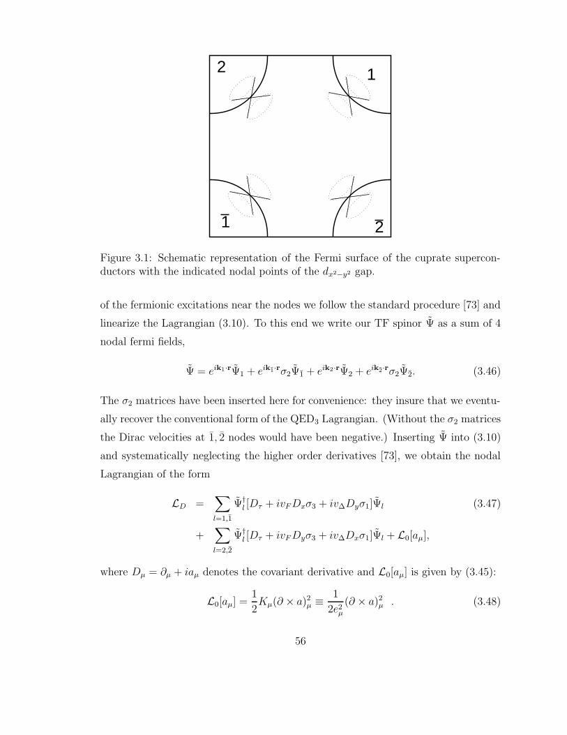
1 2
2 1
Figure 3.1: Schematic representation of the Fermi surface of the cuprate supercon-ductors with the indicated nodal points of the dx2−y2 gap.
of the fermionic excitations near the nodes we follow the standard procedure [73] and
linearize the Lagrangian (3.10). To this end we write our TF spinor Ψ as a sum of 4
nodal fermi fields,
Ψ = eik1·rΨ1 + eik1·rσ2Ψ1 + eik2·rΨ2 + eik2·rσ2Ψ2. (3.46)
The σ2 matrices have been inserted here for convenience: they insure that we eventu-
ally recover the conventional form of the QED3 Lagrangian. (Without the σ2 matrices
the Dirac velocities at 1, 2 nodes would have been negative.) Inserting Ψ into (3.10)
and systematically neglecting the higher order derivatives [73], we obtain the nodal
Lagrangian of the form
LD =∑
l=1,1
Ψ†l [Dτ + ivFDxσ3 + iv∆Dyσ1]Ψl (3.47)
+∑
l=2,2
Ψ†l [Dτ + ivFDyσ3 + iv∆Dxσ1]Ψl + L0[aµ],
where Dµ = ∂µ + iaµ denotes the covariant derivative and L0[aµ] is given by (3.45):
L0[aµ] =1
2Kµ(∂ × a)2
µ ≡ 1
2e2µ(∂ × a)2
µ . (3.48)
56
vF = ∂εk/∂k denotes the Fermi velocity at the node and v∆ = ∂∆k/∂k denotes the
gap velocity. Note that vF and v∆ already contain renormalizations coming from high
energy interactions and are effective material parameters of our theory. Similarly,
Kµ = 1/e2µ, derived in the previous Section in terms of ξsc(x, T ), are treated as
adjustable parameters which are matched to experimentally available information on
the range of superconducting correlations in the pseudogap state.
The massive Doppler gauge field vµ does not appear in the above expression, since
it merely generates short range interactions among the fermions.
In contrast, Berry gauge field aµ remains massless in the pseudogap state, as it
cannot acquire mass by coupling to the fermions. As seen from Eq. (3.47) aµ couples
minimally to the Dirac fermions and therefore its massless character is protected by
gauge invariance. Physically, one can also argue that aµ couples to the TF spin three-
current – in a spin-singlet d-wave superconductor SU(2) spin symmetry must remain
unbroken, thereby insuring that aµ remains massless. Its massless Maxwellian dy-
namics (3.48) in the pseudogap state can therefore be traced back to the topological
state of spacetime vortex loops and directly reflect the absence of true superconduct-
ing order or, equivalently, the presence of “vortex loop condensate” and dual order
(Appendix B.1).
We have also dispensed with the residual interactions represented by Hres in (3.2).
These interactions are generically short-ranged contributions from the p-h and am-
plitude fluctuations part of the p-p channel and in our new notation are exemplified
by:
Hres →1
2
∑
l,l′
Ill′Ψ†l ΨlΨ
†l′Ψl′ . (3.49)
The effective vertex Ill′ has a scaling dimension −1 at the engineering level. This
follows from the RG analysis near the massless Dirac points which sets the dimension
of Ψl to [length]−1. The implication is that Ill′ is irrelevant for low energy physics in
the perturbative RG sense and we are therefore justified in setting Ill′ → 0. However,
the residual interactions are known to become important if stronger than some critical
value Ic [74, 75]. In the present theory, this is bound to happen in the severely
underdoped regime and at half-filling, as x → 0 (see Section 3.6). In this case,
57
the residual interactions are becoming large and comparable in scale to the pairing
pseudogap ∆, and are likely to cause chiral symmetry breaking (CSB) which leads to
spontaneous mass generation for massless Dirac fermions. The CSB and its variety of
patterns in the context of the theory (3.47,3.48) in underdoped cuprates are discussed
in Section 3.6. Here, we shall focus on the chirally symmetric phase and assume
Ill′ < Ic, which we expect to be the case for moderate underdoping. Therefore, we
can set Ill′ → 0.
Finally, Eq. (3.47,3.48) represents the effective low energy theory for nodal TF.
This theory describes the problem of massless topological fermions interacting with
massless vortex “Beryons”, i.e. the quanta of the Berry gauge field aµ, and is formally
equivalent to the Euclidean quantum electrodynamics of massless Dirac fermions in
(2+1) dimensions (QED3). It, however, suffers from an intrinsic Dirac anisotropy by
virtue of vF 6= v∆.
3.3.1 Effective Lagrangian for the pseudogap state
Lagrangian (3.47) is not in the standard from as used in quantum electrodynamics
where the matrices associated with the components of covariant derivatives form
a Dirac algebra and mutually anticommute. In (3.47) the temporal derivative is
associated with unit matrix and it therefore commutes (rather than anticommutes)
with σ1 and σ3 matrices associated with the spatial derivatives. These nonstandard
commutation relations, however, lead to some rather unwieldy algebra. For this
reason we manipulate the Lagrangian (3.47) into a slightly different form that is
consistent with usual field-theoretic notation. First, we combine each pair of antipodal
(time reversed) two-component spinors into one 4-component spinor,
Υ1 =
(
Ψ1
Ψ1
)
, Υ2 =
(
Ψ2
Ψ2
)
. (3.50)
Second, we define a new adjoint four-component spinor
Υl = −iΥ†lγ0. (3.51)
58

In terms of this new spinor the Lagrangian becomes
LD =∑
l=1,2
ΥlγµD(l)µ Υl +
1
2Kµ(∂ × a)2
µ , (3.52)
with covariant derivatives
D(1)µ = i[(∂τ + iaτ ), vF (∂x + iax), v∆(∂y + iay)],
D(2)µ = i[(∂τ + iaτ ), vF (∂y + iay), v∆(∂x + iax)].
The 4 × 4 gamma matrices, defined as
γ0 =
(
σ2 0
0 −σ2
)
, γ1 =
(
σ1 0
0 −σ1
)
,
γ2 =
(
−σ3 0
0 σ3
)
(3.53)
now form the usual Dirac algebra,
γµ, γν = 2δµν (3.54)
and furthermore satisfy
Tr(γµ) = 0 , Tr(γµγν) = 4δµν . (3.55)
The use of the adjoint spinor Υ instead of conventional Υ† is a purely formal device
which will simplify calculations but does not alter the physical content of the theory.
At the end of the calculation we have to remember to undo the transformation (3.51)
by multiplying the 〈Υ(x)Υ(x′)〉 correlator by iγ0 to obtain the physical correlator
〈Υ(x)Υ†(x′)〉.Next, to make the formalism simpler still we can eliminate the asymmetry between
the two pairs of nodes by performing an internal SU(2) rotation at nodes 2, 2:
Υ2 → e−iπ4γ0γ1Υ2, (3.56)
leading to the anisotropic QED3 Lagrangian
LD =∑
l=1,2
Υlv(l)µ γµ(i∂µ − aµ)Υl +
1
2Kµ(∂ × a)2
µ , (3.57)
59
with v(1)µ = (1, vF , v∆) and v
(2)µ = (1, v∆, vF ).
We shall start by considering the isotropic case, vF = v∆ = 1, which although
unphysical in the strictest sense, is computationally much simpler and provides pen-
etrating insights into the physics embodied by the QED3 Lagrangian (3.57). After
we have understood the isotropic case we will then be ready to tackle the calcula-
tion for the general case and will show that Dirac cone anisotropy does not modify
the essential physics discussed here. To make contact with standard literature on
QED3, we further consider a more general problem with N pairs of nodes described
by Lagrangian
LD =
N∑
l=1
Υlγµ(i∂µ − aµ)Υl +1
2Kµ(∂ × a)2
µ . (3.58)
For the basic problem of a single CuO2 layer N = 2. As we will show in the next
Section, N itself is variable and can be equal to four or six in bi- and multi-layer
cuprates. Our analytic results can be viewed as arising from the formal 1/N expan-
sion, although we expect them to be qualitatively (and even quantitatively!) accurate
even for N = 2 as long as we are within the symmetric phase of QED3 – the quan-
titative accuracy stems from a fortuitous conspiracy of small numerical prefactors
[74].
3.3.2 Berryon propagator
Ultimately, we are interested in the properties of physical electrons. To describe
those we need to understand the properties of the electron–electron interaction medi-
ated by the gauge field aµ. To this end we proceed to calculate the Berry gauge field
propagator by integrating out the fermion degrees of freedom from the Lagrangian
(3.58). To one loop order this corresponds to evaluating the vacuum polarization
bubble Fig. 3.2(a). Employing the standard rules for Feynman diagrams in the
momentum space [76] the vacuum polarization reads:
Πµν(q) = N
∫
d3k
(2π)3Tr[G0(k)γµG0(k + q)γν]. (3.59)
Here G0(k) = kαγα/k2 is the free Dirac Green function, k = (k0,k) denotes the
Euclidean three-momentum, and the trace is performed over the γ matrices.
60

Figure 3.2: One loop Berryon polarization (a) and TF self energy (b).
The integral in Eq. (3.59) is a standard one (see Appendix B.2 for the details of
computation) and the result is
Πµν(q) =N
8|q|(
δµν −qµqνq2
)
, (3.60)
where |q| =√
q2. The one loop effective action for the Berry gauge field therefore
becomes (2π)−3∫
d3qLB with
LB[a] =
(
N
8|q| + 1
2e2q2
)(
δµν −qµqνq2
)
aµ(q)aν(−q) . (3.61)
At low energies and long wavelengths, |q|e2 N/4, the fermion polarization com-
pletely overwhelms the original Maxwell bare action term and the Berryon properties
become universal. In particular, the coupling constant 1/e2 drops out at low energies
and only reappears as the ultraviolet cutoff. Physically, the medium of massless Dirac
fermions screens the long range interactions mediated by aµ. In QED3 this screening
61

is incomplete: the gauge field becomes stiffer by one power of q but still remains
massless, in accordance with our general expectations. This anomalous stiffness of
aµ justifies the quadratic level expansion of L0 (3.45) and renders higher order terms
irrelevant in the RG sense. The theory therefore clears an important self-consistency
check.
At low energies the fully dressed Berryon propagator is given as an inverse of the
polarization,
Dµν(q) = Π−1µν (q) . (3.62)
In order to perform this inversion we have to fix the gauge. To this end we implement
the usual gauge fixing procedure by replacing qµqν/q2 → (1 − ξ−1)qµqν/q
2 in Eq.
(3.60). ξ ≥ 0 parameterizes the orbit of all covariant gauges. For example, ξ = 0
corresponds to Lorentz gauge kµaµ(k) = 0 while ξ = 1 corresponds to Feynman gauge.
Upon inversion we obtain the low energy Berryon propagator
Dµν(q) =8
|q|N
(
δµν −qµqνq2
(1 − ξ)
)
, (3.63)
in agreement with previous authors [81].
3.3.3 TF self energy and propagator
Topological fermion (TF) propagator is a gauge dependent entity and one could
therefore immediately object that as such it has no direct physical content and is of no
interest. While in the strictest sense, all observable quantities are gauge independent
and the 2−point fermion function is manifestly not gauge independent, the depen-
dence on the choice of gauge can be confined to the field strength renormalization
[82]. In this Section we will show that in the leading order in large N expansion,
the TF propagator is a powerlaw. The powerlaw exponent depends on the choice of
gauge. Since we know that the theory flows to the strong coupling limit, we expect
that the powerlaw exponent describing the physical spectrum is not trivial i.e. the
poles in the spectrum are replaced by a branchcut. This means that the plane wave
states acquire finite lifetime at arbitrarily low energy.
62

The lowest order (O(1/N)) self-energy diagram is depicted in Fig. 3.2(b) and reads
Σ(k) =
∫
d3q
(2π)3Dµν(q)γµG0(k + q)γν. (3.64)
Again, the computation is rather straightforward (see Appendix B.2 for details) and
the most divergent part is
Σ(k) =4(2 − 3ξ)
3π2N6k ln
(
Λ
|k|
)
, (3.65)
where we have introduced the Feynman “slash” notation, 6k = kµγµ.
To the leading 1/N order, the inverse TF propagator is given by
G−1(k) =6k[
1 + η ln
(
Λ
|k|
)]
(3.66)
with
η = −4(2 − 3ξ)
3π2N. (3.67)
Higher order contributions in 1/N will necessarily affect this result. Renormalization
group arguments [78] and non-perturbative approaches [79] strongly suggest that Eq.
(3.66) represents the start of a perturbative series that eventually resums into a power
law:
G−1(k) =6k(
Λ
|k|
)η
. (3.68)
This implies real-space propagator of the form
G(r) = Λ−η 6rr3+η
. (3.69)
Thus, the TF propagator exhibits a Luttinger-like algebraic singularity at small mo-
menta, characterized by an anomalous exponent η. In the Lorentz gauge (ξ = 0)
we find η = −8/3π2N ' −0.13, for N = 2. This rather small numerical value for
the anomalous dimension exponent (which is even considerably smaller for N = 4
or N = 6) indicates that the unraveling of the Fermi liquid pole in the original TF
propagator brought about by its interaction with the massless Berry gauge field is in
a certain sense “weak”. Note also that η is negative in the Lorentz gauge while it
becomes positive, η = 4/3π2N ' 0.06 for N = 2, in the Feynman gauge (ξ = 1). The
above results provide a strong indication that the physical, gauge-invariant fermion
propagator also has a Luttinger-like form, characterized by a small and positive anom-
alous dimension [58].
63
3.4 Effects of Dirac anisotropy in symmetric QED3
It is natural to examine to what extend is the theory modified by the inclusion of
the Dirac anisotropy, i.e. the finite difference in the Fermi velocity vF and the gap
velocity v∆. In the actual materials the Dirac anisotropy αD = vF
v∆decreases with
decreasing doping from ∼ 15 in the optimally doped to ∼ 3 in the heavily underdoped
samples.
There are two key issues: first, for a large enough number of Dirac fermion species
N , how is the chirally symmetric infrared (IR) fixed point modified by the fact that
αD 6= 1, and second, as we decrease N , does the chiral symmetry breaking occur at
the same value of N as in the isotropic theory. In this Section we address in detail
the first issue and defer the analysis of the second one to the future.
We determine the effect of the Dirac anisotropy, marginal by power counting, by
the perturbative renormalization group (RG) to first order in the large N expansion.
To the leading order δ in the small anisotropy αD = 1 + δ, we obtain the analytic
value of the RG βαD-function and find that it is proportional to δ, i.e. in the infra red
the αD decreases when δ > 0 and the anisotropic theory flows to the isotropic fixed
point. On the other hand, when δ < 0, αD increases in the IR and again the theory
flows into the isotropic fixed point. These results hold even when anisotropy is not
small as shown by numerical evaluation of the β-function. Upon integration of the RG
equations we find small δ acquires an anomalous dimension ηδ = 32/5π2N . Therefore,
we conclude that the isotropic fixed point is stable against small anisotropy.
Furthermore, we show that in any covariant gauge renormalization of Σ due to the
unphysical longitudinal degrees of freedom is exactly the same along any space-time
direction. Therefore the only contribution to the RG flow of anisotropy comes from
the physical degrees of freedom and our results for βαDstated above are in fact gauge
invariant.
64

3.4.1 Anisotropic QED3
In the realm of condensed matter physics there is no Lorentz symmetry to safe-
guard the space-time isotropy of the theory. Rather, the intrinsic Dirac anisotropy
is always present since it ultimately arises from complicated microscopic interactions
in the solid which eventually renormalize to band and pairing amplitude dispersion.
Thus there is nothing to protect the difference in the Fermi velocity vF = ∂εk∂k
and the
gap velocity v∆ = ∂∆k
∂kfrom vanishing and, in fact, all HTS materials are anisotropic.
The value of αD can be directly measured by the angle resolved photo-emission
spectroscopy (ARPES), which is ultimately a ”high” energy local probe of vF and
v∆. Since QED3 is free on short distances, we can take the experimental values as
the starting bare parameters of the field theory.
The pairing amplitude of the HTS cuprates has dx2−y2 symmetry, and consequently
there are four nodal points on the Fermi surface with Dirac dispersion around which
we can linearize the theory. Note that the roles of x and y directions are interchanged
between adjacent nodes. As before, we combine the four two-component Dirac spinors
for the opposite (time reversed) nodes into two four-components spinors and label
them as (1, 1) and (2, 2) (see Fig. 3.1).
Thus, the two-point vertex function of the non-interacting theory for, say, 11
fermions is
Γ(2)free
11= γ0k0 + vFγ1k1 + v∆γ2k2. (3.70)
Therefore the corresponding non-interacting “nodal” Green functions are
Gn0 (k) =
√gnµνγµkν
kµgµνkν≡ γnµkµ
kµgµνkν. (3.71)
Here we introduced the (diagonal) “nodal” metric g(n)µν : g
(1)00 =g
(2)00 =1, g
(1)11 =g
(2)22 =v2
F ,
g(1)22 =g
(2)11 =v2
∆, as well as the “nodal” γ matrices γn. In what follows we assume that
both vF and v∆ are dimensionless and that eventually one of them can be chosen to
be unity by an appropriate choice of the ”speed of light”.
Since αD 6= 1 breaks Lorentz invariance of the theory and since it is the Lorentz
invariance that protects the spacetime isotropy, we expect the β functions for αD to
acquire finite values. However, the theory still respects time-reversal and parity and
65

for N large enough the system is in the chirally symmetric phase. These symmetries
force the fermion self-energy of the interacting theory to have the form
Σ11 = A(k11, k22) (γ0k0 + vF ζ1γ1k1 + v∆ζ2γ2k2) . (3.72)
where k11 ≡ kµg(1)µν kν and k22 ≡ kµg
(2)µν kν. The coefficients ζi are in general different
from unity. Furthermore, there is a discrete symmetry which relates flavors 1, 1 and
2, 2 and the x and y directions in such a way that
Σ22 = A(k22, k11) (γ0k0 + v∆ζ2γ1k1 + vF ζ1γ2k2) . (3.73)
In the computation of the fermion self-energy, this discrete symmetry allows us to
concentrate on a particular pair of nodes without any loss of generality.
3.4.2 Gauge field propagator
As discussed above in the isotropic case, the effect of vortex-antivortex fluctuations
at T=0 on the fermions can, at large distances, be included by coupling the nodal
fermions minimally to a fluctuating U(1) gauge field with a standard Maxwell action.
Upon integrating out the fermions, the gauge field acquires a stiffness proportional to
k, which is another way of saying that at the charged, chirally symmetric fixed point
the gauge field has an anomalous dimension ηA = 1 (for discussion of this point in
the bosonic QED see [80]).
We first proceed in the transverse gauge (kµaµ = 0) which is in some sense the
most physical one considering that the ∇×a is physically related to the vorticity, i.e.
an intrinsically transverse quantity. We later extend our results to a general covariant
gauge. To one-loop order the screening effects of the fermions on the gauge field are
given by the polarization function
Πµν(k) =N
2
∑
n=1,2
∫
d3q
(2π)3Tr[Gn
0(q)γnµG
n0 (q + k)γnν ] (3.74)
where the index n denotes the fermion “nodal” flavor. The above expression can be
evaluated straightforwardly by noting that it reduces to the isotropic Πµν(k) once
66
the integrals are properly rescaled [58]. The result can be conveniently presented by
taking advantage of the “nodal” metric gnµν as
Πµν(k) =∑
n
N
16vFv∆
√
kαgnαβkβ
(
gnµν −gnµρkρg
nνλkλ
kαgnαβkβ
)
. (3.75)
Note that this expression is explicitly transverse, kµΠµν(k) = Πµν(k)kν = 0, and sym-
metric in its space-time indices. It also properly reduces to the isotropic expression
when vF = v∆ = 1.
However, as opposed to the isotropic case, it is not quite as straightforward to
determine the gauge field propagator Dµν . For example, as it stands the polarization
matrix (3.75) is not invertible, which makes it necessary to introduce some gauge-
fixing conditions. In our case the direct inversion of the 3 × 3 matrix would obscure
the analysis and therefore, we choose to follow a more physical and notationally
transparent line of reasoning which eventually leads to the correct expression for the
gauge field propagator. Upon integrating out the fermions and expanding the effective
action to the one-loop order, we find that
Leff [aµ] = (Π(0)µν + Πµν)aµaν (3.76)
where the bare gauge field stiffness is
Π(0)µν =
1
2e2k2
(
δµν −kµkνk2
)
. (3.77)
At this point we introduce the dual field bµ which is related to aµ as
bµ = εµνλqνaλ. (3.78)
Physically, the bµ field represents vorticity and we integrate over all possible vorticity
configurations with the restriction that bµ is transverse. We note that
L[bµ] = χ0b20 + χ1b
21 + χ2b
22 (3.79)
where χµ’s are functions of kµ and upon a straightforward calculation they can be
found to read
χµ =1
2e2+
N
16vFv∆
∑
n=1,2
gnννgnλλ
√
kαgnαβkβ
, (3.80)
67
where µ 6= ν 6= λ ∈ 0, 1, 2. At low energies we can neglect the non-divergent bare
stiffness and thus set 1/e2 = 0 in the above expression.
The expression (3.79) is manifestly gauge invariant and has the merit of not only
being quadratic but also diagonal in the individual components of bµ. Thus, integra-
tion over the vorticity (even with the restriction of transverse bµ) is simple and we
can easily determine the bµ field correlation function
〈bµbν〉 =δµνχµ
− kµkνχµχν
(
∑
i
k2i
χi
)−1
. (3.81)
The repeated indices are not summed in the above expression. Note that, in addition
to being transverse, 〈bµbν〉 is also symmetric in its space time indices.
It is now quite simple to determine the correlation function for the aµ field and in
the transverse gauge we obtain
Dµν(q) = 〈aµaν〉 = εµijενklqiqkq4
〈bjbl〉. (3.82)
Using the transverse character of 〈bµbν〉 (which is independent of the gauge) the above
expression can be further reduced to
Dµν(q) =1
q2
((
δµν −qµqνq2
)
〈b2〉 − 〈bµbν〉)
. (3.83)
It can be easily checked that in the isotropic limit the expression (3.83) properly
reduces to the results obtained in a different way.
We can further extend this result to include a general gauge by writing
Dµν(q) =1
q2
((
δµν − (1 − ξ
2)qµqνq2
)
〈b2〉 − 〈bµbν〉)
. (3.84)
where ξ is our continuous parameterization of the gauge fixing. This expression can
be justified by the Fadeev-Popov type of procedure starting from the Lagrangian
L =
(
Πµν +1
ξ
2k2
〈b2〉kµkνk2
)
aµaν , (3.85)
where the stiffness for the unphysical modes was judiciously chosen to scale as k in
a particular combination of the physical scalars of the theory. Note that 〈b2〉 can be
68

determined without ever considering gauge fixing terms. In this way, the extension
of a transverse gauge ξ = 0 to a general covariant gauge is accomplished by a simple
substitution kµkν → (1 − ξ2)kµkν. The expression (3.84) is our final result for the
gauge field propagator in a covariant gauge.
3.4.3 TF self energy
As discussed above, Σ is not gauge invariant in that it has an explicit dependence
on the gauge fixing parameter. As we will show in this Section (and more generally in
the Appendix B.3), the renormalization of Σ by the unphysical longitudinal degrees
of freedom does not depend on the space-time direction: the term in Σ which is
proportional to γ0 is renormalized the same way by the gauge dependent part of the
action as the terms proportional to γ1 and γ2. Therefore, the only contribution to
the RG flow of αD comes from the physical degrees of freedom.
We denote the topological fermion self-energy at the node n by Σn(q). Hence, to
the leading order in large N expansion we have
Σn(q) =
∫
d3k
(2π)3γnµG
n0 (q − k)γnνDµν(k). (3.86)
or explicitly
Σn(q) =
∫
d3k
(2π)3γnµ
(q − k)λγnλ
(q − k)µgµν(q − k)νγnνDµν(k), (3.87)
where the gauge field propagatorDµν is already screened by the nodal fermions (3.84).
Using the fact that
γµγλγν = iεµλνγ5γ3 + δµλγν − δµνγλ + δλνγµ, (3.88)
where µ, ν, λ ∈ 0, 1, 2 and γ5 ≡ −iγ0γ1γ2γ3, we can easily see that
γnµγnλγ
nνDµν = (2gnλµγ
nν − γnλg
nµν)Dµν , (3.89)
where we used the symmetry of the gauge field propagator tensor Dµν. Thus,
Σn(q) =
∫
d3k
(2π)3
(q − k)λ(2gnλµγ
nν − γnλg
nµν)Dµν(k)
(q − k)µgnµν(q − k)ν(3.90)
69

and as shown in the Appendix B.3 at low energies this can be written as
Σn(q) = −∑
µ
ηnµ(γnµqµ) ln
(
Λ√
qαgnαβqβ
)
. (3.91)
Here Λ is an upper cutoff and the coefficients η are functions of the bare anisotropy,
which have been reduced to a quadrature (see Appendix B.3). It is straightforward,
even if somewhat tedious, to show that in case of weak anisotropy (vF = 1+δ, v∆ = 1),
to order δ2,
η110 = − 8
3π2N
(
1 − 3
2ξ − 1
35(40 − 7ξ) δ2
)
(3.92)
η111 = − 8
3π2N
(
1 − 3
2ξ +
6
5δ − 1
35(43 − 7ξ) δ2
)
(3.93)
η112 = − 8
3π2N
(
1 − 3
2ξ − 6
5δ − 1
35(1 − 7ξ) δ2
)
. (3.94)
In the isotropic limit (vF = v∆ = 1) we regain ηnµ = −8(1 − 32ξ)/3π2N as previously
found by others.
3.4.4 Dirac anisotropy and its β function
Before plunging into any formal analysis, we wish to discuss some immediate
observations regarding the RG flow of the anisotropy. Examining the Eq. (3.91) it is
clear that if ηn1 = ηn2 then the anisotropy does not flow and remains equal to its bare
value. That would mean that anisotropy is marginal and the theory flows into the
anisotropic fixed point. In fact, such a theory would have a critical line of αD. For
this to happen, however, there would have to be a symmetry which would protect the
equality ηn1 = ηn2 . For example, in the isotropic QED3 the symmetry which protects
the equality of η’s is the Lorentz invariance. In the case at hand, this symmetry is
broken and therefore we expect that ηn1 will be different from ηn2 , suggesting that the
anisotropy flows away from its bare value. If we start with αD > 1 and find that
η112 > η11
1 at some scale p < Λ, we would conclude that the anisotropy is marginally
irrelevant and decreases towards 1. On the other hand if η112 < η11
1 , then anisotropy
continues increasing beyond its bare value and the theory flows into a critical point
with (in)finite anisotropy.
70
The issue is further complicated by the fact that ηnµ is not a gauge invariant
quantity, i.e. it depends on the gauge fixing parameter ξ. The statement that, say
ηn1 > ηn2 , makes sense only if the ξ dependence of ηn1 and ηn2 is exactly the same,
otherwise we could choose a gauge in which the difference ηn2 − ηn1 can have either
sign. However, we see from the equations (3.92-3.94) that in fact the ξ dependence
of all η’s is indeed the same. Although it was explicitly demonstrated only to the
O(δ2), in the Appendix B.3 we show that it is in fact true to all orders of anisotropy
for any choice of covariant gauge fixing. This fact provides the justification for our
procedure. Now we supply the formal analysis reflecting the above discussion.
The renormalized 2-point vertex function is related to the “bare” 2-point vertex
function via a fermion field rescaling Zψ as
Γ(2)R = ZψΓ(2). (3.95)
It is natural to demand that for example at nodes 1 and 1 at some renormalization
scale p, Γ(2)R (p) will have the form
Γ(2)R (p) = γ0p0 + vRF γ1p1 + vR∆γ2p2. (3.96)
Thus, the equation (3.96) corresponds to our renormalization condition through which
we can eliminate the cutoff dependence and calculate the RG flows.
To the order of 1/N we can write
Γ(2)R (p) = Zψγ
nµpµ
(
1 + ηnµ lnΛ
p
)
(3.97)
where we used the fermionic self-energy (3.91). Multiplying both sides by γ0 and
tracing the resulting expression determines the field strength renormalization
Zψ =1
1 + ηn0 ln Λp
≈ 1 − ηn0 lnΛ
p. (3.98)
We can now determine the renormalized Fermi and gap velocities
vRFvF
≈ (1 − η110 ln
Λ
p)(1 + η11
1 lnΛ
p) ≈ 1 − (η11
0 − η111 ) ln
Λ
p(3.99)
andvR∆v∆
≈ (1 − η110 ln
Λ
p)(1 + η11
2 lnΛ
p) ≈ 1 − (η11
0 − η112 ) ln
Λ
p. (3.100)
71

The corresponding renormalized Dirac anisotropy is therefore
αRD ≡ vRFvR∆
≈ αD(1 − (η112 − η11
1 ) lnΛ
p). (3.101)
The RG beta function can now be determined
βαD=
dαRDd ln p
= αD(η112 − η11
1 ). (3.102)
In the case of weak anisotropy (vF = 1 + δ, v∆ = 1) the above expression can be
determined analytically as an expansion in δ. Using Eqs.(3.93-3.94) we obtain
βαD=
8
3π2N
(
6
5δ(1 + δ)(2 − δ) + O(δ3)
)
. (3.103)
Note that this expression is independent of the gauge fixing parameter ξ. For 0 <
δ 1 the β function is positive which means that anisotropy decreases in the IR
and thus the anisotropic QED3 scales to an isotropic QED3. For −1 δ < 0 the β
function is negative and in this case the anisotropy increases towards the fixed point
αD = 1, i.e. again towards the isotropic QED3. Note that for δ > 2, β < 0 which may
naively indicate that there is a fixed point at δ = 2; this however cannot be trusted
as it is outside of the range of validity of the power expansion of ηµ. The numerical
evaluation of the β-function shows that, apart from the isotropic fixed point and the
unstable fixed point at αD = 0, βαDdoes not vanish (see Fig. 3.3). This indicates
that to the leading order in the 1/N expansion, the theory flows into the isotropic
fixed point where αD − 1 has a scaling dimension ηδ = 32/(5π2N) > 1.
3.5 Finite temperature extensions of QED3
In this Section we focus on thermodynamics and spin response of the pseudogap
state. First, in order to derive thermodynamics and spin susceptibility from the
QED3 theory [58] we generalize its form to finite T . This is a matter of some subtlety
since, the moment T 6= 0, the theory loses its fictitious “relativistic invariance”.
Second, we show that the theory predicts a finite T scaling form for thermodynamic
quantities in the pseudogap state. Third, we explicitly compute the leading T 6= 0
72

0 1 2 3 4 5αD
−2
0
2
4
6
8
10
12
β α D[8
/3π2 Ν
]
Figure 3.3: The RG β-function for the Dirac anisotropy in units of 8/3π2N . Thesolid line is the numerical integration of the quadrature in the Eq. (B.52) while thedash-dotted line is the analytical expansion around the small anisotropy (see Eq.(3.92-3.94)). At αD = 1, βαD
crosses zero with positive slope, and therefore at largelength-scales the anisotropic QED3 scales to an isotropic theory.
scaling and demonstrate that the deviations from “relativistic invariance” are actually
irrelevant for T much less than the pseudogap temperature T ∗, in the sense that the
leading order T 6= 0 scaling of thermodynamic functions remains that of the finite-T
symmetric QED3. These deviations from “relativistic invariance” do, however, affect
higher order terms. We illustrate these general results by computing the leading
(∼ T 2) and next-to-the leading (∼ T 3) terms in specific heat cv. Finally, we evaluate
magnetic spin susceptibility χu and show that it is bounded by T 2 at low T but
crosses over to ∼ T at higher T , closer to T ∗. Consequently, the Wilson ratio χuT/cv
vanishes as T → 0 implying the non-Fermi liquid nature of the pseudogap state in
cuprates.
We start by noting that the spin susceptibility of a BCS-like d-wave superconduc-
tor vanishes linearly with temperature. The way to understand this result is to notice
that the spin part of the ground state wavefunction, being a spin singlet, remains un-
perturbed by the application of a weak uniform magnetic field. However, the excited
quasiparticle states are not in general spin singlets and therefore contribute to the
thermal average of the spin susceptibility. Because their density of states is linear at
low energies, at finite temperature the number of quasiparticles that are excited is
∼ kBT , each contributing a constant to the Pauli-like uniform spin susceptibility χu.
Thus χu ∼ T .
73

When the superconducting order is destroyed by proliferation of unbound quantum
hc/2e vortices, the low-energy quasiparticle excitations are strongly interacting. The
interaction originates from the fact that it is the spin singlet pairs that acquire a
one unit of angular momentum in their center of the mass coordinate, carried by
a hc/2e vortex. This translates into a topological frustration in the propagation
of the “spinon” excitations. As a result, non-trivial spin correlations persist in the
excited states of the phase-disordered d-wave superconductor. At low temperature,
this leads to a suppression of χu relative to that of the non-interacting quasiparticles.
We shall argue below that in the phase-disordered superconductor, χu ∼ T 2 at low
temperatures.
Similarly, in a d-wave superconductor, linear density of the quasiparticle states
translates into T 2 dependence of the low T specific heat. When the interactions
between quasiparticles are included the spectral weight is transferred to multi-particle
states. Within QED3 theory, however, the strongly interacting IR (infra-red) fixed
point possesses emergent “relavistivistic invariance” at long distances and low energies
and the dynamical critical exponent z = 1. Furthermore, the effective quantum action
for vortices, deep in the phase disordered pseudogap state, introduces an additional
lengthscale, the superconducting correlation length ξτ,⊥ (labels τ and ⊥ stand for
time- and space-like, respectively). At T = 0 this scale serves as a short distance
cutoff of the theory and possesses some degree of doping (x) dependence within the
pseudogap state. We then argue that under rather general circumstances the low T
electronic specific heat scales as T 2 while the free energy goes as T 3.
Deep in the phase disordered pseudogap state the fluctuations in the vorticity
3-vector bµ = εµνλ∂νaλ are described by the “bare” Lagrangian of the QED3 theory
[58]:
L0(aµ) =K⊥2f⊥
(
T
k,T
ω, TK⊥,τ
)
b20 +Kτ
2fτ
(
T
k,T
ω, TK⊥,τ
)
~b2, (3.104)
where fτ (0, 0, 0) = f⊥(0, 0, 0) = 1. fτ,⊥ are general scaling functions describing how
L0(aµ) is modified from its “relativistically invariant” T = 0 form as the temperature
is turned on, and K⊥,τ is related to the superconducting correlation length as Kτ ∝ξ2sc/ξτ and K⊥ ∝ ξτ [58]. Physically, such modifications are due to changes in the
74
pattern of vortex-antivortex fluctuations induced by finite T .
To handle the intrinsic space-time anisotropy, it is convenient to introduce two
tensors
Aµν =
(
δµ0 −kµk0
k2
)
k2
~k2
(
δ0ν −k0kνk2
)
,
Bµν = δµi
(
δij −kikj~k2
)
δjν , (3.105)
and rewrite the gauge field action as
L0(aµ) =1
2Π0AaµAµνaν +
1
2Π0BaµBµνaν . (3.106)
For details see Appendix B.4. It is straightforward to show that
Π0A = Kτfτ
(
T
k,T
ω, TK⊥,τ
)
(~k2 + ω2),
Π0B = Kτfτ
(
T
k,T
ω, TK⊥,τ
)
ω2 +K⊥f⊥
(
T
k,T
ω, TK⊥,τ
)
~k2.
(3.107)
The gauge field aµ couples minimally to the Dirac fermions representing nodal
BCS quasiparticles [58]. Consequently, the resulting Lagrangian reads
L = ψ (iγµ∂µ + γµaµ)ψ + L0(aµ) . (3.108)
The integration over Berry gauge field aµ reproduces the interaction among quasipar-
ticles arising from the topological frustration referred to earlier.
3.5.1 Specific heat and scaling of thermodynamics
The only lengthscales that appear in the thermodynamics are the thermal length ∼1/T , and the superconducting correlation lengths K⊥,τ . At T = 0, the two correlation
lengths enter only as short distance cutoffs for the theory since the electronic action
is controlled by the IR fixed point of QED3. These observations allow us to write
down the general scaling form for the free energy
F(T ; x) = T 3Φ(
Kτ (x)T,K⊥(x)T)
. (3.109)
75
In the above scaling form K⊥ is related to the T → 0 finite superconducting correla-
tion length of the pseudogap state ξsc(x). The ratio Kτ/Ksc describes the anisotropy
between time-like and space-like vortex fluctuations and is also a function of doping
x. The scaling expressions for other thermodynamic functions can be derived from
(3.109) by taking appropriate temperature derivatives. For details see Appendices
B.5 and B.6.
We are interested in the limit of the thermal length 1/T being much longer than
Kτ and K⊥ i.e. in the limit of Φ(x → 0, y → 0). This is precisely the limit in which
the free energy approaches the free energy of the finite temperature QED3. Therefore,
Φ(x, y) is regular at x = y = 0 (see Ref.[81]) and so in the limit of T → 0, F ∼ T 3 or
cv ∼ T 2.
3.5.2 Uniform spin susceptibility
The fermion fields ψ were defined in Ref. [58] where it is shown that the physical
spin density ψ†↑ψ↑ − ψ†
↓ψ↓ is equal to the Dirac fermion density ψγ0ψ.
To compute the spin-spin correlation function 〈Sz(−k)Sz(k)〉 we introduce an
auxiliary source Jµ(k) and couple it to fermion three current. Thus
L[ψ, ψ, aµ, Jµ] = ψ (iγµ∂µ + γµ(aµ + Jµ))ψ + L0(aµ) (3.110)
and since it is the z-component of the spin that couples to the gauge field we have
〈Sz(−k)Sz(k)〉 =1
Z[Jµ]
δ
δJ0(−k)δ
δJ0(k)Z[Jµ]
∣
∣
∣
Jµ=0, (3.111)
Z being the quantum partition function. Now we let a′µ = aµ + Jµ and integrate
out both the fermions and the gauge field a′µ. The correlations between a′µ fields are
described by the polarization matrix which to the order of 1/N can be written in the
form Πµν = (Π0A + ΠF
A)Aµν + (Π0B + ΠF
B)Bµν. The resulting spin correlation function
is then readily found to be
〈Sz(−k)Sz(k)〉 =ΠFAΠ0
A
ΠFA + Π0
A
~k2
~k2 + ω2, (3.112)
76
where ΠFA denotes the fermion current polarization function. Due to the scale invari-
ance of the (massless) fermion action, the time component of the retarded polarization
function has the scaling form
ΠF retA (q, ω, T ) = NT PF
A
( q
T,ω
T
)
, (3.113)
where PFA (x, y) is a universal function of its arguments and N is the number of the
4−component fermion species (see Appendix B.5). In the static limit, ω → 0,
limy→0
Re PFA (x, y) =
2 ln 2
π+
x2
24π+ O(x3); x 1 (3.114)
and
limy→0
Re PFA (x, y) =
x
8+
6ζ(3)
πx2+ O(x−3); x 1 (3.115)
while
limy→0
Im PFA (x, y) =
2 ln 2
π
y
x+ O
(
y2
x2
)
; x 1 (3.116)
In addition, in the limit of ω = 0 and k → 0 we have
fτ
(
T
k,∞, KτT
)
→ 1 + cT 2
k2(3.117)
where c is a pure number. Combining all of these results together we have
χ(ω = 0, q → 0) =2N ln 2
π
KτT2
2N ln 2πc
+KτT. (3.118)
There are several sources of correction to the scaling, and it is impossible to address
all of them without an explicit model for the vortices. Instead, we will concentrate on
the particular case of the corrections to scaling due to the Dirac cone anisotropy. It
was shown in the previous Section that the Dirac cone anisotropy αD = vF/v∆ scales
to unity at the QED3 IR fixed point. Alternatively, when defined as αD ≡ 1 + δ, δ
has a scaling dimension ηδ > 1. To the leading order in 1/N , ηδ = 32/(5π2N) (see
the previous Section). For simplicity, we assume that the bare action for the gauge
field is e−2F 2µν . Then the T dependence of the free energy scales as
F =T 3
v2F
Φ
(
T
e2,vFv∆
)
=T 3
v2F
Φ
(
T
e2, 1 + δ(T )
)
(3.119)
77

Thus, in the limit of T → 0 we have
F =T 3
v2F
Φ (0, 1) +T 3+ηδ
v2F
δ0Φ′ (0, 1) . (3.120)
Therefore, while the leading order scaling of the free energy is analytic T 3, the cor-
rection to scaling is non-analytic T 3+ηδ .
3.6 Chiral symmetry breaking
In this Section we shall try to understand the physical nature of the instabilities
of the symmetric phase of QED3 or Algebraic Fermi Liquid.
We show that a phase disordered d-wave superconductor, as introduced in pre-
vious sections, becomes an antiferromagnet [83]. The antiferromagnetism emerges
via a phenomenon of spontaneous chiral symmetry breaking (CSB)[59, 60]. Away
from half filling, the broken symmetry phase typically takes the form of an incom-
mensurate spin-density-wave (SDW), whose periodicity is tied to the Fermi surface.
Furthermore, we show that numerous other states, most notably a d+ip and a d+is
phase-incoherent superconductors (dipSC, disSC) and “stripes”, i.e. superpositions
of 1D charge-density-waves (CDW) and phase-incoherent superconducting-density-
waves (SCDW), as well as continuous chiral rotations among them, are all energeti-
cally close and competitive with antiferromagnetism due to their equal membership
in the chiral manifold of two-flavor (N = 2) QED3. This large chiral manifold of
nearly degenerate states plays the key role in the QED3 theory as the culprit behind
the complexity of the HTS phase diagram.
The above results place tight restrictions on this phase diagram and provide means
to unify the phenomenology of cuprates within a single, systematically calculable
“QED3 Unified Theory” (QUT). Any microscopic description of cuprates, as long
as it leads to the large d-wave pairing pseudogap with T ∗ Tc → 0, will conform
to the general results of QUT. In particular, all the physical states in natural ener-
getic proximity to a d-wave superconductor are the ones inhabiting the above chiral
manifold.
78
For the sake of concreteness we restate the starting Lagrangian 3.47
LQED = ψncµ,nγµDµψn + L0[aµ] + (· · · ). (3.121)
Here ψ†α = ψαγ0 = (η†α, η
†α) are the four-component Dirac spinors with η†α = 1√
2Ψ†α(1+
iσ1), η†α = 1√
2Ψ†ασ2(1 + iσ1), and Ψ†
α = (ψ†↑α, ψ↓α). Fermion fields ψσα(r, τ) describe
‘topological fermions’ of the theory and are related to the original nodal fermions
cσα(r, τ) via the singular gauge transformation (3.4). Index n labels (1, 1) and (2, 2)
pairs of nodes while α labels individual nodes, µ = τ, x, y(≡ 0, 1, 2). Dµ = ∂µ + iaµ
is a covariant derivative, cτ,n = 1, cx,1 = cy,2 = vF , cx,2 = cy,1 = v∆. The gamma
matrices are defined as γ0 = σ3 ⊗ σ3, γ1 = −σ3 ⊗ σ1, γ2 = −σ3 ⊗ σ2, and satisfy
γµ, γν = 2δµν . The Berry gauge field aµ encodes the topological frustration of
nodal fermions generated by fluctuating quantum vortex-antivortex pairs and L0 is
its bare action. The loss of superconducting phase coherence caused by unbinding of
vortex pairs is heralded in (3.121) by aµ becoming massless:
L0 →1
2e2τ(∂ × a)2
τ +∑
i
1
2e2i(∂ × a)2
i ; (3.122)
here e2τ , e
2i (i = x, y), as well as the velocities vF (∆), are functions of doping x and T .
Along with residual interactions between nodal fermions, denoted by the ellipsis in
(3.121), these parameters of QUT arise from some more microscopic description and
will be discussed shortly.
LQED (3.121) possesses the following peculiar continuous symmetry: borrowing
from ordinary quantum electrodynamics in (3+1) dimensions (QED4), we know that
there exist two additional gamma matrices, γ3 = σ1 ⊗ 1 and γ5 = iσ2 ⊗ 1 that anti-
commute with all γµ. We can define a global U(2) symmetry for each pair of nodes,
with generators 1 ⊗ 1, γ3, −iγ5 and 12[γ3, γ5], which leaves LQED invariant. In QED3
this symmetry can be broken by two “mass” terms, mchψnψn and mPTψn12[γ3, γ5]ψn.
Spontaneous symmetry breaking in QED3 as a mechanism for dynamical mass gen-
eration has been extensively studied in the field theory literature [59]. It has been
established that while mPT is never spontaneously generated [84], the chiral mass mch
is generated if number of fermion species N is less than a critical value Nc. While
79

dSC
dSC
CSB
CSB
a
b
3QED
SDW/AF dSC
x(CSB)
T
T*
Tc
Figure 3.4: Schematic phase diagram of a cuprate superconductor in QUT. Dependingon the value of Nc (see text), either the superconductor is followed by a symmetric
phase of QED3 which then undergoes a quantum CSB transition at some lower doping(panel a), or there is a direct transition from the superconducting phase to the mch 6=0 phase of QED3 (panel b). The label SDW/AF indicates the dominance of theantiferromagnetic ground state as x→ 0.
still a matter of some controversy, standard non-perturbative methods give Nc ∼ 3
for isotropic QED3[59, 60], but as we shall discuss shortly, anisotropy and irrelevant
couplings present in Lagrangian (3.121) can change the value of Nc.
Let us now assume that CSB occurs and the mass term mchψnψn is generated. We
wish to determine what is the nature of this chiral instability in terms of the original
electron operators. To make this apparent, let us consider a general chiral rotation
ψn → U(n)ch ψn with U
(n)ch = exp(iθ3nγ3 + θ5nγ5). Within our representation of Dirac
spinors (3.121), the mchψnψn mass term takes the following form:
mch cos(2Ωn)[
η†ασ3ηα − η†ασ3ηα]
+
+mch sin(2Ωn)θ5n + iθ3n
Ωnη†ασ3ηα + h.c. , (3.123)
where Ωn =√
θ23n + θ2
5n. mch acts as an order parameter for the bilinear combinations
of topological fermions appearing in (3.123). In the symmetric phase of QED3 (mch =
80

1 2
22Q Q
11
2 1
Q12
Figure 3.5: The “Fermi surface” of cuprates, with the positions of nodes in the d-wavepseudogap. The wavectors Q11,Q22,Q12, etc. are discussed in the text.
0) the expectation values of such bilinears vanish, while they become finite, 〈ψnψn〉 6=0, in the broken symmetry phase.
The chiral manifold (3.123) is spanned by the “basis” of three symmetry breaking
states. When re-expressed in terms of the original nodal fermions cσα(r, τ), two of
these involve pairing in the particle-hole (p-h) channel – a cosine and a sine spin-
density-wave (SDW):
〈c†↑αc↑α − c†↓αc↓α〉 + h.c. (cos SDW)
i〈c†↑αc↑α − c†↑αc↑α〉 + (↑→↓) (sin SDW) (3.124)
and are obtained from Eq. (3.123) by setting Ωn equal to π/4 or 3π/4. Rotations
within the chiral manifold (3.123) at fixed Ωn correspond to the sliding modes of
SDW.
A simple physical picture emerges here: we started from a d-wave superconducting
phase, our parent state. As one moves closer to half-filling and true phase coherence
is lost, strong vortex-antivortex pair fluctuations, acting under the protective um-
brella of a d-wave particle-particle (p-p) pseudogap, spontaneously induce formation
of particle-hole “pairs” at finite wavevectors ±Q11 and ±Q22, spanning the Fermi
81

surface from node α to α (Fig. 3.5). The glue that binds these p-h “pairs” and plays
the role of “phonons” in this pairing analogy is provided by the Berry gauge field aµ.
Such “fermion duality” is a natural consequence of the QED3 theory (3.121). Remark-
ably, we find the antiferromagnetic insulator being spontaneously generated in form
of the incommensurate SDW. As we get very near half-filling and Q11,Q22 approach
(±π,±π), SDW acquires the most favored state status within the chiral manifold –
this is the consequence of umklapp processes which increase its condensation energy
without it being offset by either the anisotropy or a poorly screened Coulomb interac-
tion which plagues its CDW competitors to be introduced shortly. It seems therefore
reasonable to argue that this SDW must be considered the progenitor of the Neel-
Mott-Hubbard insulating antiferromagnet at half-filling. Thus, QED3 theory (3.121)
explains the origin of antiferromagnetic order in terms of strong vortex-antivortex
fluctuations in the parent d-wave superconductor. It does so naturally, through its
inherent and well-established chiral symmetry breaking instability [59].
The chiral manifold (3.123) contains also a third state, a p-p pairing state cor-
responding to Ωn = 0 or π/2 and best characterized as a d+ip phase-incoherent
superconductor:
i〈ψ↑αψ↓α − ψ↑αψ↓α〉 + h.c. (dipSC) . (3.125)
We have written dipSC in terms of topological fermions ψσα(r, τ) since use of the
original fermions leads to more complicated expression which involves the backflow of
vortex-antivortex excitations described by gauge fields aµ and vµ (such backflow terms
do not arise in the p-h channel). This state breaks parity but preserves time reversal,
translational invariance and superconducting U(1) symmetries. To our knowledge,
such state has not been proposed as a part of any of the major theories of HTS. It is
an intriguing question whether this d+ip phase-incoherent superconductor can be the
actual ground state at some dopings in some of the cuprates. Its energetics does not
suffer from long range Coulomb problems but it is clearly inferior to the SDW very
close to half-filling since, being spatially uniform, it receives no help from umklapp.
Until now, we have discussed the CSB pattern only within individual pairs of
nodes, (1,1) and (2,2). What happens if we allow for chiral rotations that mix nodes
82

1 and 2 or 1 and 2? A whole new plethora of states becomes possible, with chiral
manifold enlarged to include a superposition of one-dimensional p-h and p-p states,
an incommensurate CDW accompanied by a non-uniform phase-incoherent supercon-
ductor (SCDW) at wavevectors ±Q12 and ±Q21 (Fig. 3.5):
1√2〈c†↑1c↑2 + c†↑2c↑1 + h.c.〉 + (↑→↓) (CDW)
1√2〈ψ↑1ψ↓2 + ψ↑2ψ↓1 + h.c.〉 + (↑↔↓) (SCDW) (3.126)
These same states, rotated by π/2, are replicated at wavevectors ±Q12 and ±Q21
(Fig. 2). In a fluctuating dx2−y2 superconductor these CDWs and SCDWs run along
the x and y axes and are naturally identified as the “stripes” of QUT. Note, however,
these are not the only one-dimensional states in QUT – among the states in the chiral
manifold (3.123) are also “diagonal stripes”, the combination of a SDW (3.124) along
±Q11 and a dipSC (3.125) which opens the mass gap only at nodes (2, 2), or vice
versa. Furthermore, a phase-incoherent d+is superconductor (disSC) is also present
within the chiral enlarged manifold, since it results in alternating signs for different
nodes with equal number of positive and negative “masses” for the two-component
nodal fermions:
i〈ψ↑1ψ↓1 + ψ↑1ψ↓1 + h.c.〉 + (1 → 2) (disSC) . (3.127)
In contrast, in a d+id phase incoherent superconductor these “masses” have the
same sign for all the nodes producing a maximal breaking of the PT symmetry [84].
Consequently, a d+id phase-incoherent superconductor is not spontaneously induced
within the QED3 theory.
In the isotropic (vF = v∆) N = 2 QED3 all these additional states plus arbitrary
chiral rotations among them are completely equivalent to those discussed previously.
It is here where we confront the problem of intrinsic anisotropy in Eq. (3.121). Such
anisotropy cannot be rescaled out and manifestly breaks the U(2)×U(2) degeneracy
of the full N = 2 chiral manifold down to two separate U(1)×U(1) (3.123) chiral
groups discussed previously. This is reflected in the general increase in energy of
the states from the enlarged chiral manifold. For example, the anisotropy raises the
83

energy of our “stripe” states (3.126) relative to those of SDW, dipSC or “diagonal
stripes”. However, when the long range Coulomb interactions and coupling to the
lattice are included in the problem, as they are in real materials, it is conceivable
that the “stripes” would return in some form, either as a ground state or a long-lived
metastable state at some intermediate doping. disSC is also adversely affected by
anisotropy but to a lesser extent and might remain competitive with SDW, dipSC
and “diagonal stripes”. This state breaks time reversal symmetry but preserves parity
and the discussion concerning dipSC below Eq. (3.125) applies to disSC equally well.
How do we use these general results on CSB in QUT to address the specifics of
cuprate phase diagram? To this end, we need some effective combination of phenom-
enology and more microscopic descriptions to determine the parameters vF , v∆, eτ ,
ei and residual interactions (· · · ) appearing in LQED (3.121). The main task is to
determine what is the sequence of states within QUT that form stable phases as the
doping decreases toward half-filling under T ∗ in Fig. 3.4. While this is an extensive
project for the future, we outline here some of the general features. First, within
the superconducting state eτ , ei → 0 and aµ becomes massive thus denying the CSB
mechanism its main dynamical agent. We therefore expect that the superconductor
is in the symmetric phase and its nodal fermions form well-defined excitations[58].
As we move to the left in Fig. 3.4, the phase order is suppressed and eτ , ei become
finite, reflecting the unbinding of vortex-antivortex excitations[58]. For all practical
purposes, this is precisely what the experiments imply. Now, the key question is
whether the QED3 (3.121) remains in its symmetric phase or whether it immediately
undergoes the CSB transition and generates finite gap (mch 6= 0).
This question is difficult to answer in detail, because Nc can depend non-universally
on higher order coupling constants. For instance, short range interactions, while per-
turbatively irrelevant, effectively increase Nc if stronger than some critical value[74].
Such interactions, typically in the form of short range three-current terms[21], arise in
more microscopic models used to derive LQED and are prominent among the residual
terms denoted by ellipsis in (3.121). Their strength generically increases as x → 0.
These residual interactions play a dual role in QUT. First, they can conspire with the
anisotropy to produce the situation depicted in panel (b) of Fig. 3.4, where the CSB
84

takes place as soon as the phase coherence is lost. Second, once the chiral symmetry
has been broken, the residual interactions further break the symmetry within the
chiral manifold (3.123) and play a role in selecting the true ground state.
3.7 Summary and conclusions
We considered the effect of fluctuations in the d-wave superconductor, concen-
trating on the role of the phase fluctuations and their effect on the nodal fermions.
The pairing pseudogap provided a reference point of our analysis which allowed us to
classify various quasiparticle interactions according to their fate under the renormal-
ization group. By carefully treating the interactions of the quasiparticles with the
vortex phase defects, we find that the low energy effective theory for the quasiparti-
cles inside the pairing protectorate is the (2+1) dimensional quantum electrodynamics
(QED3) with inherent spatial anisotropy, described by Lagrangian LD specified by
Eqs. (3.47,3.57).
Within the superconducting state the gauge fields of the theory are massive by
virtue of vortex defects being bound into finite loops or vortex-antivortex pairs. Such
massive gauge fields produce only short ranged interactions between our BdG qua-
siparticles and are therefore irrelevant: in the superconductor quasiparticles remain
sharp in agreement with prevailing experimental data [85]. Loss of the long range
superconducting order is brought about by unbinding the topological defects – vor-
tex loops or vortex-antivortex pairs – via Kosterlitz-Thouless type transition and its
quantum analogue. Remarkably, this is accompanied by the Berry gauge field becom-
ing massless. Such massless gauge field mediates long range interactions between the
fermions and becomes a relevant perturbation. Exactly what is the consequence of
this relevant perturbation depends on the number of fermion species N in the prob-
lem. For cuprates we argued that N = 2nCuO where nCuO is the number of CuO2
layers per unit cell. If N < Nc ' 3 [59], the interactions cause spontaneous opening
of a gap for the fermionic excitations at T = 0, via the mechanism of chiral symmetry
breaking in QED3 [59]. Formation of the gap corresponds to the onset of AF SDW
instability [58, 83] which must be considered as a progenitor of the Mott-Hubbard-
85

Neel antiferromagnet at half-filling. If, on the other hand, N > Nc as will be the
case in bilayer or trilayer materials, the theory remains in its chirally symmetric non-
superconducting phase even as T → 0 and AF order arises from within such state
only upon further underdoping (Fig. 1). We call this symmetric state of QED3 an
algebraic Fermi liquid (AFL). In both cases AFL controls the low temperature, low
energy behavior of the pseudogap state and in this sense assumes the role played by
Fermi liquid theory in conventional metals and superconductors. In AFL the quasi-
particle pole is replaced by a branch cut – the quasiparticle is no longer sharp – and
the fermion propagator acquires a Luttinger-like form Eq. (3.68). To our knowledge
this is one of the very few cases where a non-Fermi liquid nature of the excitations
has been demonstrated in dimension greater than one in the absence of disorder or
magnetic field. This Luttinger-like behavior of AFL will manifest itself in anomalous
power law functional form of many physical properties of the system.
Dirac anisotropy, i.e. the fact that vF 6= v∆, plays important role in the cuprates
where the ratio αD = vF/v∆ in most materials ranges between 3 and 15−20. Such
anisotropy is nontrivial as it cannot be rescaled and it significantly complicates any
calculation within the theory. Using the perturbative renormalization group theory
we have shown that anisotropic QED3 flows back into isotropic stable fixed point.
This means that for weak anisotropy at long lengthscales the universal properties of
the theory are identical to those of the simple isotropic case. It remains to be seen
what are the properties of the theory at intermediate lengthscales when anisotropy is
strong.
The QED3 theory of the pairing pseudogap, as presented in here, starts from a
remarkably simple set of assumptions, and via manipulations that are controlled in
the sense of 1/N expansion, arrives at nontrivial consequences, including the algebraic
Fermi liquid and the antiferromagnet.
86
Appendix A
Quasiparticle correlation functions
in the mixed state
A.1 Green’s functions: definitions and identities
The one-particle Green’s function matrix [52] is defined as
Gαβ(r1τ1; r2τ2) ≡ −〈TτΨα(1)Ψ†β(2)〉 (A.1)
where Tτ denotes imaginary time ordering operator and α = 1, 2 denotes components
of a Nambu spinor Ψ†(1) which is a shorthand for Ψ†(r1, τ1) =(
ψ†↑(r1, τ1), ψ↓(r1, τ1)
)
.
Due to the time independence of the Hamiltonian (2.2), the Green’s function (A.1)
depends only on the imaginary time difference τ = τ1 − τ2. Therefore, its Fourier
transform is given by
G(r1, r2; iω) =∫ β
0eiωτ G(r1, r2, τ)dτ
G(r1, r2; τ) = 1β
∑
iω
e−iωτ G(r1, r2; iω).
(A.2)
Here β = 1/(kBT ), T is temperature, and the fermionic frequency ω = (2l + 1)π/β, l ∈ Z.
Using the above relations, it is straightforward to derive the spectral representation
of the following correlation functions between Ψ and its imaginary time derivatives
87
∂τΨ ≡ Ψ:
〈TτΨα(1)Ψ†β(2)〉
〈Tτ Ψα(1)Ψ†β(2)〉
〈TτΨα(1)Ψ†β(2)〉
〈Tτ Ψα(1)Ψ†β(2)〉
= − 1
β
∑
iω
e−iwτ∫
dεA(r1, r2; ε)
iω − ε
+1
−ε+ε
−ε2
(A.3)
The spectral function A(r1, r2; ε) can be written in terms of eigenfunctions Φn(r) =
(un(r), vn(r))T of the Bogoliubov-deGennes Hamiltonian H0 in the form:
Aαβ(r1, r2; ε) =∑
n
δ(ε− εn)Φnα(r1)Φ†nβ(r2), (A.4)
where εn is the eigen-energy associated with an eigenstate labeled by the quantum
number n. Substituting (A.4) into (A.3) we can write the above correlation functions
solely in terms of the eigenfunctions Φn(r):
〈TτΨα(1)Ψ†β(2)〉
〈Tτ Ψα(1)Ψ†β(2)〉
〈TτΨα(1)Ψ†β(2)〉
〈Tτ Ψα(1)Ψ†β(2)〉
=− 1
β
∑
iω,n
e−iwτΦnα(r1)Φ
†nβ(r2)
iω − εn
+1
−εn+εn
−ε2n
(A.5)
In the calculations that follow we will also encounter Matsubara summations over
the fermionic frequencies ω = (2l + 1)π/β, l ∈ Z, of the form:
Snm(iΩ) =1
β
∑
iω
1
(iω − εn)(iΩ + iω − εm)(A.6)
where Ω = 2πk/β, k ∈ Z, is an outside bosonic frequency. The sum (A.6) can be
evaluated using standard techniques (see e.g. [52]) and yields:
Snm(iΩ) =fn − fm
εn − εm + iΩ. (A.7)
Here fn is a short hand for the Fermi-Dirac distribution function f(εn) =(
1 +
exp(βεn))−1
.
In order to derive spin and thermal currents we will need the explicit form of the
generalized velocity operator V introduced in (2.33):
V =
(
π
miv∆
iv∗∆
π∗
m
)
(A.8)
88
where the gap velocity operator is given by
iv∆ = i∆0ηδδeiφ(r)/2
(
eiδ·p − e−iδ·p)
eiφ(r)/2 (A.9)
and the canonical momentum equals
π=− i
2δe
i~
r+δr
(p− ecA)·dl + h.c. (A.10)
The following identities for operators v∆ and π will be used in the next section:
π∗Ψ† · πΨ = i~∇ · (Ψ†πΨ) + Ψ†π2Ψ
π∗Ψ† · πΨ = −i~∇ · (π∗Ψ† Ψ) + (π∗)2Ψ† Ψ(A.11)
Ψ†∆Ψ − ∆Ψ† Ψ =1
2∇ ·(
Ψ† v∆Ψ − v∆Ψ† Ψ)
(A.12)
The above equations are straightforward to derive in continuum, while on the tight-
binding lattice Eqs. (A.11) and (A.12) imply a symmetric definition of the lattice
divergence operator.
The identities (A.11,A.12) explicitly ensure that the generalized velocity operator
Vµ is Hermitian i.e it satisfies the following identity:∫
drV∗Ψ†(r) Ψ(r) ≡∫
drV∗αβΨ
†β(r) Ψα(r)
=
∫
drΨ†(r) VΨ(r). (A.13)
A.2 Spin current and spin conductivity tensor
The time derivative of spin density ρs = ~
2(ψ†
↑ψ↑−ψ†↓ψ↓) can be written in Nambu
formalism as
ρs =i
~[H, ρs] =
~
2(Ψ†Ψ + Ψ†Ψ) (A.14)
Using equations of motion (2.10) together with the explicit form of H0 operator (2.8)
we obtain
ρs =i
2
(
(π∗)2
2m؆
1 Ψ1 − Ψ†1
π2
2mΨ1 + ∆Ψ†
1 Ψ2 − Ψ†1∆Ψ2
+ ∆∗Ψ†2 Ψ1 − Ψ†
2 ∆∗Ψ1 −π2
2m؆
2 Ψ2 + Ψ†2
(π∗)2
2mΨ2
)
. (A.15)
89
Using the identities (A.11,A.12) it is easy to show that
ρs = −~
4∇µ(Ψ
†VµΨ + V ∗µΨ† Ψ) = −∇ · js (A.16)
where the generalized velocity operator Vµ is defined in Eq. (A.8), and the last
equality follows from the continuity equation (2.31) relating the spin density ρs and
the spin current js. Upon spatial averaging and utilizing Eq. (A.13) we find the q → 0
limit of the spin current
jsµ =~
2Ψ†VµΨ. (A.17)
The evaluation of the spin current-current correlation function (2.29) is straight-
forward and yields:
Dµν(iΩ) = −~2
4
∫ β
0
eiτΩ[
Vµ(2)Vν(4)×
〈TτΨ†(1)Ψ(2)Ψ†(3)Ψ(4)〉 1, 2 → (x, τ)
3, 4 → (y, 0)
]
dτ (A.18)
Here Ψ(1) ≡ Ψ(r1, τ1) and similarly the operator Vµ(2) acts only on functions of r2.
Using Wick’s theorem, identity (A.5), and upon spatial averaging over x and y we
obtain
Dµν(iΩ) =~
2
4
∑
mn
〈n|Vµ|m〉〈m|Vν|n〉Snm(iΩ). (A.19)
The double summation extends over the eigenstates |m〉 and |n〉 of the Hamiltonian
(2.8), and Smn(iΩ) is given in Eq. (A.7). Analytically continuing iΩ → Ω + i0 we
finally obtain the expression for the retarded correlation function:
DRµν(Ω) =
~2
4
∑
mn
V nmµ V mn
ν
εn − εm + Ω + i0(fn − fm). (A.20)
where V µmn is defined in (2.35) and fn is a short hand for the Fermi-Dirac distribution
function f(εn) =(
1+exp(βεn))−1
. Finally, we substitute the last equation into (2.28)
to obtain
σsµν =~
2
4i
∑
mn
V nmµ V mn
ν
(εn − εm + i0)2(fn − fm) (A.21)
90

A.3 Thermal current and thermal conductivity ten-
sor
In order to calculate thermal currents and thermal conductivity in the magnetic
field we introduce a pseudo-gravitational potential χ = r · g/c2 [48, 49, 50, 51]. This
formal procedure is useful because it illustrates that the transverse thermal response
is not given just by Kubo formula, but in addition it includes corrections related to
magnetization. Throughout this section ~ = 1. The pseudo-gravitational potential
enters the Hamiltonian, up to linear order in χ, as
HT =
∫
dx (1 +χ
2)Ψ†(x) H0 (1 +
χ
2)Ψ(x), (A.22)
where H0 is the Bogoliubov-deGennes Hamiltonian (2.8). The equations of motion
for the fields Ψ thus become
iΨ = [Ψ, HT ] = (1 +χ
2)H0(1 +
χ
2)Ψ
= (1 + χ)H0Ψ − i∇µχVµΨ. (A.23)
The last equality follows from the commutation relation (2.33). (Note that for χ 6= 0
the Eq. (A.23) differs from Eq. (2.10). Throughout this section Ψ will refer to Eq.
(A.23) unless explicitly stated otherwise).
To find thermal current jQ we start with the continuity equation
hT + ∇ · jQ = 0. (A.24)
The Hamiltonian density hT follows from Eq. (A.22) and reads
hT =1
2m∗
(
π∗µΨ
†1 πµΨ1 − πµΨ
†2 π∗
µΨ2
)
− µΨ†ασ
3αβΨβ
+1
2
(
Ψ†α∆αβΨβ + ∆αβΨ
†α Ψβ
)
(A.25)
where Ψ = (1 + χ2)Ψ. Taking the time derivative of the Hamiltonian density hT and
91

using Eqs.(A.11) and equations of motion (A.23) we obtain
hT = i[HT , hT ] =i
2m∇µ
(
˙Ψ†Πµ Ψ − Π∗µΨ
† ˙Ψ)
+1
2
(
Ψα∆αβ˙Ψβ − ˙Ψ†
α∆αβΨβ
)
+1
2
(
∆αβ˙Ψ†α Ψβ − ∆αβΨ
†α
˙Ψβ
)
(A.26)
where we introduced matrix operators
∆αβ =
(
0 ∆
∆∗ 0
)
, Πµαβ =
(
πµ 0
0 π∗µ
)
. (A.27)
Here ˙Ψ = (1 + χ2)Ψ and πµ is defined in Eq. (A.10). Finally we use (A.12) to extract
jQ from (A.26). Upon spatial averaging and using the Hermiticity of Vµ (A.13) the
thermal current jQ reads
jQµ =i
2
(
Ψ†Vµ˙Ψ − ˙Ψ†VµΨ
)
. (A.28)
Note that the expression for jQ contains two terms
jQ = jQ0 + jQ1 (A.29)
where jQ0 is independent of χ and jQ1 is linear in χ. Explicitly:
jQ0 (r) =1
2Ψ†V, H0Ψ (A.30)
and
jQµ,1(r) = − i
4∂νχΨ† (VµVν − VνVµ) Ψ
+∂νχ
4Ψ†(
(xνVµ + 3Vµxν)H0 + H0(3xνVµ + Vµxν))
Ψ (A.31)
where a, b = ab+ba. Analogously to the situation in the normal metal, the thermal
average of jQ1 does not in general vanish in the presence of the magnetic field [54].
The linear response of the system to the external perturbation can be described
by
〈jQµ 〉 = 〈jQ0µ〉 + 〈jQ1µ〉 = −(Kµν + Mµν)∂νχ ≡ −LQµν∂νχ (A.32)
92

where
Kµν = −δ〈jQ0µ〉
δ ∂νχ= − lim
Ω→0
PRµν(Ω) − PR
µν(0)
iΩ(A.33)
is the standard Kubo formula for a dc response [52], PRµν(Ω) being the retarded
current-current correlation function, and
Mµν = −δ〈jQ1µ〉
δ ∂νχ
= −∑
n
εnfn〈n| Vµ, xν |n〉 +∑
n
i
4fn〈n|[Vµ, Vν]|n〉 (A.34)
is a contribution from “diathermal” currents [54]. Note that the latter vanishes for the
longitudinal response while it remains finite for the transverse response. As we will
show later in this section, at T = 0 there is an important cancellation between (A.33)
and (A.34) which renders the thermal conductivity κµν well-behaved and prevents
the singularity from the temperature denominator in Eq. (2.48).
The retarded thermal current-current correlation function P Rµν(Ω) can be expressed
in terms of the Matsubara finite temperature correlation function
Pµν(iΩ) = −∫ β
0
dτeiΩτ⟨
Tτ jµ(r, τ)jν(r′, 0)
⟩
(A.35)
as
PRµν(Ω) = Pµν(iΩ → Ω + i0). (A.36)
The current jµ(r, τ) in Eq. (A.35) is given by
jµ(τ) =1
2(Ψ†(τ)Vµ∂τΨ(τ) − ∂τΨ
†(τ) VµΨ(τ)) (A.37)
As pointed out by Ambegaokar and Griffin [56] time ordering operator Tτ and time
derivative operators ∂τ do not commute and neglecting this subtlety can lead to for-
mally divergent frequency summations[38]. Taking heed of this subtlety, substitution
of (A.37) into (A.35) amounts to
Pµν(iΩ) = −1
4
∫ β
0
dτeiΩτV µαβ(2)V ν
γδ(4)
⟨
Tτ Ψ†α(1)Ψβ(2)Ψ†
γ(3)Ψδ(4)
− Ψ†α(1)Ψβ(2)Ψ†
γ(3)Ψδ(4) − Ψ†α(1)Ψβ(2)Ψ†
γ(3)Ψδ(4) + Ψ†α(1)Ψβ(2)Ψ†
γ(3)Ψδ(4)
⟩
,
(A.38)
93

where the notation follows Eq. (A.18) and Eq. (2.10). Upon utilizing the identities
(A.5) and (A.13) and performing the standard Matsubara summation we have
Pµν(iΩ) =1
4
∑
nm
〈n|Vµ|m〉〈m|V ν|n〉(εn + εm)2Snm(iΩ) (A.39)
where Smn is given by Eq. (A.7). Analytically continuing iΩ → Ω + i0 we obtain
PRµν(Ω) =
1
4
∑
nm
(εn + εm)2 V nmµ V mn
ν
εn − εm + Ω + i0(fn − fm). (A.40)
Note that the only difference between the Kubo contribution to the thermal response
(A.40) and the spin response (A.20) is the value of the coupling constant. In the
case of thermal response (A.40), the coupling constant is (εn + εm)/2 which is eigen-
state dependent, while in the case of spin response (A.20) it is ~/2 and eigenstate
independent.
Using Eq. (A.33) we find that the Kubo contribution to the thermal transport
coefficient is given by
Kµν = − i
4
∑
nm
(εn + εm)2
(εn − εm + i0)2V nmµ V mn
ν (fn − fm). (A.41)
This can be written as
Kµν = K(1)µν +K(2)
µν (A.42)
where
K(1)µν = − i
4
∑
nm
4εnεm(εn − εm + i0)2
V nmµ V mn
ν (fn − fm) (A.43)
and
K(2)µν = − i
4
∑
nm
V nmµ V mn
ν (fn − fm) (A.44)
Similarly, we can separate the “diathermal” contribution (A.34) as
Mµν = M (1)µν +M (2)
µν (A.45)
where M(1)µν and M
(2)µν refer to the first and second term in (A.34) respectively. Using
the completeness relation∑
m |m〉〈m| = 1 it is easy to show that
M (2)µν =
i
4
∑
mn
(fn − fm)V nmµ V mn
ν . (A.46)
94

Comparison of (A.44) and (A.46) yields M(2)µν +K
(2)µν = 0. Therefore the thermal
response coefficient is given by
LQµν = K(1)µν +M (1)
µν . (A.47)
Utilizing commutation relationships (2.33), M(1)µν can be expressed in the form:
M (1)µν =
∫
ηf(η)Tr(
δ(η − H0)(xµV ν − xνV µ)
)
dη (A.48)
where the integral extends over the entire real line. The rest of the section follows
closely Smrcka and Streda [50]. We define the resolvents G±:
G± ≡ (η ± i0 − H0)−1 (A.49)
and operators
A(η) = iTr(
VµdG+
dηVνδ(η − H0) − Vµδ(η − H0)Vν
dG−
dη
)
B(η) = iTr(
VµG+Vνδ(η − H0) − Vµδ(η − H0)VνG
−) (A.50)
To facilitate Sommerfeld expansion we note that response coefficients K(1)µν (T ),
M(1)µν (T ), σsµν(T ) have generic form
L(T ) =
∫
f(η)l(η)dη, (A.51)
and after integration by parts
L(T ) = −∫
df
dηL(η)dη. (A.52)
Here L(ξ) is defined as
L(ξ) ≡∫ ξ
−∞l(η)dη. (A.53)
Note that L(T = 0) = L(ξ = 0) and in particular the spin conductivity at T = 0
satisfies σsµν(T =0) = σsµν(ξ=0). Identities (A.52) and (A.53) will enable us to express
the coefficients at finite temperature through the coefficients at zero temperature. For
example, it follows from Eq. (A.48) that
M (1)(ξ) =
∫ ξ
−∞ηTr
(
δ(η − H0)(xµV ν − xνV µ)
)
(A.54)
95

and from Eqs.(A.21, A.50)
σsµν(ξ)=1
4
∫ ξ
−∞A(η)dη (A.55)
Similarly, coefficient K(1)µν from (A.43) can be written as
K(1)µν = −i
∫
dηf(η)η∑
δ(η − εn)εm
(
V nmµ V mn
ν
(η − εm + i0)2− V mn
µ V nmν
(η − εm − i0)2
)
(A.56)
so that
K(1)µν (ξ) ≡ −i
∫ ξ
−∞dη η
∑
δ(η − εn)εm
(
V nmµ V mn
ν
(η − εm + i0)2− V mn
µ V nmν
(η − εm − i0)2
)
(A.57)
Using definitions (A.50), K(1)(ξ) can be expressed as
K(1)µν (ξ) =
∫ ξ
−∞η2A(η)dη +
∫ ξ
−∞ηB(η)dη. (A.58)
After integration by parts one obtains
K(1)µν (ξ) = ξ2
ξ∫
−∞
A(η)dη +
ξ∫
−∞
(η2 − ξ2)
(
A(η) − 1
2
dB
dη
)
dη. (A.59)
As shown in Ref. ([50]) the last term in this expression is exactly compensated by
M (1)(ξ): This becomes evident after noting that definitions in Eq. (A.50) imply
A− 1
2
dB(η)
dη=
1
2Tr
[
dδ(η − H0)
dη(xµV ν − xνV µ)
]
. (A.60)
Substituting the last identity into the Eq.(A.59) and integrating the second term by
parts we obtain
K(1)µν (ξ) = ξ2
ξ∫
−∞
A(η)dη −ξ∫
−∞
ηTr(
δ(η − H0)(xµV ν − xνV µ)
)
dη (A.61)
The second term here is equal to −M (1)µν from (A.54). After the cancellation the result
simply reads:
LQµν(ξ) = K(1)µν (ξ) + M (1)
µν (ξ) = ξ2
∫ ξ
−∞A(η)dη. (A.62)
96

Or, using (A.55)
LQµν(ξ) =
(
2ξ
~
)2
σsµν(ξ). (A.63)
Finally, from Eq.(A.52) we find
LQµν(T ) = − 4
~2
∫
df(η)
dηη2σsµν(η)dη. (A.64)
97

Appendix B
Field theory of quasiparticles and
vortices
B.1 Jacobian L0
Here we derive the explicit form of the “Jacobian” L0 for two cases of interest: i)
the thermal vortex-antivortex fluctuations in 2D layers and ii) the spacetime vortex
loop excitations relevant for low temperatures (T T ∗) deep in the underdoped
regime.
B.1.1 2D thermal vortex-antivortex fluctuations
In order to perform specific computations we have to adopt a model for vortex-
antivortex excitations. We will use a 2D Coulomb gas picture of vortex-antivortex
plasma. In this model (anti)vortices are either point-like objects or are assumed
to have a small hard-disk radius of size of the coherence length ξ0 which emulates
the core region. As long as ξ0 n−12 , where n = nv + na is the average density
of vortex defects, the two models lead to very similar results and both undergo a
vortex-antivortex pair unbinding transition of the Kosterlitz-Thouless variety.
98

Above the transition we have
exp [−β∫
d2rL0] = 2−Nl
∑
A,B
∫
Dϕ(r) (B.1)
×δ[∇× v − 12∇× (∇ϕA + ∇ϕB)]
×δ[∇× a − 12∇× (∇ϕA −∇ϕB)] .
The phase ϕ(r) is due solely to vortices and we can rewrite (B.1) as:
∑
Nv ,Na
2−Nl
Nv!Na!
∑
A,B
Nv∏
i
∫
d2ri
Na∏
j
∫
d2rje−βEc(Nv+Na) (B.2)
×δ[
ρv(r) −Nv∑
i
δ(r − ri)]
δ[
ρa(r) −Na∑
j
δ(r − rj)]
×δ[
b(r) − π
NAv∑
i
δ(r − rAi ) + π
NBv∑
i
δ(r − rBi )
+π
NAa∑
j
δ(r − rAj ) − π
NBa∑
i
δ(r − rBj )]
.
Here Nv(Na) is the number of free vortices (antivortices), Nl = Nv + Na, ri (rj)
are vortex (antivortex) coordinates and ρv(r) (ρa(r)) are the corresponding densities.
b(r) = (∇× a(r))z = π(ρAv − ρBv − ρAa + ρBa ) and Ec is the core energy which we have
absorbed into L0 for convenience. We now express the above δ-functions as functional
integrals over three new fields: dv(r), da(r) and κ(r):
∑
Nv ,Na
2−Nl
Nv!Na!
∑
A,B
Nv∏
i
∫
d2ri
Na∏
j
∫
d2rje−βEc(Nv+Na) (B.3)
×∫
DdvDdaDκ exp
i
∫
d2rdv(ρv(r) −Nv∑
i
δ(r − ri))
+i
∫
d2rda(ρa(r) −Na∑
j
δ(r − rj))
+i
∫
d2rκ[
b(r) − π
NAv∑
i
δ(r − rAi ) + π
NBv∑
i
δ(r− rBi )
+π
NAa∑
j
δ(r − rAj ) − π
NBa∑
i
δ(r − rBj )]
.
99

The integration over δ-functions in the exponential is easily performed and the sum-
mation over A(B) labels can be carried out explicitly to obtain:
∫
DdvDdaDκ exp
[
i
∫
d2r(
dvρv + daρa + κb)
]
(B.4)
×∑
Nv ,Na
e−βEcNv
Nv!
Nv∏
i
∫
d2ri exp(−idv(ri)) cos(πκ(ri))
×e−βEcNa
Na!
Na∏
j
∫
d2rj exp(−ida(rj)) cos(πκ(rj)).
In the thermodynamic limit the sum (B.4) is dominated by Nv(a) = 〈Nv(a)〉, where
〈Nv(a)〉 is the average number of free (anti)vortices determined by solving the full
problem. Furthermore, as 〈Nv(a)〉 → ∞ in the thermodynamic limit the integration
over dv(r), da(r) and κ(r) can be performed in the saddle-point approximation leading
to the following saddle-point equations:
−ρv(r) + 〈Nv〉Ωv(r) = 0 (B.5)
−ρa(r) + 〈Na〉Ωa(r) = 0 (B.6)
−b(r) + [〈Nv〉Ωv(r) + 〈Na〉Ωa(r)] (B.7)
×π tanh(πκ(r)) = 0
with
Ωm(r) =edm(r) cosh(πκ(r))
∫
d2r′edm(r′) cosh(πκ(r′)), m = a, v.
Eqs. (B.5-B.7) follow from functional derivatives of (B.4) with respect to dv(r), da(r)
and κ(r), respectively. We have also built in the fact that the saddle-point solutions
occur at dv → idv, da → ida, κ→ iκ.
The saddle-point equations (B.5-B.7) can be solved exactly leading to:
dv(r) = ln ρv(r) − ln cosh(πκ(r)) (B.8)
da(r) = ln ρa(r) − ln cosh(πκ(r)) (B.9)
where
κ(r) =1
πtanh−1
[
b(r)
π(ρv(r) + ρa(r))
]
. (B.10)
100

Inserting (B.8-B.10) back into (B.4) finally gives the entropic part of L0/T :
ρv ln ρv + ρa ln ρa −1
π(∇× a)z tanh−1
[
(∇× a)zπ(ρv + ρa)
]
+ (ρv + ρa) ln cosh tanh−1
[
(∇× a)zπ(ρv + ρa)
]
, (B.11)
where ρv(a)(r) are densities of free (anti)vortices. We display L0 in this form to
make contact with familiar physics: the first two terms in (B.11) are the entropic
contribution of free (anti)vortices and the Doppler gauge field ∇ × v → π(ρv − ρa)
(〈∇ × v〉 = 0). The last two terms encode the “Berry phase” physics of topological
frustration. Note that the “Berry” magnetic field b = (∇× a)z couples directly only
to the total density of vortex defects ρv + ρa and is insensitive to the vortex charge.
This is a reflection of the Z2 symmetry of the original problem defined on discrete
(i.e., not coarse-grained) vortices. We write ρv(a)(r) = 〈ρv(a)〉 + δρv(a)(r) and expand
(B.11) to leading order in δρv(a) and ∇× a:
L0/T → (∇× v)2/(2π2nl) + (∇× a)2/(2π2nl), (B.12)
where nl = 〈ρv〉+〈ρa〉 is the average density of free vortex defects. Both v and a have
a Maxwellian bare stiffness and are massless in the normal state. As one approaches
Tc, nl ∼ ξ−2sc → 0, where ξsc(x, T ) is the superconducting correlation length, and v
and a become massive (see the main text).
B.1.2 Quantum fluctuations of (2+1)D vortex loops
The expression for L0[jµ] given by Eq. (3.39) follows directly once the system
contains unbound vortex loops in its ground state and thus can respond to the exter-
nal perturbation Aextµ over arbitrary large distances in (2+1)-dimensional spacetime.
This is already clear at intuitive level if we just think of the geometry of infinite
versus finite loops and the fact that only unbound loops allow vorticity fluctuations,
described by 〈jµ(q)jν(−q)〉, to proceed unhindered. Still, it is useful to derive (3.39)
and its consequences belabored in Section II within an explicit model for vortex loop
fluctuations.
101
Here we consider fluctuating vortex loops in continuous (2+1)D spacetime and
compute L0[jµ] using duality map to the relativistic Bose superfluid [86]. We again
start by using our model of a large gap s-wave superconductor which enables us to
neglect aµ in the fermion action and integrate over it in the expression for L0[vµ, aµ]
(3.11). This gives:
e−d3xL0 =
∞∑
N=0
1
N !
N∏
l=1
∮
Dxl[sl]δ(
jµ(x) − nµ(x))
e−S (B.13)
where
S =
N∑
l=1
S0
∮
dsl +1
2
N∑
l,l′=1
∮
dsl
∮
dsl′g(|xl[sl] − xl′ [sl′]|) (B.14)
and(
∂ × ∂ϕ(x))
µ= 2πnµ(x) = 2π
N∑
l
∮
L
dxlµδ(x− xl[sl]) . (B.15)
In the above equations N is the number of loops, sl is the Schwinger proper time (or
“proper length”) of loop l, S0 is the action per unit length associated with motion of
vortex cores in (2+1)-dimensional spacetime (in an analogous 3D model this would
be εc/T , where εc is the core line energy), g(|xl[sl]−xl′ [sl′ ]|) is the short range penalty
for core overlap and L denotes a line integral. We kept our practice of including core
terms independent of vorticity into L0. Note that vortex loops must be periodic along
τ reflecting the original periodicity of ϕ(r, τ).
We can think of vortex loops as worldline trajectories of some relativistic charged
(complex) bosons (charged since the loops have two orientations) in two spatial di-
mensions. L0 without the δ-function describes the vacuum Lagrangian of such a
theory, with vortex loops representing particle-antiparticle virtual creation and an-
nihilation process. The duality map is based on the following relation between the
Green function of free charged bosons and a gas of free oriented loops:
G(x) = 〈φ(0)φ∗(x)〉 =
∫
d3k
(2π)3
eik·x
k2 +m2d
=
∫ ∞
0
dse−sm2d
×∫
d3k
(2π)3eik·x−sk
2
=
∫ ∞
0
dse−sm2d
(
1
4πs
)32
e−x2
4s , (B.16)
102
where md is the mass of the complex dual field φ(x). Within the Feynman path
integral representation we can write:
(
1
4πs
)3/2
e−14x2/s =
∫ x(s)=x
x(0)=0
Dx(s′) exp
[
−1
4
∫ s
0
ds′x2(s′)
]
, (B.17)
where x ≡ dx/ds. Furthermore, by simple integration (B.16) can be manipulated
into
Tr[
ln(−∂2 +m2d)]
= −∫ ∞
0
ds
se−sm
2d
∫
d3k
(2π)3e−sk
2
= −∫ ∞
0
ds
se−sm
2d
∮
Dx(s′) exp
[
−1
4
∫ s
0
ds′x2(s′)
]
(B.18)
where the path integral now runs over closed loops (x(s) = x(0)). In the dual theory
this can be reexpressed as
Tr[
ln(−∂2 +m2d)]
=
∫
d3k
(2π)3ln(k2 +m2
d) . (B.19)
Combining (B.18) and (B.19) and using
Tr[
ln(−∂2 +m2d)]
= ln Det(−∂2 +m2d) ≡ W (B.20)
finally leads to:
e−W =∞∑
N=0
1
N !
N∏
l=1
[∫ ∞
0
dslsle−slm
2d
∮
Dx(s′l)]
×exp
[
−1
4
N∑
l=1
∫ sl
0
ds′lx2(s′l)
]
. (B.21)
This is nothing else but the partition function of the free loop gas. The size of loops
is regulated by md. As md → 0 the average loop size diverges. On the other hand,
through W (B.20), we can also think of (B.21) as the partition function of the free
bosonic theory.
To exploit this equivalence further we write
Zd =
∫
Dφ∗Dφe−d3xLd , (B.22)
where
Ld = |∂φ|2 +m2d|φ|2 +
g
2|φ|4 , (B.23)
103
and argue that Zd describes vortex loops with short range interactions in (B.13).
This can be easily demonstrated by decoupling |φ|4 through Hubbard-Stratonovich
transformation and retracing the above steps. The reader is referred to the book by
Kleinert for further details of the above duality mapping [86].
We can now rewrite the δ-function in (B.13) as
δ(
jµ(x) − nµ(x))
→∫
Dκµ exp(
i
∫
d3xκµ(jµ − nµ))
(B.24)
and observe that in the above language of Feynman path integrals in proper time
i∫
d3xκµnµ (B.15) assumes the meaning of a particle current three-vector nµ coupled
to a three-vector potential κµ. Employing the same arguments that led to (B.23) we
now have:
Ld[κµ] = |(∂ − iκ)φ|2 +m2d|φ|2 +
g
2|φ|4 , (B.25)
which leads to
e−d3xL0[jµ] →
∫
Dφ∗DφDκµe−d3x(−iκµjµ+Ld[κµ]) . (B.26)
In the pseudogap state vortex loop unbinding causes loss of superconducting phase
coherence. In the dual language, the appearance of such infinite loops as md → 0
implies superfluidity in the system of charged bosons described by Ld (B.23). The
dual off-diagonal long range order (ODLRO) in 〈φ(x)φ∗(x′)〉 means that there are
worldline trajectories that connect points x and x′ over infinite spacetime distances
– these infinite worldlines are nothing else but unbound vortex paths in this “vortex
loop condensate”. Thus, the dual and the true superconducting ODLRO are two
opposite sides of the same coin.
Ld[κµ] is the Lagrangian of this dual superfluid in presence of the external vector
potential κµ. In the ordered phase, the response of the system is just the dual ver-
sion of the Meissner effect. Consequently, upon functional integration over φ we are
allowed to write:
e−d3xL0[jµ] =
∫
Dκµe−d3x(−iκµjµ+M2
dκµκµ) , (B.27)
104

where M2d = |〈φ〉|2, with 〈φ〉 being the dual order parameter. The remaining func-
tional integration over κµ finally results in:
L0[jµ] →jµjµ
4|〈φ〉|2 . (B.28)
We have tacitly assumed that the system of loops is isotropic. The intrinsic anisotropy
of the (2+1)D theory is easily reinstated and (B.28) becomes Eq. (3.39) of the main
text.
It is now time to recall that we are interested in a d-wave superconductor. This
means we must restore aµ to the problem. To accomplish this we engage in a bit of
thievery: imagine now that it was vµ whose coupling to fermions was negligible and
we could integrate over it in (3.11). We would then be left with only the δ-function
containing aµ. Actually, we can compute such L0[bµ/π], where ∂ × ∂a = b, without
any additional work. Note that L0 contains only vorticity independent terms. We can
equally well proclaim that it is the A(B) labels that determine the true orientation
of our loops while the actual vorticity is simply a gauge label – in essence, vµ and aµ
trade places. After the same algebra as before we obtain:
L0[bµ/π] → bµbµ4π2|〈φ〉|2 , (B.29)
which is just the Maxwell action for aµ.
Of course, this simple argument that led to (B.29) is illegal. We cannot just forget
vµ. If we did we would have no right to coarse-grain aµ to begin with and would have
to face up to its purely Z2 character (see Section II). Still, the above reasoning does
illustrate that the Maxwellian stiffness of aµ follows the same pattern as that of vµ:
both are determined by the order parameter 〈φ〉 of condensed dual superfluid. Thus,
we can write the correct form of L0, with both vµ and aµ fully included into our
accounting, as
L0[vµ, aµ] →(∂ × v)µ(∂ × v)µ
4π2|〈φ〉|2 +(∂ × a)µ(∂ × a)µ
4π2|〈φ〉|2 , (B.30)
where our ignorance is now stored in computing the actual value of 〈φ〉 from the
original parameters of the d-wave superconductor problem. With anisotropy restored
this is precisely Eq. (3.45) of Section II.
105

B.2 Feynman integrals in QED3
Many of the integrals encountered here are considered standard in particle physics.
Since the techniques involved are not as common in the condensed matter physics we
provide some of the technical details in this Appendix. A more in-depth discussion
can be found in many field theory textbooks [76].
B.2.1 Vacuum polarization bubble
The vacuum polarization Eq. (3.59) can be written more explicitly as
Πµν(q) = 2NTr[γαγµγβγν]Iαβ(q) (B.31)
with
Iαβ(q) =
∫
d3k
(2π)3
kα(kβ + qβ)
k2(k + q)2. (B.32)
The integrals of this type are most easily evaluated by employing the Feynman para-
metrization [76]. This consists in combining the denominators using the formula
1
AaBb=
Γ(a+ b)
Γ(a)Γ(b)
∫ 1
0
dxxa−1(1 − x)b−1
[xA + (1 − x)B]a+b, (B.33)
valid for any positive real numbers a, b, A, B. Setting A = k2 and B = (k + q)2
allows us to rewrite (B.32) as
Iαβ(q) =
∫ 1
0
dx
∫
d3k
(2π)3
kα(kβ + qβ)
[(k + (1 − x)q)2 + x(1 − x)q2]2. (B.34)
We now shift the integration variable k → k − (1 − x)q to obtain
Iαβ(q) =
∫ 1
0
dx
∫
d3k
(2π)3
kαkβ − x(1 − x)qαqβ[k2 + x(1 − x)q2]2
, (B.35)
where we have dropped terms odd in k which vanish by symmetry upon integration.
We now notice that kαkβ term will only contribute if α = β and we can therefore
replace it in Eq. (B.35) by 13δαβk
2. With this replacement the angular integrals are
trivial and we have
Iαβ(q) =1
2π2
∫ 1
0
dx
∫ ∞
0
dkk213δαβk
2 − x(1 − x)qαqβ
[k2 + x(1 − x)q2]2. (B.36)
106
The only remaining difficulty stems from the fact that the integral formally diverges
at the upper bound. This divergence is an artifact of our linearization of the fermionic
spectrum which breaks down for energies approaching the superconducting gap value.
It is therefore completely legitimate to introduce an ultraviolet cutoff. Such UV
cutoffs however tend to interfere with gauge invariance preservation of which is crucial
in this computation. A more physical way of regularizing the integral Eq. (B.36) is
to recall that the gauge field must remain massless, i.e. Πµν(q → 0) = 0. To enforce
this property we write Eq. (B.31) as
Πµν(q) = 2NTr[γαγµγβγν][Iαβ(q) − Iαβ(0)], (B.37)
and we see that proper regularization of Eq. (B.36) involves subtracting the value of
the integral at q = 0. The remaining integral is convergent and elementary; explicit
evaluation gives
Iαβ(q) − Iαβ(0) = −|q|64
(
δαβ +qαqβq2
)
. (B.38)
Inserting this in (B.37) and working out the trace using Eqs. (3.54) and (3.55) we find
the result (3.60). Identical result can be obtained using dimensional regularization.
B.2.2 TF self energy: Lorentz gauge
For simplicity we evaluate the self energy (3.64) in the Lorentz gauge (ξ = 0).
Extension to arbitrary covariant gauge is trivial. Eq. (3.64) can be written as
ΣL(k) = − 2
π3NγµIµ(k) (B.39)
with
Iµ(k) =
∫
d3qqµq · (k + q)
|q|3(k + q)2, (B.40)
where we used an identity
γµγαγν
(
δµν −qµqνq2
)
= −2 6q qαq2.
Since the only 3-vector available is k, clearly the vector integral Iµ(k) can only have
components in the kµ direction, Iµ(k) = C(k)kµ/k2. By forming a scalar product
107

kµIµ(k) we obtain
C(k) = kµIµ(k) =
∫
d3q(q · k)(q · k + q2)
|q|3(k + q)2. (B.41)
Combining the denominators using Eq. (B.33) and following the same steps as in the
computation of polarization bubble above we obtain
C(k) =3
2
∫ 1
0
dx√x
∫
d3q (B.42)
× (2x− 1)(k · q)2 − (1 − x)k2q2 + x(1 − x)2k4
[q2 + x(1 − x)k2]5/2.
The angular integrals are trivial and after introducing an ultraviolet cutoff Λ and
rescaling the integration variable by |k| the integral becomes
C(k) = 2πk2
∫ 1
0
dx√x
∫ Λ|k|
0
dq(5x− 4)q4 + 3x(1 − x)2q2
[q2 + x(1 − x)]5/2. (B.43)
The remaining integrals are elementary. Isolating the leading infrared divergent term
we obtain
C(k) → −4π
3k2 ln
Λ
|k| . (B.44)
Substituting this to Eq. (B.39) we get the self energy (3.65).
B.3 Feynman integrals for anisotropic case
B.3.1 Self energy
As shown in the Section V, to first order in 1/N expansion, the topological fermion
self energy can be reduced to
Σn(q) =
∫
d3k
(2π)3
(q − k)λ(2gnλµγ
nν − γnλg
nµν)Dµν(k)
(q − k)µgnµν(q − k)ν. (B.45)
where Dµν(q) is the screened gauge field propagator evaluated in the Section 3. In
order to perform the radial integral, we rescale the momenta as
Kµ =√gnµνkν; Qµ =
√gnµνqν (B.46)
108
and obtain
Σn(q)=
∫
d3K
(2π)3
(Q−K)λ(2√gnλµγ
nν−γλgnµν)Dµν
(
Kν√gn
µν
)
vFv∆(Q−K)2. (B.47)
At low energies we can neglect the contribution from the bare field stiffness ρ in the
gauge propagator (see Section 3) and the resulting Dµν(q) exhibits 1q
scaling
Dµν
(
Kν√gnµν
)
=Fµν(θ, φ)
|K| (B.48)
Now we can explicitly integrate over the magnitude of the rescaled momentum K by
introducing an upper cut-off Λ and in the leading order we find that
∫ Λ
0
dKK2(Q−K)λK(Q−K)2
=−ΛKλ + ln
(
Λ
Q
)
(
Qλ−2KλK ·Q)
(B.49)
where K = (cos θ, sin θ cosφ, sin θ sinφ). Since Kµ is odd under inversion while Fµν
is even, it is not difficult to see that the term proportional to Λ vanishes upon the
angular integration. Thus
Σn(q) =
∫
dΩ
(2π)3vFv∆
(
Qλ − 2KλK ·Q)
(×)
(×)(2√gnλµγ
nν − γλg
nµν)Fµν(θ, φ) ln
(
Λ
Q
)
. (B.50)
Using the fact that the diagonal elements of Fµν(θ, φ) are even under parity, while
the off-diagonal elements are odd under parity, the above expression can be further
simplified to
Σn(q) = −∑
µ
(γnµqµηnµ) ln
(
Λ√
qαgnαβqβ
)
(B.51)
where the coefficients ηnµ are pure numbers depending on the bare anisotropy and are
thereby reduced to a quadrature
ηnµ =
∫
dΩ
vFv∆(2π)3
(
(2KµKµ−1)(2gnµµFµµ−∑
ν
gnννFνν)
+∑
ν 6=µ4KµKν
√gnµµ
√gnννFµν
)
. (B.52)
109

Repeated indices are not summed in the above expression, unless explicitly indicated.
In the case of weak anisotropy (vF = 1 + ε, v∆ = 1) we can show that the Eq.(B.52)
reduces to Eqs.(3.92-3.94).
Consider now the effect of the (covariant) gauge fixing term on ηµ. Let us define
the part of Fµν which depends on the gauge fixing parameter ξ as F(ξ)µν . The general
form of this term is F(ξ)µν = ξ kµkνf(k) where f(k) is a scalar function of all three
components of kµ; f(k) does in general depend on the anisotropy. Upon rescaling with
the nodal metric, see Eq.(B.46), we have F(ξ)µν = ξ 1√
gµµKµ
1√gννKν f(K), where f(K)
is the corresponding scalar function of Kµ. Substituting F(ξ)µν into the Eq. (B.52) we
find
ηξµ=ξ
∫
dΩ f(K)
vFv∆(2π)3
(
(2KµKµ−1)(2KµKµ−∑
ν
KνKν)+∑
ν 6=µ4KµKνKµKν
)
, (B.53)
where ηξµ is the part of ηµ which comes entirely from the gauge fixing term. Using
the fact that∑
ν KνKν = 1, it is a matter of simple algebra to show that
ηξµ=ξ
∫
dΩ f(K)
vFv∆(2π)3(B.54)
i.e., the dependence on the index µ drops out! That means that the renormalization
of ηµ due to the unphysical longitudinal modes is exactly the same for all of its
components. Therefore, the difference in η1 and η2, which is related to the RG
flow of the Dirac anisotropy comes entirely from the physical modes and is a gauge
independent quantity. Note that this statement does not depend on the choice of the
covariant gauge, i.e. on the exact form of the function f , only on the fact that the
gauge is covariant.
B.4 Physical modes of a finite T QED3
Free massless Abelian gauge theory in d + 1− space-time dimensions has d − 1
physical degrees of freedom. The familiar example is the world we live in: light has
only two (transverse) physical degrees of freedom. Using the modern terminology,
photon is a spin 1 massless gauge particle, which restricts its spin projections to
110

S = ±1. These two degrees of freedom contribute to the specific heat of a photon
gas.
When the gauge field interacts with matter, the situation is a little more involved.
In 3 + 1D QED, matter effectively decouples from light and so the leading order
contribution to the thermodynamics is just a sum of the contributions from the free
fermions and free light. However, exchange of a massless particle introduces long range
interactions between the fermions, thereby affecting the spectrum of the quantum
theory. While there are no collective modes in a free theory, the coupled theory has
multi-particle collective states in the spectrum, and these states will contribute to
the thermodynamics of the coupled system.
One way of computing such contributions, is to integrate out the fermions. The
partition function can be written as Z = Z0fermiZ
effgauge, where Z0
fermi gives the free
fermion contribution to the free energy, while Zeffgauge gives the contribution from the
dressed gauge field. If this gauge field action is expanded to quadratic order, then the
contribution from the gauge field can be computed exactly. It can be understood as
fermion dressing or renormalization of the free gauge field. In general, there are two
distinct processes: (1) the renormalization of the transverse components that con-
tributed to thermodynamics even without any fermions, and (2) the renormalization
of the longitudinal components, which did not contribute to thermodynamics in the
absence of matter. The latter can be understood as arising solely from the collective
modes of the fermions.
To see how all of this comes about in detail, consider the free gauge theory in
Euclidean space-time:
L0(aµ) =1
2e2aµΠµνaν; Πµν = (k2δµν − kµkν). (B.55)
For future benefit, we shall rewrite the polarization tensor using
Aµν =
(
δµ0 −kµk0
k2
)
k2
k2
(
δ0ν −k0kνk2
)
,
Bµν = δµi
(
δij −kikjk2
)
δjν , (B.56)
where kµ = (ωn,k) and ωn = 2πnT is the bosonic Matsubara frequency. It is straight-
forward to see that δµν − kµkν/k2 = Aµν + Bµν , and that the gauge field action is
111
now
L0(aµ) =1
2Π0AaµAµνaν +
1
2Π0BaµBµνaν , (B.57)
where Π0A = Π0
B = (ω2n + k2)/e2. We shall see later that to order 1/N the matter
fields modify ΠA and ΠB, but not the generic form of Eq. (B.57).
Finite temperature breaks Lorentz invariance in that it introduces a fixed length in
the temporal direction. Therefore, it is not convenient to use covariant gauge fixing
(as at T = 0); instead we shall work in Coulomb’s gauge ∇ · A = 0. This gauge
eliminates one of the d+ 1 degrees of freedom. In the free gauge theory, there is one
more non-physical degree of freedom. To see that this is indeed so, integrate out the
time component of the gauge field a0. Schematically, this proceeds as follows:
L = Π00a20 + 2aiΠi0a0 + aiΠijaj; i 6= 0; (B.58)
= Π00
(
a0 +1
Π00Π0iai
)2
− 1
Π00(Πi0ai)
2 + aiΠijaj (B.59)
=k2
ω2n + k2
ΠAa20 + ΠB aiBijaj, (B.60)
where we shifted the time component of the gauge field in the functional integral,
a = a0 + 1Π00
Π0iai, and used the Eq. (B.56).
In the free field theory ΠA = Π0A = (ω2
n + k2) and ΠB = Π0B = (ω2
n + k2). Thus,
L0 = k2a20 + (ω2
n + k2)
(
δij −kikjk2
)
aiaj. (B.61)
Since the coefficient in front of a20 is independent of ωn and therefore independent
of temperature, this mode does not contribute to thermodynamics. In addition,
δij − kikj/k2 projects out the spatial longitudinal mode, and only d − 1 transverse
massless modes contribute to thermodynamics.
When the gauge field interacts with the fermions, the effective quadratic action
for the gauge field is modified by the fermion renormalization of the polarization
functions: ΠA,B = Π0A,B + ΠF
A,B . While it is still true that the longitudinal spatial
component of aµ is projected out, it is no longer true that the coefficient in front
of a20 is independent of ωn. We must therefore include this ”mode” in computing
the thermodynamical free energy. For instance, in the problem of electrodynamics of
112
metal with a Fermi surface, this mode is sharp at the plasma frequency. In QED3,
inclusion of this mode is essential to preserve the ”hyperscaling” of the (z = 1) theory,
in that cv ∼ T 2.
B.5 Finite Temperature Vacuum Polarization
In this section we shall compute the one loop polarization matrix of the finite
temperature QED3.
Πµν(q) =N
β
∑
ωn
∫
d2k
(2π)2Tr[G0(ωn,k)γµG0(Ω + ωn,k + q)γν], (B.62)
Πµν(q) =N
β
∑
ωn
∫
d2k
(2π)2
Tr[γµγαγνγβ]kα(kβ + qβ)
k2(k + q)2, (B.63)
where k = (ωn,k) = ((2n+ 1)πT,k). In the Euclidean space we have
Tr[γµγαγνγβ] = 4(δµαδνβ − δµνδαβ + δµβδνα) (B.64)
and so
Πµν(q) =4N
β
∑
ωn
∫
d2k
(2π)2
Lµν(k; q)
k2(k + q)2, (B.65)
where
Lµν(k; q) = kµ(kν + qν) + kν(kµ + qµ) − δµνkα(kα + qα) (B.66)
where repeated indices (α) are summed.
At T = 0, the natural way to proceed is to use Feynman parameters. However,
there is no advantage in doing so at finite T . Therefore, we shall first sum over the
fermionic Matsubara frequencies ωn; then, we perform the integral over k which we
split into an integral over the angle and the integral over the magnitude of k. The
integral over the angle can be performed analytically. However, the last integral over
the magnitude of k cannot be performed in the closed form. This happens quite fre-
quently in theories dealing with degenerate fermions. However, our results will differ
from such theories in an important qualitative way: there is no lengthscale associated
with the Fermi energy and this prohibits the use of Sommerfeld expansion. Instead,
113
the theory is quantum critical and the only scales are given by the external frequency
and momentum, and by the temperature. We shall therefore use the expression for
the polarization matrix Πµν without performing the final integral for general (Ω, q, T )
and evaluate Πµν only for some of its limiting forms.
To proceed, define
Sµν(k, T ; iΩ,q) =1
β
∑
ωn
Lµν (iωn,k; iΩ,q)
(k2 − (iωn)2)((k + q)2 − (iωn + iΩ)2)(B.67)
= −∮
Γ
dz
2πi
Lµν (z,k; iΩ,q)
(k2 − z2)((k + q)2 − (z + iΩ)2)
1
eβz + 1, (B.68)
where the contour Γ includes the poles of the function nF (z) = 1/(eβz + 1) in the
positive (counterclockwise) sense and the negative sign comes from the residue of
nF (z) being −1. By deforming the contour around the remaining four poles it is easy
to see that
Sµν(k, T ; iΩ,q) =nF (|k|)
2|k|Lµν (|k|,k; iΩ,q)
((iΩ + |k|)2 − (k + q)2)−nF (−|k|)
2|k|Lµν (−|k|,k; iΩ,q)
((iΩ − |k|)2 − (k + q)2)+
nF (|k + q|)2|k + q|
Lµν (|k + q| − iΩ,k; iΩ,q)
((iΩ − |k + q|)2 − k2)− nF (−|k + q|)
2|k + q|Lµν (−|k + q| − iΩ,k; iΩ,q)
((iΩ + |k + q|)2 − k2).
(B.69)
So
Πµν(Ω,q) = 4N
∫
d2k
(2π)2Sµν(k, T ; iΩ,q). (B.70)
We shall now concentrate on Πij where i, j denote the spatial indices. From here
we shall be able to extract both ΠFA and ΠF
B. Since we eventually integrate over all
k, we can shift k + q → k in the last two terms in the Eq. (B.69) as well as reverse
the direction of k to obtain
Πij(iΩ,q) = 4N
∫
d2k
(2π)2
2nF (|k|) − 1
2|k|
(
2kikj + kiqj + kjqi − δij(k · q − iΩ|k|)(iΩ)2 + 2iΩ|k| − 2k · q − q2
+ (iΩ → −iΩ)
)
.
(B.71)
Note that all the T dependence resides in the Fermi occupation factor nF . Since its
argument in the Eq.(B.71) is positive definite, at T = 0, nF (|k|) = 0 and the result
is Πµν(q;T = 0) = Nq/8(δµν − qµqν/q2) as obtained by dimensional regularization.
114

Therefore, at finite T we can write
Πµν(q;T ) = Nq
8
(
δµν −qµqνq2
)
+ δΠµν(iΩ,q) (B.72)
where
δΠij(iΩ,q) = 4N
∫
d2k
(2π)2
nF (|k|)|k|
(
2kikj + kiqj + kjqi − δij(k · q − iΩ|k|)(iΩ)2 + 2iΩ|k| − 2k · q − q2
+ (iΩ → −iΩ)
)
.
(B.73)
We next rotate the coordinate axis so that the vector q is aligned with the x-axis.
Since the denominator is even under reflection by the (new) x-axis we can simplify
the above equality to read
δΠij(iΩ,q) =N
π2
(
δij −qiqjq2
)∫ ∞
0
dknF (k)
∫ 2π
0
dθJB(iΩ, |q|, k; cos θ)
K(iΩ, |q|, k) − cos θ+
N
π2
qiqjq2
∫ ∞
0
dknF (k)
∫ 2π
0
dθJA(iΩ, |q|, k; cos θ)
K(iΩ, |q|, k) − cos θ+ (iΩ → −iΩ), (B.74)
where
JA(iΩ, |q|, k; cos θ) =iΩ
2|q| +1
2cos θ +
k
|q| cos2 θ,
JB(iΩ, |q|, k; cos θ) =iΩ + 2k
2|q| − 1
2cos θ − k
|q| cos2 θ,
K(iΩ, |q|, k) =(iΩ)2 + 2iΩk − q2
2k|q| . (B.75)
Now, ΠFµν = ΠF
AAµν + ΠFBBµν (see Eq. B.56). Once written in this form, we can read
off the finite T corrections to ΠFA and ΠF
B:
δΠFA =
q2 + Ω2
Ω2
N
π2
∫ ∞
0
dknF (k)
∫ 2π
0
dθJA(iΩ, |q|, k; cos θ)
K(iΩ, |q|, k) − cos θ+ (iΩ → −iΩ)(B.76)
δΠFB =
N
π2
∫ ∞
0
dknF (k)
∫ 2π
0
dθJB(iΩ, |q|, k; cos θ)
K(iΩ, |q|, k) − cos θ+ (iΩ → −iΩ) (B.77)
The above integrals can be computed analytically using contour integration since∫ 2π
0
dθ f(cos θ) =
∮
C
dz
izf
(
z + z−1
2
)
, (B.78)
where the contour of integration is a unit circle around the origin encircled coun-
terclockwise. Since eventually we will need retarded polarization function in or-
der to compute physical quantities, we analytically continue the outside frequency
115

iΩ → Ω + i0+. Putting everything together we finally arrive at
ΠFA,B(iΩ → Ω + i0+, |q|, T ) = ΠFret
A,B (Ω, |q|, T ) (B.79)
where
ReΠFretA (Ω, |q|, T ) =
Θ(q2−Ω2)|q|8
√
1 − Ω2
q2
[
1 +16 ln 2
π
T
|q|
√
1 − Ω2
q2− 4
π
∫ Ω|q|
0
dx√
1 − x2 nF
( |q|2T
(
Ω
|q| − x
))
−
4
π
∫ 1
Ω|q|
dx√
1 − x2 nF
( |q|2T
(
x− Ω
|q|
))
− 4
π
∫ 1
0
dx√
1 − x2 nF
( |q|2T
(
x +Ω
|q|
))
]
+
Θ(Ω2−q2)|q|8
√
Ω2
q2− 1
[
−16 ln 2
π
T
|q|
√
Ω2
q2− 1 +
4
π
∫ Ω|q|
1
dx√x2 − 1 nF
( |q|2T
(
Ω
|q| − x
))
+
4
π
∫ ∞
Ω|q|
dx√x2 − 1 nF
( |q|2T
(
x− Ω
|q|
))
− 4
π
∫ ∞
1
dx√x2 − 1 nF
( |q|2T
(
x +Ω
|q|
))
]
(B.80)
and
ImΠFretA (Ω, |q|, T ) = Θ(q2 − Ω2)
|q|8
√
1 − Ω2
q2×
[
4
π
∫ ∞
1
dx√x2 − 1
nF
( |q|2T
(
x− Ω
|q|
))
− nF
( |q|2T
(
x+Ω
|q|
))]
+
sgnΩ Θ(Ω2 − q2)|q|8
√
Ω2
q2− 1
[
4
π
∫ 1
−1
dx√
1 − x2
nF
( |q|2T
(
x+Ω
|q|
))
− 1
2
]
(B.81)
116

where Θ(x) is a Heaviside step function. Similarly,
ReΠFretB (Ω, |q|, T ) =
Θ(q2−Ω2)|q|8
√
1 − Ω2
q2
1 +16 ln 2
π
T
|q|
Ω2
q2
√
1 − Ω2
q2
− 4
π
∫ Ω|q|
0
dxx2
√1 − x2
nF
( |q|2T
(
Ω
|q| − x
))
−
4
π
∫ 1
Ω|q|
dxx2
√1 − x2
nF
( |q|2T
(
x− Ω
|q|
))
− 4
π
∫ 1
0
dxx2
√1 − x2
nF
( |q|2T
(
x +Ω
|q|
))
]
+
Θ(Ω2−q2)|q|8
√
Ω2
q2− 1
16 ln 2
π
T
|q|
Ω2
q2
√
Ω2
q2 − 1− 4
π
∫ Ω|q|
1
dxx2
√x2 − 1
nF
( |q|2T
(
Ω
|q| − x
))
−
4
π
∫ ∞
Ω|q|
dxx2
√x2 − 1
nF
( |q|2T
(
x− Ω
|q|
))
+4
π
∫ ∞
1
dxx2
√x2 − 1
nF
( |q|2T
(
x +Ω
|q|
))
]
(B.82)
and
ImΠFretB (Ω, |q|, T ) = Θ(q2 − Ω2)
|q|8
√
1 − Ω2
q2×
[
4
π
∫ ∞
1
dxx2
√x2 − 1
nF
( |q|2T
(
x +Ω
|q|
))
− nF
( |q|2T
(
x− Ω
|q|
))]
+
sgnΩ Θ(Ω2 − q2)|q|8
√
Ω2
q2− 1
[
4
π
∫ 1
−1
dxx2
√1 − x2
nF
( |q|2T
(
x+Ω
|q|
))
− 1
2
]
(B.83)
The expressions for the imaginary parts of ΠFretA and ΠFret
B (B.81) and (B.83) can be
further simplified using an infinite series of Bessel functions, but there is no further
simplification of the real parts of ΠFretA and ΠFret
B . Nevertheless, there is an important
fact that ought to be stressed: the expressions (B.80-B.83) reflect the quantum critical
scaling of the theory near its T = 0 fixed point. As can be seen from above, we can
write the following scaling relations:
ΠFretA,B (Ω, |q|, T ) = NT PF
A,B
( |q|T,Ω
T
)
(B.84)
In the limiting cases of small or large argument, both real and imaginary part of the
function PFA,B
(
qT, ΩT
)
can be evaluated analytically.
117

B.6 Free energy scaling of QED3
We shall now use the results of the previous section to compute the T dependence
of the thermodynamic free energy from which we can find the electronic contribution
to the specific heat. Since to order 1/N the effective action for the gauge field is
quadratic, we can perform the functional integral over its two ”modes” exactly. Thus,
F =1
βln(Det(ΠA)) +
1
βln(Det(ΠB)), (B.85)
where ΠA = q2
q2+Ω2 (Π0A + ΠF
A) and ΠB = Π0B + ΠF
B. In addition we have,
F =1
β
∑
Ωn
∫
d2q
(2π)2
(
ln [ΠA(iΩn,q)] + ln [ΠB(iΩn,q)])
. (B.86)
Now, ln(z) is analytic in the upper complex plane with a branch-cut along the x
axis. Recognizing this fact, we can trade the summation over the bosonic Matsubara
frequencies Ωn = 2πnT for an integral along the branch cut:
1
β
∑
Ωn
ln [ΠA,B(iΩn,q)] =
∮
Γ
dz
2πi
ln [ΠA,B(z,q)]
eβz − 1
=
∫ ∞
−∞
dΩ
2πi
ln [ΠA,B(Ω + i0+,q)] − ln [ΠA,B(Ω − i0+,q)]
eβΩ − 1
= 2
∫ ∞
−∞
dΩ
2π
Im ln [ΠA,B(Ω + i0+,q)]
eβΩ − 1
= 2
∫ ∞
−∞
dΩ
2π
1
eβΩ − 1tan−1
(
ImΠretA,B(Ω,q)
ReΠretA,B(Ω,q)
)
(B.87)
Now, the crucial observation about the polarization functions is that they can be
rescaled as
ΠFretA,B (Ω, |q|, T ) = NTPF
A,B
( |q|T,Ω
T
)
Π0retA,B(Ω, |q|, T ) =
T 2
e2P0A,B
( |q|T,Ω
T
)
. (B.88)
This can be used to argue that the temperature dependence of free energy reads
F = −NT 3 3ζ(3)
4π+ T 3Φ
(
T
Ne2
)
, (B.89)
118
where the fist term is the contribution from N free 4−component Dirac fermions
and the second term comes from the interaction with the gauge field. By numerical
integrations we have found out that the function Φ(x) is regular at x=0 (there are
two log singularities coming from ΠA and ΠB which cancel). This result shows that
there is no anomalous dimension in the free energy i.e. that the z = 1 hyperscaling at
the QED3 quantum critical point holds. Therefore, the leading scaling of the specific
heat in finite T QED3 is cv ∼ T 2.
119

Bibliography
[1] Bednorz and Muller, Z. Phys. B 64, 189 (1986).
[2] P. W. Anderson, Science 235, 1196 (1987).
[3] J. Orenstein and A. J. Physics, Science 288, 468 (2000).
[4] A. Damascelli, Z. Hussain, and Zhi-Xun Shen, Rev. Mod. Phys.75, 473 (2003).
[5] C. C. Tsuei and J. R. Kirtley, Rev. Mod. Phys.72, 969 (2000).
[6] W. N. Hardy et. al., Phys. Rev. Lett. 70, 3999 (1993).
[7] M. Chiao et. al., Phys. Rev. B62, 3554 (2000).
[8] Z. A. Xu et al., Nature 406, 486 (2000); Y. Wang et al., cond-mat/0108242.
[9] J. Bardeen, L. N. Cooper, and J. R. Schrieffer, Phys. Rev. 108, 1175 (1957); J.R.
Schrieffer, Theory of superconductivity (New York, W.A. Benjamin, 1964.)
[10] D. J. Van Harlingen, Rev. Mod. Phys. 67, 515 (1995).
[11] P. A. Lee, Science 277, 50 (1997).
[12] See e.g. W.A. Atkinson, P.J. Hirschfeld, A.H. MacDonald, K. Ziegler, cond-
mat/0005487 and references therein.
[13] G. E. Volovik, Sov. Phys. JETP Lett. 58, 469 (1993).
[14] S. K. Yip and J. A. Sauls, Phys. Rev. Lett. 69, 2264 (1992).
120

[15] S. H. Simon and P. A. Lee, Phys. Rev. Lett. 78, 1548 (1997).
[16] T. M. Rice, Nature 396, 627 (1998); K. Ishida, H. Mukuda, Y. Kitaoka, et. al.
Nature 396, 658 (1998).
[17] G. E. Volovik, cond-mat/9709159; Sov. Phys. JETP Lett. 70, 609 (1999).
[18] M. Matsumoto and M. Sigrist, J. Phys. Soc. Jpn., 68 (3), 724 (1999); Physica B
281, 973 (2000).
[19] M. Franz and A. J. Millis, Phys. Rev. B 58, 14572 (1998).
[20] H.-J. Kwon and A. T. Dorsey, Phys. Rev. B60, 6438 (1999).
[21] L. Balents, M. P. A. Fisher and C. Nayak, Phys. Rev. B60, 1654 (1999).
[22] M. Franz and Z. Tesanovic, Phys. Rev. Lett. 84, 554 (2000); O. Vafek et al.,
Phys. Rev. B63, 134509 (2001).
[23] C. Caroli, P.G. de Gennes, J. Matricon, Phys. Lett. 9, 307 (1964).
[24] P. G. de Gennes, Superconductivity of Metals and Alloys (Addison-Wesley, Read-
ing, MA, 1989).
[25] M. Franz and Z. Tesanovic, Phys. Rev. Lett. 80, 4763 (1998).
[26] X. R. Resende and A. H. MacDonald, Bull. Am. Phys. Soc. 43, 573, 1998.
[27] Y. Wang and A. H. MacDonald, Phys. Rev. B52, R3876 (1995).
[28] K. Yasui and T. Kita, Phys. Rev. Lett. 83, 4168 (1999).
[29] L. P. Gor’kov and J. R. Schrieffer, Phys. Rev. Lett. 80, 3360 (1998).
[30] P. W. Anderson, cond-mat/9812063.
[31] A. S. Melnikov, J. Phys. Cond. Matt. 82, 4703 (1999).
[32] L. Marinelli, B. I. Halperin and S. H. Simon, Phys. Rev. B62 3488 (2000).
121

[33] A. Moroz, Phys. Rev. A 53, 669 (1996).
[34] J. Ye, Phys. Rev. Lett. 86, 316 (2001).
[35] M. Nielsen and P. Hedegard, Phys. Rev. B 51, 7679 (1995).
[36] T. Senthil, M. P. A. Fisher, L. Balents, and C. Nayak, cond-mat/9808001.
[37] Quantized spin currents in superfluids and superconductors in different physical
situations have also been considered in G. E. Volovik, JETP Lett. 66, 522 (1997)
and G. E. Volovik and V. M. Yakovenko, J. Phys. Cond. Matt. 1 5263, (1989).
See also V. M. Yakovenko, Phys. Rev. Lett. 65, 251 (1990).
[38] A. C. Durst and P. A. Lee, Phys. Rev. B62, 1270 (2000).
[39] A. Vishwanath, Phys. Rev. Lett. 87, 217004 (2001), A. Vishwanath Phys. Rev.
B66, 064504 (2002).
[40] This quantization is an example of a general class of problems exhibiting the
“parity anomaly” as originally discussed in F. D. M. Haldane, Phys. Rev. Lett.
61, 2015 (1988). For application to spin currents in chiral magnets see F. D. M.
Haldane and D. P. Arovas, Phys. Rev. B52, 4223 (1995). For various manifes-
tations of such quantized transport in superfluids and superconductors see Refs.
[36, 37].
[41] For translationally invariant superconductors with broken time-reversal and par-
ity such topological invariant has been derived by N. Read and Dmitry Green,
Phys. Rev. B61 10267, (2000).
[42] In a typical situation, the combined symmetry of BdG equations and the inver-
sion symmetry of a vortex lattice conspire to restrict σsxy to even multiples of
~/8π.
[43] For discussion of some general properties of the BCS-Hofstadter problem in d-
wave superconductors see Y. Morita and Y. Hatsugai, cond-mat/0007067.
122

[44] In real superconductors, this sequence of transitions will also be influenced by
strong disorder. For spin QHE in dirty superconductors with broken orbital time-
reversal symmetry see I. A. Gruzberg, A. W. Ludwig, and N. Read, Phys. Rev.
Lett. 82 4524 (1999); V. Kagalovsky, B. Horovitz, Y. Avishai, and J. T. Chalker,
Phys. Rev. Lett. 82 3516, (1999). In our case, perhaps the most interesting and
relevant form of disorder is the one associated with disorder in vortex positions.
[45] O. Vafek, A. Melikyan, M. Franz, Z. Tesanovic, Phys. Rev. B63, 134509 (2001).
[46] J. von Neumann and E. Wigner, Physik. Z., 30 467 (1927).
[47] T. Senthil, J. B. Marston, and M. P. A. Fisher, cond-mat/9902062.
[48] J. M. Luttinger, Phys. Rev. 135, A1505 (1964).
[49] Yu. N. Obraztsov, Fiz. Tverd. tela 6, 414 (1964) [Sov. Phys.-Solid State 6, 331
(1964)]; 7, 455 (1965).
[50] L. Smrcka and P. Streda, J. Phys. C 10 2153 (1977).
[51] H. Oji and P. Streda, Phys. Rev. B31, 7291 (1985).
[52] G. D. Mahan, Many-Particle Physics (Plenum, New York, 1990).
[53] M. Kohmoto, Annals of Physics 160, 343 (1985).
[54] M. Jonson and S. M. Girvin, Phys. Rev. B29, 1939 (1984).
[55] C. Poople et. al., Superconductivity (Academic Press, San Diego, 1995).
[56] V. Ambegaokar and A. Griffin, Phys. Rev. B137, A1151 (1965).
[57] J. Corson et al., Nature 398, 221 (1999).
[58] M. Franz and Z. Tesanovic, Phys. Rev. Lett. 87, 257003 (2001); M. Franz, Z.
Tesanovic and O. Vafek, Phys. Rev. B66, 054535 (2002).
123

[59] R. D. Pisarski, Phys. Rev. D29, 2423 (1984); T. W. Appelquist et al., Phys.
Rev. D33, 3704 (1986); M. R. Pennington and D. Walsh, Phys. Lett. B 253, 246
(1991); I. J. R. Aitchison and N. E. Mavromatos, Phys. Rev. B53, 9321 (1996);
P. Maris, Phys. Rev. D54, 4049 (1996).
[60] T. W. Appelquist, A. G. Cohen, Schmaltz Phys. Rev. D60 045003 (1999); Hands
et. al. hep-lat/0209133.
[61] P. W. Anderson, The theory of superconductivity in the high-Tc cuprates, Prince-
ton University Press (1997).
[62] B. W. Hoogenboom et al., Phys. Rev. B62, 9179 (2000).
[63] T. Nakano et al., Journal J. Phys. Soc. 67, 2622 (1998).
[64] The labels “compact” and “non-compact” gauge fields pasted on aµ and vµ
have the following precise meaning: let us for a moment forget about defini-
tions (3.7,3.8) and simply treat aµ and vµ appearing in (3.6) as two completely
independent gauge fields. We further introduce the compactified gauge transfor-
mations (for example, see I. I. Kogan and A. Kovner, Phys. Rev. D53, 4510
(1996); ibid 51, 1948 (1995)) defined as:
aµ → aµ + ∂µθreg + ∂µθsing
where θreg(x) describes the ordinary smooth or regular gauge transformations.
These familiar gauge transformations are extended to include singular gauge
transformations described by θsing(x), itself determined from:
(
∂ × ∂θsing(x))
µ= 2π
N∑
k=1
∫
L
dxkµδ(x− xk) ,
where the sum runs over an arbitrary number N of unit-flux Dirac strings and∫
Ldenotes a line integral. We now inquire whether the theory (3.6) is invariant
under such compactified gauge transformations when applied to aµ. The answer
is “yes”. However, when the same type of transformation is separately applied
to vµ, the answer is “no”, due to its Meissner coupling to BdG fermions. Hence
the labels. Note that both vAµ and vBµ are non-compact in the same sense.
124
[65] For computational convenience we define Vs as twice the conventional superfluid
density; see Ref. [66].
[66] M. Tinkham, Introduction to Superconductivity, Krieger Publishing Company
(1975).
[67] An exception to this general situation is the Anderson gauge, ϕA = ϕ, ϕB = 0 or
ϕA = 0, ϕB = ϕ (P. W. Anderson, cond-mat/9812063), which has least desirable
properties in this regard, resulting in v = a (vµ = aµ), or an infinitely strong
coupling between v and a. It is then impossible to decouple v (vµ) and a (aµ),
even in the RG sense. Consequently, any attempt to construct the effective theory
by using the Anderson gauge is unlikely to be successful. To illustrate this, note
that in the Anderson gauge (also in a general “A−B” gauge) the system has finite
overall magnetization: M = n↑−n↓ = 〈ψ↑ψ↑〉−〈ψ↓ψ↓〉 = 〈ψ†↑ψ↑〉−〈ψ†
↓ψ↓〉 6= 0 ! In
contrast, in the FT gauge (3.4,3.11) M = 0 as it must be. Again, this preference
for the FT gauge is a consequence of the intricate nature of the “coarse-graining”
process – if the gauge fields are defined on discrete vortex configurations ri(τ)(3.7,3.8) the magnetization vanishes with any choice of gauge.
[68] T. Senthil and M. P. A. Fisher, Phys. Rev. B62, 7850 (2000).
[69] D. A. Bonn et al., Nature 414, 887 (2001).
[70] Z. Tesanovic, Phys. Rev. B59, 6449 (1999); see Appendices A and B.
[71] L. Balents, M. P. A. Fisher and C. Nayak, Phys. Rev. B60, 1654 (1999).
[72] A. Nguyen and A. Sudbø, Phys. Rev. B60, 15307 (1999).
[73] S. H. Simon and P. A. Lee, Phys. Rev. Lett. 78, 1548 (1997).
[74] V. Gusynin, A. Hams and M. Reenders, Phys. Rev. D63, 045025 (2001).
[75] M. Reenders, cond-mat/0110168.
[76] See e.g. M. E. Peskin and D. V. Schroeder, An Introduction to Quantum Field
Theory, Addison-Wesley 1995.
125

[77] X. -G. Wen and P. A. Lee, Phys. Rev. Lett. 76, 503 (1996); P. A. Lee, N.
Nagaosa, T. K. Ng, and X. -G. Wen, Phys. Rev. B57, 6003 (1998).
[78] T. W. Appelquist and U. Heinz, Phys. Rev. D24, 2169 (1981); D. Atkinson, P.
W. Johnson and P. Maris, Phys. Rev. D42, 602 (1990).
[79] M. R. Pennington and D. Walsh, Phys. Lett B 253, 246 (1991).
[80] I. F. Herbut and Z. Tesanovic, Phys. Rev. Lett. 76, 4588 (1996).
[81] D. H. Kim, P. A. Lee and X.-G. Wen, Phys. Rev. Lett. 79, 2109 (1997); D. H.
Kim and P. A. Lee, Ann. Phys. 272, 130 (1999).
[82] Jean Zinn-Justin, Quantum Field Theory and Critical Phenomena, Oxford Uni-
versity Press, 1996.
[83] Z. Tesanovic, O. Vafek and M. Franz Phys. Rev. B65, 180511(R) (2002); see
also I.F. Herbut, Phys. Rev. Lett. 88, 047006 (2002).
[84] T. Appelquist et al., Phys. Rev. D33, 3774 (1986).
[85] See e.g. M. R. Norman, A. Kaminski, J. Mesot and J. C. Campuzano, Phys. Rev.
B63, 140508 (2001).
[86] H. Kleinert, Gauge Fields in Condensed Matter, vol. I, World Scientific, Singa-
pore (1989).
126
Vita
Oskar Vafek was born on April 18, 1976. He received a Bachelor of Arts degree
in Chemistry from Goucher College in 1998. He will be a Postdoctoral Scholar in the
Stanford Institute for Theoretical Physics (SITP) and the Department of Physics at
Stanford University beginning September 1, 2003.
127
Recommended