Automated left ventricle segmentation in SAX CMR images using cost-volume filtering (CVF) and novel myocardial contour processing framework
Graduate Institute of Communication Engineering
College of EECS, NTU
Oct 22, 2014
Speaker: An-Cheng Chang, MSc student

What is CMR segmentation and why?
• Tracing the chamber volume gives insight into how well the heart functions.
• CMR segmentation is involved as a major part of the analysis.
2
Left ventricle (LV)Heart
Cardiac Magnetic Resonance (CMR) images
Epicardium
borderEndocardium
border
Long axis
Apex
Base
Long axis

Objective
Automatically trace the LV endo∙card∙ium border
3
Left ventricle (LV)
Endocardium
border
heartinner tissue
(it is not a trivial task)

Difficulties in CMR segmentation
• Endocardium border is often obscured by papillary muscles and trabeculae carneae. (Fig A)
• Variation between individuals. Wide pathological variations. (Fig B)
• Low image quality: noises and distortions, e.g., field inhomogeneity, partial volume effect. (Fig C and Fig D)
4C. Artifacts
(field inhomogeneity)B. Wide subject
variations
D. Artifacts
(partial volume)A. Endocardium border
obscured by PMTC
Ground truth
Auto

Related works on CMR segmentation
Ngo et al., IEEE ICIP 2013
• Deep learning (pre-trained) + level set
• Algorithm initialize by cropping ROI
5
Cropped by operator
Pre-trained
deep learning
network
Cropped by operator
Hu et al., Magn Reson Imaging (Elsevier, 2013)
• GMM + dynamic programming
• Algorithm initializes by cropping ROI
MethodSR (%)
Mean(StD)APD (mm)Mean(StD)
DM Mean(StD)
Hu 2013 91.1(9.4) 2.24(0.40) 0.89(0.03)
Ngo 2013 97.9(6.18) 2.08(0.40) 0.90(0.03)
Ours 94.1(6.1) 1.75(0.42) 0.91(0.03)
Ours (2014)
• CVF + contour processing
• Algorithm initializes by one click on the LV

Result highlight
6
Auto contours rejected: 0 out of 18Mean error: 2.59mm (+0%)EF underestimated by 4%
Subject SC-HYP-40; hypertrophic heart.
Auto contours rejected: 7 out of 18Mean error: 3.23mm (+25%)EF underestimated by 11%
With proposed CVF Without CVF

Endocardium delineation usingCVF and proposed myocardial contour processing
7
LV localization &
ROI refinement
Blood pool
classification
by CVF
Myocardial
contour
processing
3D+T volume
Result
(BASE)
(APEX)
slice 1
slice 2
slice M
. . .
.
.
.
.
.
.
.
.
.
. . .
t=1 t=2 t=N
Polar transformation
Inverse polar transformation
Proposed method

Endocardium delineation usingCVF and proposed myocardial contour processing
8
LV localization &
ROI refinement
Blood pool
classification
by CVF
Myocardial
contour
processing
3D+T volume
Result
(BASE)
(APEX)
slice 1
slice 2
slice M
. . .
.
.
.
.
.
.
.
.
.
. . .
t=1 t=2 t=N
Polar transformation
Proposed method
Inverse polar transformation

Blood pool classification by CVF
9
Signal intensity
Occurrence
LV
blood poolOthers
T
LV blood pool
OthersBinary label image:
Local variance map:
Cost slice for selecting ‘LV blood pool’
Cost slice for selecting ‘Others’Proposed
cost volume
Refined
blood pool segment:
Cost aggregation &
Label selection
Polar transformation
Proposed
cost initialization
Cost-volume filtering
(CVF)

Cost-volume-filtering (CVF) based image segmentation
• CVF is originally used for refining stereo matching results. Recently been generalized for discrete labeling problems (Rhemann et al.; appears in PAMI 2013, CVPR 2011).
• Method: Initializing cost(x, y, label) cost aggregation label selection.
• Cost initialization scheme depends on applications.
10
*Rhemann et al.; appears in PAMI 2013, CVPR 2011
(a) Stereo matching (depth from stereo) (b) Interactive image segmentation
Applications of CVF

Why CVF?
• Histogram-based labeling (Otsu’s method, GMM-based thresholding) ignores spatial relationship.
11
LV blood pool
Others
LV
blood poolOthers
T
2D image 1D histogram 2D image
Spatial
information
lost
• CVF considers both spatial relationship and intensity similarity when outputting labeled results.
-> Good for handling bias field caused by MR field inhomogeneity.
• We proposed a new cost initialization scheme for CVF to address the partial volume effect in MR images.
• CVF is fast. Can be O(N) time and non-approximate.

Effectiveness of CVF-based segmentation
12
• The proposed cost initialization scheme addresses the partial volume issue.
• Compare the result between Fig B and Fig C.
13
• Robust against MR field inhomogeneity
Robustness of CVF-based segmentation
.
PA
.
PB
PA: Brighter PB: Dimmer
Polar
transformation
Inverse polar
transformation

Principle of CVF: using proposed CMR segmentation as an example
14
Cost(x, y, label)
Image
data
Cost
aggregation
Guide
image Labels(x,y)
Cost initialization
Image data
Original image
Cost volume
Cost(x, y, ’blood pool’)
Cost(x, y, ’others’)
High cost
Low cost
Binary label
image
Local
variance map
Label selection
(reduce dimension)
Filtered_cost(x, y, label)
LV blood pool
Others

Principle of CVF: using proposed CMR segmentation as an example
15
Cost(x, y, label)
Image
data
Cost
aggregation
Guide
image
Cost initialization
Labels(x,y)
Label selection
(reduce dimension)
Filtered_cost(x, y, label)
Kernel
(Box filter)
× =
Cost slice Ci Guide image I Weighting W

Principle of CVF: using proposed CMR segmentation as an example
16
Cost(x, y, label)
Image
data
Cost
aggregation
Guide
image
Cost initialization
Labels(x,y)
Label selection
(reduce dimension)
Filtered_cost(x, y, label)
Kernel
(Box filter)
× =
Cost slice Ci
The principle: cost is aggregated from similar* neighbors. *similar in guide image I
Guide image I Weighting W
(shift-variant)

Principle of CVF: using proposed CMR segmentation as an example
17
Cost(x, y, label)
Image
data
Cost
aggregation
Guide
image
Cost initialization
Labels(x,y)
Label selection
(reduce dimension)
Filtered_cost(x, y, label)
Guide image I Kernel
(Gaussian)
× =
Weighting W
The principle: cost is aggregated from similar* neighbors. *similar in guide image I
Cost slice C1 for
‘blood pool’

Principle of CVF: using proposed CMR segmentation as an example
18
Cost(x, y, label)
Image
data
Cost
aggregation
Guide
image
Cost initialization
Filtered_cost(x, y, label)
Labels(x,y)
Label selection
(reduce dimension)
Filtered cost slice C1’
Filtered cost slice C2’
Labels fSelect the label with the least costCVF-refined
Binary label image
Shift-
variant
filter W(I)

19
CVF: one iteration
CVF: 100 iterationsOtsu‘s bi-level thresholding
Original image

Endocardium delineation usingCVF and proposed myocardial contour processing
20
LV localization &
ROI refinement
Blood pool
classification by
CVF
Myocardial
contour
processing
3D+T volume
Result
(BASE)
(APEX)
slice 1
slice 2
slice M
. . .
.
.
.
.
.
.
.
.
.
. . .
t=1 t=2 t=N
Polar transformation
Inverse polar transformation
Proposed method

Endocardial Contour Processing Framework
21
■ Corrected contour (assigned to set B)
■ Good contour (assigned to set G)
Contour based on Canny’s edge detector
Contour based on CVF
papillary muscletrabaculae
Inverse polar
transform
C(p)
I(p)
E(p)
Combine two raw contours I and C and return a regularized final contour
• I: based on CVF-labeled binary image; intensity similarity
• C: based on Canny’s edge detector; gradient information

Good c
onto
ur
Corr
ect
conto
ur
Contour function generation and correction
22
1D contour function f
First-order derivative f ’
Fluctuations
2D labeled image
Fluctuations are detected and
corrected by linear interpolation
Corrected contour
Fluctuations are a result of the
presence of papillary muscle and
trabeculae

Detecting the fluctuations
23
Box filter w2
Box filter w3
Impulse wδ
∗
∗
∗
𝑓′
𝑓′
𝑓′
Type 1
Type 2
Type 3
Contour function1st order
derivativeResponseFilter bank

Endocardial Contour Processing Framework
24
■ Corrected contour (assigned to set B)
■ Good contour (assigned to set G)
Contour based on Canny’s edge detector
Contour based on CVF
papillary muscletrabaculae
Inverse polar
transform
C(p)
I(p)
E(p)
Combine two raw contours I and C and return a regularized final contour
• I: based on CVF-labeled binary image; intensity similarity
• C: based on Canny’s edge detector; gradient information

Complementary contour generation
25
Original image
Non-maximum suppressed
edge response
Edge pruned
Complementary contour function C
Contour form CVF acts as a guide to pick up
Canny’s edge response

Endocardial Contour Processing Framework
26
■ Corrected contour (assigned to set B)
■ Good contour (assigned to set G)
Contour based on Canny’s edge detector
Contour based on CVF
papillary muscletrabaculae
Inverse polar
transform
C(p)
I(p) E(p)
min𝒪 𝐸 =
𝑝 ∈ 𝐵
𝐸 𝑝 − 𝐶 𝑝 2 +
𝑝 ∈𝐺
𝐸 𝑝 − 𝐼 𝑝 2 + 𝜆
𝑝
𝐸′′ 𝑥 2
Combine C(p) and I(p) by minimizing the following objective function: data term smoothness term
Least squares problem re-formulate to Ax=b and solve for x

Endocardial Contour Processing Framework
• The additional constraint will ensure the final contour to enclose the blood pool
27
𝒪 𝐸 =
𝑝 ∈ 𝐵
𝐸 𝑝 − 𝐶 𝑝 2 +
𝑝 ∈𝐺
𝐸 𝑝 − 𝐼 𝑝 2 + 𝜆
𝑝
𝐸′′ 𝑥 2
subject to 𝐸 𝑥 > 𝐼(𝑥)
Auto Auto /w constraint By expert

28
Inverse polar
transform
Review of the system processing flow
Lock down ROI
Polar mapping
Otsu’s
thresholding
After CVF
Myocardial contour processing

Test dataset:Sunnybrook cardiac MR database
• The first (in 2009) publically accessible cardiac MR database
• Provides 45 MR datasets including one healthy plus three pathological cases
• Includes an evaluation tool & ground truth at end-diastole (ED) and end-systole (ES)
29
Technical details:• Acquisition protocol: SSFP MR SAX images are obtained during 10-15 second breath-holds with a
temporal resolution of 20 cardiac phases over the heart cycle, and scanned from the ED phase. Six to 12 SAX images were obtained from the atrioventricular ring to the apex
• MRI scanner: 1.5T GE Signa MRI. (thickness=8mm, gap=8mm, FOV=320mm*320mm, matrix= 256*256)

Segmentation example:Case of hypertrophy
30
Left: computed. Right: expert-drawn

Segmentation example:Case of normal heart
31
Left: computed. Right: expert-drawn

Segmentation example:Case of heart failure /w infarction
32
Left: computed. Right: expert-drawn

CMR volume segmentation at ED and ES phasePatient: SC-HF-I-01 (Heart failure with infarct)
33
-Red: Auto. - - - Purple: expert

CMR volume segmentation at ED and ES phasePatient: SC-HYP-09 (Hypertrophy)
34
-Red: Auto. - - - Purple: expert

CMR volume segmentation at ED and ES phasePatient: SC-HF-NI-04 (Non-ischemic heart failure)
35
-Red: Auto. - - - Purple: expert

Evaluation metrics
Average perpendicular distance (APD)
• The computed contour for a given slice is qualified if APD < 5mm
Overlapping dice metric (DM)
DM =2𝐴𝑎𝑚𝐴𝑚 + 𝐴𝑎
Success rate (SR)
• Number of qualified contours (APD < 5mm) in one CMR scan.
36
SR=75%

Performance evaluation with respect to pathological groups
SR (%) APD (mm) DM
Group Mean StD Mean StD Mean StD
SC-HF-I 94.2 7.7 1.542 0.296 0.93 0.02
SC-HF-NI 95.1 4.1 1.736 0.459 0.92 0.02
SC-HYP 93.6 6.5 1.900 0.420 0.88 0.03
SC-N 93.4 5.3 1.834 0.377 0.89 0.02
Overall 94.1 6.1 1.748 0.417 0.91 0.03
37
A total of 800 MR images from 45 patients are evaluated

Result comparison
MethodSR (%)
Mean(StD)APD (mm)Mean(StD)
DM Mean(StD)
Huang 2011 (auto) 81.5(18.0) 2.19(0.44) 0.91(0.03)
Hu 2013 (auto) 91.1(9.4) 2.24(0.40) 0.89(0.03)
Constantinides2012 (semi-auto)
91.0(8.0) 1.94(0.42) 0.89(0.04)
Constantinides2012 (auto)
80.0(16.0) 2.44(0.56) 0.86(0.05)
Ngo 2013 (semi-auto)
97.9(6.18) 2.08(0.40) 0.90(0.03)
Ours (auto) 94.1(6.1) 1.75(0.42) 0.91(0.03)
38
Ours against others. All use the same 45-patient dataset.

Additional result comparison
MethodSR (%)
Mean(StD)APD (mm)Mean(StD)
DM Mean(StD)
Jolly 20091 95.62(8.83) 2.26(0.59) 0.88(0.04)
Lu 20091 72.45(18.86) 2.07(0.61) 0.89(0.03)
Huang 20091 -- 2.10(044) 0.89(0.04)
Wijnhout 20091 86.47(11) 2.29(0.57) 0.89(0.03)
Constantinides20091 92.28(--) 2.04(0.47) 0.89(0.04)
Marák 20091 -- 3.00(0.59) 0.86(0.04)
Feng 2013 92.8(9.2) 1.93(0.37) 0.86(0.04)
Ngo 2013 96.58(3.66) 2.22(0.46) 0.89(0.03)
Ours 96.31(4.85) 1.67(0.40) 0.91(0.03)
39
Ours against others. All use the same 15-patient ‘validation’ dataset.
1 Results reported in MICCAI LVSC 2009.

Evaluating ejection fraction
40
EF error
Group Mean StD
SC-HF-I -0.15 2.89
SC-HF-NI 2.27 4.64
SC-HYP 2.13 5.01
SC-N 2.39 5.70
Overall 1.61 4.72
y = 0.9547x + 0.3663R² = 0.9421
0
10
20
30
40
50
60
70
80
90
0 10 20 30 40 50 60 70 80 90
AU
TO E
F
MANUAL EF
AUTO VS. MANUAL EF
SC-HF-NI
SC-HF-I
SC-HYP
SC-N
Method R2 for EF
Cocosco 2008 0.90
Lu 2013 0.92
Lorenzo-Valdés 2004 0.92
Cordero-Grande 2011 0.92
Constantinides 2012 0.83
Ours 0.94
-10
-5
0
5
10
15
20
0 20 40 60 80 100
AU
TO -
MA
NU
AL
(AUTO + MANUAL) /2
BLAND-ALTMAN PLOT FOR EF
Mean: 1.61SD: 4.72
Measures the proportion of blood ejected with each cardiac cycle
• EF = (ED volume – ES volume)/ED volume

Conclusion
• Developed an algorithm that detects the left ventricular endocardial contour in CMR images, with top-tier accuracy.
• Use cost-volume filtering (CVF) to combat MR inhomogeneity.
• Proposed a novel cost initialization scheme that handles partial volume effect.
• Proposed a contour processing framework, in which information from gradient and intensity similarity are encoded along with a smoothness constraint
• Clinical aspect: highly correlated (R2 = 0.94) between auto and manual EF. No systematic bias is observed.
• Future work includes incorporating inter-slice and inter-frame relationships to increase detection rate.
41
LV localization
& ROI
refinement
Blood pool
classification
by CVF
Myocardial
contour
processing
3D+T volume
Result
(BASE)
(APEX)
slice 1
slice 2
slice M
. . .
.
.
.
.
.
.
.
.
.
. . .
t=1 t=2 t=N
Polar transformation
Inverse polar transformation
Proposed method

Supplement A: Automated localization of the left ventricle (LV)
43
• Find the area that covers LV blood pool and LV muscle
• Lock down the region of interest (ROI) and hands off the ROI to the rest of the algorithm
• This will exclude the influence of nearby tissues when making initial estimate of LV blood pool
Iteratively refining the region of interest (ROI)

44
Blood
pool
Myocardium
Others
Signal intensity
Occurrence
Myocardium LV
blood pool
Others
T
Class=‘others’ if signal < T
Class=‘LV blood pool’ if signal > T
The rationale
T?

(Fig A) Initialize a ROI inside the LV, then:
• (Fig B) Classify the pixels in the ROI (using Otsu’s method)
• (Fig C) Retain the primary connected component
• (Fig E) Compute LV blood pool’s convex hull
• (Fig D) Dilate the convex hull. This has become the new ROI
Repeat B->C->E->D until convergence
45
Step-by-step breakdown

46
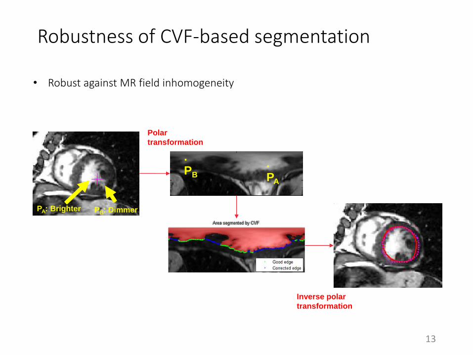
47
• Low contrast area can be recovered regardless of detected LV centroid
PB
.
PC
.
PC
.
PB
.
PB
.
PC
.
PC
PC
.
PB
.
PBPB
PC
Polar transformation
vs.
vs.
Ours
Robustness of CVF-based segmentation

What brings down the success rate?
48
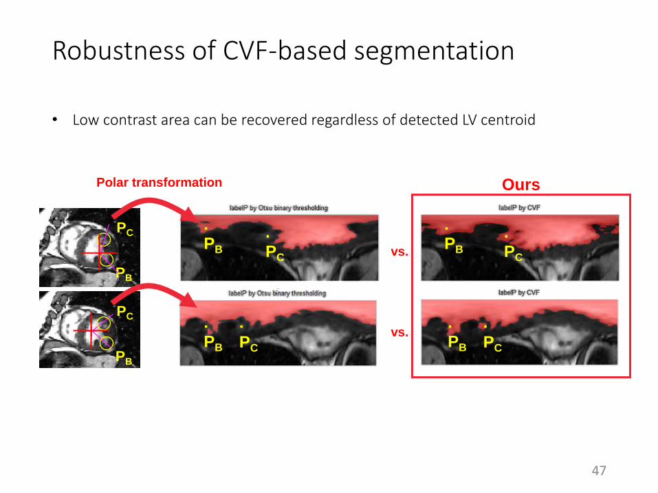
Supplement B:
Extreme case of hypertrophy (SC-HYP-08)
49
-Red: automated. - - - Purple: expert-drawn

What brings down the success rate?
• Mostly in apical slices & extremely hypertrophic hearts.
• Severe partial volume effect in apical slices violates our assumption.
• In hypertrophic cases, endocardium border can be completely obscured by papillary muscle and trabeculae carneae.
50
(A) (B)
Recommended