Quantifying the economicbenefits of paymentmodernization: The case ofthe large-value paymentsystem
payments.ca

Quantifying the Economic Benefits of Payment
Modernization: the Case of the Large-Value Payment System*
Neville Arjani1, Fuchun Li2, and Zhentong Lu3
1Canada Deposit Insurance Corporation, [email protected] Canada, [email protected]
3Bank of Canada, [email protected]
October 18, 2021Abstract
In this paper, we develop a discrete choice framework to quantify economic benefits of
payment modernization in Canada. Focusing on Canadian’s Large-Value Transfer Sys-
tem (LVTS), we first estimate participants’ preference on liquidity cost, payment safety
as well as network effect by exploiting intra-day variations in the relative choice probabil-
ities of the two substitutable sub-systems in LVTS (i.e., Tranche 1 and 2); then we use the
estimated preference to calculate participants’ welfare change when LVTS is replaced
by Lynx (as an important part of the payment modernization initiative) via counterfac-
tual simulations. The results show that 1) comparing to LVTS, Lynx’s liquidity cost and
safety are higher, with the former being a more important factor considered by system
participants; 2) There is an overall welfare gain when over 90% of current LVTS payments
migrate to an Real -Time Gross Settlement (RTGS) system like Lynx, however, it may be
hard to achieve such a highmigration ratio in the newmarket equilibrium; 3)With the equi-
libriummarket share of Lynx, about 75% service level improvement is needed to generate*The authors thank Segun Bewaji, Anne Butler, Cyrielle Chiron, Jonathan Chiu, Walter Engert, Grahame John-
son, Charles Kahn, Andrew McFarlane, and Andrew Usher for helpful suggestions, as well as participants of19th Simulator Seminar (2021) at the Bank of Finland, 2020 BoC-PayCan Quarterly Research Workshop, Bank ofCanada BBL seminar for their useful comments. We also thank Jessica Tropea for English-language editing andproofreading help. The views expressed are ours and not the opinion of any organizations. All errors are ours.

overall net economic benefits to participants. Among other things, adopting liquidity sav-
ingmechanism and reducing risks in the new system can help achieve this improvement;
4) The welfare changes are quite heterogeneous across participants, especially between
large and small ones.
Keywords: Payment Systems, Payment Modernization, Discrete Choice, Economic Benefit.
1

1 Introduction
Payment systems play a crucial role in an economy by providing the mechanisms for con-
sumers, financial institutions, and governments to purchase goods and services, make fi-
nancial investment, and transfer funds. Well-functioning payment systems can enhance the
stability of the financial system, lower transaction costs, promote the efficient use of finan-
cial resources, and facilitate the conduct of monetary policy. Therefore, countries around the
world have devotedmuch effort tomonitoring, regulating, and upgrading their payments sys-
tems with the latest technological developments, international messaging standards, mod-
ernized regulatory and risk control framework.
In Canada, there are currently two core payment systems: the Large Value Transfer System
(LVTS), and the Automated Clearing Settlement System (ACSS). Although these two pay-
ments systems are still functioning well, they were designed more than 20 years ago. As
a result, the outdated technologies, limited functionality and risk control measures indicate
that LVTS and ACSS are not suitable as future foundational platforms for payment clearing
and settlement. Enhancements are required to establish a truly modern payments ecosys-
tem that is fast, flexible, secure, and promotes innovation, and strengthens Canada’s com-
petitive position internationally. To achieve the enhancements, Canada is undertaking a large
initiative to modernize Canadian payments ecosystem. In the modernized world, there will
be three new core payment systems: a Real-Time Gross Settlement System (RTGS) for large
value payments (named Lynx), a DeferredNet Settlement (DNS) system for clearing lower val-
ued and less urgent payments (new batch retail system, formal name not yet determined),
and a real time payment system for processing small value payments (named Real-Time
Rail). The three payment systems will coexist and complement each other to serve their
intended purposes, providing a richer set of viable payment options to meet the Canadian
needs.
Although it is expected that the modernized ecosystem will bring large benefits to Canadian
financial markets and overall economy, very limited work has been done for providing an eco-
2

nomic model-based, quantitative assessment of such benefits.1 Also, payment moderniza-
tion involves substantial investment cost and the new systems might generate new types of
risks. Therefore, it is crucial to provide a quantitative assessment of the potential benefits
brought by the new payment systems, which in turn would provide useful information for the
ongoing payment modernization initiative.
Evaluating the overall benefits of the payment modernization is an ambitious task. Given
the available data, in this paper we take a first step and focus on large value payment sys-
tem modernization, i.e., the replacement of LVTS with Lynx. To do this, we build an empirical
model based on the discrete choice approach for consumer welfare evaluation developed
by McFadden (1981), Small and Rosen (1981), Trajtenberg (1989), Petrin (2002), among oth-
ers. Exploiting the intra-day variations in participants’ system choice behavior recorded in
the historical LVTS and ACSS data, we estimate the payoff function (preference) of each par-
ticipant when sending an inter-bank payment. Then, using the estimated model, we conduct
counterfactual experiments to calculate the welfare changes when LVTS is replaced by Lynx.
A participant (typically a financial institution)’s payoff of sending a payment via a large-value
payment system depends on many factors. As a starter, we consider the two most prominent
ones that govern participants’ key trade-off, i.e., liquidity cost and risk of payment failure (or
delay). To explicitly measure them, we construct two indicators from the characteristics of
both the payment system and the payment in question. These indicators capture payment-
by-payment variations in incentives that FIs face when sending payments. Besides the two
indicators, the payoff of sending a payment also depends on how likely other payments also
use the same system (known as “network effects”), as payment game exhibits clear strategic
complementarity (see among others, Bech and Garratt (2003)). Finally, our model includes
an unobserved, system specific “service quality” level in the payoff function to capture any
residual factors beyond the ones mentioned above.
1One exception is the work by Arjani (2015) who applies discounted cash flow (DCF) analysis to study the potential economic benefits from adopting ISO 20022 payment message standard in payment modernization. However, given the limitation of DCF approach in the estimation of the future cash flows, Arjani (2015) suggests the payments research community to use an economic model-based approach to quantifying the economic ben-efits from payment modernization.
3

Exploiting the special feature that LVTS constitutes effectively two systems, Tranche 1 (T1)
and Tranche 2 (T2), we estimate the payoff function of participants based on their realized
system choices when sending different payments. The key to our estimation strategy is that
the two constructed indicators and the network effect term have sufficient intra-day, payment
level variations to identify their coefficients in the payoff function. With the estimated payoff
function, we calculate a participant’s welfare of sending each payment, and then aggregation
over all payments gives us the total welfare of LVTS.
To evaluate the potential welfare gain, i.e., economic benefit, of the replacement of LVTS
with Lynx, we run a counterfactual simulation by letting all the LVTS payments run through
a baseline, near-RTGS Lynx system and record the output data, especially the two indicators
we constructed. These indicators summarize the key differences between Lynx and LVTS
along the two dimensions: liquidity cost and payment risk. Also, since the network effect in
the payoff function depends on the aggregate outcome (choice probabilities of systems), we
re-calculate the new equilibrium choice probability of Lynx. Finally, we can calculate the total
welfare of Lynx and compare with that of LVTS under alternative assumptions on equilibrium
adjustment, service quality improvement, etc.
Our results show that: 1) Comparing to LVTS, Lynx’s liquidity cost is higher and payment risk
is lower, with the former being a more important factor considered by system participants.
2) The choice of large-value payment systems exhibits rather strong network effects, which
means it is important to take equilibrium adjustment into account when LVTS is replaced
by Lynx. 3) The net economic benefit of Lynx Track changes is on over LVTS depends cru-
cially on the payments migration from LVTS to Lynx and changes in the unobserved service
quality level. In particular, we find that there is an overall welfare gain to participants if over
90% of current LVTS payments migrate to Lynx, which seems unlikely given our equilibrium
adjustment calculation, or Lynx makes a 75% improvement over LVTS in terms of service
quality. For example, adopting a liquidity-saving mechanism (LSM) and/or reducing credit
risk (because Lynx is moving towards a RTGS system) in the system can help achieve this
improvement. 4) The welfare changes are heterogeneous between large and small partici-
4

pants: smaller participants tend to have less welfare gain (or more welfare loss) than large
ones when LVTS is replaced by Lynx.
The rest of the paper is organized as follows. Section 2 provides background information
on LVTS and its modernized version, Lynx. Section 3 describes historical payment data used
in this paper. Section 4 proposes two indicators to quantify the liquidity cost and perceived
risk of delay that a participant faces when sending a payment. In Section 5 we present an
empirical model of the participant’s choice of payment systems. The estimations results of
the model are presented in Section 6. The economic benefits from Lynx are computed and
analyzed in Section 7. Section 8 concludes.
2 Payment Modernization: Large-Value Payment Systems
A pivotal part of the current payment modernization initiative in Canada is the replacement
of the current large-value payment system, LVTS, with its modernized version Lynx. In this
section, we briefly summarizes background information of the LVTS and Lynx.2 This will
help us to identify the key changes experienced by participants when moving from the LVTS
to Lynx, which will be used to set up our model for quantifying the economic benefits of
replacing the LVTS with Lynx.
2.1 The Legacy System: LVTS
The LVTS is Canada’s core electronic payment system for processing inter-bank, large-value
payments. It is the only systemically important payment system in Canada that is operated
by then Payments Canada and overseen by the Bank of Canada (BoC). During the period of
this study, the LVTS has 17 direct participants, including the BoC.3 LVTS consists of two sub-2In Canadian payment modernization program, the current two core payment systems (ACSS and LVTS) and
future three core payment systems (RTR, new batch retail system, and LVTS) differ from each other in a variety of ways. See Kosse et al. (2020) for a detailed summary of their main attributes.
3The direct participants include Big 6 banks, BoC, Laurentian bank, Manulife bank, foreign banks with branches in Canada (State Street Bank, Bank of American, BNP Paribas, HSBC, ICIC), the Largest co-operative movement in Canada (Caise Desjardins) and a provincially owned deposit-taking institution (Alberta Treasury Branches) as well as a credit union consortium (Credit Union Central of Canada). Any deposit-taking institution and member
5
systems, Tranche 1 (T1) or Tranche 2 (T2). A participant can choose either T1 or T2 when
sending a payment. The designs of T1 and T2 are rather different, especially in their distinct
collateral requirements and risk control measures.
For T1, a participant can send a payment as long as its net debit position (assuming the
current payment is made), calculated as the difference between all of its T1 payments sent
(including the current payment) and those received, is no greater than the collateral that the
participant has pledged to the BoC for backing up its T1 payment activities. If the partici-
pant defaults on its LVTS settlement obligations, the collateral will be used to cover any net
negative position in T1. For this reason, T1 payments are known as “defaulter pays”.
In T2, each participant grants Bilateral Credit Limits (BCLs) to every other participant at the
beginning of each day, i.e., the largest net exposure that it is willing to accept with respect to
that participant. In addition, each participant is subject to a multilateral net debit cap, calcu-
lated as the sum of all BCLs extended to it and then multiplied by a specified system-wide
percentage (SWP, currently set at 30%) set by BoC. The multilateral net debit cap (T2NDC)
represents the maximummultilateral net debit position that the participant can incur against
all other participants during the trading day. Each participant pledges collateral to the BoC
equal to the largest BCL it has extended to any other participants multiplied by the SWP. If
a participant defaults on its final settlement obligation, the collateral pool is used to cover
the defaulter’s remaining amounts.4 For this reason, T2 payments are referred as “survivor
pays”.
From the above description, we can see two key differences between T1 and T2 that are
generally perceived by participants: T1 is more resilient to credit risk but more costly in terms
of liquidity than T2, because every payment needs to be fully collateralized in order to be
processed (Kosse et al. (2021)). On the other hand, T2 uses liquidity more efficiently but it
has higher credit risk because of uncollateralized BCLs in T2. As a result, participants have
of the Payments Canada can be a member of LVTS so long as they maintain an account with the BoC and havethe facilities to pledge collateral in LVTS. Deposit-taking institutions that are not members of LVTS must send(or receive) their payments through one of the direct participants.
4In the event of a participant default, the losses of surviving participants are determined based on the BCLthat have granted to the defaulter (Arjani and McVanel (2006))
6

to take this key trade-off of the two sub-systems into account when sending payments.
2.2 The Modernized System: Lynx
Lynx, replacing the LVTS, is the new high-value payments system for processing large value,
time critical payments. One of the significant changes whenmoving from the LVTS to Lynx is
the change in the financial risk model. The financial risk model in Lynx is intended tomitigate
credit risks.5 To achieve this objective, lynx will be a RTGS system and, as such, credit risk
exposure in Lynx will be fully covered by its participants and no longer rely on either the
“survivors-pay” collateral pool or the residual guarantee from the BoC.6
However, the reduction of credit risk in Lynx is traded off against a substantial increase in
intraday liquidity requirements. As a result, to manage liquidity requirements, Lynx will offer
two distinct mechanisms, liquidity savings mechanism (LSM) and urgent payment mecha-
nism (UPM). Lynx’s LSMwill enable participants to delay a payment and to reduce the amount
of liquidity required to settle payments because it uses a combination of queuing, intraday
liquidity recycling, and payment offsetting. For payments that must be settled without delay,
participants may use Lynx’s UPM.
Comparing to the LVTS, since every payment sent through T1 needs to be fully collateralized,
Lynx is rather similar to T1. Moreover, since most LVTS payments are sent through T2 (see
Kosse et al. (2021)), the shift from the LVTS to Lynx implies an overall increase in liquidity cost
and a decrease in credit risk. We shall use an economic model-based approach to conduct
a quantitative analysis of how the replacement of the LVTS with Lynx will affect the overall
welfare of the participants of Canadian large-value payment system.5Note that themitigation of the credit risk in Lynx does notmean that Lynx eliminates systemic risk completely.
In fact, an important systemic risk concern in Lynx is the risk of a liquidity shortage, which may trigger systemicrisk, e.g., gridlock of the whole system.
6In the exceptional event of multiple participant defaults, if the collateral provided by surviving participant toensure settlement in the event that another participant is in default, in addition to the collateral apportioned bythe defaulters, is still not sufficient to cover the value of the final net debit positions of the defaulting participants,the BoC will provide a guarantee of settlement for the remaining amount.
7

3 Data
3.1 Data Source
Ourmain data set consists of information about payments that the direct systemparticipants
processed through the LVTS in 2019. For each payment, we observe its value, exact timing
(date, hour and second), sender, receiver and which tranche it is sent through: T1 or T2. Also,
we observe each participant’s intraday credit limits in both T1 and T2, which are determined
by the amount of pledged collateral and the rules of the LVTS, at any time during each trading
day. Based on the payment level transaction data and participants’ credit limits in T1 and T2,
we will construct intraday time-varying indicators that can capture the key incentives, i.e.,
liquidity cost and risk of payment failure, that participants face when sending payments.
Payments made to the BoC are mostly sent through T1 because of the small BCLs granted
by the BoC. As this is limiting participants’ freedom of choice (thus cannot reveal FIs’s true
preferences), we have excluded payments sent to the BoC from the data and analyses. We
also exclude payments that are less than CAD 10 as these are mostly test payments.
We supplement the LVTS data with ACSS data, which contains daily aggregated, bilateral
payment values and volumes sent through ACSS in 2019, broken down by different pairs of
participants.
The ACSS data will be used to construct a proxy for the market share of the “outside option”
(besides the options T1 and T2) in our estimation of the discrete choice model.
3.2 Data Description
When participants send payments through LVTS, they have to make decisions regarding to
where to send their payments, T1 or T2. These realized decisions provide us information to
build a measure of the relative usage of T1 versus T2, i.e., the share of the transactions in
T1 relative to all transactions in LVTS. Specifically, the share can be calculated as the ratio
between the total volume (value) of payments sent through T1 and the total volume (value)
in LVTS.
8

If the share is close to zero, meaningmost payments are processed in T2, it means that LVTS
operates at a high level of bilateral trust that allows to overcome need for costly collateral. As
the share increases, it signals that the bilateral trust decreases and counter-parties require
more collateral against credit risk. In particular, an unexpected fast transition of the share
from low to high warns a strong risk signal because participants might not have enough
collateral to make payments.
In Figure 1, we plot the volume share of T1 in each of 100 groups of payments, where the
groups are defined by the percentiles of value distribution of all the LVTS payments in 2019.
Two clear facts stand out from this figure. First, the overall usage of T1 is much less frequent
than T2. This indicates that the credit-based transactions (i.e., T2 transactions) relative to all
transactions are quite high, implying that on average for the given sample period, the LVTS
maintains an extremely high level of efficiency of liquidity usage across different percentiles
of the value distribution. Second, T1 is usedmostly for very high value payments. In particular,
this figure shows that there is a relatively low value share of T1 for payments below 71%
percentile. However, the patterns of payments above the 96% percentile shows fairly high
level of usage of T1, suggesting that participants are even more concerned with the safety
when processing very high value payments. Basically these observations show that given
the trade-off between efficiently using liquidity and safely processing payments, participants
face very different incentives when sending payments with different value sizes.7
Similarly, the value share of T1 for per hour varies over the course of a day in a fairly pre-
dictable pattern. The average hour-by-hour pattern of the value share of T1 in a day is re-
ported in Figure 2, which exhibits the timing pattern of the value share of T1 in a day. This
figure indicates that in general T1 is used more heavily in the afternoon than in the morning,
especially in the last two hours before the system is closed. The pattern of the afternoon
peak in the value share of T1 suggests that participants are more concerned with payment
safety and thus switch from T2 to T1 when getting closer to the end of day, i.e., the close time7This pattern of payments is also documented in Kosse et al. (2021). Using the transaction data in the LVTS
from 2004 to 2018, Kosse et al. (2021) find that the large majority of payments in the small and medium valueof percentile bins are sent through T2, The share of T1 payments, however, starts to increase as the transactionvalues get bigger.
9

of the system.
Besides the LVTS data, we also need information about the payment activities outside the
LVTS. This helps us to measure how substitutable the LVTS is to alternative payment sys-
tems, or other payment methods more generally. Since obtaining a comprehensive data set
on all payment systems/methods in Canada is virtually impossible, we focus on the most di-
rect substitute of the LVTS, the ACSS system, for which we have rather good data. Of course,
focusing on the ACSS can potentially understate the “competition” that the LVTS is facing
from other systems; we shall discuss the implications to our model and results later.
Now we turn to the ACSS data. Comparing to LVTS, ACSS is designed for payments with
smaller value and less urgency. Thus ACSS is more substitutable to smaller-value payments
in LVTS. To capture this substitution pattern, we divide the total value of ACSS in 2019 by the
mean value of LVTS payments in each percentile bin (as shown in Figure 1). This gives us
a “normalized volume” of ACSS that is comparable to LVTS payments in a given percentile
bin. Figure 3 shows the share of normalized volume of ACSS (relative to LVTS and ACSS
combined) for each value percentile bin. Note that this construction of outside option in-
deed captures the substitution pattern that ACSS is more substitutable to LVTS for smaller
payments.
4 Liquidity Efficiency and Payment Safety
Credit risk mitigation in T1 is at the cost of high liquidity usage, while a high efficiency of liq-
uidity usage in T2 is at the expense of a high credit risk. Moreover, the high cost of accessing
to liquidity in T1 can increase its exposure to liquidity risks.8 Hence, the liquidity cost and risk
(liquidity and/or credit) are the two key factors that a decisionmaker has to take into account
when sending a payment. In this section, we will propose two indicators that will be used as
proxy variables for the liquidity cost and risk of processing a payment in our empirical model.8Since access to liquidity is costly for settling payments in T1, there is potential (driven by the incentive of par-
ticipants) underprovision of intraday liquidity, and as result, delays or rejections in the settlement of transactions?.
10
4.1 Liquidity Cost Indicator
Given that the payment i can pass the risk-control tests in the payment system j, where j ∈
{T1, T2}, the liquidity cost indicator, which measures the liquidity cost of settling payment i
in terms of the amount of collateral, is defined as,
LCIi,j = ϕi,j ·max {Vi −NIi,j , 0} , (1)
where Vi is the value of payment i,NIi,j is the cumulative net payment income up to payment
i in the current payments cycle in system j, ϕi,j is a cost factor measuring liquidity cost in
terms of collateral spending. Given the design of the LVTS, if the payment i was processed
in T1, ϕi,T1 equals to 1, i.e., $1 collateral is required for spending $1 credit line (Arjani and
McVanel (2006)). If the payment i is processed in T2, ϕi,T2 is defined as MaxASOi,T2
T2NDCi,T2, i.e.,
how much collateral on average is required for spending $1 line of credit.9
The intuition behind the liquidity cost indicator in (1) is straightforward. For any payment i, if
NIi,j is greater than Vi, then sending the payment does not cost any pledged collateral, i.e.,
the cost is 0. WhenNIi,j is less than Vi, the balance Vi −NIi,j need to be paid by collateral,
with different cost factors ϕi,j for T1 and T2, respectively. Similar indicators are proposed
and used in previous literature, see among others, the recent report of CPMI (2015).
4.2 Safety Indicator
From the sender’s point of view, the main risk of sending a payment is that it may be rejected
or delayed due to lack of liquidity. So each participant monitors its intra-day liquidity position
closely to make sure it has sufficient payment capacity (depends on available liquidity) to
stay “safe”, which usually means keeping enough distance away from violating certain risk
control criteria. In the following, we shall construct a payment-specific indicator that mea-
sures sender’s perceived safety regarding payment capacity for the rest of the day after the9MaxASOi,T2 is the largest BCL that participant i chooses to grant to any other participant, multiplied by the
SWP, which is currently set at 30%. T2NDCi,T2 represents the maximum multilateral T2 net debit position thatparticipant i can incur in relation to all other participants in T2 (Arjani and McVanel (2006)).
11
payment is made. For T1, we build on the liquidity risk indicator proposed in Arjani et al.
(2020) and define the safety indicator as
SIi,T1 =NIi,T1 + CLi,T1 +RPIi,T1
RPDi,T1 + Vi, (2)
whereCLi,T1 denotes the intraday credit limits of the sender in the day of payment i,RPIi,T1
is the sender’s payment income to be received from other participants in the remainder of
the day after payment i, and RPDi,T1 is the intraday liquidity demand during the remainder
of day.
Assuming the sender can perfectly predict payment income and demand for the remainder of
the day,10 a greater safety indicator means that the sender is less likely to encounter liquidity
shortage after sending payment i. Hence, the indicatormeasures sender’s expected payment
capability for the remainder of the day. Note that the safety indicator resembles the notion of
“clearing capacity” proposed by ?, which measures the value of payments that a participant
can send under the design of a payment system.
In T2, besides themultilateral credit limit as in T1, senders are subject to bilateral credit limits.
So for any payment i, the sender’s perceived safety level depends on both multilateral and
bilateral liquidity positions. Hence, we extend the safety indicator for T1 to account for both
credit limits, i.e., the safety indicator of payment i in T2 is defined as
SIi,T2 = min
{NIi,T2 + CLi,T2 +RPIi,T2
RPDi,T2 + Vi,BNIi,T2 +BCLi,T2 +BRPIi,T2
BRPDi,T2 + Vi
}, (3)
where the first part in the brackets is the multilateral safety indicator analogous to SIi,T1 and
the second part is the bilateral version with all the variables defined by the sender’s liquid-
ity position with respect to the receiver of payment i, i.e., BNIi,T2, BCLi,T2 BRPIi,T2 and
BRPDi,T2 are the sender’s bilateral net payment income from the receiver, bilateral credit
limit, bilateral payment income to be received from the receiver and liquidity demand from
the receiver for the remainder of the day, respectively.10The extension to allow forecasting errors in the indicator is left for future research.
12

Comparing with SIi,T1, SIi,T2 is smaller given the same multilateral liquidity safety indicator
in T1 and T2, because of the additional bilateral constraints. Also, SIi,T2 has richer variations
as it depends on the receiver of the payment in question. Moreover, given that the different
designs (i.e., risk controls) of T1 and T2 are targeting at liquidity and credit risks respectively,
SIi,T1 mostly captures liquidity risk while SIi,T2 largely reflects credit risk associated with
payments.
5 Model
For a given intended payment i between two participants, deciding which payment system
for settling the payment is a discrete choice problem. Based on the standard demand esti-
mation framework developed by Berry et al. (1995) (hereafter BLP), we propose a discrete
choice demand model for the participants’ decisions on which payment system to use for a
payment. The estimated model will be informative about participants’ preferences and thus
can be used to assess the economic benefits from the replacement of LVTS with Lynx.
To begin with, let J = {T1, T2, 0} denote the choice set of payment systems that the de-
cision maker of each payment i 11 can choose from for settlement, where the alternative 0
represents the “outside option”, i.e., the option of not choosing either T1 or T2, which includes
using alternative systems, e.g., ACSS, for the settlement, delaying or canceling the current
payment for the next cycle, etc.
To map the discrete choice framework to the LVTS payments data, we group similar pay-
ments together by defining a series ofmarkets, where amarketm is defined as a combination
of “hour-sender-receiver-value percentile.” Given the definition of market, we can aggregate
all the payments in amarket (these payments are “similar” in termsof timing/sender/receiver/size)
to obtain the total volume of T1 and T2 in the market. The volume of outside option is con-11In fact, the decision on which system to use is jointly made by the sender and receiver of the payment. For
simplicity, we do notmodel the details of the joint decision process, but regard the sender and receiver collectivelyas one single entity and focus on their final joint decision on which payment system to be used. This single entityis defined as the decision maker. For payments processed in LVTS, the decision mostly dominated by the senderbut we do not want to restrict the interpretation of our model to the sender’s choice problem.
13

structed as in Section 3.2 based on ACSS data. The volume shares of T1, T2 and the outside
option correspond to the market shares implied by our discrete choice model, which mea-
sure choice probabilities of payment systems in the market m, and are the main outcome
variables of our discrete choice model.
Note that with the above specification, we abstract away from the timing decision of send-
ing a payment, which rules out the possibility of strategic delay. The disadvantage of this
approach is that in a counterfactual scenario where the environment changes, our model
cannot predict how timing decisions change. Incorporating these more complicated deci-
sions into the model seems challenging and is beyond the focus of this paper and thus left
for future investigations.
Given the choice set of payment systems,J = {T1, T2, 0}, a decisionmaker’s optimal choice
is determined by its preference, which is represented by a random payoff function. Specifi-
cally, for each payment i in marketm, the random payoff to the decision maker (i.e., referring
to sender and receiver collectively) of sending it through system j ∈ {T1, T2, 0} is specified
to follow a nested-logit structure:
πi,j,m = αLCIj,m + βSIj,m + γsj,m +Xmρ+ ξj,m + ζi,g,m + (1− λ)εi,j,m, (4)
where
• LCIj,m is the log of value-weighted average of liquidity costs of all the payments inm
and SIj,m is log of value-weighted average of safety indicator inm.
• sj,m is the total market share of system j in the “neighboring markets ofm”, defined as
markets with the same sender asm but with different “receiver-hour-value percentile”.
This variable captures the sender’s overall preference for a particular payment system.
The preference could be driven by the economy of scale of using one payment system,
or the expected benefits frompayments coordination in one payment system, i.e., other
participants also use the same payment system. The later is due to the well-known
strategic complementarity in payment games, see, among others, Bech and Garratt
14
(2003)), which is called “network effect” or “social interaction” effect in newtork and
social interaction literature (see, among others, Brock and Durlauf (2001)).
• Xm is a vector of observed market specific characteristics, including the dummy vari-
ables for each sending participant, receiving participant, value percentile, and hour (in
a day).
• ξj,m represents an unobserved characteristic of the payment system j in marketm. It is
important to include this system- andmarket-level demand shock in themodel because
it is impossible to include all the factors affecting the demand for option j in market
m, see, among others, Berry et al. (1995) for detailed justifications for the importance
of this term. In our context, ξ may include factors that are not captured by LCIj,m,
SIj,m,sj,m, and Xm, e.g., service level of a payment system, operational and legal risks
that participants face in a payment system, etc.
• ζi,g,m + (1 − λ)εi,j,m is the preference shock following the nested-logit structure with
λ ∈ [0, 1) being the nesting parameter to be estimated. In particular ζi,g,m is an extreme
value random variable to capture the interaction between the decision maker of send-
ing payment i and the nested group of payment systems, {0} and {T1, T2}, which are
labeled by g = 0 and g = 1, respectively. And εi,j,m is an extreme value variable and is
identically and independently distributed.12
The nested-logit structure is important for modeling the substitution patterns between the
three options in the choice set. The nesting parameter λ in this model can be interpreted
as a measure of substitutability of alternative payment systems across groups.13 As the
parameter λ approaches one, the within-group correlation of payoff levels goes to one. On
the other hand, as λ approaches zero, the within group correlation goes zero, and thereby the
nested logit model is reduced to the logit model. In our case, the substitution between T1 and12In the nested-logit specification, the variable ζi,g,m is a common variable to all systems in g. ? shows that
the distribution of ζi,g,m is the unique distribution with the property that, if εi,j,m is an extreme value randomvariable, then ζi,g,m + (1− λ)εi,j,m is also an extreme value random variable.
13See, among others, Trajtenberg (1989) for details.
15

T2 is naturally stronger than that between T1 (or T2) and the outside option . Therefore, the
nested logit model specified above allows us to model a more realistic substitution pattern
among the three options in the choice set than the simple logit model, which suffers from
the well-known drawback of the independence of irrelevant alternatives property.
Given the randompayoff in (4), we denote themeanutility level of payment system j inmarket
m as,
δj,m = αLCIj,m + βSIj,m + γsj,m +Xmρ+ ξj,m, (5)
which will play an important role to derive the market shares of payment system j. Note that
it is also in a regression form and will be convenient for estimation. Aggregating individual
choices for each system j in group g, we obtain the within-group share of g in marketm,
sj|g,m =eδj,m/(1−λ)
Dg, (6)
whereDg =∑
j∈Ggeδj,m/(1−λ) and Gg includes options in group g.
Similarly, we canobtain themarket share of each payment system j in the choice set {T1, T2, 0}:
sj,m =eδj,m/(1−λ)
Dλg [∑
gD(1−λ)g ]
. (7)
Based on (5), (6), and (7), with δ0,m being normalized to zero, we apply the well-known choice
probability inversion formula of the nested logit model (see Berry (1994)) to obtain the fol-
lowing regression equation:
log
(sj,ms0,m
)= αLCIj,m + βSIj,m + γsj,m + λ log
(sj|g,m
)+Xmρ+ ξj,m, (8)
where sj,m is the observed market share of j in market m and sj|g,m is the observed within-
group market share of j in marketm. Equation (8) forms the basis of estimating the param-
eters in the model.
To estimate (8), we need to impose statistical assumptions on the demand shock ξj,m. Fol-
lowing Berry (1994) and Berry et al. (1995), we assume that the followingmean independence
16

condition holds:
E [ξj,m|Zj,m] = 0, (9)
where Zj,m is a set of exogenous variables that it do not depend on ξj,m.
The twomarket share variables on the RHS, sj,m and log(sj|g,m
), in (8) are clearly endogenous
because they depends on themarket shares on the LHS. Thus we will construct instrumental
variables for them below. Regarding to other RHS variables,Xm is determined by exogenous
payment demand from the outside the systemand thus unlikely to be correlatedwith ξj,t; both
LCIj,m and SIj,m can depends on the market shares in market m as well as its neighbors
(and thus ξ’s), however, we think such dependence is weak after controlling for sj,m directly
(assuming the dependence of LCIj,m and SIj,m on market shares mostly go through sj,m).
In this sense, from the pure econometric point of view, the inclusion of sj,m in our model can
be regarded as away to control the endogeneity ofLCIj,m and SIj,m. Hence, we treatLCIj,m
and SIj,m as exogenous variables and only handle the endogeneity problem in market share
variables.
Specifically, for the two endogenous variables sj,Bm , log(sj|g,m
), we construct the following
instrumental variables: sj,B′m\Bm
,1
|Mm|∑l∈Mm
log(sj|g,l
) , (10)
where B′m is a superset of Bm (a bigger neighbor of market m), Mm is a set of markets
“adjacent” to market m (excluding m itself), i.e., those having the same sender, submission
hour, and value percentile, but different receiver. The construction of these instrumental vari-
ables is based on the following two ideas. First, the market shares of T1 and T2 in neighbor-
ing markets are informative about those in the market considered (i.e., relevance). Second,
the demand shocks in neighboring markets have limited correlation with that in the market
in question (i.e., exogeneity). With the constructed instrument variables in (10) (along with
other exogenous variables), we can estimate (8) using the standard two stage least-squares
method.
17

6 Estimation Results
Table 1 reports the estimation results of the discrete choice model introduced in the pre-
vious section, with four alternative specifications. These specifications are a simple logit
specification, a simple logit specification with fixed effects, a nested logit specification, and
a nested logit specification with instrumental variables. For convenience, we refer to the first
as Logit, the second as FE Logit, the third as Nested Logit, and the fourth as IV Nested logit.
The advantage of presenting the logit results is that we can explore the effects of controlling
for the fixed effects. We present the Nested Logit results to examine the effectiveness of the
instrumental variables for the log of within-group share(sj|g,m
)in the nested logit specifica-
tion.
In the first column of Table 1, we report the estimation results of the simple logit model.
Although the coefficients of safety indicator and network effect are of the expected sign, the
positive coefficient on liquidity cost is anomaly, as we would expect liquidity cost to yield
negative marginal payoff. Additionally, the logit model gives an adjusted R2 of 0.712, which
implies that about 29 percent of the variance in mean utility levels is due to the unobserved
characteristics. In the second column of Table 1, we report the estimation results of the FE
Logit model. All the coefficients are significantly different from zero, and have the expected
sign. Also R2 from the FE Logit model is fairly high at 0.903, a significant improvement from
the Logit model. All of these suggest that controlling for fixed effects is critical to obtain
reasonable estimations of the coefficients.
In Table 1, the third column reports the estimation results of the Nested Logit specificiation
using the OLS, while the fourth column reports the results of IV Nested Logit, using the in-
strument variables in (10). Comparing the estimation results in the third column with that in
the fourth column, we find that the coefficients between two columns differ noticeably, es-
pecially the coefficient on the network effect in the fourth column decreases substantially.
This indicates the importance of correcting the endogeneity problem.
Focusing on IV Nested Logit model, our favored specification, we can see that the coeffi-
18

cients on liquidity cost, safety indicator, network effect, and log of the within-group market
share all have expected signs and are statistically significant. Also, the nesting parameter,
i.e., the coefficient of the log of the within-group market share, is greater than .7, indicating a
strong within-group correlation between the preferences for T1 and T2 relative to the cross-
group correlation between T1 (or T2) and outside option 0. Also, the statistically significant
coefficient of the log of the within-group market share suggests that the extension from the
FE logit to the IV Nested Logit seems necessary. Finally, the large value of the first-stage F
test statistic supports the relevance of the constructed instruments.
7 Quantifying the Economic Benefits of Lynx
In this section, we use the estimated discrete choice model in previous section to calculate
the economic benefits of Lynx, which is replacing LVTS as part of the paymentmodernization
initiative.
7.1 Welfare Calculation
The discrete choicemodel allows us to calculate thewelfare, or economic benefits, to partici-
pants fromsending payments. Given our IV nested logit specification, using similar approach
as in Trajtenberg (1989) who suggested the use of discrete choice models to measure the
benefits of product innovations, the expectedmaximum payoff of sending a payment in mar-
ketm under the current LVTS regime is calculated as follows:
EVLVTS,m = log
1 +
(exp
(δT1,m
1− λ
)+ exp
(δT2,m
1− λ
))1−λ , (11)
where δT1,m and δT2,m are the fitted value of mean utilities defined as
δj,m = αLCIj,m + βSIj,m + γsj,Bm +Xmρ+ ξj,m, j ∈ {T1, T2} . (12)
19

Note that these estimated parameters in (11) and (12), λ, α, β, γ, ρ, and ξj,m are obtained from
the estimation results in Section 6.
After LVTS is replaced by Lynx, the choice set of payment systems that participants are facing
becomes {0, Lynx}. And the expected maximum payoff of sending a payment in market m
boils down to:
EVLynx,m = log[1 + exp
(δLynx,m
)], (13)
where δLynx,m is themean payoff of sending a payment through Lynx and can be decomposed
as
δLynx,m = αLCILynx,m + βSILynx,m + γsLynx,Bm +Xmρ+ ξLynx,m. (14)
Note that α, β, γ andXmρ in (14) are the same as in (12), however, other variables in (14) are
unknown and we will discuss how we assign their values in the next subsection.
Given the expected maximum payoffs of both LVTS and Lynx in marketm, we can measure
the welfare change from replacing LVTS with Lynx by the required amount of collateral (in
Canadian dollars), i.e.,
∆EB =∑m
Wm · Volm ·(EVLynx,m − EVLVTS,m
), (15)
where Volm is the total payment volume in marketm, and Wm is a factor that translates the
payoff level of each payment for a payment system into “willingness-to-pay” measured in
terms of collateral (in Canadian dollars). Since the liquidity cost enters the payoff function
in log form, we can define the factor as
Wm =exp (LCIT1,m) + exp (LCIT2,m)
|α|. (16)
It is possible to further translate the collateral amount into actual financial cost (e.g., us-
ing appropriate interest rates), however, this is not straightforward because it can be tricky
to measure collateral cost that varies by participants, timing, etc., and less relevant to our
20

current analysis so we leave it for future investigation.14
7.2 Payoff Function of Lynx
Since Lynx is not launched by the time of this analysis, we do not have realized data from the
newsystem. Hence, we have to construct synthetic data of Lynx using simulation. Simulating
a full-scale Lynx with all its design features is challenging, we focus on a simplified version
of Lynx with only its core characteristics, i.e., it is a real-time settlement system, and each
payment needs to be fully collateralized in order to be processed.
In particular, we let all the payment instructions from the 2019 LVTS data including both T1
and T2 run through the simplified Lynx and record the outcome, e.g., we evaluate the cost and
safety indicators in this new system. In this process, wemaintain the following assumptions:
(1) all the LVTS payments migrate to the Lynx system; (2) the timing and order of all the
payments for each day are kept unchanged; (3) participants pledge sufficient collateral to
Lynx so that they can make all the payments in a fully collateralized manner; (4) the risk
control test for each payment in Lynx is the same as in T1.
Figure 4 shows the comparison between LVTS and Lynx in terms of liquidity cost, for different
hours in a day and different sending participants. As expected, the liquidity cost of Lynx is
higher than that of LVTS. Also, the difference is rather heterogeneous across participants and
different hours. For example, participants with higher overall liquidity cost, mostly driven by
their larger volume of payments, have to bear greater increase in liquidity cost when Lynx
replaces LVTS.
Figure 5 plots the safety indicators for Lynx and LVTS, respectively, across different partici-
pants and hours in a day. It is clear that the safety indicator of Lynx is higher than LVTS,mostly
due to the pooled credit limits (T1 and T2) and the removal of bilateral risk control test of T2
(reflecting the reduction in credit risk). Comparing with the liquidity cost, the safety indicator
is much smaller in scale and thus its difference between Lynx and LVTS will have less effect
on the participants’ welfare changes.14See McPhail and Vakos (2003) for some high-level estimates of the collateral costs in LVTS.
21

With the above simulation, we obtain values of liquidity and safety indicators, LCILynx,m and
SILynx,m, in themean payoff function of Lynx (14). Regarding to the unobserved characteristic
of Lynx, ξLynx, which captures the relative payoff (e.g., service quality level) comparing to the
outside option, we assume it is proportional to the average of its counterparts of T1 and T2,
i.e.,
ξLynx =θ12
(ξT1 + ξT2
),
where θ1 is a tuning parameter capturing the unobserved service quality level of Lynx (com-
paring to the LVTS).
Finally, the model includes a network effect captured by sj,m in (4) that needs to be deter-
mined for Lynx. We consider two ways of assigning the value. First, we simply assume that
it is proportional to the total market share of LVTS, i.e.,
sLynx,m = θ2(sT1,m + sT2,m
),
where θ2 represents the fraction of LVTS payments migrating to LVTS. Second, sLynx,m can
be endogenously determined the equilibrium adjustment of market shares. Specifically, with
the new system Lynx replacing LVTS, the model implies market shares of Lynx that differ
from those of LVTS. Then the network effect term, which depends on the market shares
in neighboring markets, needs to be updated. This change in turn implies a vector of new
market shares of Lynx. This heuristic adjustment process can be formalized as a iterative
approach to compute the new equilibrium market shares of Lynx. Formally, the equilibrium
market shares of Lynx can be computed iteratively as follows:
sr+1Lynx,m =
exp(αLCILynx,m + βSILynx,m + γsLynx,m
(srLynx
)+Xmρ+ ξLynx,m
)1 + exp
(αLCILynx,m + βSILynx,m + γsLynx,m
(srLynx
)+Xmρ+ ξLynx,m
) , (17)
where srLynx is the vector of market shares in the r-th iteration (with some starting value s0Lynx).
This iteration process is in fact a contraction mapping given the value of our estimated pa-
rameter γ = 1.549, see Brock and Durlauf (2001) for details.
22

7.3 Results
We first consider the simple case where θ1 = 1 and there is no equilibrium adjustment, i.e.,
treating the network effect term as exogenous and examining how the network effect con-
tributes to the welfare measure. Figure 6 shows the total welfare change against θ2, the
fraction of payments in LVTS migrating to Lynx. There are three lines in the graph: “Base-
line” refers to the simple Lynx described above; “20% Cost Reduction” is the case where we
assume Lynx adopts certain liquidity saving mechanism such that its liquidity cost is overall
20% lower than the baseline simple Lynx; “100% Safety Increase” refers to the case where
Lynx improves the safety indicator by 100%.
We can see that as θ2 increases, the net economic benefits of Lynx also increases and ex-
ceeds 0 when θ reaches around .9, which means that there is a welfare gain when over 90%
of current LVTS payments migrate to Lynx. Also, lowering liquidity cost by 20% has a non-
negligible effect on welfare, but increasing payment safety indicator can do very little.
Next, we consider the case with equilibrium adjustment. It turns out the new equilibrium im-
plies a lower migration ratio, which is around 55%,15 than 90%. Under this lower migration
ratio, the baseline Lynx is likely to cause a welfare loss to participants, however, a quality im-
provement (e.g., an increase in ξLynx) can mitigate the loss and even generate welfare gains.
Then a natural question is how much quality improvement is needed? Figure 7 illustrates
the overall welfare changes against θ1, the percentage of quality improvement. We can see
that Lynx needs an almost 75% improvement in service level over LVTS to achieve an overall
welfare gain to the participants. Again, lowering liquidity cost (e.g., through liquidity saving
mechanisms) has much larger effects than improving payment safety indicator.
Besides the overall welfare change, we show the heterogeneous effects across participants
in Figure 8 for the special case where θ1 = 1.75 (with equilibrium adjustment), i.e., overall
welfare change is 0. We can see that the welfare changes are rather heterogeneous across15This result is in the same ballpark the payment modernization patterns predicted by Kosse et al. (2021).
However, recall that this result is obtained under the assumption that Lynx is pure RTGS system, which is notexactly the case because of the adoption of liquidity saving mechanisms in Lynx. Hence, we expect that thispredicted migration ratio might be a reasonable “lower bound” for the actual migration ratio that will be realizedin the near future.
23

participants, e.g., Bank 1 (a big participant) enjoys a quite large welfare gain while small
participants as a whole (labeled as “Others”) suffers from a welfare loss. The differences are
mainly driven by the heterogeneous effects of replacing LVTS with Lynx on the random payoff
functions across different participants. This heterogeneous effect raises some interesting
policy questions, e.g., the central bank and payment system operator may consider providing
certain incentives for some participants, which suffers from welfare losses, to participate in
the new system, given that after all participation is vital for the new system to achieve its
public objectives.
8 Concluding Remarks
In this paper, we propose a discrete choice demand framework to model the participants’
decisions on which payment system to use for sending payments and apply it to measure
benefits of payment modernization in Canada. Focusing on the large-value payment system
modernization, we first use historical data of LVTS to estimate participants’ preference on
liquidity cost, payment safety as well as network effect; then we use the estimated preference
to calculate participants’ welfare change when LVTS is replaced by Lynx based on simulation.
Our results suggest that a high migration ratio and/or service quality improvements (e.g.,
new liquidity saving/safety features) are crucial to generate overall net economic benefits to
participants.
Our study is the first step to quantify the economic benefits of payment modernization. There
are several caveats in our current results:
• Weconstruct and include only two indicators describing the incentives that participants
are facing when making a payment. Although they capture two important factors, the
two indicators clearly cannot exhaust all the important considerations that participants
have when making payments. Including more variables capturing the incentives par-
ticipants face can improve our results, although this is not an easy task.
• Our measure of the “outside option” (relative to LVTS) is based on ACSS data. This as-
24

sumption may underestimate the share of actual outside option, especially for small-
value payments, because there are other payment systems/networks available for fi-
nancial institutions to process payments. Whether this would change our conclusion is
not clear. For example, if Lynx has certain new features that can “steal” market shares
from other payment systems, then wewould underestimate the welfare gain of the new
system.
• Our evaluation focuses on the large-value payment system modernization and thus
only covers part of the payment ecosystem. Hence, the welfare results should be in-
terpreted with caution. For example, even if Lynx cannot generate a welfare gain when
replacing LVTS, other modernized payment systems, e.g., the new retail payments may
produce sufficiently high surplus to make the overall benefits of payment moderniza-
tion positive.
• We only measure the economic benefits to participants in the system and do not con-
sider the overall potential benefit or loss to the whole society. Given that payment sys-
tems have clear externalities in terms of systemic risk, it is important to extend the
current analysis along this line.
Despite the above mentioned caveats, which are mostly driven by the data limitations, our
proposed framework for evaluating the economic benefits of payment systems is rather gen-
eral and flexible. With more and richer data in the future, especially data generated by Lynx,
the framework can be extended and enriched to provide a more comprehensive assessments
of the welfare implications of payment modernization.
25
References
Arjani, Neville, “The economic benefit of adopting the ISO 20022 paymentmessage standard
in Canada,” Technical Report, Canadian Payments Association 2015.
andDarceyMcVanel, “A primer onCanada’s large value transfer system,” Technical Report,
Bank of Canada 2006.
, Fuchun Li, and Leonard Sabetti, “Monitoring Intraday Liquidity Risks in a Real Time Gross
Settlement System,” Technical Report, Payments Canada Discussion Paper 2020.
Bech, Morten L. and Rod Garratt, “The intraday liquidity management game,” Journal of Eco-
nomic Theory, April 2003, 109 (2), 198–219.
Berry, S., J. Levinsohn, and A. Pakes, “Automobile prices in market equilibrium,” Economet-
rica: Journal of the Econometric Society, 1995, pp. 841–890.
Berry, S.T., “Estimating discrete-choice models of product differentiation,” The RAND Journal
of Economics, 1994, pp. 242–262.
Brock, William A and Steven N Durlauf, “Discrete choice with social interactions,” The Review
of Economic Studies, 2001, 68 (2), 235–260.
CPMI, “Liquidity efficiency of the large value payment systems around the world,” Technical
Report 2015.
Kosse, Anneke, Zhentong Lu, and Gabriel Xerri, “An economic perspective on payments mi-
gration,” Technical Report, Bank of Canada 2020.
, , and , “An economic perspective on paymentsmigration,” Journal of Financial Market
Infrastructure, 2021.
McFadden, D., “Econometric Models of Probabilistic Choice,” in C. Manski and D. McFadden,
eds., Structural Analysis of Discrete Data with Econometric Applications, Cambridge: MIT
Press, 1981, chapter 5, pp. 198–272.
26
McPhail, Kim and Anastasia Vakos, “Excess Collateral in the LVTS: HowMuch is TooMuch?,”
Technical Report, Bank of Canada 2003.
Petrin, Amil, “Quantifying the benefits of new products: The case of the minivan,” Journal of
political Economy, 2002, 110 (4), 705–729.
Small, Kenneth A and Harvey S Rosen, “Applied welfare economics with discrete choice
models,” Econometrica: Journal of the Econometric Society, 1981, pp. 105–130.
Trajtenberg, Manuel, “The welfare analysis of product innovations, with an application to
computed tomography scanners,” Journal of Political Economy, 1989, 97 (2), 444–479.
27

Tables
Table 1: Demand Estimation Results
Simple Logit Nested LogitWithout FE With FE Without IV With IV
Liquidity Cost 0.564 -0.0443 -0.0220 -0.0299(0.00250) (0.00467) (0.00440) (0.00438)
Safety Indicator 0.0154 0.0246 0.0264 0.0202(0.00248) (0.00187) (0.00181) (0.00180)
Network Effect 6.191 9.788 6.001 1.549(0.0175) (0.260) (0.223) (0.117)
Nesting Parameter 0.515 0.724(0.00775) (0.0218)
Constant -8.140 -7.082 -5.262 -4.522(0.0335) (0.130) (0.123) (0.157)
Sender FEReceiver FEHour FEValue Pctile FECragg-Donald Wald F 7869.96# Obs. 104,707 104,707 104,707 100,350Adj. R2 0.712 0.903 0.909 0.913Note: Table 1 reports the estimation results of the discrete choice model,with four alternative specifications. These specifications are a simple logitspecification without fixed effect, a simple logit specification with fixed ef-fects, a nested-logit specificationwithout IV, and a nested-logit specificationwith IVs. The standard errors of the estimated parameters are reported inparentheses. All the estimates shown in the table are statistically signifi-cant at 1% significant level.
28

Figures
Figure 1: Volume Share of T1 for Different Payment Sizes
Note: Figure 1 plots the volume share of T1 in each of 100 groups of payments, where the groups are defined bythe percentiles of value distribution of all the LVTS payments in 2019. In each group, the volume share iscalculated as the ratio between the total volume of payments sent through T1 and the total volume throughLVTS.
29

Figure 2: Value Share of T1 for Different Hours
Note: Figure 2 plots the average hour-by-hour pattern of the value share of T1 in a day. In each hour, the valueshare is calculated as the ratio between the total value of payments sent through T1 and the total value ofpayments through LVTS.
30

Figure 3: Volume Share of Outside Option
Note: Figure 3 shows the share of normalized volume of ACSS in 2019 (relative to LVTS and ACSS combined)for each value percentile bin.
31

Figure 4: Liquidity Cost: LVTS vs Lynx
Note: Figure 4 shows the comparison of liquidity cost between LVTS and Lynx in 2019, for different hours in aday and different sending participants.
32

Figure 5: Safety Indicator: LVTS vs Lynx
Note: Figure 5 plots the safety indicator for Lynx and LVTS, respectively, across different participants and hoursin a day.
33
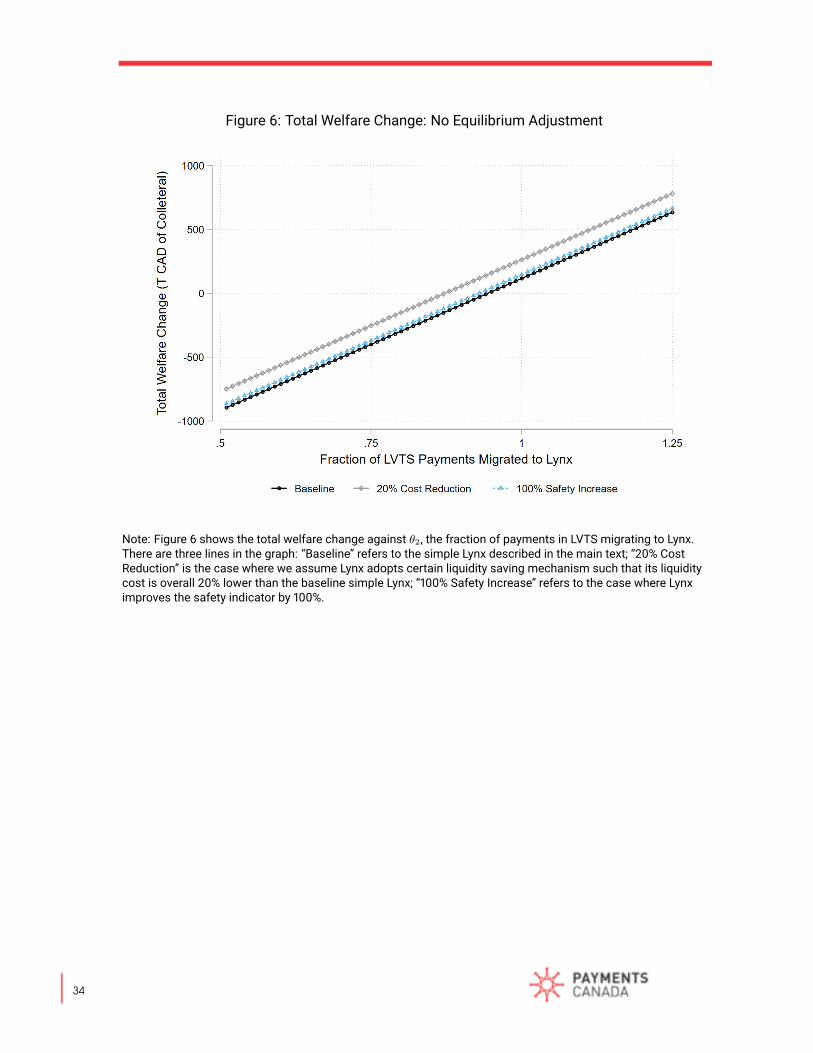
Figure 6: Total Welfare Change: No Equilibrium Adjustment
Note: Figure 6 shows the total welfare change against θ2, the fraction of payments in LVTS migrating to Lynx.There are three lines in the graph: “Baseline” refers to the simple Lynx described in the main text; “20% CostReduction” is the case where we assume Lynx adopts certain liquidity saving mechanism such that its liquiditycost is overall 20% lower than the baseline simple Lynx; “100% Safety Increase” refers to the case where Lynximproves the safety indicator by 100%.
34

Figure 7: Total Welfare Change: With Equilibrium Adjustment
Note: Figure 7 illustrates the overall welfare changes against θ1, which is a tuning parameter capturing theservice level improvement of Lynx.
35

Figure 8: Welfare Change: Heterogeneity Across Banks
Note: Figure 8 shows the heterogeneous welfare changes across participants for a given level of the tuningparameter capturing the service quality of Lynx, i.e., θ1 = 1.75, at which the overall welfare change is 0.
36
Recommended