Czech Technical University in Prague
Faculty of Electrical Engineering
Department of Control Engineering
BACHELOR THESIS
Quadratic Programming Algorithmsfor Fast Model-Based Predictive Control
Prague, May 2013 Ondřej Mikuláš


Abstract
This thesis deals with quadratic programming (QP) algorithms for the use in fast model
based predictive control applications. First, general overview of model based predictive
control and quadratic programming is given. Then, several QP algorithms – active set
method, fast gradient method and interior point method – are described.
Then, these algorithms are tested on model predictive control example and on ran-
domly generated QPs. We treat especially computation time required to obtain a solu-
tion, the factors that influence the run-time (condition number, correction horizon etc.)
and also the typical properties related to the computation time of the above mentioned
algorithms.
Finally, the thesis deals with robust control performance of model predictive controller
without constraints. With selected plants, the effect of plant model mismatch on the
robust quality of control is studied in conjunction with correction horizon length.
Abstrakt
Tato práce se zabývá algoritmy kvadratického programování (QP) pro nasazení v rychlých
aplikacích prediktivního řízení. Nejprve je podán obecný pohled na prediktivní řízení
a kvadratické programování. Poté jsou představeny některé algoritmy QP – konkrétně
metoda aktivních množin, rychlá gradientní metoda a metoda vnitřního bodu.
V další části jsou tyto algoritmy otestovány na příkladu prediktivní regulace a také po-
mocí náhodně generovaných QP. Důraz je kladen především na potřebnou dobou výpočtu
a na to, jak je tato doba ovlivněna různými faktory (podmíněnost, korekční horizont a
další) a jaké jsou typické vlastnosti uvedených algoritmů co se této doby týká.
Nakonec se práce věnuje robustnosti prediktivního regulátoru ve smyslu kvality řízení
bez přítomnosti omezení. Na konkrétních soustavách popisuje vliv chybného modelu na
kvalitu řízení v souvislosti s délkou korekčního horizontu.


Acknowledgments
I would like to express many thanks to Vladimír Havlena for the supervision of my thesis
and for the time he devoted to me. Next, many thanks come to Ondřej Šantin for many
indispensable consultations. Last but not the least, let me thank to my family for their
endless support during my studies.
Poděkování
Na tomto místě děkuji Vladimíru Havlenovi za vedení mé bakalářské práce a za čas který
mi věnoval. Děkuji také Ondřeji Šantinovi za bezpočet konzultací, bez kterých by tato
práce nebyla taková jaká je. Nakonec mi dovolte poděkovat mé rodině za jejich bezmeznou
podporu v celém průběhu mého studia.


Contents
1 Introduction 1
1.1 Basic principle of predictive control . . . . . . . . . . . . . . . . . . . . . . . 1
1.2 Brief history . . . . . . . . . . . . . . . . . . . . . . . . . . . . . . . . . . . . 2
1.3 Predictive control at present . . . . . . . . . . . . . . . . . . . . . . . . . . . 2
2 Model based predictive control 5
2.1 Predictive control algorithm . . . . . . . . . . . . . . . . . . . . . . . . . . . 5
2.1.1 Prediction . . . . . . . . . . . . . . . . . . . . . . . . . . . . . . . . . 5
2.1.2 Receding horizon . . . . . . . . . . . . . . . . . . . . . . . . . . . . . 6
2.1.3 Move blocking . . . . . . . . . . . . . . . . . . . . . . . . . . . . . . 7
2.1.4 Cost function and optimization . . . . . . . . . . . . . . . . . . . . . 7
2.1.5 Constraints . . . . . . . . . . . . . . . . . . . . . . . . . . . . . . . . 8
2.2 Regulator . . . . . . . . . . . . . . . . . . . . . . . . . . . . . . . . . . . . . 10
2.3 Reference tracking . . . . . . . . . . . . . . . . . . . . . . . . . . . . . . . . 11
2.3.1 State space model to include references . . . . . . . . . . . . . . . . 11
2.3.2 Output and tracking error . . . . . . . . . . . . . . . . . . . . . . . . 11
2.3.3 Cost function . . . . . . . . . . . . . . . . . . . . . . . . . . . . . . . 12
2.4 Offset-free tracking . . . . . . . . . . . . . . . . . . . . . . . . . . . . . . . . 12
2.5 Unconstrained MPC . . . . . . . . . . . . . . . . . . . . . . . . . . . . . . . 14
3 Quadratic programming algorithms 17
3.1 Quadratic programming . . . . . . . . . . . . . . . . . . . . . . . . . . . . . 17
3.1.1 Quadratic program . . . . . . . . . . . . . . . . . . . . . . . . . . . . 17
3.2 KKT optimality conditions . . . . . . . . . . . . . . . . . . . . . . . . . . . 18
3.3 Unconstrained QP . . . . . . . . . . . . . . . . . . . . . . . . . . . . . . . . 19
3.3.1 Gradient descent methods . . . . . . . . . . . . . . . . . . . . . . . . 19
3.3.2 Newton’s method . . . . . . . . . . . . . . . . . . . . . . . . . . . . . 20
3.3.3 Example . . . . . . . . . . . . . . . . . . . . . . . . . . . . . . . . . . 21
3.4 Equality constrained QP . . . . . . . . . . . . . . . . . . . . . . . . . . . . . 21
3.4.1 KKT conditions . . . . . . . . . . . . . . . . . . . . . . . . . . . . . 22
3.5 Inequality constrained QP . . . . . . . . . . . . . . . . . . . . . . . . . . . . 23
3.5.1 Active set method . . . . . . . . . . . . . . . . . . . . . . . . . . . . 23
3.5.2 Fast gradient method . . . . . . . . . . . . . . . . . . . . . . . . . . 25
3.5.3 Interior point method - Logarithmic barrier . . . . . . . . . . . . . . 26

CONTENTS
4 Properties of QP algorithms 29
4.1 QP solvers under test . . . . . . . . . . . . . . . . . . . . . . . . . . . . . . 29
4.1.1 quadprog - Active set method . . . . . . . . . . . . . . . . . . . . . . 29
4.1.2 qpOASES - Specialized active set method . . . . . . . . . . . . . . . 29
4.1.3 FiOrdOs - Fast gradient method . . . . . . . . . . . . . . . . . . . . 30
4.1.4 MOSEK - Interior point method . . . . . . . . . . . . . . . . . . . . 30
4.1.5 Fast MPC - Specialized interior point method . . . . . . . . . . . . . 30
4.2 Numerical experiments . . . . . . . . . . . . . . . . . . . . . . . . . . . . . . 31
4.2.1 Computation time measurement . . . . . . . . . . . . . . . . . . . . 31
4.2.2 Model predictive control example . . . . . . . . . . . . . . . . . . . . 31
4.2.3 Random QP . . . . . . . . . . . . . . . . . . . . . . . . . . . . . . . 36
4.3 Summary . . . . . . . . . . . . . . . . . . . . . . . . . . . . . . . . . . . . . 37
5 Robustness of unconstrained MPC 39
5.1 Influence of uncertain system parameters . . . . . . . . . . . . . . . . . . . 39
5.1.1 Example . . . . . . . . . . . . . . . . . . . . . . . . . . . . . . . . . . 40
5.2 Influence of control horizon . . . . . . . . . . . . . . . . . . . . . . . . . . . 41
5.2.1 Nominal models and controller tuning . . . . . . . . . . . . . . . . . 42
5.2.2 Monte Carlo simulation . . . . . . . . . . . . . . . . . . . . . . . . . 43
6 Conclusion 47
Bibliography 50
Appendices 51
A Contents of the attached CD 51

Chapter 1
Introduction
Model-based predictive control (MPC) is a modern, optimization driven control strat-
egy. It involves a solution of an optimization problem at each time step. Therefore, fast
optimization algorithms are required in order to control fast dynamic systems.
The objective of this thesis is to study the properties of quadratic programming (QP)
algorithms that are suitable for the use in fast model predictive control applications.
Another objective is to illustrate the influence of quadratic programming problem size on
the control quality and robustness of model predictive controller.
The thesis is organized as follows. This chapter presents the basic idea of predictive
control. Next, brief history overview is provided, and finally the state of the art is shown.
The second chapter gives a more detailed description of MPC algorithm. The third chapter
reviews optimization algorithms for QP problems. Namely gradient descent method and
Newton’s method for unconstrained QP, and active set method, fast gradient method and
interior point method for inequality constrained QP.
The fourth chapter analyses the properties of the algorithms from the third chapter.
Especially noted are the factors that influence the computation time. In the fifth chapter
robustness of model predictive controller in terms of control quality is discussed.
1.1 Basic principle of predictive control
Predictive controllers use future system behavior prediction to choose an appropriate ac-
tion. These controllers act a little bit like humans do. A person also predicts the conse-
quence of his or her actions before doing one and usually chooses the best possible.
The prediction is made based on the model of the system and an actual state. So is
the prediction made in our head. We also have to know how the system acts in different
states. The need of the model is natural. When we come to some new situation, we should
get some knowledge about it in order to be able to handle it.
At each time instant, a control action has to be selected, that results in the best pre-
dicted behavior. A cost function is defined to evaluate the cost of the predicted behavior.
The cost function may reflect various things. From the difference between the actual be-
havior and the desired one (tracking error), to the costs of the control or to the violation
of constraints put on the system. Then, a mathematical optimization problem is solved
1

2 CHAPTER 1. INTRODUCTION
to obtain the control action that minimizes the cost function.
This control strategy is in contrast with classical control methods such as PID (propor-
tional, integral, derivative). They do not make any adjustments based on the knowledge
of the system and its future behavior. Typically, tracking error is measured and fed into
the controller. An action is taken by PID only when an error occurs. On the other hand,
predictive controller predicts that an error may occur in the future, so it takes an action
at the moment to prevent it.
The following example is inspired by the one provided in [1]. Consider riding a mo-
torbike. A skilled driver knows how the motorbike acts under various conditions (i.e. the
model) and he also has some kind of cost function. Staying on the road is more important
to him than going at high speed. Of course, different riders have different cost functions.
When he approaches a sharp turn, he makes a prediction of his future trajectory at dif-
ferent speeds and directions. Then, he chooses the best of these actions based on their
predicted cost. After that, he applies the correction and makes another prediction for the
newly occurred situation. This repeats until the driver ends his route.
1.2 Brief history
Time to solve the underlying optimization problem had long restricted the use of MPC
to slow dynamic processes. This includes various processes in petrochemical industry or
chemical industry.
The first industrial applications date back to the late 1970’s. We name for example
Model predictive heuristic control in [2] or Dynamic matrix control in [3]. The earliest im-
plementations of MPC used input/output models (impulse and step response) [4] because
these models are readily available from experiments.
In the late 1980’s Shell engineers introduced an implementation which made use of the
state space process model. This package is called SMOC (Shell multivariable optimization
controller) and it uses grey-box identification to obtain a plant model.
As the digital computers became faster and less expensive, the popularity of MPC
grew. Today, it is a widely accepted and well known control method. Further history
overview can be found in [5, sec. 2].
1.3 Predictive control at present
Today, various types of predictive control are referred to either as predictive control or as
model based predictive control.
Increase in the computational power of hardware, new algorithms and intensive re-
search has led to its wide spread. Even systems with fast dynamics that require short
sampling times can be handled with today’s algorithms and hardware.
MPC formulations can be divided according to norm used in a cost function. First,
l1 and l∞ norms result in linear programming (LP). And second, l2 or Euclidean norm
results in quadratic programming (QP). We restrict our aim to the latter one only.

1.3. PREDICTIVE CONTROL AT PRESENT 3
Significant results in QP algorithms specific to MPC have been reported in [6] (active
set method), [7] (fast gradient method) or [8] (interior point method). These algorithms
will be described in more detail in the following chapters.
Special attention is paid to the operation of MPC on inexpensive hardware (see e.g. [9])
or field-programmable gate arrays (for example [10]).
MPC is much appreciated for its ability to take system constraints (e.g. actuator
limits) into account which makes it suitable for deployment in industrial process control.
It is not restricted to systems with single input and single output and so even large
scale multiple input multiple output (MIMO) systems can be controlled (for a survey of
industrial applications see [5]). The design of a model based predictive controller for such
a MIMO system is quite straightforward.
Notation
• R - set of real numbers
• Lower and upper case italic letters - scalars
• Bold lowercase letters a to z - column vectors in Rn
• Bold uppercase letters A to Z - matrices in Rm×n
• 0 (1) - vector or matrix of zeros (ones) of corresponding size
• I - identity matrix of corresponding size
• AT - matrix transpose

4 CHAPTER 1. INTRODUCTION

Chapter 2
Model based predictive control
This chapter presents more detailed description of model based predictive control algo-
rithm for linear discrete-time systems. First, receding horizon principle is introduced,
then prediction of future system states is shown. After that, the regulator and the track-
ing problems are described. Finally, specialized MPC formulation that allows offset-free
tracking for nominal model with simple box constraints is presented. Great introductory
text on MPC can be found e.g. in [1]. Note that in the following text, only state space
models are considered.
2.1 Predictive control algorithm
Model based predictive controller makes a prediction of future system behavior based on
its model, the current system state, the input trajectory, or a disturbance entering the
system. Then, it selects the best possible input action according to a cost function. To
do this it has to solve an optimization problem, subject to possible constraints. Finally, it
applies the first element of the optimal selected input sequence to the system. At each time
step, this procedure is repeated, which introduces so called receding horizon principle.
We describe these components in more detail in the following subsections.
2.1.1 Prediction
Prediction is a crucial part of a predictive controller. It is based on a model of a system
to be controlled. For the prediction to be correct, the model has to be as exact as possi-
ble, as well as the state measurement or estimation. It enables the controller to predict
consequence of its actions. The prediction is made only for a finite number of steps. This
number is called prediction horizon and it is denoted as np.
Consider a linear time-invariant discrete-time model with n state variables in vector
x ∈ Rn, m inputs in u ∈ Rm and p outputs in y ∈ Rp. Its evolution is described by
xk+1 = Axk + Buk
yk = Cxk + Duk,(2.1)
where A ∈ Rn×n, B ∈ Rn×m, C ∈ Rp×n and D ∈ Rp×m are state space matrices. Now we
5

6 CHAPTER 2. MODEL BASED PREDICTIVE CONTROL
write xk+2 in terms of xk+1 and uk+1 and then substitute from (2.1).
xk+2 = Axk+1 + Buk+1 = A2xk + ABuk + Buk+1,
yk+1 = Cxk+1 + Duk+1 = CAxk + CBuk + Duk+1.(2.2)
Similar procedure can be done for the other future time steps. The resulting time series
can be expressed in a convenient block matrix form. For the predicted system states we
obtain the following:xk+1
xk+2
...
xk+np
︸ ︷︷ ︸xk+1,np
=
A
A2
...
Anp
︸ ︷︷ ︸
Px
xk +
B 0 · · ·AB B · · ·
......
. . .
Anp−1B Anp−2B · · ·
︸ ︷︷ ︸
Hx
uk
uk+1
...
uk+np−1
︸ ︷︷ ︸
uk,np−1
. (2.3)
For the system outputs we get similar expression.
yk
yk+1
yk+2
...
yk+np−1
︸ ︷︷ ︸
yk,np−1
=
C
CA
CA2
...
CAnp−1
︸ ︷︷ ︸
P
xk +
D 0 0 · · ·CB D 0 · · ·CAB CB D · · ·
......
.... . .
CAnp−2B CAnp−3B CAnp−4B · · ·
︸ ︷︷ ︸
H
uk,np−1.
(2.4)
We call the matrices Px, Hx, P and H state and output prediction matrices respec-
tively. Obtaining a prediction of future system evolution is now straightforward. The only
thing we need is an input time series uk,np−1 and an initial state vector xk. The prediction
of system state and system output is now easily computed as
xk+1,np = Pxxk + Hxuk,np−1 and yk,np−1 = Pxk + Huk,np−1. (2.5)
2.1.2 Receding horizon
From the optimal input trajectory computed at a certain time step, only the first element is
applied to the system. The rest is discarded. Then the system state is updated (measured
or estimated) and a new prediction is made over the same number of steps np. This
principle is called a receding horizon because the end of the interval is always moving
towards the future.
One can ask what is the reason for applying only the first element of the optimal input
trajectory. The input sequence is based on optimizing over the whole prediction horizon
but only the first element of the sequence is based on actual measurement. The rest is
based only on open-loop prediction [11, ch. 8].
Sometimes, only a certain number of steps nc < np is being manipulated during the
optimization. The number nc is called correction horizon or control horizon. After nc

2.1. PREDICTIVE CONTROL ALGORITHM 7
k + nc k + npk
ncnp
input
output
time step
Figure 2.1: The concept of prediction and correction horizon and the receding horizonidea.
steps, the input is treated as unchanging. This is usually called move blocking and it will
be discussed in more detail bellow. These concepts are illustrated in Figure 2.1.
2.1.3 Move blocking
The main reason for move blocking is the reduction of complexity of the optimization
problem [1]. The number of degrees of freedom has major influence on the computation
time.
Move blocking mentioned above is easily achieved using the following thought. We
want the input to stay constant beyond the correction horizon nc [1]. That is, to keep
ui = uk+nc−1 for all i > k + nc − 1. This can be done by block matrix multiplication.
uk,np−1 =
uk...
uk+nc−1
...
uk+np−1
=
I. . .
I...
I
︸ ︷︷ ︸
Mb
uk...
uk+nc−1
︸ ︷︷ ︸
uk,nc−1
. (2.6)
Matrix Mb ∈ Rnpm×ncm can be either used together with input vector uk,nc−1 (uk,np−1 =
Mbuk,nc−1) or modified prediction matrices Hb,x and Hb can be obtained.
Hb,x = HxMb, Hb = HMb (2.7)
One can ask whether it is a good idea to put all the degrees of freedom to the start of
the prediction horizon. There are various approaches to move blocking. For example, it is
possible to spread the nc allowed control moves evenly along the prediction horizon or to
allow more moves in the beginning of the prediction horizon and less towards the end [12].
2.1.4 Cost function and optimization
A cost function gives us a way to assess the quality of predicted system output. It shows
in a numerical way the predicted cost of certain input action.

8 CHAPTER 2. MODEL BASED PREDICTIVE CONTROL
For example consider a control system for house heating. The predicted cost should
include the cost of the power needed to heat the house. It should include also a cost of
the difference between the desired inside temperature and the predicted temperature. Of
course, both things have different weight and it should be included as well. It is natural
to select the action that minimizes the total predicted cost.
For the example above, we define a real valued cost function J in a similar way as
in [1] to include a weighted sum of squared tracking errors ei = yr,i − yi and inputs ui
J =
k+np−1∑i=k
eTi Qiei +
k+nc−1∑i=k
uTi Riui, (2.8)
with weighting matrices Qi and Ri being positive semi-definite and positive definite re-
spectively (Qi � 0 and Ri � 0) for all i. The definiteness is necessary for the resulting
optimization problem to be convex as will be shown bellow.
These matrices allow us to put different costs to different outputs or inputs (elements
of matrices) and even to different time steps (different matrix for different i).
At each time step, the cost function must be minimized in order to get the best possible
input. The optimization can either be done on-line using a solver, or the optimal inputs
can be precomputed off-line parametrized by the current system state.
Both ways have some drawbacks. On-line solution is restricted by the sampling time.
The optimal solution has to be computed by the end of the sample. Otherwise, the input
will not be well defined.
Off-line solution is also known as explicit MPC and it is described in [13]. The state
space is divided into a number of convex regions, each of them corresponding to an affine-
in-state control law. This approach is limited by possibly large number of the regions
(exponential in the number of constraints). This fact puts great requirements on the
memory storage.
2.1.5 Constraints
One of the major advantages of MPC over more conventional control methods is its ability
to take constraints into account. There are two important classes of constraints.
Hard constraints These constraints are called hard, because it is impossible to violate
them. They range from actuator limits to physically meaningful values such as
non-negative applied braking force.
Soft constraints These are the constraints that can be violated at some cost, or under
a penalty. They include for example economically viable setpoints or recommended
temperature ranges.
Note that one should not use hard constraints on states or outputs, because it can lead to
infeasibility. For example, a disturbance can affect the system such that it is not possible
to satisfy all the hard constraints anymore. Thus, the optimization problem cannot be
solved and the control action is undefined.

2.1. PREDICTIVE CONTROL ALGORITHM 9
Constraints can be put also on the rate of change of the variables. For example, certain
valve cannot be repositioned from 0 % to 100 % under 40 seconds.
Hard constraints
Consider for example upper and lower bounds on input variables. We want the inputs ui
to be less than or equal to some vector u and greater than or equal to vector u. This
should be true over the whole prediction horizon np. We can express it in compact matrix
form Su ≤ t. It is preferred over the other forms because it fits the notation used in
mathematical optimization.
I. . .
I
−I. . .
−I
︸ ︷︷ ︸S∈R2·m·np×m·np
uk,np−1 ≤
u...
u
−u...
−u
︸ ︷︷ ︸
t∈R2·m·np×1
. (2.9)
Of course, these constraints can be put also on a subset of the prediction horizon. In
a similar manner, constraints on the rate of change of inputs can be created. The only
requirement is, that the constraints depend upon the variable over which the optimization
happens, i.e. the input u or the input change ∆u. However, bound constraints on the
inputs are the most common.
In order to use different constraints (e.g. input and rate of change of input limits)
simultaneously, we just stack their matrices S and t from the expression Su ≤ t together.
These constraints are then put on the optimization problem and a solver has to take
them into account. In the chapter devoted to quadratic programming, several algorithms
employing constraints in this form will be presented.
Soft constraints
Soft constraints are the constraints that can be violated under some penalty or cost. In
order to use them in predictive controller, we have to modify the cost function accordingly.
It has to include the violation of soft constraints.
As an example, the construction of soft output upper bound will be shown. The basic
idea is an introduction of a vector of slack variables s. The vector is added to the output
upper bound y and the following inequality must hold.
yk+1,np ≤ yk+1,np+ s. (2.10)
The predicted output vector is expressed in terms of prediction matrices (2.5) and
Pxk + Huk,np−1 ≤ yk+1,np+ s (2.11)

10 CHAPTER 2. MODEL BASED PREDICTIVE CONTROL
Then, the original cost function J is modified such that it penalizes s. We have a new
cost function with Qs � 0
J ′ = J +∑i∈I
sTQss (2.12)
with new optimization variables in s, that has to be minimized. Obviously, when y is less
than or equal to the bound y, the minimizing s? is zero. Otherwise, the upper bound is
violated but the amount of violation, expressed by s, is penalized.
Note that the new variables in s increase the number of degrees of freedom in opti-
mization. Hence, the soft constraints are usually included only to a modest number of
steps, not over the whole prediction horizon.
More detailed description of soft constraints on outputs and states can be found e.g.
in [14, sec. 2.3].
2.2 Regulator
In this section, we describe solution to the regulator problem. Optimal regulator should
keep the system state in the origin, i.e. the operating point. That is, minimize a cost func-
tion that includes a weighted sum of squared state and input variables over the prediction
horizon. We denote it J and define it as follows:
J =1
2
k+np∑i=k+1
xTi Qixi +
k+nc−1∑i=k
uTi Riui
. (2.13)
Predicted states xi can be expressed using prediction matrices from (2.3) (with move block-
ing from (2.7)) using initial state vector xk and input trajectory uk,nc−1 only. Weighting
matrices Qi ∈ Rn×n, Qi � 0 and Ri ∈ Rm×m, Ri � 0 form new block diagonal matrices
Q′ ∈ Rn·np×n·np and R′ ∈ Rm·nc×m·nc with the same definiteness. In order to keep the
formulas short, we denote input trajectory uk,nc−1 simply as u.
J =1
2
((Pxxk + Hb,xu)TQ′(Pxxk + Hb,xu) + uTR′u
)(2.14)
After basic algebraic manipulation (multiplication and factoring out u) we obtain
J =1
2uT (HT
b,xQ′Hb,x + R′)︸ ︷︷ ︸G
u + (xTkP
TxQ′Hb,x)︸ ︷︷ ︸
fT
u + xTk (PxQ
′Px)xk︸ ︷︷ ︸c
. (2.15)
We denote the terms in (2.15) G ∈ Rm·nc×m·nc , fT ∈ Rm·nc and c ∈ R. It can be readily
shown, that G is positive definite1. Note the last term c which does not depend on u
and so it is constant for fixed xk. The regulator problem can now be restated as an
1For all x 6= 0 the following inequality holds. xT(HTb,xQ
′Hb,x+R′)x = xT(HTb,xQ
′Hb,x)x︸ ︷︷ ︸≥0
+xTR′x︸ ︷︷ ︸>0
> 0,
since Q′ � 0 and R′ � 0. Hence, G in (2.15) is positive definite.

2.3. REFERENCE TRACKING 11
optimization problem
minimize1
2uTGu + fTu + c
subject to constraints on u.(2.16)
In case of affine constraints, this optimization problem is a quadratic program but we
deffer the definition until the next chapter.
2.3 Reference tracking
In this section, tracking of piecewise constant references for outputs will be discussed.
First, state space model has to be augmented in order to include the references. Then,
tracking error can be calculated and used in the cost function simply.
2.3.1 State space model to include references
In order to take tracking error into account, output reference has to be added to the
model. To do this, a new state vector yr ∈ Rp will be stacked to the existing one. The
reference states can have various dynamics but throughout this work, we assume them to
be independent of the inputs and to be constant over the whole prediction horizon. That
is [xk+1
yr,k+1
]︸ ︷︷ ︸
xk+1
=
[A 0
0 I
]︸ ︷︷ ︸
A
[xk
yr,k
]︸ ︷︷ ︸
xk
+
[B
0
]︸︷︷︸B
uk. (2.17)
This equation introduces the extended state vector x together with state space matrices
A and B.
2.3.2 Output and tracking error
The output of this augmented model is exactly the same as the one of the original model
(2.1) and it is given by
yk =[C 0
]︸ ︷︷ ︸
C
xk + Duk. (2.18)
The tracking error is easily obtained from the augmented state space model. The reference
has to be subtracted from the actual output, that is
ek =[C −I
]︸ ︷︷ ︸
Ce
xk + Duk. (2.19)
Prediction matrices for the tracking error P and Hb can be constructed according to
Equations (2.4) and (2.7) with the only difference being the use of matrices A, B and Ce
instead of the original ones, so we refer there. Predicted errors are given as in (2.5) by
ek,np−1 = Pxk + Hbu, (2.20)

12 CHAPTER 2. MODEL BASED PREDICTIVE CONTROL
where u is a shorthand denoting the input trajectory uk,nc−1 as in the previous section.
2.3.3 Cost function
The cost function can be stated as a weighted sum of squared tracking errors and squared
control inputs.
J =1
2
k+np−1∑i=k
eTi Qiei +
k+nc−1∑i=k
uTi Riui
, (2.21)
with symmetric matrices Qi ∈ Rp×p (Qi � 0) and Ri ∈ Rm×m (Ri � 0). This function
can now be expressed in terms of predicted error variables (2.20). The same simplification
as in the previous section yields the result
J =1
2uT (HT
b Q′Hb + R′)︸ ︷︷ ︸G
u + (xTk P
TxQ′Hb)︸ ︷︷ ︸
fT
u + xTk (PxQ
′Px)xk︸ ︷︷ ︸c
. (2.22)
Matrix G is positive definite, for the same reason as in (2.15). Finally, an optimization
problem in the same form as in (2.16) arises. The predictive controller has to solve the
following optimization problem at each time instant.
minimize1
2uTGu + fTu + c
subject to constraints on u.(2.23)
2.4 Offset-free tracking
In order to ensure offset-free tracking for the nominal system and piecewise constant
references, the control has to be unchanging in the steady state, when the model is exact.
Thus, it is convenient to introduce so called incremental formulation of MPC.
The cost function has to be modified in a way that the following applies [1]. In steady
state, the optimal value of the cost function J must correspond to zero tracking error
ess → 0. Once this condition is met, the optimal input change ∆uss must be zero, that
is, the prediction must be unbiased.
For a reason that will become evident in the next chapter, we present a modified
version of this formulation that penalizes the input changes ∆ui = ui−ui−1 (also control
increments) but optimizes over u. It allows one to preserve simple lower and upper bound
constraints on input variables. If the optimization happened over ∆u the constraints on
inputs would be far more complicated.
First, we introduce augmented state space model that includes references yr for outputs
(constant over the prediction horizon) and previous input vector u−1 (which is constant

2.4. OFFSET-FREE TRACKING 13
as well). It is described by the following equation. xk+1
yr,k+1
u−1
︸ ︷︷ ︸
xk+1
=
A 0 0
0 I 0
0 0 I
︸ ︷︷ ︸
A
xk
yr,k
u−1
︸ ︷︷ ︸
xk
+
B00
︸ ︷︷ ︸
B
uk. (2.24)
In order to calculate the tracking error e, the reference has to be subtracted from the
output. While introducing a new matrix Ce, it is given by the following expression.
ek =[C −I 0
]︸ ︷︷ ︸
Ce
xk + Duk. (2.25)
Prediction matrices P and Hb for the tracking error are derived in exactly the same
manner as in (2.4) and (2.7) with matrices A, B, Ce and D. Prediction of the future error
evolution is given by
ek,np−1 = Pxk + Hbuk,nc−1. (2.26)
Now we express the input change ∆ui = ui −ui−1 for the whole prediction horizon in
matrix form. In addition, the previous input uk−1 has to be subtracted from the current
input uk. ∆uk
∆uk+1
∆uk+2
...
︸ ︷︷ ︸∆uk,nc−1
=
I 0 0 · · ·−I I 0 · · ·0 −I I...
. . . . . .
︸ ︷︷ ︸
K∈Rm·nc×m·nc
uk
uk+1
uk+2
...
︸ ︷︷ ︸uk,nc−1
+
−I0
0...
︸ ︷︷ ︸
M
uk−1. (2.27)
The last term uk−1 is easily obtained from the current state vector xk as
uk−1 =[0 0 I
]︸ ︷︷ ︸
L
xk. (2.28)
We define the cost function that penalizes control changes ∆u and tracking errors e
with symmetric matrices Qi ∈ Rp×p (Qi � 0) and Ri ∈ Rm×m (Ri � 0) by the following
expression:
J =1
2
k+np−1∑i=k
eTi Qiei +
k+nc−1∑i=k
∆uTi Ri∆ui
=
1
2
(eTk,np−1Q
′ek,np−1 + ∆uTk,nc−1R
′∆uk,nc−1
).
(2.29)
Afterwards, we substitute from (2.26), (2.27), and for notational convenience we mark
uk,nc−1 as u to obtain
J =1
2(Pxk + Hbu)TQ′(Pxk + Hbu)
+1
2(Ku + MLxk)
TR′(Ku + MLxk).
(2.30)

14 CHAPTER 2. MODEL BASED PREDICTIVE CONTROL
Then we expand it and simplify to obtain a quadratic function in the form
J =1
2uTGu + fTu + c, (2.31)
whereG = HT
b Q′Hb + KTR′K
fT = xTk (PTQ′Hb + LTMTR′K)
c =1
2xTk (PTQ′P + LTMTR′ML)xk.
(2.32)
Note that because K clearly has trivial kernel, only zero vector maps to zero vector.
Therefore G is positive definite.
Minimization of this cost function is a quadratic program
minimize1
2uTGu + fTu + c
subject to constraints on u,(2.33)
which has to be solved at each time step.
2.5 Unconstrained MPC
In this section, it will be shown that if there are no constraints present, the predictive
control law reduces to static state feedback controller. This fact enables one to study
the closed loop dynamics using traditional techniques such as poles and zeros analysis, or
frequency domain analysis.
We solve only the case from Section 2.4 but the others are analogous. Let us start
with the optimization problem (2.33) but with no constraints. Note that the solution of
quadratic programs will be thoroughly discussed in the following chapter.
The optimality condition requires the gradient of the objective function to equal zero
vector. That is Gu + f = 0, and thus u = −G−1f . Please note that more efficient
method to solve this system involves Cholesky factorization and it is described thoroughly
in Section 3.3.
In order to get the current input, we have to select only the first block of optimal
trajectory. This is achieved by the following operation:
uk = −NG−1f , where N =[I 0 · · · 0
]∈ Rm×m·nc . (2.34)
Furthermore, f is a multiple of the augmented state vector xk as can be seen in (2.32). It
immediately follows that
uk = −N(HTb Q′Hb + KTR′K)−1(HT
b Q′P + KTR′LM)︸ ︷︷ ︸
Z
xk. (2.35)
We can divide Z ∈ Rm×(n+p+m) into three submatrices Z1, Z2 and Z3 according to the

2.5. UNCONSTRAINED MPC 15
blocks of xk (it is defined in (2.24)) as follows:
uk = −[Z1 Z2 Z3
]︸ ︷︷ ︸
Z
xk
yr,k
u−1
︸ ︷︷ ︸
xk
. (2.36)
Therefore, the resulting control law is a simple state feedback with matrix Z1 together
with output reference (Z2) and last input (Z3) feedforward. The resulting closed loop
poles are the eigenvalues of matrix A−BZ1 (see e.g. [15]).

16 CHAPTER 2. MODEL BASED PREDICTIVE CONTROL

Chapter 3
Quadratic programming
algorithms
In the beginning of this chapter we define a quadratic program and state conditions for a
quadratic program to be convex. Then we divide the programs into three classes according
to the type of constraints they include. Finally, basic algorithms to solve each class of
quadratic programs will be presented.
3.1 Quadratic programming
Let G ∈ Rn×n be a symmetric matrix (G = GT), f ∈ Rn be a column vector and c ∈ Rbe a constant. We say that q : Rn → R, written as
q(x) =1
2xTGx + fTx + c, (3.1)
is a quadratic function if G 6= 0. If G is a zero matrix, then q is an affine function.
We state form of Jacobian and Hessian matrices and gradient respectively, because we
will refer to them often in the following sections.
q′(x) = xTG + fT, q′′(x) = G, ∇q(x) = Gx + f = q′(x)T (3.2)
3.1.1 Quadratic program
Minimization of a quadratic function under affine constraints is called a quadratic program
(QP). Often, only the minimizer x? is of interest and so the constant term c is left out
because it has no effect on x?. A quadratic program can be written as follows:
minimize1
2xTGx + fTx
subject to Ax ≤ b
Aex = be,
(3.3)
where A ∈ Rm×n with column vector b ∈ Rm and Ae ∈ Rl×n with be ∈ Rl define a feasible
set. The feasible set is an intersection of half-spaces (given by inequality constraints) and
17

18 CHAPTER 3. QUADRATIC PROGRAMMING ALGORITHMS
hyperplanes (given by equality constraints). Intersection of a finite number of half-spaces
is called a polytope. Detailed information on polytopes can be found e.g. in [16].
Depending on the definiteness of Hessian matrix q′′(x) = G one of the following cases
occurs:
G positive semidefinite: problem (3.3) is convex and thus every local minimizer is a
global minimizer. Proof to be found in [17].
G positive definite: problem (3.3) is strictly convex and G is guaranteed to have full
rank. The statement about local optima being globally optimal holds as with positive
semidefinite G. Moreover, the global minimizer is unique. Note that in model
predictive control, quadratic programs are exclusively constructed such that this
case occurs. Hence, in the following we assume that G � 0.
G negative semidefinite: problem (3.3) is concave. Minimum is attained at the bound-
ary of a feasible set. Different algorithms have to be used to find global minimum.
It is not the subject of this thesis.
G negative definite: special case of negative semidefinite Hessian matrix except that G
has full rank. The same comments apply.
G indefinite: problem (3.3) is non-convex, so a global solver has to be used to find the
global minimum, which is far more complicated.
3.2 KKT optimality conditions
First order optimality conditions for nonlinear optimization problems are called Karush-
Kuhn-Tucker (KKT) conditions. These conditions are necessary, in special cases (e.g.
convex optimization problems) they are even sufficient (see for example [18, sec. 5.5.3]).
For a general optimization problem in the form
minimize f(x)
subject to g(x) ≤ 0
h(x) = 0
(3.4)
with the objective function f : Rn → R and constraint functions g : Rn → Rm and
h : Rn → Rp the conditions can be expressed as follows.
∇f(x) +
m∑i=1
µi∇gi(x) +
p∑i=1
λi∇hi(x) = 0 Stationarity
g(x) ≤ 0 Primal feasibility
h(x) = 0
µ ≥ 0 Dual feasibility
∀i ∈ {1, . . . ,m} µigi(x) = 0 Complementary slackness
(3.5)
3.3. UNCONSTRAINED QP 19
3.3 Unconstrained QP
In this section, methods for solving unconstrained quadratic programs are discussed and
in the end an illustrative example is given.
Since the objective function is strictly convex (we repeat the assumption on G to be
positive definite) and the feasible set Rn is convex, there is a unique global minimizer. We
are looking for a vector x? from Rn that minimizes the objective function. We can write
this as an optimization problem
minimize1
2xTGx + fTx. (3.6)
There is an analytical way to find the solution via KKT conditions (3.5). For this
particular case, the conditions reduce to a single stationarity condition. Gradient ∇q of
the objective function from (3.2) must equal zero vector. This is actually a linear system
of equations:
∇q = Gx + f = 0, and therefore x? = −G−1f . (3.7)
Note that the inverse of Hessian matrix G always exists because it has full rank.
The computation of the inverse is not very efficient and a more sophisticated approach
exists. Since G is positive definite, its Cholesky factorization G = LLT, where L is lower
triangular, can be calculated. The original system from (3.7) is then rewritten as
LLTx︸︷︷︸y
= −f . (3.8)
This system can be solved in two steps. First, forward substitution in Ly = −f yields
auxiliary vector y and then, x is obtained by backward substitution in LTx = y.
However, it is always not suitable to use this approach. Computation of the inverse
or Cholesky factorization may be undesirable. For this reason, several numerical iterative
methods exist. Three of them are presented below but many others are stated in the
literature (e.g. in [18])
3.3.1 Gradient descent methods
These methods move in the negative gradient direction with the step length tk. The
formula for them is as follows:
xk+1 = xk − tk · ∇q(xk). (3.9)
The question is, however, how to choose the step length tk for the method to converge
towards the optimum in a fast manner. The criteria for this could be for example Wolfe
conditions, see [17, sec. 3.1]. We discuss two options bellow. Other ways are further
described in [18, sec. 9.3] or [19].
20 CHAPTER 3. QUADRATIC PROGRAMMING ALGORITHMS
Fixed step length
The first way of choosing the step length is to set tk equal to a positive constant t. It is
straightforward to implement but the convergence rate may be quite slow.
In order to inspect the convergence of the method, we can use systems theory. Iterative
scheme in (3.9) can be viewed as a discrete time dynamic system. It is more evident when
we substitute the gradient from (3.2):
xk+1 = xk − t · (Gxk + fT) = (I− tG)xk + fT. (3.10)
For this system to be stable, i.e. to converge to a final value x?, the poles of the system,
the eigenvalues of system matrix I− tG, must be less than one. This puts a requirement
on the step length t because G is fixed. Once the condition is satisfied, the method
asymptotically converges to the optimum.
Exact line search
The other option is to set the step length tk, such that the step always minimizes q along
the ray in the direction of negative gradient. This method finds a point on the ray, at
which the objective function is the lowest. The next step then leads to this point.
Thus, the appropriate step length t?k has to be found such that (see [18])
t?k = arg mintk≥0
q(xk + tk ·∆xk). (3.11)
The derivative of q on the ray in the direction ∆xk is expressed and set equal to zero.
0 = q′(xk + t ·∆xk) ·∆xk = ((xk + t ·∆xk)TG + fT) ·∆xk (3.12)
After multiplication and simple manipulation we obtain
t?k =−fT∆xk − xT
kG∆xk
∆xTkG∆xk
. (3.13)
Because q is a convex function and the ray is a convex set, we conclude that the t?k is
the minimizer. Thus iterative formula is obtained as
xk+1 = xk + t?k ·∆xk. (3.14)
3.3.2 Newton’s method
In general, Newton’s method solves homogeneous system of equations
g(x) = 0. (3.15)
It starts at some initial guess of the solution and then improves it iteratively.
Instead of solving for the mapping g it rather substitutes it with its Taylor polynomial

3.4. EQUALITY CONSTRAINED QP 21
of degree one.
g(x) ≈ g(xk) + g′(xk)(x− xk) (3.16)
Newton’s method then solves the system with this modified left hand side. If the
Jacobian matrix g′(xk) has full rank, the approximated solution can be written in the
form
x ≈ xk − g′(xk)−1
g(xk). (3.17)
The same approach can be used to solve QP. First order optimality condition requires
all partial derivatives of the objective q to be zero. That is ∇q(x) = 0. Obviously, this
is a homogeneous system of equations and Newton’s method can be used. Plugging into
equation (3.17), iterative formula is obtained.
xk+1 = xk − q′′(xk)−1∇q(xk) (3.18)
Substituting gradient and Hessian matrix of q from (3.2) gives us the result. Note
that when G is positive definite, it has full rank and so the inverse exists. Resulting xk+1
corresponds to analytical solution x? from Equation (3.7).
Detailed derivation can be found e.g. in the book [18].
3.3.3 Example
Methods described above are now presented with a simple two dimensional example. Con-
sider a convex unconstrained QP with objective function q(x) = 12x
TGx + fTx, where
G =
[2.5 −7
−7 30
], f =
[2
4
], (3.19)
and starting point is x0 = [4, 2]T. Level sets are plotted in the left part of Figure 3.1.
In the red coloring, iterates of fixed step gradient method with step length t = 0.3 are
shown. The progress of exact line search gradient method is depicted in blue coloring. So
called zig-zag ing is present. The only step of Newton’s method from the starting point x0
to the optimum is illustrated in green coloring. It corresponds to the analytical solution
from (3.7).
Also note the distance to optimum in the right part of Figure 3.1. It is obvious that
in this case, fixed step gradient method converges in a slower manner than the one with
exact line search. Newton’s method gets right to the optimum after the first iterate.
3.4 Equality constrained QP
Equality constrained quadratic program can be written as follows:
minimize1
2xTGx + fTx
subject to Aex = be,(3.20)

22 CHAPTER 3. QUADRATIC PROGRAMMING ALGORITHMS
x1
x2
−5 0 5−5
−4
−3
−2
−1
0
1
2
3
4
5
0 5 10 15 20 25 300
1
2
3
4
5
6
7
8
Iteration number
Dis
tan
ce
to
op
tim
um
Newton’s method
Fixed step gradient met.
Exact line search grad. met.
Figure 3.1: The three methods of solving unconstrained QP.
where Ae ∈ Rl×n, l ≤ n is assumed to have full rank, i.e. the constraints are consistent and
they are not redundant. If Ae was rank deficient, one could remove linearly dependent
rows without changing the feasible set.
Such problems are not so frequent in predictive control area. In spite of the fact,
they are an important part of optimization methods for inequality constrained QPs. The
active set method which we will discuss in the next section, runs an equality constrained
minimization algorithm in each iteration.
3.4.1 KKT conditions
KKT optimality conditions for problem (3.20) become well known Lagrange conditions.
These are necessary and for convex objective function q with affine constraints they are
also sufficient [18]. We can express them in a form
Gx? + f + ATe · λ = 0, Aex
? = be. (3.21)
It is possible to rewrite these conditions using block matrix as a system of equations,
the KKT system. [G AT
e
Ae 0
][x?
λ
]=
[−fbe
](3.22)
Since G is positive definite and by assumption Ae has full rank, the KKT system has
unique solution provided that the feasible set is non-empty [18].
Solution of this system leads to the optimal x? and also to the Lagrange multipliers
vector λ. Different methods for solving KKT systems are treated in [17, chap. 16]. These

3.5. INEQUALITY CONSTRAINED QP 23
methods spread from the direct solution through factorizations to iterative methods.
3.5 Inequality constrained QP
In this section we describe three basic algorithms that solve inequality constrained quadratic
programs. Inequality constrained QP can be written in the form
minimize1
2xTGx + fTx
subject to Ax ≤ b.(3.23)
Feasible set is described using the inequality {x ∈ Rn|Ax ≤ b}. Each row aTi of
matrix A together with corresponding element bi of vector b define a half-space aTi x ≤ bi
for i ∈ {1, . . .m}. The intersection of these half-spaces is a polytope.
This class of quadratic program is the most general of all (excluding (3.3)) because it
can describe equality constrained (using a property a = b if and only if (a ≥ b) ∧ (a ≤ b))and unconstrained QPs as well.
3.5.1 Active set method
This method makes use of the fact that optimum is often attained on the boundary of the
feasible set. In other words, some constraints are usually active in the optimum. It means
that equality holds for the corresponding row of Ax ≤ b. The set of these constraints is
called the active set and is denoted A.
Active set method iteratively changes the set of constraints which are active, so called
working set W. In each step it decides whether to add or remove a constraint from the
working set in order to decrease the objective function. This method is closely treated
in [17]. Active set approach is quite familiar to those who know the simplex algorithm for
linear programming.
The algorithm has to be started with a feasible initial point x0. Such x0 is either
known in advance or a feasibility linear program known as phase 1 has to be solved.
Active set method is summarized in Algorithm 3.1 and a brief description follows.
Computation of a step
For each step k, all the constraints that are members of current working setWk are treated
as equality constraints. The constraints outside Wk are omitted. Then, an equality
constrained quadratic program in the form (3.20) is solved, which provides us with a
direction pk = x? − xk to its optimum.
Once pk = 0, the optimum with current working set is achieved and the objective
cannot be decreased anymore. Thus, Lagrange multipliers λi of the equality constrained
QP are checked. If all of them are nonnegative, xk is the optimizer. Otherwise, one of the
constraints with negative λi is dropped from Wk+1 and a new quadratic program (3.20)
with the new set of constraints is solved in order to get a new step pk+1.
If pk is nonzero, a step length has to be calculated.

24 CHAPTER 3. QUADRATIC PROGRAMMING ALGORITHMS
Step length
Maximum step length αk ∈ 〈0, 1〉 is computed, such that xk+αkpk remains feasible. That
is, until it reaches any constraint that has been inactive yet (not in the working set). This
can be expressed as
αk = min
(1, mini/∈Wk
bi − aTi xk
aTi pk
). (3.24)
If no previously inactive constraint is encountered, αk is set to one. Otherwise, it is
set such that it gets to the first (the inner minimum) blocking constraint. The blocking
constraint is added to Wk+1.
Algorithm 3.1 Active set method for convex QP, [17].
Require: Feasible starting x0, working set W0.for k = 0, . . . do
Compute step pk = x? − xk (Equality constrained QP)if pk = 0 then
Check Lagrange multipliers λiif all λi ≥ 0 then
return xkelse
Remove one of λi < 0 from Wk+1
xk+1 ← xkend if
elseCompute αk from (3.24)xk+1 ← xk + αkpkif blocking constraint found then
Add it to Wk+1
elseWk+1 ←Wk
end ifend if
end for
A weakness of this method is its ability to only add or remove one constraint at a
time. When the method is started from a point with a few active constraints and there
are many constraints active in optimum, a large number of iterations is needed to reach
the optimum.
The iterations involve the solution of equality constrained QP, which is equivalent to
the solution of KKT system (3.22). This computation is quite costly, but the number of
iterates is usually modest and depends on the number of active constraints in the optimum.
Example
In Figure 3.2, a simple two dimensional inequality constrained QP is illustrated. Green
lines represent the boundary of the feasible set. The three steps of the active set method
are shown in red coloring.
Initial point is x0 = [0, 0]T and working set is W0 = {1}. In the first step, equality

3.5. INEQUALITY CONSTRAINED QP 25
Figure 3.2: Illustration of the active set method for a simple two dimensional problem.
constrained QP (with constraints inW0) is solved, which provides us a direction to x1. In
the second step, constraint number 1 is dropped from the working set, so W1 = ∅. Then,
unconstrained QP is solved, which gives us a direction to the minimum. However, blocking
constraint number 4 is encountered and so it is added to the working set W2 = {4} and a
step is taken to x2 only. Then, equality constrained QP is solved and the optimum x? is
found because the objective can no longer be decreased.
3.5.2 Fast gradient method
Fast gradient method was first introduced by Y. Nesterov in 1983 and is also described
in [19]. The application of this method to MPC was reported in [7].
It is quite similar to the gradient method for unconstrained optimization. The gradient
method itself cannot ensure feasibility of the solution and so a modification has to be
made. The negative gradient direction ∇q(xi) in the iterative scheme (3.9) is replaced by
the projection of it onto the feasible set.
Gradient projection
However, the projection of this direction onto a general set Q is a solution z? to an
optimization problemminimize ||∇q(xi)− z||2subject to z ∈ Q,
(3.25)
which may be equally difficult as the original constrained QP. Thus, this method is only
suitable for the constraints, where the projection can be computed easily. These sets
include positive orthant, box, simplex or Euclidean norm ball [19]. In the scope of MPC,
box constraints are the most significant.
The projection of a vector a onto a box constrained set in the form Q = {x ∈ Rn|x ≤
26 CHAPTER 3. QUADRATIC PROGRAMMING ALGORITHMS
x ≤ x} can be computed as follows:
p(a) = med(x,a,x), (3.26)
where the med mapping returns element-wise median of the vector triple.
We can describe the iterative scheme of fast gradient method by Algorithm 3.2. First,
a feasible starting point x0 and an auxiliary vector y0 = x0 is selected. Then, constant
step length α0 is set such that 0 <√
µL ≤ α0 < 1. Numbers L and µ are Lipschitz
constant of the gradient and convexity parameter respectively. Both are computed from
the eigenvalues of the Hessian matrix. L is the maximal eigenvalue and µ is the minimal
eigenvalue [7].
Algorithm 3.2 Fast gradient method for convex QP, [7].
Require: Feasible starting x0
y0 ← x0
i← 0while Stopping condition not satisfied do
xi+1 ← p(yi) . using (3.25)Solve α2
i+1 = (1− αi)α2i + αi+1
µL for αi+1
βi ← (αi(1− αi))/(α2i + αi+1)
yi+1 ← xi+1 + βi(xi+1 − xi)i← i+ 1
end while
At each step, the point xi should be checked for the KKT optimality conditions (3.5).
However, this check can take quite a long time, so it is sometimes done only at each k-th
step.
Here we repeat that this method is suitable only for the problems where the projection
p (3.25) is computed easily. Otherwise, the computation of the projection would break its
performance.
The difficulty of individual iterations is mainly caused by the computation of projection
(3.25). For a box constrained quadratic program, the computation of projection is quite
easy. Aside from the projection, the iterations are quite straightforward.
Compared to the active set method, the active set can change rapidly from iteration to
iteration, which decreases the number of iteration needed [17]. However, for ill conditioned
problems, the required number of iterates is very large.
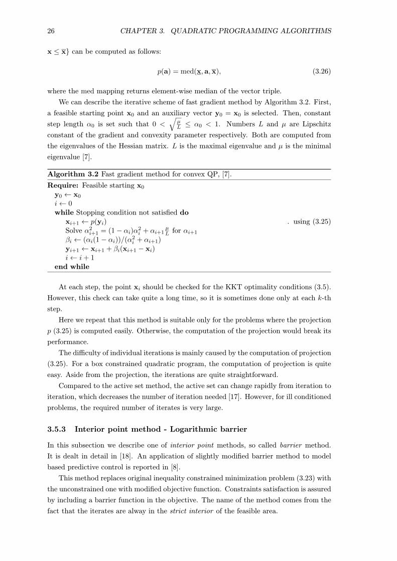
3.5.3 Interior point method - Logarithmic barrier
In this subsection we describe one of interior point methods, so called barrier method.
It is dealt in detail in [18]. An application of slightly modified barrier method to model
based predictive control is reported in [8].
This method replaces original inequality constrained minimization problem (3.23) with
the unconstrained one with modified objective function. Constraints satisfaction is assured
by including a barrier function in the objective. The name of the method comes from the
fact that the iterates are alway in the strict interior of the feasible area.

3.5. INEQUALITY CONSTRAINED QP 27
x1
x2
0 0.5 1 1.5 2 2.5
−0.2
0
0.2
0.4
0.6
0.8
1
1.2
1.4
Figure 3.3: Level lines of the barrier function for a sample two dimensional set.
The new unconstrained problem is solved using e.g. Newton’s method. Obviously, the
solution of the new problem is only an approximation to the original one, because of the
influence of the barrier function.
Barrier function
The barrier function value says how close a point x is to the boundary of the feasible set.
We denote the function ψ and define it as follows.
ψ(x) =m∑i=1
− log(bi − aTi x) for x ∈ Rn satisfying Ax < b. (3.27)
Note that the function grows without bound as x reaches the boundary. This makes the
points outside the feasible set unreachable. The ψ is undefined outside the feasible area
and on the boundary so a strictly feasible starting point is always required.
Level lines of ψ for a sample two dimensional set are plotted in Figure 3.3.
Modified minimization problem is then expressed as
minimize1
2xTGx + fTx + κψ(x), (3.28)
where κ > 0 determines the quality of approximation of function q by q+κψ in the feasible
region. As κ decreases to zero, ψ influences the objective less and less. Hence, the solution
of problem (3.28) gets closer to the solution of the original constrained problem in (3.23).
Sequential decreasing of κ
On one hand, we want number κ to be as small as possible because of the accuracy of
solution, but on the other hand, we want it not to be so small because then it would
be difficult to solve the unconstrained problem. The latter is due to the rapid change of
Hessian near the boundary of the feasible set.

28 CHAPTER 3. QUADRATIC PROGRAMMING ALGORITHMS
Figure 3.4: Sequence of approximate minimizers of (3.28) for decreasing κ.
To overcome this, the minimization is started with some κ. A few iterations of Newton’s
method are done (there is no need for the exact minimizer so an approximate solution
suffices). After that, κ is decreased by a factor ν > 1 and from the previous solution, new
minimization is started.
Parameter ν determines how the objective function in (3.28) differ. If ν is close to
one, the individual problems (3.28) are very similar and so less Newton’s iterations are
required. However, it takes more changes in µ to obtain the same solution. It is a trade-off
and values of 10 to 100 usually work well [18].
We can express the idea by Algorithm 3.3.
Algorithm 3.3 Barrier method for convex QP, [18].
Require: Strictly feasible starting x, κ > 0, νwhile Stopping condition is not satisfied do
Minimize q + κψ starting from x . using e.g. Newton’s methodκ← κ/νx← x?
end while
The iterates of interior point method are quite costly because they involve Newton’s
method. Hence, linear system has to be solved at each step. However, the number of
iterations required to reach the optimum is relatively modest.
Example
In Figure 3.4 a sequence of approximate minimizers x? of (3.28) for different values of κ
is shown. The minimization was started with κ = 10 and it was decreased by the factor
ν = 10 at each step. It can be clearly seen that as κ decreases, the minimizer of q + κψ
gets closer to the one of the original constrained quadratic program (the blue cross).

Chapter 4
Properties of QP algorithms
In this chapter the properties of selected QP algorithms will be shown. We especially treat
the computation time of the algorithms, because it is crucial to the ability to control fast
dynamic processes. Several factors that influence the computation time will be studied via
numerical simulations. We will only study strictly convex quadratic programming algo-
rithms with bound constraints. The number of optimization variables will be sometimes
referred to as QP size throughout the chapter.
The chapter is organized in the following manner. The first section presents the solvers
making use of inequality constrained QP algorithms from Section 3.5. In the second
section, numerical experiments are carried out and the results are discussed. The section
is divided into two subsections. The first of them shows model predictive control example
and the second one randomly generated quadratic programs. The third section summarizes
the results of the experiments.
4.1 QP solvers under test
In this section we briefly present the solvers to be tested in this chapter. Representatives
of each algorithm from the previous chapter were selected. General purpose solvers (quad-
prog, MOSEK) as well as those specific to MPC (qpOASES and FiOrdOs) are described.
4.1.1 quadprog - Active set method
As a part of the Optimization toolbox in Matlab, quadprog represents an ordinary active
set algorithm. It does not have any option to utilize the sequential nature of the QPs arising
in model based predictive control and it is not intended to be used in fast applications. For
more information, please see Matlab help (http://www.mathworks.com/help/optim/ug/
quadprog.html).
4.1.2 qpOASES - Specialized active set method
This solver was specifically designed to fit MPC. It uses so called extended online active
set strategy. It makes use of the fact that the QPs arising in MPC differ in vector f which
is a function of system state. The state space can be partitioned into critical regions much
29

30 CHAPTER 4. PROPERTIES OF QP ALGORITHMS
like in explicit MPC [13]. On the path from the previous state to the current one, the
knowledge about the regions is used to identify the optimal active set faster. It is similar
to warm starting. For further details see [6].
The program is written in C++ with an interface to Matlab. The latest version avail-
able (3.0 beta) was used (minor stability issues were encountered). The source code and
the installation instructions are published on-line at http://www.kuleuven.be/optec/
software/qpOASES.
4.1.3 FiOrdOs - Fast gradient method
Strictly speaking, FiOrdOs is not a solver but a code generator. It generates a C code
to be compiled, and an interface to Matlab. The resulting program solves QPs using
fast gradient method (see [7]). FiOrdOs can be downloaded as a Matlab toolbox from
http://fiordos.ethz.ch. Documentation is available as a part of the toolbox only.
The solver can handle general inequality constraints (Ax ≤ b), but as it calculates the
projection on the feasible set (see Equation (3.25) in the previous chapter), it becomes
very slow. Therefore, we use only simple bound constraints on variables.
4.1.4 MOSEK - Interior point method
MOSEK is an optimization package to solve linear, quadratic, general non-linear and
mixed integer optimization problems. Interfaces to Matlab are included. The QP solver
uses interior point algorithm and is well suited for large scale problems. It is a general
purpose solver and is not intended for fast MPC applications. We include it to compare
MPC specific solvers to the ordinary ones. Documentation can be downloaded on-line at
http://docs.mosek.com/6.0/toolbox.pdf.
Although the package is commercial, academic license is available for research purposes.
For the test, the default options were used.
4.1.5 Fast MPC - Specialized interior point method
This approach originates to [8]. Several modifications to the interior point method (Section
3.5.3) are made in order to decrease the computation time.
Wang and Boyd proposed using a single value of κ and stopping the minimization
after a fixed number of Newton iterations. In addition, they made use of banded structure
of the Hessian matrix (which allowed fast Newton’s step calculation), because they used
different (sparse) MPC formulation. These modifications make their approach very fast.
The resulting solution is only a rough approximation to the exact optimizer but they
shown that the resulting control quality is comparable to the one obtained with exact QP
solution.
Unfortunately, their code (available at http://www.stanford.edu/~boyd/fast_mpc/)
only runs simulations of the regulator problem. It does not allow direct QP solution, so
it cannot be used. The speed however is impressive.

4.2. NUMERICAL EXPERIMENTS 31
We prepared a Matlab substitute interior_point, which implements the algorithm
from the above mentioned paper without exploiting the Hessian structure. However, its
performance is poor compared to the original code or to the other MPC specific solvers.
4.2 Numerical experiments
This section describes two types of numerical experiments. The experiments are chosen to
illustrate typical properties of QP algorithms regarding the computation time. The first
experiment simulates the run of MPC controller while the second one studies the solution
of randomly generated quadratic programs.
All numerical experiments were carried out on a notebook PC with Intel Core 2 Duo
2.1 GHz CPU running 32 bit Ubuntu 10.04 LTS with Linux 2.6.32 kernel. An interface
for quadratic program generation and for solver calling was written in Matlab R2011b.
The source code is attached to this thesis so that one can experiment with MPC and the
solvers.
4.2.1 Computation time measurement
Optimization run-times were measured using tic and toc functions as recommended by
the MathWorks (the producer of Matlab) in [20]. These times do not include the phase 1,
i.e. obtaining a feasible starting point. Additionally, Matlab process was being run with
highest priority so as to decrease the influence of the remaining processes. All the tests
were performed twice and the minimum of the run-times was taken.
4.2.2 Model predictive control example
In order to show the typical features of QP solvers, we will run them in model predictive
controller for a MIMO (multiple input multiple output) dynamic system. The system is
a laboratory model of a helicopter. State space model was identified in [21]. It has two
inputs (main rotor voltage and tail rotor voltage) and two outputs (elevation angle and
azimuth angle).
Both inputs are constrained to be within ±1 V. The outputs are to track desired
reference signals with step changes.
The sampling time is 0.01 s. If it was a real world control, the optimization would
have to be computed by the end of the sample. However, the example is intended just to
show the properties of the solvers, so we do not enforce this time limit anyhow.
Parameters of the controller are np = 100 and nc = 20. Weighting matrices Q = 10I
and R = I. The size (i.e. the number of variables) of resulting QP which has to be solved
at each time step is 2 · nc = 40.
Output reference tracking as well as computed control actions are shown in Figure 4.1.
One can see how the control action hits the limit several times (around 0.2 s, 0.5 s and 1
s) because the reference signal changes rapidly.
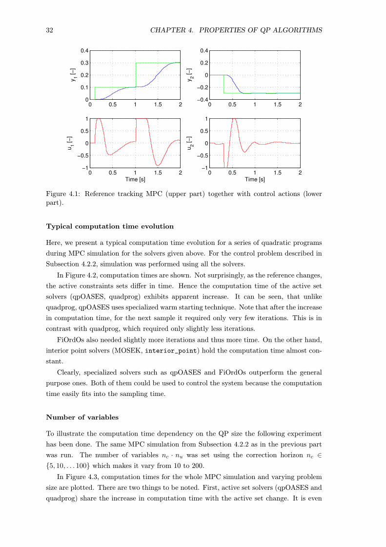
32 CHAPTER 4. PROPERTIES OF QP ALGORITHMS
0 0.5 1 1.5 20
0.1
0.2
0.3
0.4
y1 [
−]
0 0.5 1 1.5 2−0.4
−0.2
0
0.2
0.4
y2 [
−]
0 0.5 1 1.5 2−1
−0.5
0
0.5
1
Time [s]
u1 [
−]
0 0.5 1 1.5 2−1
−0.5
0
0.5
1
Time [s]
u2 [
−]
Figure 4.1: Reference tracking MPC (upper part) together with control actions (lowerpart).
Typical computation time evolution
Here, we present a typical computation time evolution for a series of quadratic programs
during MPC simulation for the solvers given above. For the control problem described in
Subsection 4.2.2, simulation was performed using all the solvers.
In Figure 4.2, computation times are shown. Not surprisingly, as the reference changes,
the active constraints sets differ in time. Hence the computation time of the active set
solvers (qpOASES, quadprog) exhibits apparent increase. It can be seen, that unlike
quadprog, qpOASES uses specialized warm starting technique. Note that after the increase
in computation time, for the next sample it required only very few iterations. This is in
contrast with quadprog, which required only slightly less iterations.
FiOrdOs also needed slightly more iterations and thus more time. On the other hand,
interior point solvers (MOSEK, interior_point) hold the computation time almost con-
stant.
Clearly, specialized solvers such as qpOASES and FiOrdOs outperform the general
purpose ones. Both of them could be used to control the system because the computation
time easily fits into the sampling time.
Number of variables
To illustrate the computation time dependency on the QP size the following experiment
has been done. The same MPC simulation from Subsection 4.2.2 as in the previous part
was run. The number of variables nc · nu was set using the correction horizon nc ∈{5, 10, . . . 100} which makes it vary from 10 to 200.
In Figure 4.3, computation times for the whole MPC simulation and varying problem
size are plotted. There are two things to be noted. First, active set solvers (qpOASES and
quadprog) share the increase in computation time with the active set change. It is even

4.2. NUMERICAL EXPERIMENTS 33
0 50 100 150 20010
−4
10−3
10−2
10−1
100
Simulation step [−]
Co
mp
uta
tio
n t
ime
[s]
quadprog
qpOASES
FiOrdOs
MOSEK
interior_point
Figure 4.2: Typical computation time evolution for MPC simulation. QP size is 40 (see4.2.2) for all the solvers.
more obvious with larger QP size. However, qpOASES is far faster because of its modified
warm staring feature. After the reference change (step number 100 in Figure ??), the
active set it identified and then, the next step is calculated in much less time.
Second, interior point solvers keep the computation time almost constant over the
whole simulation. These are the features of the algorithms that we have already seen in
the previous part (in Figure 4.2).
MOSEK performs well with larger QPs (from the point of view of general optimization
these are small scale ones) but it is rather slow with smaller ones. This is most likely due to
the analysis and modification of the problem that takes place prior to the actual solution
(presolve phase). It takes considerable amount of time which can be neglected when the
number of variables is in the order of hundreds or thousands, but not tens.
Q and R penalty matrices
In this part we review the influence of Q and R matrices on the computation time of
the solvers. MPC simulation for the problem from Subsection 4.2.2 was run. Correction
horizon was set to nc = 20, weighting matrices to R = I and Q = αI with varying
parameter α.
This setting influences the quality of reference tracking as well as the input activity.
The larger is α, the tighter the tracking, but the more aggressive the control.
The effect of large α is illustrated in Figure 4.4. There, solid line shows reference
tracking with parameter α set to 104. Especially note the control action (lower part of
figure) and compare it to the one with α = 10 which is depicted in dashed line.
The computation time median over the whole MPC simulation (200 quadratic pro-
grams) is plotted against varying α for all the solvers in Figure 4.5a. Obviously, fast

34 CHAPTER 4. PROPERTIES OF QP ALGORITHMS
(a) quadprog (b) interior point
(c) qpOASES (d) FiOrdOs
(e) MOSEK
Figure 4.3: Computation time versus QP size.

4.2. NUMERICAL EXPERIMENTS 35
Figure 4.4: Influence of penalty matrix weight on the control quality. Solid line: α = 104,dashed line: α = 10.
gradient method of FiOrdOs performs worse and worse as α increases.
That is because Q and R matrices also influence condition number of QP Hessian
matrix. Condition number of a square matrix is a ratio of its largest singular value to the
smallest. In Figure 4.5b condition number of G is plotted as a function of parameter α.
Evidently, condition number grows with α. In [7] an upper bound on iteration number
is given as a function of condition number and required suboptimality. The number of
iterations grows with condition number and so does the computation time. It is a typical
property of gradient methods.
Active set algorithms also show some increase in the computation time but it is rather
due to the more aggressive control that jumps from one limit to the other (see Figure 4.4)
and makes the active set change rapidly. Therefore, more iterations are needed to reach
the optimum.
Computation times of interior point solvers are almost unaffected by the condition
100
105
10−4
10−2
100
α
Com
puta
tion tim
e m
edia
n [s]
quadprog
qpOASES
FiOrdOs
MOSEK
interior_point
(a) Influence α on the computation time.
100
105
102
104
106
108
α
co
nd
(G)
(b) Influence of α on the condition number.
Figure 4.5: Effect of penalty matrix Q weight α. Note the computation time of FiOrdOsthat is strongly affected by the condition number.
36 CHAPTER 4. PROPERTIES OF QP ALGORITHMS
number.
4.2.3 Random QP
In this Subsection, the properties of QP solvers will be presented on the set of randomly
generated quadratic programs. The first part presents the generation of random QPs. The
second one shows the computation times as a function of the problem size and the number
of active constraints in optimum.
We regard ith constraint as active if aTi x−bi+10−7 ≥ 0. Strict equality is not required
because of possible numerical errors etc.
We exclude interior_point solver from this experiment because even with the toler-
ance set to 10−3, the number of constraints satisfying the above mentioned condition was
different from the one obtained by the rest of solvers. It provides only an approximate so-
lution to quadratic programs. The solution is influenced by the logarithmic barrier which
restricts constraints activation. In other words, the method cannot get right on the con-
straint because there is a nonzero barrier function value (see the level lines of the barrier
function in Figure 3.3).
Active set solver qpOASES was used without its warm starting feature because the
nature of this experiment does not allow it. There is no meaningful sequence of quadratic
programs.
Generation of convex quadratic programs
In order to generate convex quadratic program, we need to get positive semidefinite n by
n Hessian matrix G, column vector f and lower (x) and upper (x) bounds on variables.
Positive definite Hessian matrix G is constructed from its singular value decompo-
sition (SVD). For any symmetric positive definite matrix, its SVD equals its eigenvalue
decomposition [17, A1].
G = USVT︸ ︷︷ ︸SVD
= AEA−1︸ ︷︷ ︸eigenval. d.
= AEAT (4.1)
Here, A is orthogonal (A−1 = AT) and E is diagonal and contains eigenvalues (singular
values) of G.
Orthogonal A is generated from a QR decomposition of random matrix with normally
distributed elements. E is generated as a diagonal matrix with positive elements. These
elements are the eigenvalues of G and they determine the condition number and ensure
positive definiteness.
Vector f is generated as a column vector with normally distributed elements with zero
mean and unit variance.
Bounds on variables (column vectors from Rn) are generated such that the problem
is feasible. That is, the feasible region is non-empty. To do this, we generate random
lower bound vector x with normally distributed elements. Then, we get the upper bound
x = x+c, where c is random positive vector with uniformly distributed elements on (0, k).

4.3. SUMMARY 37
Parameter k, i.e. the width of a band, was being adjusted so that the number of active
constraints spread from 0 to n.
Condition number of Hessian matrix G was set to be in order of 104 to 106. Quadratic
programs were generated with varying number of variables n ∈ (1, . . . , 100). There were
10 · n random quadratic programs for each problem size. This resulted in a set of 50500
QPs.
These problems were solved by the four solvers (excluding interior_point). Mean
computation time was calculated for each QP size and for each number of active con-
straints.
Results
Mean computation times are plotted against quadratic program size and number of active
constraints in the optimum in Figure 4.6.
Overall, quadprog is the slowest. The computation times reach 0.5 s for the larger QP
sizes with many active constraints.
Both active set solvers suffer from increasing computation times for growing number
of active constraints. The computation times required by qpOASES are much longer than
those observed during MPC simulation in Figure 4.3. In this experiment, there is no
sequence of quadratic programs and so no warm starting took place.
Fast gradient method even decreases the time needed with the growing number of active
constraints. This is caused by the projection onto the feasible set. Once the calculated
step points outside the feasible set, it is projected onto it and the corresponding constraints
are activated (see projection formula (3.26)).
With a few active constraints, fast gradient method exhibits typical feature of gradient
methods: slow convergence rate when the problem is not well conditioned [22]. Its behavior
then resembles e.g. the one of gradient method with exact line search seen in Figure 3.1.
Interior point solver MOSEK is unaffected by the number of active constraints in the
optimum.
4.3 Summary
In this chapter, properties of inequality constrained quadratic programming algorithms
were studied. Five solvers using modified algorithms from Section 3.5 were put under test.
Active set methods Active set algorithms need relatively small number of quite de-
manding iterations that include the solution of linear KKT system. It is only possible to
add or remove one constraint from the active set at a time. Hence, when there are many
constraints active in the optimum, many iterations are needed. This was illustrated in
Figure 4.6.
Fast gradient method Computation time of fast gradient method strongly depends
on the condition number. This was shown in Figure 4.5. With a few active constraints,

38 CHAPTER 4. PROPERTIES OF QP ALGORITHMS
(a) quadprog (b) qpOASES
(c) FiOrdOs (d) MOSEK
Figure 4.6: Mean computation time as a function of QP size and number of active con-traints in optimum for random QPs.
this becomes the most apparent as can be seen in Figure 4.6c.
Interior point methods Computation time of interior point algorithm does not depend
on the number of active constraints in optimum. This property was shown in Figure 4.6d.
It has almost no dependence on the condition number as was demonstrated in Figure 4.5.
MOSEK is intended for large scale optimization problems and so it analyzes the prob-
lem prior to the solution which makes it relatively slow with small scale problems (tens
of variables). However, with random QPs and larger scale problems (Figure 4.6d), it
was faster than qpOASES (because it had no sequential advantage here) and faster than
FiOrdOs for small number of active constraints.
MPC specific vs. general purpose solvers Solvers that are specifically designed
for model based predictive control applications, such as qpOASES and FiOrdOS, perform
very well during MPC simulations. General purpose solvers such as quadprog or MOSEK
are not intended for this use and so they are not as good. However, the later one performed
very well. With randomly generated problems it was one of the fastest, except for the
small scale problems, where the analysis of the problem slowed it down (see Figure 4.3e).

Chapter 5
Robustness of unconstrained MPC
In this chapter we discuss the robustness of unconstrained model predictive controller.
For a detailed survey on robust predictive control analysis and design see e.g. [23]. It
is a broad topic to treat so we restrict our scope to the robustness in terms of control
performance.
The chapter is organized as follows. First, the influence of uncertain system parameters
on the closed-loop reference step response is illustrated. A simple second order open-
loop stable system is chosen and its parameters are varied while the predictive controller
remains the same.
Then, the effect of control horizon on robust control performance is discussed. Bench-
mark systems are proposed, and a predictive controller is constructed for each of them.
Then, system parameters are varied in the surroundings of the nominal (exact) model and
their influence on closed loop response is studied. This is done by means of Monte Carlo
simulation.
5.1 Influence of uncertain system parameters
This section illustrates the influence of system-model mismatch caused by incorrect system
parameters. We assume that the structure of a model and a system is the same and so
the mismatch is caused only by the uncertain parameters. The uncertain parameters may
present for example modeling or system identification inaccuracy or the change in the
system under operation.
The mismatch between the model and the system results in prediction mismatch. The
predicted behavior and the real behavior differ and so the controller makes wrong decision.
It leads to poor tracking performance as will be shown below.
In order to avoid this, special measures would have to be taken. The effect of inaccuracy
in the model is similar to the effect of constant disturbance [23]. Therefore, disturbance
estimation can be used to compensate the inaccurate model. Methods such as unknown
input observer are quite common. In [24], the authors included a disturbance model
into state space description and achieved robust offset-free tracking of various classes of
reference signals.
39

40 CHAPTER 5. ROBUSTNESS OF UNCONSTRAINED MPC
However, we did not make any modification to the MPC that was described in Sec-
tion 2.4.
5.1.1 Example
As an example, we present a simple second order SISO system. It is a continuous time
system and we discretize it using zero-order-hold (c2d function in Matlab) with sampling
time Ts such that there is approximately 20 samples per rise time. Then, we treat is as a
discrete time system and design model predictive controller. The transfer function of this
system is as follows:
H(s) =Ke−s·d·Ts
(0.25s+ 1)(as+ 1), (5.1)
where Ts = 0.028 s is sampling time and nominal parameter values are K0 = 1, a0 = 0.1
and d0 = 0. That means open-loop stable system, with zero time delay. Parameter d
determines the length of time delay.
Model predictive controller parameters were set to np = 40, nc = 10, Q = I and R = I.
Prediction horizon length is sufficient to include all important dynamics of the open-loop
step response.
Now, the parameters will be varied and the effect on the closed loop response will
be shown. Closed loop response of nominal system with model predictive controller is
always shown in red coloring. In the literature (e.g. in [25]) the influence of system-model
mismatch is described in more sophisticated ways. Here, only unit step responses are
depicted.
Gain K
In Figure 5.1a, gain K of the system is varied in the range ±20 % around the nominal
value K0. The grey lines show the response with perturbed parameters. Note that the
controller succeeds in offset-free reference tracking only with nominal system. When the
actual parameter is less than nominal, i.e. the controller overestimates the response, closed
loop response is less than required to achieve the reference signal. On the other hand, when
the true parameter is greater than nominal, closed loop response is too high.
Time constant a
Figure 5.1b shows the effect of varying time constant a (a0 plus minus 20 %). Note that
the change in a does not affect DC gain of the system. It seems the same as the effect of
gain, but on a closer inspection, a slight difference appears. The responses in Figure 5.1a
are only scaled up or down, but here, the shapes slightly differ. It is the most obvious
when one compares the largest and the smallest curve. On the largest curve, from sample
20 on, the line is almost straight. On the smallest one, the curve is bent down.

5.2. INFLUENCE OF CONTROL HORIZON 41
Delay d
The effect of input delay not included in the model is shown in Figure 5.1c. Increasing
the delay from 0 to 10 samples causes the closed loop to oscillate. When the delay is
grater than 6 samples, the system becomes unstable. This may be caused by the length of
prediction horizon. According to [26], the prediction horizon should be increased by the
number of delay samples.
(a) Variation in gain K. (b) Variation in time constant a.
(c) Variation in delay d.
Figure 5.1: Step response of nominal (red) and perturbed (grey) system with varyingparameters. The arrows indicate increase in uncertain parameters.
5.2 Influence of control horizon
In this section, the effect of varying control horizon on control performance in presence of
system-model mismatch will be studied. First, mean stage cost, a measure of the quality
of control for a model predictive controller constructed according to Section 2.4 will be
shown. Then, closed loop responses to reference unit step are studied and compared in
terms of mean stage cost during Monte Carlo simulation.
Stage cost C is a sum of squared tracking errors ei and squared control increments ∆ui
weighted by Q and R matrices as in (2.29). Mean stage cost Cm is a cost per simulation
step and it is given by the following formula:
Cm =1
nsC =
1
ns
1
2
(ns∑i=1
eTi Qei +
ns∑i=1
∆uTi R∆ui
), (5.2)

42 CHAPTER 5. ROBUSTNESS OF UNCONSTRAINED MPC
where ns is the number of simulated steps. The only difference between stage cost C and
cost function J in (2.29) is that in the latter one summation happens over predicted errors
and future control increments, in this section, we sum real errors and control increments
applied to the system during the simulation.
5.2.1 Nominal models and controller tuning
All the systems are second order single input single output (SISO) continuous-time systems
with various uncertain parameters. The control objective is to track output reference step
signal.
The systems are discretized with zero-order-hold and then treated as discrete time
systems. Hence, model based predictive controller can be used. The sampling time is set
is set such that it covers the dynamics well.
These systems represent typical simplified models of various processes.
System A: Two real poles + gain
Continuous time transfer function is given as follows:
H(s) =K
(0.25s+ 1)(as+ 1), (5.3)
where nominal parameter values are K0 = 1 and a0 = 0.1. Sampling time is 0.028 s. Step
response of the discretized system is plotted in Figure 5.2a.
System B: Integrator
H(s) =K
s(as+ 1)(5.4)
There are two uncertain parameters with nominal values K0 = 1 and a0 = 0.25. Sampling
time was set to 0.05 s. Step response of the discretized system is plotted in Figure 5.2b.
System C: Two real poles + unstable zero
This system has an unstable zero. Transfer function is given as follows:
H(s) =K(bs− 1)
(0.25s+ 1)(as+ 1), (5.5)
with nominal parameter values K0 = 1, a0 = 0.1 and b0 = 0.5. Sampling time for this
system is 0.014 s. Step response of the discretized system is plotted in Figure 5.2c.
System D: Transport delay
This system includes input transport delay.
H(s) =e−s·d·TsK
(0.25s+ 1)(as+ 1), (5.6)

5.2. INFLUENCE OF CONTROL HORIZON 43
0 0.5 1 1.5 2 2.50
0.2
0.4
0.6
0.8
Time [s]
y [−
]
(a) System A
0 1 2 3 4 50
2
4
Time [s]
y [−
]
(b) System B
0 0.2 0.4 0.6 0.8 1 1.2 1.4−0.2
0
0.2
0.4
0.6
0.8
y [−
]
(c) System C
0 0.5 1 1.5 2 2.50
0.2
0.4
0.6
0.8
Time [s]
y [−
]
(d) System D
Figure 5.2: Step responses of the nominal models.
with nominal parameters K0 = 1, a0 = 0.1 and d0 = 0. Note that in the nominal model,
there is no delay. It is rather put into the system to be controlled, which causes the effect
that was shown in Figure 5.1c. Sampling time is the same as the one for system A, that
is Ts = 0.028 s. Step response of the discretized system is plotted in Figure 5.2d.
Controller tuning
Model predictive controller was set up by trial and error such that it ensured reasonably
good reference tracking with the nominal system. Prediction horizon was always set to
np = 40. This is sufficient to include all important dynamics and steady state of the
open-loop step response (impulse response in case of system B). Weighting matrices are
identity matrices of appropriate size: tracking error penalty Q = 100I (10I for system D)
and control increment penalty R = I.
5.2.2 Monte Carlo simulation
The parameters are set with uniform distribution at the interval±20 % around the nominal
value. The only exception to this rule is the delay in 5.2.1, which was generated from the
set {0, 1, 2, 3}. All the parameters were changed simultaneously.
The control horizon nc was successively set to 1, 2, 5 and 10 samples respectively. For
each nc there were 500 simulation runs with all the systems from the previous subsection.
With all the data collected, mean stage cost Cm from (5.2) was evaluated. Then the
histograms of mean stage cost were plotted. The results are discussed bellow.
System A
The resulting histogram is shown in Figure 5.3a. Notice a red vertical line that shows
mean stage cost for the nominal system. Obviously, as we increase the control horizon
from one to two samples, nominal mean stage cost decreases. The decrease at the change
from two to five or from five to ten is not that significant. This is a well known behavior
and it is described e.g. in [1].

44 CHAPTER 5. ROBUSTNESS OF UNCONSTRAINED MPC
0 0.5 1 1.5 2 2.5 30
50
100
150n
c = 1
0 0.5 1 1.5 2 2.5 30
50
100
150n
c = 2
0 0.5 1 1.5 2 2.5 30
50
100
150n
c = 5
0 0.5 1 1.5 2 2.5 30
50
100
150n
c = 10
Mean stage cost [−]
(a) System A
0 1 2 3 4 5 60
50
100
150n
c = 1
0 1 2 3 4 5 60
50
100
150n
c = 2
0 1 2 3 4 5 60
50
100
150n
c = 5
0 1 2 3 4 5 60
50
100
150n
c = 10
Mean stage cost [−]
(b) System B
Figure 5.3: Histogram of mean stage cost. Red line shows cost with nominal system.
System B
The results are shown in Figure 5.3b. There is significant decrease in mean stage cost
when the control horizon is set to 2 instead of 1.
System C
The results for the system with an unstable zero are plotted in Figure 5.4a. The increase
in control quality is much almost insignificant when nc increases from 1 to 2. It is in
contrast with systems A and B. This is true even for the nominal system. This is caused
by the fact that the tracking error is dominated by the negative response coming from
the unstable zero. The range of costs remains roughly the same for all the control horizon
lengths.
System D
For this system, different weighting matrix Q = 10I was used. The reason for this is that
with Q = 100I the system became unstable even with one sample delay.
The results for system D are plotted in Figure 5.4b. Nominal system’s cost exhibits
similar decrease with growing control horizon. However, for control horizon five and ten the
oscillation (illustrated in Figure 5.2d) became more intensive. Hence, the cost exceeded 0.4.
This suggests that the controller might be slightly less robust to system-model mismatch
when an unmodelled input delay is present and nc is relatively large.
Summary
The effect of increased control horizon on the control quality is quite apparent for all
the systems except the one with unstable zero. This is probably due to the negative
response coming from the transfer function zero. Control horizon set to one gave the

5.2. INFLUENCE OF CONTROL HORIZON 45
0 2 4 6 8 100
50n
c = 1
0 2 4 6 8 100
50n
c = 2
0 2 4 6 8 100
50n
c = 5
0 2 4 6 8 100
50n
c = 10
Mean stage cost [−]
(a) System C
0 0.2 0.4 0.6 0.8 10
50
100n
c = 1
0 0.2 0.4 0.6 0.8 10
50
100n
c = 2
0 0.2 0.4 0.6 0.8 10
50
100n
c = 5
0 0.2 0.4 0.6 0.8 10
50
100n
c = 10
Mean stage cost [−]
(b) System D
Figure 5.4: Histogram of mean stage cost. Red line shows cost with nominal system.
worst performance. The larger control horizon settings (2, 5 and 10) provided better
control in terms of mean stage cost.
Any improvements to robustness in terms of control quality were not observed. The
range of mean stage cost remained approximately the same for all the systems.

46 CHAPTER 5. ROBUSTNESS OF UNCONSTRAINED MPC

Chapter 6
Conclusion
In the first chapter, we presented the basic idea behind model based predictive control,
briefly reviewed history of MPC and finally, the state of the art was shown.
In the second chapter, the most important components of predictive controller were de-
scribed. Receding horizon concept was presented and simple constraints were illustrated.
Then, elementary implementations of the regulator problem, the reference tracking prob-
lem and offset-free tracking were shown. It was also shown that the optimization problem
arising in MPC is a quadratic program.
The third chapter dealt with quadratic programming, which is a minimization of
quadratic function. First, quadratic program was defined, and conditions for it to be
convex were stated. Then, quadratic programs were divided into three groups according
to the type of constraints and several algorithms to solve each of them were presented.
For the unconstrained quadratic programs, two gradient methods and Newton’s method
were presented. Equality constrained QPs can be solved through the solution of the KKT
system. Finally, active set method, fast gradient method and interior point method for
the solution of inequality constrained quadratic programs were shown.
The fourth chapter addressed the first part of the assignment, i.e. the properties of QP
algorithms and computation time distribution. In order to do this, several solvers repre-
senting each algorithm class were selected. Then, a simple benchmark control problem was
chosen to deploy MPC controller and to run the simulation with the examined solvers.
Finally, the solvers were tested with randomly generated bound constrained quadratic
programs.
The influence of optimization problem size, condition number and the number of active
constraints in optimum on the computation time was illustrated. The following relations
were observed during the experiments.
The computation time is highly affected by the number of variables. Active set method
exhibits quite strong dependence of computation time on the number of active constraints
in the optimum. Computation time of fast gradient method strongly depends on the
condition number and for ill-conditioned problems it depends on the number of active
constraints as well. The larger the condition number, the slower the rate of convergence.
Interior point method keeps the computation time almost constant irrespectively of the
number of active constraints and condition number.
47

48 CHAPTER 6. CONCLUSION
The fifth chapter addressed the second part of the assignment. The chapter presented
the robustness of unconstrained MPC controller in terms of control performance. First,
the influence of individual model parameters inaccuracy was shown. Then, the effect of
MPC control horizon length on the control quality was studied.
It was demonstrated that there is a need for an exact model of a system. In case
of system-model mismatch, the control quality is poor, unless special care is taken such
as disturbance estimation through an observer. For all the systems, no improvement to
robustness was observed with increasing control horizon.
Generally, it is a good idea to set control horizon long enough. For the simple second
order systems from Section 5.2, control horizon set to two gave almost the same control
performance as five and ten did. This is good to know, because the shorter control horizon
dramatically decreases optimization problem complexity. However, control horizon set to
one gave much worse control performance.
The only difference was the system with unstable zero. The control performance was
roughly the same for all the control horizon settings. This is probably due to the fact that
the tracking error was dominated by the negative response caused by the zero. Surprisingly,
for a system with unmodelled time delay, longer control horizon may lead to poor tracking
because the system oscillates.
Both tasks given in the assignment were accomplished. However, there are still many
open questions to deal with. Here, only two of them are pointed out. First, there are
many more QP algorithms to study. Several approaches that combine the properties of
the algorithms dealt in this thesis exist that give great performance in MPC. Second,
different cost functions can be used in MPC, which leads to different optimization tasks
and therefore to different approaches to the solution.

Bibliography
[1] J. A. Rossiter, Model-based predicitve control: a practical approach. CRC Press LLC,
2003.
[2] J. Richalet, A. Rault, and J. Testud, “Algorithmic control of industrial processes,”
in Proceedings of the 4th IFAC symposium on identification and system parameter
estimation, pp. 1119–1167, 1976.
[3] C. R. Cutler and B. L. Ramaker, “Dynamic matrix control - a computer control
algorithm,” in Proceedings of the joint automatic control conference, 1980.
[4] J. Rawlings, “Tutorial overview of model predictive control,” Control Systems, IEEE,
2000.
[5] S. J. Qin and T. A. Badgwell, “A survey of industrial model predictive control tech-
nology,” vol. 11, pp. 733–764, 2003.
[6] H. J. Ferreau, P. Ortner, P. Langthaler, L. D. Re, and M. Diehl, “Predictive control
of a real-world Diesel engine using an extended online active set strategy,” Annual
Reviews in Control, vol. 31, pp. 293–301, Jan. 2007.
[7] S. Richter, C. N. Jones, and M. Morari, “Real-time input-constrained MPC using fast
gradient methods,” Proceedings of the 48h IEEE Conference on Decision and Control
(CDC) held jointly with 2009 28th Chinese Control Conference, pp. 7387–7393, Dec.
2009.
[8] Y. Wang and S. Boyd, “Fast Model Predictive Control Using Online Optimization,”
IEEE Transactions on Control Systems Technology, vol. 18, pp. 267–278, Mar. 2010.
[9] S. Richter, S. Mariethoz, and M. Morari, “High-speed online MPC based on a fast
gradient method applied to power converter control,” in American Control Conference
(ACC), 2010, pp. 4737–4743, 2010.
[10] K. Basterretxea and K. Benkrid, “Embedded high-speed Model Predictive Controller
on a FPGA,” 2011 NASA/ESA Conference on Adaptive Hardware and Systems
(AHS), pp. 327–335, June 2011.
[11] F. Borrelli, A. Bemporad, and M. Morari, “Predictive Control for linear and hybrid
systems,” 2011.
49

50 BIBLIOGRAPHY
[12] G. Valencia-Palomo, M. Pelegrinis, J. A. Rossiter, and R. Gondhalekar, “A move-
blocking strategy to improve tracking in predictive control,” American Control . . . ,
pp. 6293–6298, 2010.
[13] A. Bemporad, M. Morari, V. Dua, and E. N. Pistikopoulos, “The explicit linear
quadratic regulator for constrained systems,” Automatica, vol. 38, pp. 3–20, Jan.
2002.
[14] O. Šantin, Influence of Model Uncertainty on Constraints Handling in Predictive
Control. Diploma thesis, CTU in Prague, 2009.
[15] G. Franklin, J. D. Powell, and A. Emami-Naeini, Feedback control of dynamic systems.
Pearson, 2010.
[16] B. Grünbaum, Convex polytopes. New York: Springer, 2nd ed., 2003.
[17] J. Nocedal and S. J. Wright, Numerical Optimization. New York: Springer, sec-
ond ed., 2006.
[18] S. Boyd and L. Vandenberghe, Convex Optimization. Cambridge University Press,
seventh ed., 2004.
[19] Y. Nesterov, Introductory Lectures on Convex Optimization: A basic Course. Kluwer
Academic Publishers, 2004.
[20] M. Knapp-Cordes and B. McKeeman, “Improvements to tic and toc Functions for
Measuring Absolute Elapsed Time Performance in MATLAB,” MATLAB Digest,
pp. 1–4, 2011.
[21] M. Hoč, Helicopter in virtual space. Diploma thesis, CTU in Prague, 2008.
[22] D. P. Bertsekas, “On the Goldstein - Levitin - Polyak Gradient Projection Method,”
IEEE Transactions on Automatic Control, vol. AC-21, no. 2, pp. 174–183, 1976.
[23] A. Bemporad and M. Morari, “Robust model predictive control: A survey,” Robust-
ness in identification and control, 1999.
[24] U. Maeder and M. Morari, “Offset-free reference tracking with model predictive con-
trol,” Automatica, vol. 46, pp. 1469–1476, Sept. 2010.
[25] A. S. Badwe, R. S. Patwardhan, S. L. Shah, S. C. Patwardhan, and R. D. Gudi,
“Quantifying the impact of model-plant mismatch on controller performance,” Jour-
nal of Process Control, vol. 20, pp. 408–425, Apr. 2010.
[26] J. L. Garriga, M. Soroush, and H. M. Soroush, “On the Effects of Tunable Parameters
of Model Predictive Control on the Locations of Closed-Loop Eigenvalues,” Industrial
& Engineering Chemistry Research, vol. 49, pp. 7951–7956, Sept. 2010.

Appendix A
Contents of the attached CD
The attached CD contains two directories:
thesis: Full text of the thesis in Portable Document File.
program: Source codes for MPC controller simulation and QP algorithms from Chap-
ter 3. Several examples of MPC simulation and QP solution are included as well.
Matlab installation is required.
51
Recommended


![ALGORITMY TEORIE C ISEL - Masaryk Universitykucera/texty/ATC2014.pdf · 2014. 6. 29. · 1 ALGORITMY 1 ALGORITMY TEORIE C ISEL Radan Ku cera verze 29. cervna 2014 Literatura [Ca]](https://img.pdfslide.us/doc/110x75/60d8964dfd9cc636797ddcec/algoritmy-teorie-c-isel-masaryk-kuceratextyatc2014pdf-2014-6-29-1-algoritmy.jpg)


![Index [downloads.diablaoutdoor.com]4.5 _Index Trip_04 Ploid_12 Mareta_18 Sail mini_22 Abstrakt Mona_26 Lena_30 Spaces Diabla_34 Technical section_38](https://img.pdfslide.us/doc/110x75/5f3f1666d44bc3457e5294b4/index-45-index-trip04-ploid12-mareta18-sail-mini22-abstrakt-mona26-lena30.jpg)