Putting the Hobson-Rogers model to the test
A. Platania1 and L. C. G. Rogers2
July 2003
Abstract
In this paper, we take the model of Hobson & Rogers (1998) for the movement of an asset,and we fit it to data. The model of Hobson & Rogers is a stochastic volatility model, wherethe volatility depends on the offset of the current log-price from its exponentially-weightedhistorical value. As such, the model is complete, and there are unique preference-independentprices. In the datasets we study, there is very clear evidence that the volatility does indeedvary with offset; we use PDE methods, and simulation methods, to fit the model to data,and find that the fit is generally better than the Heston model.
1Facolta di Scienze Statistiche ed Economiche, Via Cesare Battisti 241, 35121 Padova, Italy2Statistical Laboratory, Wilberforce Road, Cambridge CB3 0WB, GB; email =
Introduction
The striking work of (BLACK and SCHOLES 1973) and the simultaneous opening of
the Chicago Board Option Exchange in 1973 started a new era for financial mathe-
matics. The Black-Scholes formula is still widely used among traders to price vanilla
options, at least as a metric for the risk implied by actual quotes. However, espe-
cially after the market crash of 1987 and the advent of powerful computers and new
mathematical technologies, many efforts have been devoted to develop new models
and to study their pricing implications.
As a matter of fact, volatility of the underlying stock is not constant (see e.g.
(BLATTBERG and GONEDES 1974)), and implied volatility varies across strikes.
In a famous paper (RUBINSTEIN 1985) proved that short maturity out of the money
calls are priced higher relative to other calls than Black and Scholes would predict,
and that strike price biases are statistically significant and can reverse over time.
The specification of volatility as a stochastic process is extremely natural, since
it can explain a number of different empirical findings, such as distributional proper-
ties of the underlying or the presence of transaction costs. For example the observed
correlation between volatility and asset prices can be explained by ‘level dependent’
volatility models like the Constant Elasticity of Variance (CEV)3 model of (COX
and ROSS 1976). Stochastic volatility can also arise endogenously: (PLATEN and
SCHWEIZER 1998) obtain it through an equilibrium argument, modelling the be-
haviour of market participants.
Fully stochastic volatility models (introduced in 1987 by (HULL and WHITE
1987), (SCOTT 1987), and (WIGGINS 1987)) are again motivated by the idea that
a sensible specification of the volatility process can offer generality and analytical
tractability. Sadly it is often the case that using ‘plausible’ parameters, like the
negative correlation between volatility and prices observed in practice, it is difficult
to match actual option prices. In their empirical study (BAKSHI, CAO, and CHEN
3Although widely used as an alternative to the standard log-Brownian model, it is not hard to see that if the
exponent is less than 1 then the CEV stock price will hit zero in finite time almost surely; in some applications
it may be hard to justify this property.
2
1997) find indeed that structural parameters obtained via calibration are significantly
different from their historical time-series estimated counterparts.
In this sense the fact that the literature is increasingly concerned with the con-
sistency of models both cross-sectionally and intertemporally is not surprising. The
study in Section 2 is intended to support the volatility structure of our model before
the investigation of its option pricing implications.
Generalized Autoregressive Conditional Heteroskedastic (GARCH) processes are
in a limit sense the discrete time counterpart of stochastic volatility models (see
(CORRADI 2000)). Under assumptions on the utility of the investor, (DUAN 1995)
derives unique option prices. Nonetheless without the familiar (complete) continuous
time framework it is impossible to define an exact replicating strategy.
Usually, a pricing model has to balance theoretical generality and consistency of
the volatility structure against the ability to estimate its parameters efficiently and
precisely. In the first sense the literature achieved some encouraging results, raising
new important issues and developing different approaches (see (BATES 2003) and
(GHYSELS, HARVEY, and RENAULT 1996) for an insightful review). Recently
(FOUQUE, PAPANICOLAU, and SIRCAR 2000) proposed an efficient and robust
(almost specification free) method for the modeling, analysis and stable estimation
of important groupings of market parameters, exploiting the fast mean reversion of
volatility. Their key idea is to compute a simple correction of Black-Scholes model
which reflects the effect of stochastic volatility on derivative prices.
The paper is organized as follows: in Section 1 we present the model, underlying
the particular case used in the numerical procedures. In Section 2 we propose a
simple empirical analysis to support our main modelling assumption. In Section 3
we explain both the finite difference and the Monte Carlo methods used to calibrate
the model. In Section 4 we perform a limited but instructive comparison between
some well known pricing models. In Section 5 we discuss the use of asymptotic
expansion for our model. Finally in Section 6 we conclude the paper and we suggest
some remaining research issues.
3
1 The Hobson-Rogers model
(HOBSON and ROGERS 1998) (henceforth HR) specify local volatility in terms of
weighted moments of past returns. Let us denote with Zt = log(e−rtPt) the log-
discounted price process, and define the offset function of order m as
S(m)t = λ
∫
∞
0e−λu(Zt − Zt−u)mdu, (1)
where the parameter λ describes the weight of historic observations. Stock prices
are driven by the stochastic differential equation
dZt = σ(
t, Zt, S(1)t , . . . , S
(n)t
)
dBt + µ(
t, Zt, S(1)t , . . . , S
(n)t
)
dt
for some smooth functions σ(·) > 0 and µ(·).Since σ(·) can eventually depend on Pt, the model includes as a subclass the case
when the volatility rate is a deterministic function of the underlying. Furthermore
the hypotheses preserve completeness, allowing for preference independent option
pricing. This last feature constitutes an advantage over fully stochastic volatility
processes, where arbitrage considerations are not sufficient to identify ‘risk premia’
uniquely.
In the following, we will assume the instantaneous volatility is a function of the
first order offset St = S(1)T only, since we want to obtain a tractable PDE and to
solve it with reliable precision. HR showed that even in this case the model has
the potential to explain volatility smiles and skews, and our simulation studies seem
to suggest that including higher order offset functions does not improve the results
significantly.
Using equation (1) we readily decompose St as the deviation of the current price
from an exponentially weighted average of past records
St = Zt − λ
∫
∞
0e−λuZt−udu. (2)
The latter says that λ determines the horizon of the ‘moving time window’ of the
integral on the right. For bigger values of this parameter, St is more dependent on
the recent past, while small values almost identify the offset increments with price
4
changes. Obviously in this case a level dependent volatility assumption would be
numerically more convenient.
To build the basic model used in the numerical procedures, consider the risk
neutral measure P and the P-Brownian motion Bt. Let e−rtPt be a P-martingale
solving dPt = σPtdBt, so that by Ito’s formula
dZt = σdBt −1
2σ2dt. (3)
With the substitution u = t − s equation (2) gives
St = Zt − λe−λt
∫ t
−∞
eλsZsds,
and we can easily compute the differential of St
dSt = dZt − λStdt. (4)
HR find a general formula for the differential of higher order offsets and prove that(
Zt, S(1)t , . . . , S
(n)t
)
forms a Markov process.
Finally take U = Z − S and denote with f(t, Ut, Zt) the price at time t < T of a
contingent claim worth
f(T,UT , ZT ) = q(ZT ) (5)
at maturity T . Using standard arguments we derive HR PDE
0 = ft + λ(Z − U)fU − 1
2σ(Z − U)2(fZZ − fZ), (6)
with boundary condition (5).
2 Does volatility depend on the offset?
Volatility changes over time: the explanation of its movements represent a key issue
in finance theory, and various modelling attempts have been proposed in literature
(see for instance (SCHWERT 1989)).
The dependence between volatility and past returns is intuitively appealing. In
their conclusions (DUMAS, FLEMING, and WHALEY 1998) suggest to relate the
volatility surface to past changes in the index level, while pratictioners commonly
5
use exponentially weighted moving averages to forecast volatility. Moreover, this
hypothesis introduces an effect of volatility clustering. It is in fact clear from Equa-
tion (1) that, depending on the values of λ, large changes in the price will cause
the offset to substantially modify for a certain period. Many other characteristics
of the volatility dynamics are naturally explained, including the local persistence
and state dependent volatility of volatility recently observed by (CHERNOV, GAL-
LANT, GHYSELS, and TAUCHEN 2003).
We carry out a simple analysis using SP500 index settlement prices collected
from the CME, with sample period between Jan 1993 and Dec 2002. Consider the
approximation for the offset process S given by
St =
M∑
i=0
wi
W(Zt − Zt−i), (7)
where the weights are wi = e−λi∆t and W is their sum. As a corresponding estimate
of volatility take
σt =
√
√
√
√k
M∑
i=1
wi
W(Zt−i+1 − Zt−i − µt)2, (8)
where µt is the weighted mean of log returns between time t − M and time t, and
k = W 2/∑
(
W 2
M − w2i
)
is a correction to make σ2t unbiased. All estimates are
computed on a daily basis, and we consider a calendar of 242 trading days implying
a unit of time ∆ = 1/242.
We fixed the lookback as M = 2000 using overlapping data4, that is we dynam-
ically compute an estimate based on 2000 historical observations for each trading
day. Note that thanks to their particular construction (7) and (8) are based on the
same amount of past information.
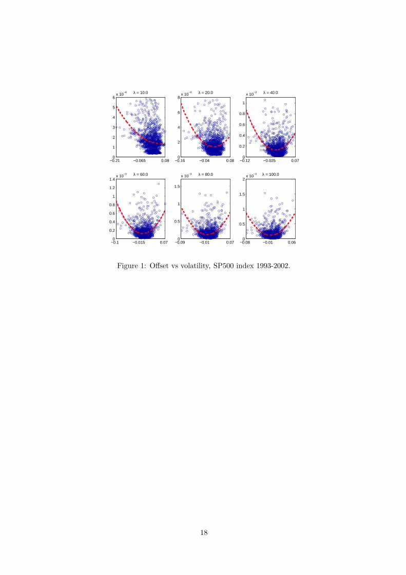
[ Figure 1 about here ]
The six plots in Figure 1 show the relationship between our estimate (7) of the
offset and (8) of the volatility for various values of λ. Each subplot includes the
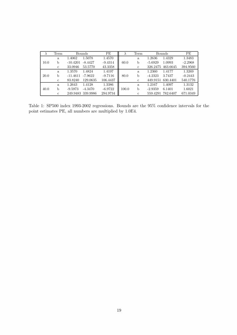
curve obtained regressing the volatility σt over a second order polynomial in the
offset a + bS + cS2. The resulting minimum squared error parameters are reported
4This huge M is to ensure that both St and σt are computed with a sufficient number of data even in the case
where λ is small.
6

in Table 1, together with their 95% confidence intervals and the corresponding λ
values.
[ Table 1 about here ]
Nonetheless a simple parabola is unlikely to capture the relation between offset
and volatility. Extensive numerical studies prove that a very effective specification
for the volatility function is given by
σ(s) =1 + as + bs2
c + ds + es2, (9)
combining the flexibility of rational polynomials with a reasonable number of pa-
rameters. The alternative
σ(s) =√
a + bs2 ∧ N , (10)
originally proposed in HR and discussed in Section 4, turned out to be particularly
effective because it largely reduced efforts involved in the optimization problem.
This qualitative study provides empirical evidence in favour of our conjectures
and help us in the selection of a proper volatility function.
3 Empirical Methodology
The parameters of HR models can be estimated using different strategies. The
likelihood function cannot be computed, but calibration could be based on statisti-
cally respectable procedures thanks to the developements of econometric literature
during the last decade. (ANDERSEN, CHUNG, and RENSEN 1999) make an exten-
sive investigation of the EMM technique and provide a source of related literature.
(TOMPKINS 2001) applies a similar method to estimate the parameters of a class
of Heston related models, and finds that the inclusion of a stochastic volatility pro-
cess consistent with the objective process alone does not explain volatility smiles.
(CHERNOV, GALLANT, GHYSELS, and TAUCHEN 2003) compare many diverse
specifications on a long daily Dow Jones industrial average index return series and
suggest that the choice between models should be based upon practical criteria.
These approaches benefit from the existence of a proper statistical theory, but
some drawbacks remain. The choice of the score generator or of the key attributes is
7

often critical and influences the precision in terms of standard errors. The presence
of local optima, common to every optimization problem, has to be tackled when
maximizing the quasi-likelihood. Moreover, (ROGERS and SATCHELL 2000) show
why linking distributional properties of real world and risk neutral measures should
be considered carefully.
Calibration has been widely considered in the literature. (SCOTT 1987) uses
Monte Carlo simulation to estimate his stochastic volatility model, optimizing over
the sum of squared errors between the model and actual prices. He finds that his
model outperforms Black and Scholes, but tends to overprice out of the money op-
tions, and he suggests to use a larger sample. The so called ‘indirect inference’
techniques obtained varying success. (JACKWERTH and RUBINSTEIN 1996) de-
rive underlying asset risk neutral probability distributions implied by index option
and underlying asset prices. Their results show robustness over alternative optimiza-
tion specifications and stability of implied levels of skewness and kurtosis over time.
Furthermore they outperform Black and Scholes lognormality assumption in the ex-
planation of rare events. More recently (DUMAS, FLEMING, and WHALEY 1998)
calibrate a model with deterministic volatility function and find that its predictive
performance is no better than ad-hoc smoothings of Black and Scholes.
We used two different approaches to calibrate our model. The solution of PDE
(6) is supposed to be fast and accurate when it converges, but the idea of simulating
SDEs (3) and (4) is also attractive since the model is driven by one single source of
uncertainty.
3.1 Finite difference methods
The application of finite difference methods to option pricing goes back at least to
(SCHWARTZ 1977) and (BRENNAN and SCHWARTZ 1978), and later (COURTADON
1982) and (HULL and WHITE 1990). A recent textbook treatment of the subject
is given by (TAVELLA and RANDALL 2000).
The main idea of finite difference methods is to convert a PDE into a set of
difference equations and to solve them iteratively.
In order to obtain a numerical solution of the PDE (6) by finite differencing we
8
need first of all to build a grid containing a discrete set of points for each variable.
We determined the range for the logprice and the offset according to the laws of the
solutions of the corresponding SDEs, thus linking the grid size to the parameters
used for each solution. Then we fixed a reasonable number of steps in each direction
testing our results in the Black and Scholes and other known settings.
More advanced techniques use combinations of explicit and implicit finite differ-
ence methods. While the hopscotch method alternates between them, the θ-method
uses a weighted combination of explicit and implicit approximations. The typical
final system has the form
A(θ)fi = B(θ)fi+1, i = 0, . . . , T − ∆t, (11)
where A and B are typically huge sparse matrices depending on both the weight θ
and the problem’s parameters. We choose the well known Crank-Nicholson method,
that uses the uniform weight θ = 12 . This scheme is stable and high-order accurate.
As with any implicit method, the linear system (11) has to be built and solved. In
this task it is essential to take full advantage of the structure of the matrices A and
B, using routines for sparse linear systems such as the freely distributed UMFPACK
4.0 in order to avoid the direct computation of A’s inverse.
Another important problem is how to compute the value of the derivatives on
those points where we are forced to cut the range of our variables for computational
needs; in other words we must provide some numerical boundaries for the edges of
our finite grid.
Various easy approaches are possible, such as forcing the exercise of the derivative,
or killing or reflecting the diffusion outside the edges. Unfortunately, this is not
sufficiently precise especially in a two dimensional scenario.
The undetermined coefficient method approximates the value of a partial derivatives
at a point using a weighted sum of the solution values on the nearest grid points, for
example
fz(t, St, Zt) = af(t, St, Zt + ∆Z) + bf(t, St, Zt + 2∆Z) + cf(t, St, Zt + 3∆Z),
where fz(·) is the partial derivative of f with respect to Z and ∆Z is the Z increment
for our grid. We can now expand f(·) in Taylor series and match the two sides of
9

the equation, determining the unknown coefficients through a linear system. This is
more difficult for the mixed derivative fsz(·), where we used a multivariate Taylor
expansion with fifteen terms (and coefficients to determine): in this case we used
some software to manipulate symbolic algebra.
3.2 Monte Carlo simulations
Since their first appearance in (BOYLE 1977), Monte Carlo techniques proved to be a
very flexible tool in financial applications. (BOYLE, BROADIE, and GLASSERMAN
1997) discuss some of them and describe a number of useful variance reduction tech-
niques studying their efficiency. For complete and detailed references, see (KLOEDEN
and PLATEN 1999) and (GLASSERMAN 2003).
The price of a derivative security is the expected value under the risk neutral
P of its discounted payoff. The Monte Carlo method lends itself naturally to this
evaluation. The main principle is to generate sample paths of the underlying assets
over the time interval of interest, compute the discounted payoff of the derivative
according to its definition and take the average over the sample paths. By the strong
law of large numbers this estimate converges to the true price, and we easily obtain
an estimate of its error from the central limit theorem.
In order to obtain a remarkable precision we used Richardson extrapolation, Mil-
stein’s method to improve the strong order of convergence, the antithetic variable
technique and the control variate technique, using Black and Scholes price as a con-
trol variate.
Monte Carlo techniques are not very precise for calibration, for example changing
the initial random seed prices can vary significantly. Nonetheless thanks to this ap-
proach we were able to answer a number of questions. First of all, we realized that in
the data sets we considered higher order offset inclusion is not needed. Furthermore
Monte Carlo prices provide a rough comparison to PDE prices, and the simulated
paths help to fix the size of the finite difference schemes grids. In the following, all
reported prices are obtained via finite differencing.
10

3.3 Cost function specification
The objective to be minimized was the sum over the different strikes of the relative
errors. We do this because it represents a measure of the success of an investment.
Formally, let θ be the vector of parameters of the volatility function (9) together
with λ, and denote by Θ its parametric space. Let fHR(t,Ki, Zt, St, θ) be the HR
price when the strike is Ki for i = 1, 2, . . . , N and the estimate St is computed via
(7), and let v(t,Ki, Zt) be the actual price. We want to find
minθ ∈ Θ
N∑
i=1
|v(t,Ki, Zt) − fHR(t,Ki, Zt, St, θ)|v(t,Ki, Zt)
,
or the minimum of the logarithm of the sum when we expect some percentage errors
to be particularly big. We used many different routines to solve this global optimiza-
tion problem, but we obtained the best results with CFSQP, a set of C functions
based on Sequential Quadratic Programming. Actually, each evaluation of the cost
function takes about 0.1 seconds on a PENTIUM 3.6 Ghz Linux machine both for
the finite difference and the Monte Carlo approaches, while the whole optimization
needs between one and five minutes.
4 Comparisons with different models
Testing alternative models is a challenging task, requiring careful procedural choices
to build a reliable empirical methodology. The purpose of the present section is to
gain a rough idea of the empirical performances of some well known pricing models
in the limited scenario of a cross-section of option prices. Let us briefly introduce
the proposed alternatives.
Constant Elasticity of Variance The CEV model defines volatility as a deter-
ministic function of the stock price, trying to capture the leverage effect observed by
(BLACK 1976). The stock price follows the diffusion
dPt = µPtdt + δPβ/2t dBt,
so that for β < 2 the volatility σ(St, t) = δP(β−2)/2t is inversely related with prices,
while if β = 2 we recover the Black and Scholes case.
11
(SCHRODER 1989) expresses the CEV pricing formula in simple terms of the non-
central chi-square distribution5, and the optimization over the two parameters re-
quires little effort too.
Heston model In (HESTON 1993) model the spot asset is assumed to be governed
by the diffusion
dPt = µPtdt + σtPtdB(1)t
and the volatility is an Ornstein-Uhlenbeck process. This can be written as the
square-root process
dνt = κ (φ − νt) dt + ςσtdB(2)t ,
where νt = σ2t . The model allows correlation ρ between B
(1)t and B
(2)t , and it is
possible to obtain a close form solution for vanilla options via Fourier inversion (see
(DUFFIE 2001) for a detailed exposition of the transform analysis approach). This
involves just the computation of a non trivial integral, but a further assumption that
gives the price of volatility risk has to be made to price contingent claims.
We performed the optimization over six parameters: λ specifies the risk premium,
κ∗ = κ+λ the mean reversion, φ∗ = κφ/(κ+λ) the long run variance, ν0 the starting
(current) variance, ρ the correlation and ς the volatility of the volatility.
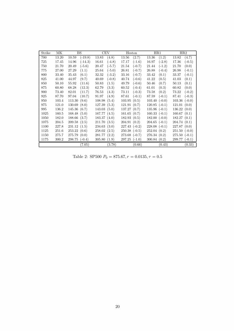
[ Table 2 about here ]
Table 2 shows the optimization results on a cross section of option prices for
Black and Scholes, CEV, Heston, and HR models for both volatility functions (9)
(label HR1) and (10) (label HR2). The second column shows the market prices
of a European put option on SP500 index on the 20th of March 2003, with strikes
specified in the first column and maturity September 2003. As an annual interest rate
we considered the corresponding T-bill r = 0.0135 available from Federal Reserve
Statistical Releases. We choose a quite long time to maturity6 remembering that
smile effect decreases with it (see e.g. (DERMAN and KANI 1994)), thus simplyfing
the task of pricing on such a broad range of moneyness values. On the right of each
estimated price we report the percentage relative error between parentheses, while
5in order to avoid difficulties we used a robust interpolation technique, see the reference for details.6τ = 0.5289256 considering one year of 242 trading days.
12
the last row shows the mean of the absolute percentage relative error across the
strikes for each model.
We see that the Black and Scholes model can be reasonably good on a small
number of strikes around the current stock value, but completely fails to fit a large
cross section of option prices. On the other hand, considering the small number
of parameters used, the CEV model performs far better and it is easy to calibrate.
Sadly, theoretically it is not able to explain the change over time in the direction of the
implied volatility skews observed by (RUBINSTEIN 1985). Both the Heston model
and the HR model provide an excellent fit at the cost of an increased computational
burden. However, for this dataset the simple specification HR2 provides the best fit
using the simple volatility specification (10) and just three parameters.
The model performance was tested against a variety of other datasets, consider-
ing different underlying assets, multiple maturities and the behaviour of parameters
through time. Without entering into the econometric details, in general HR per-
formances are comparable with if not superior to other commonly used stochastic
volatility models.
5 Why no asymptotics?
We have seen how the price f(t, U, Z) at time t of a European derivative solves a
PDE, which we can compute numerically, but this is a time-consuming business, and
the model would be much easier to use if there were some simple asymptotics. The
natural form to look for would be to express the derivative price as the Black-Scholes
price plus some (smaller order) correction, since the Black-Scholes price is what we
could obtain if the volatility were constant. But to obtain an asymptotic, we need
to identify some small parameter and expand in that.
One possibility would be to take λ−1 to be the small parameter, but this has
certain drawbacks. It is true that if λ−1 were small then the offset would typically
be small, and so the volatility would be close to σ(0); but then in times that are O(1)
the diffusion S will quickly settle down to its invariant distribution, and the price will
lose dependence on the initial value of the offset, becoming in effect a Black-Scholes
13

price with an averaged variance. Moreover, as Figure 1 shows, the volatility does
not appear to be close to a constant (at least in the real-world measure).
Another possibility would be to keep λ fixed, but instead to take the volatility of
the form σ(εS) for small ε; this way, the initial value of the offset could continue to
influence prices for some time, but the correction will itself solve a PDE, which is no
easier than the PDE for calculating the price.
But however one tries to develop an asymptotic, Figure 1 ruins the attempt;
offsets are not generally small, and volatility is not approximately constant, so no
asymptotic based on assuming either of these properties can succeed.
The paper of (HUBALEK, TEICHMANN, and TOMPKINS 2004) obtains an
asymptotic for a model where σ(s) = σ0(√
εs) for some small ε; again in view of
Figure 1 it seems unlikely that any such asymptotic will explain the data well, and
few results of fitting this model are reported in their work.
6 Conclusions
This study has tested the model of HR at two levels. Firstly, we have investigated
whether there is any apparent dependence of volatility on offset; fitting quadratic
functions of offset to volatility data shows a conclusive dependence. Secondly, we
have attempted to fit some simple functional forms to the dependence of volatility
on offset, using options data on the SP500. The quality of fit is excellent, generally
twice as good as the popular Heston model, and within the bid-ask spread. The
numerics involved are somewhat more complicated than (for example) pricing in the
Heston model using transform methods; nevertheless, given that one has available
good finite-difference code for sparse linear systems, the development time is not
great, and the run times for solving the PDE are of the order of 0.1s. In addition
to the good fit, the model has two advantages at a theoretical level: it is complete
(so no arbitrary choices of market price of risk are needed); and option prices do not
depend solely on spot, strike and expiry, so that different skew/smile profiles may
be generated for the same spot, depending on the value of the offset. This means in
particular that it may be possible to avoid time-dependent implied-volatility surfaces
14
as a way to explain observed prices. Further work is needed to evaluate this model
in this respect, but we conclude from the present study that its performance is good
enough already to justify it.
References
ANDERSEN, T. G., H. CHUNG, and B. E. SØRENSEN, 1999, Efficient method ofmoments estimation of a stochastic volatility model: a monte carlo study, Journal
of Econometrics 91, 61–87.
BAKSHI, G., C. CAO, and Z. CHEN, 1997, Empirical performance of alternativeoption pricing models, The Journal of Finance 52, 2003–2049.
BATES, D. S., 2003, Empirical option pricing: a retrospection, Journal of Econo-
metrics 116, 387–404.
BLACK, F., 1976, Studies of stock price volatility changes, Proceedings of the 1976Meetings of the American Statistical Association, 177-181.
, and M. SCHOLES, 1973, The pricing of options and corporate liabilities,Journal of Political Economy 81, 637–659.
BLATTBERG, R. C., and N. J. GONEDES, 1974, A comparison of the stable andstudent distributions as statistical models for stock prices, Journal of Business 47,244–280.
BOYLE, P., 1977, Options: A monte carlo approach, Journal of Financial Economics
4, 323–38.
, M. BROADIE, and P. GLASSERMAN, 1997, Monte Carlo methods forsecurity pricing, Journal of Economic Dynamics and Control 21, 1267–1321.
BRENNAN, M. J., and E. S. SCHWARTZ, 1978, Finite difference method and jumpprocesses arising in the pricing of contingent claims, Journal of Financial and
Quantitative Analysis 13, 461–474.
CHERNOV, M., A. R. GALLANT, E. GHYSELS, and G. TAUCHEN, 2003, Alter-native models for stock price dynamics, .
CORRADI, V., 2000, Reconsidering the continuous time limit of the GARCH(1,1)process, Journal of Econometrics 96, 145–153.
COURTADON, G., 1982, A more accurate finite difference approximation for thevaluation of options, Journal of Financial and Quantitative Analysis 17, 697–703.
COX, J. C., and S. A. ROSS, 1976, The valuation of options for alternative stochasticprocesses, Journal of Financial Economics 3, 145–166.
DERMAN, E., and I. KANI, 1994, Riding on the smile, RISK 7, 32–39.
DUAN, J. C., 1995, The GARCH option pricing model, Mathematical Finance 5,13–32.
DUFFIE, D., 2001, Dynamic Asset Pricing Theory (Princeton University Press:Princeton) third edn.
15
DUMAS, B., J. FLEMING, and R. E. WHALEY, 1998, Implied volatility functions:Empirical tests, The Journal of Finance 53, 2059–2106.
FOUQUE, J. P., G. PAPANICOLAU, and K. R. SIRCAR, 2000, Derivatives in
Financial Markets with Stochastic Volatility (Cambridge University Press: Cam-bridge).
GHYSELS, E., A.C. HARVEY, and E. RENAULT, 1996, Stochastic Volatility, vol. 14of Statistical Methods in Finance . pp. 119–191 (Handbook of Statistics, North-Holland).
GLASSERMAN, P., 2003, Monte Carlo Methods in Financial Engineering (Springer-Verlag: New York).
HESTON, S. L., 1993, A closed-form solution for options with stochastic volatilitywith applications to bond and currency options, Review of Financial Studies 6,327–343.
HOBSON, D. G., and L. C. G. ROGERS, 1998, Complete models with stochasticvolatility, Mathematical Finance 8, 27–48.
HUBALEK, F., J. TEICHMANN, and R. TOMPKINS, 2004, Flexible completemodels with stochastic volatility generalizing Hobson-Rogers, submitted.
HULL, J., and A. WHITE, 1987, The pricing of options on assets with stochasticvolatilities, Journal of Finance 42, 281–300.
, 1990, Valuing derivative securities using the explicit finite difference method,Journal of Financial and Quantitative Analysis 25, 87–100.
JACKWERTH, J. C., and M. RUBINSTEIN, 1996, Recovering probability distribu-tions from option prices, The Journal of Finance 51, 1611–1631.
KLOEDEN, P. E., and E. PLATEN, 1999, Numerical Solution of Stochastic Differ-
ential Equations (Springer: Berlin).
PLATEN, E., and M. SCHWEIZER, 1998, On feedback effects from hedging deriva-tives, Mathematical Finance 8, 67–84.
ROGERS, L. C. G., and S. E. SATCHELL, 2000, Does the behaviour of the assettell us anything about the option price formula?, Applied Financial Economics 10,37–39.
RUBINSTEIN, M., 1985, Nonparametric tests of alternative option pricing modelsusing all reported trades and quotes on the 30 most active CBOE option classesfrom august 23, 1976 through august 31, 1978, The Journal of Finance 11, 455–480.
SCHRODER, M., 1989, Computing the constant elasticity of variance option pricingformula, The Journal of Finance 44, 211–219.
SCHWARTZ, E. S., 1977, The valuation of warrants: Implementing a new approach,Journal of Financial Economics 4, 79–93.
SCHWERT, G. W., 1989, Why does volatility change over time?, The Journal of
Finance 44, 1115–1153.
16
SCOTT, L. O., 1987, Option pricing when the variance changes randomly: Theory,estimation, and an application, Journal of Financial and Quantitative Analysis
22, 419–438.
TAVELLA, D., and C. RANDALL, 2000, Pricing Financial Instruments: the Finite
Difference Method (Wiley: New York).
TOMPKINS, R. G., 2001, Stock index futures markets: Stochastic volatility modelsand smiles, Journal of Future Markets 21, 43–78.
WIGGINS, J. B., 1987, Option values under stochastic volatility. theory and empir-ical estimates, Journal of Financial Economics 19, 351–372.
17
−0.21 −0.065 0.080
1
2
3
4
5
6x 10
−4 λ = 10.0
−0.16 −0.04 0.080
2
4
6
8x 10
−4 λ = 20.0
−0.12 −0.025 0.070
0.2
0.4
0.6
0.8
1
x 10−3 λ = 40.0
−0.1 −0.015 0.070
0.2
0.4
0.6
0.8
1
1.2
1.4x 10
−3 λ = 60.0
−0.09 −0.01 0.070
0.5
1
1.5
x 10−3 λ = 80.0
−0.08 −0.01 0.060
0.5
1
1.5
2x 10
−3 λ = 100.0
Figure 1: Offset vs volatility, SP500 index 1993-2002.
18
λ Term Bounds PE λ Term Bounds PE
a 1.4062 1.5078 1.4570 a 1.2636 1.4329 1.348310.0 b -10.4201 -8.4427 -9.4314 60.0 b -5.6929 1.0993 -2.2968
c 33.0946 53.5770 43.3358 c 326.2475 463.6645 394.9560
a 1.3570 1.4824 1.4197 a 1.2360 1.4177 1.326920.0 b -11.4611 -7.9622 -9.7116 80.0 b -4.2323 3.7437 -0.2443
c 83.8240 129.0635 106.4437 c 449.9151 630.4401 540.1776
a 1.2643 1.4128 1.3386 a 1.2167 1.4097 1.313240.0 b -9.5973 -4.3470 -6.9722 100.0 b -2.9359 6.1401 1.6021
c 249.9483 339.9986 294.9734 c 559.4291 782.6407 671.0349
Table 1: SP500 index 1993-2002 regressions. Bounds are the 95% confidence intervals for thepoint estimates PE, all numbers are multiplied by 1.0E4.
19
Strike MK BS CEV Heston HR1 HR2
700 13.20 10.59 (-19.8) 13.83 (4.8) 13.56 (2.7) 13.36 (1.2) 13.82 (4.7)725 17.45 14.96 (-14.3) 16.61 (-4.8) 17.17 (-1.6) 16.97 (-2.8) 17.36 (-0.5)750 21.70 20.49 (-5.6) 20.47 (-5.7) 21.54 (-0.7) 21.44 (-1.2) 21.70 (0.0)775 27.00 27.29 (1.1) 25.64 (-5.0) 26.81 (-0.7) 26.88 (-0.4) 26.98 (-0.1)800 33.40 35.43 (6.1) 32.32 (-3.2) 33.16 (-0.7) 33.42 (0.1) 33.37 (-0.1)825 41.00 44.97 (9.7) 40.69 (-0.8) 40.74 (-0.6) 41.22 (0.5) 41.03 (0.1)850 50.10 55.92 (11.6) 50.83 (1.5) 49.79 (-0.6) 50.46 (0.7) 50.13 (0.1)875 60.80 68.28 (12.3) 62.79 (3.3) 60.52 (-0.4) 61.01 (0.3) 60.82 (0.0)900 73.40 82.01 (11.7) 76.53 (4.3) 73.11 (-0.3) 73.58 (0.2) 73.22 (-0.2)925 87.70 97.04 (10.7) 91.97 (4.9) 87.61 (-0.1) 87.59 (-0.1) 87.41 (-0.3)950 103.4 113.30 (9.6) 108.98 (5.4) 103.95 (0.5) 103.40 (-0.0) 103.36 (-0.0)975 121.0 130.69 (8.0) 127.39 (5.3) 121.91 (0.7) 120.85 (-0.1) 121.01 (0.0)995 136.2 145.36 (6.7) 143.03 (5.0) 137.27 (0.7) 135.96 (-0.1) 136.22 (0.0)1025 160.5 168.48 (5.0) 167.77 (4.5) 161.65 (0.7) 160.33 (-0.1) 160.67 (0.1)1050 182.0 188.66 (3.7) 183.37 (4.0) 182.93 (0.5) 182.00 (-0.0) 182.27 (0.1)1075 204.5 209.58 (2.5) 211.70 (3.5) 204.91 (0.2) 204.65 (-0.1) 204.74 (0.1)1100 227.8 231.12 (1.5) 234.63 (3.0) 227.43 (-0.2) 228.08 (-0.1) 227.87 (0.0)1125 251.6 253.22 (0.6) 258.02 (2.5) 250.38 (-0.5) 252.04 (0.2) 251.50 (-0.0)1150 275.7 275.79 (0.0) 281.77 (2.2) 273.68 (-0.7) 276.34 (0.2) 275.50 (-0.1)1175 300.2 298.75 (-0.4) 305.80 (1.9) 297.25 (-1.0) 300.84 (0.2) 299.77 (-0.1)
(7.05) (3.78) (0.66) (0.43) (0.33)
Table 2: SP500 P0 = 875.67, r = 0.0135, τ = 0.5
20
Recommended