
i
PUBLIC DEBT, TAX REVENUE AND GOVERNMENT EXPENDITURE IN
KENYA: 1960-2012
KIMINYEI FELIX KIMTAI
A RESEARCH PROJECT SUBMITTED TO THE SCHOOL OF ECONOMICS IN
PARTIAL FULFILMENT OF THE REQUIREMENTS FOR THE AWARD OF
MASTER OF ARTS (ECONOMICS) DEGREE OF THE UNIVERSITY OF
NAIROBI.
OCTOBER 2014

ii
DECLARATION
This research project is my original work and has not been presented for a degree award
in any other University or Institution
Signature……………………….. Date……………………………….
Name : Kiminyei Felix Kimtai
Reg No : X50/63752/2011
This research project has been submitted for examination with our approval as University
supervisors
Signature...................................... Date...............................................
Name : Prof. Nelson Wawire
Signature...................................... Date...............................................
Name : Dr. John Gathiaka

iii
DEDICATION
My parents and the entire family of Mr. Charles Kiminyei for their unending dedication
and commitment in fighting the ravages associated with illiteracy.

iv
ACKNOWLEDGEMENTS
Thanks to The Almighty God for the gift of Life and Good Health. The author would like
to recognize sincere appreciation stemming from several players that in any manner made
this research project possible, even with underlying challenges in mentioning all in
person. Specifically, sincere appreciation goes to; supervisors, Prof. Nelson Wawire and
Dr. John Gathiaka, to whom a lot is still owed for their time devoted going through a
number of drafts while at the same time providing significant guidelines that equally
played a huge role in shaping the understanding of main tenets guiding the writing of a
research project ; entire staff at Kenya Bankers Association for being hospitable-
specifically Mr. Jared Osoro, The Director Research and Policy at the Kenya Bankers
Association (KBA) Centre for Research on Financial Markets and Policy (CRFMP) for
extending and offering an internship opportunity upon which continued learning was
inevitable ; colleagues, a good lot whom have been out of contact since completion of
coursework yet their insight in developing interest into this topic would not be neglected
as such ; institutions including the Kenya national bureau of statistics (KNBS) library, the
national treasury library and the University of Nairobi (UON) school of economics
graduate library for their resourceful assistance; and all other persons that directly or
indirectly made this research project successful.

v
TABLE OF CONTENTS
DECLARATION .......................................................................................................................... ii
DEDICATION ............................................................................................................................ iii
ACKNOWLEDGEMENTS ........................................................................................................ iv
TABLE OF CONTENTS ............................................................................................................. v
LIST OF TABLES .................................................................................................................... viii
LIST OF FIGURES ..................................................................................................................... ix
ABBREVIATIONS AND ACRONYMS .................................................................................... x
OPERATIONAL DEFINITION OF TERMS ............................................................................. xi
ABSTRACT .............................................................................................................................. xiii
CHAPTER ONE: INTRODUCTION .......................................................................................... 1
1.1 Background ...................................................................................................... 1
1.1.1 Public Debt, Tax Revenue and Government Expenditure ............................... 4
1.1.2 Trends in Public Debt, Tax Revenue and Government Expenditure ............... 8
1.2 Statement of the Problem ............................................................................... 11
1.3 Research Questions ........................................................................................ 12
1.4 Objectives ...................................................................................................... 13
1.5 Significance of the Study ............................................................................... 13
1.6 Scope and Organization of the Study ............................................................ 14
CHAPTER TWO: LITERATURE REVIEW ............................................................................ 15
2.1 Introduction .................................................................................................... 15
2.2 Theoretical Literature..................................................................................... 15
2.2.1 Classical Theory of Public Debt .................................................................... 15
2.2.2 Keynesian Debt Theory ................................................................................. 18
2.2.3 Lerner’s Theory of Functional Finance ......................................................... 21
2.2.4 Tax Smoothing ............................................................................................... 23
2.2.5 Ricardian Equivalence ................................................................................... 25

vi
2.3 Empirical Literature ........................................................................................ 30
2.4 Overview of the Literature .............................................................................. 41
CHAPTER THREE: METHODOLOGY ................................................................................... 43
3.1 Introduction ..................................................................................................... 43
3.2 Theoretical Framework ................................................................................... 43
3.3 Model Specification ........................................................................................ 46
3.4 Definition and Measurement of Variables ...................................................... 49
3.5 Data Type, Source and Refinement ................................................................ 49
3.6 Stationarity Analysis ....................................................................................... 50
3.7 Cointegration Analysis ................................................................................... 51
3.8 Distribution and other Diagnostic Tests ......................................................... 54
3.9 Data Analysis .................................................................................................. 55
3.9.1 Correlation Analysis ....................................................................................... 55
3.9.2 Vector Error Correction Model ....................................................................... 57
3.9.3 Granger Causality ........................................................................................... 58
3.9.4 Impulse Response Functions .......................................................................... 59
3.9.5 Forecasting ...................................................................................................... 60
CHAPTER FOUR: EMPIRICAL FINDINGS ........................................................................... 61
4.1 Introduction ..................................................................................................... 61
4.2 Descriptive Statistics ....................................................................................... 61
4.3 Findings for Stationarity Analysis .................................................................. 63
4.4 Findings for Cointegration Analysis ............................................................... 64
4.5 Distribution and other Diagnostic Test Results .............................................. 65
4.6 Regression results ........................................................................................... 66
4.6.1 The relationship between public debt and government expenditure .............. 74
4.6.2 The relationship between public debt and tax revenue ................................... 75

vii
CHAPTER FIVE: SUMMARY, CONCLUSIONS AND POLICY IMPLICATIONS ............. 77
5.1 Introduction ..................................................................................................... 77
5.2 Summary ......................................................................................................... 77
5.3 Conclusions ..................................................................................................... 78
5.4 Contribution to Knowledge ............................................................................ 80
5.5 Policy Implications ......................................................................................... 80
5.6 Limitations and Areas for Further Research ................................................... 81
REFERENCES ........................................................................................................................... 83
APPENDICES ............................................................................................................................ 94

viii
LIST OF TABLES
Table 4.1: Results for Vector Error Correction Model (VECM) ......................................... 67
Table 4.2: Results for VECM Short run model ................................................................... 68
Table 4.3: Results for Forecast Error Variance Decomposition (FEVD) ............................ 72
Table A1: Descriptive Statistics: Public debt, tax revenue and government expenditure ... 94
Table A2: ADF and PP Unit Root Test Results: Public debt, tax revenue and government
expenditure ........................................................................................................................... 94
Table A3: Johansen Cointegration Test Results .................................................................. 95
Table A4: Eigenvalue stability condition ............................................................................. 95
Table A5: Results for Granger causality tests: Public debt, tax revenue and government
expenditure ........................................................................................................................... 96
Table A6: Results for correlation analysis: Public debt, tax revenue and government
expenditure ........................................................................................................................... 96
Table A7: Data for Public debt, tax revenue and government expenditure, 1960-2011....103

ix
LIST OF FIGURES
Figure 1.1: Budget deficit, Public debt, Tax revenue and Government expenditure (Percent
of GDP) ................................................................................................................................ 10
Figure A1: Trends in Public debt, tax revenue and government expenditure, 1960-2011 ... 97
Figure A2: Residual plots for cointegration equations ......................................................... 97
Figure A3: Graph for response of public debt to innovations in tax revenue ...................... 98
Figure A4: Graph for response of tax revenue to innovations in public debt ...................... 98
Figure A5: Graph for response of public debt to innovations in government expenditure .. 99
Figure A6: Graph for response of government expenditure to innovations in public debt .. 99
Figure A7: Graph for response of public debt to innovations in public debt ..................... 100
Figure A8: Ex ante forecasts, public debt tax revenue and government expenditure
components, 2001-2011 ..................................................................................................... 101
Figure A9: Out-of sample dynamic forecasts, 2011-2030 ................................................. 102

x
ABBREVIATIONS AND ACRONYMS
AD Aggregate Demand
AIC Akaike Information Criterion
CBK Central Bank of Kenya
CPI Consumer Price Index
DSR Debt Service Ratio
GDP Gross Domestic Product
GE Government Expenditure
GR Tax Revenue
HIPC Highly Indebted Poor Countries
KES Kenyan Shilling
KNBS Kenya National Bureau of Statistics
MEI Marginal Efficiency of Investment
MPC Marginal Propensity to Consume
PD Public Debt
PVBC Present Value Borrowing Constraint
REPO Repurchase Order
SSA Sub-Saharan Africa
VAR Vector Autoregression
VECM Vector Error Correction Model

xi
OPERATIONAL DEFINITION OF TERMS
Budget deficit is higher government expenditure over tax revenue.
Confidence interval is a measure of reliability of the estimate that a population
parameter falls between two set values.
Consumer price index is a measure of the effect of inflation on purchasing power of a
basket of goods consumed by the consumer.
Correlation is a measure of statistical degree and type of relationship between any two
or more time series over a period of time.
Economy is the entire network of producers, distributors and consumers of goods and
services in a national community.
Government expenditure is money that a government spends.
Government is a group that exercises sovereign authority over a nation.
Government revenue is income a government receives.
Model is an abstraction from reality based on theory and having a set of logical and
quantitative relationships.
Policy is a plan of action.
Public debt is total borrowing by the government to finance its expenditure.
Seignorage is government revenue due to printing money.
Splicing is joining short series of data to obtain longer series.

xii
Tax is compulsory transfer of money from private individuals, institutions or groups to
the central government for public purposes.
Tax revenue is government income due to taxation.

xiii
ABSTRACT
In lieu of rising budget deficits in many countries across the world, driven by tax revenue
insufficiency in financing government expenditure, many governments have continued to
accumulate public debt due to the financing of budget deficits. In the long run, however,
persistent budget deficits as well as debt accumulation are unsustainable and pose several
problems to the economy including inflationary spirals, depressed growth, higher
associated poverty levels and consequently fiscal crisis. To offer any policy prognosis
towards controlling and consequently reducing budget deficit as well as public debt and
associated problems requires an understanding of the relationship between public debt,
tax revenue and government expenditure. This study utilized the present value borrowing
constraint (PVBC) to study the relationship between public debt, tax revenue and
government expenditure in Kenya, for 1960-2011. Annual time series data for total public
debt, tax revenue and government expenditure were converted into their respective real
values by dividing their respective nominal values by the Consumer Price Index (CPI).
Data was collected from Kenya economic surveys from 1960-2013. Because data was
available in fiscal years, it was converted to calendar years by splicing. Augmented
Dickey Fuller and Philips Perron unit root tests were employed to establish the stationary
properties of the series while the Johansen and Juselius co-integration techniques were
used to determine presence of linear long run economic relationships in the series.
Because cointegrating relationships invalidated ordinary estimation techniques, to
achieve these relationships, which formed the objectives of the study, data was analysed
using vector error correction model (VECM) with correlation analysis. The study found
that public debt responds to both tax revenue and government expenditure particularly in
the long run. There was strong positive correlation between public debt tax revenue and
government expenditure and all correlation coefficients were statistically significant.

1
CHAPTER ONE
INTRODUCTION
1.1 Background
Budget deficits have been rising recently and have been associated with rising
government expenditures relative to revenue capacity. For example, expenditures on
salaries, wages, and even interest on debt have been growing rapidly and can be traced
back to the first and second World Wars when the share of spending in GDP rose to over
45 and 60 percent in that order in Britain and across Nations (Hjerpe et al., 2007).
Running budget deficits, however, has received defense from a political economy
perspective – that budget deficits are used to control repercussions that may result from
sharp changes in the rates of taxes. In this sense, Battaglini and Coate (2008) argue that
governments act much the same as individuals hence their expenditure needs change
from time to time. Thus, in time of high expenditure demands governments would run
budget deficits. The converse would be true in times of low government expenditure
needs, paving way for budget surpluses (excess of tax revenues over government
spending).
Along this line of argument, there has been increasing proponents for balanced budgets
calling for modest deficits during times the economy is doing badly and surpluses when
the economy is in a boom. The underlying argument is that fiscal policy ought to be
brought to the channel that is largely seen to be sustainable in both the short and long run.

2
In its real sense, sustainability would mean deficits remain low and even though they
grow with time, the rate of growth is below the rate of GDP growth. In this perspective,
the economy can sustain the budget deficits.
Towards financing these government budget deficits, fiscal authorities have always
resorted to and relied on borrowing from the private sector (domestic and foreign) using
various instruments at their disposal. Other forms of budget deficit finance, in any case,
exist, for example seignorage where government turns on the printing press. But it seems
fiscal authorities have either exercised caution in dealing with this mode of deficit
finance or have attempted totally to keep away from it. This particularly has to do with
the complexities1 associated with the printing of money.
In the context of these complexities, the desirability and reliability of borrowing in
budget deficit finance is evident. This though does not mean public debt is extremely
safe. Persistent accumulation of public debt beyond levels deemed sustainable is known
to cause difficulty in adjustment of fiscal variables especially through their effects on
Gross Domestic Product (GDP) via private investment (Cottarelli and Schaechter, 2010).
Second, public debt can involve transfer of resources from the private sector into
1 Berneim (1989) and also Mankiw (1989) on the theory of optimal seignorage discussed
in detail how the arising inflation, an outcome of printing money would interact with a
tax system consequently creating significant distortions, randomness and uncertainty in
the economic environment. Moreover, inflation (a tax on money) and high payment
frequencies coupled also with administration costs of this tax would increase transaction
costs and exacerbate social (welfare) losses.

3
unproductive uses that would affect the rate of capital formation (Araujo and Martins,
1999; Carneiro, Faria, and Barry, 2005).
Along with rising budget deficits, revenues have grown slowly2 (or have been falling), a
pattern in stark contrast to that in expenditure. This is despite the fact that governments
rely on such revenues that are raised mainly through taxation to finance government
expenditure programs on defence, infrastructure and social safety net programs of
education and health for example, which are seen to have more productivity and
efficiency gains in directly linking objectives to outcomes. The argument behind this
reliance on taxation has to do with ease of manipulating tax rates to fit desired objectives.
The reality, however, is that this imposes tax burdens to society which lead to welfare
losses. Nevertheless, reliance on taxation is insufficient in financing government
expenditure and is the reason behind budget imbalances (deficit or surplus). Specifically,
most governments run budget deficits due to higher government expenditure relative to
tax revenues.
Given the roles played by both public debt and tax revenue in financing the fiscal/budget
deficit and government expenditures, the relationship between public debt, tax revenue
and government expenditure is the main concern of this study for the purpose of drawing
policy implications on fiscal deficit and public debt control and/or reduction.
2 Slow growth in revenues has been attributed to reliance on few sources of the same like
income tax and trade taxes (see Wawire, 2011). In addition, it is also attributed to lack of
fiscal discipline and information on the functions of tax revenue.

4
Understanding this relationship is important in the following ways: First, this relationship
links the size of government, level of public deficits and the structure/pattern of taxation
and expenditure (Hussain, 2004). In addition, this relationship is passed on to fiscal
policy which is significant in the government tax and expenditure structure/patterns and
plans and therefore aids in effective fiscal policy design. Second, in analysing the role
played by government in the distribution of resources, this relationship ceteris paribus, is
critical in aiding design and implementation of sound fiscal policy for rapid, sustained
social ― economic growth and development (Chang, 2009; Obioma and Ozighalu,
2010). Indeed, this relationship is critical in understanding the causes, outcomes and
future paths/directions of government budget deficit and hence drawing the optimal
strategy/policy framework for both deficit control and deficit reduction (Sadiq, 2011; Al-
Zeaud, 2012). In particular, this study examined these relationships over the period 1960-
2011.
1.1.1 Public Debt, Tax Revenue and Government Expenditure
Most governments have sustained their reliance on borrowing in financing excess of
government expenditure over revenues. Governments perhaps do so to ensure
implementation of government expenditure programs that are vital to the overall
productivity of the economy. It is worth noting that fiscal deficits arising when
government expenditures are in excess of revenues raise a number of issues. They can be
used by relevant authorities to affect the direction of the economy. If the rise in the
fiscal/budget deficit is due to rising development expenditure for example on critical
5
infrastructure initiatives like roads, railway, among others, this has the potential of
reducing poverty through increasing productivity and reducing unemployment
particularly in the long run.
However, a number of analysts particularly economists trace almost every economic
illness to budget deficits. Specifically, persistent increases in the budget deficit has the
potential of causing high inflation, low investment, low consumption and consequently
low economic growth, in the long run. Overall, the effect is raising levels of poverty,
therefore with low living standards and consequently leading to loss in societal welfare.
In effect, this is not the end of the cycle. Fiscal deficit finance involves debt contracting.
Public debt is distributed both as internal and external debt. While internal debt
instruments including Treasury bills and bonds are commonly used by governments in
financing various operations including development aspects of the economy like
supporting huge infrastructure development initiatives which increase capital stock
formation, they nonetheless serve as safe and attractive investments available to the
public promising some fixed and attractive rates of return.
Internal debt instruments can also be used to affect the economy in terms of increasing or
reducing economic activity depending on the state of health of the economy. However,
use of internal debt instruments lead to competition for fixed private savings held by
individuals pushing up market rates of interest and therefore in the long run will crowd
out private investments and lead to low capital formation. Low capital formation today

6
means depressed economic growth in future. Use of external debt is neither safer, it
carries with it the harm to the current account in the balance of payments. The current
account worsens (current account deficit increases) which in turn leads to appreciation in
the exchange rate. Exports become expensive with appreciation while imports become
cheap leading to falling net exports (Mehmood and Sadiq, 2010).
In general, public debt accumulation raises two major issues as regards fiscal deficit
finance – debt overhang and loan repayments. Debt overhang is the disincentives to
investments due to the threat from high debt so that a lot of resources are channelled to
repaying debt. Investors will become sceptical to undertake any investments in a country
which might harm future growth prospects. That is, when investment is
discouraged/reduced/negatively affected, the main possible outcome is reduced growth
both in the present time and in future since a lower capital stock today and in future
would reduce the size of the economy from what it would be , all else equal. On the other
hand, debt (the principal amount) must be repaid at some time/point as well as interest on
debt. In particular, interest payments will either need increase in tax rates hence raising
tax burdens, or increase inflation whenever debt monetization is resorted to.
Thus, increased efforts into repayment of debt lead to misallocation of resources,
increases in poverty, as well as reduction in economic growth since a lot of emphasis is
placed on debt and interest repayment rather than improving the general state of the
economy.

7
Budget deficits also create various trade-offs between various variables. For example, for
the case of growing budget deficits as well as growing public debt, the most likely
solution would be to cut government expenditure, raise taxes or both ways in order to
achieve sustainability. In the present period, a huge reduction in government expenditure
or rise in taxes would be highly desirable to be able to spread these changes with time.
All in all, public debt is not the only means to finance the deficit, other ways exist, for
example seignorage. But either way used, reducing budget deficits is contractionary in
the short run resulting to increasing unemployment and reducing output (Labonte, 2012).
So government or relevant authorities need to examine these trade-offs carefully in
devising policies aimed at reducing the deficits.
Public debt, tax revenue and government expenditure are therefore closely interrelated
and not easily separable. Both public debt and tax revenue are used to finance
government expenditure projects say on infrastructure, social sectors, among others
broadly classified based on their recurrent or/and development aspects that are vital
ingredients in stimulating demand therefore increasing output and reducing
unemployment. While both public debt and taxes represent shift of resources from the
private into the public sector, one distinctive feature between these components of
government finances is that taxes are usually seen as necessary transfers yet public debt
are transfers that are voluntary in nature.

8
Thus, when public debt and taxes are to be chosen by the public, the public usually
chooses public debt financing. The reason is that raising taxes to finance government
expenditure is usually socially undesirable hence the reason to resort to public debt. Also,
public goods have characteristics of non-exclusion (practically impossible to exclude a
person from enjoying them, say public road or public health facility) so that people even
opt for reduction in taxes as the free rider problem comes to play. The choice of debt
financing has to do with low political cost associated with it. And it is this reason that
even politicians run huge budget deficits prior to obtaining elected offices knowing the
public has fiscal illusion ― overestimating the benefits accruing in the present period and
underestimating the costs associated with future tax burdens.
1.1.2 Trends in Public Debt, Tax Revenue and Government Expenditure
In nominal terms, public and publicly guaranteed debt and its components (domestic and
external debt) sustained an upward trend between 2011 and 2012 to stand at Kshs. 1.6
trillion. The composition was 52.6 % domestic debt while 47.4 % was external debt. It is
good noting that debt was financing a budget deficit of Kshs. 117.8 billion and Kshs.
181.5 billion in 2011 and 2012, respectively. As a percent of GDP, even though public
debt declined by 20.4 % with its respective components following cue, the decline in
external debt, however, is so pronounced at 10.7 % compared to that of domestic debt at
5.8% and shows government debt restructuring policy towards more long term domestic
debt components. Government debt management strategy is also meant to cushion the

9
risks associated with use of external debt instruments and short term debt instruments.
This policy is bearing fruit with Treasury bonds consisting 80.9 % of total domestic
government debt securities (Kshs. 687 billion in 2012, an increase of Kshs. 91.2 billion
from 2011), while treasury bills inclusive of Repurchase orders (Repos) consisted 19.1 %
of total government securities in 2012. In addition the 10 year as well as 30 year Treasury
bond rose by 0.8 % in this period. At the same time, interest repayment on domestic debt
rose by Kshs. 14 billion while interest accumulated on external debt rose by Kshs. 0.7
billion with external debt principal repayment amounting to 34.7 billion and debt service
ratio (DSR) rose from 5.1% to 5.25%.
Government revenue inclusive of grants increased to 734.4 billion in 2012 from 679
billion in 2011. As a percent of GDP, this was an increase of 1.7% and on account of
growth in both tax and non-tax revenue sources by Kshs. 74.5 billion (12.7%) and Kshs.
7 billion, respectively. And even with their positive growth, both tax and non-tax revenue
remained below their projected levels on account of depressed economic activity and
special revenue policies meant to reduce the cost of living for example, reduced excise
duty on selected fuels. However, the share of government revenues in total GDP declined
from 24.6 % to 22.3 % in the same period.

10
Source: Republic of Kenya and Central Bank of Kenya (CBK).
Figure 1.1: Budget deficit, Public debt, Tax revenue and Government expenditure
(Percent of GDP)
Finally, expenditure as well as net lending rose to Kshs. 915.9 billion in 2012 from Kshs.
817.1 billion in 2011. While recurrent expenditure rose by Kshs. 57.6 billion to settle at
Kshs. 639.1 billion, development expenditure rose by Kshs. 41.2 billion to settle at Kshs.
276.8 billion, yet both components remained below their projections of Kshs. 697.5
billion and Kshs. 385.4 billion, respectively. And in recent times there has been increased
investments into infrastructure development in line with vision 2030 on creating a
suitable environment for business and investment that saw the a share of development
expenditure in total expenditure rise by approximately 4.9 % from 28.8 % to 30.2 % with
that of recurrent expenditure declining by 1.9 %. The graph shows the current trends in
these variables.

11
1.2 Statement of the Problem
Government fiscal operations saw the budget deficit rise from 4.6 as a percent of GDP in
March 2012 to 5.3 as a percent of GDP in the same month of 2013. Huge and persisting
budget deficits show genuine underlying economic issues, for example loopholes in the
tax system that include tax evasion due to ineffective tax administration. It further
indicates that budget deficit finance, more often than not through resort to public debt –
may not be channelled into those areas that hold more potential in boosting productivity.
Consequently, rising budget deficits to levels that are unsustainable creates the risk of
fiscal crisis where the government is unable to raise revenues to finance its expenditures,
leading to high growth in debt than in Gross Domestic Product (GDP).
Therefore, to be able to offer any policy prescriptions towards controlling and
consequently reducing budget deficit as well as resulting public debt and associated
problems, it is necessary to understand the relationship between public debt, tax revenues
and government expenditure.
The optimal strategy for debt reduction depends on the optimal policy embraced for
budget deficit reduction which in principle entails either expenditure reduction or an
increase in tax revenue. How then might public debt respond to the choice of an
expenditure cut in reducing the budget deficit, all else equivalent? This is the question
this study posed. It sounds reasonable to predict that public debt would reduce. However,
in the last half of 2012 and part of 2013, expenditure cuts proved ineffective in developed
12
nations particularly in the Eurozone (Grauwe and Yuemei, 2013; Aheara, 2012; Grauwe
and Yuemei, 2012; Kiguel, 2012) as it led to slow economic growth, low tax revenues,
deflation and consequently rising public debt in countries such as Greece, Spain, and
Ireland. Upon this background, it is evident that the effects of expenditure cuts (or tax
increases) may not be straight forward, and the study sought to empirically contribute to
the debate.
Among previous studies that attempted to address the relationship between public debt,
tax revenue and government expenditure in Kenya is Ghartey (2012), who studied
exclusively the relationship between tax revenue and government expenditure and
Kanano (2006) who studied the determinants of growth in government expenditure and
not the relationship between public debt, tax revenue and government expenditure per se.
This relationship hence remains an essential matter of empirical study, a gap this study
sought to fill.
1.3 Research Questions
The research questions this study sought to answer are:
(i) What is the relationship between public debt and government expenditure?
(ii) What is the relationship between public debt and tax revenue?
(iii) What policy implications can be drawn from the study?

13
1.4 Objectives
The objectives of this study are:
(i) To examine the relationship between public debt and government expenditure
(ii) To examine the relationship between public debt and tax revenue
(iii) Based on the findings, draw policy implications
1.5 Significance of the Study
First, this study brings additional knowledge to the field of government finance in Kenya
specifically concerning the relationship between public debt, tax revenue and government
expenditure. Given that previous studies are few, for example Ghartey (2012) and
Kanano (2006) and with the recent studies devoting rather to explore economic growth
and government expenditure, for instance Kipkosgei (2011) and Kibe (2009), it is
evident that this study bears great significance in contributing to the literature on Kenya
that has a bearing on future research. This is useful to researchers and scholars interested
in pursuing further research on the relationship between public debt, tax revenue and
government expenditure and/or related issues, as a source of reference. Secondly, to
policymakers especially those in government and other public policy institutions if the
finding of this study is anything to go by it will shape the reactions in terms of
implementing both relevant and appropriate policies in the short and long run geared
towards addressing budget deficit and associated debt problems.

14
Third, this study examined the relationship between public debt, tax revenue and
government expenditure over 1960-2011. To the best of the author’s knowledge, there
was no single study in this perspective done in Kenya. A related study was that of
Kanano (2006) and Ghartey (2012). However, Kanano studied the determinants of
government expenditure growth over 1980-2004 while Ghartey examined the relationship
between tax revenue and government expenditure for Kenya, Ethiopia and Nigeria, and
not the relationship between public debt, tax revenue and government expenditure per se.
1.6 Scope and Organization of the Study
This study period is 1960 – 2012. This period is important because a number of events
occurred that had a direct or indirect effect on public debt, tax revenue or government
expenditure. The government implemented expansionary fiscal policies particularly
between 1974 and 1985. These policies, however, had their own problems as budget
deficits rose rapidly even a decade later. Public debt problems could thus be traced into
this period. Other notable events include the oil crisis in 1972/1973, free primary
education in 2003, the post election violence of 2007/2008 and the global financial crisis
of 2008. Furthermore, the Kenyan vision 2030 was designed during this period.
The rest of this study is organized as follows: Chapter two reviews theoretical and
empirical literature with an overview of the literature, chapter three presents the
methodology, chapter four presents the empirical findings while chapter five presents the
summary conclusions and policy implications.
15
CHAPTER TWO
LITERATURE REVIEW
2.1 Introduction
This chapter presents the theoretical and empirical review of literature on the relationship
between public debt, tax revenue and government expenditure.
2.2 Theoretical Literature
2.2.1 Classical Theory of Public Debt
Classical3 (1742-1859) debt theory maintained that debt imposed a burden on future
generations and very high levels of public debt would create national bankruptcy. It was
Buchanan (1958) who made this view clear stating that bondholders acted voluntarily
(not sacrificing) choosing from a number of investment opportunities and in future would
be better off the moment they are paid the principal together with interest. Hence they did
not bear the real burden of debt (burden of debt was a utility loss and not a financial loss).
In addition, public debt was accompanied by a cost; interest payment on debt that
affected net income negatively therefore reduced future standard of living of a borrower
3 The term Classical or Smithian economists does not refer to a particular economist but
rather a school of thought made up of mainstream economists who wrote between 1742
through the early 1930s, and were much more active over 1800-1850. The school of
thought diminished with the onset of the neoclassical economists in about 1900. They
held some common views (beliefs) that have been entangled into a school of economic
thought, upon which the classical debt theory is derived.

16
if it was used to finance high present consumption. Buchanan concluded that public debt
was immoral since it made future generations pay the principal together with interest
towards government expenditure (government spending was seen as unproductive)4
decisions they did not participate themselves (Templeman, 2007).
Classical economists favoured balanced budgets ― all government expenditure financed
by taxation. Running budget deficits and resort to borrowing would be justified only
during national emergencies, say war or a natural disaster. Smith (1776, 1937), in
particular stated that the choice between a tax and public borrowing mattered for capital
accumulation. Since to these economists savings was equal to investment, taxation would
only reduce household expenditures, new investment and consequently new capital
accumulation but would leave the economy’s productive capacity and hence existing
capital stock unaltered. In contrast, however, public borrowing would alter productive
capacity by diverting savings from private investment which was productive, into
unproductive and wasteful uses (Tsoulfidis, 2007). This, simply put was that tax versus
debt finance (and their effects on the economy) were and contrary to Barro’s (1974)
equivalence hypothesis, not equivalent.
4 Classical economists held that public expenditure was unproductive, that is to say,
public expenditure was channelled to useful social functions like paying salaries and
wages and provision of security among others, which although could not be left in the
hands of the private sector, would consume part of the social wealth already produced in
order to provide such functions. This act of taking away from social wealth to provide
for social functions is what rendered public expenditure unproductive.

17
Ricardo (1951), whom a lot is credited on developing the Ricardian equivalence, rejected
as to whether tax and debt finance were equivalent. Ricardo stated explicitly that these
two methods were non-equivalent. In the case of public debt for example, the public did
not view it as equal to a tax cut and would tend to save less compared to when a tax was
really imposed-therefore reducing the rate of capital formation. In the event that capital
accumulation continued to fall, it would do so together with output/income causing
revenues to government generally from taxation and also income tax to respond just the
same way. In response to falling revenues, government would hike the tax rates
attempting to maintain her level of revenues. The outcome was however ugly,
accentuating the fall in capital accumulation and consequently breeding national
bankruptcy.
To Ricardo therefore, there were only two extreme circumstances under which tax and
debt finance were equivalent. First, taxation and borrowing were seen to be only
economically equal, that is saying, the same amount of debt would be paid for by taxes,
for example in a situation when a budget deficit was financing public investment on
infrastructure. Second, taxation and borrowing might be equal only in the short run where
they give forth similar outcome. In the long run, however, while taxation would affect
current income for which it was not clearly established whether such incomes would be
consumed or invested, public borrowing would have devastating effects on the society’s
capacity to accumulate capital by reducing savings that could have been directed into
productive investments.

18
It was Mill (1976) who incorporated the idea of crowding out in the classical debt theory.
To Mill, if debt was being financed by the surplus that was not needed by the private
sector, there was no crowding out. However, crowding out occurred only when the
government and the private sector competed for the same funds eventually causing the
rates of interest (price of capital) to rise. Rising interest was partly due to increasing rate
of profit which happened since borrowing led to falling private capital. Such a fall in
private capital would increase competition among workers and decrease their real wages,
which was equivalent to an increase in the rate of profits. High rates of interest therefore
would cause Investment to fall, and similar trends would be seen in employment and
output, chronically. In addition, Mill did not view public debt as having adverse
consequences to a nation under three cases: If it was foreign debt, when it created savings
that would not have occurred and when borrowing absorbed savings that would have
otherwise been invested in unproductive uses or in foreign nations.
2.2.2 Keynesian Debt Theory
Keynes (1936) position was that the economy had various forces and mechanisms within
it which were pushing it into disequilibria. Hence contrary to the classical economist’s
say’s law, market forces of supply and demand left alone were unable to deliver an
equilibrium with economic and efficiency gains. In particular, the economy was
cyclically unstable and therefore under the threat of fluctuations because investment was
insufficient and saving was very high. This was accounted for by high uncertainty which
rendered market forces insufficient in creating equilibrium with full employment. The

19
only solution to insufficient investment was to incorporate public investment in its place
which would occur through borrowing to finance the budget deficit (Yergin and
Stanislaw, 1998). As the effects of deficit spending for instance public works projects
filtered through the economy, it increased employment together with the purchasing
power. This was what Keynes called the multiplier effect denoted as a reciprocal of (1-c),
where c is the marginal propensity to consume (MPC). The concept of the multiplier was
that people purchased goods and services from the money they were paid being employed
in public works projects hence maintaining or increasing employment.
On the budget position, the central idea of the Keynesian debt theory was simple - there
was no need to force the budget to balance. This was like the government was taking with
one hand from what it was giving with the other. In fact, doing so when the economy’s
health was poor was disastrous. For example, contending to balance the budget in a
recession would aggravate the recession, increase the pace at which output declined,
increase unemployment and consequently create deflation. A recession would need a cut
in taxes and an increase in expenditure to stimulate total (or aggregate) demand. Along
the same line, during a recovery, government should cut spending and increase taxes to
cut total demand and avoid inflation.
Keynesians held that deficits were not supposed to crowd out private investment. To
support this idea, they stated that aggregate demand (AD) increased the returns of private
investment which at any given rate of interest would lead to an increase in total
investment. Therefore, despite the presence of high interest rates, borrowing would foster

20
savings and investment and in the event that consumption increased, it was a result of
unemployed resources which was at the heart the theory (Berheim, 1969). However, there
was only one condition under which borrowing would crowd out investments ― when
the economy was in full employment. This would create displacement of resources,
moving resources from the private into the public sector. Considering availability and
private sector demand for these funds, rising public sector (government) demand for the
same would push the market rates of interest up eventually crowding out private
investment and setting up a recession. Nevertheless, the total effect of interest rates on
total investment, all else equal, would be highly dependent on the demand elasticity of
investment with respect to rates of interest because investment depends on a number of
variables for example the marginal efficiency of investment (MEI) (Malick, 2005).
On debt burden, Keynesians stated that debt did not impose any burden on future
generations. As long as the GDP trajectory and speed looked up, the ratio of public debt
to Gross Domestic Product (GDP) would diminish at a faster rate. That is, high aggregate
demand due to high government expenditure was necessary to diminish debt. In fact, debt
had its advantages and hence was not a burden. To illustrate this point, Keynesians stated
that when government borrowed to finance government expenditure, it was basically
utilizing surplus savings held by the public which would be channelled to productive use
leading to an increase in national output.

21
2.2.3 Lerner’s Theory of Functional Finance
Lerner (1943), stated that government should borrow only if it was in the social interest
for the government to hold more money and the public to hold more government bonds,
which was the entire effect of government borrowing ― efficient when the public might
attempt to lend out their cash leading to low interest rates therefore inducing very high
investments that consequently breeds inflation. Lerner’s (1943) theory is based on what is
called functional finance. Functional finance is judging fiscal policies from their effects
on the economy, irrespective of whether they are sound or unsound. Therefore,
government borrowing as well as debt repayment was primarily used to adjust public
holdings of money and government bonds. Whenever there was a budget surplus,
government could use it to repay part of public debt (if it was desirable to increase money
held by the public and reduce unemployment and government bonds). Similarly, a budget
deficit would be financed by either borrowing or printing money depending on their
desirability in maintaining full employment and preventing inflation. On seignorage,
Lerner stated that it was effected only when it was desirable to implement functional
finance to spend, lend or repay debt. In the author’s definition, printing of money
included borrowing from banks and did not affect total money spent. In addition, printing
money was conditional on new credit money provision by banks based on their additional
government bond holdings.

22
According to functional finance (Lerner, 1943) therefore, high debt was not supposed to
be a threat to society because with the application of the underlying principles of the
theory, the level of total demand was maintained which was necessary for total output to
ensure full employment and also avoid inflation. This means there was no debt burden
either on future or current generations, to which Lerner gave four reasons. First, money
and debt could be allowed to grow together in a certain balance while maintaining the
two laws of functional finance ― checking inflation and maintaining full employment, so
that debt did not grow that fast. Secondly, private investment could be made more
attractive with the main objective of maintaining full employment. This would then
prevent the suspicion of a depression that would make deficit finance decline and hence
debt. Third, high debt meant high private wealth (bonds in the hands of the public); hence
even with taxes unchanged, government had high revenue from income taxes and
bequests. Since this did not result from reduction in spending by the public, it could
therefore be used to repay interest on debt. Fourth, government could tax the rich to avoid
growth in private wealth (government bonds); because the rich did not reduce
consumption much, the effect was low debt ― and similar economic effects to those of
borrowing. In fact, very high debt was unlikely a result of application of functional
finance since according to functional finance (Lerner, 1943), it was natural for debt to
stop growing long before it was close to too high a level like 10,000 billion dollars,
Lerner’s stupendous level. In addition, even though there was no principle for balancing

23
the budget, in the long run the budget would tend to balance as functional finance took
shape so that debt could not balloon to very high levels.
On interest repayment on debt, functional finance (Lerner, 1943) stated that interest could
not be financed solely by taxation unless debt had to be kept at reasonable levels - which
automatically eliminated other forms of interest finance (seignorage and debt). But there
was no sufficient excuse to do this since functional finance kept inflation ― which was
the fear of printing money, on check. Taxation, however, would only be employed when
it was desirable to cut spending and prevent inflation. Otherwise, interest could be repaid
using additional borrowing as long as the public could (and was willing to) lend. If the
public did not wish to lend, they must and would either hoard money or spend. In the
case of hoarding, the government was freed from commitments on future interest
payments on bonds because the public held currency. This would necessitate printing of
money to repay interest and also finance other expenditure needs. When the public spent,
there was no need to borrow and taxation would be effected only when high government
expenditure became a threat in breeding inflation. Tax revenues were then used to repay
the principal debt together with interest.
2.2.4 Tax Smoothing
The theory of tax smoothing is credited to Barro (1979) who encompassed it to fiscal
policy. This theory is based on the assumption that a representative agent - a household,
who works, consumes and saves in a closed economy with no capital has the same finite

24
lifetime together with the government. Tax smoothing implies that fiscal deficits and
public debt tends to be related to cyclical paths of the business cycles and the state which
the economy is at. Specifically, public debt as a ratio of GDP would increase in the
presence of an emergency for example, a war or natural disaster say hurricane, famine
and et cetera; decrease in horizons characterized with lasting peace; fluctuate during
business cycles, that is, increase in a recession and decrease in a recovery towards a
boom. In this theory, government (a benevolent social planner maximizes the utility of
the representative agent) while spending in every period, faced a constraint to keep tax
rates constant to avoid distorting the economy since taxes levied on labor income were
distortionary as they affected the supply of labor (Alessina and Perroti, 1994). This
constraint determined by the intertemporal budget equating the present value of taxes to
the present value of expenditure had a number of implications. It implied that,
government would run budget deficits hence resort to borrowing when spending was high
while a budget surplus would arise when spending was low.
With this background, assuming the usual property of concavity of the consumer’s utility
function, it becomes prudent to predict that if government expenditure is high in the
present period and low in future then from a balanced budget perspective, tax revenues
would have to increase in the present period and decrease in future. But this was not
obviously the case here. According to tax smoothing (Barro, 1979), tax rates must remain
unchanged hence government would run a budget deficit today and a budget surplus in
future that in their respective present values would counterbalance the budget deficit in

25
the present period. Moreover, from the concept of diminishing marginal utility, such a
policy would imply higher welfare gains emanating from lower tax rates in future and
making up for higher tax distortions today. Therefore, tax smoothing was used ideally in
minimizing distortions associated with taxes by running budget imbalances where the
trajectory of spending is exogenous.
2.2.5 Ricardian Equivalence
Barro (1989) presented a theory popularly known as Ricardian equivalence/invariance or
also called tax discounting. This theory was first put forward by David Ricardo. The
theory basically held that tax and public debt financing of government expenditure were
equivalent and hence had the same result. If public debt was financing government
expenditure through a reduction in taxes, future taxes would be high with the same
present value just equal to the tax cut. This was because the government’s budget
constraint equated revenue from taxation and other sources including public debt to
government expenditure (plus interest payments). Hence, there’s no free lunch, total
present value of revenues was fixed by the total present value of expenditures such that it
was a must that government expenditure be paid for, today or in future. If the trajectory in
spending together with non-tax revenues is fixed, this implies that a tax cut today must be
financed by a corresponding increase in the present value of future taxes. Barro (1989)
assumed household demand was dependent on expected present value of taxes, that is,
every household determined its position of net wealth based on the difference between its
share of present value of these taxes and expected present value of income. Fiscal policy

26
therefore affected aggregate consumer demand of households only if it altered the present
value of taxes. Proceeding from the previous argument that the present value of taxes
was unchanged so long as the present value of spending was unchanged, substituting
public debt or any other component for taxes would have no effect on aggregate
consumer demand. Therefore, there was no effect on national savings, investment and
other real variables for a closed economy as interest rate remained unchanged. In an open
economy, the cycle was similar ― there would be no effect on the current account since
private savings increased just enough to discourage foreign borrowing.
About the relationship between tax revenue and government expenditure that has elicited
heated debate in recent times and upon which causality shall be examined, no clear
position among scholars has been reached. Four types of relationships have generally
been studied: taxes cause spending (revenue ─ spend hypothesis (Barro, 1974)); spending
cause taxes (spend ─ revenue hypothesis); taxes and spending are concurrent (fiscal
synchronization) and; independence/institutional separation.
The revenue ─ spend hypothesis, also referred to as the revenue dominance hypothesis is
based on the assumption that governments spend what they get from taxing the public or
even more. The amount of revenue raised through taxation will therefore determine the
level of government spending. This is usually where budget deficits are not entertained,
and the only solution to correcting them would be to reduce revenue so that it imposes
changes in government expenditure. However, this argument does not settle well with

27
some scholars. A case in point is Friedman (1978), who argued that this was only a
temporary measure but not a solution to budget deficits since a reduction in taxes would
reduce revenues required to finance government operations. According to the author, a
deficit is a hidden tax and to finance it government either prints money or borrows. While
printing money has inflation as a hidden cost, borrowing leads to high taxes or interest in
future to repay it. Given that government expenditure is the measure of the true cost of
government to the public, cutting taxes would lead to a higher deficit and would
discourage government expenditure. Therefore, lower deficits need lower taxes. Further,
taxes should not be increased to reduce budget deficits. The relationship in such a case is
positive.
Unlike the above view, there is another set of scholars who agree that causality runs from
revenue to government expenditure but instead believe this relationship is negative.
These include Buchanan and Wagner. To these scholars, since public debt and both direct
and indirect taxes with inflation are sources of government finance, Buchanan and
Wagner (1977) argued that decreasing revenues will cause government expenditure to
increase. This would occur through fiscal illusion. A cut on taxes leads the public to
perceive there is a reduction in the cost of government activities or programs. The public
will in turn demand more of government programs which if implemented will lead to
higher government expenditure even though the public may incur extra costs - including
indirect inflation tax due to money printing and high interest rates due to government
debt which may crowd out private investments. Therefore budget deficits increase

28
because of rising expenditure and falling tax revenue. To solve the problem of budget
deficits, expenditure has to be reduced and taxes increased.
The spend-revenue hypothesis also called the expenditure dominance hypothesis (Barro,
1974) argued that governments should make decisions on expenditure first before
adjusting tax policies and revenues to match expenditures. According to Peacock and
Wiseman (1979), presence of an emergency, crisis or natural disaster say drought, would
increase the demand for some services in that period therefore increasing expenditure and
shifting revenue permanently. Presence of crises has the potential of changing public
perceptions about the proper level of government expenditure hence displacement of
revenue and expenditure when the increases in these variables is accepted resulting from
a crisis. In addition if a political majority increases expenditure, then revenues will also
be increased. If it is then considered that bonds are not issued, the government or fiscal
authorities will not be worried about the size of the fiscal deficit because revenues would
be high when government expenditure is high and vice versa (Barro, 2001). In this case
the solution to budget deficits was to reduce government expenditure.
Similarly, Barro (1974, 1978) argued that government usually exploited government
expenditure since presence of any debt today would be repaid by higher tax in future on
what is called Ricardian equivalence hypothesis. The Ricardian equivalence hypothesis
originally done by Ricardo (1951) is based on two assumptions. First, the government
budget constraint is similar to that of the consumer showing that government cannot run a
29
budget deficit forever as expenditures should equal revenue. Any case where expenditure
is above revenue in the present time resulting due to a tax cut or an increase in
expenditure would be financed through a tax increase or expenditure cut so that revenues
are above expenditure. Second, consumers are rational and forward looking so that they
do not increase consumption in response to a tax cut financed by debt. Thus, in
anticipation of future tax increases, consumers would reduce consumption whenever
increasing government expenditure was financed by debt. The implication of this theory
is that fiscal policies which worsen the long run position of the budget and require
government to issue bonds do not have much stimulating effects on the economy.
Fiscal synchronization hypothesis states that causality may run in either direction from
revenue to government expenditure or from expenditure to revenue and is based on the
assumption of rationality. Government, like any other decision maker is rational and
compares the marginal benefits and costs of its operations before undertaking any fiscal
program (Meltzer and Richard, 1981). According to Murat and Murat (2009) the budget
process is determined both by bureaucrats and politicians and most of these items are
approved from the preceding year with only very little differences. In this case,
governments would make a decision regarding desirable levels of revenue and
expenditure at the same time (Mithani and Khoon, 1999). When debt has no effect on
savings and consumption due to GDP growth exceeding the rates of interest and an
almost stable budget deficit, there was flexibility in financing government budget as
there were options to either raise revenue or spend first (Ram, 1988). In this situation,

30
solutions to the budget deficit involve either increasing revenue which would in turn
affect expenditure decisions or changing expenditure that would affect revenue decisions.
The independence or institutional separation or fiscal neutrality hypothesis holds that
there is no relationship between expenditure and revenues. Growth in government
expenditure is never an outcome of change in revenues since decisions on these variables
are taken independently. It therefore attributes these variables to economic growth in the
long run (Baghestani and McNown, 1994; Al-qudair, 2005). This hypothesis holds in a
federal system of government where different independent institutions hold the
responsibilities of raising and spending revenue (Hoover and Shefrin, 1992; Baghestani
and McNown, 1994; Payne, 2003). However in any other system, it is mainly attributed
to political reasons for example, lack of loyalty that lead to lack of accountability for
government operations. This case displays no causality between revenue and expenditure.
2.3 Empirical Literature
Previous empirical studies show that public debt displays a positive and significant
relationship with government expenditure. These include Kanano (2006) who studied the
determinants of government expenditure growth over 1980-2004 in Kenya. Using a log
linear model estimated using ordinary least square (OLS), the author found out that
internal debt was the only variable that was significant at 5% and 10% levels of
significance. Internal debt had a negative impact on government expenditure growth.
External debt, according to this author did not exhibit any statistically significant effect

31
on government expenditure. The author concluded that debt overhang hypothesis was
significant in Kenya.
Cassimon and Campenhout (2007) studied fiscal response on debt relief in 28 highly
indebted poor countries (HIPC) over 1991-2004. Using a panel VAR model they found
out that debt relief increased the revenues collected by the government and encouraged
growth in both recurrent and development spending with a lag of one year. This,
according to the authors was evidence of debt overhang hypothesis. Based on this
finding, increasing government expenditure arose majorly due to increasing revenues that
resulted after debt relief. In addition, contrary to debt relief, they stated that rising
government expenditure may be due to wasteful expenditure including corruption. In
relation to this study, when public debt repayments (principal and interest) are done away
with, revenues are channelled to financing government expenditure causing a rise in
government expenditure.
Fosu (2007) studied external debt servicing in 35 Sub-Saharan African (SSA) countries
including Kenya, Madagascar and Senegal over 1975 – 1994. Using a seemingly
unrelated regression (SUR) based on random effects model the author found out that
external debt service moved resources away from the social sectors ─ including
education and health with a partial elasticity of 1.5. This implied reduction of the overall
budget to the sector by around a third with R-square (R2=0.597). In relation to this study,
an increase in public debt especially external debt would increase the debt servicing

32
charges and affect the social safety net. This would imply high expenditure as taxation is
usually relied upon as a source of revenue.
Nyamongo and schoeman (2007) in a study of a panel of 28 African countries over 1995-
2004 using a Cobb Douglas utility function and testing for panel poolability found this to
be true only in health and economic services with 10% and 1% levels of significance
respectively meaning debt is channelled to these sectors. Also, Bilbiie, Meier & Mueller
(2008) employed a log linear model nested in vector autoregression (VAR) and a
dynamic stochastic general equilibrium model (DSGE) using two U.S. samples (1957-
1979 and 1983-2004). They found that the degree of deficit finance increased from 0.17
in sample 1 (1957-1979) to 0.64 in sample 2 with standard errors of 0.999 and 0.235,
respectively which showed greater reliance on debt to finance government spending.
However to the first sample (1957-1979), the opposite was reported to which the authors
attributed to wider private access to asset markets, active monetary policy and greater
degree of deficit finance.
On a study of 111 developing countries in Africa, South America, Asia and Europe over
1984-2004, Shonchoy (2010) used country specific fixed effect model and random effects
model. After correcting for panel heteroscedasticity, serial correlation and correlation of
errors using the Feasible Generalized Least Square (FGLS) and Prais ─ Winsten
transformation to obtain efficient and consistent regressor estimates, the author found that
in both balanced and unbalanced datasets the coefficient of debt service was statistically

33
insignificant at 1%, 5% and 10% levels of significance. The author concluded that public
debt burden may not have a direct impact on government expenditure so that it would be
appropriate for developing Nations to use taxation to finance public debt burden which is
fast compared to cutting pre-planned expenditure.
Greiner, Koller and Semmler (2011) analyzed the sustainability of fiscal policy for
selected European countries including France, Germany and Portugal. The primary
surplus was regressed on a vector of z (containing net interest payments on public debt
relative to GDP and a variable reflecting the business environment) and public debt. They
found that fiscal policies in the countries under consideration were sustainable. They
suggested that governments should take corrective actions due to rising debt ratios by
increasing the primary surplus ratio. They stated that compliance with the intertemporal
budget constraint implies that either public spending must decrease with rising public
debt ratio or the tax revenue must increase. They argue that for real world economies it is
not a rise in the tax revenue but a decline in public spending that generates primary
surpluses. This is because public investment (expenditure) can be reduced most easily.
Finally they argue that in the long-run high debt ratios may have negative repercussion
for the growth rates of economies.
Christie and Rioja (2012) explored how variations in the composition and financing of
government expenditures affected economic growth in the long-run. Specifically, they
analyzed how public investment spending funded by taxes or borrowing affected long-

34
term output growth. They developed a dynamic macroeconomic model to analyze the
objectives of the study. The model was then calibrated to reflect economic conditions for
the seven largest Latin American economies during 1990-2008. They found that, where
tax rates were not already high, funding public investment by raising taxes increased
long-run growth. If existing tax rates were high, then public investment (expenditure) was
only growth-enhancing if funded by restructuring the composition of public spending.
They conclude that using debt to finance new public investment compromises growth,
regardless of the initial fiscal condition. They also showed that in funding productive
expenditure, the better strategy was always to raise taxes rather than increase debt
independent of whether the economy had high or low existing debt stock. Issuing debt
particularly when debt was high was harmful to long run growth. The simulations showed
that in the steady-state, new debt issue financing of government expenditure led to less
public investment in the long run and a lower level of public capital stock because a
larger share of public spending was redirected to future debt servicing. On the other hand,
productive government expenditures financed by raising taxes increased the long-run
growth rate so long as the optimal tax level had not been exceeded.
Banerjee (2013) used a dynamic general equilibrium closed economy model to compute
the dynamic Laffer curves for Portugal, Ireland, Greece and Spain for different categories
of taxes. The author showed that under reasonable parameterization, tax rates for
consumption and labor could be changed. All the economies were located to the left of
the Laffer peaks for the income tax and potentially would be able to absorb marginal

35
increase in tax rates. Thus this provided an avenue for generating much needed resources
to tackle the primary deficit in the short run which along with structural changes led
expenditure cuts would give the right strategy mix that could bring down debt to
sustainable levels.
Stegarescu (2013) studied the long-term nexus between expenditure composition and
sub-national government debt levels. Panel data for 10 West-German states over 1974-
2010 was used. Pooled OLS regressions were used in the estimation. The debt-to-GDP
ratio was regressed on the composition of state and local government expenditure, while
controlling for a separate level effect of total expenditure and, alternatively, socio-
economic and political factors, as well as for fixed time and state effects. The author
found out that larger shares of government consumption expenditure were associated
with lower debt. The level of total expenditure was found to have a debt increasing effect.
The author recommended a reform of the tax sharing and equalization system, including
larger tax autonomy of the federal states.
Kaur et al. (2014) studied debt sustainability at the state level in India. Data was collected
from the Handbook of Statistics of the Indian Economy from the reserve bank of India.
Data covered the period 1980-81 to 2012-13 for 20 Indian states. Variables considered
were the stock of government debt, government expenditure and revenues. Panel data
was used. Data was converted to real forms by logarithm transformation. Testing for unit
roots, they found tax revenue and government expenditure to be each I (1). Pedroni and
36
Kao panel cointegration tests revealed cointegration in the series. Generalised least
square technique with cross section Seemingly Unrelated regression (SUR) with a
correction for first order autoregressive error term was used for estimation. The models
were then adjusted for the heteroskedasticity using white cross-section standard errors
and covariance method. They found that the estimated fiscal policy response function
indicated that the primary fiscal balance in Indian states responded in a stabilising
manner to the increase in debt. This together with evidence of cointegration, to the
authors meant prevailing debt levels was sustainable in the long run. Disaggregated level
analysis, however, showed that some states still showed signs of fiscal stress and
increasing level of debt burden. The authors advised that in line of falling revenue due to
slowdown in economic growth, checks in expenditure to avoid increased reliance on
borrowing was necessary.
Given that there is no generally agreed relationship between revenue and expenditure,
most empirical studies focused to test causality based on existing hypothesis using
Granger tests, among others. The revenue ─ spend hypothesis gained support from
findings of: Eita and Mbazima (2008) who used a cointegrated VAR over 1977-2007 in
Namibia; Ghartey (2008); Raju (2008) for India; and Westerlund (2010) who used an
error correction (ECM) framework.
Al-Khulaifi (2012) studied the link between taxes and expenditure for Qatar on annual
data over 1980-2011. The author conducted unit root tests using Philips perron as well as
Augmented Dickey Fuller unit root tests. Further, the author carried out the two-step

37
Engle Granger cointegration technique to test the order of integration in the series. The
author found that these variables were stationary in their first differences and concluded
that they were cointegrated. Examining the direction of cause and effect using Granger
causality analysis, the author found evidence suggesting that tax caused expenditure.
Garcia (2012) who used unit root panel tests and Cointegration tests for heterogeneous
panels including Pedroni, Kao and Johansen-Fisher in Spain Masenyetse and Motelle
(2012) also found evidence in support of this view. The revenue-spend hypothesis thus
suggests that in financing government expenditure, government raises revenue first
before spending which is indeed common in many economies. However, in practice this
view may not apply directly since unforeseen events like drought, earthquake or war must
be financed through the government budget. Thus, in case of budget deficit problems,
increase in revenue (tax) will cause reduction in the budget deficit. In other words,
policies aimed at stimulating revenue (or revenue generation capacity) are paramount to
reducing the fiscal deficit.
The spend-revenue hypothesis was supported by studies done by Carneiro, Faria and
Barry (2005) who investigated the link between revenues and expenditures in Guinea
Bissau over 1981-2002. They tested for unit roots using Philips Perron and ADF test.
Further, to differentiate between pure stationary and near unit root processes, they used
the Kwiatkowski–Phillips–Schmidt–Shin (KPSS) test. The authors concluded integration
of order one (I(1)) among the variables thus presence of a stable long run relationship
(cointegration). The authors found evidence lending support to spend-revenue hypothesis
38
using both traditional Granger test as well as in the Error correction framework. The
policy advice suggested that government should cut/limit spending to restore fiscal
discipline as well as reduce the budget deficit. This meant that the government would
have to spend first before raising revenues. Though it may sound unrealistic, to
governments it does occur because unlike the private sector it is characterized by multiple
revenue sources to choose from. Raju (2008) using India data found evidence in support
of this hypothesis as well as Wahid (2008) and Zapf and Payne (2009) who used Engle
Granger cointegration test for US data.
On fiscal synchronization, after conducting unit root tests and Engle Granger
cointegration tests¸ Al-Qudair (2005) used Granger causality tests with error correction
model (ECM) on time series data for 1964-2001 in Saudi Arabia. Ndahiriwe (2007) used
both annual and quarterly data and found that the former displayed this trend. Nyamongo,
Sichei and Schoeman (2007) found evidence lending support to this hypothesis in South
Africa though only in the long run unlike in the short run where there was no evidence of
causality (supporting fiscal separation/independence). The study used seasonal roots and
vector error correction on monthly data. Thornton (2007) used 1895-2007 data for South
Africa.
Murat and Murat (2009) investigated the intertemporal relationship between taxes and
spending in Turkey over 1950-2007 and in particular; to find out if fiscal synchronization
was relevant for Turkey. The authors considered the 2001 financial crisis as an
39
endogenous structural break and divided their sample into two: 1950-2007; and 1950-
2000 then transformed both series into logarithms in order to obtain stationary variance.
The authors used the three-step Engle Granger residual based and the Gregory - Hansen
cointegration techniques to establish the order of integration while Augmented Dickey
Fuller and the Philips Perron integration tests were used to establish whether unit roots
were present. And because of structural breaks, they used the Zivot and Andrews (ZA)
unit root test involving three regressions to take in account the intercept, slope and both
of them since the conventional unit root tests would produce unreliable results. Finally,
they tested for causality using error correction framework. They found that structural
breaks were not too strong to change results of both conventional unit root and
cointegration tests. The authors also established that data supported bidirectional
(feedback effect or fiscal synchronization) relationship between taxes and government
expenditure. Moreover, the findings were quite robust and did not depend on the number
of lags. In contrast though, the outcome was quite different in comparison to previous
empirical studies in Turkey. The findings on fiscal synchronization hence offer support to
the view that government expenditure and revenue decisions should be made at the same
time. That is, higher government expenditure will lead to higher tax revenues and vice
versa. In this case, persistent budget deficit problems will be solved either through
affecting expenditure or revenue.
Jalil and Muhammad (2010) who used an autoregressive distributive lag concluded a
valid long run equilibrium relationship while Aladejare and Ani (2012) studied federal

40
government revenue and expenditure in Nigeria over 1961-2010. They used cointegrated
VAR. They advise that joint determination of revenues and expenditures is appealing as
long as it effectively restrains the budget deficit. Further they recommend that, efforts at
enhancing sources of revenue should be accompanied by reductions in government
spending for Nigeria. Aregbeyen and Insah (2013) studied this relationship in Ghana and
Nigeria over 1980-2010. They used ADF, Philips Perron and KPSS unit root tests with
and without trends. Further, dynamic ordinary least squares estimation that would allow
for better approximation closer to normal distribution, and also error correction
framework were used to determine short and long run properties. The authors found that
data supported fiscal synchronization in both Nations even though the effect of
expenditure on revenue was positive in Ghana while it was negative in Nigeria. And to
account for the difference in results where earlier studies had supported revenue-spend
hypothesis, these authors stated that it depended on the specification of the ECM
equations.
Independence/institutional separation hypothesis gained support from Chang et al.
(2002), Ghartey (2008) who used Jamaican data and Chowdhury (2011) who studied the
States of the United States and found that 40% of the States supported this hypothesis.
These empirical studies largely support the view that institutions raising revenue and
those charged with expenditure decisions should be different or rather independent. This
may be an argument to discourage political manipulation of these institutions so that
government expenditure is not just an outcome of the political process which imposes a

41
tax burden without corresponding benefits to society. Ndoricimpa (2013) studied this
relationship using Asymmetric Error correction Model over 1997-2013 for Burundi. The
findings support this relation in the short run. To reduce budget deficits, the author
recommends increasing tax collections system.
2.4 Overview of the Literature
Theories reviewed reveal that the classical economists had developed important concepts
of public debt including the issue of crowding out elaborated clearly by Buchanan, the
burden of debt, and the building blocks for the Ricardian equivalence that had earlier
been laid down by Ricardo, work that later became revived by Barro. In fact, most of
these concepts have been incorporated into modern day economic theories of public debt.
Empirical literature shows that the relationship between public debt, tax revenue and
government expenditure has gained immense concern especially in the present period
where most countries across the globe are facing mounting pressure due to ballooning
fiscal deficits and debt. In addition, while the relationship between public debt and
government expenditure still has very scant literature, the relationship between tax
revenue and government expenditure which causality has always been examined, has a
high volume of literature across the world and very scant literature for Kenya yet there is
still no consensus among scholars. In this respect, these studies have concentrated on
establishing causality between tax revenue and government expenditure either using
vector autoregressions (VAR) or the famous Granger causality test with several factors

42
accounting for divergent results: statistical techniques, method approaches, reporting
periods, and the level of aggregation (Garcia, 2012). Results for studies at national
government levels are thus different from those at sub-national levels and other levels of
government.
With the exception of Kanano (2006), most studies on government expenditure in Kenya
have not focused on the relationship between public debt, tax revenue and government
expenditure. For instance, while Njeru (2003) examined foreign aid and its implications
on government expenditure, Kibe (2009) and Kipkosgei (2011) concentrated on
government expenditure in relation to economic growth. The study therefore contributed
to the literature by bringing recent evidence about the relationship between public debt,
tax revenue and government expenditure in Kenya.

43
CHAPTER THREE
METHODOLOGY
3.1 Introduction
This section presents the methodology that shall be used to study the relationship
between public debt, tax revenue and government expenditure. In addition, estimating
techniques are also presented.
3.2 Theoretical Framework
This study adopts the present value borrowing constraint (PVBC) developed earlier by
Hamilton and Flavin (1986) combining insights from Kremers (1989), Wilcox (1989),
Bohn (1998), Ghatak (2001), Bohn (2005), Sampaio (2005), Sampaio and Lima (2005),
Valesco (2005), Jayawickrama (2006) and Oshikoya and Tarawalie (2009), among other
studies.
The basic idea underlying the present value borrowing constraint (PVBC) like in the
Ricardian Equivalence Hypothesis (Ricardo, 1951) is that a government cannot run
budget deficits forever. Such a policy that entails running a permanent deficit (excluding
interest payments) is infeasible under the PVBC as it would imply making promises to
creditors that a surplus would arise in future to make up for today’s deficits. As observed
by Hamilton and Flavin (1986), such a strategy would not stimulate aggregate demand
because in the event that debt should be repaid, the tax hikes imposed to make this
possible would involve huge distortionary effects on the private economy in terms of
44
dead weight losses. Further, Sampaio and Lima (2005) observed that the interpretation of
this constraint is weak in terms of fiscal policy restrictions. Therefore, a more standard
approach would mean that government would run budget deficits in some periods which
would be compensated for by running budget surpluses at a later date.
The present value borrowing constraint (PVBC) usually begins with the government
budget constraint of the form:
1.3..........................................................................................................................11 ttttt bbbrs
In the specification, ts is the budget surplus (excess tax revenue over government
expenditures). The definition of government expenditure above excludes interest
payments on debt. Further, tr is the return on government debt (interest rate) in period t
and tb is government debt in period t. Equation 3.1 asserts that whenever a government
runs a budget surplus equal to zero, then the rate of growth in government debt would
equal the rate of return on debt, meaning that debt would grow more slowly than the
return on debt. In the event that the government runs a budget deficit, however, the rate
of growth in debt would exceed the return on debt.
Rearranging equation 3.1 by collecting like terms ( 1tb ) and making tb the subject, the
government debt accumulation equation is:
2.3.................................................................................................................)1( 11 tttt sbrb

45
Where, 1tr refers to the ex-post real interest rate. For purposes of converting the variables
into their present values, a discount factor is necessary. Denoting tq as the real discount
factor from the present time (t) back to time zero, then its expression becomes
..2,1,0
0
tqt
jt Thus in time zero (t=0), 10 q . In addition, tq is strictly a function of
interest rates ( )1,...,1,0, tiri that are known in period t (present time). Each variable
discounted to time zero can thus be obtained using tq .
Equation 3.2 becomes tttttt sqbqbq 11 . Furthermore, letting ttt bqB and ttt sqS be
the discounted present values of government debt and the budget surplus in their
respective orders that occur from period t back to period zero, it is possible to write
ttt SBB 1 . The above equation is solved by recursive forward substitution as in (but
not limited to) Jayawickrama (2006), Abeysinghe and Jayawickrama (2006) and Sampaio
and Lima (2005) to obtain:
3.3...................................................................................................................................................1
N
j
jtNtt SBB
As noted also by Hamilton and Flavin (1986) and Sampaio (2005), expression 3.3 should
not be a source of controversy as it is an outcome of a few accounting manipulations. In
principle, the main emphasis and of economic interest in terms of empirical analysis is
what agents or creditors expect to occur to the first term on the right hand side when N
gets large (when it tends to infinity).

46
Conventionally, as N tends to infinity, then it follows that the discounted value of
government debt (its present value) would in turn equal to the discounted sum of future
budget surplus (excluding interest payments). This argument is specified as:
4.3......................................................................................................................................................
0lim
lim
1
1
jt
j
tt
NttN
j
jttNtN
t
SEB
BE
SEBB
Equation 3.4 is the present value borrowing constraint (PVBC). Thus a government that
runs budget deficits in some periods would be expected to run sufficiently large budget
surpluses at a later date in order to offset the accumulated debt.
3.3 Model Specification
The model adopted in this study borrowed heavily from the presentation of Abeysinghe
and Jayawickrama (2006) and also Jayawickrama (2006). Budget surpluses (tS ) in
equation 3.4 refer to those surpluses used to offset the accumulated debt stock. Such
series of surpluses are unobserved. Adopting rational expectations (Sargent, 1978;
Campbell and Shiller, 1987; Hansen and Sargent, 1980), and assuming all information
available at a given time (t) to policy makers, they would be able to form expectations
about the discounted sum of future budget surpluses. This is presented as follows:
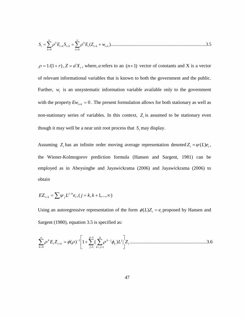
47
5.3...............................................................................).........(00
ktktt
k
k
ktkt
k
k
t wZESES
)1/(1 r , tXaZ , where, a refers to an )1( n vector of constants and X is a vector
of relevant informational variables that is known to both the government and the public.
Further, tw is an unsystematic information variable available only to the government
with the property 0ktEw . The present formulation allows for both stationary as well as
non-stationary series of variables. In this context, tZ is assumed to be stationary even
though it may well be a near unit root process that tS may display.
Assuming tZ has an infinite order moving average representation denoted tt eLZ )( ,
the Wiener-Kolmogorov prediction formula (Hansen and Sargent, 1981) can be
employed as in Abeysinghe and Jayawickrama (2006) and Jayawickrama (2006) to
obtain
Using an autoregressive representation of the form tt eZL )( proposed by Hansen and
Sargent (1980), equation 3.5 is specified as:
6.3................................................................)(1)(1
1 1
1
0
t
p
j
p
jk
j
k
jk
kt
k
t
k ZLZE
),...,1,(,
kkjeLEZ t
kj
jkt

48
Given that there is no interest in the nonlinear parameter, 3.6 is re-specified as:
7.3.......................................................................................1
1
0
0
t
p
j
j
jkt
k
t
k ZLZE
Recall condition 3.4 in the definition of the PVBC which states that )0lim(
NttN
BE . Thus,
replacing tt XaZ and redefining the respective parameters, it is possible to write;
8.3....................................................................................................1
1
1
tit
p
i
it XD
Note that although equation 3.8 and 3.4 which is the present value borrowing constraint
(PVBC) might not be different, the present formulation disaggregates the components of
the budget surplus to allow a larger information set in explaining the debt equation.
However, with the standard definition of the budget surplus, this formulation can easily
be adopted to explain the relationship between public debt, tax revenue and government
expenditure. Further in equation 3.8, t is assumed to be a well behaved stochastic
disturbance term.
For purposes of understanding the relationship between public debt, tax revenue and
government expenditure, a VECM framework was more appropriate. The VECM was
specified as:
9.3.................................................................................,
1
1
'
t
p
i
itijtt WWVW

49
The first component is the error correction components in levels while the second
component on the RHS of equation 3.9 is the VAR component in first differences. Wt is a
vector of variables. Γ matrix captures the short-term adjustments among the variables at
the ith lag. β' is the matrix of cointegrating vectors and is the speed of adjustment
parameters. The elements of the matrix relate also to the weak exogeneity. j is the lag
structure. V is a vector of constants and t is a vector of white noise error terms.
3.4 Definition and Measurement of Variables
Public debt is total outstanding borrowing by the government less currency. Public debt
was measured in Kenyan shillings.
Tax revenue is total government income due to taxation. Tax revenue was measured in
Kenyan shillings.
Government expenditure is total money spend by the government less interest payments.
Government expenditure was measured in Kenyan shillings.
3.5 Data Type, Source and Refinement
This study utilized annual time series data over 1960 ─ 2011, for Kenya. Data was
obtained from economic surveys from 1960-2013. Because the data was available in
fiscal years, it was converted to calendar years by splicing. Splicing involves constructing
a long time series of economic variables through piecing/linking together short
heterogeneous series (Fuente, 2013). To obtain data in calendar years, those observations
that were in fiscal years were averaged.
50
All variables were converted into their real values through dividing their respective
nominal values by the consumer price index (CPI). Use of the CPI was justified because
the variables estimated fell on the expenditure side of the economy.
3.6 Stationarity Analysis
This study employed time series data, for 1960-2011 in Kenya. With such kind of data, it
was necessary to determine the properties of the series to ensure they are stationary and
therefore integrated order zero I (0), to avoid estimation bias (Yule, 1926; Granger and
Newbold, 1974; Banerjee et al., 1993).
The first step was therefore to determine the nature of stationarity and integration in the
series to be tested. This is because most time series are non-stationary (have unit roots). It
becomes essential to test for unit roots since their presence would lead to spurious and
inconsistent estimates so that the mean and variance are time dependent hence would
explode with time (Russel and Mackinnon, 1993; Bohn, 2005; Freedman, 2007).
Spurious model is when an unrelated series gives model estimates that are statistically
significant with high R-squared. This affects inference as parameter estimates are
meaningless. On the other hand, inconsistent estimation is when the regressed and
regressors have different orders of integration. In this scenario, inference would not be
valid since the variance was time dependent. To avoid these problems, it was necessary to
establish presence or absence of unit roots.

51
This study used the Augmented Dickey Fuller (ADF) (1979) and the Philips and Perron
(1988) unit root tests. The inclusion of the Philips Perron (PP) test stemmed from the
argument that in the presence of unusual circumstances, the conventional ADF unit root
test would be invalid (Pierre, 1989; Sjo, 2008), for example if a series has an explosive
unit root (Suresh et al., 1999). In addition, the PP unit root test is particularly robust on
any heteroscedasticity in the error term and the user also does not need to specify a lag
length (Rothe and Sibbertsen, 2005).
3.7 Cointegration Analysis
The next step was to test the order of integration to determine equilibrium relationships
for the series which individually may not be in equilibrium. This involves testing for both
short and long run equilibrium. Presence of co-integration also leads to spurious results
and wrong interpretation; and is necessary to test (Nelson and Plosser, 1982; Dolado,
Gonzalo and Marmol, 1999). Since the Engle and Granger (1987) co-integration
technique would be invalid because more than two variables were being analysed, the
Johansen and Juselius (1990) test was used. Engle and Granger showed that if variables
have unit roots (they are not stationary and integrated of order one ))1((I before the first
difference, and become stationary after the first difference, there exists a long run
relationship between the variables at level (before first difference). This also indicates
that unidirectional or bidirectional causality must be present in at least the integrated
order zero ))0((I series/variables.

52
In the first step of the Engle and Granger co-integration technique, unit root tests was
done to show order of integration for the variables of interest.
10.3.......................................................................................................................110 ttt xaay
11.3.......................................................................................................................210 ttt yaax
In step two, the residuals are tested to find if they are stationary using unit root tests such
as Dickey Fuller. One shortcoming of this two-step test is that an error in the first step
affects the second step results badly (Shah and Ali, 2012). This problem is overcome by
the Johansen and Juselius (1990).
Johansen and Julius co-integration technique involves maximum likelihood estimation
(MLE) of the reduced rank model. It is done by estimating an unrestricted Vector
autoregression (VAR) model stretching to p lags to find the underlying lag structure of
the data, as shown:
In the first step, an autoregressive process of order p (AR (p)), is specified as:
12.3..............................................................................,..., 1111 tptptptt eyyyy
∆ shows variables that have been differenced and are therefore integrated order
zero ))0((I , is a constant, ty and te are )1( n vector of variables and vector of
innovations, respectively. In effect, this is a reduced form equation and each variable in

53
ty has the potential of being regressed on its previous values as well as those of other
variables (Hinaunye and Mbazima, 2008).
Assuming there exists co-integration of order p, this equation can be rewritten by
replacing ∏=αβI, where ∏ = IA
p
i
i 1
= ),...,( pi AAI , is a vector that shows
long run coefficients of a matrix and are really useful in this test. Ai, i =1,…,p, while I is
an identity matrix. Replacing ∏, 3.12 is then written as:
13.3...........................................................................,..., 1111 tptptptt eyyyy
As mentioned, is important in capturing the long adjustments to changes
in ty and defined with asymptotically efficient estimates of and that this test is
assumed to give, both which are of dimension )( pn . The term shows the pace/speed
that adjustment from disequilibrium occurs while represents co-integrating vectors and
are charged with facilitating ty attains its long run equilibrium/steady state. Equation
3.12 can be simplified as:
14.3..............................................................................................1
tititi
ip
i
t eyyy
So that i = 1,...,1),,...,( 1
1
piAAIA i
p
ij
i , where i captures the short run
adjustments to the changes in ty , and te is a vector of error terms/residuals and

54
represents those factors the variables considered here do not capture or rather these are
impacts from exogenous shocks.
Therefore, when the rank of matrix equals r , co-integration exists. The rank can either
be a full rank, reduced rank or zero. A full rank is equivalent to rank, nr where there
exists n co-integrating equations and all variables integrated order zero ))0((I . A reduced
rank means there are 1n co-integrating variables and the most appropriate method is to
utilize error correction mechanism (ECM). Rank equal zero, shows that all elements in
are zero and there is no co-integration so that estimation is done at the first difference
without any long run elements. The co-integrating rank is tested using the trace test and
the maximum eigenvalue test.
3.8 Distribution and other Diagnostic Tests
A number of tests were carried out on the regression residuals to ascertain whether the
VECM was well specified. Eigenvalue stability test to check whether the number of
cointegrating equations was well specified, LM test for serial correlation in the residuals
and Jargue-Bera test for normally distributed errors were carried out. The stationarity of
the cointegrating equations was checked by plotting the predicted cointegrating equations
over time and studying their behaviour. This is because the inference on the parameters
of the adjustment parameters depends on the stationarity of the cointegrating equations.
55
3.9 Data Analysis
This section deals with how the data was processed and used to achieve the objectives of
the study. Before the processing of the data, the data was summarized into descriptive
statistics where measures of central tendency and dispersion such as the mean, maximum
and minimum were presented. The data analysis was mainly based on quantitative
econometric techniques presented in the subsections below.
3.9.1 Correlation Analysis
In examining the relationship between public debt, tax revenue and government
expenditure this study employed correlation analysis. Correlation was measured by the
correlation coefficient denoted as r for a sample and it shows the kind/type and strength
of association exhibited by variables. Although various methods and formulae that
compute correlation exist, all of them yield the same result and therefore the outcome is
independent of the method.
This study used the Pearson product moment correlation coefficient (PPMCC) in
examining the relationship between public debt, tax revenue and government
expenditure. The Pearson product moment correlation coefficient (PPMCC) is named
after Karl Pearson (1900) and is based on a number of assumptions. First, the relationship
between variables studied is linear. This is because interest remains explicitly on linear
correlation so that in the event of a curvilinear relationship, the Pearson product moment
correlation coefficient (PPMCC) underestimates the whole relation. Second, the scale in
which the variables are measured is either interval or ratio scale and needs paired

56
observations. Otherwise if the scale is for instance ordinal or any other, this test fails.
Third, use of Pearson product moment correlation coefficient (PPMCC) requires a normal
distribution with constant variance (homoscedastic), as you move along the line of best
fit. Fourth, in the effect that there is presence of outliers then they should be removed or
be kept at their minimum levels so that they do not affect outcome. Outliers are
observations completely different from the overall data either too small or too large or
just too distinct that they may have huge effects on best fit and correlation and lead to
very different conclusions.
Upon satisfaction of the above assumptions, the Pearson product moment correlation
coefficient (PPMCC) was computed as follows:
15.3..................................................................
)()()()(
))((
2222
yynxxn
yxxynr
Where n is the sample size or the number of ordered pairs, while x and y are variables
based on which correlation is computed.
Before computing the correlation coefficient it is always good practice to generate/plot a
scatter diagram in the first step. A scatter diagram/plot shows how the data points fits to
the line of best fit and gives a general idea of how data resembles a line. However this is
not to be relied on since the eye sometimes and many times is not a good judge and may
mislead. So the next step is basically to compute the Pearson product moment correlation

57
coefficient (PPMCC). Hypothesis tested was the null hypothesis that there was no
correlation, 0:0 rH against the alternative hypothesis indicating presence of
correlation, 0:1 rH
After computing the Pearson product moment correlation coefficient (PPMCC), the
direction of a relationship is shown by the sign accompanying the correlation coefficient.
A positive sign )0( r showed that variables move together. For example, when one
increases, the other variable too also increases. On the other hand, a negative sign )0( r
showed that the two variables move in different directions, an increase in one variable
causes the other variable to decrease, and the converse is true. The strength of the
correlation was shown by the absolute value of the correlation coefficient )(r . Where,
3.01.0 r showed a small/weak relation, 5.03.0 r displayed medium/moderate
relation while 0.15.0 r showed a large/strong relationship between variables.
3.9.2 Vector Error Correction Model
The presence of cointegration meant that the variables were related by a Vector Error
Correction Model (VECM). While the VECM measures the short run dynamics,
cointegration shows long run relationships. The parameters of interest in the VECM were
the coefficients on the speed of adjustment parameters and the beta coefficients.

58
3.9.3 Granger Causality
Series that have an error correction representation point to the existence of causal
relationships among variables. This study performed causality analysis in the spirit of
Granger to examine the relationship between tax revenue and government expenditure.
Granger causality analysis is based on the criteria that past and present information
determines the future better (Granger, 1969). That is, variable y causes variable x if past
values of y and x predict x better rather than previous values of x alone (Granger, 1969).
Similarly, x causes y if past values of x and y predict x better rather than previous values
of y alone.
Based on the objectives of the study, granger causality was examined between public
debt and tax revenue and public debt and government expenditure. Formulation of
Granger causality tests for two variables x and y are written as:
16.3..............................................................................................2
1
1
1
tit
n
i
iit
n
i
it ybxax
17.3.......................................................................................4
1
3
1
tit
n
i
iit
n
i
it xdycy
x and y are the series to be tested, ,3,2,1; ini are maximum lag lengths determined
using Akaike Information Criteria (AIC) (1969) and Schwartz information criteria (1978)

59
where the lag length that is minimum in either case is taken. Error terms t( and )t are
assumed uncorrelated, that is, the expectation of their means is zero )0),(( ttE .
Hypotheses to be tested in equation 3.16 are H0: y does not granger cause x against H1: x
granger causes y, while in equation 3.17, hypotheses to be tested are H0: x does not
granger cause y against H1: y granger causes x.
In effect that the series is integrated of order one, I (1) and hence co-integrated,
traditional granger test which is based on the F test does not have a standard distribution
and causality is examined within Error correction mechanism (ECM), as shown below;
18.3..................................................................111
1
1
2
1
1 tt
n
i
n
i
itiitit vybxax
19.3..................................................................122
3
1
4
1
1 tt
n
i
n
i
itiitit ydxcy
Where 11 t and 12 t represent lagged error terms from equation 3.16 and 3.17 while 1
and 2 show adjustment of y and x to long run equilibrium.
3.9.4 Impulse Response Functions
Impulse response functions aid in examination of whether exogenous shocks have a
positive or negative effect on the other variable in the system, or how long it will take for
the effect of that variable to work through the system (Brooks, 2002; Mpofu, 2009). This

60
study employed Cholesky’s Forecast Error Variance Decomposition (FEVD) procedure.
Based on the objectives of the study the response of public debt to exogenous shocks
from the tax revenue and government expenditure side was examined. The results for
FEVD were examined and interpreted with the aid of graphs and tables.
3.9.5 Forecasting
VECMs that display cointegration produce forecasts with variables both at levels and at
first difference. In this study, two types of forecasts were computed. These were the
dynamic forecasts and the out of sample forecast. Dynamic forecasts were used to
compare the predicted values to those observed in the study period. In comparison, the
out-of-sample forecast was used to compare the growth of the width of the confidence
interval to the forecast period.

61
CHAPTER FOUR
EMPIRICAL FINDINGS
4.1 Introduction
This chapter deals with the empirical findings of the study. Findings of time series
properties, post diagnostic tests and the regression results including those of correlation
are presented and discussed.
4.2 Descriptive Statistics
The sample consisted 52 observations over 1960-2011. Table A1 in the appendix presents
the descriptive statistics. The level of public debt in magnitude remained higher than for
the respective variables of tax revenue and government expenditure. This was particularly
evident from the year 1994 towards the end of the study period. This was supported by
both the mean and the dispersion (standard deviation). The converse was true for the tax
revenue variable which had a mean and standard deviation of KES 103824.7 million and
KES 160399.1 million, respectively. A graphical representation showing the trend in the
series over the study period is found in figure 1A in the appendix.
Drastic movements were evident in the data. Most movements were associated with
either years which had had general elections or those years around the elections. For
public debt particularly, drastic movements were evident between 1977 and 1978, where

62
public debt rose in the range of 5%. Between 1991 and 1992, there was a sharp decline in
public debt with the level going flat into 1993. Perhaps this could be once again attributed
to election cycles or either aid freezes or structural adjustment programs (SAPs).
Thereafter, although public debt assumed an upward trajectory, there was evidence of
moderate fluctuation type growth between: 1995-1996; 2000-2001; and 2005-2006.
Prior to 1980, even though the curve for government expenditure widened at a faster rate
than that for tax revenue, both curves remained smooth without those movements that
captured attention. There was a sharp increase in both tax revenue and government
expenditure in 1994. The growth in tax revenue moderated into 1996 but that in
government expenditure persisted two years on. No much activity can be reported for the
tax revenue curve for the remainder of the study period except an upward trajectory. For
government expenditure, however, a decline of about 58% - also the highest in the study
period was recorded over 1998-1999. Nonetheless, growth in the variable picked up a
year later but a little lower than the decline. At the end of the study period, the levels of
all variables were higher compared to those over the whole study period.
An interesting trend in the study period was that the rate of growth in public debt was
lowest in comparison to the other two variables (tax revenue and government
expenditure) and about two times lower than that in government expenditure. This would
imply that although the growth in public debt is being seen as alarming, it reflects fast
growth in government expenditure outpacing the growth in tax revenue. It might well

63
reflect the narrow tax base in the economy or inefficiencies in tax administration
characterised by tax evasion. On this basis therefore, the budget deficit has to be financed
by further accumulation of public debt.
4.3 Findings for Stationarity Analysis
To determine the underlying orders of integration for public debt, tax revenue and
government expenditure series, the Augmented Dickey Fuller (ADF) and Philips Perron
(PP) unit root tests were conducted. The results for the ADF and the PP unit root tests
are reported in table A2 in the appendix. For the ADF unit root test, four lags were
selected based on the Akaike Information Criterions’ minimum value. 1 per cent level of
significance was used. The ADF unit root test indicated that with an intercept only, public
debt was the only variable that was non stationary at level. At first difference, the series
for public debt remained non stationary that could question the lag selection procedure
Contrary to the case for intercept, all the series under study were non stationary at levels
when considered with trend. At first difference (with the exception of the tax revenue
series) most series became stationary. This meant that with the trend, public debt and
government expenditure were integrated order one or, were each I (1).
The results for the ADF unit root tests needed deeper insight. This could point to a
problem in the lag selection procedure. And because of this, it was justified to proceed
and test these series for their orders of integration using the PP unit root test. This was
especially so in light of the argument put forward by Pierre (1989) and Sjo (2008) that in

64
the presence of unusual circumstances the conventional ADF unit root test would be
invalid, for example in the presence of an explosive unit root (Suresh et al., 1999). Also,
the PP unit root test is reported to be particularly robust to any heteroscedasticity in the
error term. Moreover, the user does not need to specify the number of lags (Rothe and
Sibbertsen, 2005) for this test. The Newey – West selected three lags For the PP unit root
test with default lags. With this justification, it was fit to present the results for the PP
unit root test reported in table A2 in the appendix. For all cases, none of the variables
were stationary at levels. They, were however stationary or I (0) at first difference. This
meant they all had one unit root each.
4.4 Findings for Cointegration Analysis
As all variables were integrated of order one (I(1)), ordinary estimation techniques were
going to be invalid due to the existence of one or more equilibrium relationships among
them. Given the fact that also more than two variables were being analysed, the Engle
and Granger test of cointegration was in practice invalid. To estimate what and how
many equilibrium relationships existed, this study adopted the Johansen and Juselius
(1988, 1995) cointegration technique. Results for the Johansen cointegration test are
presented in table A3 in the appendix. Three lags were selected for the test. The AIC lag
selection criterion was used as it yielded minimum value (68.77). 1 percent level of
significance was used. Both the trace and the maximum eigenvalue test statistics
indicated two cointegrating equations.
65
4.5 Distribution and other Diagnostic Test Results
Before accepting the results for the specification, it was necessary to test the significance
of the model. The tests conducted included the VECM stability test, the LM test for serial
correlation and the Jargue Bera test for whether the residuals came from a sample that
followed normal distribution. The results for the VECM stability test are presented in
table A4 in the appendix. The eigenvalue stability condition in the VECM showed that
the eigenvalues of the companion matrix were inside the unit circle, and the real roots
were far from one (1). This was in support of the view that the number cointegrating
equations in VECM was well specified.
The langrange multiplier (LM) test was used to test presence of serial correlation. The
langrange multiplier (LM) test for autocorrelation on the residuals of order five indicated
that at 1 percent level of significance, the null hypothesis of serial correlation could not
be rejected. All p-values were lower than the 0.01 rejection level. Following Achen
(2000) and Keele and Kelly (2006), who noted that serial correlation could be eliminated
by inclusion of additional lags, more lags were added in an effort to eliminate serial
correlation. However this was insignificant as it was only at lag six that serial correlation
hypothesis could be rejected when the order of the LM test was increased to six. These
results were not presented as they were insignificant.

66
The study proceeded to test the residuals for normal distribution. The Jargue-Bera test
(Jargue Bera, 1981) was used. The null hypothesis that the residuals followed normal
distribution was tested against the alternative that the residuals were not normally
distributed. The results indicated that the null hypothesis of normally distributed residuals
was rejected at 1 percent level of significance. This could be attributed to high
fluctuations in the data in the calendar years of 1992, 1999, 2002, 2006, 2008 and 2009.
These results are not reported.
The errors from the cointegrating relationships were plotted to establish how they
behaved. The plots are presented in figure A2 in the appendix. The plots revealed that the
errors fluctuated around zero prior to 2000. The errors from the first cointegrating
equation assumed a negative trend form 2001 and never returned to zero. For the second
cointegrating equation, the errors decline from 2001 to between 2002 and 2003 where
they assume an upward trend. The trend however reverts, with the errors declining further
before showing a slight increase into the end of the study period.
4.6 Regression results
Having conducted these diagnostic tests in the study, the estimation results on the
relationship between public debt, tax revenue and government expenditure are presented.
Results for VECM are reported in table 4.1.

67
Table 4.1: Results for Vector Error Correction Model (VECM)
Coefficients Dependent variables
Public Debt Tax Revenue Government Expenditure
Adjustment Parameters, s
1 -0.3576* (0.01) -0.0749* (0.01) -0.3615* (0.01)
2 4.5635** (0.02) -0.2322 (0.58) 4.0368* (0.00)
P-values are in parentheses. An asterisk denotes a coefficient is statistically significant at 1 percent level of
significance. Double indicates a coefficient is statistically significant at 5% level of significance. All values
reported were rounded to four decimal places. Five lags (similar to what was used in the Johansen
cointegration test) were selected based on the AIC (Akaike, 1974) value of 66.97.
All coefficients on the first speed of adjustment parameter ( 1 ) were negative (as
expected) and less than one. Moreover, the coefficients were all statistically significant at
either 1 or 5 percent levels of significance. This implies that deviations from the long run
equilibrium are corrected in the next year by the size of the coefficient. For the public
debt equation, about 36% of these deviations are corrected in the next period. The first
speed of adjustment coefficient for the tax revenue equation was however low implying
slow adjustment to the long run equilibrium. The coefficients in the first cointegrating
equation indicated equilibrium relationships between public debt and government
expenditure. The coefficients in the second cointegrating equation pointed to
equilibrium relations between tax revenue and government expenditure which could
possibly be the budget deficit relation.
The short run variations in the VECM model were examined. Results for the short run
VECM model are presented in table 4.2.

68
Table 4.2: Results for VECM Short run model
Public Debt Tax Revenue Government
Expenditure
First lag of public debt 0.67* (0.00) 0.14 (0.00) 0.16 (0.11)
Second lag of public debt -0.42 (0.06) -0.01 (0.82) 0.21** (0.05)
Third lag of public debt 0.28 (0.19) -0.08 (0.08) 0.06 (0.60)
Fourth lag of public debt 0.01 (0.96) -0.14* (0.02) 0.28** (0.03)
First lag of tax revenue -5.14* (0.00) -0.78** (0.02) -2.44* (0.00)
Second lag of tax revenue -3.09** (0.02) -0.45 (0.11) -2.13* (0.00)
Third lag of tax revenue -1.67 (0.12) 0.45** (0.04) -0.13 (0.80)
Fourth lag of tax revenue -2.99* (0.01) -0.58* (0.02) -2.57** (0.00)
First lag of government expenditure 2.48** (0.03) -0.22 (0.36) 0.99 (0.08)
Second lag of government expenditure 2.30* (0.01) 0.02 (0.94) 0.76 (0.10)
Third lag of government expenditure 1.50** (0.02) 0.13 (0.35) 0.35 (0.25)
Fourth lag of government expenditure 0.80** (0.03) 0.08 (0.30) -0.12 (0.51)
F-statistic 4.72* (0.00) 2.19 (0.09) 6.22* (0.00)
R-squared 0.74 0.94 0.88
D-Watson 1.54 1.63 1.98
P-values are in parentheses. An asterisk indicates a coefficient is statistically significant at 1 percent level of
significance. Double asterisk indicates a coefficient is statistically significant at 5% level of significance.
Results of table 4.2 indicate that the model explains 74% of the variations in public debt.
Variation in public debt is influenced by its own first lag as well as most lags of tax
revenue and government expenditure. In the public debt equation the coefficients on most
lag terms of public debt, tax revenue or government expenditure is statistically significant
at either 1% or 5% level of significance.
69
Series that have error correction representation point to the existence of causal
relationships. This justified examination of granger causality tests among the variables.
Granger causality was examined between: public debt and tax revenue; public debt and
government expenditure, and; tax revenue and government expenditure. Granger
causality between tax revenue and government expenditure was justified on account that
it would be useful in devising an optimal strategy for budget deficit reduction. Moreover,
the strategy for public debt reduction depends on the strategy for budget deficit reduction.
Recall that unit root tests indicated each of the series was I (1), pointing to possible long
run equilibrium relationships among these series. The Johansen test for cointegration
assuming four lags based on the AIC and 1 percent level of significance indicated 1
cointegrating equation in each of the three hypotheses tested - supporting existence of
long run association. Given this outcome, in testing causality the traditional granger
causality test based on the F test does not have a standard distribution and causality was
examined on an error correction model (ECM). Three lags were used in estimating all
ECM equations (except in testing causality between tax revenue and government
expenditure where four lags were used). Results for granger causality are presented in
table A5 in the appendix.
Results for table A5 indicated bidirectional flow between: public debt and tax revenue
and; public debt and government expenditure in the long run. Between tax revenue and
government expenditure, however, there was evidence of unidirectional flow running
from government expenditure to tax revenue at 1% level of significance. The results

70
indicated that government expenditure granger causes tax revenue both in the short and
long run. This finding is in line with the findings of Carneiro, Faria and Barry (2005),
Raju (2008), Wahd (2008) and Zapf and Payne (2009). They are however in contrast to
the findings by Ghartey (2008) and Ghartey (2012) in favor of the revenue-spend
hypothesis. However, and as noted also by Garcia (2012), several factors account for
divergent results ― statistical techniques, method approaches, reporting periods, and the
level of aggregation. The optimal strategy for deficit reduction hence is a cut on
government expenditure to restore fiscal discipline.
Next was to conduct impulse response functions (IRF) analysis. Impulse response
functions indicate how a system would respond to exogenous shocks. For the IRF,
however, there’s controversy as to whether the series in a VAR need to be stationary.
Those against differencing argue in favor of loss of significant information related to co-
movements in data. The study adopted the Cholesky forecast error variance
decomposition (FEVD) procedure. 11 steps (years) were used. The graphical
representation of the results for FEVD is presented in figures A3 through A7 in the
appendix. The graphs were important in establishing the whether the response to shocks
was positive or negative. Generally, exogenous shocks to tax revenue and government
expenditure have a permanent effect on public debt.
From the graphs for the IRFs, public debt responded positively to the innovations in both
tax revenue and government expenditure. In the short run, however, the response is very
71
minimal but is evident in the long run. A detailed interpretation is discussed under table
4.3. Similarly, response of public debt to government expenditure shocks is neutral at
first (in year three to four). Thereafter public debt responds positively to exogenous
shocks in government expenditure. Finally, public debt responds positively to its own
shocks up to about year one (short run). Thereafter the effect of a shock is negative into
the long run.
The tabular representation of the results for the FEVD is reported in table 4.3. The results
of the FEVD analysis based on the VECM provide much useful information on the
evolution of the public debt, tax revenue and government expenditure-relationship in
Kenya over time.
Generally, public debt seems to have had a highly dominant position in the Kenyan
public finance system. Over the whole sample period the forecast error variance of the
public debt is almost completely attributable to exogenous shocks from the public debt
side, both in the short and the long-run.

72
Table 4.3: Results for Forecast Error Variance Decomposition (FEVD)
Step impulse = gr imp = ge imp = pd imp = pd impulse = pd
response = pd res = pd res = gr res = ge response = pd
0 0 0 0 0 0
1 0 0 0.288 0.001 1
2 0.004 2.4e-06 0.262 0.002 0.996
3 0.006 0.002 0.152 0.015 0.992
4 0.017 0.012 0.109 0.014 0.972
5 0.033 0.017 0.317 0.180 0.949
6 0.035 0.029 0.301 0.291 0.936
7 0.104 0.027 0.302 0.309 0.870
8 0.158 0.035 0.437 0.423 0.807
9 0.347 0.035 0.356 0.316 0.618
10 0.426 0.045 0.381 0.387 0.529
11 0.441 0.047 0.431 0.460 0.512
Key: pd-public debt gr-tax revenue ge-government expenditure
Innovations in both tax revenue and government expenditure do not explain the forecast
error variance in public debt up to year two. From the third year however; public debt
responds positively by 1 % to exogenous shocks on tax revenue. In the long run, about
35% to 44% of the increase in forecast error variance in public debt is explained by the
exogenous shocks to tax revenue. For government expenditure, its innovations are at first
neutral to the variance in public debt. In the long term, the eleventh year, 5 % of the
variance in public debt, is explained by the shocks to government expenditure.

73
Tax revenue responds positively to exogenous shocks to public debt in the short run and
the long run. Innovations in public debt explain 29% and 26% of the forecast error
variance in tax revenue in the first and the second years respectively. In years three and
four, innovations in public debt explain about 15% and 11% of the variance in tax
revenue respectively. In the long run, innovations in public debt explain about 44% of the
variance in tax revenue-in the eighth year. Similarly, innovations in public debt explain
the forecast error variance of government expenditure in the long run. An exogenous
shock on public debt explains 39% and 46% of the forecast error variance in government
expenditure in years ten and eleven, respectively. Innovations in public debt explain
100% of its own forecast error variance in the short term. In the long term it explains
about 51% of its own variance. Results for FEVD support the results for granger
causality analysis.
After interpreting results for FEVD, dynamic forecasts were done. The results for the
dynamic forecasts are presented in figure A8 found in the appendix. The levels for tax
revenue and government expenditure predicted by the model were slightly lower than that
observed throughout the sample period, 2001-2011. There was however an exception in
the year 2006 when the forecasted figure was above that observed. In the case of public
debt, the predicted figure was equal to the observed figure over 2004-2006, otherwise the
predicted values were above those observed in most years.

74
The out of sample forecast was then computed. The out-of-sample forecast for 2011
through 2030 is presented in figure A9 in the appendix. The width for the confidence
interval increased with the forecast period, as was expected. The forecasts pointed to
continued growth in these variables.
4.6.1 The relationship between public debt and government expenditure
Results for correlation analysis showed strong positive association between public debt
and government expenditure. The correlation coefficient was statistically significant at 1
percent level of significance. This meant that a decrease (increase) in government
expenditure would lead to a decrease (increase) in public debt which supported the
findings of Bilbiie, Meier and Mueller (2008). This would particularly represent
decreased (increased) reliance on borrowing (public debt) in budget deficit finance.
Granger causality analysis supported feedback effect between public debt and
government expenditure in the long run. The coefficient on the ECT was statistically
significant at 1 percent level of significance.
Public debt responds positively to exogenous shocks in government expenditure in the
long run. This finding coincides with findings of Kanano (2006), Cassimon and
Campenhout (2007), Nyamongo and Schoeman (2007) and Bilbiie, Meier and Mueller
(2008). However, it contrasts with results of Shonchoy (2010) and Stegarescu (2013). In
particular, Stegarescu (2013) found out that larger shares of government expenditure
were associated with lower debt. This point to the usefulness of including socioeconomic

75
as well as political factors as they play a huge role in the overall levels of these variables.
Nonetheless, this study agrees that the level of total expenditure has a debt increasing
effect, which is in line with the finding of this study.
4.6.2 The relationship between public debt and tax revenue
Results for correlation analysis showed strong positive association between public debt
and tax revenue. The correlation coefficient was statistically significant at 1 percent level
of significance. The results of correlation between public debt and tax revenue were
desirable. If public debt increased, tax revenue would also increase. This emphasised the
economic argument of no direct link between public debt and government revenue but
through the deficit channel. Public debt only represents a means to budget deficit finance.
For public debt to increase there must be evidence of widening in the budget deficit (fast
growth in government expenditure outpacing the response in revenue). In this case, fiscal
authorities would increase the tax rate to finance deficits. In turn, tax revenues would
increase.
Granger causality analysis supported feedback effect between public debt and tax
revenue in the long run. The ECT coefficient was statistically significant at 1 percent
level of significance.
Public debt responds positively to exogenous shocks in tax revenue over the long run.
This supports studies by Shonchoy (2010) and Greiner, Koller and Semmler (2011).
Particularly, for real world economies the degree of public debt service necessitates a

76
means to finance it. For developing nations like Kenya, public debt burden may not have
a direct impact on government expenditure. Resort to taxation as a means to finance the
public debt burden is fast and more appropriate compared to cutting pre-planned
government expenditure.

77
CHAPTER FIVE
SUMMARY, CONCLUSIONS AND POLICY IMPLICATIONS
5.1 Introduction
This chapter presents the summary, conclusions and the policy insights stemming from
the study. The limitations that the study encountered are also presented. Finally,
recommendations about further study are presented towards the end of the chapter.
5.2 Summary
The study sought to understand the relationship between public debt, tax revenue and
government expenditure in Kenya over the sample period 1960-2011. The specific
objectives in the study were the relationship between public debt and tax revenue and the
relationship between public debt and government expenditure. This was inspired by the
growing levels of budget deficits and public debt. The theoretical framework of the
present value borrowing constraint was adopted in the study. Time series data was used
over the sample period. Data for public debt less currency, tax revenue and government
expenditure excluding interest payments were all measured in million Kenyan shillings.
Data was obtained from the KNBS publication of the Economic Survey over 1960-2013.
All variables were divided by the CPI to convert them from their nominal values into
their real values. ADF unit root and the PP unit root tests were employed to determine the
orders of integration in the series. After ascertaining that all the series in the study were
integrated of order one or I(1) pointing to the possibility of long run equilibrium

78
relationships, the Johansen and Juselius cointegration technique based on both the trace
statistic and the maximum eigenvalue statistic was used to test for the long run
equilibrium relationships. The results for cointegration based on both statistics indicated
two cointegrating relationships.
The study then proceeded to use the VECM since ordinary estimation techniques were
invalid due to cointegration. The tests conducted to test the significance of the model
included the VECM stability test, the LM test for serial correlation, and the Jargue Bera
test for normality in the residuals. As required in the VECM literature, the components of
the VECM including results for impulse response functions (IRF) employing the
Cholesky forecast-error variance decomposition (FEVD) and the dynamic forecasts were
also evaluated. Correlation between the variables was finally investigated.
5.3 Conclusions
This study sought to understand the relationship between public debt, tax revenue and
government expenditure over 1960-2011. Given the empirical findings, the study
concludes that public debt responds to both tax revenue and government expenditure.
The first objective was to understand the relationship between public debt and
government expenditure. The study concludes that public debt responds positively to
shocks from the government expenditure side particularly over the long run. In addition,
bi-directional causality exists between public debt and government expenditure.
79
Furthermore, results for correlation indicated strong positive association between public
debt and government expenditure.
The second objective was to understand the relationship between public debt and tax
revenue. The study concludes that public debt responds to tax revenue. In the short run
model, public debt responds negatively to a change in tax revenue and the coefficient is
statistically significant. Public debt responds positively to shocks on tax revenue
particularly over the long run. Evidence of response in the long run could mean there are
gaps in the implementation of government fiscal policies in the economy since such
policies take time to filter through the economy. In addition, bi-directional causality
exists between public debt and tax revenue. Furthermore, results for correlation also
indicated strong positive association between public debt and tax revenue. This meant
that government policy can affect the tax base to influence the level of public debt
because a change in tax revenue would cause a more than proportionate change in public
debt.
The government follows the spend-revenue hypothesis in its budget deficit decisions.
This means government spends first before raising revenue sources. This could be so
given multiple sources of revenue at the disposal of the government. Given the levels of
the budget deficit and public debt, a cut in government expenditure is necessary to restore
fiscal discipline as well as solve the budget deficit and public debt problems.

80
5.4 Contribution to Knowledge
First, this study explored the relationship between public debt, tax revenue and
government expenditure between 1960 and 2011. This study has shown that
understanding the relationship between public debt, tax revenue and government
expenditure is important if any policy decisions on solving the budget deficit and public
debt have to be reached. Also, the study has established that public debt, tax revenue and
government expenditure move closely together such that any policy decision should be
designed in such a manner that it affects the variables together.
This study has established that spend-revenue hypothesis between tax revenue and
government expenditure is supported in Kenya. This contrasts the study done by Ghartey
(2008) which supported the revenue-spend hypothesis.
5.5 Policy Implications
To reduce public debt, fiscal authorities should enhance measures that increase tax
revenues. These include sealing tax loopholes for example tax evasion. This is because
negative and statistically significant coefficients were found on most lagged terms of tax
revenue in the short run VECM model. This means a KES 1 million increase in tax
revenue leads to a decline in public debt in the range of KES 3 million and KES 5 million
in the short run.

81
Fiscal discipline and fiscal consolidation is necessary in the wake of the levels of budget
deficits and public debt. This can be achieved by prioritising expenditure on key sectors
that have the potential of boosting the overall productivity of the economy in the long
run. This study found that the coefficients of government expenditure that explained
public debt in the short run VECM model were positive and statistically significant. A cut
of KES 1 million in government expenditure leads to a decline in public debt of between
KES 1 million and KES 2.5 million. In addition, in the long run public debt responds
positively to positive shocks from the government expenditure side. Moreover, the results
for correlation showed that a 1% cut on government expenditure translates to a 52%
decline in public debt.
5.6 Limitations and Areas for Further Research
This study encountered a number of limitations. First, to the best of the author’s
knowledge no study in the past had attempted to explore the relationship between public
debt, tax revenue and government expenditure. As a new study therefore, getting
previous literature on the subject was a big problem. The study however relied on those
studies that were as close as possible to the subject.
The study utilised time series data. Data available at the Kenya national bureau of
statistics (KNBS) publication of the economic survey was in fiscal years. Splicing which
involved piecing/linking together short heterogeneous series was relied upon.

82
Since any study is inconclusive, a number of observations about further research are
therefore in line. First, the residuals in the VECM estimates depicted high serial
correlation as well as non normality. To be able to justify the significance of this model,
this study recommends that future research deal with this issue.
Second, this study used the theoretical framework of the present value borrowing
constraint (PVBC) credited to Hamilton and Flavin (1986). However, it did not test this
hypothesis, to establish whether government follows the present PVBC. Future studies
should thus seek to establish whether this constraint holds in Kenya, given that to the best
of the author’s knowledge, no single study has taken this direction.
Third, most econometric techniques give different results. Future studies should attempt
to explore the relationship between public debt, tax revenue and government expenditure
using other techniques such as Generalised Least Squares (GLS) or Generalised Method
of Moments (GMM).
Fourth, devolution is so far under implementation. Government expenditure may
continue to stay above government revenue which shall continue to pose a threat on fiscal
deficits and public debt. Future research to establish whether the findings of this study
hold in the face of devolution is recommended.

83
REFERENCES
Achen, C. H. (2000). Why lagged dependent variables can supress the explanatory power
of other independent variables. Paper Presented at the Annual Meeting of Political
Methodology, Los-Angeles.
Akaike, H. (1973). Information theory and the extension of the maximum likelihood
principle. Proceedings for the Second International Symposium on Information Theory,
Budapest, 267-281.
Aladejare, A.S., & Ani, E. (2012). Revisiting the government revenue-expenditure Nexus:
evidence from Nigeria based on the VAR granger causality approach. Federal
University-Wukari.
Alessina, A., & Perroti, R. (1994). The political economy of budget deficits. NBER
Working Paper No. 4637, Massachusetts.
Al-Khulaifi, A.S. (2012). The relationship between government revenue and expenditure
in Qatar: A cointegration and causality investigation. International Journal of Economics
and Finance, 4(9), 142-148.
Al-Qudair, A.H. (2005). The relationship between government expenditure and revenues
in the kingdom of Saudi Arabia: Testing for cointegration and causality. Economics and
Administration, 19(1), 31-43.
Al-Zeaud, A.H., (2012). Government revenues and expenditures: Causality tests for
Jordan. Interdisciplinary Journal of Contemporary Research in Business, 4(7), 193-204.
Aregbeyen, O., & Insah, B., (2013). A dynamic analysis of the link between public
expenditure and public revenue in Nigeria and Ghana. Journal of Economics and
Sustainable Development, 4(4), 18-29.

84
Bae, S. (2006). Public economics, institutions, and financial management of debt
financing in local governments. The Florida State University College of Social Science,
Askew School of Public Administration and Policy Published Ph.D Thesis.
Baghestani, H., & McNown, R. (1994). Do revenues or expenditures respond to
budgetary disequilibria? Southern Economic Journal, 311-322.
Banerjee, R. (2013). An evaluation of the revenue side as a source of fiscal consolidation
in high debt economies. Aarhus University Economics Working Paper Series, 2013-23.
Banerjee, A., Dolado, J.J., Galbraith, J.W., & Hendry, D.F. (1993). Cointegration, error
correction and the econometric analysis of nonstationary data. Oxford University Press,
Oxford.
Barro, R. J. (1974). Are government bonds net wealth? Journal of Political Economy,
82, 1095-117.
Barro, R.J. (1979). On the determination of the public debt. Journal of Political
Economy, 87(5), 940-947.
Barro, R.J. (1984). The behaviour of U.S. deficits. NBER Working Paper No. 1309,
Massachusetts.
Barro, R.J. (2001). Macroeconomics. Cambridge MA: The MIT press.
Bernheim, B.D. (1989). A neoclassical perspective on budget deficits. Journal of
Economic Perspectives, 3(2), 55 – 72.
Bilbiie, F.O., Meier, A., & Mueller, G.J. (2008). What accounts for the changes in U.S.
fiscal policy transmission? Journal of Money Credit and Banking, 40(7), 1439-1469.
Brooks, C. (2002). Introductory Econometrics for Finance. Cambridge University Press,
UK.

85
Campbell, J. Y. (1987). Does saving anticipate declining labour income? An alternative
test of the permanent income hypothesis. Econometrica, 55, 1249 ─ 1273.
Cassimon, D., & Campenhout, B. (2007). Aid effectiveness, debt relief and public
finance response: Evidence from a panel of HIPC countries. Review of World Economics,
143(4), 742-763.
Carneiro, F.G., Faria, J.R., & Barry, B.S. (2005). Government revenues and expenditures
in Guinea-Bissau: causality and cointegration. Journal of Economic Development, 30(1),
107 – 117.
Chang, T. (2009). Revisiting the government revenue expenditure nexus: evidence from
15 OECD Countries based on the Panel Data Approach. Czech Journal of Economics and
Finance, 59(2), 165 - 172.
Christie, A.L., & Rioja, F.K. (2012). Financing productive government expenditures: The
importance of initial fiscal conditions. University of the West Indies and Georgia State
University.
Cottarelli, C., & Schaechter, A. (2010). Long term trends in public finances in the G-7
economies. IMF, Fiscal Affairs Department.
Dickey, D., and Fuller, W. (1979). Distribution of the estimators for autoregressive time
series with a unit root. Journal of the American Statistical Association, 74, 427-431.
Dolado, J.J., Gonzalo, J., & Marmol, F. (1999). Cointegration. Department of
Economics, Statistics and Econometrics, Universidad Carlos III de Madrid.
Eita, J., & Mbazima, D. (2008). The causal relationship between government revenue
and expenditure in Namibia. Munich Personal Repec Archive, MPRA Paper No. 9154.
Engle, R., & Granger, C.W.J. (1987). Cointegration and error correction: Representative
estimation and testing. Econometrica, 55, 251-276.

86
Fosu, A.K. (2009). The external debt servicing constraint and public expenditure
composition in sub Saharan Africa. A Paper Presented at the African economic
conference (AEC) ‘‘fostering development in an era of financial and economic crises’’
Addis Ababa: Ethiopia.
Freedman, A.D. (2007). How can the test be inconsistent? The American Statistician, 61,
291-295.
Friedman, M. (1978). The limitations of tax limitation. Policy Review, 5, 363-374.
Fuente, A. (2013). A mixed splicing procedure for economic time series. BBVA Research
Working Papers No. 13/02.
Galí, J., Salido, D., & Vallés, J. (2007). Understanding the effects of government
spending on consumption. Journal of the European Economic Association, 5(1), 227-270.
Garcia, J.M. (2012). The revenues-expenditure nexus: A panel data analysis of Spains
regions. International Journal of Academic Research in Economics and Management
Sciences, 1(1), 24-38.
Ghartey, E.E. (2012). Cointegration and causal relationship between taxes and spending
for Kenya, Nigeria and South Africa. International Economic Journal, 24(2), 267-282.
Ghartey, E.E. (2008). The budgetary process and economic growth: Empirical evidence
of the Jamaican economy. Economic Modelling, 25(1), 1126-1136.
Ghatak, A. (2001). Structural breaks: Tests of the present–value government borrowing
constraint and stability of debt–GDP ratio in the UK: 1970–2000. European Research
Studies, 4 (3–4), 37–53.
Grauwe, P., & Yuemei, J. (2013). Panic driven austerity in the Eurozone and its
implications. VOX Research-Based Policy Analysis and Commentary from leading
Economists.

87
Grauwe, P., & Yuemei, J. (2012). Self fulfilling crisis in the Eurozone: An empirical test.
Centre for European Policy Studies (CEPS) Working Document: Thinking ahead for
Europe No. 366.
Greiner, A., Koller, U., & Semmler, w. (2011). Debt sustainability in the European
Monetary Union: Theory and empirical evidence for selected countries. University of
Bielefeld Department of Economics Centre for Empirical Macroeconomics, Working
Paper no. 71.
Hall, D. (2010). Why we need public spending. PSIRU, Business School: University of
Greenwich.
Hamilton, J.D., & Flavin, M.A. (1986). On the limitations of government borrowing: A
framework for empirical testing. American Economic Review, 76 (4), 808–819.
Hansen, L.P., & Sargent, T.G. (1980). Formulating and estimating dynamic linear
rational expectations models. Journal of Economics Dynamics and Control, 2, 7 ─ 46.
Hansen, L.P., & Sargent, T.G. (1980). A note on Wiener-Kolmogorov prediction formulas
for rational expectations models. Federal Reserve Bank of Minneapolis Research
Department Staff report 69.
Hjerpe, R., Pellervo, H., Kiander, J., & Viren, M. (2007). Do government expenditures
increase private sector productivity? : Cross – country evidence. International Journal of
Social Economics, 34(2), 345-360.
Huang, C.H., & Lin, K.S. (1993). Deficits, government expenditures, and tax smoothing
in the United States: 1929-1988. Journal of Monetary Economics, 31, 317-339.
Hussain, M. H. (2004). On the causal relationship between government expenditure and
tax revenue in Pakistan. Lahore Journal of Economics, 9(2), 105-117.

88
Jalil, A., & Muhammad, A. (2010). Revenue and expenditure nexus: A case study of
Romania. Romanian Journal of Fiscal Policy, 1(1), 22-28.
Jargue, C.M., & Bera, A.K. (1981). Efficient tests for normality, homoscedasticity and
serial independence of regression residuals: Monte Carlo evidence. Economics Letters,
7(4), 313-318.
Jayawickrama, A.M. (2006). Essays on Fiscal sustainability and tax smoothing, and
fiscal policy simulation experiments for Sri Lanka. Department of Economics National
University of Singapore published Ph.D Thesis.
Jayawickrama, A.M., & Abeysinghe, T. (2006). Sustainability of fiscal deficits: The U.S.
experience 1929-2004. Singapore Centre for Applied and Policy Economics (SCAPE)
Working Paper Series No. 2007/01.
Johansen, S., & Juselius, K. (1990). Maximum likelihood estimation and inference on
cointegration – with applications to the demand for money. Oxford Bulletin of
Economics and Statistics, 52, 169-210.
Kaur, B., Mukherjee, A., Kumar, N., & Ekka, A.P. (2014). Debt sustainability at the
state level in India. Reserve bank of India Working Paper Series WPS 07/2014.
Keele, L., & Kelly, N.J. (2006). Dynamic models for dynamic theories: The ins and outs
of lagged dependent variables. Political Analysis, 14 (2), 186–205.
Kiguel, M. (2013). Addressing the Eurozone crisis: Lessons from Latin America. Think
Tank 20: New Challenges for the Global Economy, New Uncertainties for the G-20.
Krogstrup, S. (2002). Public debt asymmetries: The effect on taxes and spending in the
European Union. European Central Bank: Working Paper No. 162.
Krugman, P. (1988). Financing versus forgiving a debt overhang. Journal of
Development Economics, 29, 253–68.

89
Kremers, J.J. (1989). U.S. federal indebtedness and the conduct of fiscal policy. Journal
of Monetary Economics, 23, 219 ─ 238.
Labonte, M. (2012). Reducing the budget deficit: Policy issues. Congressional Research
Service (CRS) Report for Progress.
Lerner, A.P. (1943). Functional finance and the federal debt, in the selected economics
writings of Abba P. Lerner.
Lusinyan, L., & Thornton, J. (2007). The revenue-expenditure nexus: Historical evidence
for South Africa. South African Journal of Economics, 75(3), 496-507.
Malick, H. (2005). An economic analysis of domestic debt of the central government in
India. University of Mysore, Institute of Social and Economic Change Published Ph.D
Thesis.
Masenyetse, R.F., & Motella, I.S. (2012). Government revenue-expenditure nexus in
Lesotho: the decline in SACU revenue. American Journal of Economics, 2(1), 8-14.
Mehmood, R., & Sadiq, S. (2010). The relationship between government expenditure and
poverty: A cointegration analysis, Romanian Journal of Fiscal Policy, 1(1), 29-37.
Mithani, D.M., & Khoon, G.S. (1999). Causality between government expenditure and
revenue in Malaysia: A seasonal cointegration test. ASEAN Economic Bulletin, 16(1), 68-
79.
Mpofu, B. (2009). The relationship between stock market returns and inflation: New
evidence from Sub-Saharan Africa. St. Andrews University, PhD Thesis.
Murat, A., & Murat, T. (2009). Is fiscal synchronization hypothesis relevant for Turkey?
Evidence from cointegration and causality tests with endogenous structural breaks.
Journal of Money, Investment and Banking, 12, 14 – 25.
90
Musgrave, A.R., & Musgrave P.B. (1976). Public finance in theory and practice. Second
edition: Mcgraw Hill co.
Mustafa, H., & Tayeb, A. (2011). The determinants of public expenditure in Jordan.
International Journal of Business and Social Science, 2(8), 45-49.
Ndahiriwe, K. (2007). Temporal causality between taxes and public expenditures: The
case of South Africa. University of Pretoria, Department of Economics Working Paper
Series 2007-09.
Ndoricimpa, A. (2013). Analysis of asymmetries in the tax-spending nexus in Burundi:
evidence from threshold modeling, TAR and M-TAR Models. Work-In-Progress
Submitted to the African Economic Research Consortium (AERC).
Nelson, C.R., & Plosser, C.I. (1982). Trends and random walks in macroeconomic time
series: Some evidence and implications. Journal of Monetary Economics, 10, 139-162.
Nyamongo, M., Sichei, M., & Schoeman, N. (2007). Government revenue and
expenditure nexus in South Africa. SAJEMS, 10(2), 50-61.
Obioma, E.C., & Ozughalu, U.M. (2010). An examination of the relationship between
government revenue and government expenditure in Nigeria: Cointegration and causality
approach. Central Bank of Nigeria Economic and Financial Review, 48(2), 35-57.
Payne, J. (2003). A survey of the international empirical evidence on the tax-spend
debate. Public Finance Review, 31, 302-323.
Peacock, A., & Wiseman, J. (1961). Growth of public expenditure in the United
Kingdom. NBER and Princeton Press.
Philips, P. C. B., & Perron, P. (1988). Testing for a unit root in time series regression.
Biometrika, 75, 335-346.

91
Pierre, P. (1989). The great crash, the oil price shock, and the unit root hypothesis.
Econometrica, 57, 1361-1401.
Raju, S. (2008). The revenue-expenditure nexus: evidence for India. Contemporary issues
and ideas in Social Sciences: University of Mumbai.
Ricardo, A.D. (1951). Principles of political economy and taxation. Works and
Correspondence, 1, Cambridge: Cambridge University Press reprint.
Russell, D., & Mackinnon, J. G. (1993). Estimation and Inference in Econometrics.
Oxford University Press.
Sadeghi, S., & Karimi, P.S. (20I2). Relationship between government spending and
revenue: Evidence from oil exporting countries. International Journal of Economics and
Management Engineering (IJEME), 2(2), 95-97.
Sampaio, R.M., & Lima, R.L. (2006). The asymmetric behaviour of the U.S. public debt.
Graduate School of Economics, Getulio Vargas Foundation.
Sargent, T.J. (1978). Rational expectations, econometric exogeneity, and consumption.
Journal of Political Economy, 86(4), 673 ─ 700.
Stanislaw, J., & Yergin, D. (1998). Excerpt from John Maynard Keynes profile in the
commanding heights. Reprinted by permission of Simon & Schuster, Inc., N.Y.
Shonchoy, A.S. (2010). Determinants of government consumption expenditure in
developing countries: A panel data analysis. IDE Discussion Paper No. 266.
Shonchoy, A.S. (2010). What is happening with the government expenditure of
developing countries-a panel data study. IDE: Chiba, Japan and University of New South
Wales.

92
Stegarescu, D. (2013). Does expenditure composition influence the debt level? Evidence
from German federal states. Deutsche Bundesbank Discussion Paper No 52/2013.
Subhani, M. I., Hasan, S. A., Osman, A., & Rafiq, T. (2012). An investigation of granger
causality between tax revenues and government expenditures. European Journal of
Scientifics Research, 68(3), 340-344.
Suresh, C., Manjunath, S.M., & Vaman, H.J. (1999). Least squares estimation for linear
explosive models and its ramifications. Statistical Methods, 1, 54-64.
Templeman, J.H. (2007). James M. Buchanan on public-debt finance. The Independent
Review, 10(3), 435 – 449.
Wagner, A. (1883). Three extracts on public finance, translated and reprinted in R.A.
Musgrave and A.T. Peacock (eds), Classics in the Theory of Public Finance, London:
Macmillan, 1958.
Wahid, M.N. (2008). An empirical investigation on the nexus between tax revenue and
government spending: The case of Turkey. International Research Journal of Finance
and Economics, 16, 46-51.
Wawire, N.H.W. (2011). Determinants of value added tax revenue in Kenya. A paper
presented at the CSAE Conference, on 20th-22nd March 2011, at St Catherine's College.
Wilcox, D.W. (1989). The sustainability of government deficits: Implications of the
present value borrowing constraint. Journal of Money, Credit and Banking, 21(3), 291 ─
306.
Yule, G.U. (1926). Why do we sometimes get nonsense correlations between time series?
A study in sampling and the nature of time series. Journal of the Royal Statistical Society,
89, 1-64.

93
Zapf, M., & Payne, J. E. (2009). Asymmetric modelling of the revenue-expenditure
nexus: evidence from aggregate state and local government in the US. Applied
Economics Letters, 16, 871 – 876.

94
APPENDICES
Table A1: Descriptive Statistics: Public debt, tax revenue and government
expenditure
Variable Observations Mean Std. Dev Minimum Maximum
Public Debt 52 213218.9 308543.6 -9032.1 1160538.0
Tax Revenue 52 103824.7 160399.1 639.9 647356.6
Government Expenditure 52 143568.6 222854.2 1006.2 885490.2
Table A2: ADF and PP Unit Root Test Results: Public debt, tax revenue and
government expenditure
Level First difference
Variable PD GR GE PD GR GE
ADF 2.52 4.36 4.74 -1.07 - -
ADF (with trend) 0.74 4.05 4.12 -2.67 1.49 -0.37
PP 4.58 6.69 6.31 -29.34* -25.12* -49.97*
PP (with Trend) 2.02 6.33 5.31 -32.51* -40.18* -59.01*
Key: PD - Public debt GR - Tax revenue GE - Government expenditure ADF - Augmented Dickey
Fuller PP - Philips Perron. Asterisk indicates the coefficient is statistically significant at 1 percent level
of significance.

95
Table A3: Johansen Cointegration Test Results
Trend: constant Number of observations = 49
Sample: 1963 -2011 Lags = 3
Max Trace 1% 1%
Rank Parms Eigenvalue Statistic Critical Value Max Stat Critical value
0 21 . 109.04 35.65 63.86 25.52
1 26 0.73 45.17 20.04 42.91 18.63
2 29 0.58 2.26* 6.65 2.26 6.65
3 30 0.05
AIC = 68.77 SBIC = 69.89 HQIC = 69.19. Asterisk indicates a coefficient is statistically
significant at 1 % level of significance
Table A4: Eigenvalue stability condition
Eigenvalue Modulus
1 1
0.8740169 + 0.3762147i 0.951548
0.8740169 -0.3762147i 0.951548
-0.1353427 + 0.9177048i 0.927631
-0.1353427 - 0.9177048i 0.927631
0.2772741 +0.8730082i 0.915983
0.2772741 -0.8730082i 0.915983
-0.6755261 +0.5443591i 0.867561
-0.6755261-0.5443591i 0.867561
-0.4140733+0.733528i 0.84233
-0.4140733-0.733528i 0.84233
-0.814884+0.1187002i 0.823484
-0.814884 - 0.1187002i 0.823484
0.3907655 + 0.6308599i 0.742079
0.3907655-0.6308599i 0.742079

96
Table A5: Results for Granger causality tests: Public debt, tax revenue and
government expenditure
ECT
Hypothesis Coefficient Probability R-squared
Public debt does not granger cause tax revenue -0.24* 0.01 0.61
Tax revenue does not granger cause public debt -0.15* 0.00 0.79
Public debt does not granger cause government
expenditure -0.12* 0.00 0.57
Government expenditure does not granger
cause public debt -0.15* 0.00 0.63
Tax revenue does not granger cause
government expenditure 1.31 0.17 0.72
Government expenditure does not granger
cause tax revenue -1.62* 0.00 0.81
ECT denotes the error correction term. 1% level of significance was used. Four lags were chosen by the
AIC. Asterisk indicates the ECT coefficient is statistically significant at 1% level of significance.
Table A6: Results for correlation analysis: Public debt, tax revenue and government
expenditure
Variable Public debt Tax revenue Government expenditure
Public debt 1.000
Tax revenue 0.741* 1.000
Government expenditure 0.515* 0.686* 1.000
Note: Correlation between a variable and itself equals unity. Correlation among the variables was evaluated
at first difference since the ADF and PP unit root tests indicated that the variables were non stationary at
level. Asterisk indicates the coefficient is statistically significant at 1 percent level of significance.

97
Figure A1: Trends in Public debt, tax revenue and government expenditure, 1960-
2011
Cointegration equation 1 Cointegration equation 2
-2500000
-2000000
-1500000
-1000000
-500000
0
Pre
dic
ted c
oin
tegra
ted e
quation
1960 1970 1980 1990 2000 2010year
-150000
-100000
-50000
0
50000
100000
Pre
dic
ted c
oin
tegra
ted e
quatio
n
1960 1970 1980 1990 2000 2010year
Figure A2: Residual plots for cointegration equations

98
Figure A3: Graph for response of public debt to innovations in tax revenue
Figure A4: Graph for response of tax revenue to innovations in public debt
0
.1
.2
.3
.4
0 5 10
step
0
.1
.2
.3
.4
0 5 10
step

99
Figure A5: Graph for response of public debt to innovations in government
expenditure
Figure A6: Graph for response of government expenditure to innovations in public
debt
0
.05
0 5
10
step
0
.5
0 5 10 step

100
Figure A7: Graph for response of public debt to innovations in public debt
0
.5
1
0 5 10 step

101
Note: Values for government revenue (gr) in the y-axis are in thousands.
Figure A8: Ex ante forecasts, public debt tax revenue and government expenditure
components, 2001-2011
400000
600000
800000
1000000
1200000
200
300
400
500
600
200000
400000
600000
800000
2000 2005 2010
2000 2005 2010
Forecast for pd Forecast for gr
Forecast for ge
Forecast Observed

102
0
1.00
e+072.
00e+
073.00
e+07
0
5000
000
1.00
e+071.50
e+07
0
1.00
e+072.
00e+
073.00
e+07
2010 2015 2020 2025 2030
2010 2015 2020 2025 2030
Forecast for pd Forecast for gr
Forecast for ge
99.9% CI forecast
Note: The values for public debt (pd) and government expenditure (ge) on the y-axis lie between 0 and
3.00e+07 and between 0 and 1.50e+07 for tax revenue (gr).
Figure A9: Out-of sample dynamic forecasts, 2011-2030

103
Table A7: Data for Public debt, tax revenue and government expenditure, 1960-
2011.
YEAR
PUBLIC DEBT
(KES Million)
TAX REVENUE
(KES Million)
GOVERNMENT EXPENDITURE
(KES Million)
1960 1302.9 639.9 1006.2
1961 1401.4 657.5 1059.3
1962 1512.0 717.7 1116.5
1963 1643.6 794.5 1309.4
1964 1770.9 854.8 1454.6
1965 1873.4 905.5 1496.5
1966 1968.2 1038.8 1620.0
1967 1893.9 1130.8 1679.2
1968 2288.0 1390.1 2085.3
1969 2592.3 1588.1 2395.8
1970 2725.5 1847.2 2878.9
1971 2929.4 2158.8 3442.6
1972 3433.3 2375.7 3824.5
1973 4309.1 2837.9 4175.7
1974 4564.4 3400.9 4785.2
1975 5156.6 4001.3 6001.0
1976 6314.9 4953.4 7406.6
1977 6953.5 6451.7 9171.0
1978 10041.4 7804.1 11577.2
1979 13879.6 9659.8 14346.6
1980 15123.4 11010.2 15938.5
1981 19637.1 12847.4 18972.1
1982 25064.0 12754.2 19107.3
1983 35654.5 15028.0 21241.5

104
1984 39326.9 17026.3 24387.8
1985 42603.3 19283.5 26830.7
1986 56158.5 25118.2 34447.6
1987 63128.2 27681.6 37344.0
1988 66784.4 30784.6 43123.5
1989 73302.6 34079.2 51454.1
1990 89263.0 37264.8 57905.5
1991 117505.1 42552.0 65048.7
1992 -9003.4 48630.2 72864.7
1993 -9032.1 59430.1 83328.3
1994 219862.6 87596.8 109893.9
1995 284089.0 126789.0 152343.8
1996 257300.6 127983.7 152405.5
1997 307043.1 127257.3 212463.6
1998 433040.9 147764.5 252142.7
1999 478407.4 164966.2 105885.4
2000 462017.1 162349.9 223424.1
2001 502262.6 171976.8 275451.3
2002 565204.2 186527.4 302487.1
2003 590805.4 231878.9 316714.3
2004 619002.0 277124.7 350665.8
2005 627068.9 285786.4 380528.0
2006 598435.6 309572.1 422301.2
2007 631793.3 383692.5 548378.1
2008 635856.5 387591.7 553392.8
2009 887633.9 506791.3 700288.2
2010 1122952.7 617181.3 866484.5
2011 1160537.5 647356.6 885490.2

105
Recommended


![Debt Deficits [Read-Only] - Montana State University · Definitions • Deficit = Expenditure – Revenue –Usually, per year –“The Federal Government’s deficit in 2010 was](https://img.pdfslide.us/doc/110x75/5f42961e92276021d744339c/debt-deficits-read-only-montana-state-definitions-a-deficit-expenditure.jpg)


