Probing Coronal and Chromospheric Magnetic Field with Radio Imaging Polarimetry
Kiyoto Shibasaki, Kazumasa Iwai (Nobeyama Solar Radio Observatoy, NAOJ)
Presented by Kiyoshi Ichimoto (Hida Observatory, Kyoto University)
2014/12/04 IAUS305@Costa Rica 1

2
Outline
1. Introduction 2. References 3. Circular Polarization Measurements by the
Nobeyama Radioheliograph 4. Post flare arcade of loops on Oct. 22,2000 5. Magnetic field in the Chromosphere 6. Summary

1. Introduction
• Interaction of moving charged particles with B due to Lorenz force ( F = q v x B)
• gyration motion around B • Cyclotron frequency is in microwave range f H (MHz) = 2.8 x B (Gauss) (17GHz ~ 6,000 G)
• Circularly polarized EM wave interacts with gyrating electrons
• Classical treatment (no Quantum Mechanics !) • simple inversion (pol. deg -> B||)
• Continuum emission (no lines) • No Doppler effect • magnetic fields in Hot, Turbulent and Moving plasma can be measured
• B|| only, low spatial resolution

2. References
• Studies of interaction between EM waves and magnetized media developed in the field of the terrestrial Ionosphere
• “The Magneto-Ionic Theory and its Applications to the Ionosphere” by J. A. Ratcliffe, Cambridge University Press, 1962
• Applications to the Sun and Planets are in: • “Radio Emission of the Sun and Planets” by V. V.
Zheleznyakov, Pergamon Press, 1970 (English translation) • Simplified formulae for applications can be found in:
• “Radio Emission from the Sun and Stars” by G. A. Dulk, Ann. Review Astron. Astrophys. 1985. 23: 169-224
2014/12/04 IAUS305@Costa Rica 4
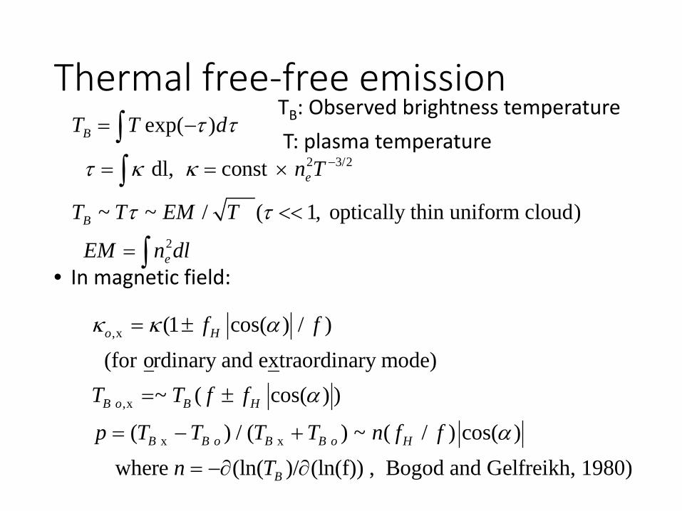
Thermal free-free emission TB: Observed brightness temperature T: plasma temperature
• In magnetic field:
2 3/2
2
exp( )
dl, const
~ ~ / ( 1, optically thin uniform cloud)
B
e
B
e
T T d
n T
T T EM T
EM n dl
τ τ
τ κ κ
τ τ
−
= −
= = ×
<<
=
∫∫
∫
,x
,x
x x
(1 cos( ) / ) (for ordinary and extraordinary mode)
~ ( cos( ) )
( ) / ( ) ~ ( / ) cos( ) where (ln( )/ (ln(f)) , Bogod and Gelfreikh, 1980)
o H
B o B H
B B o B B o H
B
f f
T T f f
p T T T T n f fn T
κ κ α
α
α
= ±
= ±
= − +
= −∂ ∂
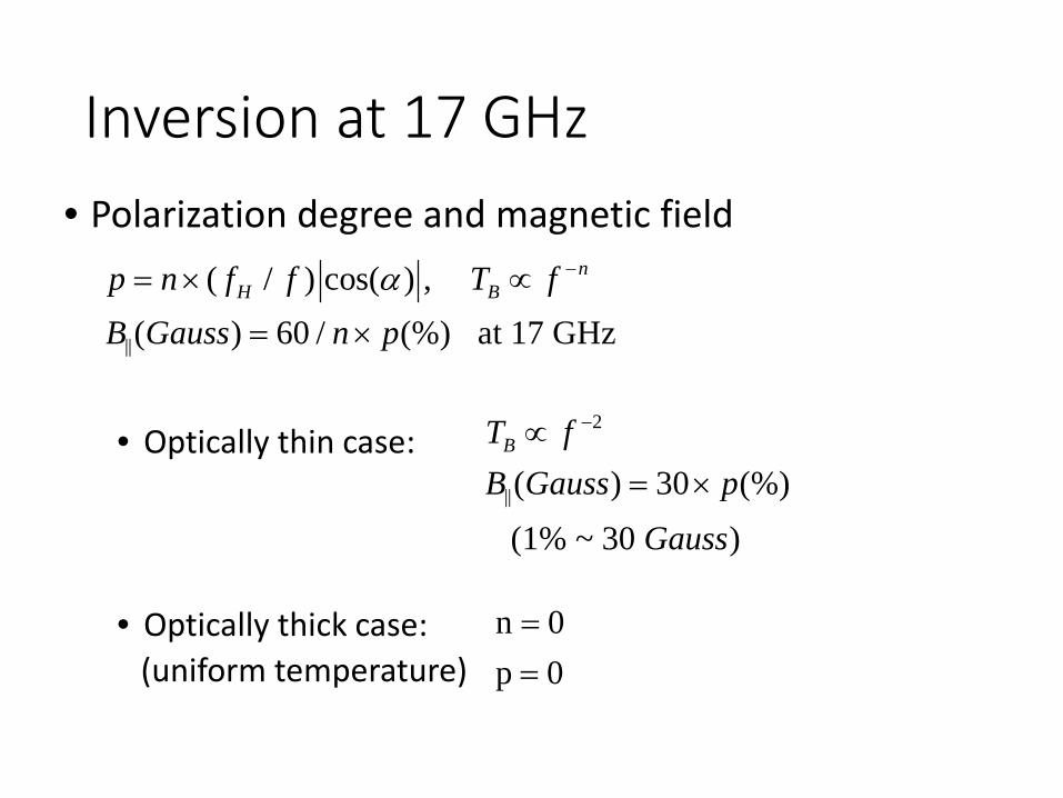
Inversion at 17 GHz • Polarization degree and magnetic field
• Optically thin case:
• Optically thick case: (uniform temperature)
||
( / ) cos( ) , ( ) 60 / (%) at 17 GHz
nH Bp n f f T f
B Gauss n pα −= × ∝
= ×
2
||
( ) 30 (%) (1% ~ 30 )
BT fB Gauss p
Gauss
−∝= ×
0p 0n
==
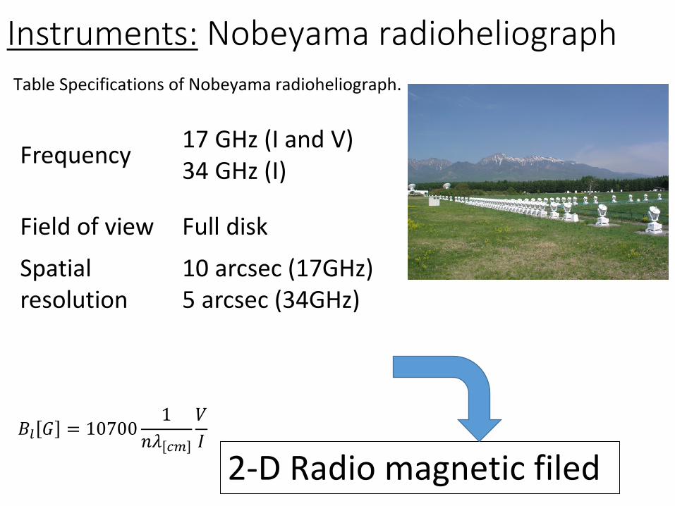
Instruments: Nobeyama radioheliograph
7
Frequency 17 GHz (I and V) 34 GHz (I)
Field of view Full disk
Spatial resolution
10 arcsec (17GHz) 5 arcsec (34GHz)
Table Specifications of Nobeyama radioheliograph.
2-D Radio magnetic filed
1 frequency band for polarization 2 frequency bands for intensity
𝐵𝐵𝑙𝑙 𝐺𝐺 = 107001
𝑛𝑛𝜆𝜆 𝑐𝑐𝑐𝑐
𝑉𝑉𝐼𝐼

4. Post flare arcade of loops
2014/12/04 IAUS305@Costa Rica 8
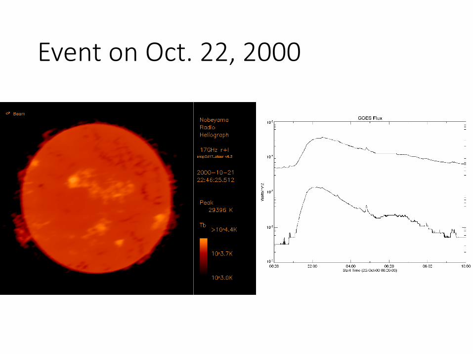
Event on Oct. 22, 2000
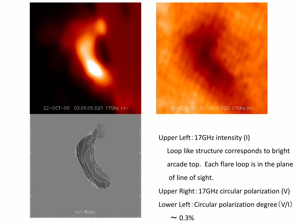
Upper Left:17GHz intensity (I)
Loop like structure corresponds to bright
arcade top. Each flare loop is in the plane
of line of sight.
Upper Right:17GHz circular polarization (V)
Lower Left:Circular polarization degree(V/I)
~ 0.3%

Mag. field distribution(~10 Gauss)

Post flare arcade of loops on Oct. 22, 2000
• optically thin thermal f-f (Tb ratio at 34 and 17 GHz is about 1/4)
• Uniform circular polarization along the arcade with 0.3 % (~10 G)
• magnetic field increases upwards (EM weighted mag. field strength)
• suggests loop structure, not cusp structure

Measured mag. field strength increases upwards
Measured mag. field strength decreases upwards due to Cusp shape

YOHKOH Observation Soft X-ray Telescope(SXT) Tsuneta (1997)
?
5. Magnetic field in the Chromosphere (optically thick case with temperature gradient)
2014/12/04 IAUS305@Costa Rica 15

Polarization at the chromosphere
16
𝑃𝑃 =𝑇𝑇𝐵𝐵,𝑥𝑥 − 𝑇𝑇𝐵𝐵,𝑜𝑜
𝑇𝑇𝐵𝐵,𝑋𝑋 + 𝑇𝑇𝐵𝐵,𝑜𝑜
Thermal bremsstrahlung (Free-free emission) at microwave range
At the chromosphere 𝜏𝜏 ≈ 1
Temperature gradient 𝑇𝑇𝐵𝐵,𝑜𝑜 ≠ 𝑇𝑇𝐵𝐵,𝑥𝑥 Polarization
Magnetic field 𝜏𝜏𝑜𝑜 ≠ 𝜏𝜏𝑥𝑥
penetrate into different layers
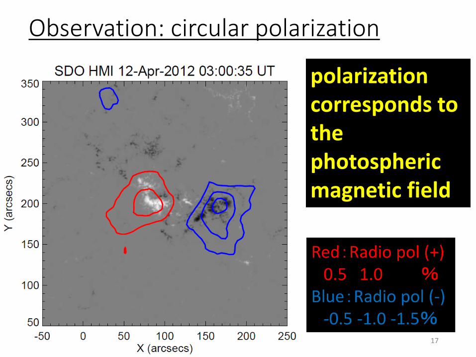
Observation: circular polarization
17
polarization corresponds to the photospheric magnetic field
Red:Radio pol (+) 0.5 1.0 % Blue:Radio pol (-) -0.5 -1.0 -1.5%

Radio Magnetic filed
18
𝐵𝐵𝑙𝑙 𝐺𝐺 = 107001
𝑛𝑛𝜆𝜆 𝑐𝑐𝑐𝑐
𝑉𝑉𝐼𝐼
HMI (G) Radio (G) Ratio FP+ 568 116 0.20 FP- -456 -217 0.47
circular polarization deg. Green: n, Red: Mag. Field (N), Blue: (S) +
Radio Magnetic filed is derived
n: = 𝜕𝜕log 𝑇𝑇𝐵𝐵𝜕𝜕log 𝜆𝜆
Green contours
6. Summary
• Simple examples of magnetic field measurements are presented using radio imaging instrument (NoRH)
• Coronal magnetic field in a post flare arcade of loops (optically thin, uniform temperature) • Chromospheric magnetic field in an active region (optically thick with temperature gradient)
• There are other ways of measuring magnetic field • Measurement of sunspot magnetic field using gyro-resonance
emission mechanism (highly polarized bright source above sunspots)
• Measurement of very weak magnetic field in the upper corona or in the inter-planetary space using Faraday rotation mechanism (linear polarization position angle rotate with frequency)
• Measurement of magnetic field filled with non-thermal electrons (accelerated in solar flares) due to gyro-synchrotron emission
• and others.
2014/12/04 IAUS305@Costa Rica 19

Abstract
2014/12/04 IAUS305@Costa Rica 21
Circularly polarized radio waves interact with gyrating electrons in the magnetic field due to the Lorentz force. Emissivity and absorption coefficients of right hand circular polarization (RCP) and that of left hand circular polarization (LCP) are different. This is the essence of magnetic field measurements with radio technique. Inversion procedure is rather simple because these processes can be treated by classical theory of electromagnetism and mechanics. In thermal plasma, emissivity and absorption coefficient of radio waves are strongly coupled and their ratio is approximated by Rayleigh-Jeans formula. Optical depths (line-of-sight integrated absorption coefficient) of RCP and LCP differ in the presence of magnetic field. The radio intensity difference between RCP and LCP (Stokes parameter V) can be used to measure line-of-sight magnetic field strength. Measurement of magnetic field strength in the corona is rather simple due to small optical depth. Even in optically thick chromosphere, we can estimate magnetic field strength due to steep temperature gradient. Examples of magnetic field distribution in the corona and in the chromosphere observed by the Nobeyama Radioheliograph will be presented. There are other methods to estimate magnetic field strength using radio techniques in the solar atmosphere and also in the interplanetary space. These methods will also be reviewed.
Recommended