University of Alberta
Protection and Power Quality Impact of Distributed Generation on
Distribution System
by
Hesam Yazdanpanahi
A thesis submitted to the Faculty of Graduate Studies and Research
in partial fulfillment of the requirements for the degree of
Doctor of Philosophy
in
Power Engineering and Power Electronics
Department of Electrical and Computer Engineering
©Hesam Yazdanpanahi
Spring 2014
Edmonton, Alberta
Permission is hereby granted to the University of Alberta Libraries to reproduce single copies of this
thesis and to lend or sell such copies for private, scholarly or scientific research purposes only. Where the
thesis is converted to, or otherwise made available in digital form, the University of Alberta will advise
potential users of the thesis of these terms.
The author reserves all other publication and other rights in association with the copyright in the thesis
and, except as herein before provided, neither the thesis nor any substantial portion thereof may be printed or
otherwise reproduced in any material form whatsoever without the author's prior written permission.

Abstract
Distributed Generation (DG) units are relatively small generation plants
directly connected to the distribution networks as alternatives for bulky power
plants and to integrate renewable energy sources into the power system. Despite
their several advantages, DGs have a serious impact on the distribution system. In
this thesis, the main focus is on the DGs’ impact on the Over-Current (O.C.)
protection system’s coordination and also on the power quality.
DGs are known to contribute fault currents to their interconnected power
system. As a result, DGs may affect the coordination of O.C. protection in a
distribution system. This problem is expected to become more acute as industry is
moving towards requiring DGs to stay connected during faults (i.e., requiring low
voltage ride through capability). This thesis presents its findings on the
contributions of DGs to fault currents and their probable impact on the O.C.
protection coordination. This thesis also presents techniques to mitigate the
impact of Inverter-Based DGs (IBDGs) and Synchronous Machine DGs
(SMDGs), as their impact on the O.C. protection, especially for marginal
coordination, is more significant than that of other types of DG.
In the discussion of the DG’s impact on the power quality, the main focus is
on the harmonic modelling and analysis of Doubly-Fed Induction Generator
(DFIG)-based wind farms. An accurate modeling method is proposed in this
thesis. Also, the harmonic emissions of these DGs are compared to the limits

determined by power quality standards. The findings show that the harmonic
emissions of DFIG-based wind farms are too low to concern utility operators.

Table of Contents
CHAPTER 1 INTRODUCTION ................................................................................................... 1
1.1 DISTRIBUTED GENERATION (DG) .............................................................................................1
1.2 DG TYPES .................................................................................................................................2
1.3 DGS’ IMPACT ON DISTRIBUTION SYSTEM ..................................................................................3
1.3.1 DGs’ impact on the O.C. protection system ...................................................................3
1.3.2 DGs’ impact on power quality .......................................................................................6
1.4 THESIS SCOPES AND OUTLINE ...................................................................................................6
1.5 RESEARCH CONTRIBUTION .......................................................................................................7
CHAPTER 2 IMPACT OF DG ON THE OVER-CURRENT (O.C.) PROTECTION .......... 10
2.1 MISCOORDINATION BETWEEN MAIN AND BACK-UP PROTECTION ............................................ 10
2.2 FAILURE IN FUSE SAVING SCHEME .......................................................................................... 12
2.3 FALSE TRIPPING ...................................................................................................................... 13
2.4 DESENSITIZATION (REDUCTION IN REACH) ............................................................................. 13
2.5 CONCLUSION .......................................................................................................................... 14
CHAPTER 3 IMPACT OF INVERTER-BASED DGS ON O.C. PROTECTION ................. 15
3.1 INVERTERS’ CONTROL STRATEGIES ........................................................................................ 15
3.1.1 Voltage-controlled voltage source inverters ................................................................ 15
3.1.2 Current-controlled voltage source inverters ................................................................ 16
3.2 INVERTERS’ O.C. PROTECTION ............................................................................................... 17
3.2.1 DG trip ......................................................................................................................... 17
3.2.2 Current limiting protection .......................................................................................... 18
3.3 CONTRIBUTION OF IBDGS TO FAULT CURRENT ...................................................................... 19
3.4 IMPACT OF DG ON FUSE-RECLOSER COORDINATION ............................................................... 21
3.5 THE PROPOSED STRATEGY ...................................................................................................... 26
3.6 SIMULATION RESULTS ............................................................................................................ 28
3.6.1 Performance during low impedance faults .................................................................. 28
3.6.2 Performance during high impedance faults ................................................................. 35
3.6.3 Performance during non-fault disturbances ................................................................ 36
3.7 CONCLUSION .......................................................................................................................... 39
CHAPTER 4 IMPACT OF SYNCHRONOUS-MACHINE DGS ON O.C.
PROTECTION ................................................................................................................................ 41
4.1 OPERATIONAL REACTANCES AND TIME CONSTANTS ............................................................... 43
4.2 SYNCHRONOUS GENERATOR’S FAULT CURRENT ..................................................................... 46
4.3 CASE STUDIES ........................................................................................................................ 49
4.3.1 Impact on the main and back-up protection coordination ........................................... 49
4.3.2 Impact on fuse-saving scheme ...................................................................................... 52
4.4 IDEA OF UTILIZING FIELD DISCHARGE CIRCUIT ....................................................................... 54
4.5 DETAILED ANALYSIS .............................................................................................................. 59
4.6 FIELD DISCHARGE CIRCUIT DESIGN PROCEDURE ..................................................................... 70
4.6.1 Field discharge resistance ........................................................................................... 71
4.6.2 Current and voltage ratings of solid state switches ..................................................... 73
4.6.3 Grid fault detection ...................................................................................................... 74
4.7 MITIGATION OF SMDG’S IMPACT ON COORDINATION: CASE STUDIES .................................... 75
4.7.1 Case I: Field discharge circuit design ......................................................................... 75
4.7.2 Case II: main and back-up relays coordination ........................................................... 77
4.7.3 Case III: Fuse-recloser coordination ........................................................................... 78
4.8 IMPACT OF FIELD DISCHARGE ON VOLTAGE RECOVERY .......................................................... 79
4.9 IMPACT OF FIELD DISCHARGE ON GENERATOR’S STABILITY ................................................... 85
4.10 CONCLUSION .......................................................................................................................... 89
CHAPTER 5 HARMONIC ANALYSIS OF DFIG-BASED WIND FARMS ......................... 91
5.1 METHODOLOGY ...................................................................................................................... 92
5.2 SINUSOIDAL PWM SWITCHING TECHNIQUE ............................................................................ 96
5.3 HARMONIC MODELLING OF DFIG SYSTEM ............................................................................. 99
5.3.1 Harmonic modelling of GSC ...................................................................................... 100
5.3.2 Harmonic modelling of RSC ...................................................................................... 101
5.4 SIMULATION ......................................................................................................................... 102
5.4.1 Simulated system ........................................................................................................ 102
5.4.2 Simulation results ....................................................................................................... 104
5.4.3 Comparison of the results .......................................................................................... 109
5.5 ESTIMATION OF PARAMETERS .............................................................................................. 111
5.5.1 Stator and rotor powers ............................................................................................. 111
5.5.2 Estimation of Vdc and MGSC ........................................................................................ 113
5.5.3 Estimation of MRSC ..................................................................................................... 114
5.6 ILLUSTRATIVE EXAMPLE ...................................................................................................... 115
5.6.1 Study scenario ............................................................................................................ 115
5.6.2 Example...................................................................................................................... 116
5.7 NON-CHARACTERISTIC HARMONICS ..................................................................................... 118
5.8 COMPARISON WITH OTHER HARMONIC SOURCES AND STANDARDS ...................................... 120
5.9 CONCLUSION ........................................................................................................................ 123

CHAPTER 6 CONCLUSIONS AND FUTURE WORK ......................................................... 125
6.1 THESIS CONCLUSIONS AND CONTRIBUTIONS ......................................................................... 125
6.2 SUGGESTIONS FOR FUTURE WORK ........................................................................................ 127
CHAPTER 7 REFERENCES .................................................................................................... 129
APPENDIX A: FAULT CURRENT CONTRIBUTION OF INDUCTION-MACHINE
DGS ............................................................................................................................... 138
A.1 INDUCTION GENERATOR’S FAULT CURRENT ......................................................................... 138
A.1.1 Singly-Fed Induction Generator (SFIG) .................................................................... 139
A.1.2 Doubly-Fed Induction Generator (DFIG) ................................................................. 144
A.2 FINDINGS FROM AN EXPERIMENTAL RESEARCH WORK.......................................................... 146
A.3 IMPACT ON THE PROTECTION COORDINATION ....................................................................... 147
A.3.1 PHASE-TO-PHASE FAULTS ..................................................................................................... 148
A.3.2 PHASE-TO-GROUND FAULTS ................................................................................................. 149
A.4 CONCLUSION ........................................................................................................................ 150
APPENDIX B: FAULT CURRENT CONTRIBUTION OF PERMANENT MAGNET
SYNCHRONOUS GENERATORS .................................................................................................. 152
B.1 PMSG’S FAULT CURRENT .................................................................................................... 153
B.2 COMPARISON OF PMSG’S AND WFSG’S FAULT CURRENTS ................................................. 154
B.3 ESTIMATION OF PMSG’S CONTRIBUTION TO FAULT ............................................................. 157
B.4 LIMITING PMSG’S FAULT CURRENT ..................................................................................... 158
B.4.1 PM machines with large leakage inductance ............................................................. 159
B.4.2 PM machines with auxiliary excitation ...................................................................... 160
B.4.3 PM machines with mechanically adjustable flux ....................................................... 163
B.5 CONCLUSION ........................................................................................................................ 165
REFERENCES OF APPENDICES ............................................................................................................. 167

List of Tables
Table 3-1: IEEE std. 1547 required response to abnormal voltage conditions ..... 27
Table 3-2: Test system parameters ....................................................................... 37
Table 3-3: Induction machine’s parameters .......................................................... 37
Table 4-1: Comparison of impedance estimation method with data-based single-
point problem [61] ................................................................................................ 46
Table 4-2: Loads and their power factors ............................................................. 50
Table 4-3: Relays’ settings .................................................................................... 51
Table 4-4: Fault currents and relays’ operation times........................................... 51
Table 4-5: Operational constants of simulated synchronous machine [62] .......... 51
Table 4-6: Sections’ lengths .................................................................................. 53
Table 4-7: Loads and their power factors ............................................................. 53
Table 4-8: Field discharge switches’ ratings......................................................... 74
Table 4-9: Switches’ ratings in the studied case ................................................... 76
Table 4-10: The relays’ currents and operation times for fault at F3 and 6.5MW
DG ......................................................................................................................... 78
Table 4-11: CCT for 3-phase solid fault at different busses ................................. 89
Table 5-1: Sample spectrum for background harmonic voltages in Scenario 1 ... 94
Table 5-2: Vh/Vdc in PWM technique with large odd mf multiple of 3 ................ 99
Table 5-3: Vh in PWM technique with mf =45, fsw=2.7kHz, M=.8 and Vdc=1150V
............................................................................................................................. 101
Table 5-4: Major harmonic components of GSC current ................................... 107
Table 5-5: Major harmonic components of RSC current .................................... 107
Table 5-6: Harmonic components at 2580 Hz .................................................... 110
Table 5-7: Harmonic components at 3300 Hz .................................................... 111
Table 5-8: Major harmonic components the example in the worst condition .... 118
Table 5-9: Normalized spectrum of harmonic sources ....................................... 121
Table 5-10: Comparison of the farm’s harmonic currents with the limits of IEEE
Std. 1547 ............................................................................................................. 122

Table 5-11: Comparison of the farm’s harmonic voltages with the limits of IEC
61000-3 ............................................................................................................... 122
List of Figures
Figure 1-1: Comparison of power networks: (a) Traditional network, (b) Network
with DG ................................................................................................................... 2
Figure 1-2: Proposed WECC LVRT standard [14] ................................................. 5
Figure 2-1: Sample distribution feeder with main and back-up protection .......... 11
Figure 2-2: Time-current characteristic curves of main and back-up devices of
Figure 2-1 .............................................................................................................. 11
Figure 2-3: Typical response time of O.C. devices versus fault current [21] ....... 12
Figure 2-4: Impact of the DG on the fuse-recloser coordination .......................... 13
Figure 2-5: False tripping due to DG’s response to fault at adjacent feeder [23] . 13
Figure 2-6: Desensitization or reduction in reach. ................................................ 14
Figure 3-1: Voltage-controlled voltage source inverter with its control blocks ... 16
Figure 3-2: Equivalent circuit of voltage-controlled voltage source inverter [27] 16
Figure 3-3: Current-controlled voltage source inverter with its control blocks .... 17
Figure 3-4: Equivalent circuit of current-controlled voltage source inverter [27] 17
Figure 3-5: Typical inverter’s RMS current during the fault (trip protection) ..... 18
Figure 3-6: Typical inverter’s RMS current during the fault (current limiting
protection) ............................................................................................................. 18
Figure 3-7: Response of a commercial inverter with current limiting protection to
3-phase fault [33] .................................................................................................. 20
Figure 3-8: Response of another commercial inverter with current limiting
protection to 3-phase fault [[33]............................................................................ 20
Figure 3-9: Response of inverter with current limiting protection proposed in [31]
to 3-phase fault ...................................................................................................... 21
Figure 3-10: Fuse-Recloser protection scheme in distribution feeders ................ 22
Figure 3-11: Fuse-Recloser time-current characteristic curves ............................ 22
Figure 3-12: Impact of DG on operation of protection system under low
impedance fault situation ...................................................................................... 22
Figure 3-13: Equivalent circuit of a distribution system with inverter-based DG,
during a downstream fault. ................................................................................... 23

Figure 3-14: Voltage and current vector diagram of: a) DG provides active power,
b) DG provides reactive power. ............................................................................ 26
Figure 3-15: Proposed strategy to determine inverter reference current .............. 28
Figure 3-16: IEEE 13-Node test feeder system [40] ............................................. 29
Figure 3-17: Fuse-recloser coordination in the simulated system ........................ 29
Figure 3-18: Difference between fuse and recloser operation time after adding DG
for 0.01 Ohm fault ................................................................................................. 30
Figure 3-19: Difference between fuse and recloser operation time after adding DG
for 0.1 Ohm fault ................................................................................................... 30
Figure 3-20: Intentional phase shift in DG current during voltage sag to support
voltage. .................................................................................................................. 32
Figure 3-21: Difference between fuse and recloser operation time for 0.01 Ohm
fault with pi/2 phase shift in inverter current. ....................................................... 32
Figure 3-22: Difference between fuse and recloser operation time for 0.1 Ohm
fault with pi/2 phase shift in inverter current. ....................................................... 32
Figure 3-23: Difference between fuse and recloser operation time for 0.2 Ohm
fault with pi/2 phase shift in inverter current. ....................................................... 32
Figure 3-24: Difference between fuse and recloser operation time for 0.01 Ohm
fault with inverter current reduction control. ........................................................ 33
Figure 3-25: PCC voltage for 0.01 Ohm fault with DG at 30% penetration level.33
Figure 3-26: DG output current for 0.01 Ohm fault with DG at 30% penetration
level. ...................................................................................................................... 33
Figure 3-27: Fuse current for 0.01 Ohm fault with DG at 30% penetration level. 33
Figure 3-28: Output current of inverter installed at Node 634. ............................ 34
Figure 3-29: Output current of inverter installed at Node 634. ............................ 34
Figure 3-30: Fuse current for.1 Ohm fault with DG units at Nodes 634 and 675. 34
Figure 3-31: Output current of inverters for 2-Ohm fault in the middle of 645-646.
............................................................................................................................... 35
Figure 3-32: Inverter output power for 8-Ohm fault in the middle of 645-646. ... 35
Figure 3-33: PCC voltage for 8-Ohm fault in the middle of 645-646. ................. 36
Figure 3-34: Fuse current for 8-Ohm fault in the middle of 645-646. .................. 36

Figure 3-35: A distribution network with fuse-saving protection. ....................... 37
Figure 3-36: A distribution network with fuse-saving protection. ....................... 38
Figure 3-37: DG output power during motor starting for both traditional and
proposed control strategies.................................................................................... 38
Figure 3-38: Voltage at terminals of IM during motor starting for both traditional
and proposed control strategies. ............................................................................ 38
Figure 3-39: Inverter output current during the motor starting transient. ............. 39
Figure 4-1: SMDG control strategies during grid fault ........................................ 43
Figure 4-2: Synchronous generator’s structure ..................................................... 44
Figure 4-3: Equivalent synchronous machine with fictitious d- and q-axis
windings ................................................................................................................ 44
Figure 4-4: Typical synchronous generator’s fault current: (a) Complete
waveform, (b) first 18 cycles ................................................................................ 49
Figure 4-5: Single-line diagram of the studied case ............................................. 50
Figure 4-6: Fault current at F3 when a 5MW SMDG is added at substation ....... 52
Figure 4-7: Impact of 6.5MW SMDG on relays’ operation points ....................... 52
Figure 4-8: Single-line diagram of sample network ............................................. 52
Figure 4-9: fuse and recloser time-current characteristics curves ......................... 54
Figure 4-10: Fuse and recloser fault current when a 1600kW SMDG is added at
bus 1 ...................................................................................................................... 54
Figure 4-11: Impact of a 2400kW SMDG on coordination .................................. 54
Figure 4-12: A synchronous generator with its field discharge circuit ................. 56
Figure 4-13: A sample distribution network with synchronous-machine DG ...... 57
Figure 4-14: RMS of machine’s output current during 3-phase fault at point F .. 57
Figure 4-15: RMS of ac component of machine’s output current during 3-phase
fault at point F ....................................................................................................... 58
Figure 4-16: RMS of machine’s output current during 1-phase fault at point F .. 58
Figure 4-17: RMS of ac component of machine’s output current during 1-phase
fault at point F ....................................................................................................... 59
Figure 4-18: Voltage which appears at the field winding during the fault ........... 59

Figure 4-19: Synchronous generator’s fault current with short circuited field
winding, (a) Complete waveform, (b) first 18 cycles ........................................... 62
Figure 4-20: Synchronous generator’s fault current with discharge resistance in
series with field winding, (a) Complete waveform, (b) first 6 cycles ................... 63
Figure 4-21: Accurate estimation of the synchronous generator’s fault current
with a discharge resistance in series with its field ................................................ 64
Figure 4-22: Synchronous generator’s fault current with field discharge operation,
(a) Complete waveform, (b) first 9 cycles ............................................................ 66
Figure 4-23: A sample distribution feeder with SMDG ....................................... 67
Figure 4-24: RMS ac component of generator’s fault current with field discharge
operation in the system shown in Figure 4-21 ...................................................... 67
Figure 4-25: Reduction in synchronous generator’s RMS ac component of fault
current due to applying field discharge ................................................................. 68
Figure 4-26: Reduction in generator’s RMS ac component of fault current for
different values of field discharge resistance ........................................................ 69
Figure 4-27: Fault current components of synchronous generator, (a) When
traditional excitation is applied, (b) when field discharge is applied.................... 70
Figure 4-28: Synchronous generator’s field current during the three-phase fault at
its terminals, with field discharge circuit operation .............................................. 72
Figure 4-29: Rotor’s circuit during field discharge circuit operation ................... 73
Figure 4-30: Field’s current derivative for three different grid disturbances ....... 75
Figure 4-31: Field winding’s maximum voltage due to discharge circuit operation
............................................................................................................................... 76
Figure 4-32: Effect of field discharge circuit on eliminating the impact of a
6.5MW SMDG ...................................................................................................... 78
Figure 4-33: Fuse and recloser fault current when a 1600kW DG is added at bus 1
............................................................................................................................... 79
Figure 4-34: Effect of field discharge circuit to eliminate the impact of a 2400kW
DG on coordination ............................................................................................... 79
Figure 4-35: Impact of field discharge on reactive power consumption during and
after fault ............................................................................................................... 80

Figure 4-36: Impact of field discharge on voltage recovery ................................. 80
Figure 4-37: A distribution feeder with DG located close to the source .............. 81
Figure 4-38: A distribution feeder with DG located far from the source ............. 81
Figure 4-39: Reactive power recovery .................................................................. 81
Figure 4-40: Terminal voltage recovery ............................................................... 82
Figure 4-41: d-axis flux ........................................................................................ 82
Figure 4-42: d-axis flux ........................................................................................ 82
Figure 4-43: SMDG with modified field discharge circuit ................................... 83
Figure 4-44: Reactive power recovery .................................................................. 84
Figure 4-45: Terminal voltage recovery ............................................................... 84
Figure 4-46: d-axis flux ........................................................................................ 84
Figure 4-47: Output current .................................................................................. 85
Figure 4-48: Exciter voltage ................................................................................. 85
Figure 4-49: Sample distribution network simulated for stability studies ............ 86
Figure 4-50: Generator’s output current and rotor angle deviation for .1 sec. 3-
phase fault at terminals ......................................................................................... 87
Figure 4-51: Generator’s d-axis flux during and after fault .................................. 87
Figure 4-52: Generator’s output power and rotor angle deviation for .2 sec. 3-
phase fault 8.1 km away from generator ............................................................... 88
Figure 5-1: DFIG-based wind farm structure ....................................................... 92
Figure 5-2: DFIG’s equivalent circuit at fundamental frequency ......................... 92
Figure 5-3: DFIG’s equivalent circuit for harmonic analysis ............................... 93
Figure 5-4: DC link voltage .................................................................................. 95
Figure 5-5: Zoomed DC link voltage .................................................................... 95
Figure 5-6: Spectrum of DC link voltage ............................................................. 95
Figure 5-7: Spectrum of DC link voltage in lower frequencies ............................ 95
Figure 5-8: Integer harmonics of GSC’s terminal voltage .................................... 96
Figure 5-9: Three-phase voltage source converter’s structure .............................. 97
Figure 5-10: Carrier and reference signals in 3-phase sinusoidal PWM scheme . 97
Figure 5-11: Switching states of S1 during a period ............................................. 97
Figure 5-12: Line-line voltages at converter’s terminals ...................................... 97

Figure 5-13: Harmonic spectrum of a 3-phase sinusoidal PWM switching [76] . 99
Figure 5-14: Harmonic modelling of GSC at its hth harmonic............................ 100
Figure 5-15: DFIG’s equivalent circuit at hth harmonic frequency ..................... 102
Figure 5-16: Harmonic modelling of RSC at its hth harmonic ............................ 102
Figure 5-17: Simulated power system ................................................................ 103
Figure 5-18: Details of wind farm simulation ..................................................... 103
Figure 5-19: DC link voltage .............................................................................. 105
Figure 5-20: Harmonic spectrum of GSC’s current (% of converter’s fundamental
current) ................................................................................................................ 105
Figure 5-21: Harmonic spectrum of GSC’s current (% of generator’s fundamental
current) ................................................................................................................ 106
Figure 5-22: Harmonic spectrum of RSC’s current (% of converters fundamental
current, fundamental frequency=12 Hz) ............................................................. 106
Figure 5-23: Harmonic spectrum of RSC’s current (% of generator’s fundamental
current) ................................................................................................................ 106
Figure 5-24: Harmonic spectrum of stator’s current ........................................... 108
Figure 5-25: Harmonic spectrum of I4 ................................................................ 108
Figure 5-26: Harmonic spectrum of I5 ................................................................ 109
Figure 5-27: Harmonic spectrum of voltage ....................................................... 109
Figure 5-28: Equivalent DFIG model ................................................................. 110
Figure 5-29: A typical cp over λ curve ................................................................ 112
Figure 5-30: Power sharing in a loss-less DFIG system ..................................... 112
Figure 5-31: Equivalent circuit of GSC at fundamental frequency during steady
state ..................................................................................................................... 113
Figure 5-32: Normalized amplitude of mf-1-th harmonic for different values of M
............................................................................................................................. 115
Figure 5-33: Equivalent circuit for calculation of harmonic currents caused by
GSC ..................................................................................................................... 118
Figure 5-34: Equivalent circuit for calculation of harmonic currents caused by
RSC ..................................................................................................................... 118

Figure 5-35: Normalized harmonic components of voltage at GSC terminals, (a)
up to 48th
harmonic, (b) up to 21st harmonic ....................................................... 119
Figure 5-36: PWM reference signal of GSC ....................................................... 120
Figure 5-37: Normalized spectrum of PWM reference signal of GSC ............... 120
List of acronyms
DG Distributed Generation
IBDG Inverter-based Distributed Generation
IMDG Induction-Machine Distributed Generation
SMDG Synchronous-Machine Distributed Generation
O.C. Over-Current
IG Induction Generator
SCIG Squirrel-Cage Induction Generator
DFIG Doubly-Fed Induction Generator
LG Line-to-Ground
SG Synchronous Generator
PMSG Permanent Magnet Synchronous Generator

List of symbols
Instantaneous voltage of stator
RMS voltage of stator
Instantaneous voltage of rotor
Instantaneous current of stator
Instantaneous current of rotor
Instantaneous flux of stator
Instantaneous flux of rotor
Synchronous angular speed
Rotor’s angular speed
Induction machine’s Stator’s resistance
Rotor’s resistance
Stator’s total inductance
Rotor’s total inductance
Stator-rotor mutual inductance
Stator’s leakage inductance
Rotor’s leakage inductance
Stator’s transient inductance
Rotor’s transient inductance
Stator’s transient time constant
Rotor’s transient time constant
Stator’s coupling factor
Rotor’s coupling factor
Stator voltage phase angle at fault instance
Leakage factor
External resistance
Total flux linkage of d-axis
Total flux linkage of q-axis
Laplace operator
Angular velocity

Field winding resistance
Synchronous machine’s Stator resistance
d-axis damper winding resistance
q-axis damper winding resistance
Field excitation voltage
Instantaneous d-axis machine’s terminal voltage
Instantaneous q-axis machine’s terminal voltage
d-axis machine’s terminal voltage magnitude
q-axis machine’s terminal voltage magnitude
d-axis winding’s current
q-axis winding’s current
Field winding’s current
Ac component of generator’s current at phase a
RMS of ac component of generator’s current at phase a
Reduction in RMS of ac component of generator’s fault current due to field
discharge
d-axis winding’s total inductance
d-axis winding’s mutual inductance
Laplace transform of d-axis winding’s reactance
Laplace transform of q-axis winding’s reactance
d-axis synchronous reactance
q-axis synchronous reactance
d-axis winding’s mutual reactance
q-axis winding’s mutual reactance
d-axis damper winding’s leakage reactance
q-axis damper winding’s leakage reactance
Armature leakage reactance
d-axis transient short-circuit time constant
d-axis sub-transient short-circuit time constant
d-axis transient open-circuit time constant
d-axis sub-transient open-circuit time constant

q-axis sub-transient short-circuit time constant
q-axis sub-transient open-circuit time constant
Armature time constant

Chapter 1: Introduction
1
Chapter 1
Introduction
This chapter presents the concepts and definitions that will be frequently referred
to in the rest of this thesis, the thesis objectives and outline, and the research
contributions.
1.1 Distributed Generation (DG)
For decades, the only way to supply customers was to transmit electrical
energy from bulky centralized generation plants to the distribution side via
transmission lines, and then to deliver this energy to customers through
distribution system. Later, Distributed Generation (DG) was introduced into
utilities. DG units are relatively small generation plants with capacities lower than
30MW and are directly connected to the distribution networks. Figure 1-1
compares a traditional network with a network in which a DG is embedded. In
this figure, the arrows represent the direction of the power felow.
Some of the most important advantages that DG units provide for utilities are
as follows:
1. A DG is an alternative for satisfying incremental demand without any
need for transmission expansion [1].
2. Since the DG is directly connected to the distribution network, the
DG’s current does not flow through the transmission line. Therefore,
the associated losses are decreased.
3. The DG concept enable renewable energy sources such as PV, wind,
and fuel cells to be integrated into the power system [2]. Such
integration is a solution for universal concerns about the environment
and air pollution and is an alternative for the use of limited risky fossil
fuel resources.

Chapter 1: Introduction
2
4. DG units are capable of providing ancillary services to utilities,
including voltage regulation, reactive power compensation and active
filtering [3].
Generation
Transmission
Distribution
Consumer
(a)
Generation
Transmission
Distribution
Consumer
DG
(b)
Figure 1-1: Comparison of power networks: (a) Traditional network, (b) Network with DG
1.2 DG types
DG units are usually categorized based on their prime movers such as
Photovoltaic (PV) systems, diesel-generators, wind energy power plants, and
hydro power plants. However, this categorization is not useful for this study
because of the fact that the impact of DG units on the distribution system depend
mainly on their size and the electrical interfaces integrating them into the network.
In this thesis, DGs are categorized into four different types:
1. Inverter-based DGs (IBDGs): These DGs deliver power to the
network through a power electronic inverter and can be PV systems,
microturbines, fuel cells, or full-scale converter-based wind systems.

Chapter 1: Introduction
3
2. Synchronous-Machine DGs (SMDGs): These DGs deliver power to
the network through a synchronous generator, and the prime mover
can be a diesel engine, gas turbine, hydro turbine or wind turbine.
3. Induction-Machine DGs: These DGs deliver power to the network via
an induction generator, and the prime mover can be either a wind or a
small hydro turbine.
4. Permanent Magnet Synchronous Generator (PMSG) DGs: In these
DGs, the power is transferred to the electrical system via a PMSG.
This technology has been used in some small hydro power plants.
1.3 DGs’ impact on distribution systems
Despite their undoubted advantages, DG systems have a negative impact on
the distribution system. Each utility follows a specific guideline or standard for
interconnecting DGs with the grid. Usually, these standards or guidelines include
the technical specifications and requirements which a DG must satisfy. Therefore,
these requirements should be considered in the study of the impact of DGs on
distribution systems. In this thesis, the main focus is on the DGs’ impact on the
Over-Current (O.C.) protection system’s coordination when Low Voltage Ride
Through (LVRT) is required by the utility, and also on the DG’s impact on the
power quality.
1.3.1 Low Voltage Ride Through
The impact on O.C. protection is one of the most important effects of DGs on
the distribution system. Before investigating this impact, one must understand the
two different approaches for the DG’s operation during the gird faults. In the first
approach, the DG interconnection guideline or standard requires the DG to cease
operation (to disconnect from the grid) when a fault happens. For example, IEEE
Std. 1547 [4] requires DG disconnection within .16 Sec. for Point of Common
Coupling (PCC) voltages lower than .5 per unit. Similarly, in some utility
companies in Canada such as ATCO Electric [5], Manitoba Hydro [6] and
ENMAX Power [7], an instantaneous DG trip is required for PCC voltages lower

Chapter 1: Introduction
4
than .5 per unit. In this approach, since the DG is disconnected from the grid, the
DG has no contribution to the fault current and, consequently, has no impact on
the O.C. protection. In fact, this approach has been practiced by many utilities
ever since the DG concept was first introduced, to prevent the DG from affecting
the protection.
However, after DGs penetrate significantly into some distribution systems,
the use of the DG disconnection approach can lead to the disconnection of a major
portion of the power generation and, consequently, can jeopardize the grid’s
stability. As a result, in such systems, grid codes are being modified [8], and in
some high and extra-high voltage grid connection standards like [9],[10] the
second approach is followed. In this approach, the distributed resources are forced
to stay connected to the grid during the fault. This approach has been extended to
some medium-voltage (1 kV<Vrated<60 kV) grids as well [11], [12] and is
expected to be the main approach in other guidelines such as IEEE Std. 1547 in
the near future [13]; i.e., the DG is required to stay connected during the
temporary fault to help maintain grid’s stability [14]. This requirement is named
Low Voltage Ride Through (LVRT). Figure 1-2 [14] demonstrates the proposed
2009 Western Electricity Coordination Council (WECC) LVRT standard. As this
figure reveals, in this standard, for 0% PCC voltage up to .15 Sec., the DG must
stay connected to the grid. Although DGs with LVRT capability support the grid’s
stability, they contribute to the fault current and, consequently, impact on the O.C.
protection. This impact, which will be covered in Chapter 2, can cause excessive
load loss and decrease service reliability. In fact, the main objective of DG’s
LVRT requirement is to avoid or minimize load loss by forcing the DG to
function similarly to traditional generation units by supporting grid’s stability and
post-fault voltage recovery. However, the conflict between LVRT and O.C.
protection can eventually cause an unnecessary load loss and a decrease in
reliability, two outcomes that contradict the LVRT’s fundamental objective. The
final goal of this thesis is to propose DG-side solutions to mitigate the conflict
between DG’s LVRT capability and O.C. protection coordination. Mitigating this

Chapter 1: Introduction
5
conflict will facilitate an increase in DG’s penetration and its associated
advantages without degrading the service reliability.
Figure 1-2: Proposed WECC LVRT standard [14]
1.3.2 DGs’ impact on the O.C. protection system
A distribution network and its protection system are designed based on the
assumptions that no generation unit is present in the network and that the network
is radial. These assumptions mean that no current source is present in the
distribution network; the short circuit level from the substation to the end of
feeders has a descending trend; and, for a certain fault at certain location the
current flows through the conductors from the substation to the fault location are
the same. In addition, these assumptions also mean that the current flow is
unidirectional from upstream (from the substation) to downstream. However,
adding a DG to a system may violate one or more of these assumptions and,
consequently, may cause serious problems in the protection system. Indeed, DGs
contribute fault currents to the distribution and, consequently, may affect the
coordination of O.C. protection in a distribution system. This issue becomes more
critical since utilities are moving towards requiring DGs to stay connected during
faults (i.e. low voltage ride through requirement).
Chapter 1: Introduction
6
1.3.3 DGs’ impact on power quality
DGs can cause different problems related to power quality, such as voltage
flicker, voltage dip and introducing harmonics into the network [15]-[17]. In this
thesis, we are interested in the harmonic modelling and analysis of DGs. The
harmonic emissions of SMDGs, IMDG and PMSGs are negligible. In contrast,
IBDGs are known as potential harmonic sources in the system. Several studies
have covered this subject for full-scale inverter-interfaced DGs [18]-[20].
However, Doubly-Fed Induction Generator (DFIG) based wind farms have not
been covered thoroughly. In these systems, a portion of the power is delivered
through the DFIG’s stator, and the rest is delivered through the inverters
connected to the rotor. In this type of DG, in contrast to the other types, two
harmonic sources exist. The first one, the converter at the grid side, directly
injects harmonic currents into the network, and the second one, the converter
connected to the DFIG’s rotor, induces harmonic currents in the stator side.
Moreover, these two converters share a DC link which makes the analysis more
complex. Furthermore, the DFIG is currently the most often used technology in
wind power generation. Consequently, the main focus is on the harmonic
modelling and analysis of this type of DG.
1.4 Thesis objectives and outline
One objective of this thesis is to determine the impact of different types of
DGs on O.C. protection and to propose new strategies to mitigate this negative
impact. This objective will be achieved in two stages:
Investigating the contribution of each type of DG to the fault current and
determining if each type can potentially impact the protection
coordination.
Proposing strategies to restrict the DGs’ contribution to fault current and,
consequently, to mitigate the DG’s impact on the protection system’s
coordination when LVRT is a requirement.
Another objective of this thesis is to analyze and model the harmonic
emission of DFIG-based wind farms.

Chapter 1: Introduction
7
The thesis is organized as follows:
Chapter 2 covers the impact of DG on O.C. protection. Chapter 3 presents our
investigation on the contribution of IBDGs to the fault current and proposes a
control strategy to restrict the contribution so that the DG does not impact the
coordination. The contribution of SMDGs to fault current is presented in Chapter
4, and a strategy is proposed to mitigate the impact of this type of DG on the
protection system by limiting the DG’s contribution. Harmonic analysis and
modelling of DFIG-based wind farms are presented in Chapter 5, which is
followed by conclusion in Chapter 6. Finally, Appendices A and B cover the
contribution of IMDGs and PMSGs, respectively, to fault current.
1.5 Research contribution
The key research contributions of this thesis can be summarized as follows:
A thorough investigation is conducted on inverter-based DGs’ impact on
O.C. protection coordination. It is shown that at high penetration levels or
in the case of tight coordination, these DGs can cause miscoordination
between the O.C. protection devices. To mitigate this problem, a strategy
is proposed and applied to the simulated DG. In this strategy, the
inverter’s current is restricted to a dynamically adjusted limit. In contrast
to the common practices in which a fixed pre-determined current limit is
used, this limit is determined based on the severity of the abnormality.
Through several case studies, it is shown that this strategy not only
mitigates the impact of a inverter-based DG on O.C. protection but also
facilitates the DG’s ride through short-term disturbances.
The contribution of synchronous-machine DGs to the fault current is
assessed from O.C. protection coordination perspective, and it is shown
that among the major DG types, these DGs make the highest contribution
to the fault, which lasts long enough to cause miscoordination between
O.C. protection devices. To minimize the contribution of these DGs to the
fault and, consequently, to mitigate or minimize their impact on O.C.
protection coordination, the idea of utilizing the field discharge circuit is

Chapter 1: Introduction
8
proposed in this thesis. Although field discharge has been utilized for
decades, it has been used mainly to protect the synchronous generator and
to accelerate the generation unit shut down. However, in this thesis, a new
application is proposed for this circuit and is used to mitigate the impact of
the DG on the grid. The simulation results show that a well-designed field
discharge circuit can significantly increase the maximum allowable DG
capacity by reducing its impact on O.C. protection coordination. In
addition, a design procedure is proposed for solid-state switch-based field
discharge circuits. The field discharge circuit’s design procedure has been
previously studied in some references. However, in previous studies, this
was based on field discharge circuits with DC field breakers. Since the
operation of such breakers can take up to .1 sec., they are not fast enough
to be useful for the proposed application. As a result, in this thesis a design
procedure is proposed for the solid-state switched-based discharge circuits.
Since these circuits operate almost instantly and in contrast to the DC field
breakers, the arcing phenomenon is not involved in these circuits, so the
design procedure differs from those in the published studies.
For induction-machine DGs, the contribution of different types of
induction generators to the fault current is investigated through both
mathematical analysis and simulation from the O.C. coordination
perspective. The assessments show that the fault current contribution time
of these DGs is too short to impact the coordination, so mitigation is
unnecessary. As a result, this part of the research is included as an
appendix.
For PMSM DGs, which can be connected directly to the distribution
system for some small hydro power plants, their contribution to the fault is
assessed through both analysis and simulation. These machines are
compared with the traditional wound-field synchronous generators, and it
is shown that the fault response of these machines has no transient part. As
a result, a machine reaches its steady state fault current only a few cycles

Chapter 1: Introduction
9
after the fault, and the machine’s contribution to the fault current is
significantly smaller than the contribution wound-field synchronous
machine of the same size. In summary, in this thesis, it is shown that a
well-designed PMSM is unlikely to impact on the O.C. protection
coordination, and as a result, this part of the research is included as an
appendix.
Regarding the harmonic emission of DFIG-based wind farms, a method is
proposed to calculate the harmonic current spectrum of a wind farm. In the
proposed method, power electronic converters are replaced with the
harmonic voltage sources. As a result, the equivalent circuit contains only
impedances and voltage sources, so that the harmonic assessment is very
easy. In this part of the thesis, in order to verify the accuracy of the
proposed modeling method, a wind farm is simulated and the harmonic
analysis results obtained from the simulation are compared with the results
obtained from the proposed model. The comparison shows that the model
is accurate, and that the assumptions on which the model’s development is
based are valid. In addition, the harmonic emission of the simulated wind
farm is compared with the harmonic emission of more well-known
harmonic sources as well as the harmonic limits determined by major
power quality standards. The comparison shows that DFIG-based wind
farms are not major harmonic sources and that these farms comply with
the power quality standards.

Chapter 2: Impact of DG on the Over-Current (O.C.) protection
10
Chapter 2
Impact of DG on the Over-Current
(O.C.) protection
When a fault happens in the distribution system, the adjacent DGs respond to
the fault. Depending on the size, type and the distance from the fault location,
each DG contributes a certain amount of current in a certain window of time, and
then, the DG’s current decreases to zero or to a negligible level. Both the
contribution level and the contribution time window should be considered during
protection studies. This section presents the probable impact of DGs on the O.C.
protection system and illustrates how the DGs’ contribution levels and
contribution time windows play a role in such an impact.
2.1 Miscoordination between main and back-up protection
The DG’s contribution to the fault current may increase the fault current,
which flows through the protection devices and makes them operate faster than
what was expected during the protection design. This phenomenon can cause a
loss of coordination between the main and back-up protection devices; i.e. the
back-up device may operate sooner than the main one. Such a miscoordination
results in the undesirable de-energization of the loads located between the back-up
and main protection.
Figure 2-1 shows a simple feeder with its protection devices. Figure 2-2
shows the time-current characteristic curves of these devices. When there is no
DG, the fault current is equal to If, and, as Figure 2-2 shows, the main device
operates at Tm, and the back-up device operates at Tb. However, when a DG is

Chapter 2: Impact of DG on the Over-Current (O.C.) protection
11
embedded, its contribution to the fault current (IDG) is added to If. As Figure 2-2
reveals, if the DG’s contribution reaches the critical amount IDG,cr and remains for
the critical time window Tcr, the main and back-up protection devices operate at
the same time and cause the de-energization of the whole feeder. In other words,
the contribution of the DG to the fault current slides the main and back-up
protection devices’ operation points from M and B, respectively, to point X in
Figure 2-2. In contrast, if the DG’s current is not high enough (IDG < IDG,cr), the
operation points remain at the left side of point X, and the main device operates
faster than the back-up one (and the coordination is maintained).
A
Net.
Back-up Main
FDG
B
Figure 2-1: Sample distribution feeder with main and back-up protection
Current
Time (s)
If
Back-up
X
If,cr
Main
Tb
Tm
Tcr
IDG,cr
B
M
Figure 2-2: Time-current characteristic curves of main and back-up devices of Figure
2-1
In the above system, if the DG’s current is equal to (or higher than) IDG,cr but
vanishes sooner than the critical time window Tcr, the operation points of the main
and back-up protection devices return from X to M and B, respectively, and the
coordination is maintained. Therefore, the time window of the DG’s contribution
is as important as the amount of current that the DG contributes during the fault.
Figure 2-3 shows the typical characteristic curves of an O.C. device in the
protection system [21]. As this figure reveals, if the contribution of the DG ends
within three cycles after the beginning of the fault, it will not cause

Chapter 2: Impact of DG on the Over-Current (O.C.) protection
12
miscoordination between any protection devices. If the DG’s contribution lasts 3
to 6 cycles after the fault, it can cause miscoordination if short-time delay
elements or extremely inverse relays are involved in the protection. Finally, if the
contribution lasts longer than 18 cycles, it can cause miscoordination between
inverse and/or very inverse O.C. relays.
Figure 2-3: Typical response time of O.C. devices versus fault current [21]
2.2 Failure in the fuse-saving scheme
Fuses and reclosers are two of the main protection devices in the distribution
system, and the fuse-saving scheme is one of the most commonly used schemes in
distribution protection. Adding a DG may interfere with this scheme, in which the
recloser is supposed to operate faster than the fuse. As Figure 2-4 shows, adding a
DG increases the fault current through the fuse and makes it operate faster than
the recloser. The importance of this problem has been mentioned in several
publications [22]-[26]. Like the main and back-up protection coordination, the
DG’s contribution level and its contribution time window are key elements. A
detailed analysis of this concept will be presented in 3.4.

Chapter 2: Impact of DG on the Over-Current (O.C.) protection
13
Net R
DG
F
Figure 2-4: Impact of the DG on the fuse-recloser coordination
2.3 False tripping
Even when the fault happens on a feeder adjacent to the DG’s feeder, the DG
may contribute to the fault current, which flows from downstream to upstream
(see Figure 2-5 [23]). As mentioned in Chapter 1, the protection system is
designed based on the unidirectional current flow assumption, so, the protection
device P1 is not equipped with the directional elements. Thus, if the DG’s
contribution is high enough and lasts long enough, P1 may operate undesirably
under the condition shown in Figure 2-5 [23]. In this situation, the power delivery
to the DG’s feeder will be interrupted. This problem is also known as sympathetic
tripping.
DG
P1
Net
P2
Figure 2-5: False tripping due to DG’s response to fault at adjacent feeder [23]
2.4 Desensitization (reduction in reach)
According to Figure 2-6, the fault current through element R before and after
adding the DG can be calculated by (2-1) and (2-2), respectively:
1 2
1
( )R
net f
EI
Z Z R Z
(2-1)

Chapter 2: Impact of DG on the Over-Current (O.C.) protection
14
2
1 2 1 2 1 2
( )1 2
( ) || ( ) || ( ) ( ) ( )
f
R
net f DG DG net f net f
R ZE EI
Z Z R Z Z Z Z Z R Z Z Z R Z
(2-2)
where Znet and ZDG are the equivalent impedances of the upstream network and the
DG, respectively; Z1 and Z2 are the impedances from the substation to the Point
of Common Coupling (PCC) and from the PCC to the fault location, respectively;
and Rf is the fault’s resistance. The comparison between (2-1) and (2-2) reveals
that, after adding the DG, the current through the protection device R decreases.
This result causes protection desensitization or a reduction in reach. In other
words, after adding the DG, the fault current through the feeder’s main protection
may be reduced below its pick-up value for certain fault resistances and,
consequently, will no longer respond to these faults.
Zn
et
R Z1Rf
Network
equivalent
IDG
E1
If
IR PCCZ2
E2DG
ZD
G
Figure 2-6: Desensitization or reduction in reach.
2.5 Conclusion
The potential impact of DGs on the O.C. protection were illustrated
in this chapter. The example used were miscoordination between the main
and back-up protection devices, failure in the fuse-saving scheme, false
tripping and desensitization of the protection. Two parameters must be
considered when assessing the impact of DGs on protection: the
magnitude of the fault current contributed by a DG, and the time widow
during which the DG’s fault current contribution is significant. If a DG’s
fault current decays to a low value before the O.C. protection can react,
the DG will have little impact on protection coordination even if the DG’s
initial fault current contribution is large.

Chapter 3: Impact of Inverter-based DGs (IBDGs) on O.C. Protection
15
Chapter 3
Impact of Inverter-based DGs on O.C.
protection
Several types of renewable resources are connected to the distribution system
through the power electronics inverters. These sources could be PV modules, fuel
cells, micro-turbines or full-scale inverter-interfaced wind turbines. With the fast
development of power electronics devices, IBDGs are penetrating more and more
into the distribution system, and, consequently, the contribution of IBDGs to the
fault current must be studied. The main aim of this chapter is to investigate the
behaviour of IBDGs during the grid faults and the IBDGs’ current contribution to
the fault. Because the inverter’s response to the grid fault highly depends on its
control strategy [27], two main inverter control methods are studied in this
chapter. Next, the inverter’s O.C. protection levels are introduced, and the
inverters’ contribution to the fault current in each of these levels is investigated.
Then, as an example, the impact of an IBDG on fuse-recloser coordination is
studied, and a strategy is proposed to mitigate this impact. Simulation results are
provided to support this strategy. Finally, last section of this chapter presents its
conclusion.
3.1 Inverter control strategies
In the following sub-sections, two main inverter control strategies are
presented.
3.1.1 Voltage-controlled voltage source inverters
Figure 3-1 shows a voltage-controlled voltage source inverter with its control
blocks. As this figure reveals, in the voltage-controlled scheme, the active and
reactive power flows of the inverter are controlled by tuning the amplitude and the
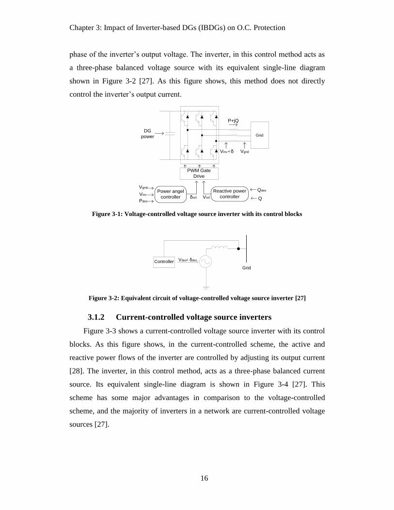
Chapter 3: Impact of Inverter-based DGs (IBDGs) on O.C. Protection
16
phase of the inverter’s output voltage. The inverter, in this control method acts as
a three-phase balanced voltage source with its equivalent single-line diagram
shown in Figure 3-2 [27]. As this figure shows, this method does not directly
control the inverter’s output current.
Grid
Vgrid
P+jQ
DG
power
PWM Gate
Drive
Power angel
controller
Reactive power
controllerVref.δref.
Vgrid
Pdes
Vinv
Qdes
Q
Vinv δ
Figure 3-1: Voltage-controlled voltage source inverter with its control blocks
Controller Vdes δdes
Grid
Figure 3-2: Equivalent circuit of voltage-controlled voltage source inverter [27]
3.1.2 Current-controlled voltage source inverters
Figure 3-3 shows a current-controlled voltage source inverter with its control
blocks. As this figure shows, in the current-controlled scheme, the active and
reactive power flows of the inverter are controlled by adjusting its output current
[28]. The inverter, in this control method, acts as a three-phase balanced current
source. Its equivalent single-line diagram is shown in Figure 3-4 [27]. This
scheme has some major advantages in comparison to the voltage-controlled
scheme, and the majority of inverters in a network are current-controlled voltage
sources [27].

Chapter 3: Impact of Inverter-based DGs (IBDGs) on O.C. Protection
17
Grid
Vgrid
I
DG
power
PWM Gate
Drive
controller
Active/Reactive
component
calculator
Id,des Vgrid
Iq
Id
Iq,des
Pdes
Qdes
3-ph/dqI
Vgrid
Figure 3-3: Current-controlled voltage source inverter with its control blocks
Controller
Grid
I θ
Figure 3-4: Equivalent circuit of current-controlled voltage source inverter [27]
3.2 Inverters’ O.C. protection
The termal time constants of power electronic switches are very small [28],
and the restriction on the temperature of semiconductor junction in these devices
makes them very sensitive to an excessive current [29]. Consequently, during the
grid faults, the inverter needs a protection mechanism which ceases its switching,
or restricts its current as quickly as possible, in order to protect it against severe
damage. This scheme can be either DG trip or software protection.
3.2.1 DG trip
In this protection scheme, the instantaneous or short-time delay O.C.
protection (function 50/51) disconnects the IBDG in the first few cycles or even
sub-cycles. In addition, the DG is also equipped with under-voltage protection
(function 27) [29]. The inverter’s disconnection is obtained simply by stopping
the switching signals [28]. The IBDGs in this category do not have LVRT
capability and cannot be integrated into the grids with LVRT requirements.

Chapter 3: Impact of Inverter-based DGs (IBDGs) on O.C. Protection
18
Figure 3-5 shows the RMS output current of a voltage-controlled voltage
source inverter with DG trip protection during a grid fault. In this figure, If
depends on the impedance between the IBDG and the fault location [30]. In case
of close faults, when If >1.25 p.u., the inverter will be ceased in less than half a
cycle [27] (e.g. 5 m.sec. [29]). In case of distant faults, when If >1.1 p.u., the
IBDG will be disconnected in less than 100 m.sec.
Time
Current
T0 T1
1 p.u.
If
Figure 3-5: Typical inverter’s RMS current during the fault (trip protection)
3.2.2 Current-limiting protection
In this protection scheme, instead of tripping the inverter, a current-limiting
mechanism is embedded in the inverter’s control loop and limits the inverter’s
output current to a predefined threshold during the grid’s disturbances. This
protection scheme protects the IBDG’s semi-conductor switches from excessive
currents and facilitates LVRT by avoiding DG trip. Several methods to achieve
the current-limiting protection have been introduced in [31]-[32]. Regardless of
the limiting method, an inverter with the current limiting protection has a fault
response similar to that in either Figure 3-6(a) or Figure 3-6(b).
Time
Current
T0 T1
1 p.u.
If
T2
(a)
Time
Current
T0 T1
1 p.u.
If
T2
If,tr
(b)
Figure 3-6: Typical inverter’s RMS current during the fault (current limiting protection)

Chapter 3: Impact of Inverter-based DGs (IBDGs) on O.C. Protection
19
As these figures show, the inverter’s response can be divided into three
periods: transient (T0<t<T1), the steady-state (T1<t<T2) and trip (t>T2). In both
cases, steady-state fault current could be as high as 115% of its rated current (in
some cases, 150-200%). After T2, the inverter’s under-voltage protection
disconnects the inverter from the grid. According to IEEE1547 [4], the period
between T0 and T2 could be up to .16 sec (9.6 cycles).
The only difference between Figure 3-6 (a) and Figure 3-6 (b) is that in the
latter, the transient fault current is higher than its steady-state value ( could be
up to 200% of the rated current.) However, this transient fault current lasts for
only about 1 cycle; i.e., in Figure 3-6(b), T1-T0<17m.sec. In other words, in such
inverters, output current reaches to 2 p.u. in the first cycle after the fault, and then
is limited to 1.15 p.u. for some cycles and then is disconnected. Normally, the
voltage-controlled voltage source inverters show such response. In contrast, for
inverters with fault responses similar to that in Figure 3-6(a), when the fault
occurs, a few cycles are required for the inverter to reach its current limit of 1.15
p.u., and then the current remains at this level for some cycles, and after that, the
inverter is disconnected by its under-voltage protection. Normally, current-
controlled voltage source converters show such responses.
3.3 Contribution of IBDGs to fault current
IBDGs with DG trip protection barely impact on the O.C. protection. Indeed,
the contribution time window in these DGs is too short to interfere with the
distribution system’s protection. For example, in [13], the short circuit test result
for a typical 1 kW inverter is provided. In this test, the inverter’s maximum peak
current was approximately 5 times the pre-fault peak current (If=5 p.u.). However,
the inverter’s operation was ceased in 0.1 cycle (T1-T2=1.6 m.sec.) Also, in [13] a
manufactured inverter fault current is provided in which the peak fault current
reaches 3 times its value during the pre-fault period but lasts for only 4.25 m.sec.
The comparison of these time windows and the typical response times of the O.C.
devices (Figure 2-3) reveals that these DGs cannot impact on the O.C. protection
coordination.

Chapter 3: Impact of Inverter-based DGs (IBDGs) on O.C. Protection
20
In case of IBDGs with the current-limiting protection, although the
magnitude of the current is limited, it can last for several cycles. In such DGs, the
control system intentionally restricts the output current to a pre-set value.
For example, in [33], two commercial 3-phase 480V 30kW solar inverters
were tested. Both inverters had fault responses similar to Figure 3-6(b). Under the
3-phase to ground fault at the inverters’ terminals, the first inverter produced a
current about 1.8 p.u. for the first cycle after the fault occurred, and then the
current decreased to its rated value. Finally, the inverter shut down 9 cycles after
the fault (See Figure 3-7). Likewise, the second inverter produced a current of
around 1.2 p.u. in the first cycle after the fault occurred and then, the current
decreased to almost its rated value and finally, inverter shut down after 6 cycles
(See Figure 3-8).
Figure 3-7: Response of a commercial inverter with current limiting protection to 3-phase
fault [33]
Figure 3-8: Response of another commercial inverter with current limiting protection to 3-
phase fault [[33]
Figure 3-9 provides another example showing the experimental result of the
short circuit test for a software-protected IBDG [31]. The result shows that the

Chapter 3: Impact of Inverter-based DGs (IBDGs) on O.C. Protection
21
inverter’s response to fault is similar to Figure 3-6 (a) and the current is restricted
to the pre-defined threshold more than twice the rated current.
Figure 3-9: Response of inverter with current limiting protection proposed in [31] to 3-phase
fault
3.4 Impact of DG on fuse-recloser coordination
As was discussed in the previous section, IBDGs with DG trip protection are
ceased too soon to impact on the protection system. As a result, in this section, the
focus is on IBDGs with current-limiting protection. In the following paragraphs,
the impact of the IBDG on the fuse-saving scheme is investigated as an example.
Finally, a mitigation strategy is proposed, and simulation results are presented.
As was briefly mentioned in section 2.2, in the fuse-saving scheme, when a
fault occurs on a lateral like the one shown in Figure 3-10, the recloser R first
operates one or more times based on its fast time-current curve. Most of the faults
in the distribution system are temporary and are cleared during fast reclosing
actions [34]. If the fault is quasi-permanent, the fuse F is supposed to clear the
fault instead. The time-delayed operation of the recloser will occur if the fuse fails
to interrupt the fault current. Consequently, in case of a permanent fault, the fuse
is set to melt between the fast and time-delayed operation of an automatic
recloser. Applying the fuse-saving scheme has two main advantages [35]:
1. No interruption in power delivery occurs due to temporary faults.
2. Fuse burning and replacement are needed only if the fault is quasi-
permanent.

Chapter 3: Impact of Inverter-based DGs (IBDGs) on O.C. Protection
22
Grid R
F
Fault
Figure 3-10: Fuse-Recloser protection scheme in distribution feeders
For proper coordination, the fuse and recloser curves are selected and set in a
way that for all possible faults, the fuse and recloser fault currents remain within
the limit shown in Figure 3-11.
Fast curve
Time-delayed
curve
Current
Time (s)
Fuse
Current
Limits
B
A
Figure 3-11: Fuse-Recloser time-current characteristic curves
Nonetheless, the insertion of a DG changes the fault current experienced by
the fuse and recloser. For example, for low-impedance faults, adding a DG to the
system may increase the fault current experienced by the fuse. This result pushes
the fuse current to the right side of point B as shown in Figure 3-12. In this case,
the fuse melts either simultaneously or faster than the operation of the recloser,
and an undesirable permanent interruption occurs on the lateral, even for
temporary faults.
Current
B
B’
Time (s)
Decreas in fuse
operation time
Increase in
fuse current
Figure 3-12: Impact of DG on operation of protection system under low impedance fault
situation

Chapter 3: Impact of Inverter-based DGs (IBDGs) on O.C. Protection
23
For further analysis, Figure 3-13 shows an equivalent circuit for a system
with an inverter-based DG when a fault occurs downstream of the DG. In this
figure, the network upstream of the distribution substation is modeled as an
equivalent ideal voltage source E, and an equivalent impedance Znet. In this
model, the loads are neglected (considered as open circuits) during the fault. In
addition, Z1 and Z2 are feeder impedances from the substation to the PCC, and
from the PCC to the fault location, respectively. R represents the recloser, and Rf
is the fault resistance.
Zn
et
R
Rf
Network
equivalent IDG
fuse
E
If
Ir PCCZ2
DS
substation
Z1
Figure 3-13: Equivalent circuit of a distribution system with inverter-based DG, during a
downstream fault.
In this system, the three-phase short circuit per-unit current before
implementing the DG can be estimated as
1 2
r f
net f
EI I
Z Z Z R
(3-1)
After adding the DG, the currents through the recloser and fuse can be obtained as
2
1 2 1 2
f
r DG
net f net f
R ZEI I
Z Z Z R Z Z Z R
(3-2)
1
1 2 1 2
netf DG
net f net f
Z ZEI I
Z Z Z R Z Z Z R
(3-3)
At point B of Figure 3-11, where a low-impedance fault occurs near the PCC
(Rf+Z2≪Znet+Z1), the recloser and fuse currents can be approximated as
1 2
r
net f
EI
Z Z Z R
(3-4)
1 2
f DG
net f
EI I
Z Z Z R
(3-5)

Chapter 3: Impact of Inverter-based DGs (IBDGs) on O.C. Protection
24
From (3-4) and (3-5), it can be concluded that adding a DG increases the fuse
current in low-impedance faults, while the fault current experienced by the
recloser is almost constant. Thus, in this case, the fuse may operate faster than the
recloser, leading to a coordination failure. Suppose that before adding the DG,
Point B of Figure 3-11 is reached for a fault with resistance Rf1. After adding the
DG, point B will be reached for a fault with resistance Rf2, where necessarily Rf2 >
Rf1. Consequently, fuse-recloser protection cannot be applied for faults with
resistances between Rf1 and Rf2.
On the other hand, for high-impedance faults (Rf+Z2≫ Znet+Z1) the recloser
and fuse current can be estimated as
1 2
r DG
net f
EI I
Z Z Z R
(3-6)
1 2
f
net f
EI
Z Z Z R
(3-7)
(3-6) and (3-7) show that for high-impedance faults (like that represented by
point A of Figure 3-11), the current experienced by the recloser is reduced after
adding the DG, while the fuse current is almost constant. Under this condition, the
fuse operation time remains constant, but the recloser time-delayed operation
occurs with an additional delay. However, this delay will not cause
miscoordination since the fuse operates sooner than the recloser’s time-delayed
operation.
Furthermore, analysis of a fault occuring upstream to the DG was also
conducted in a similar way. It was found that the situation matched closely with
that of a downstream fault. This finding means the location of the faults does not
play a significant role in the fuse-recloser coordination. Instead, the DG current
and fault impedance will have more impact on the coordination. Moreover,
compared to the situation of a high-impedance fault, where the coordination is
usually maintained, a low-impedance fault tends to cause more problems. For this
reason, low-impedance faults are considered in the rest of this work.
Another important factor to consider is the inverter’s power factor. The
provision of reactive power has been considered as one of the most important

Chapter 3: Impact of Inverter-based DGs (IBDGs) on O.C. Protection
25
ancillary services offered by inverter-based DGs [36]-[38]. However, if not
controlled and coordinated properly, this reactive power injection may worsen the
protection miscoordination. Consider a low-impedance downstream fault as an
example, where the fuse current has two parts as shown in (3-5). In active power
injection from the DG, the first part of the fuse current 1 2net f
E
Z Z Z R is
about 90o out of phase with the PCC voltage, while the second part (the DG
current) IDG is forced to be in phase with the PCC voltage. As a result, the two
terms have a phase shift of around 90o, and the relationship in (3-8) can be
obtained:
1 2 1 2
DG DG
net f net f
E EI I
Z Z Z R Z Z Z R
(3-8)
However, in reactive power injection from a DG, both terms in the fuse
current (1 2net f
E
Z Z Z R and IDG) are about 90
o out of phase with the PCC
voltage. Consequently, the relationship in (3-9) is obtained:
1 2 1 2
DG DG
net f net f
E EI I
Z Z Z R Z Z Z R
(3-9)
For further illustration, Figure 3-14 shows the vector diagram of the above
voltages and currents (note that the direction of the DG current is to the PCC).
Figure 3-14(a) and Figure 3-14(b) show that the fault current through the fuse is
larger when the DG provides reactive power. This result means that in comparison
to active power injection, reactive power injection worsens the fuse-recloser
coordination situation.

Chapter 3: Impact of Inverter-based DGs (IBDGs) on O.C. Protection
26
EVPCC
IDG.
Ir If
Ir
If
IDG.
VPCC
E
(a) (b)
Figure 3-14: Voltage and current vector diagram of: a) DG provides active power, b) DG
provides reactive power.
As was mentioned in Chapter 1, one aspect of LVRT capability required by
grid codes is that the DGs support the grid voltage by injecting reactive power
during/after the fault, while another aspect is that the DGs support the continuity
of service by providing active power. The above discussion showed how these
two aspects could possibly conflict with each other.
3.5 The proposed strategy
To mitigate the impact of the DG on the fuse-recloser coordination, a simple
and effective DG current control strategy is proposed in this section.
In common practice, the inverter’s current during a low-impedance fault is
restricted up to twice its nominal current [39]. The ideal way to eliminate the
impact of the DG on the protection system is to detect the fault and trip all the
converters in that protection zone. However, this method conflicts with the LVRT
capability required by some distribution grid codes. As well, converters are unable
to differentiate between fault conditions and short-term disturbances such as load
switching. Therefore, converter tripping in all abnormal conditions may lead to
unnecessary power-delivery interruptions.
One way to ride through short-term disturbances and avoid excessive
nuisance tripping is to introduce an allowed time delay, as is shown in Table 3-1.
If the abnormal condition remains after the delay, according to IEEE std. 1547
[4], the converter should be tripped and then reconnected 5 minutes after the
system has returned to its normal condition.

Chapter 3: Impact of Inverter-based DGs (IBDGs) on O.C. Protection
27
Table 3-1: IEEE std. 1547 required response to abnormal voltage conditions [4].
Voltage at PCC Maximum tripping time (sec)
V<50% .16
50%<V<88% 2
88%<V<110% Normal operation
110%<V<120% 1
137%<V .16
Currently, the fast automatic reclosers operate in less than 6 cycles after fault
occurrence, so the above time delays may not be effective; i.e., during the
reclosing, the DG still contributes to the arching fault. In addition, decreasing
these delays may cause excessive nuisance tripping due to short-term
disturbances.
One idea to simultaneously solve the miscoordination problem and ride
through short-term disturbances is to reduce the converter current according to the
severity of the abnormality instead of completely blocking the converter. In this
case, the converters near the fault location, which will produce the greatest impact
on the protection system, experience the most voltage deviation from the normal
boundaries and should significantly decrease their fault current contribution. On
the other hand, the more distant DG units, which have no substantial effect on the
protection system, can continue their power delivery.
To implement the above-mentioned current-control strategy according to the
DG terminal voltage, the DG’s reference current can be determined as in (3-10)
.
. max
0.88 . .
0.88 . .
desired
ref PCC
PCC
n
ref PCC PCC
PI for V p u
V
I kV I for V p u
(3-10)
where Iref is the converter reference current, Imax is the maximum output current
that happens at VPCC =0.88p.u. (the lower boundary for normal operation
according to Table 3-1), VPCC is the rms voltage at the DG connection node,
Pdesired is the output desired power, and k and n are constants to be determined.

Chapter 3: Impact of Inverter-based DGs (IBDGs) on O.C. Protection
28
Generally, the value of n determines the sensitivity of the control scheme to a
voltage change. A larger value of n leads to more obvious output current
reduction with a voltage sag. However, a too large n will cause the control scheme
to be overly sensitive to even a small voltage disturbance. Therefore, n=3 is
selected in this work. Once the value of n is chosen, the coefficient k can be
determined in such a way that the reference current in (3-10) remains a continuous
function around VPCC =0.88 p.u.; i.e., k can be obtained from (3-11), which gives
k=1.4674 when n=3.
max 1
max
(0.88)0.88 (0.88)
n desired desired
n
P Pk I k
I
(3-11)
Figure 3-15 shows the flow chart illustrating the reference current
determination procedure.
. . max
n
ref PCCp uI kV I.
desired
ref
PCC
PI
V
Vpcc Measured
Inverter
Vpcc > 0.88p.u.No
Yes
Figure 3-15: Proposed strategy to determine inverter reference current
3.6 Simulation results
In order to illustrate the impact of an IBDG on the coordination and to
demonstrate the ability of the proposed method to mitigate this impact, several
simulations were conducted. The results of these simulations are presented in
following sections.
3.6.1 Performance during low-impedance faults
To investigate the ability of the proposed strategy to maintain fuse-saving
coordination, a 13-Node Test Feeder system (see Figure 3-16) [40] was

Chapter 3: Impact of Inverter-based DGs (IBDGs) on O.C. Protection
29
constructed by using MATLAB/SIMULINK. A recloser was mounted at the
substation, and an inverter-based DG was connected at node 645. The simple
current-controlled voltage source inverter model in [28] is used in this work. The
DG’s effect on the coordination between the recloser and the fuse on 645-646 was
studied for faults in the middle of 645-646. Figure 3-17 shows the time-current
characteristic curves of the recloser and fuse used in simulations.
In the simulated system, point B occurs for a fault resistance of 0.01 Ohm,
and point A occurs for a fault resistance of 11.5 Ohms. In other words, the fuse
and recloser operate properly for fault resistances between 0.01 to 11.5 Ohms. For
faults with resistances lower than 0.01 Ohm, the fuse operates faster than the
recloser, and the use of the fuse-saving scheme is not feasible. Note that normally,
protection engineers try to select the fuse and recloser so that the operation point
for a solid fault is located on the left side of point B. However, sometimes either
marginal coordination cannot be avoided or the original operation point can slide
to the right by network expansion. Therefore, in this study, we considered the
worst condition.
Figure 3-16: IEEE 13-Node test feeder system [40]
Figure 3-17: Fuse-recloser coordination in the simulated system
646 645 632 633 634
650
692 675611 684
652
671
680

Chapter 3: Impact of Inverter-based DGs (IBDGs) on O.C. Protection
30
Figure 3-18 shows the consequence of adding a DG at different penetration
levels (Penetration level=PDG/Pload ×100) on the O.C. coordination when a 0.01
Ohm fault occurs. As Figure 3-18 reveals, after adding a DG even at low
penetration levels, the fuse operates faster than the recloser, and the protection
coordination is lost.
Figure 3-18: Difference between fuse and recloser operation time after adding DG for 0.01
Ohm fault
This problem will appear in situations with even higher fault resistances.
Figure 3-19 shows that miscoordination occurs in a fault with 0.1 Ohm resistance
in the presence of a DG at high penetration levels. As this figure reveals, although
the fault resistance is higher than the one in point B, adding a DG at penetration
levels higher than 70% will cause miscoordination.
Figure 3-19: Difference between fuse and recloser operation time after adding DG for 0.1
Ohm fault
To investigate the impact of reactive power injection on the protection
coordination and confirm the analysis of the previous sections, the DG control
scheme was modified so that the DG provided active power during normal
conditions, but injected a fully reactive current when it experienced a voltage sag
(Vpcc<0.88p.u.). Figure 3-20 shows the PCC’s voltage magnitude and the DG

Chapter 3: Impact of Inverter-based DGs (IBDGs) on O.C. Protection
31
current phase angle for a fault occurring at t=0.25 sec. Figure 3-21 shows the
difference between fuse and recloser fast operation times under this control
scheme, for a 0.01 Ohm fault.
The comparison between Figure 3-18 and Figure 3-21 reveals that the fuse
melted sooner when the DG injected reactive power. This impact occurred even in
situations with higher fault resistances. Figure 3-22 shows that with reactive
power injection, miscoordination occurred for Rf=0.1 Ohm even at low
penetration levels like 30% (compared to 70% in Figure 3-18). In addition, Figure
3-23 shows that reactive power injection caused miscoordination in 0.2 Ohm
faults for penetration levels higher than 75%. Note that no miscoordination
occurred for 0.2 Ohm faults at any penetration level when the DG provided only
active power. This example shows how reactive power generation could possibly
degrade the reliability even though the original objective was to increase the
service reliability.
Finally, Figure 3-24 shows the effect of the proposed control scheme on the
protection coordination. As this figure shows, this control scheme successfully
solved the miscoordination in low-resistance faults due to DG injection. This
figure also reveals that with the proposed control scheme, the DG penetration
level had almost no effect on low impedance faults because PCC voltage is very
low under a low-impedance fault (see Figure 3-25), and as shown in Figure 3-26,
the DG output current decreased to almost zero with the proposed method. As a
result, the protection devices did not experience any difference between this
system with a DG and the previous system with no DG, and the coordination was
maintained (see Figure 3-27). Note that this result contrasts with the case in which
traditional control was applied to the inverter. In this case, during voltage sags,
the traditional control increased the inverter current until it reached the pre-set
current threshold (Ith), which is normally set to 1.3~2 times the Irated current.
Therefore, the fuse current was increased, and, consequently, miscoordination
occurred.

Chapter 3: Impact of Inverter-based DGs (IBDGs) on O.C. Protection
32
Figure 3-20: Intentional phase shift in DG current during voltage sag to support voltage.
Figure 3-21: Difference between fuse and recloser operation time for 0.01 Ohm fault with
pi/2 phase shift in inverter current.
Figure 3-22: Difference between fuse and recloser operation time for 0.1 Ohm fault with pi/2
phase shift in inverter current.
Figure 3-23: Difference between fuse and recloser operation time for 0.2 Ohm fault with pi/2
phase shift in inverter current.

Chapter 3: Impact of Inverter-based DGs (IBDGs) on O.C. Protection
33
Figure 3-24: Difference between fuse and recloser operation time for 0.01 Ohm fault with
inverter current reduction control.
Figure 3-25: PCC voltage for 0.01 Ohm fault with DG at 30% penetration level.
Figure 3-26: DG output current for 0.01 Ohm fault with DG at 30% penetration level.
Figure 3-27: Fuse current for 0.01 Ohm fault with DG at 30% penetration level.
In the next step, in order to show the effectiveness of the proposed strategy in
multiple DG cases, two DG units were used in the test system. One was
implemented at Node 634 with a capacity equal to 20% of the total load of the

Chapter 3: Impact of Inverter-based DGs (IBDGs) on O.C. Protection
34
system. The other was installed at Node 675 with a capacity equal to 60% of the
total load of the distribution system. Their effect on the coordination between the
recloser and the fuse on 645-646 was studied for a 0.1 Ohm fault occuring in the
middle of 645-646. Figure 3-28 and Figure 3-29 show these inverters’ output
currents when controlled by the proposed strategy. In addition, Figure 3-30
demonstrates the fuse current in both the traditional and current-restricting
strategies. As this figure reveals, in contrast to the traditional control, the
proposed strategy successfully kept the fuse current below the margin, and
consequently maintained the coordination even when multiple DGs with high
penetration at different locations were used.
Figure 3-28: Output current of inverter installed at Node 634.
Figure 3-29: Output current of inverter installed at Node 634.
Figure 3-30: Fuse current for.1 Ohm fault with DG units at Nodes 634 and 675.

Chapter 3: Impact of Inverter-based DGs (IBDGs) on O.C. Protection
35
3.6.2 Performance during high impedance faults
The converter’s operation controlled by the proposed strategy during
medium- and high-impedance faults was studied in this stage of the simulations.
In the first case, three DGs at a 30% total penetration level (10% each) were
implemented on Nodes 633, 645 and 675, and a 2-Ohm fault was simulated in the
middle of 645-646. Figure 3-31 shows the converters’ output current. This figure
reveals that the more distant converters experienced lower voltage sags and,
consequently, provided more current during a fault.
Figure 3-31: Output current of inverters for 2-Ohm fault in the middle of 645-646.
In the second case, a DG was installed at Node 634 with a capacity equal to
the spot load at this node, and an 8-Ohm fault was simulated from 0.2 sec. to 0.3
sec. in the middle of Nodes 645-646. Figure 3-32 shows the inverter output power
in this situation. Figure 3-33 shows the PCC voltage, and Figure 3-34 shows the
fuse current. According to these results, the converter with the proposed control
strategy can successfully rode through high impedance or distant faults without
losing its power delivery capability, and improved the voltages of the local nodes
without having any impact on the protection system.
Figure 3-32: Inverter output power for 8-Ohm fault in the middle of 645-646.

Chapter 3: Impact of Inverter-based DGs (IBDGs) on O.C. Protection
36
Figure 3-33: PCC voltage for 8-Ohm fault in the middle of 645-646.
Figure 3-34: Fuse current for 8-Ohm fault in the middle of 645-646.
3.6.3 Performance during non-fault disturbances
To test the performance of the proposed control method under a network
disturbance other than a fault condition, a distribution feeder with an induction
motor load was simulated. The single line diagram of this feeder is shown in
Figure 3-35. The distribution system parameters are listed in Table 3-2: Test
system parameters. The substation was modeled by a three-phase balanced
voltage source and equivalent impedance, and the line was modeled by series R-L
branches. As shown in Figure 3-35, this feeder had five laterals, and a recloser
was mounted at its middle. F is an 80A fuse, and R is a recloser in conjunction
with an IEEE extremely inverse relay, which is the most suitable option for fuse-
saving [41].
Figure 3-36 shows the fuse’s time-current curve superimposed on the
recloser’s curve. Point A is the fuse operation point for a three-phase fault at the
beginning of L5 before adding an inverter-based DG. Since A is to the left of B,
the recloser operates faster than the fuse, and F will be saved in case of temporary
faults at L5. In contrast, after adding a 1-MW inverter-based DG, the fuse’s

Chapter 3: Impact of Inverter-based DGs (IBDGs) on O.C. Protection
37
operation point moves from A to C, and fuse saving is no longer practical unless
the proposed control strategy is utilized.
R
L2
L1L3
L4
L5
NET
Substation
IM
Inverter
F
Figure 3-35: A distribution network with fuse-saving protection.
Table 3-2: Test system parameters
Parameter Value
Main trunk overhead line length 12.00 km
Main trunk underground cable length 10.85 km
Substation short-circuit level 305 MVA
Substation equivalent impedance (including
substation transformer)
Z+= 0.035 + j2.05 Ω
Z0= 0.053 + j2.161 Ω
Overhead line type 336.4 ACSR
Underground cable type 500Al XLPE 25kV
DBUR
Substation grounding resistance .15Ω
Total active power load 8.79 MW
Table 3-3: Induction machine’s parameters
Parameter Value
Nominal power 1MW
Stator impedance 0.01965+ j0.0397 p.u.
Rotor impedance 0.01909+ j0.0397 p.u.
Mutual inductance 1.354 p.u.
Inertia constant 0.5 s
Friction factor 0.05479 p.u.
Pole pairs 2

Chapter 3: Impact of Inverter-based DGs (IBDGs) on O.C. Protection
38
Figure 3-36: A distribution network with fuse-saving protection.
To study the response of an inverter-based DG controlled by the proposed
strategy during none-fault disturbances, the starting of a 1-MW induction motor
(IM) was considered and simulated. The induction motor parameters are listed in
Table 3. As demonstrated in Figure 3-37, only a 5% reduction occurs in the DG
output power. Such a reduction barely decreases the voltage at the PCC. As
Figure 3-38 reveals, the time-voltage curves at the motor terminal match for both
the traditional and current-restricting control strategies. Finally, Figure 3-39
shows the inverter output current during this transient. As can be seen, the current
limiting control is not enabled, as the inverter terminal voltage is higher than
0.88p.u.
Figure 3-37: DG output power during motor starting for both traditional and proposed
control strategies.
Figure 3-38: Voltage at terminals of IM during motor starting for both traditional and
proposed control strategies.

Chapter 3: Impact of Inverter-based DGs (IBDGs) on O.C. Protection
39
Figure 3-39: Inverter output current during the motor starting transient.
These simulation results not only show that the proposed control strategy is
appropriate for fuse saving, but also demonstrate the robustness of this strategy
against none-fault disturbances. In other words, this strategy reduces inverter
output only during low-impedance faults when fuse-burning is possible. In
contrast, the DG output power remains almost constant for other network
disturbances, and, consequently, it does not cause further voltage reduction.
3.7 Conclusion
In this chapter, the contribution of IBDGs to the fault current was analyzed,
and their impact on O.C. coordination was investigated. For this reason, IBDGs
were categorized as either current-limiting protected or DG tripping ones. Base on
this categorization, the following conclusions have been made:
1. With DG trip protection, an IBDG’s fault current can reach to 5 p.u.
However, the IBDG is ceased in few cycles or even less than one
cycle. In this case, the contribution time window is too short to impact
the coordination.
2. With current-limiting protection, an IBDG’s fault current is limited to
a pre-defined threshold and can be continued until the operation of
undervoltage protection, which takes up to .16 sec. (9.6 cycles). The
threshold can be up to 2 p.u.
3. The simulations showed that IBDGs with current-limiting protection
may cause miscoordination when the protection devices are
marginally coordinated.

Chapter 3: Impact of Inverter-based DGs (IBDGs) on O.C. Protection
40
4. To mitigate the impact of IBDGs on coordination, a strategy was
proposed in which the threshold was not fixed but adjusted
dynamically based on the PCC voltage. The simulation results showed
that by using the proposed control strategy, the inverter’s current was
limited significantly when a fault happened near the PCC. As a result,
the IBDG had no contribution to the fault and could not impact on the
coordination. Moreover, when this strategy was used, when non-fault
disturbances or distant faults occurred (on which the DG had no
impact), the IBDG operated normally.

Chapter 4: Impact of Synchronous-Machine DGs (SMDGs) on O.C. Protection
41
Chapter 4
Impact of Synchronous-Machine DGs
on O.C. protection
As was mentioned in Chapter 1, DGs can be made to respond in two ways
during a fault. First, the DG can be disconnected quickly after the fault, and as a
result, the DG has no impact on the O.C. protection. Second, the DG can be
required to ride through the low voltages. In previous chapters, it was shown that
DG units with the LVRT approach can negatively impact the distribution
protection system and result in serious protection malfunctions such as false
tripping, relay desensitization, and miscoordination between the main and back-up
protection devices [42]-[46]. In this chapter, the focus is on the contribution of
SMDGs to the fault current and on mitigating their impact on the O.C. protection.
To mitigate the SMDG’s impact on the distribution protection system, several
methods have been proposed, which can be classified into the following
categories:
1. Limiting the DG capacity [47]-[49],
2. Modifying the protection system by using extra breakers or reclosers,
reconfiguring the network, or using distance or directional relays [50]-
[53],
3. Using adaptive protection [54]-[56], and
4. Utilizing Fault Current Limiters (FCLs) [57]-[59].
Although these methods are effective for mitigating the SMDG impact on the
protection system, they have some obvious disadvantages. Limiting the DG
capacity is not desirable since doing so also limits the DG penetration level.
Modifying the protection system is costly. Moreover, doing so requires utility
involvement and makes the protection procedure more complicated. Similarly,

Chapter 4: Impact of Synchronous-Machine DGs (SMDGs) on O.C. Protection
42
adaptive protection requires new communication infrastructures as well as fast
processing units. Finally, utilizing FCLs is also undesirable because of the
additional cost that using them imposes on utility or DG owners.
This chapter proposes a strategy to increase the SMDG’s compatibility with
the distribution network by mitigating the SMDG’s negative impact on the
protection system. The idea is to establish a method to restrict the DG’s
contribution to the fault current and, consequently, prevent its impact on the O.C.
protection. This idea can be implemented by either re-designing the generator and
considering large transient reactances, or controlling the machine’s field. In this
thesis, the latter approach is followed. The machine’s field can be controlled by
using either Automatic Voltage Regulator (AVR) or a field discharge circuit. In
this thesis, equipping the generator with a solid-state switch-based field discharge
circuit is considered as the strategy to mitigate the impact of the SMDG on the
O.C. protection. The solid line in Figure 4-1 shows the research direction in this
chapter. The main advantage of this approach is that the use of a filed discharge
circuit is self-contained (because utility involvement is not required) and less
expensive. As well, the machine reacts quickly to the operation of this circuit and
its use is a known practice with a good chance of being accepted by utility
regulators. The other options, utilizing FCLs or protection modification, as was
mentioned above, require utility involvement and are more expensive and
complex than field discharge. Furthermore, re-considering machine design is
challenging since any redesign will affect the machine’s overall performance and
also is not applicable to machines which are already in use.

Chapter 4: Impact of Synchronous-Machine DGs (SMDGs) on O.C. Protection
43
DG
Action
Disconect LVRT
Imp
act o
n
pro
tectio
n
Protection
ModificationFCL
Re-considering
Machine Design
Field
Control
AVRField
discharge
Figure 4-1: SMDG control strategies during grid fault
In the following sections, the operational reactances and time constants of a
SG are introduced, and the typical values for these parameters are provided. Next,
the response of these DGs to the grid faults is investigated. Then, case studies are
provided to demonstrate the potential impact of this type of DG on the O.C.
protection coordination. Next, the idea of utilizing the field discharge to mitigate
this impact is discussed, and a detailed analysis and a design procedure are
presented. In the next step, the case studies are re-considered by applying the field
discharge to the excitation system, and the effectiveness of the method is
demonstrated. Next, the impact of the field discharge on the voltage recovery in
the post-fault period is studied. Finally, the impact of the field discharge circuit on
the generator’s stability is investigated.
4.1 Operational reactances and time constants
Figure 4-2 shows a 3-phase synchronous machine with phase windings a, b,
and c on the stator, and field winding F and damper windings kd and kq on the
rotor. The mathematical relation between the voltages and currents of these
windings can be expressed in terms of self and mutual inductances and resistances
[60].

Chapter 4: Impact of Synchronous-Machine DGs (SMDGs) on O.C. Protection
44
aF
kdkq
c
b
Figure 4-2: Synchronous generator’s structure
The machine’s air gap is not uniform, so some inductances are functions of
the relative position Ѳ. In order to simplify the calculations, the stator parameters
can be transformed to a reference frame fixed on the rotor. In this way, two
fictitious windings with the same number of turns as those of the phase windings
are located on the direct- and quadrature-axes shown in Figure 4-3. Then their
currents are defined so that they produce the same mmf wave as that produced by
the actual phase currents.
F kd
kq
d
q
Figure 4-3: Equivalent synchronous machine with fictitious d- and q-axis windings
The flux linkage in the d-axis can be written in terms of the d-axis current and
the machine’s excitation voltage as follows [60]:
0 0
( ) ( )dd d F
x p G pi u
4(4-1)
where
' "
' "
0 0
(1 )(1 )( )
(1 )(1 )
d dd d
d d
T p T px p X
T p T p
(4-2)
A similar equation can be written for the q-axis
0
( )q
q q
x pi
(4-3)
where

Chapter 4: Impact of Synchronous-Machine DGs (SMDGs) on O.C. Protection
45
"
"
0
(1 )( )
(1 )
q
q q
q
T px p X
T p
(4-4)
In the above equations, ' ,dT ",dT '
0 ,dT "
0 ,dT",qT and
"
0qT are the machine’s time
constants, and as it will be shown in the next sub-section, the latter three constants
are used to express the machine’s response to the fault.
During a disturbance, the SG’s response can be divided into the sub-transient,
transient, and steady-state periods. The length of each period depends on the
above-mentioned time constants. As well, in each of these periods, the machine’s
equivalent circuit can be modelled by a voltage source and an operational
reactance. During sub-transient condition, the operational reactances are
' ""
' "
0 0
lim ( ) d dd p d d
d d
T TX x p X
T T
(4-5)
"
"
"
0
lim ( )q
q p q q
q
TX x p X
T
(4-6)
and during the transient condition, the operational reactance is as below
''
'
0
dd d
d
TX X
T
(4-7)
Finally, during the steady state operation of the synchronous machine, the
operational impedances are Xd(p=0) and Xq(p=0) which are Xd and Xq,
respectively. Table 4-1 shows the typical values for the SG time constants and
operational reactances, which play a role in the machine’s response to the grid
faults [61].

Chapter 4: Impact of Synchronous-Machine DGs (SMDGs) on O.C. Protection
46
Table 4-1: Comparison of impedance estimation method with data-based single-point
problem [61]
Parameter
Typical range
Round rotor Salient rotor
1-2.5 p.u. 1-2 p.u.
1-2.5 p.u. .6-1.2 p.u.
.2-.35 p.u. .2-.45 p.u.
.12-.25 p.u. .15-.25 p.u.
.1-.25 p.u. .2-.8 p.u.
1-1.5 s 1.5-2 s
.03-.1 s .03-.1 s
4.2 Synchronous generator’s fault current
In this section, the SG’s response to the short circuit at its terminals is
studied. Amongst all types of faults, the three-phase solid fault at the terminals
results in the highest fault current and, consequently, is the worst case. Besides, its
calculation is simpler than those for the other types of faults due to its symmetry.
Thus, in following paragraphs, this type of short circuit will be studied. Also, the
rotor’s speed is considered constant so that the machine’s equations can be solved
analytically.
For a three-phase solid fault at the generator’s terminals, the machine’s d- and
q-axis currents and, subsequently, the phase currents, are obtained by solving the
following differential equations:
0
0
d d q a d
q q d a q
u p R i
u p R i
(4-8)
By replacing ψd and ψq with 4(4-1) and (4-2), respectively, and calculating the
initial conditions by using the steady state analysis of the pre-fault, (4-8) can be

Chapter 4: Impact of Synchronous-Machine DGs (SMDGs) on O.C. Protection
47
analytically solved. Briefly, the SG’s current at phase a in case of a 3-phase solid
fault at the terminals can be expressed as follows:
' "
"
0 0' " '
0 0 0" " " "
0 0" "
1 1 1 1 1( )
1 1 1 1cos cos(2 )
2 2
1 1 1 1( )
2
d d
a a
q
t t
T T
a mq
d d d d d
t t
mq mqT T
d q d q
t
T mdmd
q q q d
i U e e cos tX X X X X
U Ue e t
X X X X
UU e sin t
X X X X
0"
0 0" "
1sin
1 1sin(2 )
2
a
a
t
T
q
t
Tmd
d q
eX
Ue t
X X
(4-9)
To obtain the currents at phases b and c, θ0 should be replaced by (θ0-2π/3) and
(θ0-4π/3), respectively.
As (4-9) reveals, the fault current consists of three components: the decaying dc,
the ac at the fundamental frequency, and the decaying ac at twice the fundamental
frequency. The ac component at the fundamental frequency is the most important
component in terms of the O.C. protection because most of the O.C. relays filter
the other components and operate based on only the 60Hz component of the fault
current. This component itself consists of three parts.
1. Sub-transient part
"
"
. 0 0" '
0 0"
1 1( )
1 1( )
d
q
t
T
sub mq
d d
t
T
md
q q
i U e cos tX X
U e sin tX X
(4-10)
This part is a decaying part of the 60Hz component with sub-transient time
constants in the range of .03-.1 sec. (see Table 4-1). Therefore, this component
disappears 2~3 cycles after the fault occurrence. In order to find a typical RMS
value for this part, the RMS of (4-10) can be approximated as follows (by
ignoring the machine’s saliency):

Chapter 4: Impact of Synchronous-Machine DGs (SMDGs) on O.C. Protection
48
"
., "
1d
t
T
sub RMS
d
i eX
(4-11)
After inserting the typical values from Table 4-1 into (4-11), it can be concluded
that the maximum RMS of the generator’s sub-transient 60Hz component is in the
range of 4~8 p.u.
2. Transient part
'
. 0 0'
1 1( )d
t
T
tran mq
d d
i U e cos tX X
(4-12)
This part is also decaying with a transient time constant in the range of 1-2 sec.
(see Table 4-1). Thus, this component lasts for several cycles after the fault
occurrence. In order to find a typical RMS value for this part, the RMS of (4-12)
can be approximated by the following equation:
'
., '
1d
t
T
tran RMS
d
i eX
(4-13)
After inserting the typical values from Table 4-1 to (4-13), it can be concluded
that the maximum RMS of the generator’s transient 60Hz component is in the
range of 3~5 p.u.
3. Steady-state part
. . 0 0 0 0
1 1( ) ( )s s mq md
d q
i U cos t U sin tX X
(4-14)
This part does not decay, appears after the transient period, and lasts until the fault
is cleared. In order to find a typical RMS value for this part, the RMS of (4-14)
can be estimated by using the following equation:
. .,
1s s RMS
d
iX
(4-15)
After inserting the typical values from Table 4-1 into (4-15), it can be concluded
that the maximum RMS of the generator’s steady-state 60Hz component could be
less than 1 p.u.

Chapter 4: Impact of Synchronous-Machine DGs (SMDGs) on O.C. Protection
49
For further illustration, the current waveform of a typical generator in case of
a 3-phase solid fault at the terminals at t=.2 sec. is demonstrated in Figure 4-4.
(a)
(b)
Figure 4-4: Typical synchronous generator’s fault current: (a) Complete waveform, (b) first 18 cycles
It is useful to compare the synchronous generator’s response to the grid fault
with the typical characteristics of O.C. protection devices. By comparing Figure
4-4 and Figure 2-3, and considering the generator’s typical time constants
available in Table 4-1, it can be concluded that the generator’s sub-transient
response coincides with the operation of the instantaneous and extremely inverse-
time relays, while the transient response of the generator (when the generator’s
output is 3~5 p.u.) coincides with the operation of the short-time delay and the
inverse and very inverse-time O.C. relays which provide the majority of the O.C.
protection.
4.3 Case studies
The main aim of this sub-section is to illustrate the impact of a SMDG on the
O.C. protection coordination. Two case studies are provided. In the first one, the
impact of a SMDG on the main and the back-up protection coordination is
analyzed. In the second one, the impact of a SMDG on the fuse-saving scheme is
described.
4.3.1 Impact on the main and back-up protection coordination
In this section, the contribution of a SMDG to 3-phase faults in the
distribution system is studied, and the SMDG’s impact on the O.C. protection is
analyzed. To do so, a sample 25 kV distribution system with its single line
diagram shown in Figure 4-5 was simulated. In this system, the upstream network
is represented by a Thevenin equivalent of a voltage source and a series
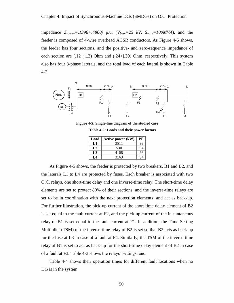
Chapter 4: Impact of Synchronous-Machine DGs (SMDGs) on O.C. Protection
50
impedance Zsource=.1396+.4800j p.u. (Vbase=25 kV, Sbase=100MVA), and the
feeder is composed of 4-wire overhead ACSR conductors. As Figure 4-5 shows,
the feeder has four sections, and the positive- and zero-sequence impedance of
each section are (.12+j.13) Ohm and (.24+j.39) Ohm, respectively. This system
also has four 3-phase laterals, and the total load of each lateral is shown in Table
4-2.
S
DG
Net. B1 B2
F1 F2F3
L1 L2 L3 L4
A B C DTs
F4
80% 20%80% 20%
TIG
Figure 4-5: Single-line diagram of the studied case
Table 4-2: Loads and their power factors
Load Active power (kW) PF
L1 2511 .93
L2 530 .94
L3 4108 .93
L4 3163 .94
As Figure 4-5 shows, the feeder is protected by two breakers, B1 and B2, and
the laterals L1 to L4 are protected by fuses. Each breaker is associated with two
O.C. relays, one short-time delay and one inverse-time relay. The short-time delay
elements are set to protect 80% of their sections, and the inverse-time relays are
set to be in coordination with the next protection elements, and act as back-up.
For further illustration, the pick-up current of the short-time delay element of B2
is set equal to the fault current at F2, and the pick-up current of the instantaneous
relay of B1 is set equal to the fault current at F1. In addition, the Time Setting
Multiplier (TSM) of the inverse-time relay of B2 is set so that B2 acts as back-up
for the fuse at L3 in case of a fault at F4. Similarly, the TSM of the inverse-time
relay of B1 is set to act as back-up for the short-time delay element of B2 in case
of a fault at F3. Table 4-3 shows the relays’ settings, and
Table 4-4 shows their operation times for different fault locations when no
DG is in the system.

Chapter 4: Impact of Synchronous-Machine DGs (SMDGs) on O.C. Protection
51
Table 4-3: Relays’ settings
Inverse-time relay Short-time delay element
Ipick-up (A) TSM Ipick-up (A) Operation time (s)
B1 320 .2775 4440 .1
B2 240 .1447 4030 .1
Table 4-4: Fault currents and relays’ operation times
Fault IR1(A) TR1(s) IR2(A) TR2(s)
F1 4440 .1 - -
F2 4038 .745 4030 .1
F3 4190 .73 4187 .1
F4 3996 .75 4002 .35
When the SMDG is added in the substation, the SMDG’s contribution to the
fault increases the fault current which flows through the protection devices. This
increase may cause miscoordination between B1 and B2. As an example, consider
a fault at F3. When there is no DG, the current through B2 is 4187A which leads
to the operation of its instantaneous relay, while the current through B1 is 4190A,
which results in the operation of its inverse-time relay. However, when the DG is
added, if it increases the fault current at F3 above 4440A (the pick-up current of
B1’s instantaneous relay), both B1 and B2 operate simultaneously, and the whole
feeder is de-energized. Figure 4-6 shows the fault current at F3 for the case with
5MW SMDG with parameters tabulated in Table 4-5. As this figure shows, for
SMDGs with higher capacities, the coordination between B1 and B2 will be lost.
As an example, Figure 4-7 shows how a 6.5 MW SMDG moves the protection
operation points from “A” to “B” and causes miscoordination.
Table 4-5: Operational constants of simulated synchronous machine [62]
Time constant (s) Operational reactance (p.u.)
Td0'=9.00000 Xd=1.55000
Td'=2.03226 Xq=1.40000
Td0"=.03000 Xd'=.35000
Td"=.01543 Xd"=.18000
Tq0"=.04000 Xq"=.18000
Tq"=.01711

Chapter 4: Impact of Synchronous-Machine DGs (SMDGs) on O.C. Protection
52
Figure 4-6: Fault current at F3 when a 5MW SMDG is added at substation
Figure 4-7: Impact of 6.5MW SMDG on relays’ operation points
4.3.2 Impact on fuse-saving scheme
Figure 4-8 shows a 25-kV distribution system with two feeders. In this
system, the upstream network is represented by a Thevenin equivalent of a
voltage source and a series impedance Zsource=.26+.883j p.u. (Vbase=25 kV,
Sbase=100MVA). Feeder 1 is composed of 4-wire overhead 336.4 ACSR
conductors represented by series impedance Zfeeder1=.0384+.0416j p.u./km, and
Feeder 2 is composed of 4-wire overhead 4/0 ACSR conductors represented by
series impedance Zfeeder2=.056+.074j p.u./km. The length of each section is shown
in Table 4-6. According to Figure 4-8, feeder 1 has three laterals, and feeder 2 has
only one lateral. The total load of each lateral is shown in Table 4-7.
Substation
Net.
Feeder 1
2 3
4
R
L
FFeeder 2
1
DG
T
Figure 4-8: Single-line diagram of sample network

Chapter 4: Impact of Synchronous-Machine DGs (SMDGs) on O.C. Protection
53
Table 4-6: Sections’ lengths
Section Length (km)
S1 1
12 3.2
23 5
S4 7.1
Table 4-7: Loads and their power factors
Bus Active power (kW) PF
1 1600 .97
2 530 .94
3 2400 .96
4 2000 .94
The main purpose for simulating this system is to analyze the impact of the
SMDG at bus 1 on the fuse-recolser coordination on feeder 2. As Figure 4-8
shows, the lateral at the end of feeder 2 is protected by the fuse F, and the feeder
itself is protected by the recloser R. The coordination between R and F is based on
the fuse-saving protection scheme. In this scheme, when a fault occurs on the
lateral, the recloser R first operates one or more times based on its fast time-
current curve. If the fault is temporary, it will be cleared during fast reclosing
actions. Otherwise, the fuse F is supposed to clear the fault. The time-delayed
operation of the recloser will occur if the fuse fails to interrupt the fault current.
Consequently, in case of a permanent fault, the fuse is set to melt between the fast
and time-delayed operation of an automatic recloser. Figure 4-9 shows the fuse
and the recloser characteristic curves. The fuse’s operating time can be
approximated by the following equation:
( ) 1.9312 ( ) 5.1169log t log I (4-16)
Also, the recloser’s pick-up current is 80A, and its fast and time-delayed
curves are based on the IEC inverse-time relay characteristics with TSMs equal to
.043 and .796, respectively. When no DG is in the system, the highest current
through the fuse is 1450A which is before point “A” of Figure 4-9 at which
Ifault=1475A. Therefore, the fuse’s operation time is between the recloser’s fast
and time-delayed operation times, and the use of the fuse-saving scheme is
feasible.

Chapter 4: Impact of Synchronous-Machine DGs (SMDGs) on O.C. Protection
54
Figure 4-9: fuse and recloser time-current characteristics curves
A SMDG is added at bus 1 contributes to the fault and increases the current
through the fuse and the recloser. If this DG is larger than 1600 kW (see Figure
4-10), the fault current will be higher than 1475A for more than .1sec. and,
consequently, the fuse will melt sooner than the recloser’s operation (the DG’s
parameters are the same as those in Table 4-5). As an example, Figure 4-11 shows
the impact of a 2400kW SMDG on the fuse-recloser coordination. As this figure
shows, the fault current is higher than the coordination boundary, and the fuse
melts sooner than the recloser’s operation.
Figure 4-10: Fuse and recloser fault current when a 1600kW SMDG is added at bus 1
Figure 4-11: Impact of a 2400kW SMDG on coordination
4.4 Idea of utilizing field discharge circuit
As was shown in previous sections, the SMDG has a long-lasting high output
current during the fault and, consequently, has a potential impact on the O.C.

Chapter 4: Impact of Synchronous-Machine DGs (SMDGs) on O.C. Protection
55
protection schemes. Basically, the main source of the synchronous generator’s
output current is the machine’s flux linkage, which is established by the field’s
excitation. As a result, controlling the machine’s excitation can lead to controlling
the machine’s output current. In the case of a fault, discharging the flux linkage
could decrease the generator’s output current, eliminate its contribution to the
fault and, consequently, prevent O.C. protection miscoordination. Moreover,
putting an external resistance in series with the field circuit when excitation
voltage is being removed can accelerate the machine’s discharge process. This
procedure is called “field discharge.” Briefly, the idea is to use the field discharge
circuit to minimize the generator’s output current during grid faults and,
consequently, to prevent it from impacting on the existing protection system.
The synchronous generator’s field discharge is a mature subject in power
system studies. For decades, field discharge mechanisms have been designed and
used for the following purposes:
1. Accelerating the generation units’ shutdown: when a synchronous
generator is shut down, the excitation should be disconnected from
the field winding. For this reason, the field current should dissipate
the field energy in a path. A field discharge resistor can provide this
path and accelerate the shutdown. However, most of new excitation
systems can perform normal shut down by absorbing field energy via
their converters working in inverter operation mode [63].
2. Providing a path for the negative field current: during certain
conditions such as pole slipping, a negative current can be induced in
the field circuit. If no path is available for this current to flow through,
it will induce very high voltage at the rotor circuit. The field discharge
circuit provides such path for negative current [64].
3. Suppression of the shaft torsional torques: some electrical
disturbances can cause large torsional stress on the turbine-generator’s
shaft. In [65] it is shown that the operation of field discharge circuit
can effectively reduce such torsional torques.
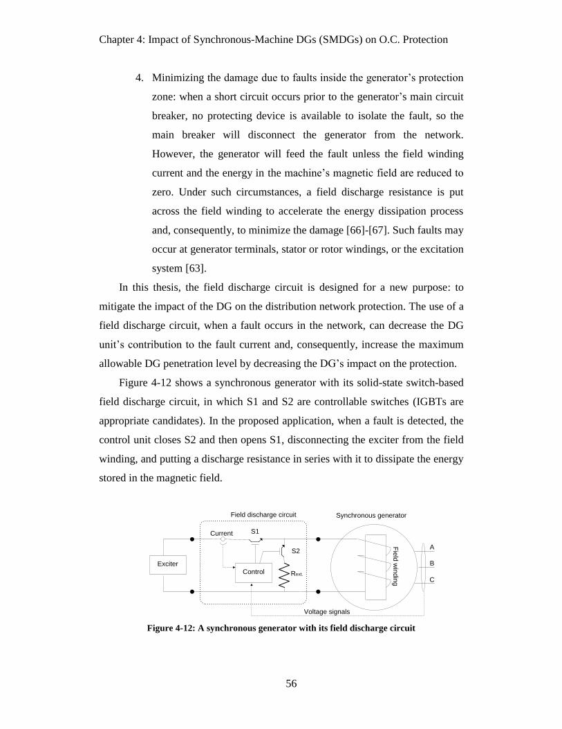
Chapter 4: Impact of Synchronous-Machine DGs (SMDGs) on O.C. Protection
56
4. Minimizing the damage due to faults inside the generator’s protection
zone: when a short circuit occurs prior to the generator’s main circuit
breaker, no protecting device is available to isolate the fault, so the
main breaker will disconnect the generator from the network.
However, the generator will feed the fault unless the field winding
current and the energy in the machine’s magnetic field are reduced to
zero. Under such circumstances, a field discharge resistance is put
across the field winding to accelerate the energy dissipation process
and, consequently, to minimize the damage [66]-[67]. Such faults may
occur at generator terminals, stator or rotor windings, or the excitation
system [63].
In this thesis, the field discharge circuit is designed for a new purpose: to
mitigate the impact of the DG on the distribution network protection. The use of a
field discharge circuit, when a fault occurs in the network, can decrease the DG
unit’s contribution to the fault current and, consequently, increase the maximum
allowable DG penetration level by decreasing the DG’s impact on the protection.
Figure 4-12 shows a synchronous generator with its solid-state switch-based
field discharge circuit, in which S1 and S2 are controllable switches (IGBTs are
appropriate candidates). In the proposed application, when a fault is detected, the
control unit closes S2 and then opens S1, disconnecting the exciter from the field
winding, and putting a discharge resistance in series with it to dissipate the energy
stored in the magnetic field.
Control
Exciter
S1
S2
Rext.
Field discharge circuit
Voltage signals
Current
Fie
ld w
ind
ing
Synchronous generator
A
B
C
Figure 4-12: A synchronous generator with its field discharge circuit

Chapter 4: Impact of Synchronous-Machine DGs (SMDGs) on O.C. Protection
57
In order to investigate the effectiveness of this idea, the distribution network
shown is Figure 4-13 was simulated in Matlab/SIMULINK. In this system,
embedding the DG at any of points S, A or B may cause miscoordination between
B1 and B2. In this simulation, the SMDG was arbitrarily embedded at S. The
synchronous machine’s parameters were collected from [51] and tabulated in
Table 4-5.
S
DG
Net. B1 B2
FL1 L2 L3 L4
A B C D
T
Figure 4-13: A sample distribution network with synchronous-machine DG
Figure 4-14 shows the RMS of the generator’s output current during the fault and
Figure 4-15 shows the RMS of its ac component. Note that most protection
devices such as the O.C. relays filter the dc component of the fault current and
operate based on the RMS of the ac component. On the other hand, some other
devices such as fuses operate based on the RMS of total current. The factor k
shows the ratio of the total field circuit’s resistance, when the field discharge is
applied, to its original resistance ( ( . ) /ext f fk R R R ).
Figure 4-14: RMS of machine’s output current during 3-phase fault at point F
0.04 0.08 0.12 0.16 0.21
2
3
4
5
6
7
8
time (s)
I RM
S(p
.u.)
Traditional exc.
Field discharge (K=3.7)
Field discharge (K=6.25)
Field discharge (K=15)

Chapter 4: Impact of Synchronous-Machine DGs (SMDGs) on O.C. Protection
58
Figure 4-15: RMS ac component of machine’s output current during 3-phase fault at point F
As Figure 4-15 reveals, except for the synchronous-machine DG with
traditional excitation, the ac components of the machine’s output currents are
decreasing. This figure also shows that applying the field discharge can
remarkably decrease the ac component of the synchronous machine’s output
during the fault. In the studied case, the value of this current .2 sec. after the
beginning of the fault is 1.53, 1.25 and 0.64 per-unit for k=3.7, 6.25 and 15,
respectively.
In addition, simulation results showed that utilizing the field discharge circuit
could decrease machine’s contribution to single phase faults as well as
symmetrical faults. Figure 4-16 shows the RMS of the generator’s output current
at phase a during the phase a-to-ground fault and Figure 4-17 shows the RMS of
its ac component. As these figures reveal, field discharge circuit can restrict the
machine’s contribution to single phase faults.
Figure 4-16: RMS of machine’s output current during 1-phase fault at point F
0.04 0.08 0.12 0.16 0.20
1
2
3
4
5
6
7
time (s)
Iac
RM
S(p
.u.)
Traditional exc.
Field discharge (k=3.7)
Field discharge (k=6.25)
Field discharge (k=15)
0 0.04 0.08 0.12 0.16 0.21
1.5
2
2.5
3
3.5
time (s)
I RM
S(p
.u.)
Traditional exc.
Field discharge (K=3.7)
Field discharge (K=6.25)
Field discharge (K=15)

Chapter 4: Impact of Synchronous-Machine DGs (SMDGs) on O.C. Protection
59
Figure 4-17: RMS ac component of machine’s output current during 1-phase fault at point F
In addition, from these figures it can be concluded that larger resistances lead
to faster decay in the ac component. However, the field discharge resistance
causes overvoltage on the field winding (see Figure 4-18). This overvoltage must
not be higher than the winding’s maximum permissible voltage. In the next
sections it will be shown that k=3.7 is the largest resistance that can be used for a
DG with 220V field’s rated voltage, and that k=6.25 is the largest resistance for a
DG with 110V field’s rated voltage. Therefore, k=15 is not practical and is just
used only to clearly demonstrate the impact of the field discharge resistance.
Figure 4-18: Voltage which appears at the field winding during the fault
4.5 Detailed analysis
In this sub-section, the time constants and operational reactances of a
synchronous machine are reviewed, and the effect of the field discharge
application on these parameters and, consequently, on the machine’s fault current
is analyzed.
Note: Although in practical condition, it is more realistic to consider the
generator’s input power constant during the fault, in the calculations and
simulations in this section, the synchronous generator’s speed is assumed to be
0 0.04 0.08 0.12 0.16 0.20
0.5
1
1.5
2
2.5
3
3.5
time (s)
Iac
RM
S(p
.u.)
Traditional exc.
Field discharge (K=3.7)
Field discharge (K=6.25)
Field discharge (K=15)
0.04 0.08 0.12 0.16 0.20
10
20
30
40
time (s)
Ab
so
lute
va
lue
of
Fie
ld v
olta
ge
(p
.u.)
k=3.7
k=6.25
k=15

Chapter 4: Impact of Synchronous-Machine DGs (SMDGs) on O.C. Protection
60
constant, so that the equations can be solved mathematically. This assumption
does not have significant effect on the resultant short circuit current and the
conclusion about the effect of field discharge circuit on it.
In 4.1, it was shown that the d-axis flux linkage of a synchronous machine
can be written in terms of the d-axis current and the machine’s excitation voltage
as follos [49]:
0 0
( ) ( )dd d F
x p G pi u
(4-17)
For detailed analysis, and are written as follows:
2
4 5 4 6
02
1 2 1 3
1
1d d
T T p T T px p L
T T p TT p
(4-18)
0
2
1 2 1 3
1
1
kd md
F
T p LG p
T T p TT p R
(4-19)
where
1
0
1( )md F
F
T X XR
(4-20)
2
0
1( )md kd
kd
T X XR
(4-21)
3
0
1( )md F
kd
kd md F
X XT X
R X X
(4-22)
4
0
1( )md a
F
F md a
X XT X
R X X
(4-23)
5
0
1( )md a
kd
kd md a
X XT X
R X X
(4-24)
6
0
1( )md a F
kd
kd md a md F F a
X X XT X
R X X X X X X
(4-25)
0
kdkd
kd
XT
R
(4-26)
In order to obtain the principal time constants of the machine, the operational
impedance Xd (p) should be re-written as (4-2). Then

Chapter 4: Impact of Synchronous-Machine DGs (SMDGs) on O.C. Protection
61
' " 2
0 0 1 2 1 3(1 )(1 ) 1d dT p T p T T p TT p (4-27)
' " 2
4 5 4 6(1 )(1 ) 1d dT p T p T T p T T p
(4-28)
By solving (4-27) and (4-28), the principal time constants of d-axis will be
obtained. However, as normally Rkd≫RF, following approximations have been
accepted in references [60]:
'
4dT T (4-29)
"
6dT T
(4-30)
'
0 1dT T
(4-31)
"
0 3dT T
(4-32)
Similarly, Xq (p) is defined as follows:
"
"
0
(1 )( )
(1 )
q
q q
q
T px p X
T p
(4-33)
where
"
0
1( )
mq a
q kq
kq mq a
X XT X
R X X
(4-34)
"
0
0
1( )q mq kq
kq
T X XR
(4-35)
During the sub-transient condition, the operational impedances are as follows:
' ""
' "
0 0
lim ( ) d dd p d d
d d
T TX x p X
T T (4-36)
"
"
"
0
lim ( )q
q p q q
q
TX x p X
T
(4-37)
During the transient condition, when the damper windings have no effect, the
operational impedance is as follows:
''
'
0
dd d
d
TX X
T (4-38)

Chapter 4: Impact of Synchronous-Machine DGs (SMDGs) on O.C. Protection
62
Finally, during the steady state operation of a synchronous machine, the
operational impedances are Xd (p=0) and Xq (p=0), which are Xd and Xq,
respectively.
Now that the operational reactances and time constants of synchronous machine
have been reviewed, the effect of the field discharge on these parameters and,
consequently, on the machine’s fault current can be determined. In the field
discharge application, when a fault is detected, the control unit closes S2 and then
opens S1. Because the operation time of control unit and switches is much less
than the machine’s time constants, the field discharge activation is considered to
be instantaneous in this thesis. In addition, the field discharge operation can be
considered as combining two actions together: (a) removing excitation and (b)
increasing the field circuit’s resistance. In the following paragraphs, the effects of
each of these actions on generator’s short circuit current are studied separately,
and then, the effect of the field discharge circuit operation is obtained as the
superposition of these effects.
The effect of excitation removal is disappearing (4-14) (the steady-state part of
the ac component, which is caused by the excitation voltage) from the generator’s
fault current. Figure 4-19 shows the short circuit current of a synchronous
generator, and Table 4-5 lists its parameters, when the field winding was short-
circuited (field discharge with zero external discharge resistance). As Figure 4-19
(a) reveals, the steady state value of current is zero. Figure 4-19 (b) shows the first
18 cycles of Figure 4-19 (a).
(a)
(b)
Figure 4-19: Synchronous generator’s fault current with short circuited field winding, (a)
Complete waveform, (b) first 18 cycles
0 0.5 1 1.5 2 2.5 3 3.5 4 4.5-6
-4
-2
0
2
4
6
time (s)
Curr
ent
(p.u
.)
0 0.05 0.1 0.15 0.2 0.25 0.3
-4
-2
0
2
4
6
time (s)
Curr
ent
(p.u
.)
Simulated
Calculated

Chapter 4: Impact of Synchronous-Machine DGs (SMDGs) on O.C. Protection
63
To take the effect of the field discharge resistance into account, RF should be
replaced with RF+Rext. in calculating T1 and T4 and, consequently, also T’d0 and
T’d where Rext. is the field discharge resistance. As a result, when the discharge
resistance (Rext=(k-1)RF) is added in series to the field winding at the fault
instance, the following changes in the machine’s time constants are anticipated:
''
,
0
1 md a dd new F
F md a
X X TT X
kR X X k
(4-39)
'
' 00,
0
1 dd new md F
F
TT X X
kR k
(4-40)
Moreover, if (4-39) and (4-40) are substituted into (4-36) and (4-38), the
operational reactances are not expected to be changed when a discharge resistance
is put in series with the field winding. As a result, the generator’s output current is
expected to be achieved by substituting T’d and T’d0 with T’d/k and T’d0/k in (4-9),
respectively. Figure 4-20 shows the generator’s output current when a discharge
resistance is added to the field circuit at the fault instant.
(a) (b)
Figure 4-20: Synchronous generator’s fault current with discharge resistance in series with field
winding, (a) Complete waveform, (b) first 6 cycles
If Figure 4-20 (a) is compared with Figure 4-19 (a) it will be obvious that the
transition to the steady state in Figure 4-20 is much faster than that in Figure 4-19.
As well, Figure 4-20 (b) shows that (4-39) and (4-40) are not accurate enough;
i.e., the anticipated time constants are smaller than the real values, and as a result,
the expected current is not close enough to the generator’s output current because
(4-29) to (4-32) are true on the condition that Rkd≫RF. However, when a large
discharge resistance is added (k≥3), this assumption is no longer true. Under such
0 .5 1 1.5 2 2.5 3 3.5 4 4.5-4
-2
0
2
4
6
time (s)
Cu
rre
nt
(p.u
.)
0.04 .08-4
-2
0
2
4
6
time (s)
Cu
rre
nt
(p.u
.)
Simulated
Expected

Chapter 4: Impact of Synchronous-Machine DGs (SMDGs) on O.C. Protection
64
circumstances, the machine’s operational parameters should be recalculated as
follows:
11,
0
1new md F
F
TT X X
kR k (4-41)
44,
0
1 md anew F
F md a
X X TT X
kR X X k
(4-42)
Next, T’d,new and T’d0,new can be obtained by accurately solving the following
quadratic equations
' " 2
0, 0 1, 2 1, 3(1 )(1 ) 1d new d new newT p T p T T p T T p (4-43)
' " 2
, 4, 5 4, 6(1 )(1 ) 1d new d new newT p T p T T p T T p
(4-44)
and consequently, the operational reactances can be obtained as follows:
'
,'
, '
0,
d new
d new d
d new
TX X
T (4-45)
' "
,"
, ' "
0, 0
d new d
d new d
d new d
T TX X
T T
(4-46)
Figure 4-21 shows how this procedure improves the estimation of the generator’s
fault current.
Figure 4-21: Accurate estimation of the synchronous generator’s fault current with a
discharge resistance in series with its field
The effect of the field discharge circuit operation is the superposition of the
effect of these two above-mentioned actions; i.e., the generator’s current has no
steady-state part, and T’d, T’d0,, X’d and X”d are replaced by T’d,new and T’d0,new,
X’d,new and X”d,new, which are obtained from (4-41) to (4-46). Briefly, the
0 0.04 0.08
-4
-2
0
2
4
6
time (s)
Cu
rre
nt
(p.u
.)
Simulated
Expected

Chapter 4: Impact of Synchronous-Machine DGs (SMDGs) on O.C. Protection
65
generator’s output current for a three-phase solid fault at its terminals when the
field discharge circuit operates at the fault instance can be obtained as follows:
' ",
"
0 0' " '
, , ,
0" "
,
0 0" "
,
0 0"
1 1 1( )
1 1cos
2
1 1cos(2 )
2
1 1( )
d new d
a
a
q
t t
T T
a mq
d new d new d new
t
mq T
d new q
t
mq T
d new q
t
T
md
q q
i U e e cos tX X X
Ue
X X
Ue t
X X
U e sin tX X
0" "
,
0 0" "
,
1 1sin
2
1 1sin(2 )
2
a
a
t
Tmd
d new q
t
Tmd
d new q
Ue
X X
Ue t
X X
(4-47)
Figure 4-22 shows the effect of the field discharge circuit operation on the
generator’s output current during the three-phase solid fault at the generator’s
terminals. By comparing this figure with Figure 4-19, it can be concluded that the
field discharge circuit has almost no impact on the sub-transient part of the ac
component of the generator’s current (first few cycles) because the damper
windings and not the field winding play the dominant role during the sub-transient
period. In contrast, it accelerates the decrease in the transient component. Also, by
comparing this figure with Figure 4-20, it can be concluded that the field
discharge circuit removes the steady-state part of the fault current.

Chapter 4: Impact of Synchronous-Machine DGs (SMDGs) on O.C. Protection
66
(a)
(b)
Figure 4-22: Synchronous generator’s fault current with field discharge operation, (a)
Complete waveform, (b) first 9 cycles
For O.C. relay coordination, the DC part of generator’s current can be
neglected because these relays operate based on the RMS of the ac component of
current. Also, the second-order harmonic has a negligible amount. Therefore:
' ",
"
, 0 0' " '
, , ,
0 0"
1 1 1( )
1( )
d new d
q
t t
T T
a ac mq
d new d new d new
t
T
md
q
i U e e cos tX X X
U e sin tX
(4-48)
Note that θ0 is a random variable and depends on the fault instance. Since O.C.
relays operate based on the RMS of the ac component of the current, it is
advantageous to obtain the RMS of (4-48), which is as follows:
2 2
, ( )a acI t A B (4-49)
where
' ",
' " '
, , ,
1 1 1d new d
t t
T T
mq
d new d new d new
A U e eX X X
(4-50)
and
"
"
1q
t
T
md
q
B U eX
(4-51)
The operation of O.C. devices normally coincides with the generator’s transient
response. Consequently, (4-49) can be simplified by neglecting the sub-transient
.5 1 1.5 2
-4
-2
0
2
4
6
time (s)
Curr
ent
(p.u
.)
0.05 0.1 -6
-4
-2
0
2
4
6
time (s)
Curr
ent
(p.u
.)
Simulated
Calculated

Chapter 4: Impact of Synchronous-Machine DGs (SMDGs) on O.C. Protection
67
terms in (4-50) and (4-51). Such an estimation is accurate from the 4th cycle after
the fault instance (t=.05 sec.).
',
, '
,
1( ) d new
t
T
a ac mq
d new
I t U eX
(4-52)
For distant faults, assume that the equivalent impedance from the generator’s
terminals to fault is
fault fault faultZ R jX (4-53)
In this situation, the generator’s contribution can be estimated by making the
following modifications:
1. In the calculation of all time constants and operational reactances, Xa
should be replaced by Xa+Xfault.
2. In the calculation of all the time constants and operational reactances,
Rs should be replaced by Rs+Rfault.
As an example, Figure 4-24 shows the RMS ac component of the generator’s
current, when the fault happens 1.6 km away from the generator’s terminals in the
sample network shown in Figure 4-23, and the field discharge is applied (k=3).
The estimated curve is obtained from (4-52) by making the modifications
mentioned above.
DG
F
5MVA
6MVA
Z=4%
Z=.4Ω/km
1.6 km
Figure 4-23: A sample distribution feeder with SMDG
Figure 4-24: RMS ac component of generator’s fault current with field discharge operation
.1 .3 .5 .7 .9 1.1 1.3 1.5 1.7 1.90
0.5
1
1.5
2
2.5
3
time (s)
RM
S a
c c
om
po
ne
nt
of
cu
rre
nt
(p.u
.)
Simulated
Estimated

Chapter 4: Impact of Synchronous-Machine DGs (SMDGs) on O.C. Protection
68
The effect of the field discharge in reducing the generator’s RMS ac current
can now be evaluated by deducting the RMS of the ac component of (4-9) from
(4-52). As a result, the reduction in the RMS ac component of the current due to
the field discharge can be expressed as follows:
'',
' '
,
1 1 1 1[ ]d newd
tt
TT
mq
d d d d new
I t U e eX X X X
(4-54)
Figure 4-25 shows the reduction in the RMS ac component of generator
caused by the field discharge (k=3). The solid curve was obtained from simulation
and the dashed curve was obtained from (4-54). As Figure 4-25 reveals, after
t=.05 sec. (3 cycles after the fault instance), the estimated result matches the
simulated one.
Figure 4-25: Reduction in synchronous generator’s RMS ac component of fault current due
to applying field discharge
Now, by utilizing (4-54), the effect of the different values of the field
discharge resistances in reducing the generator’s fault current can be compared.
Figure 4-26 shows the reduction in the RMS ac component of the generator’s fault
current for different values of k. To explain the effect of the field discharge
operation on the protection devices’ coordination, this figure is divided into three
areas. Typically, instantaneous O.C. devices operate in area 1, extremely inverse-
time and short time-delay O.C. devices operate in area 2, and inverse and very
inverse time O.C. devices operate in area 3 [21],[68]. As this figure reveals, the
maximum reduction in the generator’s contribution due to the field discharge
operation is 0.15 p.u in area 1. This result means that means that the field
discharge is not as effective in preventing miscoordination when instantaneous
devices are involved. In area 2, maximum reduction is .8 p.u. This result means
.1 .2 .3 .4 .5-0.2
0
0.2
0.4
0.6
0.8
1
1.2
time (s)
Decre
ase in R
MS
ac c
om
ponent (p
.u.)
Simulated
Estimated

Chapter 4: Impact of Synchronous-Machine DGs (SMDGs) on O.C. Protection
69
that the field discharge can be an effective mechanism for preventing
miscoordination when extremely inverse-time and short time-delay O.C. devices
are involved. Finally, in area 3, the maximum reduction in the generator’s
contribution could be up to 1.4 p.u. This result means that field discharge is a very
effective mechanism when inverse and very inverse time O.C. devices are
involved.
3
3
2
1
Figure 4-26: Reduction in generator’s RMS ac component of fault current for different
values of field discharge resistance
The above analysis was based on the assumption that the O.C. relays
measure only the ac component of the current. However, fuses and some old
electromechanical relays operate based on the total current. In such cases, the total
RMS current of the synchronous generator should be considered. For phase a, this
current can be obtained as follows:
2 2
, ,( ) ( )a a ac a dcI I t I t (4-55)
where
, 0 0" " " "
1 1 1 1( ) cos sin
2 2a a
t t
mq T Tmda dc
d q d q
U UI t e e
X X X X
(4-56)
and
' "
"
, 0 0' " '
0 0"
1 1 1 1 1( )
1 1 1( )
( ) d d
q
t t
T T
a ac mq
d d d d d
t
T
md
q q q
i U e e cos tX X X X X
U e sin tX X
t
X
(4-57)

Chapter 4: Impact of Synchronous-Machine DGs (SMDGs) on O.C. Protection
70
According to (4-56), the dc component decays with armature’s time constant, and
is not a function of field circuit parameters. Therefore, the field discharge has no
impact on the dc component (Ia,dc). However, the field discharge can minimize Ia
by reducing the ac component of the DG’s current (Ia,ac). Figure 4-27 shows the
impact of the field discharge application on the DG’s fault current components.
As Figure 4-27 (a) reveals, when the traditional excitation system is applied,
during the transient period the dc component decreases, while the ac component
increases due to the excitation’s response to the voltage drop. This response
results in an almost constant total RMS current around 3 p.u. In contrast, as Figure
4-27 (b) reveals, when the field discharge is applied, both the ac and dc
components are decaying. This response results in a decaying total RMS current,
which decreases to around 1.4 p.u. in .2 sec. Therefore, when the field discharge
is applied, the generator makes a smaller contribution to the total fault current,
and a higher DG capacity can be embedded without causing any miscoordination,
in contrast to the cases in which the DG utilizes the traditional excitation control
during the fault.
(a)
(b)
Figure 4-27: Fault current components of synchronous generator, (a) When traditional
excitation is applied, (b) when field discharge is applied
4.6 Field discharge circuit design procedure
As Figure 4-12 reveals, the field discharge circuit is composed of 4
components: discharge resistance, two solid-state switches and a control unit
which detects the fault and triggers the circuit. In this section, the maximum
allowable field discharge resistance is obtained, and the voltage and current
ratings of the switches are determined. Next, a grid fault indicator signal is
0 .05 .1 .15 .2
0
1
2
3
4
5
time (s)
Curr
ent
(p.u
.)
dc component
ac component
Total
0 .05 .1 .15 .2
0
1
2
3
4
5
6
time(s)
Curr
ent
(p.u
.)
dc component
ac component
Total

Chapter 4: Impact of Synchronous-Machine DGs (SMDGs) on O.C. Protection
71
introduced which is monitored by control unit to detect the fault and trigger the
circuit. For the sake of simplification and due to the very fast operation of solid-
state switches, the total field discharge circuit activation process is considered in
the design procedure to be instantaneous. Finally, some correction factors are
applied to insure the reliability of the designed circuit.
4.6.1 Field discharge resistance
The first step in the design procedure is to determine the discharge resistance.
Previously in this chapter, it was shown that a larger discharge resistance leads to
a smaller d-axis transient and sub-transient time constants and that, consequently,
to a faster decay in generator’s output current. In other words, a larger resistance
can decrease the machine’s contribution to the fault current more quickly than a
smaller resistance. However, the discharge resistance causes transient overvoltage
across the field winding which is a restricting factor in the selection of the
resistance. In the following paragraphs, the field winding’s transient current and
voltage during the operation of field discharge circuit are obtained, and the
maximum allowable field discharge resistance is determined.
The maximum current flows through the field winding when a three-phase
solid fault occurs at the machine’s terminals. In such condition, when no
discharge circuit is applied to the rotor, the field’s excessive current due to the
fault can be obtained from the following equation [60]:
' "
0 0
(1 )
(1 )(1 )
md kdf
f d d
L p T pi id
R T p T p
(4-58)
where id is as (4-59). As a result, if (t) can be expressed as (4-60) [60].
' "
0' " ' "
0"
1 1 1 1 1 1cos( )
1sin( )
d d a
a
t t t
T T T
d md
d d d d d d
t
T
mq
q
i t U e e e tX X X X X X
U e tX
(4-59)
and

Chapter 4: Impact of Synchronous-Machine DGs (SMDGs) on O.C. Protection
72
' "
' '
0' " ' "0 0 ( ) 1 ( ) cos( )d d a
t t t
T T Td d kd d d kdf f f
d d d d
X X T X X Ti t i i e e e t
X T X T
(4-60)
Now, for the case with field discharge operation, (4-60) is modified by replacing
X’d and T’d with X’d,new and T’d,new (calculations described in 4.5) and decaying
the steady-state part of if to zero. Then if (t) after the field discharge activation can
be expressed as follows:
' ",
' '
, ,
, . 0' " ' "
, ,
0 2 ( ) 1 ( ) cos( )d new d a
t t t
T d d new d d newT Tkd kdf dis f
d new d d new d
X X X XT Ti t i e e e t
X T X T
(4-61)
Figure 4-28 shows the real and approximation of a generator’s field current for
k=4.
Figure 4-28: Synchronous generator’s field current during the three-phase fault at its
terminals, with field discharge circuit operation
Since Rext. =(k-1)RF, Figure 4-29 shows the rotor circuit during the discharge
operation. According to this figure, the field winding’s voltage in discharge period
can be obtained from (4-62), and its maximum value can be obtained from (4-63):
. , . , .( 1)f ext f dis f f disv t R i t k R i t (4-62)
, ,( 1)f max f f MaxV k R i
(4-63)
where if,Max is the maximum field current, which occurs either at t=.025 or
t=.0417 sec. (the second or third peak of oscillation depending on the k).
Therefore, to find if,Max, t is first replaced by .025 in (4-61), and then replaced by
.0417, and from the two obtained currents, the maximum value is selected as if,Max.

Chapter 4: Impact of Synchronous-Machine DGs (SMDGs) on O.C. Protection
73
SMRext.=(k-1)Rf
If(t)
Vf
Figure 4-29: Rotor’s circuit during field discharge circuit operation
Now, k should be restricted so that Vf,max remains lower than the winding’s
permissible insulation stress [59]. In other words, k should satisfy the following
inequality:
.
,
1per
f f Max
Vk
CR i (4-64)
where Vper. is the winding’s permissible insulation stress (equal to the standard
machine’s field dielectric test), and C=1.1 is a safety factor.
Note that if,Max itself depends on k. Consequently, in order to determine the
maximum allowable discharge resistance, the field’s maximum transient voltage
is plotted for different values of k by using (4-63). The standard manufacturing
machine field dielectric test voltage divided by C on this plot shows the maximum
allowable k.
4.6.2 Current and voltage ratings of solid state switches
Now that the field’s transient current during the fault has been obtained, the
current rating of the switches can be determined. Switch S1 is in series with
exciter. As a result, the maximum current which can flow through this switch is
equal to the exciter’s ceiling current. Switch S2 is in series with the field during
the discharge operation. Consequently, the maximum current which flows through
this switch is equal to the maximum field current which is if,Max.
When S1 is off, the voltage across it is equal to the field winding’s voltage.
As a result, rated voltage of S1 should be equal or greater than the standard
manufacturing machine’s field dielectric test available in [59]. When switch S2 is
off, it is in parallel with the exciter. Consequently, the maximum voltage that can
Chapter 4: Impact of Synchronous-Machine DGs (SMDGs) on O.C. Protection
74
appear across this switch is equal to the exciter’s ceiling voltage. Table 4-8
summarizes the switches’ ratings.
Table 4-8: Field discharge switches’ ratings
Vrated Irated
S1 standard machine field dielectric test Exciter’s ceiling current
S2 Exciter’s ceiling voltage if,Max
4.6.3 Grid fault detection
In the above sections, it was supposed that some mechanism accurately and
quickly detects the fault occurrence in the network and triggers the field discharge
circuit. In following, this mechanism will be described.
The first and the most important step for the trigger mechanism is fault
detection. To detect a fault, one of the generator’s local voltage or current signals
should be selected and monitored. To be an appropriate grid fault indicator, this
signal should have the following properties:
1. Its variation due to the grid faults should be so fast that the fault
occurrence is detected as quickly as possible,
2. This signal should have distinctive levels for different grid
disturbances so that close grid faults can be distinguished from other
disturbances.
Given these necessary properties, the derivative of the field’s current is an
appropriate indicative signal. For a 3-phase solid fault at the terminals, this signal
can be mathematically obtained from (4-61).
Figure 4-30 shows the derivative of the field’s current for a typical generator,
whose parameters tabulated in Table 4-5, for three different disturbances: 3-phase
fault in the generator’s neighbourhood, 1-phase fault at one of generator’s
terminals, and a large sudden load change at generator’s node. As this figure
reveals, these signals have three distinct levels in the first cycle after the
disturbances. As a result, by appropriately defining thresholds, the type of
disturbance can be easily and accurately determined. In addition, it can be seen
that for 3-phase faults in which the DG unit has the most contribution and also the

Chapter 4: Impact of Synchronous-Machine DGs (SMDGs) on O.C. Protection
75
most probable impact on the coordination, the indicative signal has an almost
instantaneous jump, which helps to detect the fault in a few milliseconds.
Figure 4-30: Field’s current derivative for three different grid disturbances
When this method is implemented, the generator’s O.C. protection is set so
that it protects the generator from damages due to overcurrent/overload. In other
words, when the field discharge circuit is implemented, the DG’s overcurrent
relay is set similarly to relays of the generators connected to the transmission
system, and there is no conflict between generator’s O.C. protection and the field
discharge application. The IEEE Std. C.37.102-2006 can be followed in this
case [25].
The last step is detecting the fault clearance and disabling the field discharge
circuit, which can be detected by monitoring the generator’s terminal voltages.
4.7 Mitigation of SMDG’s impact on coordination: case studies
This section presents three case studies. The first case illustrates the field
discharge circuit design procedure, the second one focuses on the impact of the
field discharge circuit in mitigating the main and back-up relays miscoordination,
and the last one shows the ability of field discharge circuit to re-gain the fuse-
recloser coordination.
4.7.1 Case I: Field discharge circuit design
In this sub-section, a field discharge circuit is designed for the generator
whose parameters are tabulated in Table 4-5. The first step is to determine the
field discharge resistance. As it was mentioned in the previous section, in order to
determine the maximum allowable discharge resistance, the field’s maximum
transient voltage with respect to k is plotted by using (4-63). The cross of the
0 0.02 0.04-40
0
40
80
120
time (s)
dI f /
dt
3-phase fault in the network
1-phase fault at terminal
Sudden load change

Chapter 4: Impact of Synchronous-Machine DGs (SMDGs) on O.C. Protection
76
standard manufacturing machine field dielectric test voltage with this plot shows
the maximum allowable k.
According to [69], the standard field’s dielectric test for both 110V and 220V
windings, which are options for use in DGs, is 2500V. Figure 4-31 shows the
generator’s field winding’s maximum transient voltage for different values of k.
For C=1.1, the maximum allowable voltage for 110V and 220V windings is
2200V (20 and 10 p.u., respectively). These voltages occur at k=6.25 and k=3.7,
respectively. If the field winding’s rated voltage is 220V, then maximum k is 3.7,
and as a result, Rext.=(3.7-1) Rf=2.7Rf.
Figure 4-31: Field winding’s maximum voltage due to discharge circuit operation
The second step is to determine the solid-state switches ratings. To do so,
if,Max should be determined, which is equal to the current rating of S2. From
(4-61), if,Max =1.56 if(0), where if(0) is the excitation current during the generator’s
full-load steady-state operation. For a typical generator smaller than 30MW, if(0)
could be in the range of 15A. Then, if,Max =1.56*15=23.4A.
In addition to if,Max, the exciter’s ceiling voltage and current should be
obtained from the exciter’s data sheet. For a typical SIEMENS SIPOL [70],
ceiling current is 20A, which is equal to the rated current of S1, and the ceiling
voltage is 1.6 times the rated voltage; i.e., 1.6*220=352V, which is equal to the
rated voltage of S2. All the switches’ ratings are summarized in Table 4-9.
Table 4-9: Switches’ ratings in the studied case
Vrated Irated
S1 2500 V 20 A
S2 352 V 23.4 A

Chapter 4: Impact of Synchronous-Machine DGs (SMDGs) on O.C. Protection
77
The last step is to design the trigger mechanism. As was mentioned in 5.3, the
derivative of field current is an appropriate grid fault indicator. Suppose that the
field discharge circuit is desired to operate only if 3-phase faults occur at the
distribution system. In this case, the threshold is set to 60p.u./sec. As Figure 4-32
shows, single-phase faults and sudden load changes cannot cause the signal to
reach this level. In contrast, the 3-phase faults exceed this level in a few ms.
Therefore, the control circuit monitors the indicator signal and triggers the
discharge circuit when the signal exceeds the threshold of 60p.u./sec.
4.7.2 Case II: main and back-up relays coordination
Consider the sample system studied in sub-section 4.3.1 again. It was shown
that when a SMDG unit (with its parameters tabulated in Table 4-5) is added in
the substation, its contribution to fault increases the fault current which flows
through protection devices, and such increase causes miscoordination between B1
and B2 for DGs with higher capacities than 5MW (see Figure 4-6 and Figure 4-7).
Nevertheless, field discharge circuit operation can maintain coordination
between B1 and B2 for DG units larger than 5MW. Imagine that the field’s rated
voltage is 220V. According to previous sub-section, maximum allowable k is 3.7.
Now, consider that a 6.5 MW DG is connected to the substation through a
transformer with MVA equal to 130% of DG’s, and 6% series impedance. In this
system, Figure 4-32 shows the fault current at F3. As this figure demonstrates,
when a field discharge resistance (k=3.7) is applied to the DG during the fault, it
reduces DG’s contribution, so that the fault current is decreased below 4440A in
less than .1s which blocks the operation of instantaneous relay at B1 and,
consequently, maintains the coordination. Table 4-10 shows the protection
devices’ operation times for fault at F3, and 6.5MW DG with/without field
discharge operation at substation.

Chapter 4: Impact of Synchronous-Machine DGs (SMDGs) on O.C. Protection
78
Figure 4-32: Effect of field discharge circuit on eliminating the impact of a 6.5MW SMDG
Table 4-10: The relays’ currents and operation times for fault at F3 and 6.5MW DG
IR1 TR1 IR2 TR2
Without field discharge 4504 .1 4483 .1
With field discharge 4430 .72 4413 .1
As it was shown in this case study, field discharge is able to increase
maximum allowable capacity of DG from 5MW, which is equal to 48.5% of total
load in distribution system, to 6.5MW which is equal to 63% of total load.
However, field discharge is not able to mitigate miscoordination for capacities
higher than 63%. Moreover, as Figure 4-32 demonstrates, if the operation time of
the instantaneous elements were .04sec. or less, field discharge would have no
effect in such short period, and no increase would occur in the DG’s maximum
capacity.
4.7.3 Case III: Fuse-recloser coordination
Consider the system studied in sub-section 4.3.2. It was shown that if a
synchronous-machine DG is added at bus 1, this DG contributes to the fault and
increases the current through the fuse and the recloser. For a SMDG larger than
1600 kW (see Figure 4-33), the fault current will be higher than 1475A for more
than .1s and, consequently, the fuse will melt sooner than recloser’s operation (the
DG’s parameters are the same as those in Case I). However, by utilizing the field
discharge, the DG capacity can be larger than 1600kW without losing
coordination. Figure 4-34 shows the impact of the field discharge circuit operation
on the fault current for the case with 2400kW DG. As this figure shows, when no
field discharge is applied, the fault current is higher than the coordination
0 0.05 0.1 0.15
4500
5500
6500
time (s)
Cu
rre
nt
(A)
DG with field discharge
DG with traditional control
Coordination boundary

Chapter 4: Impact of Synchronous-Machine DGs (SMDGs) on O.C. Protection
79
boundary, and the fuse melts sooner than the recloser’s operation. In contrast,
when the field discharge is applied, the fault current is reduced below the
coordination boundary in less than .1s, and as a result, the recloser operates
sooner than the fuse, and the coordination is maintained. This result means that
maximum DG capacity can be increased by 50%, from protection prospective,
without any need to modify the protection system.
Figure 4-33: Fuse and recloser fault current when a 1600kW DG is added at bus 1
Figure 4-34: Effect of field discharge circuit to eliminate the impact of a 2400kW DG on
coordination
4.8 Impact of field discharge on voltage recovery
In this section, the post-fault performance of the SMDG when using the
proposed field discharge strategy is compared with the performance of SMDG
with traditional excitation strategy. The main aim is to demonstrate the impact of
the field discharge on the voltage recovery in post-fault period.
Consider the network shown in Figure 4-13 with the SMDG operating at a
unity power factor before the fault occurrence. When a three-phase fault happens
at point F, the generator’s d-axis flux suddenly decreases, and the machine starts
absorbing the reactive power (see Figure 4-35, t=0~t=.16 Sec.). When the fault is
cleared, another abrupt change in the reactive power happens, and then the
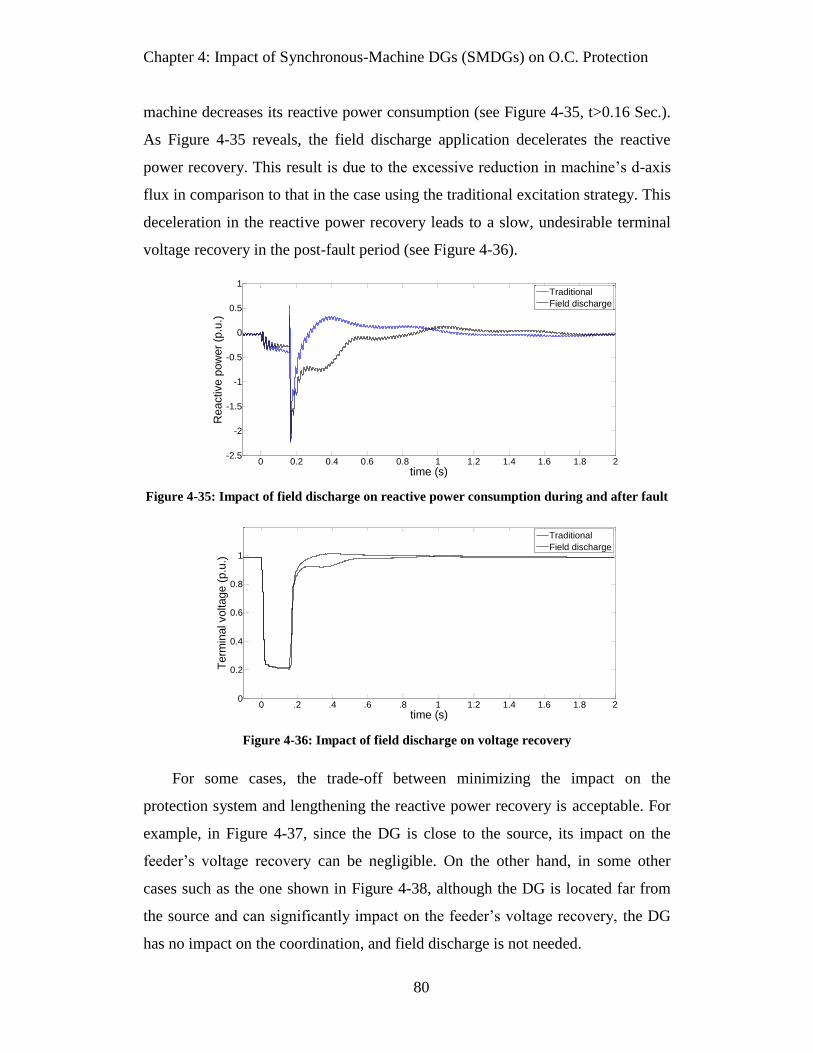
Chapter 4: Impact of Synchronous-Machine DGs (SMDGs) on O.C. Protection
80
machine decreases its reactive power consumption (see Figure 4-35, t>0.16 Sec.).
As Figure 4-35 reveals, the field discharge application decelerates the reactive
power recovery. This result is due to the excessive reduction in machine’s d-axis
flux in comparison to that in the case using the traditional excitation strategy. This
deceleration in the reactive power recovery leads to a slow, undesirable terminal
voltage recovery in the post-fault period (see Figure 4-36).
Figure 4-35: Impact of field discharge on reactive power consumption during and after fault
Figure 4-36: Impact of field discharge on voltage recovery
For some cases, the trade-off between minimizing the impact on the
protection system and lengthening the reactive power recovery is acceptable. For
example, in Figure 4-37, since the DG is close to the source, its impact on the
feeder’s voltage recovery can be negligible. On the other hand, in some other
cases such as the one shown in Figure 4-38, although the DG is located far from
the source and can significantly impact on the feeder’s voltage recovery, the DG
has no impact on the coordination, and field discharge is not needed.
0 0.2 0.4 0.6 0.8 1 1.2 1.4 1.6 1.8 2-2.5
-2
-1.5
-1
-0.5
0
0.5
1
time (s)
Reactive p
ow
er
(p.u
.)
Traditional
Field discharge
0 .2 .4 .6 .8 1 1.2 1.4 1.6 1.8 20
0.2
0.4
0.6
0.8
1
time (s)
Term
inal voltage (
p.u
.)
Traditional
Field discharge
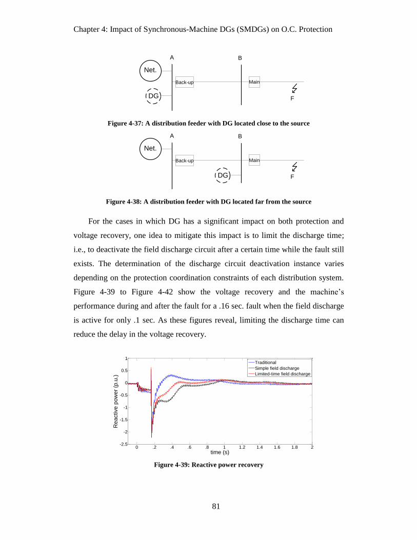
Chapter 4: Impact of Synchronous-Machine DGs (SMDGs) on O.C. Protection
81
A
Net.
Back-up Main
FDG
B
Figure 4-37: A distribution feeder with DG located close to the source
A
Net.
Back-up Main
FDG
B
Figure 4-38: A distribution feeder with DG located far from the source
For the cases in which DG has a significant impact on both protection and
voltage recovery, one idea to mitigate this impact is to limit the discharge time;
i.e., to deactivate the field discharge circuit after a certain time while the fault still
exists. The determination of the discharge circuit deactivation instance varies
depending on the protection coordination constraints of each distribution system.
Figure 4-39 to Figure 4-42 show the voltage recovery and the machine’s
performance during and after the fault for a .16 sec. fault when the field discharge
is active for only .1 sec. As these figures reveal, limiting the discharge time can
reduce the delay in the voltage recovery.
Figure 4-39: Reactive power recovery
0 .2 .4 .6 .8 1 1.2 1.4 1.6 1.8 2-2.5
-2
-1.5
-1
-0.5
0
0.5
1
time (s)
Reactive p
ow
er
(p.u
.)
Traditional
Simple field discharge
Limited-time field discharge

Chapter 4: Impact of Synchronous-Machine DGs (SMDGs) on O.C. Protection
82
Figure 4-40: Terminal voltage recovery
Figure 4-41: d-axis flux
Figure 4-42: d-axis flux
Another idea for accelerating the voltage recovery after a fault is to modify
the discharge circuit so that it can speed up the flux increase. In the previous sub-
sections, it was shown that a series resistance with the field winding decreases
machine’s transient time constant. As a result, similar to the discharging process,
a series resistance can be temporarily applied to the field circuit after the fault
0 .2 .4 .6 .8 1 1.2 1.4 1.6 1.8 20
0.2
0.4
0.6
0.8
1
time (s)
Term
inal voltage (
p.u
.)
Traditional
Simple field discharge
Limited-time field discharge
0 .2 .4 .6 .8 1 1.2 1.4 1.6 1.8 20.1
0.2
0.3
0.4
0.5
0.6
0.7
0.8
0.9
1
time (s)
d-a
xis
flu
x (
p.u
.)
Traditional
Simple field discharge
Limited-time field discharge
0 .2 .4 .6 .8 1 1.2 1.4 1.6 1.8 20
1
2
3
4
5
6
time (s)
Curr
ent (p
.u.)
Traditional
Simple field discharge
Limited-time field discharge

Chapter 4: Impact of Synchronous-Machine DGs (SMDGs) on O.C. Protection
83
clearance to accelerate the recovery process. Figure 4-43 shows the SMDG with
the modified field discharge circuit.
Control
Exciter
S1
S2
Rext.
Field discharge circuit
Voltage signals
Current F
ield
win
din
g
Synchronous generator
A
B
C
R0
S0
Figure 4-43: SMDG with modified field discharge circuit
In this circuit, during normal condition S0 and S1 are close, and S2 is open,
so the exciter is directly connected to the field circuit. During the fault, S2 is
closed, and S1 is opened to discharge the circuit. When the fault is cleared, S1 is
closed, and S2 is opened to connect the exciter. At this moment, S0 is also
opened. By this action, R0 is put in series with the field and exciter, and shortens
the machine’s transient time constant in order to accelerate building up the flux.
After a certain amount of time (T1), S0 is closed, and the circuit returns to its
normal condition.
To demonstrate the improvement acheived in the recovery process by
modifying the discharge circuit, the system shown in Figure 4-13 was simulated,
and the modified field discharge circuit was applied to the SMDG. In this study,
the fault starts at t=0 and is cleared at t=.16 Sec. Therefore, ideally, S1 is open
from t=0 to t=.16 Sec. In this period, S2 is closed to discharge the field circuit.
After t=.16 Sec. both S2 and S0 are open. Finally, S0 is closed at t=.25 sec. Also,
in this simulation, Rext=R0=6.25Rfield. As Figure 4-44 reveals, the reactive power
recovery is much faster when the modified circuit is applied. Likewise, as Figure
4-45 shows, voltage recovery is much faster in the case with a modified circuit
than in the case with a simple discharge circuit. Also, Figure 4-46 shows how the
additional resistance accelerates the building up of the flux. Figure 4-47 shows the
output current during and after the fault for each excitation method, and finally,
Figure 4-48 shows the exciter voltage (for the IEEE type 1 excitation system).

Chapter 4: Impact of Synchronous-Machine DGs (SMDGs) on O.C. Protection
84
Figure 4-44: Reactive power recovery
Figure 4-45: Terminal voltage recovery
Figure 4-46: d-axis flux
0 0.2 0.4 0.6 0.8 1 1.2 1.4 1.6 1.8 2-2.5
-2
-1.5
-1
-0.5
0
0.5
1
time (s)
Reactive p
ow
er
(p.u
.)
Traditional
Simple field discharge
Modified field discharge
0 .2 .4 .6 .8 1 1.2 1.4 1.6 1.8 20
0.2
0.4
0.6
0.8
1
time (s)
Term
inal voltage (
p.u
.)
Traditional
Simple field discharge
Modified field discharge
0 .2 .4 .6 .8 1 1.2 1.4 1.6 1.8 20.1
0.2
0.3
0.4
0.5
0.6
0.7
0.8
0.9
1
time (s)
d-x
is flu
x (
p.u
.)
Traditional
Simple field discharge
Modified field discharge
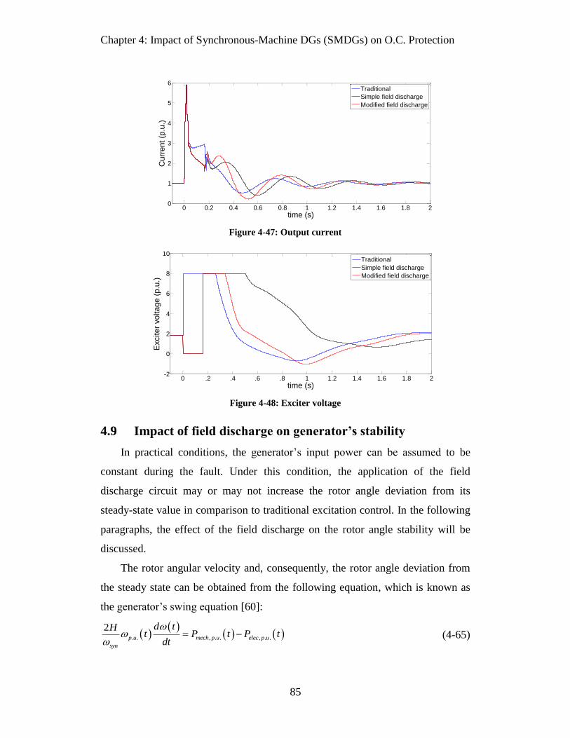
Chapter 4: Impact of Synchronous-Machine DGs (SMDGs) on O.C. Protection
85
Figure 4-47: Output current
Figure 4-48: Exciter voltage
4.9 Impact of field discharge on generator’s stability
In practical conditions, the generator’s input power can be assumed to be
constant during the fault. Under this condition, the application of the field
discharge circuit may or may not increase the rotor angle deviation from its
steady-state value in comparison to traditional excitation control. In the following
paragraphs, the effect of the field discharge on the rotor angle stability will be
discussed.
The rotor angular velocity and, consequently, the rotor angle deviation from
the steady state can be obtained from the following equation, which is known as
the generator’s swing equation [60]:
. . , . . , . .
2p u mech p u elec p u
syn
d tHt P t P t
dt
(4-65)
0 0.2 0.4 0.6 0.8 1 1.2 1.4 1.6 1.8 20
1
2
3
4
5
6
time (s)
Curr
ent (p
.u.)
Traditional
Simple field discharge
Modified field discharge
0 .2 .4 .6 .8 1 1.2 1.4 1.6 1.8 2-2
0
2
4
6
8
10
time (s)
Exciter
voltage (
p.u
.)
Traditional
Simple field discharge
Modified field discharge

Chapter 4: Impact of Synchronous-Machine DGs (SMDGs) on O.C. Protection
86
where ωp.u.(t) is the rotor’s per-unit angular speed, Pmech,p.u.(t) is the per-unit
mechanical power of the prime mover (the generator’s input power), Pelec.,p.u.(t) is
the per-unit electric output power of the generator, ωsyn is the synchronous angular
speed, and H is the inertia constant. Although for the fault cases, this equation can
be solved only numerically, it can help in interpreting the sample simulation result
and in reaching a conclusion.
For 3-phase faults near the generator, the voltages at the terminals are almost
zero. As a result, regardless of the excitation control method, the average of
Pelec,p.u.(t)≈0, and rotor angle deviations during the fault are the same for the case
with the traditional excitation control and the case with the field discharge. For
further illustration, the network shown in Figure 4-49 was simulated. This
network is a 25 kV distribution system with Zsource=(1.625+j5.5187)Ω and
Zline=(.24+j.26)Ω/km. The generator’s parameters are the same as those in the
previous section, and its inertia constant is 1.5 sec. Figure 4-50 shows the output
electric power and rotor angle deviation during and after a .1 sec. 3-phase fault at
bus 1. As figure reveals, both the output power and rotor angle deviation match
for both cases during the fault (t=0 ~ t=.1 sec.).
Substation
Net.
1 km
2 3
4
L
11.6 km
1
DG
T
1 km 1 km
Figure 4-49: Sample distribution network simulated for stability studies

Chapter 4: Impact of Synchronous-Machine DGs (SMDGs) on O.C. Protection
87
Figure 4-50: Generator’s output current and rotor angle deviation for .1 sec. 3-phase fault at
terminals
When the fault is distinguished at t=.1s., the generator in both cases generates
the electric power. However, in the field discharge case, the average of Pelec.,p.u.(t)
from t=.1s to t=.2s is lower than that in the traditional excitation case. In the field
discharge case, after the fault the machine has a lower d-axis flux linkage (see
Figure 4-51) and starts to build it up. Thus, it can produce lower synchronizing
power at the beginning of the post-fault period. Consequently, the rotor angle
deviation is higher in this case. The lower synchronizing power at the beginning
of the post-fault period slightly decreases the Critical Clearing Time (CCT) for
the fault near the terminals. For example, for a 5MW generator with H=1.5s, the
CCT for traditional excitation is 145 ms, and for the field discharge with k=6.25,
the CCT is 135ms (10ms reduction).
Figure 4-51: Generator’s d-axis flux during and after fault
For farther faults, because the voltages at the terminals are not zero,
Pelec.,p.u.(t)>0 during the fault. As a result, the CCTs are higher than those in the

Chapter 4: Impact of Synchronous-Machine DGs (SMDGs) on O.C. Protection
88
cases in which a fault occurs at the terminals. However, in the case with the field
discharge, the machine generates less electric power during the fault than the case
with traditional excitation. Consequently, rotor angle deviation during the fault is
larger in this case, and the reduction in the CCT due to applying the field
discharge is higher than when the fault occurs at the terminals. Figure 4-52 shows
the output power and rotor angle deviation of generator when a .2 sec. 3-phase
fault occurs at bus 4 (12.6 km away from the generator) of the simulated network.
In this case, the CCTs are 365ms and 245ms for the traditional excitation and the
field discharge, respectively.
Table 4-11 summarizes the CCTs for the faults at different buses in the
simulated system. As this table reveals, in theory, for the farther faults the
difference between the CCTs of the constant excitation and field discharge is
higher. However, in practice, when the fault is too far from the generator, the DG
unit barely contributes to the fault and has no impact on the coordination.
Consequently, the field discharge is not applied in such cases.
To sum up, the field discharge is applied for close faults, to which the
generator has high contribution. In such faults, the effect of the field discharge
application on the CCT is low enough to be tolerated. On the other hand, for
farther faults, the generator makes a small contribution. So, the field discharge is
not needed. Consequently, the reduction in the CCT due to the application of the
field discharge is not a concern with these faults.
Figure 4-52: Generator’s output power and rotor angle deviation for .2 sec. 3-phase fault 8.1
km away from generator

Chapter 4: Impact of Synchronous-Machine DGs (SMDGs) on O.C. Protection
89
Table 4-11: CCT for 3-phase solid fault at different busses
CCT (ms)
Traditional excitation Field discharge (k=6.25)
Bus 1 145 135
Bus 2 165 145
Bus 3 180 155
Bus 4 365 245
4.10 Conclusion
In this chapter, the contribution of SMDGs to the fault current was analyzed,
and their impact on the O.C. coordination was investigated. From both the
mathematical analysis and the simulations, the following conclusions are made:
1. During the SMDG’s sub-transient response, the machine’s fault
current is 4~8 p.u. and lasts for up to 3 cycles. The damper windings’
parameters are the dominating factors in this period.
2. During the SMDG’s transient response, the machine’s fault current is
3~5 p.u. This part of the machine’s response gradually decays with a
transient time constant in the range of 1-2 sec. Field winding’s
parameters are the dominating factors in this period. This period
coincides with the operation of the major O.C. devices in the
distribution system, and this part of the machine’s response can
significantly impact on the coordination.
3. After the transient response, the steady state response appears. The
magnitude of the current is around the rated current in this period.
4. In order to restrict the machine’s fault current contribution in the
transient period and, consequently, to mitigate the impact of the
machine on the O.C. protection coordination, the field discharge
application was proposed. This circuit disconnected the machine’s
excitation and decreased the machine’s transient time constant. As a
result, the machine’s fault current decayed faster, and no steady state
current existed.

Chapter 4: Impact of Synchronous-Machine DGs (SMDGs) on O.C. Protection
90
5. It was shown that applying the field discharge circuit sufficiently
reduced the generator’s contribution to the fault current, and as a
result, prevented miscoordination when short time-delay and/or
inverse-time O.C. relays were involved.
6. A design procedure was proposed for the field discharge circuit, and
this circuit was applied to the simulated SMDG. The case studies
showed the proposed method significantly increased the SMDG’s
compatibility with the distribution system by mitigating its impact on
the protection system’s coordination.
7. The impact of field discharge application on the post-fault voltage
recovery and also on the generator’s stability was analyzed. The
results showed that the field discharge undesirably delayed the voltage
recovery. Therefore, mitigations were proposed to address this
concern.

Chapter 5: Harmonic Analysis of DFIG-based Wind Farms
91
Chapter 5
Harmonic Analysis of DFIG-based
Wind Farms
In the previous chapters, the impact of DGs on the O.C. protection was
discussed, and mitigation methods were proposed. In this chapter, the main focus
is on the power quality impact of DGs, specifically wind energy systems. Since
the Doubly-Fed Induction Generator (DFIG) is one of the most popular generator
types used in the wind energy systems, a harmonic analysis is presented for
DFIGs during balanced steady state operation and a harmonic model is proposed
for DFIG-based wind farms which can be used instead of their detailed models in
power system harmonic studies.
The modelling methodology and its prerequisites are presented in Section 5.1.
Next, the sinusoidal Pulse-Width Modulation (PWM) switching technique for 3-
phase converters is reviewed in Section 5.2. In Section 5.3, a harmonic modelling
method is proposed for DFIG-based wind systems. Section 5.4 covers the
simulation results, which verify the modelling. Next, a method to estimate the
parameters required for calculating the average harmonic voltages and currents is
proposed in Section 5.5. Section 5.6 presents the determination of the worst-case
harmonic scenario. Next, the non-characteristic harmonics are introduced and
investigated in Section 5.7. Section 5.8 presents a comparison between the
harmonic emissions from DFIG-based wind farms and those from other harmonic
sources. The conclusions are presented in Section 5.9.

Chapter 5: Harmonic Analysis of DFIG-based Wind Farms
92
5.1 Methodology
Figure 5-1 shows a DFIG-based wind farm. In this figure, one DFIG system
is shown in detail while the other DFIG systems are shown as boxes. As this
figure reveals, each DFIG system consists of a wound-rotor induction machine
and two converters sharing a DC link. Figure 5-2 shows the equivalent circuit of
the DFIG at the fundamental frequency. In this figure, s is the slip at the
fundamental frequency and can be calculated by using (5-1).
Mechanical
torque
Rotor-side
converter
Collector
bus
Grid-side
converter
DC link
Shunt Filter
Choke
Grid
DFIG
DFIG
DFIG
Figure 5-1: DFIG-based wind farm structure
Rs Xs
Xm
X’r
vs
R’r / s
V’r / s
Figure 5-2: DFIG’s equivalent circuit at fundamental frequency
s m
s
f fs
f
(5-1)
In a DIFG system, the slip can be in the range of ±.3. In other words, the
DFIG is able to operate at both super- and sub-synchronous speeds (in the wide
operation speed range, 70~130% of the synchronous speed). In the super-
synchronous speed operation, the power is delivered through both the stator and
rotor to the network. During the sub-synchronous speed operation, the power is
delivered from the stator to the grid, while the converters inject some power (up to

Chapter 5: Harmonic Analysis of DFIG-based Wind Farms
93
30% of the stator’s power) from the grid into the rotor (see subsection 5.5.1 for
further explanation). The power injection/consumption through converters can be
up to 30% of DFIG’s rated power.
In a DFIG-based wind system, the Rotor-Side Converter (RSC) controls the
machine’s torque by injecting the appropriate voltage into the rotor at its
frequency while the Grid-Side Converter (GSC) keeps the DC link voltage
constant. In other words, if the GSC control is ideal, the dc link’s voltage is ripple
free. Consequently, the converters can be considered as two decoupled sources
shown in Figure 5-3. In Section 5.2, it is shown that each source is a periodic
PWM pulse train, which can be decomposed to a double Fourier series. Each
series includes a fundamental frequency component and harmonic components at
the odd sidebands of the converters’ switching frequencies and their multiples.
The harmonic modelling method presented in this chapter is based on the de-
coupling of the converters and decomposing each converter’s pulse train to a
Fourier series.
Mechanical torqueCollector
bus
Shunt FilterRotor-side harmonic source Grid-side harmonic source
Figure 5-3: DFIG’s equivalent circuit for harmonic analysis
Usually, the converters’ switching frequencies are higher than 1 kHz. As a
result, low-order harmonic voltages are not expected to appear at the converters’
terminals and converters are not supposed to interact with the grid at low order
harmonic frequencies. However, in the simulations these non-characteristic
components appeared. Moreover, the DC link voltage was not ripple-free. This
results cast doubt on the decoupling assumption, so, it was important to
investigate whether or not there any interaction occurred between the grid and
converters at low order harmonic frequencies. Hence, the sensitivity of
components of DC link voltage and low-order components of the voltages at the

Chapter 5: Harmonic Analysis of DFIG-based Wind Farms
94
terminals to the changes in the background harmonic voltages at the grid was
studied in a sample system (which is fully described in 5.4.1). Four scenarios
were simulated. In the first scenario, no background harmonics were present in
the grid. In the second scenario, the harmonic spectrum of the voltages measured
at a 144kV substation in the Calgary area was used as the grid’s background
harmonics (see Table 5-1). In the third scenario, the amplitude of the background
harmonics in scenario 2 was decreased by 50%. Finally, in the last scenario, the
amplitude of grid’s background harmonic voltages was 130% of those in the
second scenario.
Table 5-1: Sample spectrum for background harmonic voltages in Scenario 1
Harmonic
order Amplitude (% of rated voltage)
Angle in phase a
(degree)
5th
1.16 -258
7th
0.18 -33.7
11th
0.07 -18.2
13th
0.02 -289
Figure 5-4 shows the DC link voltage, Figure 5-5 shows its zoomed-in
version, and Figure 5-6 shows the harmonic spectrum of DC link voltage under
different scenarios. As Figure 5-6 reveals, the major components are low order (in
range of 0~1 kHz, less than that of the switching frequencies). These harmonics
are available even in the 0% background harmonic scenario. This result means
that these components are caused by the DFIG’s converters and are not from the
grid (In fact, they are non-characteristic harmonics. The source of these harmonics
is discussed in 0 5.7). Besides, Figure 5-7 reveals the changes in these
components due to the changes in the background distortion have an arbitrary
pattern.
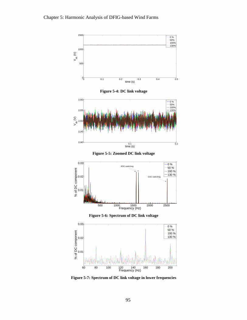
Chapter 5: Harmonic Analysis of DFIG-based Wind Farms
95
Figure 5-4: DC link voltage
Figure 5-5: Zoomed DC link voltage
Figure 5-6: Spectrum of DC link voltage
Figure 5-7: Spectrum of DC link voltage in lower frequencies
0 0.1 0.2 0.3 0.4 0.50
500
1000
1500
time (s)
Vd
c (
V)
0 %
50%
100%
130%
0.1 0.21140
1145
1150
1155
1160
time (s)
Vd
c (
V)
0 %
50%
100%
130%
500 1000 1500 2000 2500
0.01
0.02
0.03
Frequency (Hz)
% o
f D
C c
om
ponent
0 %
50 %
100 %
130 %
RSC switching
GSC switching
60 80 100 120 140 160 180 200
0.01
0.02
0.03
Frequency (Hz)
% o
f D
C c
om
ponent
0 %
50 %
100 %
130 %

Chapter 5: Harmonic Analysis of DFIG-based Wind Farms
96
Figure 5-8 shows the integer harmonics of the voltage at the GSC’s terminals
(before the choke in Figure 5-1). As this figure reveals, these components show
negligible sensitivity to the background harmonics. They were also present in the
0% background harmonic voltages scenario, and their changes were negligible in
all scenarios from the 0% scenario to the 130% scenario. In other words, no
significant interaction occurred between the converters and the grid at these
frequencies. This result means that the DC link can be decoupled and each
converter can be modeled as an independent harmonic voltage source.
Figure 5-8: Integer harmonics of GSC’s terminal voltage
5.2 Sinusoidal PWM switching technique
The majority of DFIGs utilize the sinusoidal PWM switching technique for
both RSC and GSC. Since the switching technique of converters is a key factor in
the harmonic emissions of a wind system, sinusoidal PMW switching for a 3-
phase converter is reviewed in the following paragraphs.
Figure 5-9 shows a 3-phase converter, and Figure 5-10 shows its modulation
signals. For each phase, when the reference signal is higher than that of the carrier
(vref>vcr), the upper switch in Figure 5-9 is on (S1, S3 or S5). Otherwise, the
lower switch is on (S6, S4 or S2). Figure 5-11 shows the state of S1 in one cycle.
In addition, as Figure 5-10 shows, the reference signals are displaced by 120o.
This displacement results in balanced phase-to-phase waveforms at the terminals
(see Figure 5-12). In this technique, the phase and amplitude of the fundamental
voltage can be controlled directly by adjusting the amplitude and phase of the
reference signals.
2 3 4 5 6 7 8 9 10 11 12 130
0.01
0.02
0.03
0.04
0.05
Harmonic order
Norm
aliz
ed a
mplit
ude
0 %
50 %
100 %
130 %

Chapter 5: Harmonic Analysis of DFIG-based Wind Farms
97
VDC
S1 S3 S5
S2S4S6
A
B
C
Figure 5-9: Three-phase voltage source converter’s structure
Figure 5-10: Carrier and reference signals in 3-phase sinusoidal PWM scheme
Figure 5-11: Switching states of S1 during a period
Figure 5-12: Line-line voltages at converter’s terminals
0 Ts
-1
0
1
time
Am
plit
ude
Carrier
Ref. A
Ref. B
Ref. C
0 Ts
off
on
time
Sw
itch s
tate
-1
0
1
Vab
-1
0
1
Vbc
0 Ts-1
0
1
Time
Vca

Chapter 5: Harmonic Analysis of DFIG-based Wind Farms
98
In 3-phase sinusoidal PWM switching, the pulse train of S1 can be presented
as the Double Fourier series of (5-2) [71]-[75]. For switches S3 and S5, ω1t
should be replaced by ω1t -2π/3 and ω1t -4π/3.
1
0
1
1
1
1 sin 2
2 ( ).sin .sin
2 2
2 1( ).sin ( ) .sin ( )
2 2
c
m
n c
m n
MS t t
J mM m m t
J mM m n m n tm
(5-2)
where M is the amplitude modulation ratio (the ratio of the peak reference signal
to the peak carrier signal), Jn is the Bessel function of the first kind, ω1 is the
angular velocity at the fundamental frequency, and ωc is the angular velocity at
the carrier’s frequency.
For a general DC link voltage , phase-to-phase voltages can be
presented in terms of switch states. For example [73]-[75]
.
1 1
1
.
1 1
1
( 1 2 ) ( ( 1 2 )
3 4sin ( ).sin ( ) .sin
2 2 2 3
3 4sin ( ).sin ( ) .si
(t) (t))
(2 2
) nt2
ab dc dc
dc n c
m n
n
ripp
rip c
m n
p
v t v S t S t V S t S t
M nV t J mM m n m n t
m
Mt J mM m n m n t
m
v
v
3
n
(5-3)
In the above equation, is decomposed to its DC component and
ripples . For a converter with a well-designed DC link, during balanced
normal operation the ripple is negligible in comparison to the DC component (less
than 0.005 times the DC component in Figure 5-5). As a result, the phase-to-phase
voltage can be approximated as follows:
1 1
1
.( 1 2 ) ( ( 1 2 )
3 4sin ( ).sin ( ) .sin
2 2 2 3
(t) (t))ab dc dc
d
ripp
c n c
m n
v t v S t S t V S t S t
M nV t J m n
v
M m m n tm
(5-4)
Consequently, each converter can be modeled as an independent voltage source.

Chapter 5: Harmonic Analysis of DFIG-based Wind Farms
99
In a 3-phase converter with sinusoidal PWM switching, the carrier frequency
fc is usually selected so that the frequency modulation ratio (mf) is odd and a
multiple of 3 [76].
1
cf
fm
f (5-5)
As a result, only odd non-triple harmonics exist at the sidebands of mf and its
multiples (see Figure 5-13) [76]. In this figure, the amplitude of each harmonic
component is a function of the amplitude modulation ratio (M) and can be
calculated by using (5-3). Table 5-2 presents the ratio of the RMS harmonic
components to the dc voltage for different values of M.
Figure 5-13: Harmonic spectrum of a 3-phase sinusoidal PWM switching [76]
Table 5-2: Vh/Vdc in PWM technique with large odd mf multiple of 3
h M
.2 .4 .6 .8 1
1 .122 .245 .367 .490 .612
mf ± 2 .010 .037 .080 .135 .195
mf ± 4 - - - .005 .011
2mf ± 1 .116 .200 .227 .192 .111
2mf ± 5 - - - .008 .020
3mf ± 2 .027 .085 .124 .108 .038
5.3 Harmonic modelling of DFIG system
The model presented in this section is derived under the assumption that the
DC link voltage is constant and ripple-free. This assumption is reasonable for the
balanced operation of converters during the steady state and will be justified

Chapter 5: Harmonic Analysis of DFIG-based Wind Farms
100
through simulation in the following sections. If the DC link voltage is assumed to
be constant, the converters can be considered as two decoupled harmonic sources.
As a result, the harmonic analysis can be conducted in three steps:
1. Only the GSC is modelled and the RSC is neglected. Then the
harmonic currents are calculated.
2. Only the RSC is modelled and the GSC is neglected. Then the
harmonic currents are calculated.
3. The total harmonic spectrum is obtained as the superposition of the
harmonic currents calculated in the first two steps.
5.3.1 Harmonic modelling of GSC
The fundamental frequency of GSC is 60 Hz. As a result, mf can be calculated
as follows:
,60
swf GSC
fm (5-6)
The, major harmonic orders can be obtained from Figure 5-13, and the
magnitude of the harmonic voltages at the converter’s terminals can be obtained
from (5-3) for a given set of Vdc and M. The GSC’s equivalent circuit for h-th
harmonic component is as shown in Figure 5-14.
Vh(M, Vdc)
h(X’r+Xs) (R’r+ Rs)
Rf
Xf/h
Network Rc
hXc
Figure 5-14: Harmonic modelling of GSC at its hth harmonic
Note that Xf and Rf are the reactance and resistance of the shunt filter,
respectively, and Xc and Rc are reactance and resistance of the choke, respectively.
In this model, the magnetization branch of the DFIG is neglected.
As an example, consider a GSC with fsw=2.7 kHz, M=.8 and Vdc=1150V. In
this case, mf=45, and the major harmonic voltages are tabulated in Table 5-3. By
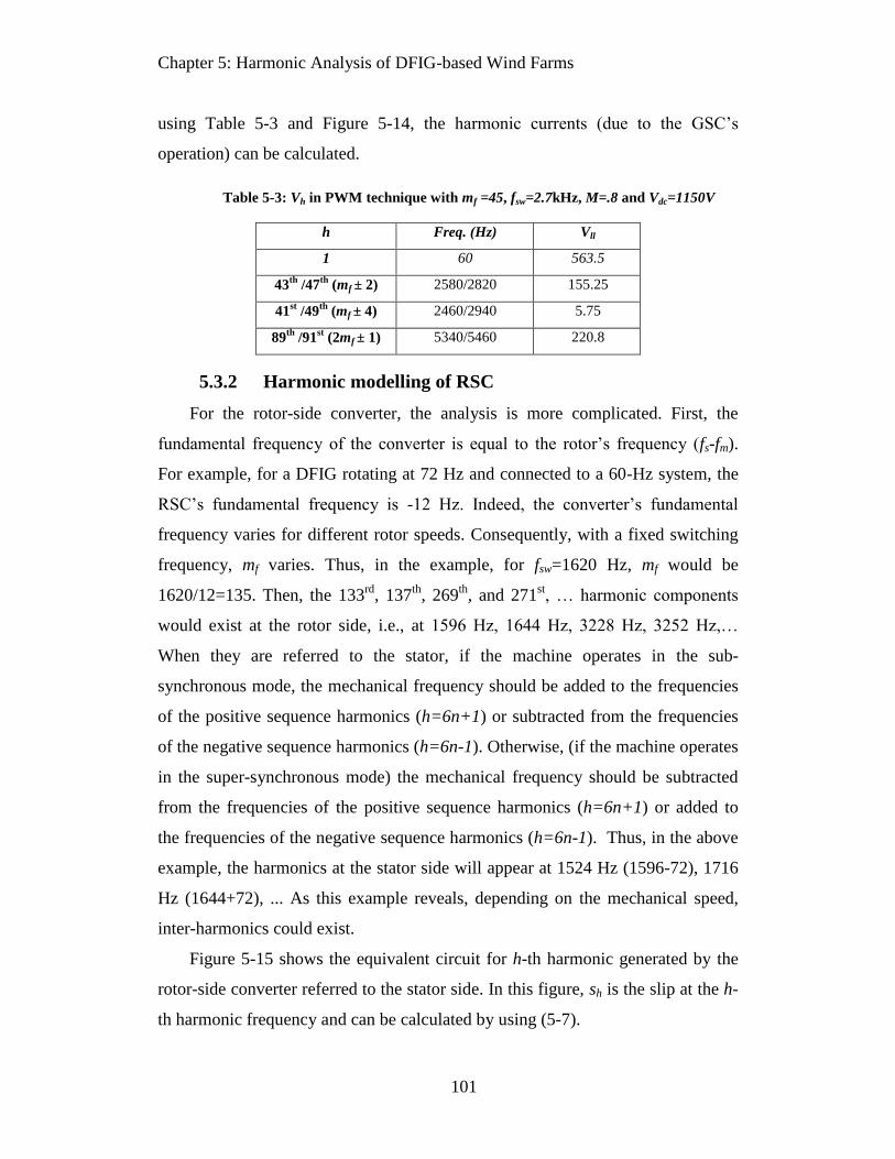
Chapter 5: Harmonic Analysis of DFIG-based Wind Farms
101
using Table 5-3 and Figure 5-14, the harmonic currents (due to the GSC’s
operation) can be calculated.
Table 5-3: Vh in PWM technique with mf =45, fsw=2.7kHz, M=.8 and Vdc=1150V
h Freq. (Hz) Vll
1 60 563.5
43th
/47th
(mf ± 2) 2580/2820 155.25
41st /49
th (mf ± 4) 2460/2940 5.75
89th
/91st (2mf ± 1) 5340/5460 220.8
5.3.2 Harmonic modelling of RSC
For the rotor-side converter, the analysis is more complicated. First, the
fundamental frequency of the converter is equal to the rotor’s frequency (fs-fm).
For example, for a DFIG rotating at 72 Hz and connected to a 60-Hz system, the
RSC’s fundamental frequency is -12 Hz. Indeed, the converter’s fundamental
frequency varies for different rotor speeds. Consequently, with a fixed switching
frequency, mf varies. Thus, in the example, for fsw=1620 Hz, mf would be
1620/12=135. Then, the 133rd
, 137th
, 269th
, and 271st, … harmonic components
would exist at the rotor side, i.e., at 1596 Hz, 1644 Hz, 3228 Hz, 3252 Hz,…
When they are referred to the stator, if the machine operates in the sub-
synchronous mode, the mechanical frequency should be added to the frequencies
of the positive sequence harmonics (h=6n+1) or subtracted from the frequencies
of the negative sequence harmonics (h=6n-1). Otherwise, (if the machine operates
in the super-synchronous mode) the mechanical frequency should be subtracted
from the frequencies of the positive sequence harmonics (h=6n+1) or added to
the frequencies of the negative sequence harmonics (h=6n-1). Thus, in the above
example, the harmonics at the stator side will appear at 1524 Hz (1596-72), 1716
Hz (1644+72), ... As this example reveals, depending on the mechanical speed,
inter-harmonics could exist.
Figure 5-15 shows the equivalent circuit for h-th harmonic generated by the
rotor-side converter referred to the stator side. In this figure, sh is the slip at the h-
th harmonic frequency and can be calculated by using (5-7).

Chapter 5: Harmonic Analysis of DFIG-based Wind Farms
102
Rs Ls
Lm
L’r
Vs,h
R’r / sh
V’r,h / sh
Figure 5-15: DFIG’s equivalent circuit at hth harmonic frequency
(1 ), (6 1)
(1 ), (6 1)
h
h
h ss h k
h
h ss h k
h
(5-7)
Since h is relatively large and -.3<s<.3, sh≈1. Also, the magnetization branch
can be neglected. As a result, for harmonic studies, the RSC can be modeled as
shown in Figure 5-16. Similar to the GSC, amplitudes of harmonic voltages can
be obtained by using (5-2). In addition, when the harmonic voltages are referred
to the stator side, their amplitudes should be multiplied by the stator-to-rotor turn
ratio.
Vh(M, Vdc)
h(X’r+Xs) (R’r+ Rs)
Rc
hXcNetwork
Rf
Xf/h
Figure 5-16: Harmonic modelling of RSC at its hth harmonic
5.4 Simulation
In order to investigate the validity of the proposed harmonic model, a power
system with a DFIG-based wind farm was simulated in MATLAB/Simulink. In
the following paragraphs, the simulated system is introduced, and the simulation
results are presented and compared with the results obtained from the harmonic
modelling of DFIG.
5.4.1 Simulated system
The simulated system was prepared by Hydro-Quebec and presented as a
demo in Simulink. Figure 5-17 shows the simulated system, and Figure 5-18

Chapter 5: Harmonic Analysis of DFIG-based Wind Farms
103
shows the details of the DFIG wind farm. As Figure 5-17 reveals, the wind farm is
connected to a 120 kV system via a 30 km 25 kV feeder. The wind farm consists
of 6 DFIGs with rated voltage of 575 V and rated power of 1.5 MW (9MW total).
As Figure 5-18 reveals, the GSC is connected to the grid through an inductor
while the RSC is directly connected to the rotor. Also, a 120 kVAR shunt filter is
connected to the stator’s terminals of each DFIG (720kVar total). The main
functional of these elements is to filter the high-frequency harmonic current and
not to provide reactive power. A detailed representation of power electronics
converters is used in this model. The PWM GSC’s and RSC’s switching
frequencies are 2700 Hz and 1620 Hz, respectively. During the simulation, the
wind speed is 15 m/s, which rotates the DFIG’s rotor at 1.2 time the synchronous
speed (s=-.2).
Figure 5-17: Simulated power system
I1
I2
I3
I4I5
Figure 5-18: Details of wind farm simulation

Chapter 5: Harmonic Analysis of DFIG-based Wind Farms
104
120 kV network
Z1=(.1+j)p.u., Z0=3 Z1, Sbase=2500MVA
120kV/25kV transformer
Srated=47MVA, X1=X2=0.08p.u., X/R=30, Yg/D
Grounding transformer
Srated =100MVA, Z0=(.025+j0.75)p.u.
25kV feeder
r1=.1153 Ω/km, r0=.413 Ω/km, l1=1.05 mH/km, l0=3.32 mH/km, c1=11.33 pF/km,
c0=5.01 pF/km, Length: 30 km
Wind farm’s transformer
Srated =10.5MVA, X1=X2=0.025p.u., X/R=30
DFIGs
Wind farm includes 6 parallel 1.5 MW DFIGs. For each DFIG: PFrated=.9,
Rs=.023 p.u., R'r=.016 p.u., Xs=.18 p.u., X'r=.16 p.u., Xm=2.9 p.u.,
Rchoke=.003p.u., Xchoke=.3 p.u.
Shunt filter for each turbine
Qrated=120kVar, Quality factor (
)=50,(R=.0551 Ohm, C=936uF ωc=3kHz.)
5.4.2 Simulation results
Figure 5-19 shows the DC link voltage obtained from the simulation. As this
figure reveals, the DC voltage contains ripples. However, the magnitude of the
ripples never exceeds 0.005 of the DC component. Therefore, the assumption of
constant DC link voltage was reasonable for the harmonic modelling.

Chapter 5: Harmonic Analysis of DFIG-based Wind Farms
105
Figure 5-19: DC link voltage
Figure 5-20 shows the normalized harmonic spectrum of the GSC’s current
(I1 in Figure 5-18). As this figure reveals, the major harmonics are the odd
sidebands of the GSC’s switching frequency (mf=2700/60=45), which are 43rd
and 47th
, and also the sidebands of its multiples, which are 89th
and 91st.
Figure 5-23 shows the normalized harmonic spectrum of the RSC’s current
(I2). As this figure reveals, the major harmonics are the odd sidebands of RSC’s
switching frequency (mf=1620/12=135), which are 133rd
(1596 Hz) and 137th
(1644 Hz), and also the sidebands of its multiples, which are 269th
and 271st. Note
that the fundamental current is at -12 Hz (f1,rotor=s*f1,system). Moreover, there is no
sign of interaction between the RSC and GSC in the harmonic spectrum.
Figure 5-20: Harmonic spectrum of GSC’s current (% of converter’s fundamental current)
0 1/600.995
1
1.005
Time (sec.)
Vd
c (
norm
aliz
ed)
0 20 40 60 80 1000
20
40
60
80
100
X = 43Y = 16.1
Harmonic order
Harm
onic
conte
nt (%
of fu
ndam
enta
l)
X = 47Y = 14.8 X = 89
Y = 9.67X = 91Y = 9.37

Chapter 5: Harmonic Analysis of DFIG-based Wind Farms
106
Figure 5-21: Harmonic spectrum of GSC’s current (% of generator’s fundamental current)
Figure 5-22: Harmonic spectrum of RSC’s current (% of converters fundamental current,
fundamental frequency=12 Hz)
Figure 5-23: Harmonic spectrum of RSC’s current (% of generator’s fundamental current)
Another way to justify the decoupling of the DC link in the modelling is to
compare the simulation results with the case in which the DC link’s capacitor is
replaced by an ideal DC voltage source in the presence of the background
harmonic voltages in the grid. To do so, 1% background 43rd
and 47th
harmonic
voltages and .5% 89th
and 91st harmonic voltages were embedded in the simulated
system. Table 5-4 and
0 20 40 60 80 1000
4
8
12
16
Harmonic order
Harm
onic
conte
nt (%
of fu
ndam
enta
l)
X=43Y=2.57
X=47Y=2.36 X=89
Y=1.53X=91Y=1.48
100 150 200 250 3000
5
10
Harmonic orderHarm
onic
com
ponent (%
of fu
ndam
enta
l)
X=135Y=2.29
X=133Y=2.37
X=269Y=3.27
X=271Y=3.22
100 150 200 250 3000
1
2
3
4
5
Harmonic orderHarm
onic
com
ponent (%
of fu
ndam
enta
l)
X = 133Y = 0.653
X = 137Y = 0.629
X = 269Y = 0.9
X = 271Y = 0.886

Chapter 5: Harmonic Analysis of DFIG-based Wind Farms
107
Table 5-5 show this comparison for the harmonic spectra of GSC and RSC,
respectively, with and without background harmonics. Diff.1 shows the
differences without background harmonics and Diff.2 shows the differences with
background harmonic voltages. As these tables reveal, the differences are
negligible and, consequently, the assumption that the RSC and GSC are
decoupled harmonic sources is valid.
Table 5-4: Major harmonic components of GSC current
h
Harmonic content (% of converter’s fundamental component) Diff.1
(%)
Diff.2
(%) DC link with capacitor DC link with ideal voltage source
no background With background no background With background
43 16.5 16.6 16.5 16.5 0 .6
47 15.1 14.3 15.3 14.2 1.3 .7
89 9.87 9.94 9.84 1 .3 1
91 9.61 9.73 9.65 9.71 .4 .2
Table 5-5: Major harmonic components of RSC current
h
Harmonic content (% of converter’s fundamental component) Diff.1
(%)
Diff.2
(%) DC link with capacitor DC link with ideal voltage source
no background With background no background With background
133 .649 .652 .65 .652 .1 0
137 .622 .626 .624 .627 0.3 .2
269 .907 .907 .905 .907 0 0.2
271 .901 .903 .901 .901 0.2 0
Figure 5-24 shows the normalized harmonic spectrum of the stator’s current
(I3). As this figure reveals, very small 43th
and 47th
harmonics appear in the
stator’s current, which are the results of the GSC’s switching. On the other hand,
the major harmonics in the stator currents are 1524, 1716, 3180 and 3300 Hz,
which are induced by the RSC. As was explained in the previous section, the 1524
Hz component is the 1596 Hz component of the RSC which is induced to the
stator and the rotor’s mechanical frequency (72 Hz) is deducted (1524 = 1596-72).
Likewise, the 1716 Hz component in the stator’s current is actually the 1644 Hz

Chapter 5: Harmonic Analysis of DFIG-based Wind Farms
108
component of the RSC induced in the stator, and the rotor’s mechanical frequency
(72 Hz) is added (1716 = 1644+72).
Figure 5-24: Harmonic spectrum of stator’s current
Figure 5-25 shows the normalized harmonic spectrum of the wind farm’s
current before the shunt filter (I4). As this figure reveals, this current contains
harmonics from the GSC and also from the RSC, induced in the stator.
Figure 5-25: Harmonic spectrum of I4
Figure 5-26 shows the normalized harmonic spectrum of the wind farm’s
output current I5 (after the shunt filter). As this figure reveals, because of the
shunt filter, this current contains very low harmonics components (the largest
component is 0.26% of the fundamental).
20 30 40 50 60 70 80 90 1000
1
2
3
4
5
X = 91Y = 1.48
X = 89Y = 1.53
Harmonic orderHarm
onic
com
ponent (%
of fu
ndam
enta
l)
X = 55Y = 0.808
X = 53Y = 0.812
X = 47Y = 2.36
X = 43Y = 2.58
X = 28.6Y = 0.466
X = 25.4Y = 0.505

Chapter 5: Harmonic Analysis of DFIG-based Wind Farms
109
Figure 5-26: Harmonic spectrum of I5
Figure 5-27 shows the harmonic spectrum of the line-to-line voltage at the
wind farm’s connection point (the 575V side of the transformer). As this figure
reveals, the magnitude of any harmonic component does not reach 1% of the
fundamental component.
Figure 5-27: Harmonic spectrum of voltage
5.4.3 Comparison of the results
In this subsection, two sets of harmonic components of currents at two
frequencies are presented as examples. One set is obtained from the detailed
simulation and the other set is obtained from the proposed harmonic model of
DFIG (Figure 5-35). These sets are compared to show the validity and accuracy of
the proposed harmonic model. Note that for harmonic modelling, the amplitude of
harmonic voltage sources in Figure 5-35 should be calculated from (5-2). In this
case study, Vdc=1150V, MGSC=.82, MRSC=.59.
20 30 40 50 60 70 80 90 100
0.5
1.5
2.5
X = 43Y = 0.0981
Harmonic orderHarm
onic
com
ponent (%
of fu
ndam
enta
l)
X = 79.4Y = 0.152
X = 47Y = 0.122
X = 89Y = 0.223
X = 91Y = 0.258
20 30 40 50 60 70 80 90 100
0.5
1.5
2.5
X = 25.4Y = 0.289
Harmonic order
Harm
onic
conte
nt (%
of fu
ndam
enta
l)
X = 28.6Y = 0.238
X = 43Y = 0.952 X = 47
Y = 0.813
X = 53Y = 0.257
X = 55Y = 0.254
X = 91Y = 0.373
X = 89Y = 0.413

Chapter 5: Harmonic Analysis of DFIG-based Wind Farms
110
Vham,GSC
h(X’r+Xs) (R’r+ Rs)
Rf
Xf/h
Network Rc
hXc
Vham,RSC
Figure 5-28: Equivalent DFIG model
The studied frequencies are 2580 Hz and 3300 Hz. The current components at
2580 Hz ((mf,GSC-2)*60Hz) are caused by the GSC, while the components at 3300
Hz ((2m f,RSC-1)*12Hz+72Hz) are caused by the RSC.
For the 2580 Hz components, since they are caused by the GSC, the model in
Figure 5-14 should be used to calculate the currents. From (5-2),
Vll,43th=.1405*1150=161.58 V. Table 5-6 shows the 2580 Hz current components
obtained from the simulation and modelling. As this table reveals, the results from
the modelling are in close agreement with the results from the simulation.
Table 5-6: Harmonic components at 2580 Hz
RMS Harmonic component (A)
Modelling Simulation
GSC current (I1) 165.21 163.01
Stator current (I3) 4.77 5.62
Wind farm output current before shunt filter (I4) 168.85 167.76
Current injected to the grid (I5) 6.34 6.37
For the 3300 Hz components, since they are caused by the RSC, the model in
Figure 5-16 should be used to calculate the currents. From (5-2), Vll,269h
=.2268*1150=260.82 V, which should be referred to stator side V’ll,269h =260.82
V*ns/nr =75.94V. Table 5-7 shows the 3300 Hz current components obtained
from the simulation and modelling. As this table reveals, the results from the
modelling are in close agreement with those from the simulation.

Chapter 5: Harmonic Analysis of DFIG-based Wind Farms
111
Table 5-7: Harmonic components at 3300 Hz
RMS Harmonic component (A)
Modelling Simulation
GSC current (I1) 1.5525 2.4
Stator current (I3) 50.78 50.62
Wind farm output current before shunt filter (I4) 51.56 52.32
Current injected to the grid (I5) 4.51 4.47
5.5 Estimation of parameters
In previous sections, it was shown that all harmonic voltages and currents
caused by a DFIG-based wind farm can be calculated by knowing Vdc and the
amplitude modulation ratios of the DFIG’s converters (MGSC and MRSC). The main
aim of this section is to propose methods to estimate typical values for Vdc, MGSC
and MRSC in a DFIG-based wind system. For this purpose, the stator and rotor
powers in the steady state operation of DFIG systems must be estimated. In the
following sub-sections, the steady state operation of DFIG systems is studied, and
estimations for Vdc, MGSC and MRSC are presented.
5.5.1 Stator and rotor powers
The mechanical power extracted by a wind turbine at wind speed can be
expressed as follows [77]:
3( )2
mech pP c Av
(5-8)
where ρ is specific air mass, A is the circular swept area, and cp is the power
coefficient. As (5-8) reveals, cp is a function of the tip speed ratio λ, which is the
ratio of the circumferential velocity of the turbine’s blade tips and the wind speed.
Figure 5-29 shows a typical cp over λ curve. As this figure reveals, there is a tip
speed ratio at which cp has its maximum value. In other words, from this curve,
we can find a rotor speed/slip at which the turbine produces maximum power at a
certain wind speed. After determining this rotor speed, the optimum turbine
torque can be obtained from (5-9). One of the main functions of the RSC

Chapter 5: Harmonic Analysis of DFIG-based Wind Farms
112
controller is to control the rotor voltage so that machine operates at this torque to
ensure maximum wind power extraction.
maxem
mech
P
(5-9)
Figure 5-29: A typical cp over λ curve
Figure 5-30 shows the power sharing between the stator and rotor in the
DFIG system where the losses are neglected [77]. As this figure reveals, the stator
power ( ) and rotor power ( ) can be obtained as follows:
r sP sP (5-10)
and
(1 )mech s r sP P P s P (5-11)
As a result,
1
(1 )s mechP P
s
(5-12)
and
(1 )r mech
sP P
s
(5-13)
Pmech Ps
Pr=sPs
Pmech
Figure 5-30: Power sharing in a loss-less DFIG system
0 2 4 6 8 10 12 140
0.1
0.2
0.3
0.4
0.5
Lambda
cp

Chapter 5: Harmonic Analysis of DFIG-based Wind Farms
113
5.5.2 Estimation of Vdc and MGSC
The main function of the GSC is to maintain the dc link voltage at a constant
level by controlling the active power exchange between the network and DC link.
Figure 5-31 shows the equivalent circuit of the GSC at the fundamental frequency
during steady state. Note that in this figure, the series filter’s resistance is
neglected.
V1 δ
Xf
Network1 0
Figure 5-31: Equivalent circuit of GSC at fundamental frequency during steady state
The active and reactive powers transferred to the network can be expressed as
1 sinGSC
f
VP
X (5-14)
1 cos 1GSC
f
VQ
X
(5-15)
For unity power factor operation, 0GSCQ . therefore:
1
1
1cos
V (5-16)
From (15) and (17)
2
1 ( ) 1f GSCV X P (5-17)
and since at steady state GSC rP P
2
1 ( ) 1f rV X P (5-18)
Thus, at an average wind speed, the GSC’s fundamental voltage is obtained from
(5-18). On the other hand,

Chapter 5: Harmonic Analysis of DFIG-based Wind Farms
114
1
3
2 2GSC dcV M V (5-19)
Therefore,
2( ) 12 2
3
f r
dc
GSC
X PV
M
(5-20)
As (5-20) reveals, there is only one equation for the two unknowns, Vdc and
MGSC, so, one of these parameters can be selected freely. For MGSC, 0< MGSC <1,
and a higher MGSC results in a lower dc link voltage (and, therefore, simpler and
less costly implementation). However, an MGSC close to 1 should be avoided to
minimize the chance of overmodulation. As a result, MGSC ≈.8 is a reasonable
assumption. Then, Vdc is obtained from (5-20).
5.5.3 Estimation of MRSC
In subsection 5.5.1, the optimum torque (at which maximum power
extraction happens) was obtained. Now, the rotor voltage referred to the stator
side at this torque is obtained as follows [79]:
2 2
2 2
3 3
s em s r s s s rrr r
s m s m s m
L L V Q L LLV
pV L L V L
(5-21)
where Ls and Lr are the stator and rotor inductances, respectively; Lm is the mutual
inductance; and σ is the leakage factor (2
1 m
s r
L
L L ).
At the unity power factor operation
2 2
3
s em s r s rr r
s m s m
L L V LV
pV L L
(5-22)
Now, the voltage at the RSC can be obtained as follows:
2 2
3
s em s r sr rRSC r
s s m s m
L L VN LV
N pV L L
(5-23)
Finally, from the PWM principles, can be obtained as follows:
2 2
3
RSCGSC
dc
VM
V (5-24)

Chapter 5: Harmonic Analysis of DFIG-based Wind Farms
115
Now all the parameters required to calculate the harmonic voltages and
currents are available. By calculating these parameters at an average wind speed
and using them in the method proposed in the modelling section, the typical
harmonic spectra of the voltages and currents can be obtained for a DFIG-based
wind farm.
5.6 Illustrative example
5.6.1 Study scenario
In the previous section, a method was proposed to estimate the average
harmonics in a DFIG-based wind system. However, an average wind speed and a
cp over λ curve were required for that method. In this sub-section, rough
estimations for MGSC and MRSC are provided to determine the worst case in terms
of harmonics. In contrast to previous section, there is no need to have wind speed
or turbine specifications data.
In the worst case, both the GSC and RSC produce maximum harmonic
voltages at the lowest harmonic frequencies, which are the first sidebands of the
switching frequencies ( 1fm ). Figure 5-32 shows the normalized amplitude of
these components for different values of the amplitude modulation ratio in a
sinusoidal PWM switching scheme. This figure is obtained from (5-3).
Figure 5-32: Normalized amplitude of mf-1-th harmonic for different values of M
As Figure 5-32 reveals, the amplitude of the lowest-frequency harmonic is
increased by increasing the amplitude modulation ratio. As a result, for estimating
the worst case, MGSC = 1 and MRSC = 1 can be considered.
0 0.2 0.4 0.6 0.8 1
0.05
0.1
0.15
0.2
Amplitude modulation ratio (M)
No
rma
lize
d a
mp
litu
de

Chapter 5: Harmonic Analysis of DFIG-based Wind Farms
116
5.6.2 Example
In this sub-section, an example is provided to illustrate the procedure for
determining the major harmonic components in the worst-case scenario.
In this example, it is known that 6 DFIGs (1.5 MW each, PF=.9) are
connected to a collector bus. The desirables are the major harmonic current
components injected into the grid by GSC in the worst-case scenario. The
estimation procedure consists of the following steps:
0. The following parameters should be known:
a. The converter’s switching frequencies (in this example, fsw=2.7kHz)
b. The DC link voltage (in this example Vdc=1150V)
c. The ratio of the stator and rotor rated voltages (or stator-to-rotor turn
ratio)
d. The machine’s total rotor and stator resistances and reactances (in this
example p.u. and
p.u.)
e. The choke’s reactance and resistance (in this example, p.u.
and p.u. Note that normally, ≪ , so may be
neglected.)
f. Filter’s resistance and capacitor (in this example and
)
1. Calculate the impedances in the equivalent circuit of Figure 5-33 from
the known parameters listed in the previous step:
(for 6 parallel DFIGs)
(equivalent for 6 parallel filters)

Chapter 5: Harmonic Analysis of DFIG-based Wind Farms
117
(equivalent for 6 parallel filters)
2. Determine the harmonic order and amplitudes for harmonic voltage
source of Figure 5-33:
a. Determining frequency modulation ratio:
,
b. Determining harmonic orders: these components are sidebands of mf
and 2mf, i.e., h=mf±2 (43rd
and 47th
), and h=2mf±1(89th
and 91st)
c. Determining harmonic voltage amplitudes: in 5.2, it was shown that
Vll,h = k Vdc where k is the coefficient of double Fourier series and can
be obtained from either equation 5.4 or by using Table 5-2, which is
repeated below. In this example, Vdc=1150V is multiplied by .195 to
obtain Vll,43 and Vll,47. Therefore, Vll,43 = Vll,47 = .195*1150 = 224.25
V. Similarly, Vdc is multiplied by .111 to obtain Vll,89 and Vll,91.
Therefore, Vll,89 = Vll,91 = .111*1150 = 127.65 V.
Vh/Vdc in PWM technique with large odd mf multiple of 3
h M
.2 .4 .6 .8 1
1 .122 .245 .367 .490 .612
mf ± 2 .010 .037 .080 .135 .195
mf ± 4 - - - .005 .011
2mf ± 1 .116 .200 .227 .192 .111
2mf ± 5 - - - .008 .020
3mf ± 2 .027 .085 .124 .108 .038
3. Calculate the harmonic currents: for each harmonic order h, the
corresponding Vll,h obtained in the previous step is considered in the
equivalent circuit of Figure 5-33, and the current injected into the
network (ih) is calculated. Table 5-8 shows the harmonic current
spectrum of this example.

Chapter 5: Harmonic Analysis of DFIG-based Wind Farms
118
Vll,h
h(X’r+Xs) (R’r+ Rs)
Rf
Xf/h
Network Rc
hXc
ih
Figure 5-33: Equivalent circuit for calculation of harmonic currents caused by GSC
Table 5-8: Major harmonic components the example in the worst condition
Harmonic order (h) Harmonic content (% of fundamental)
43 .147
47 .1762
89 .4906
91 .578
Note that to calculate the harmonic current caused by the RSC, the procedure
is similar except for two slight differences: (a) in Step 2, the harmonic voltages
should be multiplied by the ratio of the stator’s rated voltage to the rotor’s rated
voltage or the stator-to-rotor turn ratio (in order to convert the harmonic voltage
source from the rotor circuit to the stator circuit), and (b) instead of using
equivalent circuit of Figure 5-33, the equivalent circuit shown in Figure 5-34
should be used.
Vll,h
h(X’r+Xs) (R’r+ Rs)
Rf
Xf/h
Network Rc
hXc
ih
Figure 5-34: Equivalent circuit for calculation of harmonic currents caused by RSC
5.7 Non-characteristic harmonics
In the modelling, the DC link voltage was considered to be ripple-free and,
consequently, only the harmonics due to the ideal PWM switching was considered

Chapter 5: Harmonic Analysis of DFIG-based Wind Farms
119
in the model. However, in 5.1 it was shown that low-order non-characteristic
harmonics are also present in the converters’ terminal voltages. This section will
demonstrate the source of these components.
Figure 5-35 (a) shows the normalized harmonic contents of the GSC’s
terminal voltage. As this figure reveals, the main components are the sidebands of
the switching frequency (the 43rd
and 47th
order harmonics). However, small but
non-zero components exist at lower frequencies. Figure 5-35 (b) reveals that these
components have magnitudes of less than 0.8% of the fundamental component’s
magnitude. These results were achieved when no background distortion was
present in the distribution system. Consequently, they are caused by the
converters and their control system.
(a)
(b)
Figure 5-35: Normalized harmonic components of voltage at GSC terminals, (a) up to 48th
harmonic, (b) up to 21st harmonic
Figure 5-36 shows the reference signal generated by the GSC’s controller,
and Figure 5-37 shows its harmonic spectrum. As these figures reveal, the
converter’s controller fails to generate a purely sinusoidal reference signal, and
this signal contains harmonics which are modulated with the carrier signal and
appear in the converter’s voltages. Nevertheless, as was mentioned above, the
magnitude of these harmonics is very small, and the main aim of this section was
to demonstrate only the origin of these components.
0 5 10 15 20 25 30 35 40 45
0.1
0.2
.3
Harmonic order
Am
plit
ud
e (
p.u
.)
3 9 15 21
.01
Harmonic order
Am
plitu
de
(p
.u.)

Chapter 5: Harmonic Analysis of DFIG-based Wind Farms
120
Figure 5-36: PWM reference signal of GSC
Figure 5-37: Normalized spectrum of PWM reference signal of GSC
5.8 Comparison with other harmonic sources and standards
It is advantageous to quantitatively compare the harmonic emissions of
DFIG-based wind farms with those of more well-studied and well-characterized
harmonic sources and also with the harmonic limits suggested by power quality
standards. Such comparisons will provide a better understanding of the amount of
harmonics emitted by DFIG-based wind farms.
In [80] the equivalent-CFL indexing method is proposed to compare
harmonic emissions of home appliances. In this method, the current harmonics of
CFLs are considered as a “relative harmonic injection benchmark” for comparing
the harmonic injections of other home appliances [80]. Then, the equivalent CFL
index is calculated for each appliance. The CFL index of each appliance expresses
the harmonic emissions of that appliance as the number of CFLs its harmonic
emissions are equivalent to. The procedure to obtain the equivalent CFL index is
as following [80]:
1. For each harmonic order, the ratio of appliance’s current ( )
to the CFL’s current ( ) is calculated:
0 .025 .05-1
-0.5
0
0.5
1
time (s)
0 200 400 600 800 1000 12000
1
2
3
4
5
6
7
8x 10
-3
Frequency (Hz)
Ha
rmo
nic
co
nte
nt

Chapter 5: Harmonic Analysis of DFIG-based Wind Farms
121
,
,
,
h appliance
h appliance
h CFL
IRatio
I (5-25)
2. The ratios are aggregated to one value as follows:
2
,
3
2
,
3
2
,
3
( * )H
h h appliance
h
H
h appliance
h
H
h CFL
h
Equivalent CFL w Ratio
I
I
(5-26)
where the weighting factor hwis the individual harmonic distortion of
the CFL’s current [80].
Although the equivalent CFL indexing is an appropriate method for
comparing the low frequency harmonic injection of relatively small appliances
but not wind farms, the idea can be borrowed, and larger harmonic sources such
as Plug-in Hybrid Electric Vehicle (PHEV) chargers, service transformers, and
DC drives can be used as benchmarks instead of CFLs. In the following
paragraphs, by using (5-26), the harmonic emissions of the simulated DFIG-based
wind farm are quantitatively compared to above mentioned sources. Note that this
method has been established for low-frequency harmonics and only the low-
frequency harmonic components of the benchmarks’ spectra are available for
comparison. Nevertheless, such comparison provides a useful insight into the
level of the wind farm’s non-characteristic harmonics.
Table 5-9: Normalized spectrum of harmonic sources
Sourc
e Ih3 Ih5 Ih7 Ih9 Ih11 Ih13 Ih15 Ih17 Ih19 Ih21 Ih23 Ih25 Ih27 Ih29
PHEV 0.042
4
0.001
2
0.001
9
0.001
2
0.001
5
0.002
4
0.004
1
0.002
1
0.001
5
0.000
5
0.000
8
0.001
8
0.001
5
0.001
1
ST*
0 0.131
5 .057 0 0.019
0.015
6 0 0.008
0.003
9 0
0.006
1
0.003
1 0
0.001
1
DCD**
0.023 0.017 0.008 0.005 0.073
4
0.042
1 0.003 0.007
0.005
5
0.003
1
0.012
4
0.013
2 0.003
0.002
8
* ST: Service transformer
** DCD: DC drive
Table 5-9 shows the normalized spectra of a type-2 PHEV charger, a 37 kVA
service transformer and a 12-pulse DC drive obtained from measurements. These
values are used in (5-26) instead of the CFL’s harmonic currents. As a result,

Chapter 5: Harmonic Analysis of DFIG-based Wind Farms
122
three indices are obtained for the wind farm, which are .085 in comparison to the
PHEV charger, 0.0254 in comparison to the service transformer and 0.04 in
comparison to the DC drive. These values are all smaller than 1. Therefore, the
wind farm is not a significant source of harmonic emissions in comparison to
these three sources. For further illustration, consider a 9MW wind farm and a 3-
kW type-2 PHEV charger. The wind farm’s power is 3000 times the charger’s
power while its harmonic injection is equal to only 3000*.085=255 of the PHEV
chargers’ injections. Similarly, the wind farm’s power is almost 243 times that of
the service transformer (which normally feeds 243*10 house/transformer=2430
houses) while its harmonic injection is equal to only 243*.0254=6.17 of the
service transformers’ (62 houses’) injection.
In this part of the research, the harmonic emissions of wind farms were also
compared with the harmonic limits specified in the major power quality standards,
IEEE Std. 1547 and IEC 61000-3. In contrast to the equivalent CFL indexing, the
comparison of the DFIG’s harmonic spectrum with the limits determined in these
standards provides the opportunity to assess the high-frequency harmonic
emissions of the wind farms. Table 5-10 shows the comparison between the
current harmonic emissions from the simulated wind farm with the limits
determined in IEEE Std. 1547. As this table reveals, the simulated wind farm
complies with the limits in the standard.
Table 5-10: Comparison of the farm’s harmonic currents with the limits of IEEE Std. 1547
Source Ih5
(%)
Ih7
(%)
Ih11
(%)
Ih13
(%)
Ih17
(%)
Ih19
(%)
Ih23
(%)
Ih25-33
(%)
Ih>33*
(%)
DFIG .34 .04 .07 .02 .005 .004 .001 - .258
IEEE Std.
1547 4 4 2 2 1.5 1.5 .6 .6 .3
* According to Figure 5-26 for h>33, the highest harmonic content of the simulated wind system is
0.258%
Table 5-11 shows the comparison between the voltage harmonics at the wind
farm’s PCC with the limits specified by IEC 61000-3. As this table demonstrates,
the wind farm’s operation complies with IEC 61000-3.
Table 5-11: Comparison of the farm’s harmonic voltages with the limits of IEC 61000-3

Chapter 5: Harmonic Analysis of DFIG-based Wind Farms
123
Source Vh5
(%)
Vh7
(%)
Vh11
(%)
Vh13
(%)
Vh17
(%)
Vh19
(%)
Vh23
(%)
Vh25
(%)
Vh43
(%)
Vh47*
(%)
DFIG .06 .02 .02 .15 .22 .04 .01 .06 .952 .813
IEC 61000-3
5 4 3.5 3 2 1.5 1.5 1.5 .96 .89
* For h>25, the IEC 61000-3 limit is calculated as 0.2+1.3*(25/h). For the simulated system,
harmonic components for h>47 also comply with IEC 61000-3.
5.9 Conclusion
In this chapter, the harmonic emissions of DFIG-based wind farms were
analyzed, and a harmonic modelling method was proposed. The following points
are the main conclusions of this chapter.
1. An accurate model was presented based on a double Fourier series of
the sinusoidal PWM pulse train, and validated by using time-domain
simulations. The model contains only voltage sources and impedances
and can be used instead of a detailed power electronic model for
harmonic analysis.
2. It was shown that DFIG-based wind systems generated both
harmonics and inter-harmonics. The frequency of inter-harmonics
depends on the rotor’s speed, which is a function of wind speed.
3. In PWM switching, the harmonics appear in the odd sidebands of the
converters’ switching frequencies. The simulations and analysis
showed that DFIGs converters generated large characteristic harmonic
currents and voltages. However, the DFIG is equipped with a filter
which prevents the propagation of harmonics in the network. As an
example, in the simulated case, the normalized amplitude of the
harmonic currents injected to the PCC is less than .3%, and the
normalized amplitude of each harmonic voltage at PCC was less than
1%.
4. The detailed simulations showed that non-characteristic harmonics
can appear in the DFIG’s output, which are caused by converters’
control systems. These non-characteristic harmonic components
appear in the lower frequencies (lower than 1kHz).

Chapter 5: Harmonic Analysis of DFIG-based Wind Farms
124
5. The sensitivity analysis showed that these non-characteristic
harmonics were changed arbitrarily by the change in the power
system’s background harmonic spectrum. Especially, referring to
Figure 5-8, the low-order integer-harmonics which are the most
important components in harmonic studies, show almost no sensitivity
to the background harmonics.
6. Finally, the characteristic and non-characteristic harmonic
components of a DFIG system have very low magnitudes. As a result,
these components can barely be considered as harmonic sources in the
power system. This finding was confirmed by the quantitative
comparison of the harmonic emissions of the DFIG-based wind farms
with those of other harmonic sources.

Chapter 6: Conclusions and Future Work
125
Chapter 6
Conclusions and Future Work
In this chapter, the main findings of the thesis are summarized, and
suggestions for future work are presented.
6.1 Thesis conclusions and contributions
This thesis investigated the impact of DGs on the O.C. protection system’s
coordination and also on DG’s harmonic emissions. The conclusions and
contributions are as following:
The potential impact of DGs on the O.C. protection were illustrated. This
impact causes miscoordination between the main and back-up protection
devices, failure in the fuse-saving scheme, false tripping, and desensitization
of the protection. As well, the magnitude of the fault current contributed by a
DG and the time widow during which the DG’s fault current contribution is
significant were identified as two key factors which should be considered
during an investigation of the impact of each DG type on the coordination.
DGs were categorized into four types based on their electrical interface with
the power system. The early stages of the research showed that Induction-
Machine DGs (IMDG) and Permanent Magnet Synchronous Generators
(PMSGs) had a negligible impact on the O.C. coordination. The findings on
these two types are available in the appendices. Consequently, the main focus
was on the IBDGs and SMDGs and finding methods to mitigate their impact
on the O.C. coordination.
Regarding IBDGs, it was shown that IBDGs with DG trip protection cannot
impact on the coordination. In contrast, IBDGs with current-limiting

Chapter 6: Conclusions and Future Work
126
protection may impact on the marginal coordinations, especially at relatively
high penetration levels. In order to mitigate this impact, a strategy was
proposed in which the inverter’s current limit is not fixed but adjusted
dynamically based on the PCC voltage. The simulation results showed that, by
using the proposed control strategy, the inverter’s current was limited
significantly when a fault happened near the PCC. As a result, the simulated
IBDG had no contribution to the fault and could not impact on the
coordination. In addition, by this strategy when non-fault disturbances or
distant faults occurred (where DG has no impact), IBDG operated normally.
In summary, this strategy can be implemented easily and can mitigate the
probable impact of IBDGs on coordination successfully without causing any
abnormal operation during the power system’s normal operation or non-fault
disturbances.
It was shown that among all types of DGs, SMDGs had the highest and the
longest contribution to the fault current. The machine’s response was divided
into three periods, and it was shown that during the transient period,
machine’s fault current was 3~5 p.u. which gradually decayed with a transient
time constant in the range of 1-2 sec. This period coincided with the operation
of major O.C. devices in distribution system, and this part of machine’s
response seriously impacted on the coordination. Next, in order to restrict the
machine’s fault current contribution in this period and, consequently, to
mitigate the impact of the machine on the O.C. protection coordination, a field
discharge application was proposed. The mathematical analysis and
simulation result showed that this circuit removed the steady state part of
machine’s current by disconnecting its excitation and decreased the machine’s
transient time constant by increasing field circuit’s resistance. As a result, the
machine’s fault current decayed faster. In addition, it was shown that applying
the field discharge circuit could sufficiently reduce the generator’s
contribution to the fault current so that this circuit prevented miscoordination
when short time-delay and/or inverse-time O.C. relays were involved.

Chapter 6: Conclusions and Future Work
127
In the investigation of DG’s impact on the harmonic emissions, the main focus
was on the DFIG-based wind farms. The harmonic contents of DFIG-based
wind farms were analyzed and it was shown that DFIG-based wind systems
generated both integer and inter-harmonics. Moreover, an accurate model was
presented based on a double Fourier series of sinusoidal PWM pulse train. The
main advantage of this model is that it contains only voltage sources and
impedances, and there is no need for detailed modelling of the power
electronics for harmonic analysis. Furthermore, simulations and analysis
showed that DFIGs converters can generate large characteristic harmonic
currents and voltages. However, the DFIG’s filter prevented the propagation
of harmonics in the network. In addition to characteristic harmonics,
simulations showed that non-characteristic harmonics can appear in the
DFIG’s outputs which were caused by converters’ control systems. These
non-characteristic harmonic components appeared in the lower frequencies
(lower than 1kHz) and could not be calculated in the presented model.
Nevertheless, the amplitudes of these harmonic were low enough to be
neglected.
6.2 Suggestions for future work
The suggestions for extending and modifying this research are as follows:
The current restricting strategy proposed in Chapter 3 for IBDGs could be
implemented on an experimental set-up and its effectiveness could be
explored through laboratory tests.
The field discharge circuit proposed in Chapter 4 for SMDGs could be
designed for and applied to an experimental set-up. Laboratory tests could be
conducted to show the effectiveness of this method in restricting the SMDG’s
current’s contribution to the fault, and this method’s effect on the stator’s
current components, field current and voltage could be compared to the effects
achieved in the simulation.
Chapter 6: Conclusions and Future Work
128
For the modified field discharge circuit proposed in Section 4.8 of Chapter 4,
a strategy could be established to determine R0, T1 (the period in which R0 is
in the circuit) and the ratings of the bypass switch S0, based on the LVRT
requirements imposed by grid codes.
As was mentioned in Chapter 4, AVR is another tool for controlling the
machine’s field and, consequently, for controlling the machine’s output
current. The AVR’s ability to reduce the machine’s output current during the
fault could be examined and compared with the ability of the field discharge
circuit.
Conducting field measurements and harmonic analysis of the data for
harmonic emissions of DFIG-based wind farms could support the analysis
provided in Chapter 5. Besides, field measurements could provide a more
realistic insight into the non-characteristic harmonic components and their
levels in these farms. Furthermore, such data could be sued to develop
stochastic harmonic models, which are more suitable for estimating non-
characteristic harmonics.

Chapter 7: References
129
Chapter 7
References
[1] A. piccolo and P. Siano, “Evaluating the Impact of Network Investment
Deferral on Distributed Generation Expansion”, IEEE Trans. on Power
Systems, pp 1559-1567 vol. 24, No. 3, August 2009.
[2] J. M. Guerrero, F. Blaabjerg, T. Zhelev, K. Hemmes, E. Manmasson, S.
Jemei, M. P. Comech, R. Granadino, J. I. Frau, “ Distributed Generation:
Toward a New Energy Paradigm”, IEEE Industrial Electronics Magazine,
pp 52-64, vol. 4, issue 1, March 2010.
[3] M. Triggianese, F. Liccardo and P. Marino, “Ancillary Services Performed
by Distributed Generation in Grid Integration” Clean Electrical Power,
2007. Proceedings. International Conference. 2007, pp.164 – 170.
[4] IEEE 1547 – 2003, IEEE Standard for Interconnecting Distributed
Resources with Electric Power System, 2003.
[5] Standard For The Interconnection Of Generators To ATCO Electric’s
Distribution System, [Online] Available:
http://www.atcoelectric.com/Services/Business-to-Business/Power-
Producers/Documents/generator_interconnect_guide.pdf
[6] Technical Requirements For Connecting Distributed Resources To The
Manitoba Hydro Distribution System, [Online] Available:
http://www.hydro.mb.ca/customer_services/customer_owned_generation/co
nnecting_distributed_resources.pdf
[7] Guide For Generator Interconnection To The Wires Owner Distribution
System, ENMAX Power Corporation, [Online] Available:
http://www.enmax.com/NR/rdonlyres/2CB5C535-F6DF-44F8-8E40-
229D1D7178B1/0/Attachment_A_ENMAX_Distributed_Generator_Interco
nnection_Guide.pdf

Chapter 7: References
130
[8] C. Rahmann, H. J. Haubrich, A. Moser, R. Palma-Behnke, L. Vargas and M.
B. C. Salles, “Justified Fault-Ride Through Requirements for Wind Turbines
in Power Systems”, IEEE Trans. Power Systems, vol. 26, no.3, pp. 1555–
1563, Aug. 2011.
[9] E.ON Netz grid code—High and extra high voltage., E.ON Netz GmbH,
Bayreuth, Germany. [Online]. Available: http://www.eon-
netz.com/Ressources/downloads/enenarhseng1.pdf
[10] Wind Turbines Connected to Grids With Voltages Above 100 kV—
Technical Regulation for the Properties and the Regulation of Wind
Turbines, Elkraft System and Eltra Regulation, 2004, Draft version TF 3.2.5.
[11] E.Troester “New German Grid Codes for Connecting PV Systems to the
Medium Voltage Power Grid”, in 2nd International Workshop on
Concentrating Photovoltaic Power Plant, 2009.
[12] Technical Guideline - Generating Plants Connected to the Medium-Voltage
Network, Bundesverband der Energie- und Wasserwirtschaft e.V.(BDEW),
Berlin, June 2008.
[13] NERC Task Force on Integration of Variable Generation - Task 1.7: Low
Voltage Ride-Through Requirements [Online] Available:
http://www.nerc.com/docs/pc/ivgtf/Task%201
7%20work%20plan%20final%20(2).pdf
[14] J. Keller and B. Kroposki, “Understanding Fault Characteristics of Inverter-
Based Distributed Energy Resources” A report to National Renewable
Energy Resources (NREL), Jan. 2010.
[15] I. El-Samahy and E. El-Saadany, “The Effect of DG on Power Quality in a
Deregulated Environment”, in Proc. IEEE Power Engineering Society
General Meeting, 2005, pp 2969-2975.
[16] J. A. Martinez and J. Martin-Arnedo, “Impact of Distributed Generation on
Distribution Protection and Power Quality”, in Proc. IEEE Power & Energy
Society General Meeting (PES ’09), 2009, pp 1-6.
[17] B. Hussain, S. M. Sharkh and S. Hussain, “Impact Studies of Distributed
Generation on Power Quality and Protection Setup of an Existing

Chapter 7: References
131
Distribution Network”, in Proc. International Symposium on Power
Electronics Electrical Drives Automation and Motion (SPEEDAM), 2010,
pp 1243-1246.
[18] Fei Wang, J. L. Duarte, M. A. M. Hendrix and P. F. Ribeiro, “Modeling and
Analysis of Grid Harmonic Distortion Impact of Aggregated DG Inverters”,
IEEE Trans. Power Electronics, vol. 26, No. 3, pp 786-797, Mar. 2011.
[19] X. Zhouu, J. Linag, W. Zhou and X. Jin, “Harmonic Impact of Inverter-
based Distributed Generations in Low Voltage Distribution Network”, in
Proc. 3rd International Symposium on Power Electronics for Distributed
Generation Systems (PEDG), 2012, pp 615-620.
[20] A. F. Abdul Kadir, A. Mohamed and H. Shareef, “Harmonic Impact of
Different Distributed Generation Units on Low Voltage Distribution
System,” in Proc. IEEE International Electric Machines & Drives
Conference (IEMDC), 2011, pp. 1201-1206.
[21] IEEE Recommended Practice for Protection and Coordination of Industrial
and Commercial Power Systems, IEEE Std. 242-2001.
[22] P. P. Barker and R. W. De Mello, “Determining the Impact of Distributed
Generation on Power System: Part 1- Radial Distribution Systems,” in IEEE
Power Engineering Society Summer Meeting, 2000, vol. 3, pp. 1645-1656.
[23] “Impact of Distributed Resources on Distribution Relay Protection,” A
report to the Line Protection Subcommittee of the Power System Relay
Committee of the IEEE Power Engineering Society, prepared by working
group D3, 2004.
[24] S. Chaitusaney and A. Yokoyama, “An Appropriate Distributed Generation
Sizing Considering Recloser-Fuse Coordination,” in Proc. IEEE/PES
Transmission and Distribution Conference and Exhibition: Asia and Pacific,
2005, pp 1-6.
[25] H. Cheung, A. Hamlyn, L. Wang, C. Yang and R. Cheung, “Investigations
of Impact of Distributed Generation on Feeder Protection,” in IEEE Power
and Energy Society General Meeting, 2009, pp. 1-7.

Chapter 7: References
132
[26] S. Chaitusaney and A. Yokoyama, “Impact of Protection Coordination on
Sizes of Several Distributed Generation Sources,” in Proc. 7th Int. Conf.
Power Engineering Conference 2005, vol. 2 pp.669 – 674.
[27] M. Baran and I. El-Markabi, “Fault Analysis on Distribution Feeders with
Distributed Generators,” IEEE Trans. Power System, vol. 20, no. 4, pp
1757-1764, November 2005.
[28] T. K. Abdel-Galil, A. E. B. Abu-Elnien, E. F. El-saadany, A. Girgis,Y. A.-
R. I. Mohamed, M. M. A. Salma, and H. H. M. Zeineldin “Protection
Coordination Planning with Distributed Generation,” report to Natural
Resources Canada-Energy Technology and Program Sector, June 2007.
[29] D. Turcotte and F. Katiraei, “Fault Contribution of Grid-Connected
Inverters,” in Electrical Power and Energy Conference (EPEC), 2009, pp. 1-
5.
[30] Y. Pan, W. Ren, S. Ray, R. Walling and M. Reichard, “Impact of Inverter
Interfaced Distributed Generation on Overcurrent Protection in Distribution
Systems,” in Proc. IEEE Power Engineering and Automation Conference
(PEAM), 2011, pp 371-376.
[31] C. A. Plet, M. Graovac, T. C. Green, and R. Iravani, “Fault response of
Grid-connected Inverter Dominated Networks,” in Power and Energy
Society General Meeting. IEEE, 2010, pp. 1–8.
[32] X. Yu and Z. Jiang, “Dynamic Current Limiting Control of Voltage Source
Inverters,” in Proc. IEEE Int. Electric Machines and Drives Conference,
2009, pp 1664-1668.
[33] R. J. Bravo, R. Yinger, S. Robles and W. Tamae, “Solar PV Inverter Testing
for Model Validation,” in IEEE Power and Energy Society General Meeting,
2011, pp. 1-7.
[34] S. Chaitusaney, and A. Yokoyama, “Prevention of Reliability Degradation
from Recloser–Fuse Miscoordination Due To Distributed Generatio,” IEEE
Trans. Power Delivery, vol. 23, no.4, pp. 2545–2554, Oct. 2008.
[35] P. M. Anderson, Power System Protection. New York: IEEE Press, 1999,
pp. 220-222.

Chapter 7: References
133
[36] J. He, Y. W. Li, and S. Munir, “A Flexible Harmonic Control Approach
through Voltage Controlled DG-Grid Interfacing Converters,” IEEE Trans.
Industrial Electronics, vol. 59, no.1, pp. 444–455, Jan. 2012.
[37] J. He, S. Munir, and Y. W. Li, “Opportunities for power quality
improvement through DG-grid interfacing converters,” International Power
Electronics Conference (IPEC’10), in Proc. IEEE ECCE-Asia, 2010, pp.
1657-1664.
[38] H. Li, F. Li, Y. Xu, D. T. Rizy and J. D. Kueck, “Adaptive Voltage Control
With Distributed Energy Resources: Algorithm, Theoritical Analysis,
Simulation, ans Field Test Verification”, IEEE Trans. Power System, vol.
25, no.3, pp. 1638–1647, Aug. 2010.
[39] C. A. Plet, M. Graovac, T. C. Green, and R. Iravani, “Fault response of
Grid-connected Inverter Dominated Networks”, in Power and Energy
Society General Meeting. IEEE, 2010, pp. 1–8.
[40] W. H. Kersting, “Radial distribution test feeders,” in Proc. IEEE Power
Engineering Society Winter Meeting. 2001, pp. 908–912.
[41] AREVA T&D Automation, “Network Protection and Automation Guide',
1st edition, July 2002.
[42] W. El-Khattam, and T. S. Sidhu, “Restoration of Directional Overcurrent
Relay Coordination in Distributed Generation Systems Utilizing Fault
Current Limite,” IEEE Trans. Power Delivery, vol. 23, no.2, pp. 576–585,
Apr. 2008.
[43] J. C. Gómez, and M. M. Morcos, “Coordination of Voltage Sag and
Overcurrent Protection in DG System,” IEEE Trans. Power Delivery, vol.
20, no.1, pp. 214–218, Jan. 2005.
[44] W. El-Khattam, and T. S. Sidhu, “Resolving the impact of distributed
renewable generation on directional overcurrent relay coordination: a case
study,” IET Renew. Power Gener., vol. 3, no.4, pp. 415–425, 2009.
[45] C. J. Mozina, “A Tutorial on the Impact of Distributed Generation (DG) on
Distribution Systems”, in Proc. Protective Relay Engineers Annual
Conference, 2008, pp.591 – 609.

Chapter 7: References
134
[46] R. A. Walling, R. Saint, R. C. Dugan, J. Burke, and L. A. Kojovic,
“Summary of Distributed Resources Impact on Power Delivery System,”
IEEE Trans. Power Delivery, vol. 23, no.3, pp. 1636–1644, Jul. 2008.
[47] S. Chaitusaney, and A. Yokoyama, “Prevention of Reliability Degradation
from Recloser–Fuse Miscoordination Due To Distributed Generatio,” IEEE
Trans. Power Delivery, vol. 23, no.4, pp. 2545–2554, Oct. 2008.
[48] J. Chen, R. Fan, X. Duan and J. Cao, “Penetration Level Optimization for
DG Considering Reliable Action of Relay Protection Device Constrains”, in
Proc. Int. Conf. on Sustainable Power Generation and Supply, 2009, pp.1-5.
[49] T. K. Abdel-Galil, A. E. B. Abu-Elnien, E. F. El-saadany, A. Girgis,Y. A.-
R. I. Mohamed, M. M. A. Salma, and H. H. M. Zeineldin , “Protection
Coordination Planning with Distributed Generation” CANMET ENERGY
TECHNOLOGY CENTRE, Varennes, QC, CETC-Varennes 2007-149
(TR), 2007.
[50] H. B. Funmilayo and K. L. Buyler-Purry, “An Approach to Mitigate the
Impact of Distributed Generation on the Overcurrent Protection Scheme for
Radial Feeders”, in Proc. IEEE Power System Conference and Exposition,
2009, pp. 1-11.
[51] F. A. Viawan, D. Karlsson, A. Sannino and J. Daalde, “Protection Scheme
for Meshed Distribution Systems with High Penetration of Distributed
Generation”, in Proc. Pow. Sys. Conf. on Advanced Metering, Protection
Control, Communication, and Distribution Recources, 2006, pp 99-104.
[52] I. M. Chilvers, N. Jenkins and P. A. Crossley, “The Use of 11kV Distance
Protection to Increase Generation Connected to the Distribution Network”,
in Proc. Int. Conf. on Development in Power System Protection, 2004, vol.
2, pp 551-554.
[53] D. Uthitsunthorn and T. Kulworawanichpong, “Distance Protection of a
Renewable Energy Plant in Electric Power Distribution Systems”, in Proc.
Int. Conf. on Power System Technology 2010, pp. 1-4.
[54] H. Wan, K. K. Li and K. P. Wong, “An Adaptive Multiagent Approach to
Protection Relay Coordination With Distributed Generators in Industrial

Chapter 7: References
135
Power Distribution System”, IEEE Trans. Industry Applications, vol. 46,
No. 5, pp 2118-2124, Sept./Oct. 2010.
[55] J. Ma, J. Li and Z. Wang, “An Adaptive Distance Protection Scheme for
Distribution System with Distributed Generation”, in Proc. 5th Int. Conf. on
Critical Infrastructures, 2010, pp 1-4.
[56] M. Baren and I. El-Markabi, “Adaptive Overcurrent Protection for
Distribution Feeders with Distributed Generators”, in Proc. Power System
Conference and Exposition, 2004, vol. 2, pp 715-719.
[57] W. El-Khattam and T. S. Sidhu, “Restoration of Directional Overcurrent
Relay Coordination in Distributed Generation Systems Utilizing Fault
Current Limiter”, IEEE Trans. Power Delivery, vol. 23, No. 2, pp 576-585,
Apr. 2008.
[58] H. Yamaguchi and T. Kataoka, “Current Limiting Characteristics of
Transformer Type Superconducting Fault Current Limiter With Shunt
Impedance and Inductive Load”, IEEE Trans. Power Delivery, vol. 23, No.
4, pp 2545-2554, Oct. 2008.
[59] Y. Zhang and R. A. Dougal, “Novel Dual-FCL Connection for Adding
Distributed Generation to a Power Distribution Utility”, IEEE Trans.
Applied Superconductivity, vol. 21, No. 3, pp 2179-2183, Jun. 2011.
[60] B. Adkins and R. C. Harley, The General Theory of Alternating Current
Machines. London: Chapman and Hall, 1975.
[61] R. C. Dorf, The Electrical Engineering Handbook, CRC Press, 1997.
[62] C. A. Gross, Electric Machines. CRC Press, 2007.
[63] J. Taborda, “Modern Technical Aspect of Field discharge Equipment for
Excitation Systems,” in Proc. IEEE Power and Energy Society General
Meeting, 2008, pp. 1-8.
[64] IEEE 1110-1991, IEEE Guide for Synchronous Generator Modeling
Practices in Stability Analyses, 1991.
[65] A. M. El-Serafi, S. O. Faried, “Effect of Field Discharge Resistors on
Turbine_Generator Shaft Torsional Torques,” IEEE Trans. on Energy
Conversion, vol. 5, no. 1, pp. 129-136, March 1990.

Chapter 7: References
136
[66] R. Mutukutti, D. Apps, C. Henville, “Field Breaker Tripping Options For
Generator Static Excitation Systems with AC Field Circuit Breakers – A
Case Study,” in Proc. IEEE Power and Energy Society General Meeting,
2010, pp. 1-6.
[67] J. R. Hill, A. Hunt, W. J. Joyce, D. H. Tompsett, “Field Suppression of
Turbo Alternators,” Proceedings of the IEE – Part A: Power Engineering,
vol: 107, Issue: 32, 1960.
[68] A. Sallaem, O. Malik, Protection of Electric Distribution Systems, Wiley-
IEEE, 2011, pp. 163-235.
[69] ANSI / IEEE C37.18.1979, Standard Enclosed Field discharge Circuit
Breakers for Rotating Electric Machinery.
[70] “Static Excitation Equipments for Gas Turbines,” [online] avilable at
http://www.lici.com.cn/ASP/download/images/263.pdf
[71] G. W. Chang and S. K. Chen, “An Analytical Approach for Characterizing
Harmonic and Interharmonic Currents Generated by VSI-Fed Adjustable
Speed Drives,” IEEE Trans. Power Delivery, vol. 20, no. 4, pp. 2585–2593,
Oct. 2005.
[72] J. Shen, J. A. Taufiq and A. D. Mansell, “Analytical Solution to Harmonic
Characteristics of Traction PWM Converters,” IEE Proc. Electric Power
Applications, vol. 144, Issue. 2, pp 158-168, 1997.
[73] X. Lu, C. Rogers and F. Z. Peng, “A Double Fourier Analysis Development
of THD for PWM Inverters: A Theoritical Method for Motor Loss
Minimization,” IEEE Energy Conversion Congress and Exposition (ECCE)
2010, pp 1505-1510, 2010.
[74] J. Hamman and F. S. Van Der Merwe, “Voltage Harmonics Generated by
Voltage-Fed Inverters Using PWM Natural Sampling,” IEEE Trans. Power
Electronics, vol. 3, no. 3, pp. 297–302, Jul. 1988.
[75] KUO-HSIUNG TSENG , WEN-SHIOW KAO , YUNG-FU CHENG &
SHIN-FU LIN (2004): Analytical Solution to Harmonic Characteristics of
Three-Phase PWM Inverter Using 3-D Modulation Model, Electric Power
Components and Systems, 32:11, 1105-1120

Chapter 7: References
137
[76] N. Mohan, T. Undeland, and W. Robbins, Power Electronics: Converters,
Applications and Design, 2nd ed. New York: Wiley, 1995, pp. 226–228.
[77] M. Stiebler, Wind Energy Systems for Electric Power Generation, Springer,
2008, p. 138.
[78] S. Muller, M. Deicke and Rik W. De Doncker, “ Doubly Fed Induction
Generator Systems for Wind Turbines”, IEEE Industry Application
Magazine, pp 26-33, vol. 8, issue 3, May/June 2002.
[79] G. Abad, J. Lopez, M. Rodriguez, L. Marroyo and G. Iwanski, Dobly Fed
Induction Machine: Modelling and Control for Wind Energy Generation,”
Wiley, 2011.
[80] A. Nassif, “Modelling, Measurement and Mitigation of Power System
Harmonics,” PhD Dissertation, Dept. Elect. Comp. Eng., Univ. of Alberta,
Edmonton, Canada, Fall 2009.
[81] IEEE Task Force on Harmonic Modelling and Simulation, “Test Systems
for Harmonic Modelling and Simulation,” IEEE Trans. Power Delivery, vol.
14, no. 2, pp. 579–587, Jul. 1999.

Appendix A: Fault Current Contribution of Induction-Machine DGs
138
Appendix A:
Fault Current Contribution of
Induction-Machine DGs
In this section, the contribution of different types of IMDGs to the fault
current is studied, and their impact on the O.C. protection are investigated. Note
that Induction Generators (IGs) are mostly used in extraction of wind power. They
are also used in the small hydro plants.
In the next sub-section, two types of IGs are introduced, and their output
currents during the symmetrical and asymmetrical faults at the generator’s
terminals are studied by the analytical methods as well as the simulations. In the
third sub-section, findings from an experimental research work are presented to
confirm the analysis in previous parts. Next, the contribution of IMDGs to the
fault current in the distribution system and their impact on the O.C. protection
coordination are investigated. Finally, the last sub-section presents the conclusion.
A.1 Induction generator’s fault current
Based on their stator and rotor connection to the grid, the IGs can be
categorized into three different types. In the first type, the stator is directly
connected to the grid, while the rotor is isolated from the grid. In this type, the
rotor could be either squirrel cage or wound in which phase windings are
connected together through an adjustable external resistance. This type is named
Singly-Fed IG (SFIG). In the second type, stator is connected directly to the grid,
while the rotor windings are connected to the grid through power electronics
converters. In references, this type is named Doubly-Fed IG (DFIG). Finally, in
the third type, only the stator is connected to the grid through power electronics
converter. In the following paragraphs, the contribution of the first two types to

Appendix A: Fault Current Contribution of Induction-Machine DGs
139
the fault current is studied. IGs of the third type can be considered as IBDGs
which have been covered in the previous section.
A.1.1 Singly-Fed Induction Generator (SFIG)
IGs in this category have been used in the wind turbines and small hydro
plants [1], [2]. In this type of IG, the following set of equations show the relations
between machine’s voltages, currents and fluxes [3]. Note that Rr in the wound
rotors is the summation of the rotor winding’s resistance and the external
resistance.
s s s
dv R i j
dt
s
s s (A- 1)
( )r r r
dv R i j
dt
r
s r r
(A- 2)
s s m rL i L i s
(A- 3)
m s r rL i L i r
(A- 4)
From these equations, currents can be written as functions of fluxes [3]
2 2
1 1ms
m mrs s
r r
Li
L LLL L
L L
s r
(A- 5)
2 2
1 1mr
m mrs s
r r
L di
L LL dtL L
L L
rs r
(A- 6)
In addition, rotor and stator total inductances can be written in terms of leakage
and mutual inductances as below
s s mL L L (A- 7)
r r mL L L
(A- 8)
Then, stator and rotor currents can be re-written as following [3]
' 's
s s
i kL L
s r
r (A- 9)
' 'r
r r
i kL L
s r
s
(A- 10)
where L’s and L’r are stator and rotor transient inductances, respectively, and
calculated as following [3]

Appendix A: Fault Current Contribution of Induction-Machine DGs
140
' r ms s
r m
L LL L
L L
(A- 11)
' s mr r
s m
L LL L
L L
(A- 12)
3 gnirD-ta t u m mm gtni t u gg im mta t u ii eim ni t tue esnir
[3]
' '
'
2[ 1 cos ]s r
t t
T T
a s
s s
Vi e cos e t
L
s (A- 13)
where '
' ss
s
LT
R (A- 14)
'' r
r
r
LT
R
(A- 15)
2
1 m
s r
L
L L
(A- 16)
Currents at phase b and c can also be obtained by replacing α with (α-2π/3)
and (α-4π/3) in (A- 13), respectively. From (A- 13), ac component of the IG’s
current during a 3-phase fault can be calculated as below [3]
'
, '
21 cosr
t
T
a ac s
s s
Vi e t
L
s (A- 17)
As (A- 17) reveals, the ac component of IG’s current is damped with the
transient time constant '
rT . Figure A- 1 and Figure A-2 show the ac component of
an IG’s current and its RMS, respectively, for a typical generator with its
parameters obtained from [2] and tabulated in Table A-1. As Figure A- 1 and
Figure A-2 show, the ac component of the stator’s current is higher than 1p.u.
within the three cycles after the beginning of fault (up to 6 p.u. in the first cycle).
Then the current reduces to zero. It is due to the fact that the SFIG has no
magnetizing source when its terminals are shorted (symmetrical faults). So, when
the initial energy stored in the machine’s field is discharged, it cannot generate
any current, and it has no contribution to the fault.

Appendix A: Fault Current Contribution of Induction-Machine DGs
141
Table A-1: Parameters of the simulated SFIG [2]
Parameter Value (p.u.)
.1
.098
3.5
.01
.014
Figure A- 1: ac component of SFIG’s current during 3-phase fault at its terminals
Figure A-2: RMS ac component of SFIG’s current during 3-phase fault at its terminals
For IGs with wound rotor, when the rotor’s external resistance is increased,
the rotor’s time constant is decreased. So, the short circuit current damps sooner.
Also, machine has smaller fault current. Figure A-3 shows the simulated ac
component of SFIG’s stator’s 3-phase fault current for different values of external
resistance, and Figure A-4 shows its RMS value.

Appendix A: Fault Current Contribution of Induction-Machine DGs
142
Figure A-3: The impact of rotor’s external resistance on the ac component of SFIG’s current
during 3-phase fault at its terminals
Figure A-4: The impact of rotor’s external resistance on the RMS ac component of SFIG’s
current during 3-phase fault at its terminals
In order to achieve a general conclusion about the contribution of SFIGs to
the 3-phase fault currents, the electrical circuit parameters of seven commercial
IGs have been collected from [4], and their fault currents at the third and fifth
cycle after the beginning of the fault have been calculated from (A- 17). Table A-
2 summarizes these results. As this table reveals, the contribution of almost all of
them in the third cycle after fault is around 2 p.u. which decreases to 1.3 p.u. or
less (in most cases), in the fifth cycle after the fault instance.

Appendix A: Fault Current Contribution of Induction-Machine DGs
143
Table A-2: Electrical circuit parameters of commercial SFIGs and their contribution to 3-
phase fault at terminals [4]
No. Manufacturer P
(MW)
Rs
(p.u.)
Xs
(p.u.)
Rr
(p.u.)
Xr
(p.u.)
Xm
(p.u.)
If
(p.u.)
3rd
cycle
If
(p.u.)
5th
cycle
1 Nordex 1 0.0062 0.0787 0.0092 0.0547 3.642 1.95 0.81
2 Negmicon 1.5 0.0227 0.0795 0.0156 0.0597 3.755 0.82 0.2
3 Negmicon 1 0.0225 0.173 0.008 0.13 3.428 1.84 1.31
4 WindWorld 0.6 0.0197 0.1271 0.0089 0.0956 4.667 2.01 1.21
5 Bonus 0.6 0.0065 0.0894 0.0093 0.1106 3.887 1.99 1.1
6 Bonus 1 0.0062 0.1362 0.0074 0.1123 3.911 2.16 1.48
7 Vestas 1.66 0.0077 0.0697 0.0062 0.0834 3.454 2.93 1.75
For asymmetrical faults, machine’s behaviour is different because in such
faults, magnetic field is provided for the IG by the healthy phase(s). In fact,
during the asymmetrical faults, higher voltages are induced in the rotor [5], and
machine has non-zero steady state current. As an example, Figure A-5 shows the
ac components of the stator’s currents of the SFIG for a single-phase solid fault at
phase a, and Figure A-6 shows their RMS values.
Figure A-5: ac components of SCIG’s currents during 1-phase fault at phase a
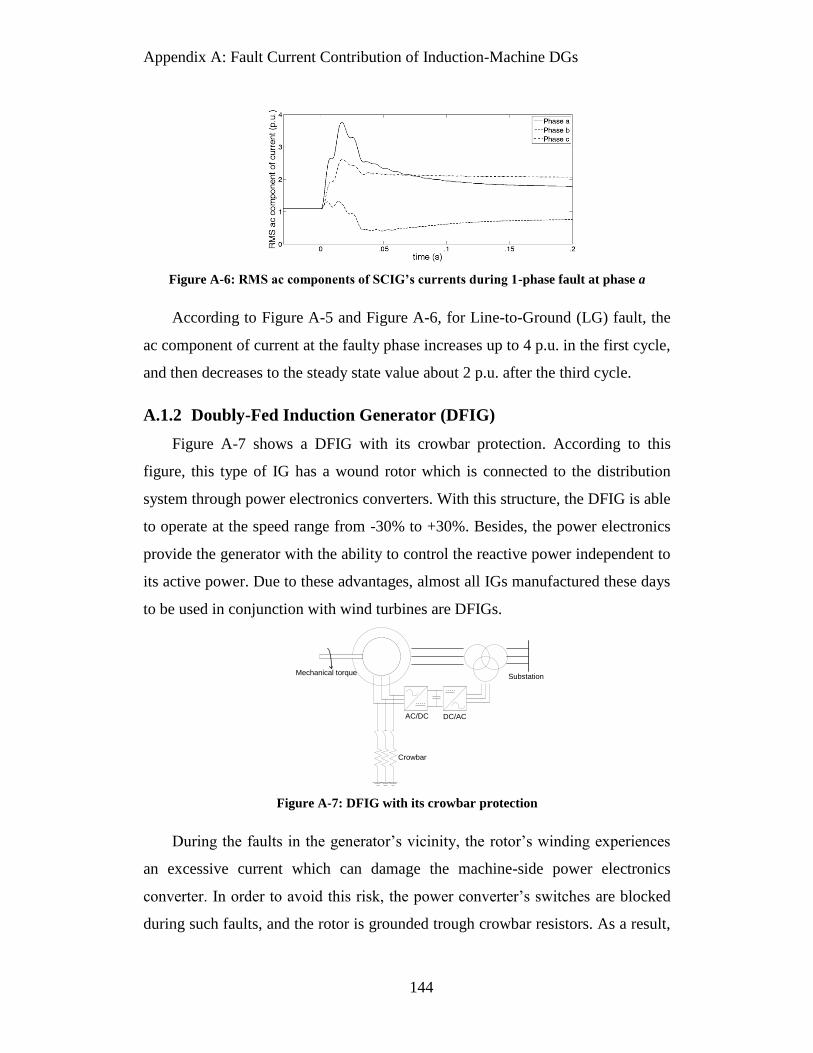
Appendix A: Fault Current Contribution of Induction-Machine DGs
144
Figure A-6: RMS ac components of SCIG’s currents during 1-phase fault at phase a
According to Figure A-5 and Figure A-6, for Line-to-Ground (LG) fault, the
ac component of current at the faulty phase increases up to 4 p.u. in the first cycle,
and then decreases to the steady state value about 2 p.u. after the third cycle.
A.1.2 Doubly-Fed Induction Generator (DFIG)
Figure A-7 shows a DFIG with its crowbar protection. According to this
figure, this type of IG has a wound rotor which is connected to the distribution
system through power electronics converters. With this structure, the DFIG is able
to operate at the speed range from -30% to +30%. Besides, the power electronics
provide the generator with the ability to control the reactive power independent to
its active power. Due to these advantages, almost all IGs manufactured these days
to be used in conjunction with wind turbines are DFIGs.
Mechanical torque
AC/DC
Substation
DC/AC
Crowbar
Figure A-7: DFIG with its crowbar protection
During the faults in the generator’s vicinity, the rotor’s winding experiences
an excessive current which can damage the machine-side power electronics
converter. In order to avoid this risk, the power converter’s switches are blocked
during such faults, and the rotor is grounded trough crowbar resistors. As a result,

Appendix A: Fault Current Contribution of Induction-Machine DGs
145
the DFIG’s behaviour during the fault is completely similar to the SFIG’s
behaviour with large external rotor resistance. The Simulation results confirm this
idea. Figure A-8 and Figure A-9 the RMS ac component of the DFIG’s current
during a 3-phase fault at its terminals for slips of +20% and -20%, respectively.
Comparison between these figures and Figure A-4 shows that regardless of
operating slip, DFIG’s response to fault is similar to the wound rotor SFIG’s
response when it operates at a relatively high slip (high rotor resistance).
Figure A-8: RMS ac component of DFIG’s current during 3-phase fault at its terminals
(Slip=+20%)
Figure A-9: RMS ac component of DFIG’s current during 3-phase fault at its terminals
(Slip=-20%)
In order to achieve a general conclusion about contribution of DFIGs to 3-
phase fault currents, Table A-2 has been re-generated under the assumption that
IGs are DFIG this time, and the crowbar resistance is twice the rotor’s resistance.
As this table reveals, contribution of all the generators to the fault current at the
third cycle is less than .7 p.u., and in the 5th
cycle, they have almost no
contribution to the fault current. Also, the comparison between Table A-2 and
Table A-3 shows that the crowbar operation highly accelerates the damping of
generator’s current during the fault.

Appendix A: Fault Current Contribution of Induction-Machine DGs
146
Table A-3: Electrical circuit parameters of commercially available IGs [4] and their
contribution to 3-phase fault at terminals when considered as DFIG
No. Manufacturer P
(MW)
Rs
(p.u.)
Xs
(p.u.)
Rr
(p.u.)
Xr
(p.u.)
Xm
(p.u.)
If
(p.u.)
3rd
cycle
If
(p.u.)
5th
cycle
1 Nordex 1 0.0062 0.0787 0.0092 0.0547 3.642 0.14 0.01
2 Negmicon 1.5 0.0227 0.0795 0.0156 0.0597 3.755 0.01 0.00
3 Negmicon 1 0.0225 0.173 0.008 0.13 3.428 0.66 0.24
4 WindWorld 0.6 0.0197 0.1271 0.0089 0.0956 4.667 0.44 0.1
5 Bonus 0.6 0.0065 0.0894 0.0093 0.1106 3.887 0.34 0.06
6 Bonus 1 0.0062 0.1362 0.0074 0.1123 3.911 0.69 0.224
7 Vestas 1.66 0.0077 0.0697 0.0062 0.0834 3.454 0.63 0.14
A.2 Findings from an experimental research work
In this sub-section, the results of experimental short circuit tests on an IG are
provided to confirm the results achieved in previous sub-sections. In [6], 3-phase
short circuit tests were performed at the terminals of a 415 V 7.5 kW IG in both
SFIG and DFIG modes. Figure A-10 and Figure A-11 show the responses of
SFIG and DFIG to the fault, respectively [6].
Figure A-10: SFIG’s 3-phase current during an experimental 3-phase fault at its terminals
[6]

Appendix A: Fault Current Contribution of Induction-Machine DGs
147
Figure A-11: DFIG’s 3-phase current during an experimental 3-phase fault at its terminals
[6]
As Figure A-10 reveals, SFIG’s current reaches up to 4 p.u. in the first cycle
after the beginning of fault. However, it decreases quickly so that in the third
cycle it is less than 1 p.u. On the other hand, for DFIG (Figure A-11) the current
decreases below 1 p.u. in the second cycle after the fault, and in the third cycle, it
is almost zero. These results show agreement with the analytical and simulated
results. The slight difference is that the simulated waveforms have higher peaks
and are smoother than experimental waveforms which is due to neglecting
magnetic saturation in simulations.
From the mathematical analysis, simulation and experimental results
provided in sub-sections 4.1 and 4.2 it can be concluded that SFIG with no
external rotor resistance has the highest peak of fault current and the longest
transient time constant (slowest damping and widest contribution time window) in
comparison to other IGs. Consequently, in the next section, SFIG is used to
determine the impact of IG on the O.C. protection coordination.
A.3 Impact on the protection coordination
In this section, contribution of SFIG, as the worst case, to phase-to-phase and
phase-to-ground faults in the distribution system is studied and its impact on the
O.C. protection is analyzed. To do so, the sample 25 kV distribution system
shown in Figure 4-5 was simulated again. This time, the SMDG was replaced by
the SFIG with the parameters tabulated in Table A-1. The protection system and
its settings are similar to those presented in 4.3.1.

Appendix A: Fault Current Contribution of Induction-Machine DGs
148
A.3.1 Phase-to-phase faults
Similar to the SMDG of the case study presented in 4.3.1, when a SFIG is
added upstream of B2, it is suspected to contribute to the fault and increase the
fault current which flows through the protection devices. This increase may cause
miscoordination between B1 and B2. As an example, consider a fault at F3. When
there is no DG, the current through B2 is 4187A which leads to the operation of
its short-time delay element, while the current through B1 is 4190A which results
in operation of its inverse-time relay. However, when the SFIG is embedded, if it
increases the fault current at F3 above 4440A (pick-up current of B1’s
instantaneous relay), both B1 and B2 will operate simultaneously, and the whole
feeder is de-energized.
In order to examine the possibility of such miscoordination, a 9MW SFIG
(90% of total load on the feeder) was embedded upstream of B2 (arbitrarily at the
substation S) and its contribution to different phase-to-phase faults at F3 were
determined. Figure A-12 shows the effect of the SFIG on the 3-phase fault
current, and Figure A- 13 shows its effect on the phase a to phase b fault current.
Figure A-12: Impact of 9MW SCIG on 3-phase fault current
Figure A- 13: Impact of 9MW SCIG on phase a-to-phase b fault current

Appendix A: Fault Current Contribution of Induction-Machine DGs
149
As both figures illustrate, the fault current decreases below the coordination
boundary in less than .05 sec. which means that the coordination maintains in both
cases, and the SFIG has no impact on the coordination. It is due to fast damping
of the SFIG’s fault current. However, in this case, the SFIG can cause
miscoordination at higher capacities, or if the short-time delay elements’
operation time are set below .05 sec.
A.3.2 Phase-to-ground faults
Table A-4 shows the LG fault current at F3 for different scenarios, and its
increment due to the insertion of 9MW SFIG. According to this table, in most
cases, in contrast to what was expected, the SFIG decreased the single phase to
ground fault few percent. Only in four scenarios in which substation transformer
(Ts) at low voltage side has Yg connection, the SFIG has positive contribution to
fault, and its maximum contribution is 6.7%.
Table A-4: Contribution of SCIG to LG fault
Ts
Fault
current (A)
(No DG)
Fault current
(A)
(9MW IG,
TIG: DYg)
Incremental
current due to IG
(%)
Fault
current (A)
(9MW IG,
TIG: YgYg)
Incremental
current due to
IG (%)
YY 678 665 -1.92 667 -1.62
YD 678 665 -1.92 667 -1.62
YYg 693 676 -2.45 678 -2.16
DY 678 665 -1.92 667 -1.62
DD 678 665 -1.92 667 -1.62
DYg 5528 5900 6.73 5753 4.07
YgYg 3973 4153 4.53 4082 2.74
YgY 678 665 -1.92 666 -1.77
YgD 678 665 -1.92 667 -1.62
In order to investigate the impact of the SFIG on the coordination consider
the worst condition in which it has 6.7% contribution, and imagine that B1 and B2
are equipped with inverse O.C. relays (with IEC 60255 characteristic equation)
for ground fault protection with the settings tabulated in Table A-5. In this case,
when there is no DG, for phase-to-ground fault at F3, B2 operates at .073 sec. and

Appendix A: Fault Current Contribution of Induction-Machine DGs
150
B1 operates at .32 sec., and there is a .25 sec. interval between main and back-up
protection devices’ operation. When a 9MW SCIG is embedded at substation, the
ground fault current is increased from 5528A to 5900A. In this case, B2 as the
main protection operates at .0728 and B1 as the back-up operates at .319 sec, and
still there is a .246 sec. interval between the main and back-up protection, and the
coordination maintains.
Table A-5: ground fault relays’ settings
Ipick-up (A) TSM
B1 80 .05
B2 60 .2
A.4 Conclusion
In this section, the contribution of IMDGs to the fault current was studied,
and their impact on the O.C. protection coordination was investigated. The results
are summarized as follows:
1. In the first cycle after the beginning of symmetrical faults, IG’s
current reaches to 6p.u. However, it decreases to zero in the next
cycles. During asymmetrical faults, the IG’s output current is higher
than its rated current with a peak up to 4 p.u. in the first three cycles
and the steady state value of 2 p.u. in the next cycles.
2. Due to the short contribution time window in case of phase-to-phase
faults, the IG has no impact on O.C. coordination unless there are
instantaneous or short-time delay elements with the operation time
less than .05 sec. (three cycles) in the protection system, and the IG
penetration level is so high, which is not common.
3. In case of phase-to-ground faults, simulations showed that the
maximum contribution of the SFIG at very high penetration levels is
limited to 7% of original fault current which is not sufficient to cause
miscoordination between the main and back-up inverse O.C. ground
fault relays.

Appendix A: Fault Current Contribution of Induction-Machine DGs
151
4. Due to their advantages, DFIGs become more and more popular, and
almost all IGs being installed in the wind plants these days are DFIGs.
Besides, it was shown that, due to crowbar protection, DFIG’s
contribution to the fault current is negligible. So, one can say that
embedding IGs in the distribution system is not a concern from the
protection coordination point of view.

Appendix B: Fault Current Contribution of Permanent Magnet Synchronous
Generators
152
Appendix B:
Fault Current Contribution of
Permanent Magnet Synchronous
Generators
Permanent Magnet Synchronous Generators (PMSGs) have been used in
three DG applications: wind turbines with full-scale converters, micro-turbines
and micro hydro power plants. In the first two applications, PMSG is connected to
the grid through an inverter. Consequently, DG’s contribution to the grid faults
depends on its inverter’s control and protection (see Section 3) rather than the
PMSG’s parameters. In contrast, in the third application, PMSG is directly
connected to the grid and directly responds to the grid faults. The main aim of this
section is to investigate the response of the direct-connected PMSG to the fault
and compare its contribution to fault current with the contribution of regular
WFSG which was studied in previous section.
In following paragraphs, an analytical method to calculate PMSG’s fault
current is presented. Next, comparison between WFSG’s and PMSG’s responses
to faults is presented. Then, a method to estimate the PMSG’s contribution to
faults for O.C. coordination studies is provided which is followed by the
conclusion.

Appendix B: Fault Current Contribution of Permanent Magnet Synchronous
Generators
153
B.1 PMSG’s fault current
Figure B-1 shows the equivalent 0dq circuit of a PM synchronous
machine [7]. As this figure reveals, PM is modeled as a d-axis
magnetization current (im).
ωψdrs Lls
Lmq
Llkq rkq ikqiq
rs Llsi0
ωψqrs Lls
Lmd
Llkd
rkdikd
id
im
vd
vq
v0
Figure B-1: Equivalent 0dq circuit of a PM synchronous machine
According to Figure B-1 0dq voltage equations can be written as follows [7]:
00 0
q
q s q d
dd s d q
s
dv r i
dt
dv r i
dt
dv r i
dt
(B- 1)
where
0 0
q q q mq kq
d d d md kd md m
ls
L i L i
L i L i L i
L i
(B- 2)
and

Appendix B: Fault Current Contribution of Permanent Magnet Synchronous
Generators
154
q mq ls
d md ls
L L L
L L L
(B- 3)
During a three-phase solid fault at machine’s terminal, current can be
obtained by equating 0dq voltages with zero. Then, by transforming 0dq currents,
abc currents are obtained. By doing so, AC fundamental component of PMSG’s
current at phase a can be determined as follows:
""
0 0" "
1 1 1 1 1 1cos( ) sin( )qd
tt
TT
a mq md
d d d q q q
i U e t U e tX X X X X X
(B- 4)
where θ0 is the angle between the field and phase a coils’ axis at the fault instance
and:
" md kdd ls
md kd
X XX X
X X
(B- 5)
" mq kq
q ls
mq kq
X XX X
X X
" 1( )md ls
d kd
kd md ls
X XT X
r X X
" 1( )md ls
q kq
kq md ls
X XT X
r X X
As (B- 4) reveals, PMSG’s response can be divided into two periods: sub-
transient and steady state.
B.2 Comparison of PMSG’s and WFSG’s fault currents
The first and most important difference between PMSG and WFSG is that in
the first one the magnetic field is provided by PMs, while in the latter one the
magnetic field is provided by a field winding. As a result, an additional time
constant T’d and an additional operational reactance X’d appear in the WFSG’s
response to fault (see (B- 6)).

Appendix B: Fault Current Contribution of Permanent Magnet Synchronous
Generators
155
' "
"
0' " '
0"
1 1 1 1 1cos( )
1 1 1sin( )
d d
q
t t
T T
a mq
d d d d d
t
T
md
q q q
i U e e tX X X X X
U e tX X X
(B- 6)
Comparison between (B- 4) and (B- 6) reveals that the WFSG’s response to
fault is divided into three periods (instead of two) which are: sub-transient,
transient and steady state.
The second difference is that the sub-transient time constant of PMSG could
be so short that after one or two cycles, PMSG’s fault current reaches its steady
state [8]. Moreover, operational reactances of PMSG are typically smaller than the
operational reactances of WFSG. In summary:
" " '
, , , , ,d PMSG d WFSG d WFSG d PMSG d WFSGX X X X X (B- 7)
" "
, , , ,q PMSG q WFSG q PMSG q WFSGX X X X
(B- 8)
" " '
, , ,d PMSG d WFSG d WFSGT T T
(B- 9)
" "
, ,q PMSG q WFSGT T
(B- 10)
Typical time constants and operational reactances for PMSG and WFSG are
collected and tabulated in Table B-1 [8]-[10]:
Table B-1: Typical time constants and reactances of synchronous generators [8]-[10]
Parameter Typical value for
PMSG
Typical value for
WFSG
Xd 0.45 (p.u.) 1.2 (p.u.)
Xd' - 0.35 (p.u.)
Xd" 0.13 (p.u.) 0.25 (p.u.)
Xq 0.45 (p.u.) 0.9 (p.u.)
Xq" 0.13 (p.u.) 0.28 (p.u.)
Td' - 1.4 sec.
Td" 8 m.sec. 160 m.sec.
Tq" 8 m.sec. 160 m.sec.

Appendix B: Fault Current Contribution of Permanent Magnet Synchronous
Generators
156
According to (B- 4), (B- 6) and Table B-1, for generators with the same size,
PMSG has higher output than WFSG in the first one or two cycles after the fault
(sub-transient response). Next, PMSG’s current decrease to its steady-state value,
while WFSG’s current starts its transient period. Since Xd,WFSG'<Xd,PMSG, for
several cycles WFSG’s current is higher than PMSG’s current. Finally, WFSG
also reaches its steady state, and because Xd,PMSG< Xd,WFSG, it has lower output
current than PMSG’s current. For further illustration, one PMSG and one WFSG
were simulated in Matlab/Simulink with the parameters tabulated in Table B-1.
Figure B-2 shows the output currents of these machines during a three-phase solid
fault at terminals, and Figure B-3 shows the RMS ac component of these currents.
Figure B-2: Current at phase a for three-phase solid fault at terminals
Figure B-3: RMS ac component of current at phase a for three-phase solid fault at terminals
As Figure B-3 demonstrates, during the first two cycles, fault current of
PMSG is higher than that of the WFSG. Next, after the second cycle, sub-
transient responses of generators disappeared, and PMSG’s current reached its
steady-state value around 2.5 p.u. while transient response of WFSG started with
almost 4 p.u. which gradually decreased.
0 .05 .1 .15 .2-4
-2
0
2
4
6
8
time (s)
Outp
ut curr
ent (A
)
WFSG
PMSG
0 .05 .1 .15 .2 .25 .3
1
2
3
4
5
6
time (s)
RM
S a
c c
urr
ent (p
.u.)
WFSG
PMSG

Appendix B: Fault Current Contribution of Permanent Magnet Synchronous
Generators
157
B.3 Estimation of PMSG’s contribution to fault
As Figure 2-3 revealed in Chapter 2, almost all O.C. devices operate after
0.03 sec. (2 cycles after the beginning of fault). Besides, in previous section it was
shown that PMSG’s sub-transient response disappears in two cycles. As a result,
for O.C. coordination studies in distribution system, sub-transient part of
machine’s response can be neglected. In this case, PMSG’s current can be
estimated as:
0 0
1 1cos( ) sin( )a mq md
d q
i U t U tX X
(B- 11)
The RMS value of (B- 11) is as follows:
22
,
mq mda RMS
d q
U Ui
X X
(B- 12)
Now, by neglecting machine’s saliency, (B- 12) could be simplified as:
2 2
,
1a RMS mq md
d d
Ui U U
X X (B- 13)
where U is the machine’s no-load voltage, and can be estimated as follows (by
assuming rated output current at unity power factor during pre-fault and
neglecting stator resistance and rotor saliency):
21 dU X (B- 14)
Now, from (B- 13) and (B- 14):
2
,
11 ( )a RMS
d
iX
(B- 15)
From (B- 15), RMS ac component of current for the PMSG simulated in
previous part is obtained as 2.437 p.u. which is close to the simulation result
2.484 p.u.
In order to compare the impact of PMSG and WFSG on the O.C.
coordination, it is necessary to consider the O.C. devices’ operation time frames.
From Table B-1 and Figure 2-3 it can be concluded that the operation of the O.C.

Appendix B: Fault Current Contribution of Permanent Magnet Synchronous
Generators
158
devices normally coincides with the transient response of WFSG. This part of
WFSG’s response has a decaying trend and can be estimated as follows:
'
, '
1 1 1d
t
T
a RMS
d d d
i U eX X X
(B- 16)
As a result (B- 16) should be compared with (B- 13).
If inverse and/or very inverse O.C. devices are involved in the protection
(t>.3), it is hard to compare (B- 13) and (B- 16). However, Figure B-3 reveals that
in this period, the contribution of PMSG and WFSG are almost the same.
If extremely inverse or short-time delay elements are involved in the
coordination (scenarios in which miscoordination is more likely to happen),
'
1d
t
Te
and consequently for WFSG:
, 'a RMS
d
Ui
X (B- 17)
where U can be estimated by (B- 14). As a result:
2 ',, ,
2, ,,
1
1
d PMSGRMS PMSG d WFSG
RMS WFSG d PMSGd WFSG
Xi X
i XX
(B- 18)
Now, by inserting typical values from Table 1, in such time frame
,
,
0.6RMS PMSG
RMS WFSG
i
i . In other words, the contribution of PMSG is 60% of the
contribution of WFSG with the same size.
B.4 Limiting PMSG’s fault current
In previous sections, it was shown that the PMSG’s response to fault can be
divided into two periods. The sub-transient response is too quick to impact the
O.C. coordination. As a result, this part focuses on limiting the steady state
response of PMSG.

Appendix B: Fault Current Contribution of Permanent Magnet Synchronous
Generators
159
By substituting (B- 19) and (B- 20) in (B- 17), it is shown that the ac
component of PMSG’s current is equal to the ratio of its d-axis flux to its
inductance.
dU (B- 19)
d dX L
(B- 20)
,d
a RMS
d
iL
(B- 21)
As (B- 21) reveals, a large inductance can restrict PMSG’s current during a
fault. So, one way to limit PMSG’s current is to consider a large Ld for machine,
during design procedure. Another way is weakening its flux during the fault. Flux
adjustment requires an additional mechanism to be implemented in the machine.
This mechanism could be either utilizing an auxiliary field winding or a
mechanical mechanism. These machine’s fault current limiting streams are
reviewed in the following sections.
B.4.1 PM machines with large leakage inductance
The idea of designing PM machines with large inductance has been proposed
and used in designing fault-tolerant machines. These machines should meet
specific requirements such as high power density and high reliability to be
appropriate for aerospace and automotive applications [11]-[14]. In fault-tolerant
PM machines, using PM ensures high power density. Besides, fault current should
be limited to the rated current to prevent machine’s damage during the short
circuit which is a reliability requirement.
In [15],[16] the PM machine’s short circuit current has been calculated as
follows:
( ) sin( )a sc
sc
i t tZ
(B- 22)

Appendix B: Fault Current Contribution of Permanent Magnet Synchronous
Generators
160
Where ( )scsin t - is the back EMF due to the PM flux
linkage , and √ is the phase impedance. Since in practice
<< , magnitude of fault current can be estimated as follows:
,a RMSiL
(B- 23)
which is consistent with the result achieved in previous section. Based on (B- 23),
[11]-[24] have concluded that a fault tolerant machine should be designed so that
its per-unit inductance is equal to its per-unit flux linkage. In addition, mutual
inductance between phases should be negligible to avoid fault propagation [11].
So, this large inductance is mainly leakage inductance.
Although it may sound difficult to achieve a PM machine design which
provides large leakage inductance, in [13] it has been shown that even for small
PM machines large leakage inductance is easily achievable. According to [17], the
desired leakage inductance can be gained by controlling depth and width of slot
opening.
Nevertheless, such design associates with a major disadvantage which is
increase in machine’s flux that requires wider stator teeth [13]. Additional tooth
width and deeper reactance slots can increase machine weight by 15% [19].
B.4.2 PM machines with auxiliary excitation
One way to control the PMSG’s flux is to add an auxiliary field winding with
adjustable supply to regulate the total air-gap flux. These PM machines with
additional field windings are called Hybrid Excitation Synchronous Machines
(HESMs). In following paragraphs, HESMs are divided into two categories, based
on the location of auxiliary winding, and advantages and disadvantages of them
are reviewed.
a. PM machines with auxiliary excitation on the rotor
This category includes the PMSGs with auxiliary field winding mounted on
their rotors. Figure B-4 shows a simple example of this type. As it can be seen in

Appendix B: Fault Current Contribution of Permanent Magnet Synchronous
Generators
161
this figure, rotor is separated to two independent parts, PM and wound field [25].
Each part of the rotor induces a back EMF, and depending on the direction of
field current, these two EMFs can either boost or cancel each other.
Figure B-4: HESM with separated rotors on the same shaft [21]
There are also other types of HESMs in which rotor is not separated to two
distinguished parts, i.e. both field winding and PMs are mounted on the same
rotor part. These machines have more complicated rotor structures, and depending
on the path of the flux generated by the auxiliary winding, they are classified into
two subcategories [22]:
Series flux path
Parallel flux path
In HESMs with series flux path, the flux generated by auxiliary winding
passes through PMs. Series flux HESMs have simpler structure than parallel ones,
and good flux weakening capability up to 50% [22]. However, there is a risk for
irreversible demagnetization [23].
On the other hand, in HESMs with parallel flux path, the flux generated by
PM and the one generated by auxiliary field winding have different paths. In
contrast to series flux path HESMs, there is a wide variety of structures for these
machines [23]. However, these structures are more complicated than series ones
either for analysis or for manufacturing [22].
Regardless of being series or parallel flux path, HESMs with field winding on
the rotor, has a major drawback. These machines require brushes and slip rings or
rotary diodes to supply the auxiliary winding mounted on rotor.

Appendix B: Fault Current Contribution of Permanent Magnet Synchronous
Generators
162
b. PM machines with auxiliary excitation on the stator
This category includes machines in which PMs are mounted on the rotor,
while the auxiliary field winding is embedded in the stator. Major advantage of
such design is that these machines do not require brushes and slip rings.
Nevertheless, both rotor and stator structures are complicated in these machines.
Figure B-5 shows the structure of the consequent-pole PM machine proposed
in [26]. As it can be seen, rotor includes both iron poles and magnets. Besides,
stator is divided into two parts, and a circumferential DC field winding is
embedded between these two parts. The flux provided by PMs combines with the
flux provided by auxiliary winding in the air-gap. Depending on the direction of
excitation current, flux generated by winding can boost or weaken the PM flux.
There is no risk of demagnetization, and low Amp-turn is required for air-gap flux
control [26]. However, complicated structure causes manufacturing problems
[26].
Figure B-5: Consequent-pole permanent magnet machine [26]
Regardless of the location of auxiliary winding, all HESMs suffer from the
following disadvantages:
Embedding an auxiliary field winding increases machine’s weight, and
hence, decreases machine’s power density.
An independent power source and converter are needed to supply DC
field.
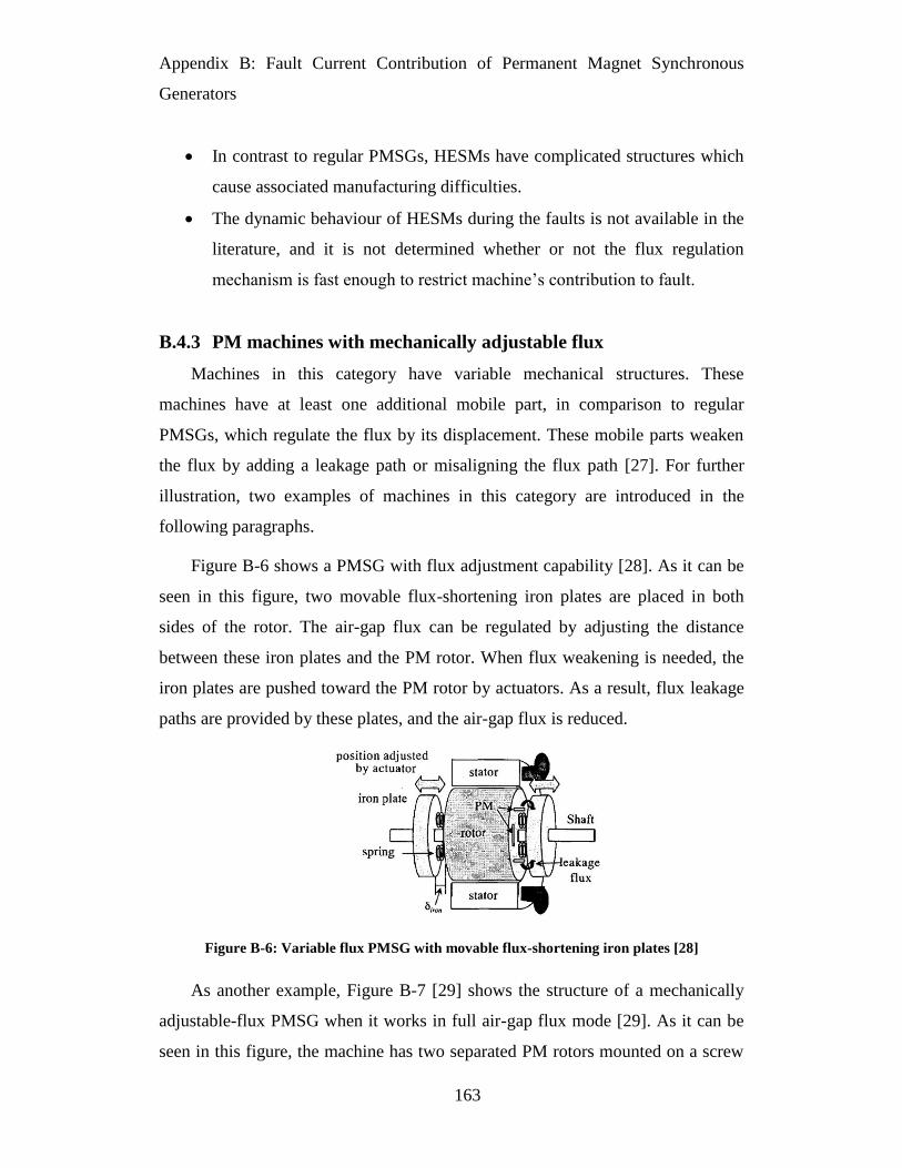
Appendix B: Fault Current Contribution of Permanent Magnet Synchronous
Generators
163
In contrast to regular PMSGs, HESMs have complicated structures which
cause associated manufacturing difficulties.
The dynamic behaviour of HESMs during the faults is not available in the
literature, and it is not determined whether or not the flux regulation
mechanism is fast enough to restrict machine’s contribution to fault.
B.4.3 PM machines with mechanically adjustable flux
Machines in this category have variable mechanical structures. These
machines have at least one additional mobile part, in comparison to regular
PMSGs, which regulate the flux by its displacement. These mobile parts weaken
the flux by adding a leakage path or misaligning the flux path [27]. For further
illustration, two examples of machines in this category are introduced in the
following paragraphs.
Figure B-6 shows a PMSG with flux adjustment capability [28]. As it can be
seen in this figure, two movable flux-shortening iron plates are placed in both
sides of the rotor. The air-gap flux can be regulated by adjusting the distance
between these iron plates and the PM rotor. When flux weakening is needed, the
iron plates are pushed toward the PM rotor by actuators. As a result, flux leakage
paths are provided by these plates, and the air-gap flux is reduced.
Figure B-6: Variable flux PMSG with movable flux-shortening iron plates [28]
As another example, Figure B-7 [29] shows the structure of a mechanically
adjustable-flux PMSG when it works in full air-gap flux mode [29]. As it can be
seen in this figure, the machine has two separated PM rotors mounted on a screw

Appendix B: Fault Current Contribution of Permanent Magnet Synchronous
Generators
164
thread shaft. One of these rotor parts can be misaligned by an actuator. In this
case, less flux linkage is experienced by the stator. Figure B-8 shows this machine
when the air-gap flux is nullified [29].
Figure B-7: Variable flux PMSG with two rotors on a screw thread shaft in maximum air-
gap flux operation mode [29]
Figure B-8: Variable flux PMSG with two rotors on a screw thread shaft in nullified air-gap
flux operation mode [29]
Regardless of the adjusting mechanism, mechanically adjustable-flux PMSGs
suffer from the following disadvantages:
These machines usually have more complicated structures than regular
PMSGs.
Due to the fact that the flux adjustment requires displacement of
mechanical parts, these machines have relatively long response time.
Actuators and other additional parts require maintenance, and lower the
machine’s reliability.

Appendix B: Fault Current Contribution of Permanent Magnet Synchronous
Generators
165
B.5 Conclusion
The PMSG’s response during the fault and its contribution to the fault current
were studied in this section. It was shown that:
1. The response of these machines to fault is divided into two periods:
sub-transient which disappears after the second cycle of fault, and the
steady state which coincides with the operation of O.C. devices.
2. In the first two cycles after the fault, PMSG has higher contribution
than WFSG. Next, PMSG starts its steady-state response. In this
period, which coincides with the typical operation interval of O.C.
devices, the contribution of PMSG is lower than the contribution
WFSG at the same size.
3. PMSG’s are relatively small machines with the contribution up to
250% their rated current. This contribution is remarkably less than the
contribution of WFSGs in scenarios where miscoordination is more
likely to happen. As a result, PMSGs may not be a concern for O.C.
protection coordination.
4. Amongst all the PMSG’s fault current limiting methods, is the most
suitable one, due to the following reasons:
It does not require actuator or brushes and slip rings. So, it
does not impact the machine’s reliability and does not
demand for additional maintenance.
Limited fault current is an inherent property in machines with
enlarged leakage reactance, and it does not need fault
detection and trigger mechanisms and is not affected by
response time, delay, etc.
Enlarging PMSG’s leakage reactance can be achieved by
choosing suitable values for machine design parameters and it
does not need complicated rotor and stator structures.

Appendix B: Fault Current Contribution of Permanent Magnet Synchronous
Generators
166
This method does not need additional power source/converter
to supply auxiliary winding or actuators.
The only penalty of large PMSG’s leakage reactance is an
increase in machine’s weight up to 15%.

167
References of Appendices
[1] E. Muljadi, N. Samaan, V. Gevorgian, J. Li and S. Pasupulati, “Short Circuit
Current Contribution for Different Wind Turbine Generator Types,” IEEE
Power and Energy Society General Meeting, 2010, pp. 1–8.
[2] W. Freitas, C. M. Vieira, A. Morelato, L. C. P. da Silva, V. F. da Costa and
F. A. B. Lemos, “Comparative Analysis Between Synchronous and
Induction Machines for Distributed Generation Application,” IEEE Trans.
Power System, vol. 21, no. 1, pp 301-311, February 2006.
[3] J. Morren and S. W. H. de Haan, “Short-Circuit current of Wind Turbines
With Doubly Fed Induction Generator,” IEEE Trans. Energy Conversion,
vol. 22, no. 1, pp 174-180, March 2007.
[4] A. G. G. Rodrigez, “Improvement of Fixed-Speed Wind Turbine Soft Starter
Based On A Sliding Mode Controller,” PhD Dissertation, Dept. Elect. Eng.,
Univ. of Seville, Seville, Spain, March 2006.
[5] J. Lopez, E. Gubia, P. Sanchis, X. Roboam and L. Marroyo, “Wind Turbines
Based on Doubly Fed Induction Generator Under Asymmetrical Voltage
Dips,” IEEE Trans. Energy Conversion, vol. 23, no. 1, pp 321-329, March
2008.
[6] G. Pannell, D. J. Atkinson and B. Zahawi, “Analytical Study of Grid-Fault
Response of Wind Turbine Doubly Fed induction Generator,” IEEE Trans.
Energy Conversion, vol. 25, no. 4, pp 1081-1091, December 2010.
[7] C. Ong, Dynamic Simulation of Electric Machinery Using Matlab/Simulink,
Upper Saddle River, NJ Prentice Hall, 1998
[8] K. W. Klontz, T. J. E. Miller, M. I. McGlip, H. Karmaker, and P. Zhong,
“Short-Circuit Analysis of Permanent-Magnet Generators,” IEEE Trans.
Industry Applications, vol. 47, no. 4, pp 1670-1680, 2011.
[9] Test Procedures for Synchronous Machines IEEE Standard 115, 1994
[10] E. W. Kimbark, Power System Stability, Piscataway, NJ: IEEE Press,1995

168
[11] N. Bianchi, S. Bolognani, and M. Dai Pre, “Design and tests of a fault-
tolerant five-phase permanent magnet motor,” in Proc. IEEE Power
Electron. Spec. Conf., Jun. 2006, pp. 1–8.
[12] N. Bianchi and S. Bolognani, “Strategies for the Fault-Tolerant Current
Control of a Five-Phase Permanent-Magnet Motor,” IEEE Trans. Industry
Applications, vol. 43, no. 4, pp 960-971, 2007.
[13] B. C. Mecrow, A. G. jack, J. A. Haylock and J. Coles, “Fault-tolerant
permanent magnet machine drives,” IEE Proc.-Electr. Power Appl., Vol.
143, No. 6, pp. 431-436, November 1996.
[14] T. Raminosoa and C. Gerada, “A comparative study of permanent magnet -
synchronous and permanent magnet - flux switching machines for fault
tolerant drive systems,” IEEE Energy Conversion Congress and Exposition,
12-16 Sept. 2010, pp. 2471-2478.
[15] C. Bianchini, E. Fornasiero, T. N. Matzen, N. Bianchi, and A. Bellini, “Fault
detection of a five-phase permanent-magnet machine,” in Proc. 34th Annu.
IEEE IECON, 2008, pp. 1200–1205.
[16] J. Chai, J. Wang, K. Atallah, and D. Howe, “Performance comparison and
winding fault detection of duplex 2-phase and 3-phase fault-tolerant
permanent magnet brushless machines,” in Conf. Rec. IEEE IAS Annu.
Meeting, Sydney, Austrailia, Sep. 2007, pp. 566–572.
[17] B.C. Mecrow, A. G. Jack, D. J. Atkinson, S. Green and G. J. Atkinson,
“Design and Testing of a 4 Phase Fault Tolerant Permanent Magnet
Machine for an Engine Fuel Pump”, Electric Machines & Drives Conf., Vol.
2, June 2003, pp. 1301–1302.
[18] N. Bianchi and M. Dai Prè, “Use of the star of slots in designing fractional-
slot single-layer synchronous motors,” Proc. Inst. Elect. Eng.—Elect. Power
Appl., vol. 153, no. 3, pp. 459–466, May 2006.

169
[19] J. A. Haylock, B.C. Mecrow, A. G. Jack and D. J. Atkinson, “Operation of
fault tolerant machines with winding failures,” in Proc. IEEE Int. Electr.
Mach. and Drives Conf., 1997, pp. MC3/10.1–MC3/10.3.
[20] B. Welchko, T. Jahns, W. Soong, and J. Nagashima, “Ipm synchronous
machine drive response to symmetrical and asymmetrical short circuit
faults,” IEEE Transactions on Energy Conversion, vol. EC–18, Jun. 2003.
[21] N. Naoe and T. Fukami, “Trial production of a hybrid excitation type
synchronous machine,” in Conf. Rec. IEEE-IEMDC, Cambridge, MA, Jun.
17–20, 2001, pp. 545–547.
[22] R. Owen, Z.Q. Zhu, J.B. Wang, D. A. Stone, and I. Urquhart, “Review of
variable-flux permanent magnet machines,” Int. Conf. on Elec. Machines
and Systems, 20-23 August, 2011, Beijing.
[23] Y. Amara, L. Vido, M. Gabsi, E. Hoang, A. H. Ben Hamed, and M.
Lécrivain, “Hybrid excitation synchronous machines: Energy-efficient
solution for vehicles propulsion,” IEEE Trans. Veh. Technol., vol. 58, no. 5,
pp. 2137–2149, Jun. 2009.
[24] G. Henneberger, J. R. Hadji-Minaglou, and R. C. Ciorba, “Design and test
of permanent magnet synchronous motor with auxiliary excitation winding
for electric vehicle application,” in Proc. Eur. Power Electron. Chapter
Symp., Lausanne, Switzerland, Oct. 1994, pp. 645–649.
[25] D. Fodorean, A. Djerdir, I. A. Viorel, and A. Miraoui, “A double excited
synchronous machine for direct drive application—Design and prototype
tests,” IEEE Trans. Energy Convers., vol. 22, no. 3, pp. 656–665, Sep. 2007.
[26] J. A. Tapia, F. Leonardi, and T. A. Lipo, “Consequent-pole
permanentmagnet machine with extended field-weakening capability,” IEEE
Trans. on Industry Applications, vol. 39, No 6, pp. 1704-1709, Nov./Dec.
2003.

170
[27] A. D. Akemakou and S. K. Phounsombat, “Electrical machine with double
excitation, especially a motor vehicle alternator,” U.S. Patent 6 147 429,
Nov. 14, 2000.
[28] H. Wang, Y. Wang, X. Liu, G. Cao and J. Fan, “Design and Performance
Evaluation of Compound Permanent Magnet Generator With Controllable
Air-gap Flux,” IET Electr. Power Appl., 2011, Vol. 5, Iss. 9, pp. 684–690
[29] L. Ma, M. Sanada, S. Morimoto, & Y. Takeda, “Advantages of IPMSM with
adjustable PM armature flux linkage in efficiency improvement and
operating range extension,” Proceedings of the Power Conversion
Conference, 2002. PCC Osaka 2002, vol.1, pp.136-141, 2002
Recommended