UNIVERSITY OF NAIROBI
PROJECT CODE: PMO 01/2015
PROJECT TITLE: DETERMINATION OF THE AMOUNT OF ENERGY
RECOVERABLE FROM A FLUE GAS STREAM IN A COMMERCIAL
INCINERATOR
PROJECT SUPERVISOR: DR. PHILIP MWABE
PROJECT UNDERTAKEN BY:-
KAIMBA BRENCIL GISLOP F18/1427/2010
MAINA TITUS GITHIGIA F18/1429/2010
A FINAL YEAR PROJECT FOR THE PARTIAL FULLFILMENT FOR THE AWARD
OF BACHELORS DEGREE IN MECHANICAL AND MANUFACTURING
ENGINEERING OF THE UNIVERSITY OF NAIROBI
APRIL 2015
DEPARTMENT OF MECHANICAL AND
MANUFACTURING ENGINEERING
i
DECLARATION
We declare that this is our original work and has not been presented for a degree in any other
university.
SIGN DATE
KAIMBA BRENCIL GISLOP ......................................... ………………
REG NO.: F18/1427/2010
MAINA TITUS GITHIGIA ......................................... ………………
REG NO.: F18/1429/2010
This report has been submitted with my approval as University Supervisor:
Dr. Philip Mwabe Date
……………………………………….. …………………………………..

ii
ABSTRACT
The main objective of this project was to determine the amount of energy recoverable from flue
gases produced from a commercial incinerator. The incinerator burns various industrial and
chemical wastes at high temperatures and the flue gases released from the chimney form a viable
source of waste heat. A heat recovery unit has been installed in the chimney line which in design
is a helical tube heat exchanger. Water is passed at an elevated pressure in the helical tube heat
exchanger where it is heated by the hot flue gases.
Inlet and outlet temperatures of the flue gases for both the water and gas stream were measured
and recorded.From this data, the total thermal resistance, heat exchanger correction factor (F),
and effectiveness at the different temperatures of the heat exchanger was calculated. The average
correction factor of the heat exchanger was then calculated.
From the results,it was seen that the higher the temperature difference between the water at entry
and flue gas stream at entry, the higher the amount of heat recovered. While performing the
experiment, the inlet temperature of water was observed to increase due to reduced efficiency of
cooling by the radiator in the pond. The radiator evaporated contaminated water when the hot
water passed through it leaving it exposed to the air leading to a reduction in cooling rate and a
reduction in the amount of heat recovered. The value of thermal resistance also was observed to
increase with increase in temperature.
A theoretical simulation was also doneif the heat exchanger was to be used as an economizer for
low heat recovery. A theoretical simulation was also done for the heat exchanger when the
induced draft fan was running maximum flow rate of 24000 cfm, inlet temperatures of the flue
gases being 700°C and outlet temperature of the flue gases being 200°C. The feed pump was
taken to be running at maximum flow rate of 3m3/hr. From the second analysis, it was seen that
the flue gas stream had a total energy potential of about 2.8 Megawatts.

iii
ACKNOWLEDGEMENT
We would like first to give our sincere gratitude to the Almighty God for guiding us through this
project.
We would like to acknowledge the valuable guidance from our supervisor, Dr. Philip Mwabe and
further thank himfor allowing us to use his state of the art facilities thereby allowing us to
undertake the project smoothly.His monitoring, financial support, advice and mentoring enabled
us tocomplete this project successfully having learned a lot from him.
We also thank our families and friends who gave us physical, financial and emotional assistance
in our project.
We would also like to thank all the staff members of Environmental and Combustion Consultants
Limited who assisted us and helped facilitate our movement from Nairobi to site. Special thanks
go to Titus Magicho and Mulei who were very resourceful on site in answering our questions on
the project.

iv
TABLE OF CONTENTS
DECLARATION............................................................................................................................ i
ABSTRACT ................................................................................................................................... ii
ACKNOWLEDGEMENT ........................................................................................................... iii
ABBREVIATIONS AND SYMBOLS ....................................................................................... vii
LIST OF FIGURES ................................................................................................................... viii
LIST OF TABLES ..................................................................................................................... viii
CHAPTER ONE: INTRODUCTION ......................................................................................... 1
1.1 STATEMENT OF THE PROBLEM ............................................................................... 2
1.2 OBJECTIVES .................................................................................................................. 3
1.3 METHODOLOGY ........................................................................................................... 3
1.4 FIELD STUDY ................................................................................................................ 3
1.5 PROJECT JUSTIFICATION ........................................................................................... 4
1.6 PROJECT LIMITATIONS .............................................................................................. 4
CHAPTER TWO: LITERATURE REVIEW ............................................................................ 5
2.1 FACTORS AFFECTING WASTE HEAT RECOVERY FEASIBILITY ....................... 5
2.2 BENEFITS OF WASTE HEAT RECOVERY ................................................................ 7
2.3 BARRIERS TO WASTE HEAT RECOVERY ............................................................... 8
2.4 HEAT EXCHANGER ANALYSIS ................................................................................. 9
2.4.1 CLASSIFICATION OF HEAT EXCHANGERS .................................................... 9
2.4.2 OVERALL HEAT TRANSFER COEFFICIENT .................................................. 11
2.4.3 USE OF THE LOG MEAN TEMPERATURE DIFFERENCE (LMTD) AND ε-
NTU METHOD IN HEAT EXCHANGER ANALYSIS...................................................... 12
2.5 WASTE HEAT RECOVERY TECHNOLOGIES ........................................................ 15
2.5.1 GAS- AIR HEAT RECOVERY TECHNOLOGIES .............................................. 15
2.5.2 GAS- WATER HEAT RECOVERY TECHNOLOGIES ...................................... 16
2.5.3 POWER GENERATION ........................................................................................ 16
CHAPTER THREE: FEED WATER ANALYSIS .................................................................. 19
3.1 WATER TREATMENT ................................................................................................ 20
3.1.1 EXTERNAL TREATMENT .................................................................................. 20
3.1.2 INTERNAL TREATMENT/INTERNAL CONDITIONING ................................ 21
v
3.2 CHEMICAL ANALYSIS OF SITE WATER ............................................................... 21
3.3 PROPOSED FEED WATER TREATMENT ................................................................ 22
3.3.1 CHEMICAL TREATMENT AGAINST SCALING .............................................. 22
3.3.2 CHEMICAL TREATMENT AGAINST CORROSION BY OXYGEN ............... 22
CHAPTER FOUR: RESULTS AND ANALYSIS ................................................................... 24
4.1 WASTE HEAT RECOVERY SYSTEM DESCRIPTION: ........................................... 24
4.2 RESULTS....................................................................................................................... 25
4.3 DATA ANALYSIS ........................................................................................................ 26
4.3.1 AREA CALCULATION ........................................................................................ 26
4.3.2 SINGLE PHASE ANALYSIS FOR THE HEAT RECOVERY UNIT.................. 26
4.4 ENERGY ANALYSIS OF THE HEAT RECOVERED FROM THE FLUE GASES . 33
4.5 THEORETICAL SIMULATIONS ................................................................................ 34
CHAPTER FIVE: DISCUSSION, CONCLUSION AND RECOMMENDATIONS ........... 37
5.1 DISCUSSION ................................................................................................................ 37
5.2 CONCLUSION .............................................................................................................. 38
5.3 RECOMMENDATIONS ............................................................................................... 39
REFERENCES ............................................................................................................................ 41
APPENDICES ............................................................................................................................. 43
APPENDIX A: FEED WATER TREATMENT ....................................................................... 43
Appendix A1: Recommended feed water characteristics for non fired water boilers. .......... 43
Appendix A2: Flow chart for the selection of the most appropriate water treatment method
............................................................................................................................................... 44
APPENDIX B: GRAPHS ......................................................................................................... 45
Appendix B1: Graph showing variation of heat recovered and available with inlet water
temperature ............................................................................................................................ 45
Appendix B2: Graph showing variation of heat recovered and available with inlet water
temperature ............................................................................................................................ 46
Appendix B3: Graph showing the theoretical simulation of variation of heat recovered
against inlet water temperature at Tin = 200°C and Tout = 145°C .......................................... 47
APPENDIX C: MICROSOFT EXCEL WORKBOOK SCREENSHOTS USED IN THE
CALCULATIONS. ................................................................................................................... 48
vi
Appendix C1: Calculation of the convective heat transfer coefficient of the flue gases and the
corresponding thermal resistance. ..................................................................................................... 48
Appendix C2: Calculation of the convective heat transfer coefficient of the water and the
corresponding thermal resistance. ..................................................................................................... 49
Appendix C3: Calculation of effectiveness, fouling factor, total heat available, total heat recovered
and percentage of heat recovered. .................................................................................................... 50
APPENDIX D: CTM 034 ANALYSIS OF FLUE GASES .................................................................................. 51
Appendix D1: CTM 034 analysis showing carbon dioxide concentration in the flue gas stream ....... 51
Appendix D2: CTM 034 analysis showing carbon monoxide concentration in flue gas stream ......... 52

vii
ABBREVIATIONS AND SYMBOLS
V fg − Flue gas volumetric flow rate vw − Velocity of water
Vw − Water volumetric flow rate vfg − Velocity of flue gases
Qfg − Heat availabe (from flue gases) m − mass flow rate
Qw − Heat recoverd (to water) ρ − density
Q − Heat transfered or available di − Inside diameter (helical coil)
P − Pressure do − Outside diameter (helical coil)
Ps − Saturation Pressure Win − Work in
U − Overall heat transfer coefficent Wout − Work out
Uo − External heat transfer heat coefficient
Ui − Internal heat transfer heat coefficient
θM − Log mean temperatur difference
θLM − Corrected log mean temperature difference
RTOT − Total thermal resistance
A − Exchange surface area between two fluids
Ai − Total inside area
Ao − Total outside area
CP − Specific heat capacity at constant pressure
Nu − Nusselt Number
Re − Reynolds Number
Pr− Prandtl Number
Rfi − Fouling factor (inside the heat exchanger)
Rfo − Fouling factor (outside the heat exchanger
μ − Dynamic viscosity
k − Thermal conductivity
DO − Helical diameter (outer coil)
Di − Helical diameter (inner coil)
F − Correction factor
ε − Effectiveness

viii
LIST OF FIGURES
Fig 2.1: Parallel (a) and counter-flow (b) heat exchanger .............................................................. 9
Fig 2.2: Double pipe counter flow heat exchanger ....................................................................... 13
Fig 2.3: The simple ideal Rankine cycle ....................................................................................... 17
Fig 4:1 3D representation of the helical coil heat exchanger........................................................ 25
Fig 4:2 Flow over in line series of tube banks .............................................................................. 29
LIST OF TABLES
Table 2.1: Common low, medium and high temperature waste heat sources and applicable
technologies .................................................................................................................................... 6
Table 2.2: Energy relation for the devices in a Rankine Cycle .................................................... 17
Table 3.1: Table of common water impurities, their effects and removal techniques ................. 19
Table 3.2: Borehole water analysis results ................................................................................... 21
Table 4.1: Components and their corresponding properties ......................................................... 24
Table 4.2: Results as obtained from site ....................................................................................... 25
Table 4.3: Average flue gas composition and their average properties at the mean bulk ............ 31
temperature of 147°C .................................................................................................................... 31
Table 4.4: Table of heat available, correction factor, total thermal resistance and effectiveness for
each set of data obtained from the experiment. ............................................................................ 33
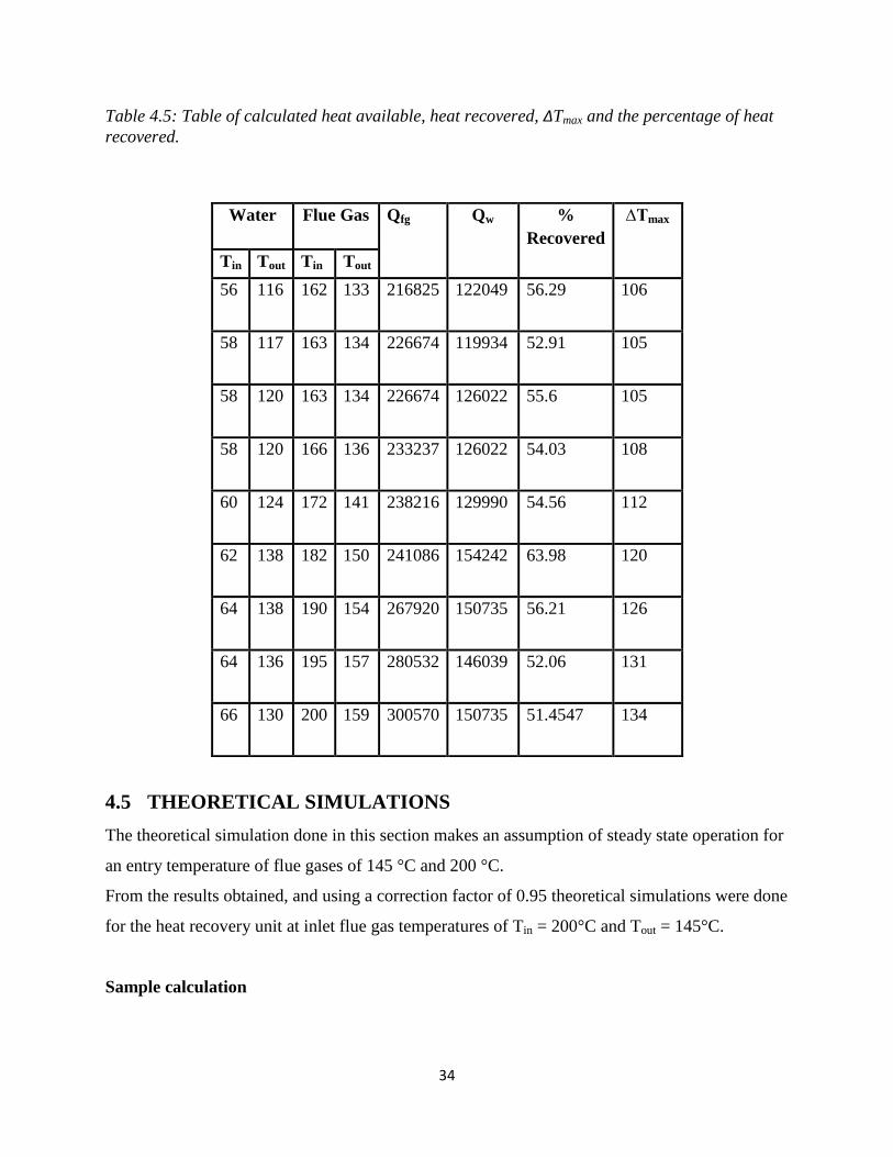
Table 4.5: Table of calculated heat available, heat recovered, ∆Tmax and the percentage of heat
recovered. ...................................................................................................................................... 34
Table 4.6: Table of calculated heat available, heat recovered, percentage of heat recovered and
corresponding Ps values for Tfgin = 200°C .................................................................................... 35
1
CHAPTER ONE: INTRODUCTION
Industrial waste heat refers to energy that is generated in industrial processes without being put
into practical use. Sources of waste heat include hot combustion gases discharged to the
atmosphere, products exiting industrial processes and heat transfer from hot equipment surfaces.
According to a report done by the United States Department of energy,1 it is estimated that
between 20 to 50% of industrial energy input is lost as waste heat in the form of hot exhaust
gases, cooling water and heat lost from hot equipment surfaces through conduction convection
and radiation, heated product streams and products.In order to improve energy efficiency, focus
has been laid on reducing energy consumed by equipment or changing processes or techniques to
manufacture products to make them more energy efficient.
To improve the overall efficiency, waste heat can be captured and reused. The recovered
wasteheat is then used for air/ feed water preheating, water heating or power generation. This in
effect leads to increase in efficiency for processes, greenhouse gas free source of energy and
reduction of energy costs for industries.
This project involves a commercial rotary kiln incinerator that is currently being commissioned.
It is owned by Environmental and Combustion Consultants Limited. The incinerator burns
various industrial and chemical wastes at high temperatures. The flue gases released are at a high
temperature and they form a viable source of waste heat. Aheat recovery unit has been installed
along the chimney line, which in design is a double helical coil heat exchanger. Water passing in
the heat exchanger is heated by the hot flue gases. It is from the total heat gained by the water
that the total energy recovered can be determined. From the data obtained and theoretical
analysis done, a proposal for an end use for the water or steam coming out of the heat recovery
unit will be done.
1 BCS, Incorporated (2008) Waste Heat Recovery: Technology and Opportunities in U.S. Industry, U.S. Department
of Energy
2
1.1 STATEMENT OF THE PROBLEM
The commercial incinerator burns various industrial wastes at high temperatures of up to 1200°C
converting various industrial and chemical wastes to ash and flue gases. The flue gases being
released from combustion are at high temperatures.
In many industries, power cost is a key component of the total production and operations costs.
Currently the cost per kWh is KES 82 for a C12 (Commercial 11kV establishment)which is the
classification of the establishment in terms of power ratings. On average 50,000 kWh are used
monthly. This leads to electricity bills incurred to excess of KES 400,000. With the presence of
a hot flue gas stream that is released to the atmosphere from the combustion of the wastes,
viability of the hot flue gases being used to heat water to steam which can be investigated for
potential use in electricity generation.
One disadvantage of releasing the flue gases to the environment at such high temperatures is that
they may have a negative impact on the environment in terms of air pollution. According to
Justin Hill (2011), the impact of energy dissipated as heat into the atmosphere has also been
explored as a possible source of manmade climate change. This released energy has long been
considered as a main cause to the “heat island” in highly industrialized cities.Releasing flue
gases at a lower temperature to the atmosphere leads to a reduction of the “heat island” effect on
the surface of the earth. This has a contribution in reducing global warming.
In an effort to reduce the exit gas temperatures from the chimney and as a long term effort to
reduce energy costs while providing an alternate source of income, the heat recovery unit aids in
cooling the flue gases while at the same time utilizing the hot flue gas stream to heat water
tosteam. From the inlet and exit temperatures of the water passing through the heat recovery unit,
it is possible to determine the total amount of heat recovered. This is the data that will be used in
coming up with theoretical simulations of the heat recovery unit.
2Electricity costs in Kenya accessed from urlhttps://stima.regulusweb.com/ on 6
th April 2015

3
1.2 OBJECTIVES
The objective of this project is to determine the amount energy recoverable from a flue gas
stream. Our aim will be to carry out:
Carry out a feed water analysis of the borehole water on site and propose a water
treatment method.
Experimental determination of the temperature of the water at the inlet and outlet of the
heat recovery unit at different flue gas inlet and exit temperatures.
Theoretical calculation of the correction factor (F)of the helical heat exchanger, energy
available from the flue gas stream and the energy recovered by the water.
Determination of the heat exchanger effectiveness (ε) at different flue gas temperatures.
Determination of the most optimum heat that can be recovered from theoretical
simulation.
1.3 METHODOLOGY
Literature review from various text books, designs (for example the steam plant in the
thermodynamics lab), standards and articles.
Experimental determination of the temperature of the water at the outlet of the heat
recovery unit.
Theoretical simulations using Microsoft Excel for the most optimum heat that can be
recovered.
1.4 FIELD STUDY
The field study involved taking temperature readings from thermocouples of the flue gas
stream and water.
A survey of a similar plant was also done in East Africa Portland Cement where a similar
project will be undertaken.
The only form of data acquisition was through reading of values from thermocouples,
pressure gauges and water flow meter.
4
1.5 PROJECT JUSTIFICATION
From the experimental data obtained and from the corresponding theoretical analysis, the project
will seek to find out the most optimum energy that can be recovered. If the energy recoverable is
viable for power generation, a proposal can be made to design a steam power plant on site. This
will cut down on the cost of power that the company pays to run machinery on site. Surplus
power can be sold to the national power supplier, Kenya Power providing an alternative source
of income.
For example, a heat recovery boiler/steam turbine WHP project at a petroleum coke plant in Port
Arthur, Texas, recovers energy from 2,000oF exhaust from three petroleum coke calcining
kilns.The project produces 450,000 lb/hr of steam for process use at an adjacent refinery and 5
MW of power.
1.6 PROJECT LIMITATIONS
The flow rate of the water could not be varied independently thereby making it difficult to obtain
data at different water flow rates.
The actual flue gas flow rate could not be measured. The induced draft fan was run at 80% flow
rate capacity at all times while performing the experiment.
The construction of the plant was finished in early March and was commissioned around the
same time. During commissioning, various problems arose, mainly due to the thermocouples
being faulty and sometimes completely failing. This hindered us from obtaining more results
from the site.

5
CHAPTER TWO: LITERATURE REVIEW
Heatrecovery from waste gas sources provides an opportunity for economical operation and
increased efficiency of thermal systems. Energy present in waste gases cannot be fully
recovered. To determine whether a Heatrecovery project is viable, a few important parameters
must be determined3.
2.1 FACTORS AFFECTING WASTE HEAT RECOVERY FEASIBILITY
a) Heat quantity
This is the amount of energy in a waste heat stream. It is given by:
𝑄 = 𝑚 𝐶𝑝∆𝑇 𝐸𝑞𝑢𝑎𝑡𝑖𝑜𝑛 1(𝑎)
Or
𝑄 = 𝑚∆ 𝑡 𝐸𝑞𝑢𝑎𝑡𝑖𝑜𝑛 1 (𝑏)
Where:
Q- Quantity of waste heat in waste heat stream (J/s)
m- Mass flow rate of waste heat stream (Kg/s)
Cp- Specific heat capacity at constant pressure (Joules/Kg.K)
∆T- Change in temperature of waste heat stream (∆K)
∆h- Change in enthalpy as a function of temperature of waste heat stream
b) Heat quality/ temperature
It is the usefulness of the waste heat stream. The temperature difference between the heat source
and sink determines the waste heat’s utility or quality, heat transfer rate per unit surface area (the
smaller the temperature difference the larger the heat exchange surface area required), maximum
theoretical efficiency material selection in heat exchanger design.
Generally waste heat recovery opportunities are categorized into high (649°C and higher),
medium (232°C to 649°C) and low (232°C) and lower.
3Reiter S: 1983
6
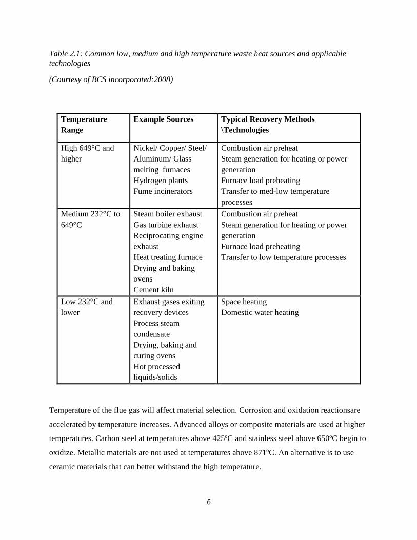
Table 2.1: Common low, medium and high temperature waste heat sources and applicable
technologies
(Courtesy of BCS incorporated:2008)
Temperature
Range
Example Sources Typical Recovery Methods
\Technologies
High 649°C and
higher
Nickel/ Copper/ Steel/
Aluminum/ Glass
melting furnaces
Hydrogen plants
Fume incinerators
Combustion air preheat
Steam generation for heating or power
generation
Furnace load preheating
Transfer to med-low temperature
processes
Medium 232°C to
649°C
Steam boiler exhaust
Gas turbine exhaust
Reciprocating engine
exhaust
Heat treating furnace
Drying and baking
ovens
Cement kiln
Combustion air preheat
Steam generation for heating or power
generation
Furnace load preheating
Transfer to low temperature processes
Low 232°C and
lower
Exhaust gases exiting
recovery devices
Process steam
condensate
Drying, baking and
curing ovens
Hot processed
liquids/solids
Space heating
Domestic water heating
Temperature of the flue gas will affect material selection. Corrosion and oxidation reactionsare
accelerated by temperature increases. Advanced alloys or composite materials are used at higher
temperatures. Carbon steel at temperatures above 425ºC and stainless steel above 650ºC begin to
oxidize. Metallic materials are not used at temperatures above 871ºC. An alternative is to use
ceramic materials that can better withstand the high temperature.

7
c) Waste Stream Composition
The composition of the stream affects the recovery process, material selection, thermal
conductivity and heat capacity. Heat transfer rates in heat exchangers are dependent on the
composition and phase of waste heat streamsand deposition of any fouling substances. Denser
fluids have higher heat transfer coefficients, which enables higher heat transfer rates per unit area
for a given temperature difference.
d) Minimum allowed temperature
This is determined by the flue gas composition. Flue gases contain varying concentrations of
carbon dioxide, water vapor, NOX, SOX, un-oxidized organics and minerals. If the flue gases are
cooled below the dew point temperature, the water vapor in the gas will condense and deposit
corrosive substances on the heat exchanger surface. Heat exchangers are generally designed to
maintain exhaust temperatures above the condensation point.
e) Other factors
Operating schedules: If a waste heat source is only available for a limited time every day, the
heat exchanger may be exposed to both high and low temperatures. One must ensure that the
heat exchange material does not fatigue doe to thermal cycling.
Accessibility: Physical constraints created by equipment arrangements prevent easy access to the
heat source, or prevent the installation of any additional equipment for recovering the heat.
2.2 BENEFITS OF WASTE HEAT RECOVERY
a) Reduced fuel consumption that leads to reduced CO2 emissions.
b) Reduction in equipment sizes of all flue gas handling equipment such as fans, stacks, ducts,
burners etc. due to reduced flue gas produced.
c) It leads to an increase in efficiency. For example, in industrial furnaces, when heat recovery
is done, it leads to an improvement of energy efficiency by 10% to 50%. It also leads to a
reduction in auxiliary energy consumption.
d) It leads can lead to substantial fuel savings. Fuel consumption of a boiler can be reduced by
using waste heat from the plant for preheating both air and boiler feed water.
e) Plants generate their own electricity by using the energy recovered in the form of superheated
steam which runs a turbine.

8
2.3 BARRIERS TO WASTE HEAT RECOVERY
a) Long payback periods due to the high operating, maintenance and materials costs that are
incurred during operation.
b) No direct use in industries for low temperature range flue gas streams.
c) Presence of flue gases with a high chemical activity that will lead to high rates of fouling and
corrosion of the heat recovery unit.
d) It is difficult to access and recover heat from unconventional sources such as hot solid
product streams and hot equipment surfaces and limited space to install waste heat recovery
devices.
A major disadvantage of heat recovery processes is that they reduce the rate of dispersion of
various toxic gases (for example NOX). The heat recovery process in itself does not reduce air
pollution.
A study was conducted on the effect of Heat recovery from flue gases on local humidity and NOx
dispersion in a power plant in Korea4. It was seen that at 115 °C the flue gas containing nitrogen
oxides would be instantaneously diluted at least 60 times as soon as released from the stack. The
direct influencing area was found to be a distance up to 700 m from the emission stack. It
however, stretched over 900m when the flue gas was cooled to 40°C. The lowering of flue gas
temperature therefore, caused an increase in NOx concentration in the region near the power
plant.
4Shi Chang WU, Young Min Jo (2013) Effect of Heat Recovery from flue gas on local humidity and NOx dispersal
in a thermal power station doi: 10.4209/aaqr.2013.01.0028

9
2.4 HEAT EXCHANGER ANALYSIS
Most heat recovery technologies make use of heat exchangers. They facilitate effective heat
transfer between two fluids. Heat transfer is mainly through convection and conduction.
2.4.1 CLASSIFICATION OF HEAT EXCHANGERS
Heat exchangers may be classified according to5:
Nature of heat exchange process
Direct contact heat exchangers- Energy transfer between the hot and cold fluid is brought
about by their complete physical mixing.
Regenerator- A hot fluid is passed through a matrix. Heat is transferred to the solid matrix and
accumulates there. A cold fluid is then passed over the heated matrix and heat is transferred to it
by the matrix.
Recuperator- Fluids flow simultaneously on either side of a separating wall. Heat transfer
occurs between the fluid streams without mixing or physical contact with each other.
Flow arrangement
In the parallel flow heat exchanger, both hot and cold fluids enter the heat exchanger at the
same end and move in the same direction while in the counter flow, the hot and cold fluids enter
the heat exchanger at opposite ends and flow in opposite directions6
Fig2.1: Parallel (a) and counter-flow (b) heat exchanger
(Courtesy of Heat Transfer by Cengel Y.A 2002)
5R.K. Rajput 6Cengel Y.A. 2002

10
Construction
Double Pipe heat exchangers- It is made of two concentric pipes of different diameters where
one fluid flows through the annulus space between the two pipes and the other in the smaller
pipe.
Shell and Tube heat exchangers- They contain a large number of tubes packed in a shell with
their axes parallel to that of the shell. Baffles are placed in the shell to force the shell side fluid to
flow across the shell to enhance heat transfer and to maintain uniform spacing between the tubes.
They are further classified according to the number of shell and tube passes involved.
Plate heat exchangers- They are constructed of thin plates which may be smooth or corrugates.
Hot and cold fluids flow in alternate passages thus each cold fluid stream is surrounded by two
hot fluid steams, resulting in very effective heat transfer.
Heat transfer mechanism
Single phase heat exchanger has no change in phase in both fluids in the heat exchanger while
in the phase change heat exchanger; there is a change in phase in either of the fluids flowing in
the heat exchanger for example, evaporators and condensers.
Compactness
Compact heat exchanger- It has a large heat transfer surface area per unit volume and they are
commonly used in applications with strict limitations on the weight and volume of the heat
exchanger. The ratio of the heat transfer surface area of a heat exchanger to its volume is called
the area density β. Heat exchangers with β > 700m2/m
3 is classified as a compact heat exchanger
e.g. car radiator. Flow in compact heat exchangers may be classified as:
Mixed cross flow- The fluid is free to move in the transverse direction
Unmixed cross flow- Plate fins force the fluid to flow through a particular inter-fin spacing and
prevent it from moving in the transverse direction.

11
In the analysis of a heat exchanger using the log mean temperature difference and ε-NTU
method, the following assumptions are made7
1. The heat exchanger operates under quasi-steady-state conditions (i.e. Constant mass flow
rates)
2. The outside walls are adiabatic. Thereby heat loss or heat gain to the surrounding is
negligible and no thermal energy sources within the heat exchanger.
3. Wall thermal resistance is distributed uniformly in the entire exchanger.
4. Longitudinal heat conduction in the fluids and in the wall is negligible.
5. No phase change occurs in the regenerator.
6. Heat transfer coefficients between the fluids and the matrix wall are constant throughout the
exchanger.
2.4.2 OVERALL HEAT TRANSFER COEFFICIENT
The overall heat transferred between two fluids is given by:
𝑄 = 𝑈𝐴𝜃𝐶𝑂𝑅 = 𝜃𝐶𝑂𝑅𝑅𝑇𝑂𝑇
𝐸𝑞𝑢𝑎𝑡𝑖𝑜𝑛 2
Where:
RTOT- Total thermal resistance
U- Overall heat transfer coefficient
A- Exchange surface area between two fluids.
θCOR- Corrected log mean temperature difference
From equation 4, the relation RTOTand UA is:
𝑅𝑇𝑂𝑇 = 1
𝑈𝐴 𝐸𝑞𝑢𝑎𝑡𝑖𝑜𝑛 3
Heat is transferred from a fluid to the wall by convection, through the wall by conduction and
from the wall to another fluid again by convection. Any radiation effects are usually included in
the convection heat transfer coefficients.
Layers of deposits on the heat transfer surfaces cause the rate of heat transfer in a heat exchanger
to decrease resulting to fouling. This introduces a fouling factor Rf (on the inner and outer
surfaces) which is a measure of the thermal resistance introduced by fouling. It is caused by
scaling, particulate fouling, corrosion and solidification fouling.
The total thermal resistance may be given by:
7Shar R., Dusan P. S 2003; Cengel Y.A. 2002

12
RTOT = Convective Resistance (inside) + Fouling resistance (inside) + Thermal resistance (material) +
Fouling resistance (outside) + Convective thermal resistance (outside)
For a tube, the transfer area is not uniform and U may be defined in terms of the internal Ui or
external Uo areas of the pipe.
Therefore we have:
𝑅𝑇𝑂𝑇 = 1
2𝜋𝑟𝑖𝐿𝑖+
𝑅𝑓𝑖
2𝜋𝑟𝑖𝐿+
1
2𝜋𝐿𝑘𝑙𝑛𝑟𝑜𝑟𝑖
+ 𝑅𝑓𝑜
2𝜋𝑟𝑜𝐿+
1
2𝜋𝑟𝑜𝐿𝑜=
1
𝐴𝑖𝑈𝑖=
1
𝐴𝑜𝑈𝑜 𝐸𝑞𝑢𝑎𝑡𝑖𝑜𝑛 4
Where
hi and ho -Convection heat transfer coefficients for the inside and outside surfaces of the heat
exchanger tubes.
Rfi and Rfo- Fouling resistances due to deposits and other modifications on the surface
k- Thermal conductivity
Dividing the above equation by the internal and external areas where Ai = 2πriL and Ao = 2πroL
we obtain the expression for Uias8
𝑈𝑖 = 1
1
𝑖+ 𝑅𝑓𝑖 +
𝑟𝑖
𝑘ln
𝑟𝑜
𝑟𝑖+
𝑟𝑖
𝑟𝑜𝑅𝑓𝑜 +
𝑟𝑖
𝑟𝑜𝑜
𝐸𝑞𝑢𝑎𝑡𝑖𝑜𝑛 5
The expression for Uo is then obtained as:
𝑈𝑜 = 1
𝑟𝑜
𝑟𝑖𝑖+
𝑟𝑜
𝑟𝑖𝑅𝑓𝑖 +
𝑟𝑜
𝑘ln
𝑟𝑜
𝑟𝑖+ 𝑅𝑓𝑜 +
1
𝑜
𝐸𝑞𝑢𝑎𝑡𝑖𝑜𝑛 6
2.4.3 USE OF THE LOG MEAN TEMPERATURE DIFFERENCE (LMTD) AND
ε-NTU METHOD IN HEAT EXCHANGER ANALYSIS
2.4.3.1 LOG MEAN TEMPERATURE DIFFERENCE (LMTD)
Consider a double pipe counter flow heat exchanger as shown below. The hot fluid passes
through the smaller pipe and the cold fluid passes through the annulus of the larger pipe.
8Luti F.M 2012

13
Fig 2.2: Double pipe counter flow heat exchanger
(Courtesy of Heat Transfer by Cengel Y.A 2002)
From the log mean temperature difference (LMTD) method of analysis, the total heat transferred
may be given by:
𝑄 = 𝑈𝐴𝜃𝑀 𝐸𝑞𝑢𝑎𝑡𝑖𝑜𝑛 7
Where θM is the log mean temperature difference. This is given by:
𝜃𝑀 = ∆𝑇1 − ∆𝑇2
𝑙𝑛 ∆𝑇1
∆𝑇2
𝐸𝑞𝑢𝑎𝑡𝑖𝑜𝑛 8
∆T1 and ∆T2 are the temperature differences at the inlet and outlets of the heat exchangers.
The above expression is limited to parallel flow and counter flow heat exchangers only.
However, various expressions have been made for cross flow and multi-pass shell and tube heat
exchangers. The resulting expressions are too complicated because of complex flow conditions.
It is therefore convenient to relate equivalent temperature difference to LMTD relation for
counter flow case as:
𝜃𝐶𝑂𝑅𝑅 = 𝐹𝜃𝑀 𝐸𝑞𝑢𝑎𝑡𝑖𝑜𝑛 9
Where F is the correction factor
This is a measure of deviation of the θM for corresponding values of the counter flow case. F is a
function of the geometry plus two parameters P and R. Therefore,
𝐹 = 𝑓(𝑅,𝑃,𝑔𝑒𝑜𝑚𝑒𝑡𝑟𝑦) 𝐸𝑞𝑢𝑎𝑡𝑖𝑜𝑛 10
Where:
𝑅 = (𝑇𝑖𝑛 − 𝑇𝑜𝑢𝑡 )𝑠𝑒𝑙𝑙(𝑇𝑜𝑢𝑡 − 𝑇𝑖𝑛 )𝑡𝑢𝑏𝑒
= (𝑚 𝐶𝑝)𝑡𝑢𝑏𝑒
(𝑚 𝐶𝑝)𝑠𝑒𝑙𝑙 𝐸𝑞𝑢𝑎𝑡𝑖𝑜𝑛 11 (𝑎)
And:

14
𝑃 = (𝑇𝑜𝑢𝑡 − 𝑇𝑖𝑛 )𝑠𝑒𝑙𝑙
(𝑇𝑖𝑛 𝑠𝑒𝑙𝑙 − 𝑇𝑖𝑛 𝑡𝑢𝑏𝑒 ) 𝐸𝑞𝑢𝑎𝑡𝑖𝑜𝑛 11 (𝑏)
2.4.3.2 ε-NTU METHOD
Effectiveness (ε) for a heat exchanger is the ration of the actual heat transfer rate to themaximum
heat transfer possible9.
𝜀 = 𝐴𝑐𝑡𝑢𝑎𝑙 𝑡𝑟𝑎𝑛𝑠𝑓𝑒𝑟 𝑟𝑎𝑡𝑒
𝑀𝑎𝑥𝑖𝑚𝑢𝑚 𝑒𝑎𝑡 𝑡𝑟𝑎𝑛𝑠𝑓𝑒𝑟 𝑟𝑎𝑡𝑒 𝑝𝑜𝑠𝑠𝑖𝑏𝑙𝑒=
𝑄
𝑄𝑀𝐴𝑋 𝐸𝑞𝑢𝑎𝑡𝑖𝑜𝑛 12
QMAX is given by:
𝑄𝑀𝐴𝑋 = 𝐶𝑚𝑖𝑛 𝑇𝑜𝑡 𝑖𝑛 − 𝑇𝑐𝑜𝑙𝑑 𝑖𝑛 = 𝐶𝑚𝑖𝑛 ∆𝑇𝑚𝑎𝑥 𝐸𝑞𝑢𝑎𝑡𝑖𝑜𝑛 13
Where; 𝐶𝑚𝑖𝑛 = 𝑚 ∗ 𝐶𝑝(min )
Equation 12 may be written as:
𝜀 = 𝐶(𝑇𝑖 − 𝑇𝑜)
𝐶𝑚𝑖𝑛 (𝑇𝑖 − 𝑇𝑐𝑖)=
𝐶𝑐(𝑇𝑐𝑜 − 𝑇𝑐𝑖)
𝐶𝑚𝑖𝑛 (𝑇𝑖 − 𝑇𝑐𝑖)=
𝑈𝐴𝐹𝜃𝑀𝐶𝑚𝑖𝑛 ∆𝑇𝑚𝑎𝑥
𝐸𝑞𝑢𝑎𝑡𝑖𝑜𝑛 14
Effectiveness of a heat exchanger enables us to determine the heat transfer rate without knowing
the outlet temperature of the fluids. The effectiveness of a heat exchanger depends on the
geometry of the heat exchanger as well as the flow arrangement.
Effectiveness relations of the heat exchangers typically involve the dimensionless group
UAs/Cmin. This quantity is called the number of transfer units (NTU). Normally for a higher
value of NTU the larger the heat exchanger.
Effectiveness of a heat exchanger is a function of the number of transfer units (NTU), flow
arrangement and the capacity ratio c where c = Cmin/Cmax.
𝜀 = 𝑓 𝑈𝐴𝑠𝐶𝑚𝑖𝑛
, 𝑐 ,𝐹𝑙𝑜𝑤 𝑎𝑟𝑟𝑎𝑛𝑔𝑒𝑚𝑒𝑛𝑡 𝐸𝑞𝑢𝑎𝑡𝑖𝑜𝑛 15
Effectiveness relations have been developed for a large number of heat exchangers.
9Luti F.M 2012

15
2.5 WASTE HEAT RECOVERY TECHNOLOGIES
As earlier stated, most heat recovery technologies make use of heat exchangers. The following
are the common types waste heat recovery technologies10
.
2.5.1 GAS- AIR HEAT RECOVERY TECHNOLOGIES
There are used most commonly used to heat combustion air by heat exchange with flue gas. It is
also used in direct fired air or gas heaters in process work. Some of the technologies used
include:
a) Recuperators
They recover exhaust gas waste heat in medium to high temperatures that is used to preheat air
for combustion. They are constructed of either metallic or ceramic materials. They can generally
be categorized into three:
Metallic radiation recuperator- It consists of two concentric lengths of ductwork. Hot waste gases
pass through the inner duct and heat is radiated to the wall and the cold incoming air in the outer
shell.
Convective or tube type recuperator- Hot gases are carried through a number of parallel small
diameter tubes, while the incoming air to be heated enters a shell surrounding the tubes.
Combined radiation/convection recuperator- The system has a radiation section followed by
convection section.
b) Regenerators
These are heat exchangers through which hot and cold air flow alternatively. Flue gases flow
through one chamber, from where the surfaces absorb heat and increase in temperature. The flow
of air is them adjusted so that so that incoming combustion air passes over the surfaces which
transfers heat to the combustion air entering the furnace.
c) Heat wheel (Rotary Regenerative Heat Exchanger)They make use of a rotating porous
disc of a high heat capacity material placed across two parallel ducts, one containing hot
waste gas the other containing cold gas. The disc rotates between two ducts and transfers heat
from the hot gas duct to the cold gas duct.
10Boyen J.L, 1975; Reiter S. 1983; BCS, Incorporated 2008

16
d) Passive Air Pre-heaters
They are generally of two types:
Plate type exchanger
Heat pipe heat exchanger- It consists of several pipes with sealed ends. Each pipe contains a
capillary wick structure that facilitates movement of the working fluid between the hot and cold
ends of the pipe. Hot gases pass over one end of the heat pipe, causing the working fluid inside
the pipe to evaporate. Pressure gradients along the pipe cause the hot vapor to move to the other
end of the pipe, where the vapor condenses and transfers heat to the cold gas. The condensate
then cycles back to the hot side of the pipe via capillary action.
2.5.2 GAS- WATER HEAT RECOVERY TECHNOLOGIES
a) Boiler feed water preheating (Economizers)
They are found in process boilers where waste heat in the exhaust gas is passed along finned
tubes that carry the boiler feed water. The feed water receives heat from hot gases flowing across
the tubes. The feed water is then fed into the boiler. This in effect increases the efficiency of the
power plant.
2.5.3 POWER GENERATION
This involves using waste heat to heat water forming steam which is expanded in a turbine
coupled to an electric generator. The tubes carry the feed water which is heated and converted to
steam. In cases where the waste heat is not sufficient for producing desired levels of steam,
auxiliary burners or an afterburner can be added to attain a higher steam output.
Generating electrical power via mechanical work makes use of the Steam Rankine Cycle,
Organic Rankine Cycle and the Kalina Cycle.
a) Steam Rankine Cycle
Water/steamis used as the working fluid in the closed loop. Steam is the most common working
fluid used in vapor power cycles because of its many desirable characteristics such as low cost,
availability and high enthalpy of vaporization.
Wateris first pumped to elevated pressure before entering a heat recovery boiler. The pressurized
water is vaporized by the hot exhaust and then expanded to lower temperature and pressure in a
turbine, generating mechanical power that can drive an electric generator. The low-pressure
steam is then exhausted to a condenser at vacuum conditions, where heat is removed by

17
condensing the vapor back into a liquid. The condensate from the condenser is then returned to
the pump and the cycle continues.
This is illustrated in the figure below:
Fig 2.3: The simple ideal Rankine cycle
(Courtesy of Thermodynamics by Cengel Y.A 2002)
Energy analysis of the Ideal Rankine Cycle
The kinetic energy changes are usually small relative to the work and heat transfer terms and are
therefore usually neglected. The steady flow energy equation per unit mass of steam reduced to.
𝑄𝑖𝑛 − 𝑄𝑜𝑢𝑡 + 𝑊𝑖𝑛 −𝑊𝑜𝑢𝑡 = 𝑒 − 𝑖 (𝑘𝐽 𝑘𝑔) 𝐸𝑞𝑢𝑎𝑡𝑖𝑜𝑛 16
Boiler and condenser don’t involve any work, and the pump and the turbine are assumed to be
isentropic. Then the conservation of energy relation for each device can be expressed as follows.
Table 2.2: Energy relation for the devices in a Rankine Cycle
Device Energy Relation
Pump h2-h1 or v(P2-P1) h1 where h1 = hf at P1 and v = vfat P1
Boiler Qin = h3-h2
Turbine Wturbine out = h3-h4
Condenser Qout = h4-h1
18
The thermal efficiency of the Rankine cycle is determined from
𝜂 𝑡 = 𝑊𝑛𝑒𝑡
𝑄𝑖𝑛= 1 −
𝑊𝑖𝑛
𝑄𝑜𝑢𝑡
b) Organic Rankine cycle
Organic working fluids (e.g. ammonia, toluene, Freon, haloalkanes, and iso-pentane)can be used
below a temperature of 400°C.The fluids have better efficiencies at lower heat source
temperatures and have lower boiling point, higher vapor pressure, higher molecular mass, do not
have to be superheated, and higher mass flow compared to water If the degree of superheating is
reduced, more steam can be generated and hence more energy can be recovered from the heat
source. In this cycle, the working fluid superheats as the pressure is reduced unlike steam which
becomes wet during expansion11
.
c) Kalina cycle
The working fluid is an ammonia water mixture. Its main advantage over the conventional
Rankine cycle is that the ammonia water mixture has a varying boiling and condensing
temperature, which enables the fluid to extract more energy from the hot stream by matching the
hot source better than a system with a constant boiling and condensing temperature. This results
in significant energy recovery from hot gas streams, particularly those at low temperatures. It is
15-25% more efficient than the Organic Rankine Cycles working at the same temperature level.
11V. Ganapathy 2003
19
CHAPTER THREE: FEED WATER ANALYSIS
Water treatment and conditioning is the process of making water from any natural source such as
river, dam or lake suitable for feeding water into a boiler and mixing appropriate chemicals to
treated water to prevent damage to internal surfaces of a boiler.
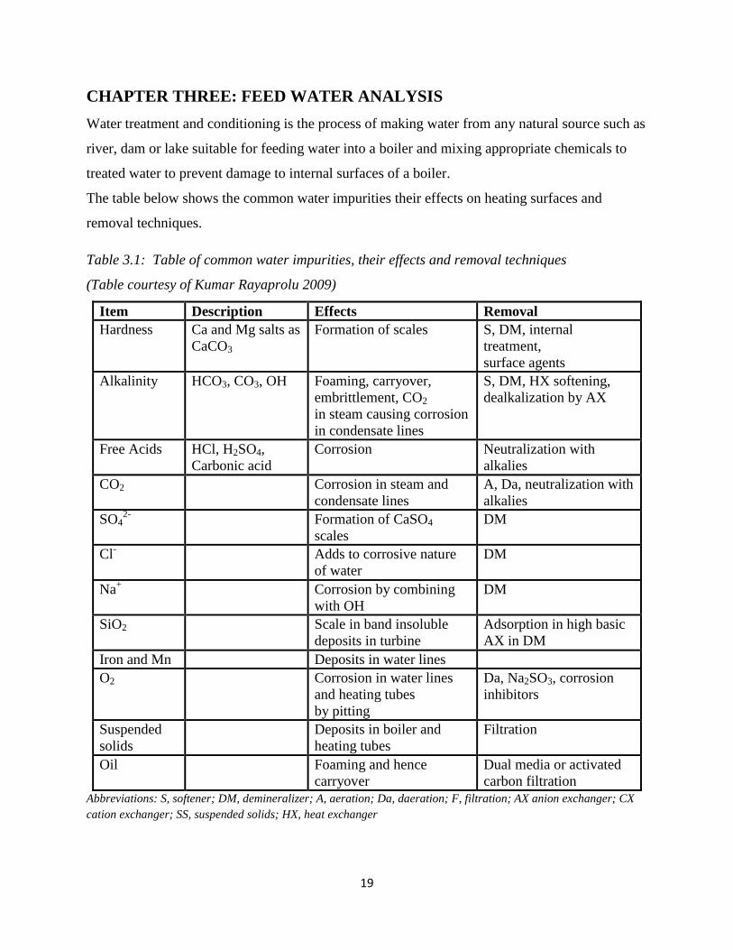
The table below shows the common water impurities their effects on heating surfaces and
removal techniques.
Table 3.1: Table of common water impurities, their effects and removal techniques
(Table courtesy of Kumar Rayaprolu 2009)
Item Description Effects Removal
Hardness Ca and Mg salts as
CaCO3
Formation of scales S, DM, internal
treatment,
surface agents
Alkalinity HCO3, CO3, OH Foaming, carryover,
embrittlement, CO2
in steam causing corrosion
in condensate lines
S, DM, HX softening,
dealkalization by AX
Free Acids HCl, H2SO4,
Carbonic acid
Corrosion Neutralization with
alkalies
CO2 Corrosion in steam and
condensate lines
A, Da, neutralization with
alkalies
SO42-
Formation of CaSO4
scales
DM
Cl-
Adds to corrosive nature
of water
DM
Na+
Corrosion by combining
with OH
DM
SiO2 Scale in band insoluble
deposits in turbine
Adsorption in high basic
AX in DM
Iron and Mn Deposits in water lines
O2 Corrosion in water lines
and heating tubes
by pitting
Da, Na2SO3, corrosion
inhibitors
Suspended
solids
Deposits in boiler and
heating tubes
Filtration
Oil Foaming and hence
carryover
Dual media or activated
carbon filtration
Abbreviations: S, softener; DM, demineralizer; A, aeration; Da, daeration; F, filtration; AX anion exchanger; CX
cation exchanger; SS, suspended solids; HX, heat exchanger
20
3.1 WATER TREATMENT
Water treatment is grouped into two main areas external and internal treatment12
.
3.1.1 EXTERNAL TREATMENT
Its the removal of suspended solids (through sedimentation and filtration) hardness, other soluble
impurities and degasification (Deaeration).
Oxygen scavengers are also used to further remove dissolved oxygen. They can be divided into
non-volatile (e.g. Sodium Sulfite, Iso ascorbic acid and Tannins) and volatile chemicals
(Hydrazine, Diethyl Hydroxylamine (DEHA) and Carbohydrazide).
3.1.1.1 Removal of Hardness
Thiscan be done using the following methods:
a) Lime Softening- Slaked lime (Calcium hydroxide) is added to hard water and it reacts with
some of the calcium, magnesium and silica forming a solid precipitate. The reaction that
takes place as shown below:
Ca OH 2 s + Ca(HCO3)2(aq ) → 2CaCO3(s) + 2H2O(l)
b) Base Exchange Softening- Hard water enters an ion exchange unit that is partially filled
with an ion exchange resin. The calcium and magnesium ions are exchanged for sodium ions.
The resin is regenerated by passing a concentrated solution of sodium chloride (brine)
through it.
c) Dealkalization-Water is passed through a weak acid cation exchanger where calcium and
magnesium ions are exchanged for hydrogen ions. The hydrogen carbonates are converted to
carbonic acid which is removed in a de-gassing tower.
d) Ion exchange demineralization- Water is passed through a one or more cation exchange
beds (calcium and magnesium are exchanged for hydrogen ions) then through anion
exchange beds (sulphate, chloride, carbonate and silica are ex-changed for hydroxide ions).
e) Reverse osmosis- The process makes use of a applying a pressure greater than the osmotic
pressure to a more concentrated solution that is separated from a less concentrated solution
by a semi-permeable membrane. Water from the more concentrated solution is forced back
through the semi permeable membrane to the more dilute solution on the other side. Water
12CIBO Handbook, 1997; Kumar Rayaprolu 2009; BS 2486-1997

21
containing high levels of hardness should be pre-treated prior to being fed to the reverse
osmosis membranes to prevent them becoming fouled with calcium salts or other foulants.
The process is very effective as it removes 95%-99% 13
of all dissolved salts in the water.
3.1.2 INTERNAL TREATMENT/INTERNAL CONDITIONING
This is the dosing of appropriate chemicals at specific places to the treated feed water to prevent
damage to the internal surfaces of the heating surfaces. They assist with managing corrosion,
scaling, removing traces of dissolved O2 and maintain correct chemical balance in feed water.
The four main types are:
a) Conventional Phosphate treatment. A pH of 10.5-11.2 is maintained with excess OH and
converting the hardness constituents as flocculent precipitate. Orthophosphate residuals are
maintained between 20 and 60 ppm as PO4 and hydrate alkalinity.
b) Coordinated Phosphate treatmentChemicals used are a combination of tri- and disodium
phosphates. pH correction is done by altering the ratio of tri- and disodium phosphates.
c) All-volatile treatmentmethod makes use of ammonia and hydrazine.
3.2 CHEMICAL ANALYSIS OF SITE WATER
Table 3.2: Borehole water analysis results
(Courtesy of Aquachem Chemicals)
Parameters Unit Result Parameters Unit Result
Ph pH Scale 8.56 Total Alkalinity mgCaCO3/l 430
Color mgPt/1 <5 Chloride mg/l 600
Turbidity N.T.U. 4.8 Fluoride mg/l 8.99
Conductivity (25°C) µS/cm 2980 Nitrate mg/l 3.36
Iron mg/l 0.2 Nitrite mg/l <0.01
Manganese mg/l <0.01 Sulphate mg/l 166
Calcium mg/l 8.0 Free Carbon Dioxide mg/l NIL
Magnesium mg/l 9.72 Total Dissolved solids mg/l 1847.6
Sodium mg/l 654.6 Arsenic µg/l -
Potassium mg/l 5.1 Others -
Total Hardness mgCaCO3/l 60
13
Basics of reverse osmosis- Accessed from urlhttp://puretecwater.com/resources/basics-of-reverse-osmosis.pdf on
1st October 2014
22
3.3 PROPOSED FEED WATER TREATMENT
In order to perform the experiment, the main feed water problems that must be handled are those
that will cause scaling in the tubes and corrosion. From table 3.2, it’s seen that the amounts of
calcium and magnesium in the site water and the amount of hardness were extremely high.
From BS 2486-199714
, the heat recovery steam unit can be classified as a non-fired water tube
boiler common in heat recovery applications. It is difficult to generalize on the water chemistry
since they cover a wide range of operating pressures designs and applications. Recommended
water standards for a non-fired water boiler is as shown in Appendix A1.
3.3.1 CHEMICAL TREATMENT AGAINST SCALING
The chemical chosen for use was Sodium tri- phosphate (Na3PO4). It prevents scale formation
by converting impurities into a slug that settles at the bottom of the boiler removed by
blowdown15
.
𝐹𝑒𝑒𝑑 𝑟𝑒𝑞𝑢𝑖𝑟𝑚𝑒𝑛𝑡 𝑁𝑎3𝑃𝑂4 = 𝐹𝑊 𝐶𝑎 ∗ 1.15 + 1.7 ∗ 𝑑𝑒𝑠𝑖𝑟𝑒𝑑 𝑃𝑂4−3 𝑟𝑒𝑠𝑖𝑑𝑢𝑎𝑙/𝐶𝑦𝑐𝑙𝑒𝑠
Hardness concentration = 60mgCaCO3/l
Desired residual = 12 mg/L (chosen arbitrarily by the designer to be between 5-30 mg/L)
𝐹𝑒𝑒𝑑 𝑟𝑒𝑞𝑢𝑖𝑟𝑚𝑒𝑛𝑡 𝑁𝑎3𝑃𝑂4 = 60 ∗ 1.15 + 1.7 ∗ 12
1.0336= 88.74 𝑚𝑔/𝑙
To treat 1000 liters of water we use:
88.74 ∗ 10−3 ∗ 1000 = 88.74 𝑔
The chemical dosing of sodium tri-phosphatewas to be done in the upper feed tank.
3.3.2 CHEMICAL TREATMENT AGAINST CORROSION BY OXYGEN
After removal of hardness, the water was channeled to a second tank where oxygen removal was
to be done using Sodium Sulphite.It is very reactive and reduces oxygen to very low levels to
less than 5ppb if used correctly.
The feed requirement for Na2SO3 mg/L per mg/L of dissolved Oxygen is 7.88 mg/L.
Sulfite residual maintained in the boiler is about 5 to 20 mg/L divided by boiler
cycles.(Association of Water Technologies, Technical Manual)
Have the equation below:
14
BS 2486-1997: Recommendations for treatment of water for steam boilers and water heaters 15
Association of Water Technologies, Technical Manual

23
𝐹𝑒𝑒𝑑 𝑟𝑒𝑞𝑢𝑖𝑟𝑚𝑒𝑛𝑡 (𝑁𝑎2𝑆𝑂3) = 7.88 ∗ 𝑚𝑔 𝐿 𝑂2 + 5 − 20𝑚𝑔 𝐿
𝐵𝑜𝑖𝑙𝑒𝑟 𝐶𝑦𝑐𝑙𝑒𝑠
Taking the feed water to be at a temperature of 20°C, oxygen content is 10 mg/l.
Residual SO3 taken as 6 mg/L (chosen arbitrarily by the designer to be between 5-20 mg/L)
From the water analysis done:
The total dissolved solids 1847.6mg/l
The total hardness 60mg/l
Theoretical Boiler cycles;
𝐵𝑜𝑖𝑙𝑒𝑟 𝐶𝑦𝑐𝑙𝑒𝑠 = 𝐵𝐷 𝐶𝑜𝑛𝑐𝑒𝑛𝑡𝑟𝑎𝑡𝑖𝑜𝑛
𝐹𝑊 𝐶𝑜𝑛𝑐𝑒𝑛𝑡𝑟𝑎𝑡𝑖𝑜𝑛=
1847.6
1787.6= 1.0336
Feeding the values in the feed requirement equation we have:
𝐹𝑒𝑒𝑑 𝑟𝑒𝑞𝑢𝑖𝑟𝑚𝑒𝑛𝑡 (𝑁𝑎2𝑆𝑂3) = 7.88 ∗ 10 + 6
1.0336
𝐹𝑒𝑒𝑑 𝑟𝑒𝑞𝑢𝑖𝑟𝑚𝑒𝑛𝑡 𝑁𝑎2𝑆𝑂3 = 78.8 + 5.7477 = 84.6052 𝑚𝑔/𝑙
To treat 1000 liters of water we use:
84.6052 ∗ 10−3 ∗ 1000 = 84.6052 𝑔
For the experimental setup, the main aim here was to treat the feed water to prevent scaling and
corrosion. From the water analysis results done, it can be seen that the chloride concentration is
very high (600 mg/l). This may have little effect in terms of corrosion and scaling boiler feed
water problems. However, when a turbine is installed, the chloride ions may cause priming when
they settle on the turbine blades leading to a decline in turbine efficiency.
24
CHAPTER FOUR: RESULTS AND ANALYSIS
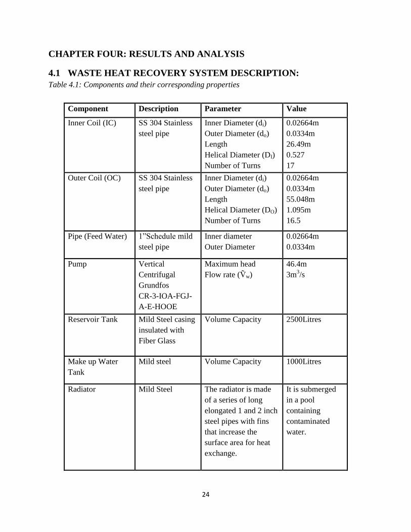
4.1 WASTE HEAT RECOVERY SYSTEM DESCRIPTION:
Table 4.1: Components and their corresponding properties
Component Description Parameter Value
Inner Coil (IC) SS 304 Stainless
steel pipe
Inner Diameter (di)
Outer Diameter (do)
Length
Helical Diameter (DI)
Number of Turns
0.02664m
0.0334m
26.49m
0.527
17
Outer Coil (OC) SS 304 Stainless
steel pipe
Inner Diameter (di)
Outer Diameter (do)
Length
Helical Diameter (DO)
Number of Turns
0.02664m
0.0334m
55.048m
1.095m
16.5
Pipe (Feed Water) 1”Schedule mild
steel pipe
Inner diameter
Outer Diameter
0.02664m
0.0334m
Pump Vertical
Centrifugal
Grundfos
CR-3-IOA-FGJ-
A-E-HOOE
Maximum head
Flow rate (Ṽw)
46.4m
3m3/s
Reservoir Tank Mild Steel casing
insulated with
Fiber Glass
Volume Capacity 2500Litres
Make up Water
Tank
Mild steel Volume Capacity
1000Litres
Radiator Mild Steel The radiator is made
of a series of long
elongated 1 and 2 inch
steel pipes with fins
that increase the
surface area for heat
exchange.
It is submerged
in a pool
containing
contaminated
water.

25
Fig 4:13D representation of the helical coil heat exchanger
4.2 RESULTS
Table 4.2: Results as obtained from site
Water Flue Gas
Tin Tout Tin Tout
56 0C 116
0C 162
0C 133
0C
580C 117
0C 163
0C 134
0C
58 0C 120
0C 163
0C 134
0C
58 0C 120
0C 166
0C 136
0C
60 0C 124
0C 172
0C 141
0C
620C 138
0C 182
0C 150
0C
64 0C 138
0C 190
0C 154
0C
64 0C 136
0C 195
0C 157
0C
660C 130
0C 200
0C 159
0C
Induced draft fan flow rate = Ṽfg = 24,000Cfm
The IDFan was run at 80 % capacity, hence the flow rate was taken as Ṽfg = 0.8*24,000= 19,200
cfm and at a pressure of about 0.99 Bar.
Water flow rate = Ṽw= 1.783m3/hr
26
Pump Pressure (Gauge) = 2 Bar
4.3 DATA ANALYSIS
4.3.1 AREA CALCULATION
Total inner area (Ai):
2.217 + 4.6071 = 6.8241 𝑚2
Total outer area (Ao):
2.7796 + 5.7761 = 8.5557 𝑚2
4.3.2 SINGLE PHASE ANALYSIS FOR THE HEAT RECOVERY UNIT
The analysis below was done for the heat exchanger in single phase. (i.e. The water did not
change phase)
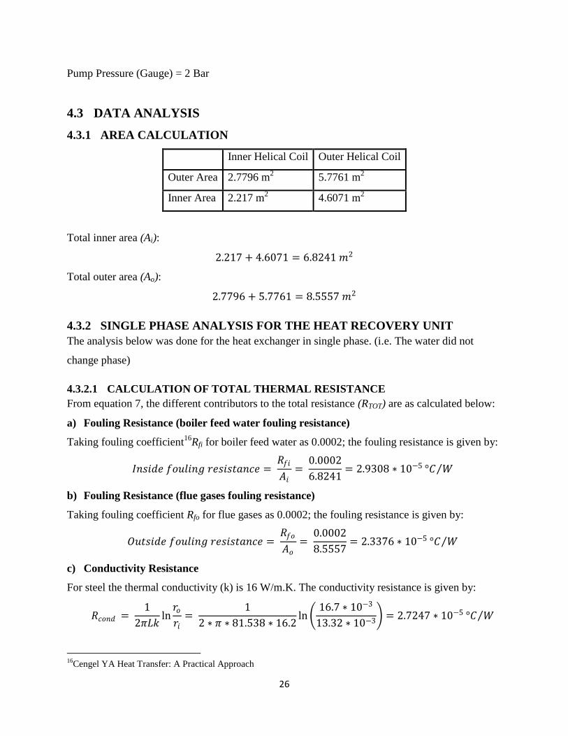
4.3.2.1 CALCULATION OF TOTAL THERMAL RESISTANCE
From equation 7, the different contributors to the total resistance (RTOT) are as calculated below:
a) Fouling Resistance (boiler feed water fouling resistance)
Taking fouling coefficient16
Rfi for boiler feed water as 0.0002; the fouling resistance is given by:
𝐼𝑛𝑠𝑖𝑑𝑒 𝑓𝑜𝑢𝑙𝑖𝑛𝑔 𝑟𝑒𝑠𝑖𝑠𝑡𝑎𝑛𝑐𝑒 = 𝑅𝑓𝑖
𝐴𝑖=
0.0002
6.8241= 2.9308 ∗ 10−5 °𝐶 𝑊
b) Fouling Resistance (flue gases fouling resistance)
Taking fouling coefficient Rfo for flue gases as 0.0002; the fouling resistance is given by:
𝑂𝑢𝑡𝑠𝑖𝑑𝑒 𝑓𝑜𝑢𝑙𝑖𝑛𝑔 𝑟𝑒𝑠𝑖𝑠𝑡𝑎𝑛𝑐𝑒 = 𝑅𝑓𝑜
𝐴𝑜=
0.0002
8.5557= 2.3376 ∗ 10−5 °𝐶 𝑊
c) Conductivity Resistance
For steel the thermal conductivity (k) is 16 W/m.K. The conductivity resistance is given by:
𝑅𝑐𝑜𝑛𝑑 = 1
2𝜋𝐿𝑘ln𝑟𝑜𝑟𝑖
= 1
2 ∗ 𝜋 ∗ 81.538 ∗ 16.2ln
16.7 ∗ 10−3
13.32 ∗ 10−3 = 2.7247 ∗ 10−5 °𝐶 𝑊
16
Cengel YA Heat Transfer: A Practical Approach
Inner Helical Coil Outer Helical Coil
Outer Area 2.7796 m2 5.7761 m
2
Inner Area 2.217 m2 4.6071 m
2

27
d) Convective Heat Transfer Resistance (Inside the helical heat exchanger)
Assumptions made in the flow are that the flow rate remains constant.
Velocity of flow of water:
𝑣𝑤 = 𝑉 𝑤
𝑇𝑢𝑏𝑒 𝑐𝑟𝑜𝑠𝑠𝑒𝑐𝑡𝑖𝑜𝑛 𝑎𝑟𝑒𝑎=
1.78299/3600
𝜋 ∗ 0.013322= 0.88856 𝑚/𝑠
Calculating the convective heat transfer coefficient
The convective heat transfer coefficient is a function of Reynolds number and Prandtl number.
The two terms vary with temperature of the fluid flowing in the tube.
Mori and Nakayama17
(1967b) proposed a formula relating the Nusselt number of flow in a
helical heat exchanger with Reynolds number, Prandtl the ratio (D/d). It is given by:
𝑁𝑢𝑐 = 0.023 1 + 0.061
𝑅𝑒 𝑑 𝐷 2.5 1 6 𝑑 𝐷
1
12𝑅𝑒0.833𝑃𝑟0.4
The above equation is valid for:
𝑃𝑟 > 1, 𝑅𝑒(𝑑 𝐷 ) > 0.4
Sample calculation
Taking the temperatures at Tin = 56°C and Tout = 116°C for water:
Mean bulk temperature of the water flowing inside the helical heat exchanger coil:
𝑇𝑀𝐵 = 56 + 116
2= 86℃
Cp at mean bulk temperature is 4204 J/kgK and density at the mean bulk temperature is 968.244
kg/m3.
In order to use the Nusselt number relation developed by Mori and Nakayama (1967b), the
helical heat exchanger can be analyzed as two separate heat exchangers that are arranged in
series.
i. Inner helical coil analysis
An assumed mean bulk temperature of the inner helical heat exchanger coil is given by:
𝑇𝑀𝐵𝐼 = 56 + 86
2= 71℃
17Mori and Nakayama Coronel P., Sandeep K.P.: Heat transfer coefficient in Helical Heat Exchangers under
Turbulent Flow conditions

28
Properties of the water at 71°C: Density (ρ) = 976.9455 Kg/m3, Specific heat capacity at constant
pressure (Cp) = 4191 J/Kg.K, Dynamic viscosity (µ) = 0.0003948 kg/ms, Prandtl number (Pr) =
2.4968, thermal conductivity (k) = 0.6628.
Reynolds number:
𝑅𝑒𝐼 = 𝜌𝑑𝑣𝑤𝜇
= 976.9455 ∗ 0.02664 ∗ 0.88856
0.0003948= 58575.76
The ratio (di/DI)
𝑑𝑖𝐷𝐼
= 0.02664
0.527= 0.05055
Substituting the above values in the relation developed by Mori and Nakayama:
𝑁𝑢𝑐 = 0.023 1 + 0.061
58575.76 0.05055 2.5 1 6 0.05055
1
12 ∗ 58575.760.833 ∗ 2.49680.4
= 250.4163
Convective heat transfer coefficient can be obtained by the relation below:
𝑁𝑢𝑐 =𝐼𝑑𝑖𝑘
= 250.4163 ∴ 𝑐 = 6230.329 𝑊/𝑚2℃
ii. Outer helical coil analysis
Mean bulk temperature of the outer helical heat exchanger coil:
𝑇𝑀𝐵𝑂 = 86 + 116
2= 101℃
Properties of the water at 101°C: Density (ρ) = 957.1232 Kg/m3, Specific heat capacity at
constant pressure (Cp) = 4220.4 J/Kg.K, Dynamic viscosity (µ) = 0.0002762 kg/ms, Prandtl
number (Pr) = 1.7107, thermal conductivity (k) = 0.6814.
Reynolds number:
𝑅𝑒𝐼 = 𝜌𝑑𝑣𝑤𝜇
= 957.1232 ∗ 0.02664 ∗ 0.88856
0.0002432= 82029.28
The ratio (di/DO)
𝑑𝑖𝐷𝑂
= 0.02664
1.095= 0.024329
Substituting the above values in the relation developed by Mori and Nakayama18
:
18
Mori and Nakayama adapted from Coronel P., Sandeep K.P.: Heat transfer coefficient in Helical Heat Exchangers
under Turbulent Flow conditions

29
𝑁𝑢𝑐 = 0.023 1 + 0.061
82029.28 0.024329 2.5 1 6 0.024329
1
12 82029.280.833 1.71070.4
= 270.6131
Convective heat transfer coefficient can be obtained by the relation below:
𝑁𝑢𝑐 =𝑂𝑑𝑖𝑘
= 270.6131 ∴ 𝑐 = 6921.763 𝑊/𝑚2℃
Adding the inside and outside helical convective heat transfer coefficient inside the tubes we
obtain:
𝑇𝑂𝑇 = 6230.329 + 6921.763 = 13152.09148 𝑊/𝑚2℃
Convective heat resistance (inside the tubes) is given by:
1
𝐴𝑖𝑖=
1
6.8241 ∗ 20224.2567= 1.11419 ∗ 10−5
e) Convective Heat Transfer Resistance (Flow over the helical coil heat exchanger)
Assumptions made in the flow over the helical coil heat exchanger are the flow rate of the flue
gases is constant.
Flue gas velocity:
𝑣𝑓𝑔 = 𝑉 𝑓𝑔
𝑇𝑢𝑏𝑒 𝑐𝑟𝑜𝑠𝑠𝑒𝑐𝑡𝑖𝑜𝑛 𝑎𝑟𝑒𝑎=
19200 ∗ 1.699/3600
𝜋 ∗ 0.62= 8.01198 𝑚/𝑠
Consider the diagram below:
Fig 4:2 Flow over in line series of tube banks
(Courtesy of Heat Transfer by Cengel Y.A 2002)

30
The maximum velocity for an inline flow as in the case above can be approximated at the point
where the separation distance between the inner and outer helical coil is minimum. Have
maximum velocity calculated as:
𝑣𝑚𝑎𝑥 = 𝑆𝑇
𝑆𝑇 − 𝐷 𝑣𝑓𝑔 =
0.284
0.284 − 0.0334 ∗ 8.01198 = 9.0798 𝑚/𝑠
Calculating the convective heat transfer coefficient
The convective heat transfer coefficient is a function of Reynolds number and Prandtl number.
The two terms vary with temperature of the fluid flowing in the tube.
There is no empirical formula that has been developed for this particular type of helical heat
exchanger. For flow over a helical heat exchanger, it was suggested by Avina19
that the Nusselt
number can be approximated as flow over tube banks and Zukauskas (1987) co-relations can be
used.Zukauskas (1987)20
co-relation for flow over tube banks.
𝑁𝑢 = 𝐹𝑐𝑜𝑟 ∗ 0.033𝑅𝑒0.8𝑃𝑟0.4 𝑃𝑟 𝑃𝑟𝑠
0.25
Fcor for four in line tubes is = 0.9 The correction factor was chosen as four because when the
helical coil heat exchanger is split laterally, it looks like it is the flow over a series of tube banks
made up of four columns.
Sample calculation
Taking the temperatures at Tin = 162°C and Tout = 133°C for the flue gas:
Mean bulk temperature of flue gases flowing over the helical heat exchanger coil:
𝑇𝑀𝐵 = 162 + 133
2= 147.5℃
Flue gas composition varies depending on the chemical and industrial wastes being incinerated.
The average flue gas composition21
is as shown in the table below. The properties at the mean
bulk temperature (147°C) of the flue gas components are as shown below:
19
Kharat Rahul, Nitin Bhardwaj.: Development of heat transfer coefficient co-relation for concentric helical coil heat
exchanger. International Journal of Thermal Sciences 20
Zukauskas (1987) adapted from Cengel Y.A. 2002
21 Source: CTM-034 Analysis of flue gases at a similar incinerator plant owned by ECCL (See Appendix D)

31
Table 4.3: Average flue gas composition and their average properties at the mean bulk
temperature of 147°C
The above flue gas analysis is based on the Conditional Test Methods (CTM-034): Draft method
for the determination of O2, CO, CO2, NO and NO2 for periodic monitoring.
The mean values at the mean bulk temperatures were calculated as shown
below22𝐴𝑣𝑒𝑟𝑎𝑔𝑒 𝑚𝑜𝑙𝑒𝑐𝑢𝑙𝑎𝑟 𝑤𝑒𝑖𝑔𝑡 = (𝑦𝑖𝑀𝑊𝑖) = 28.57
𝐴𝑣𝑒𝑟𝑎𝑔𝑒 𝐶𝑝 = 𝐶𝑝𝑖𝑀𝑊𝑖𝑦𝑖 𝑀𝑊𝑖𝑦𝑖
= 1019.87 𝐽/𝑘𝑔.𝐾
𝐴𝑣𝑒𝑟𝑎𝑔𝑒 𝑘 = 𝑘𝑖𝑦𝑖 𝑀𝑊
3
𝑖
𝑦𝑖 𝑀𝑊𝑖3
= 0.03387
𝐴𝑣𝑒𝑟𝑎𝑔𝑒 𝜇 = 𝜇𝑖𝑦𝑖 𝑀𝑊
2
𝑖
𝜇𝑖 𝑀𝑊𝑖2
= 2.6455𝐸 − 05𝑘𝑔/𝑚𝑠
𝑅𝑓𝑙𝑢𝑒 𝑔𝑎𝑠 = 𝑅𝑜
𝑀𝑊𝑓𝑙𝑢𝑒 𝑔𝑎𝑠=
8314.5
29.9609= 291.0024 𝐽/𝑘𝑔𝐾
𝐷𝑒𝑛𝑠𝑖𝑡𝑦 (𝜌)𝑓𝑙𝑢𝑒 𝑔𝑎𝑠 = 𝑃
𝑅𝑓𝑙𝑢𝑒 𝑔𝑎𝑠𝑇=
99000
277.5119 ∗ 455.5= 0.8090 𝑘𝑔/𝑚3
𝑅𝑒 = 𝜌𝐷𝑣
𝜇=
0.7832 ∗ 1.2 ∗ 9.0798
2.36899 𝐸 − 5= 333210.1788
22V. Ganapathy 2003
GAS
%
Volume
Molecular
Weight Cp k µ
Nitrogen 0.8044 28.013 1049.5 0.0355 2.3768E-05
Carbon Dioxide 0.006 44.01 977.10 0.03 2.08000E-05
Oxygen 0.1804 32 954.6 0.04 2.79E-05
Nitric Oxide 0.000047 30.01 1028.06 0.03 1.29E-05
Nitrogen Dioxide 0.000002 46 497.83 0.02 2.25E-05
Argon 0.009 39.948 520.30 2.4133E-02 3.0956E-04
Carbon
Monoxide 0.000064 28.011 1054.40 0.03 2.3510E-05
Trace gases 0.000087
Total 1
Mean values 28.57 1019.87 0.03387 2.6455E-05
32
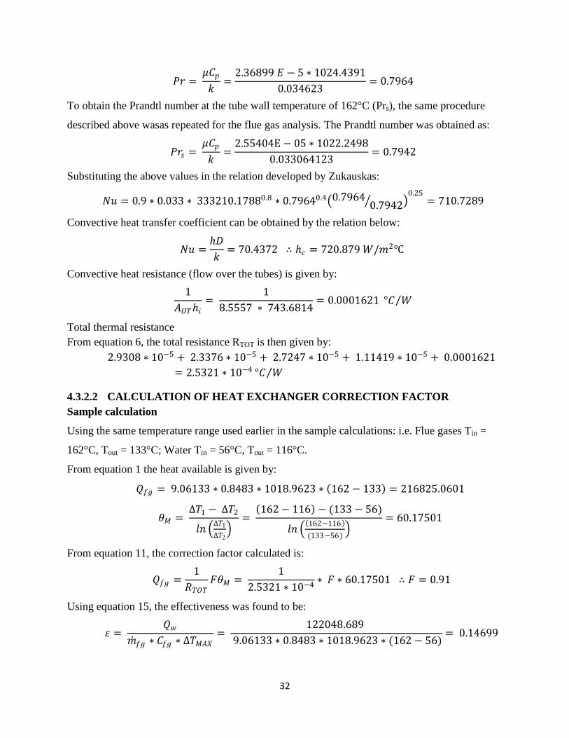
𝑃𝑟 = 𝜇𝐶𝑝
𝑘=
2.36899 𝐸 − 5 ∗ 1024.4391
0.034623= 0.7964
To obtain the Prandtl number at the tube wall temperature of 162°C (Prs), the same procedure
described above wasas repeated for the flue gas analysis. The Prandtl number was obtained as:
𝑃𝑟𝑠 = 𝜇𝐶𝑝
𝑘=
2.55404E − 05 ∗ 1022.2498
0.033064123= 0.7942
Substituting the above values in the relation developed by Zukauskas:
𝑁𝑢 = 0.9 ∗ 0.033 ∗ 333210.17880.8 ∗ 0.79640.4 0.79640.7942
0.25= 710.7289
Convective heat transfer coefficient can be obtained by the relation below:
𝑁𝑢 =𝐷
𝑘= 70.4372 ∴ 𝑐 = 720.879 𝑊/𝑚2℃
Convective heat resistance (flow over the tubes) is given by:
1
𝐴𝑂𝑇𝑖=
1
8.5557 ∗ 743.6814= 0.0001621 °𝐶 𝑊
Total thermal resistance
From equation 6, the total resistance RTOT is then given by:
2.9308 ∗ 10−5 + 2.3376 ∗ 10−5 + 2.7247 ∗ 10−5 + 1.11419 ∗ 10−5 + 0.0001621
= 2.5321 ∗ 10−4 °𝐶 𝑊
4.3.2.2 CALCULATION OF HEAT EXCHANGER CORRECTION FACTOR
Sample calculation
Using the same temperature range used earlier in the sample calculations: i.e. Flue gases Tin =
162°C, Tout = 133°C; Water Tin = 56°C, Tout = 116°C.
From equation 1 the heat available is given by:
𝑄𝑓𝑔 = 9.06133 ∗ 0.8483 ∗ 1018.9623 ∗ 162 − 133 = 216825.0601
𝜃𝑀 = ∆𝑇1 − ∆𝑇2
𝑙𝑛 ∆𝑇1
∆𝑇2
= 162 − 116 − (133 − 56)
𝑙𝑛 162−116
(133−56)
= 60.17501
From equation 11, the correction factor calculated is:
𝑄𝑓𝑔 =1
𝑅𝑇𝑂𝑇𝐹𝜃𝑀 =
1
2.5321 ∗ 10−4∗ 𝐹 ∗ 60.17501 ∴ 𝐹 = 0.91
Using equation 15, the effectiveness was found to be:
𝜀 = 𝑄𝑤
𝑚 𝑓𝑔 ∗ 𝐶𝑓𝑔 ∗ ∆𝑇𝑀𝐴𝑋=
122048.689
9.06133 ∗ 0.8483 ∗ 1018.9623 ∗ (162 − 56)= 0.14699
33
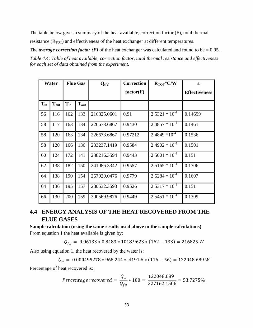
The table below gives a summary of the heat available, correction factor (F), total thermal
resistance (RTOT) and effectiveness of the heat exchanger at different temperatures.
The average correction factor (F) of the heat exchanger was calculated and found to be = 0.95.
Table 4.4: Table of heat available, correction factor, total thermal resistance and effectiveness
for each set of data obtained from the experiment.
Water Flue Gas Q(fg) Correction
factor(F)
RTOT°C/W ε
Effectiveness
Tin Tout Tin Tout
56 116 162 133 216825.0601 0.91 2.5321 * 10-4
0.14699
58 117 163 134 226673.6867 0.9430 2.4857 * 10-4
0.1461
58 120 163 134 226673.6867 0.97212 2.4849 *10-4
0.1536
58 120 166 136 233237.1419 0.9584 2.4902 * 10-4
0.1501
60 124 172 141 238216.3594 0.9443 2.5001 * 10-4
0.151
62 138 182 150 241086.3342 0.9557 2.5165 * 10-4
0.1706
64 138 190 154 267920.0476 0.9779 2.5284 * 10-4
0.1607
64 136 195 157 280532.3593 0.9526 2.5317 * 10-4
0.151
66 130 200 159 300569.9876 0.9449 2.5451 * 10-4
0.1309
4.4 ENERGY ANALYSIS OF THE HEAT RECOVERED FROM THE
FLUE GASES
Sample calculation (using the same results used above in the sample calculations)
From equation 1 the heat available is given by:
𝑄𝑓𝑔 = 9.06133 ∗ 0.8483 ∗ 1018.9623 ∗ 162 − 133 = 216825 𝑊
Also using equation 1, the heat recovered by the water is:
𝑄𝑤 = 0.000495278 ∗ 968.244 ∗ 4191.6 ∗ 116 − 56 = 122048.689 𝑊
Percentage of heat recovered is:
𝑃𝑒𝑟𝑐𝑒𝑛𝑡𝑎𝑔𝑒 𝑟𝑒𝑐𝑜𝑣𝑒𝑟𝑒𝑑 = 𝑄𝑤𝑄𝑓𝑔
∗ 100 = 122048.689
227162.1506= 53.7275%
34
Table 4.5: Table of calculated heat available, heat recovered, ∆Tmax and the percentage of heat
recovered.
4.5 THEORETICAL SIMULATIONS
The theoretical simulation done in this section makes an assumption of steady state operation for
an entry temperature of flue gases of 145 °C and 200 °C.
From the results obtained, and using a correction factor of 0.95 theoretical simulations were done
for the heat recovery unit at inlet flue gas temperatures of Tin = 200°C and Tout = 145°C.
Sample calculation
Water Flue Gas Qfg
Qw
%
Recovered
∆Tmax
Tin Tout Tin Tout
56 116 162 133 216825 122049 56.29 106
58 117 163 134 226674 119934 52.91 105
58 120 163 134 226674 126022 55.6 105
58 120 166 136 233237 126022 54.03 108
60 124 172 141 238216 129990 54.56 112
62 138 182 150 241086 154242 63.98 120
64 138 190 154 267920 150735 56.21 126
64 136 195 157 280532 146039 52.06 131
66 130 200 159 300570 150735 51.4547 134

35
Take the inlet flue gas temperature as Tin = 200 °C and Tout = 145 °C (as stated above) and Tin of
water = 20 °C,
Using a similar flue gas analysis as done in table 4.3 and 4.4 and using a mean bulk temperature
of around 70°C,
From equation 1, the heat available from the flue gas stream is given by:
𝑄𝑓𝑔 = 9.06133 ∗ 0.8007 ∗ 1021.6525 ∗ 200 − 145 = 407721.7097 𝐽/𝑠
From equation 4, the Total thermal resistance is:
𝑅𝑇𝑂𝑇 = 2.4713 ∗ 10−4 °𝐶 𝑊
From equation 2, the overall heat transfer between the two fluids is given by:
𝑄 = 𝑈𝐴𝜃𝐶𝑂𝑅 = 𝜃𝐶𝑂𝑅𝑅𝑇𝑂𝑇
Where θCORR is given as shown in equation 9:
𝜃𝐶𝑂𝑅𝑅 = 𝐹𝜃𝑀
Substituting for Q, F = 0.95, and RTOT = 2.4713 * 10-4°C/W. Using a combination of equation 4
and equation 11,
407721.7097 ∗ 2.4713 ∗ 10−4
0.95 = 𝜃𝑀 = 105.42
Using alteration, from equation 10:
𝜃𝑀 = ∆𝑇1 − ∆𝑇2
𝑙𝑛 ∆𝑇1
∆𝑇2
= 106.06 = 200 − 𝑥 − (145 − 20)
𝑙𝑛 200−𝑥
(145−20)
The value x therefore is obtained as 112°C. From the steam table, the corresponding saturation
pressure is 1.53Bar.
Using equation 1, the Energy gained by the water is given by:
𝑄𝑤 = 0.000495378 ∗ 992.7227 ∗ 4161 ∗ 112 − 20 = 188257 𝐽/𝑠
The percentage of heat recovered may be given as:
% 𝑟𝑒𝑐𝑜𝑣𝑒𝑟𝑒𝑑 = 𝑄𝑤𝑄𝑓𝑔
∗ 100 = 188257
407722∗ 100 = 46.17%
Table 4.6: Table of calculated heat available, heat recovered, percentage of heat recovered and
corresponding Ps values for Tfgin = 200°C

36
Tin
(Water)
T
out(Water)
Qfg
Qw
%
Recovered
20 112 407722 188257 46.17
25 107 407722 167602 41.61
30 104 407722 151131 37.07
35 99 407722 130589 32.03
40 94 407722 110093 27
45 90 407722 91660 22.5
50 84 407722 69202 17
55 78 407722 46777 11.47
60 70 407722 20326 4.99
The corresponding saturation pressures at feed water inlet temperatures of 20 °C and expected
outlet temperature of 112°C(as obtained from alteration) was found to be 1.53 Bar and 1.3 Bar
for a feed water inlet temperature of 25 °C and expected outlet temperature of 107 °C.
In steady state working conditions, it is expected that the flue gas at entry to the heat exchanger
unit is 700 °C with an outlet temperature of 200°C. The flow rate of the flue gases at full
capacity is taken as 24000 cfm (full capacity) and water flow rate taken to be 3m3/hr. Using
equation 1, the total heat available is therefore:
Taking mfg= 5.3297kg/s Cpg= 1.062kJ/Kg.K Tgin=7000C Tgout = 200
0C
𝑄 = 𝑚 𝐶𝑝∆𝑇 = 5.3297 ∗ 1062 ∗ 500 = 2,831,384𝑊
For the water side;
Taking mw=0.8333Kg/s at 250C h1=104.8*10
3 At 130
0 Ch2 =2720*10
3
𝑄 = 𝑚∆ 𝑡 = 0.8333 ∗ 2720 − 104.8 1000 = 2179333.25𝑊
This is 75% of the total energy available.

37
CHAPTER FIVE: DISCUSSION, CONCLUSION AND
RECOMMENDATIONS
5.1 DISCUSSION
A water analysis was done and the total dissolved solids content in the water was found to be
1847.6 mg/l. The proposed method of hardness removal was use of sodium tri- phosphate.The
quantity to be used wascalculated and found to be 88.74g for 1000 liters of water tobetreated.
Use of hydrazine was considered as an oxygen remover but because of it was highly poisonous
nature, Sodium Sulphite was proposed.Sodium Sulphite is very reactive and reduces oxygen
levels to less than 5ppb. The quantity to be used was calculated and found to be 84.6052g for
every 1000liters of water.
The inlet and outlet water temperatures were obtained and recorded in tables. These values
ranged from 560 to66
0 and 116
0 to 138
0 for the inlet and outlet respectively.
From the results obtainedit is observed that the higher the temperature difference between the
flue gas stream at entry and water at entry, the higher the amount of heat recovered.
For optimum heat recovery, the water temperature at entry should be as low as possible. This is
as evidenced by the graph plotted (Appendix B1).After the water temperature at entry reached
62°C, the heat recovered began to decline even with increase in the heat available for recovery
from the flue gas stream. It is also evidenced by the theoretical simulation graphs that were
plotted (Appendix B3) that the heat recovered is high when the inlet water temperature is low.
The inlet temperature increased due reduced efficiency of cooling by the radiator in the pond.
The radiator evaporated contaminated water when the hot water passed through it leaving it
exposed to the air. This reduced the cooling rate and in effect it hadas discussed above in
reducing the heat recovered and also reducing the outlet temperature of the water (see table 4.2).
The highest temperature of water at the outlet attained was 138°C. It then reduced to 136°C and
finally to 130°C.
From the results, it is also seen that the value of thermal resistance increases with increase in
temperature. With the thermal resistance being larger, the reciprocal, decreases (the product of
overall heat transfer coefficient U and surface area A). This leads therefore to a larger amount of

38
heat recovered. Therefore, for more heat to be recovered, the flue gas stream should be at high
temperatures.
From the results obtained, the water did not change phase to steam. However, with proper
lagging of the chimney, the flue gas has an energy potential of about 2.8 Megawatts. From the
analysis above, the flue gas stream can be used to heat water up to saturated steam conditions.
Further provision may be made for a super heater.
5.2 CONCLUSION
The borehole water was analyzed to determine the salts in solution. From the analysis, awater
treatment method was recommended to enable the experimental analysis to be done. This was to
prevent damage of the helical coil heat exchanger by scaling and corrosion (by dissolved
oxygen). The water treatment method chosen involved dosing the water with 88.74 g of Sodium
Triphosphate for every 1000 liters of water and 84.6 g of Sodium Sulphite for every 1000 liters.
The average correction factor (F) of the heat exchanger was calculated and found to be 0.95.
Thermal resistance and effectiveness (ε) at different flue gas and water temperatures were
calculated using the data obtained experimentally. This is as tabulated in table 4.6. The thermal
resistance was seen to increase with increase in temperature.
The most optimum heat that can be recovered was found to be at a very low water inlet
temperature and at a high flue gas temperature. From the theoretical simulation done(without
change in phase), the most optimum heat that can be recovered with an inlet flue gas temperature
of 200 °C, outlet flue gas temperature of 145°C and water inlet temperature of 20 °C was found
to be 188257 J/s.
For an inlet flue gas temperature of 700°C and outlet flue gas temperature of 200 °C , the flue gas
stream has an energy potential of about 2.8 Megawatts that can be harnessed to heat water to
saturated steam conditions at 2.8 Bar.
A Microsoft Excel workbook has been built to aid in further analysis of this project. Screen shots
of the excel workbook are attached in appendix C.
39
5.3 RECOMMENDATIONS
Good working instruments should be installed for proper pressure, temperature and flow rate
readings to facilitate further experimental analysis.
In the flue gas stream, a pitot static pressure gauge should be installed so as to determine the
pressure drop. A CTM-034 flue gas analyzer should also be installed to determine the flue
gas composition.
The chimney should have a thicker lining of insulation installed. A lot of heat is lost in the
upper regions of the chimney stack by radiation and convection.
Further experimental analysis of the heat recovery unit should be done to determine the
optimal mass flow rates of water, flue gases and corresponding temperature values when the
incinerator plant is in steady state operating conditions (i.e. temperatures for both the water
inlet and flue gas inlet are constant). The results obtained were when the incinerator was
working in transient state (the temperatures did not reach a constant value).
For maximum heat recovery and efficiency, the water inlet temperature should be maintained
at low temperatures of about 25°C-30°C. From the analysis done, the lower the inlet
temperature of the water, the higher the heat recovered Qw. It is proposed that a vacuum
surface condenser be designed and installed. It will make use of a water circuit that will be
connected to the radiator in the cooling pond. It is proposed that the radiator in the cooling
pond have its surface area increased to allow a larger area of evaporation and the
contaminated water pool be completely filled with cold water for faster heat loss.
The borehole contains water with a high content of total dissolved solids (1847.6 mg/l). After
further experimental analysis has been done and it has been established that the project is
fully viable for power generation, it is recommended that Reverse Osmosis to be used. This
is the recommended method of feed water treatment for total dissolved solid contents of
greater than 1000 mg/l (see Appendix A2). This treatment is capable of removing up to 99%
of dissolved solids. This will remove the need for further chemical dosing (except oxygen
scavenging) and filming amines in the condenser.
As described earlier, fouling is a general term that includes any kind of deposition of
extraneous material that appears upon the heat transfer surface during the lifetime of the heat
exchanger. Whatever the cause or exact nature of the deposit, an additional resistance to heat
transfer is introduces and the operational capability of the heat exchanger is correspondingly

40
reduced. If fouling cannot be prevented (as it is for our case) it’s necessary to make some
provisions for its periodic removal. By installing a blower that will occasionally blow out the
soot in the heat exchanger, the amount of fouling will be reduced.
Further academic research, further laboratory experiments, analysis and simulations should
be done to determine more Nusselt number relations for flow over helical tubes in different
configurations. Approximations of Nusselt number are done using relations for flow over
tube banks deloped by Zukauskas if the relation is not available for the particular heat
exchanger (like in this case).

41
REFERENCES
TEXT BOOKS
1. Boyen J.L.: Practical Heat Recovery, John Wiley and Sons Inc, Toronto, 1975.
2. BS 2486-1997: Recommendations for treatment of water for steam boilers and water heaters.
3. Cengel Y. A., BolesM. A: Thermodynamics: An Engineering Approach, (5th
Edition),
McGraw-Hill, 2003
4. Luti F.M., University of Nairobi: Notes on Heat Transfer: An Introduction, Lecture notes
2012.
5. Incropera, Bergman D., Lavine: Fundamentals of Heat and Mass Transfer.
6. RayaproluKumar.: Boilers for power and processes, CRC Press, Boca Raton, FL, 2009.
7. Reiter S.: Industrial and Commercial Heat Recovery Systems, Van Nostrand Reinhold
Company New York, 1983.
8. Shar R., Dusan P. S.: Fundamentals of Heat Exchanger Design, John Wiley and Sons Inc,
New Jersey, 2003.
9. GanapathyV.: Industial Boilers and Heat Recovery Steam Generators, Mercel Dekker Inc,
New York 2003.
10. BarasaW.A., S.K. Ngugi: Designing a Boiler Chimney Heat Recovery System against
Fouling, Nairobi, University of Nairobi 2009.
11. CengelY.A.: Heat Transfer: A practical Approach, (2nd
Edition), McGraw-Hill, 2002
12. . Rajput R. K: Heat and Mass Transfer
INTERNET SOURCES
1. Association of Water Technologies, Technical Manual. Accessed from url:
www.steamforum.com/pictures/water%20treat%20boilers(1).pdf on 1st October 2014.
2. Basics of reverse osmosis- Accessed from urlhttp://puretecwater.com/resources/basics-of-
reverse-osmosis.pdf on 1st October 2014.
3. BCS, Incorporated: Waste Heat Recovery: Technology and Opportunities in U.S. Industry,
U.S. Department of Energy, 2008. Accessed from
urlhttp://www1.eere.energy.gov/manufacturing/intensiveprocesses/pdfs/waste_heat_recovery
.pdf on 1st October 2014.
4. Business and Government Energy Management Divison, Department of Energy Mines and
Resources: Waste Heat Recovery, Ottawa. Accessed from url: http://www.em-
42
ea.org/Guide%20Books/book-2/2.8%20Waste%20Heat%20Recovery.pdf on 1st October
2014.
5. Coronel P., Sandeep K.P.: Heat transfer coefficient in Helical Heat Exchangers under
Turbulent Flow conditions. International Journal of Food Engineering Volume 4 Issue 1
Article 4 2008. Doi: 10.2202/1556-3758.1209, January 2008
6. Council of Industrial Boiler Owners (CIBO): Energy Efficiency Handbook, 1997 accessed
from url:
https://www.eere.energy.gov/manufacturing/technical_assistance/pdfs/steamhandbook.pdf on
6th April 2015.
7. Electricity costs in Kenya accessed from urlhttps://stima.regulusweb.com/ on 6th
April 2015
8. Conditional Test Methods (CTM)-034 accessed from
urlwww.epa.gov/ttemc01/ctm.html/ctm-034.pdf on 6th
April 2015.
9. J.M. Hill (2011) Study of Low-Grade Waste Heat Recovery and Energy Transportation
Systems In Industrial Applications (A thesis). Tuscaloosa, University of Alabama. Accessed
from url:
http://acumen.lib.ua.edu/content/u0015/0000001/0000628/u0015_0000001_0000628.pdf on
1st October 2014.
10. Kharat Rahul, Nitin Bhardwaj.: Development of heat transfer coefficient co-relation for
concentric helical coil heat exchanger. International Journal of Thermal Sciences, 48, 2009,
2300-2308. Accessed from url: http://aaqr.org/VOL14_No3_April2014/23_AAQR-13-01-
OA-0028_840-849.pdf on 2nd March 2015.
11. Shi Chang WU, Young Min Jo: Effect of Heat Recovery from flue gas on local humidity and
NOx dispersal in a thermal power station, Taiwan Association for Aerosol Research,doi:
10.4209/aaqr.2013.01.0028, 2013.

43
APPENDICES
APPENDIX A: FEED WATER TREATMENT
Appendix A1: Recommended feed water characteristics for non fired water boilers.
Parameter Unit Recommended
Standard Value
Feed water at economizer inlet
Total hardness mg/kg CaCO3 Not Detectable
pH value at 25°C pH scale 9.3 to 9.8
Oxygen O2 max. mg/l 0.02
Iron and copper and nickel max. mg/l 0.05
Boiler water (Chemicals Added)
Phosphate P04 mg/l 20 to 40
Caustic alkalinity mg/l CaCO3 25 to 50
Silica SiO2 mg/l 20
Oxygen scavenger
Sodium sulfite mg/kg Na2SO3
or
Hydrazine mg/kgN2H4
or
DEHA mg/kg
or
Tannin or
Iso ascorbic acid
mg/l
mg/l
mg/l
15 to 20
0.1 to 0.5
0.1 to 0.25
in feed water
120 to 160
15 to 30
Dissolved solids max mg/kg 1000
Conductivity µS/cm 2000
Table adapted from BS: 2486-1997
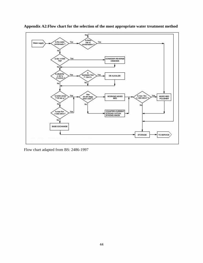
44
Appendix A2:Flow chart for the selection of the most appropriate water treatment method
Flow chart adapted from BS: 2486-1997

45
APPENDIX B: GRAPHS
Appendix B1: Graph showing variation of heat recovered and available with inlet water
temperature
0
50000
100000
150000
200000
250000
300000
350000
54 56 58 60 62 64 66 68
He
at (
J/s)
Inlet Temperature °C
Graph of the heat available and heat recovered against inlet water temperature
Heat available
Heat recovered
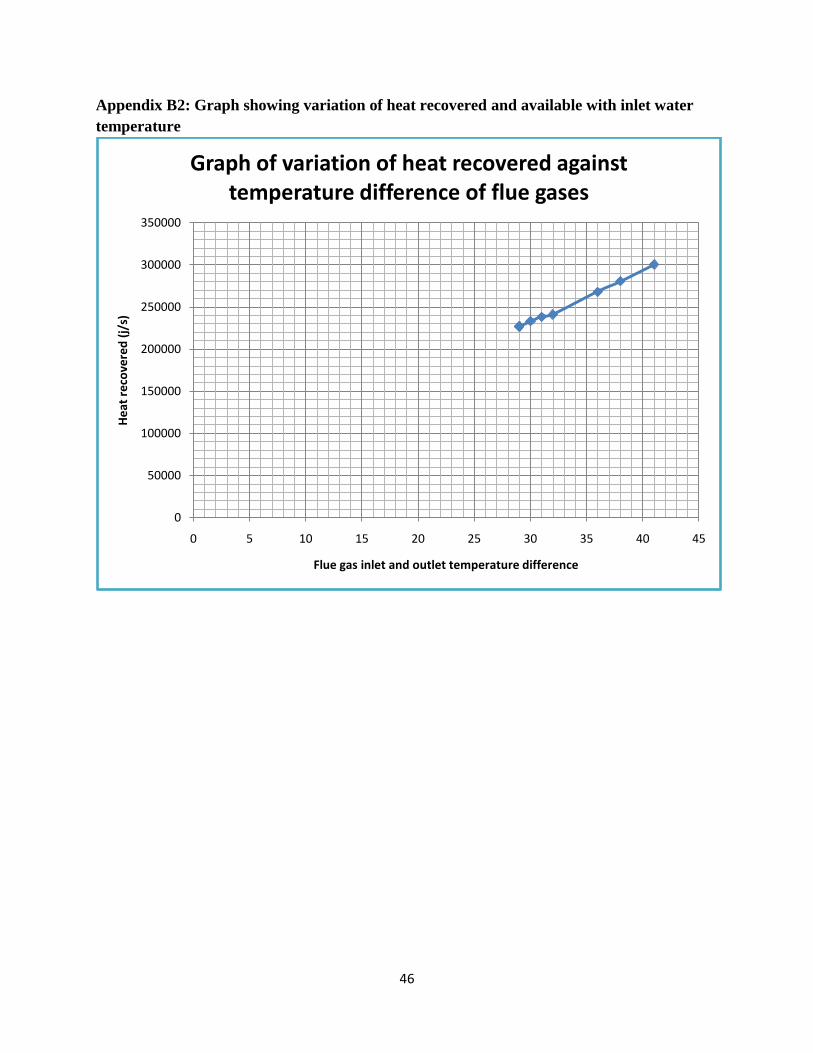
46
Appendix B2: Graph showing variation of heat recovered and available with inlet water
temperature
0
50000
100000
150000
200000
250000
300000
350000
0 5 10 15 20 25 30 35 40 45
He
at r
eco
vere
d (
j/s)
Flue gas inlet and outlet temperature difference
Graph of variation of heat recovered against temperature difference of flue gases

47
Appendix B3: Graph showing the theoretical simulation of variation of heat recovered
against inlet water temperature at Tin = 200°C and Tout = 145°C
0
20000
40000
60000
80000
100000
120000
140000
160000
180000
200000
0 10 20 30 40 50 60 70
He
at R
eco
vere
d (
J/s)
Inlet Temperature °C
Graph of heat recovered against inlet water temperature at flue gas T in = 200 ° C

48
APPENDIX C: MICROSOFT EXCEL WORKBOOK SCREENSHOTS
USED IN THE CALCULATIONS.
Appendix C1: Calculation of the convective heat transfer coefficient of the flue gases and
the corresponding thermal resistance.

49
Appendix C2: Calculation of the convective heat transfer coefficient of the water and the
corresponding thermal resistance.

50
Appendix C3: Calculation of effectiveness, fouling factor, total heat available, total heat
recovered and percentage of heat recovered.
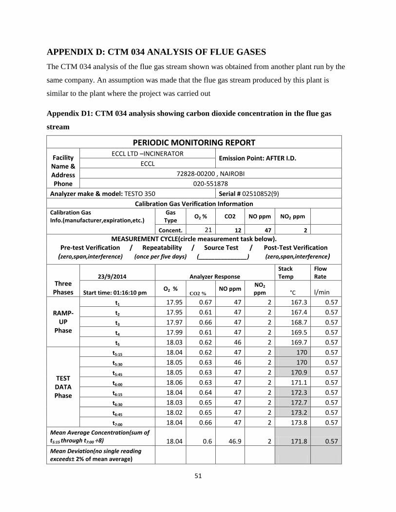
51
APPENDIX D: CTM 034 ANALYSIS OF FLUE GASES
The CTM 034 analysis of the flue gas stream shown was obtained from another plant run by the
same company. An assumption was made that the flue gas stream produced by this plant is
similar to the plant where the project was carried out
Appendix D1: CTM 034 analysis showing carbon dioxide concentration in the flue gas
stream
PERIODIC MONITORING REPORT
Facility Name & Address Phone
ECCL LTD –INCINERATOR Emission Point: AFTER I.D.
ECCL
72828-00200 , NAIROBI
020-551878
Analyzer make & model: TESTO 350 Serial # 02510852(9)
Calibration Gas Verification Information Calibration Gas Info.(manufacturer,expiration,etc.)
Gas Type
O2 % CO2 NO ppm NO2 ppm
Concent. 21 12 47 2
MEASUREMENT CYCLE(circle measurement task below). Pre-test Verification / Repeatability / Source Test / Post-Test Verification
(zero,span,interference) (once per five days) (_______________) (zero,span,interference)
Three Phases
23/9/2014 Analyzer Response Stack Temp
Flow Rate
Start time: 01:16:10 pm O2 %
CO2 % NO ppm
NO2 ppm °C l/min
RAMP-UP
Phase
t1 17.95 0.67 47 2 167.3 0.57
t2 17.95 0.61 47 2 167.4 0.57
t3 17.97 0.66 47 2 168.7 0.57
t4 17.99 0.61 47 2 169.5 0.57
t5 18.03 0.62 46 2 169.7 0.57
TEST DATA Phase
t5:15 18.04 0.62 47 2 170 0.57
t5:30 18.05 0.63 46 2 170 0.57
t5:45 18.05 0.63 47 2 170.9 0.57
t6:00 18.06 0.63 47 2 171.1 0.57
t6:15 18.04 0.64 47 2 172.3 0.57
t6:30 18.03 0.65 47 2 172.7 0.57
t6:45 18.02 0.65 47 2 173.2 0.57
t7:00 18.04 0.66 47 2 173.8 0.57
Mean Average Concentration(sum of t5:15 through t7:00 ÷8) 18.04 0.6 46.9 2 171.8 0.57
Mean Deviation(no single reading exceeds± 2% of mean average)

52
Acceptable "Test Data Phase" Yes or No
Yes or No
Yes or No
Yes or No
REFRESH Phase
t7 18.06 0.65 46 2 173.9 0.57
t8 18.07 0.66 45 2 174.1 0.57
t9 18.07 0.65 45 2 174.1 0.57
t10 18.06 0.66 45 2 174.6 0.57
t11 18.05 0.66 45 2 175 0.57
t12 18.03 0.65 45 2 175.4 0.57
t13 18.03 0.65 46 2 175.5 0.57
t14 17.98 0.64 46 2 175.5 0.57
t15 17.95 0.64 48 2 176.1 0.57
Stop Time : 1:16:39 pm
Appendix D2: CTM 034 analysis showing carbon monoxide concentration in flue gas
stream
PERIODIC MONITORING REPORT
Facility Name & Address Phone
ECCL LTD -INCINERATOR Emission Point: AFTER I.D.
ECCL
72828-00200 , NAIROBI
020-551878
Analyzer make & model: TESTO 350 Serial # 02510852(9)
Calibration Gas Verification Information Calibration Gas Info.(manufacturer,expiration,etc.)
Gas Type O2 % CO ppm NO ppm NO2 ppm
Concent.
MEASUREMENT CYCLE(circle measurement task below). Pre-test Verification / Repeatability / Source Test / Post-Test Verification
(zero,span,interference) (once per five days) (_______________) (zero,span,interference)
Three Phases
23/9/2014 Analyzer Response Stack Temp
Flow Rate
Start time: 01:16:10 pm O2 % CO ppm NO ppm
NO2 ppm °C l/min
RAMP-UP
Phase
t1 17.95 60 47 2 167.3 0.57
t2 17.95 60 47 2 167.4 0.57
t3 17.97 61 47 2 168.7 0.57
t4 17.99 61 47 2 169.5 0.57
t5 18.03 62 46 2 169.7 0.57
TEST DATA Phase
t5:15 18.04 62 47 2 170 0.57
t5:30 18.05 62 46 2 170 0.57
t5:45 18.05 63 47 2 170.9 0.57
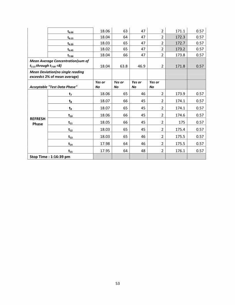
53
t6:00 18.06 63 47 2 171.1 0.57
t6:15 18.04 64 47 2 172.3 0.57
t6:30 18.03 65 47 2 172.7 0.57
t6:45 18.02 65 47 2 173.2 0.57
t7:00 18.04 66 47 2 173.8 0.57
Mean Average Concentration(sum of t5:15 through t7:00 ÷8) 18.04 63.8 46.9 2 171.8 0.57
Mean Deviation(no single reading exceeds± 2% of mean average)
Acceptable "Test Data Phase" Yes or No
Yes or No
Yes or No
Yes or No
REFRESH Phase
t7 18.06 65 46 2 173.9 0.57
t8 18.07 66 45 2 174.1 0.57
t9 18.07 65 45 2 174.1 0.57
t10 18.06 66 45 2 174.6 0.57
t11 18.05 66 45 2 175 0.57
t12 18.03 65 45 2 175.4 0.57
t13 18.03 65 46 2 175.5 0.57
t14 17.98 64 46 2 175.5 0.57
t15 17.95 64 48 2 176.1 0.57
Stop Time : 1:16:39 pm
Recommended