Program Analysis and Synthesis of Parallel Systems
Roman Manevich Ben-Gurion University

Three papers
1. A Shape Analysis for Optimizing Parallel Graph Programs [POPL’11]
2. Elixir: a System for Synthesizing Concurrent Graph Programs [OOPSLA’12]
3. Parameterized Verification of Transactional Memories [PLDI’10]

What’s the connection?
A Shape Analysisfor Optimizing ParallelGraph Programs [POPL’11]
Elixir: a System for SynthesizingConcurrent Graph Programs [OOPSLA’12]
Parameterized Verificationof Transactional Memories [PLDI’10]
From analysisto language design
Creates opportunitiesfor more optimizations.Requires other analyses
Similarities betweenabstract domains

A Shape Analysis for Optimizing Parallel Graph Programs
Dimitrios Prountzos1
Keshav Pingali1,2
Roman Manevich2
Kathryn S. McKinley1
1: Department of Computer Science, The University of Texas at Austin2: Institute for Computational Engineering and Sciences, The
University of Texas at Austin

6
Motivation• Graph algorithms are ubiquitous
• Goal: Compiler analysis for optimization of parallel graph algorithms
Computational biology Social Networks
Computer Graphics

7
Minimum Spanning Tree Problem
c d
a b
e f
g
2 4
6
5
3
7
4
1

8
Minimum Spanning Tree Problem
c d
a b
e f
g
2 4
6
5
3
7
4
1

9
Boruvka’s Minimum Spanning Tree Algorithm
Build MST bottom-uprepeat { pick arbitrary node ‘a’ merge with lightest neighbor ‘lt’ add edge ‘a-lt’ to MST} until graph is a single node
c d
a b
e f
g
2 4
6
5
3
7
4
1d
a,c b
e f
g
4
6
3
4
17
lt

10
Parallelism in Boruvka
c d
a b
e f
g
2 4
6
5
3
7
4
1
Build MST bottom-uprepeat { pick arbitrary node ‘a’ merge with lightest neighbor ‘lt’ add edge ‘a-lt’ to MST} until graph is a single node

11
Non-conflicting iterations
c d
a b
2
5
3
7
4
1
Build MST bottom-uprepeat { pick arbitrary node ‘a’ merge with lightest neighbor ‘lt’ add edge ‘a-lt’ to MST} until graph is a single node
e f
g
4
6

12
Non-conflicting iterations
Build MST bottom-uprepeat { pick arbitrary node ‘a’ merge with lightest neighbor ‘lt’ add edge ‘a-lt’ to MST} until graph is a single node
d
a,c b3
4
17
e f,g6

13
Conflicting iterations
c d
a b
e f
g
2 4
6
5
3
7
4
1
Build MST bottom-uprepeat { pick arbitrary node ‘a’ merge with lightest neighbor ‘lt’ add edge ‘a-lt’ to MST} until graph is a single node

Optimistic parallelization in Galois• Programming model
– Client code has sequential semantics– Library of concurrent data structures
• Parallel execution model– Thread-level speculation (TLS)– Activities executed speculatively
• Conflict detection– Each node/edge has associated exclusive
lock– Graph operations acquire locks on
read/written nodes/edges– Lock owned by another thread conflict
iteration rolled back– All locks released at the end
• Two main overheads– Locking– Undo actions
i1
i2
i3

Generic optimization structure
Program AnnotatedProgram
ProgramAnalyzer
ProgramTransformer
OptimizedProgram

Overheads (I): locking• Optimizations– Redundant locking elimination– Lock removal for iteration private data– Lock removal for lock domination
• ACQ(P): set of definitely acquired locks per program point P• Given method call M at P:
Locks(M) ACQ(P) Redundant Locking

18
Overheads (II): undo actions
Lockset Grows
Lockset Stable
Failsafe
…
foreach (Node a : wl) {
…
…
}
foreach (Node a : wl) { Set<Node> aNghbrs = g.neighbors(a); Node lt = null; for (Node n : aNghbrs) { minW,lt = minWeightEdge((a,lt), (a,n)); } g.removeEdge(a, lt); Set<Node> ltNghbrs = g.neighbors(lt); for (Node n : ltNghbrs) { Edge e = g.getEdge(lt, n); Weight w = g.getEdgeData(e); Edge an = g.getEdge(a, n); if (an != null) { Weight wan = g.getEdgeData(an); if (wan.compareTo(w) < 0) w = wan; g.setEdgeData(an, w); } else { g.addEdge(a, n, w); } } g.removeNode(lt); mst.add(minW); wl.add(a);}
Program point P is failsafe if: Q : Reaches(P,Q) Locks(Q) ACQ(P)

GSet<Node> wl = new GSet<Node>();wl.addAll(g.getNodes());GBag<Weight> mst = new GBag<Weight>();
foreach (Node a : wl) { Set<Node> aNghbrs = g.neighbors(a); Node lt = null; for (Node n : aNghbrs) { minW,lt = minWeightEdge((a,lt), (a,n)); } g.removeEdge(a, lt); Set<Node> ltNghbrs = g.neighbors(lt); for (Node n : ltNghbrs) { Edge e = g.getEdge(lt, n); Weight w = g.getEdgeData(e); Edge an = g.getEdge(a, n); if (an != null) { Weight wan = g.getEdgeData(an); if (wan.compareTo(w) < 0) w = wan; g.setEdgeData(an, w); } else { g.addEdge(a, n, w); } } g.removeNode(lt); mst.add(minW); wl.add(a);}
Lockset analysis
• Redundant Locking• Locks(M) ACQ(P)
• Undo elimination• Q : Reaches(P,Q)
Locks(Q) ACQ(P)
• Need to compute ACQ(P)
: Runtime overhead

The optimization technically
• Each graph method m(arg1,…,argk, flag) contains optimization level flag• flag=LOCK – acquire locks • flag=UNDO – log undo (backup) data• flag=LOCK_UNO D – (default) acquire locks and
log undo• flag=NONE – no extra work
• Example:Edge e = g.getEdge(lt, n, NONE)

Analysis challenges
• The usual suspects: – Unbounded Memory Undecidability – Aliasing, Destructive updates
• Specific challenges:– Complex ADTs: unstructured graphs– Heap objects are locked– Adapt abstraction to ADTs
• We use Abstract Interpretation [CC’77]– Balance precision and realistic performance

Shape analysis overview
HashMap-Graph
Tree-based Set
……
Graph { @rep nodes @rep edges …}
Graph Spec
Concrete ADTImplementationsin Galois library
Predicate Discovery
Shape Analysis
Boruvka.javaOptimizedBoruvka.java
Set { @rep cont …}
Set Spec
ADT Specifications

ADT specification
Graph<ND,ED> {
@rep set<Node> nodes @rep set<Edge> edges
Set<Node> neighbors(Node n);
}
Graph Spec
...Set<Node> S1 = g.neighbors(n);
...
Boruvka.java
Abstract ADT state by virtual set fields
@locks(n + n.rev(src) + n.rev(src).dst + n.rev(dst) + n.rev(dst).src)@op( nghbrs = n.rev(src).dst + n.rev(dst).src , ret = new Set<Node<ND>>(cont=nghbrs) )
Assumption: Implementation satisfies Spec

Graph<ND,ED> {
@rep set<Node> nodes@rep set<Edge> edges
@locks(n + n.rev(src) + n.rev(src).dst + n.rev(dst) + n.rev(dst).src)@op( nghbrs = n.rev(src).dst + n.rev(dst).src , ret = new Set<Node<ND>>(cont=nghbrs) ) Set<Node> neighbors(Node n);}
Modeling ADTs
c
a bGraph Spec
dst
src
srcdst
dst
src

Modeling ADTs
c
a b
nodes edges
Abstract State
cont
ret nghbrs
Graph Spec
dst
src
srcdst
dst
src
Graph<ND,ED> {
@rep set<Node> nodes@rep set<Edge> edges
@locks(n + n.rev(src) + n.rev(src).dst + n.rev(dst) + n.rev(dst).src)@op( nghbrs = n.rev(src).dst + n.rev(dst).src , ret = new Set<Node<ND>>(cont=nghbrs) ) Set<Node> neighbors(Node n);}

Abstraction scheme
cont cont
S1 S2L(S1.cont) L(S2.cont)
(S1 ≠ S2) ∧ L(S1.cont) ∧ L(S2.cont)
• Parameterized by set of LockPaths: L(Path) o . o ∊ Path Locked(o)– Tracks subset of must-be-locked objects
• Abstract domain elements have the form: Aliasing-configs 2LockPaths …

27
( L(y.nd) ) )( ( L(x.nd))
( L(y.nd) ) ( L(y.nd) L(x.rev(src)) ) )( ( L(x.nd))
Joining abstract states
( L(y.nd) ) ( () L(x.nd) )
Aliasing is crucial for precisionMay-be-locked does not enable our optimizations
#Aliasing-configs : small constant (6)

28
lt
GSet<Node> wl = new GSet<Node>();wl.addAll(g.getNodes());GBag<Weight> mst = new GBag<Weight>();
foreach (Node a : wl) { Set<Node> aNghbrs = g.neighbors(a); Node lt = null; for (Node n : aNghbrs) { minW,lt = minWeightEdge((a,lt), (a,n)); } g.removeEdge(a, lt); Set<Node> ltNghbrs = g.neighbors(lt); for (Node n : ltNghbrs) { Edge e = g.getEdge(lt, n); Weight w = g.getEdgeData(e); Edge an = g.getEdge(a, n); if (an != null) { Weight wan = g.getEdgeData(an); if (wan.compareTo(w) < 0) w = wan; g.setEdgeData(an, w); } else { g.addEdge(a, n, w); } } g.removeNode(lt); mst.add(minW); wl.add(a);}
Example invariant in Boruvka The immediate neighbors of a and lt are locked
a
( a ≠ lt ) ∧ L(a) L(a.rev(src)) L(a.rev(dst))∧ ∧ ∧ L(a.rev(src).dst) L(a.rev(dst).src) ∧ ∧ L(lt) L(lt.rev(dst)) L(lt.rev(src)) ∧ ∧ ∧ L(lt.rev(dst).src) L(lt.rev(src).dst)∧
…..

Heuristics for finding LockPaths
• Hierarchy Summarization (HS)– x.( fld )*– Type hierarchy graph acyclic
bounded number of paths
– Preflow-Push: • L(S.cont) L(S.cont.nd)∧• Nodes in set S and their data are locked
Set<Node>
S
Node
NodeData
cont
nd

30
Footprint graph heuristic
• Footprint Graphs (FG)[Calcagno et al. SAS’07]– All acyclic paths from arguments of ADT method to locked
objects– x.( fld | rev(fld) )* – Delaunay Mesh Refinement: L(S.cont) L(S.cont.rev(src)) L(S.cont.rev(dst)) ∧ ∧ ∧ L(S.cont.rev(src).dst) L(S.cont.rev(dst).src)∧– Nodes in set S and all of their immediate neighbors
are locked
• Composition of HS, FG– Preflow-Push: L(a.rev(src).ed)FG HS

Experimental evaluation• Implement on top of TVLA– Encode abstraction by 3-Valued Shape Analysis
[SRW TOPLAS’02]• Evaluation on 4 Lonestar Java benchmarks
• Inferred all available optimizations• # abstract states practically linear in program size
Benchmark Analysis Time (sec)
Boruvka MST 6Preflow-Push Maxflow 7Survey Propagation 12Delaunay Mesh Refinement 16

Impact of optimizations for 8 threads
Boruvka MST Delaunay Mesh Refinement
Survey Propaga-tion
Preflow-Push Maxflow
0
50
100
150
200
250
Baseline Optimized
Tim
e (s
ec)
5.6× 4.7×11.4×
2.9× 8-core Intel Xeon @ 3.00 GHz

Note 1
• How to map abstract domain presented so far to TVLA?– Example invariant: (x≠y L(y.nd)) (x=y L(x.nd))– Unary abstraction predicate x(v) for pointer x– Unary non-abstraction predicate
L[x.p] for pointer x and path p– Use partial join– Resulting abstraction similar to the one shown

Note 2
• How to come up with abstraction for similar problems?1. Start by constructing a manual proof• Hoare Logic
2. Examine resulting invariants and generalize into a language of formulas• May need to be further specialized for a given
program – interesting problem (machine learning/refinement)
– How to get sound transformers?

Note 3
• How did we avoid considering all interleavings?
• Proved non-interference side theorem

Elixir : A System for Synthesizing Concurrent Graph Programs
Dimitrios Prountzos1
Roman Manevich2
Keshav Pingali1
1. The University of Texas at Austin2. Ben-Gurion University of the Negev

GoalAllow programmer to easily implement
correct and efficientparallel graph algorithms
• Graph algorithms are ubiquitousSocial network analysis, Computer graphics, Machine learning, …
• Difficult to parallelize due to their irregular nature
• Best algorithm and implementation usually
– Platform dependent– Input dependent
• Need to easily experiment with different solutions• Focus: Fixed graph structure
• Only change labels on nodes and edges• Each activity touches a fixed number of nodes

• Problem Formulation– Compute shortest distance
from source node S to every other node• Many algorithms
– Bellman-Ford (1957)– Dijkstra (1959)– Chaotic relaxation (Miranker 1969)– Delta-stepping (Meyer et al. 1998)
• Common structure– Each node has label dist
with known shortest distance from S• Key operation
– relax-edge(u,v)
Example: Single-Source Shortest-Path
2 5
1 7
A B
C
D E
F
G
S
34
22
1
9
12
2 A
C
3
if dist(A) + WAC < dist(C) dist(C) = dist(A) + WAC

Scheduling of relaxations:• Use priority queue of nodes,
ordered by label dist• Iterate over nodes u in priority
order• On each step: relax all
neighbors v of u – Apply relax-edge to all (u,v)
Dijkstra’s algorithm2 5
1 7
A B
C
D E
F
G
S
34
22
1
9
7
53
6
<C,3> <B,5><B,5> <E,6> <D,7><B,5>

40
Chaotic relaxation
• Scheduling of relaxations:• Use unordered set of edges• Iterate over edges (u,v) in
any order• On each step:– Apply relax-edge to edge (u,v)
2 5
1 7
A B
C
D E
F
G
S
34
22
1
9
5
12
(S,A)(B,C)
(C,D)(C,E)

Insights behind Elixir
What should be done How it should
be done
Unordered/Ordered algorithms
Operator Delta
: activity
Parallel Graph Algorithm
Operators Schedule
Order activity processing
Identify new activities
Static Schedule
Dynamic Schedule
“TAO of parallelism”PLDI 2011

Insights behind ElixirParallel Graph
Algorithm
Operators Schedule
Order activity processing
Identify new activities
Static Schedule
Dynamic Schedule
Dijkstra-style Algorithm
q = new PrQueueq.enqueue(SRC)
while (! q.empty ){ a = q.dequeue
for each e = (a,b,w){ if dist(a) + w < dist(b){
dist(b) = dist(a) + w q.enqueue(b)
} } }
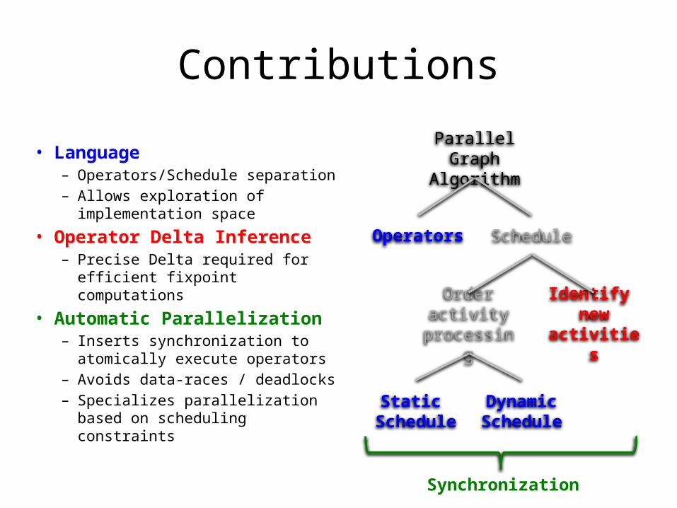
Contributions
• Language– Operators/Schedule separation– Allows exploration of
implementation space
• Operator Delta Inference– Precise Delta required for efficient
fixpoint computations
• Automatic Parallelization– Inserts synchronization to
atomically execute operators– Avoids data-races / deadlocks– Specializes parallelization based on
scheduling constraints
Parallel Graph Algorithm
Operators Schedule
Order activity processing
Identify new activities
Static Schedule
Dynamic Schedule
Synchronization

44
SSSP in Elixir
Graph [ nodes(node : Node, dist : int) edges(src : Node, dst : Node, wt : int)]
relax = [ nodes(node a, dist ad) nodes(node b, dist bd)
edges(src a, dst b, wt w) bd > ad + w ] ➔ [ bd = ad + w ]
sssp = iterate relax schedule≫
Graph type
Operator
FixpointStatement

Operators
Graph [ nodes(node : Node, dist : int) edges(src : Node, dst : Node, wt : int)]
relax = [ nodes(node a, dist ad) nodes(node b, dist bd) edges(src a, dst b, wt w) bd > ad + w ] ➔ [ bd = ad + w ]
sssp = iterate relax schedule ≫
Redex pattern
GuardUpdate
ba if bd > ad + w
adw
bd
ba
adw
ad+w
Cautiousby construction – easy to generalize

46
Fixpoint statement
Graph [ nodes(node : Node, dist : int) edges(src : Node, dst : Node, wt : int)]
relax = [ nodes(node a, dist ad) nodes(node b, dist bd) edges(src a, dst b, wt w) bd > ad + w ] ➔ [ bd = ad + w ]
sssp = iterate relax schedule ≫
Apply operator until fixpoint
Scheduling expression

Scheduling examples
Graph [ nodes(node : Node, dist : int) edges(src : Node, dst : Node, wt : int)]
relax = [ nodes(node a, dist ad) nodes(node b, dist bd) edges(src a, dst b, wt w) bd > ad + w ] ➔ [ bd = ad + w ]
sssp = iterate relax schedule ≫
Locality enhanced Label-correctinggroup b unroll 2 approx metric ad ≫ ≫Dijkstra-style
metric ad group b ≫
q = new PrQueueq.enqueue(SRC)while (! q.empty ) { a = q.dequeue for each e = (a,b,w) { if dist(a) + w < dist(b) { dist(b) = dist(a) + w q.enqueue(b) } }}

Operator Delta Inference
Parallel Graph Algorithm
Operators Schedule
Order activity processing
Identify new activities
Static Schedule
Dynamic Schedule

Identifying the delta of an operator
b
a
relax1
??

Delta Inference Example
ba
SMT Solver
SMT Solver
assume (da + w1 < db)
assume ¬(dc + w2 < db)
db_post = da + w1
assert ¬(dc + w2 < db_post)Query Program
relax1
c
w2
w1
relax2
(c,b) does not become active

assume (da + w1 < db)
assume ¬(db + w2 < dc)
db_post = da + w1
assert ¬(db_post + w2 < dc)Query Program
Delta inference example – active
SMT Solver
SMT Solver
ba
relax1
cw1
relax2
w2
Apply relax on all outgoing edges (b,c) such that:
dc > db +w2
and c a≄

Influence patterns
b=cad
ba=c
d
a=dc
b
b=da=c b=ca=d
b=da
c

System architecture
Elixir
Galois/OpenMP Parallel Runtime
Algorithm Spec
Parallel Thread-PoolGraph ImplementationsWorklist Implementations
Synthesize codeInsert synchronization
C++Program

ExperimentsExplored Dimensions
Grouping Statically group multiple instances of operator
Unrolling Statically unroll operator applications by factor K
Dynamic Scheduler Choose different policy/implementation for the dynamic worklist
...
Compare against hand-written parallel implementations

SSSP results
1 2 4 8 16 20 240
100
200
300
400
500
600
700
800
Elixir
Lonestar
Threads
Tim
e (m
s)
• 24 core Intel Xeon @ 2 GHz• USA Florida Road Network (1 M nodes, 2.7 M Edges)
Group + Unroll improve localityImplementation Variant

Breadth-First search results
Scale-Free Graph1 M nodes, 8 M edges
USA road network24 M nodes, 58 M edges
1 2 4 8 16 20 240
100
200
300
400
500
600
700
800
900
1000
Elixir (Variant 1)LonestarCilk
Threads
Tim
e (m
s)
1 2 4 8 16 20 240
1000
2000
3000
4000
5000
6000
7000
Elixir (Variant 2)LonestarCilk
Threads
Tim
e (m
s)

Conclusion
• Graph algorithm = Operators + Schedule– Elixir language :
imperative operators + declarative schedule• Allows exploring implementation space• Automated reasoning for efficiently computing
fixpoints• Correct-by-construction parallelization • Performance competitive with hand-
parallelized code

Parameterized Verificationof Software Transactional Memories
Michael Emmi Rupak MajumdarRoman Manevich

Motivation
• Transactional memories [Herlihy ‘93]– Programmer writes code w. coarse-grained atomic blocks – Transaction manager takes care of conflicts providing illusion
of sequential execution• Strict serializability – correctness criterion
– Formalizes “illusion of sequential execution”• Parameterized verification
– Formal proof for given implementation– For every number of threads– For every number of memory objects– For every number and length of transactions
59
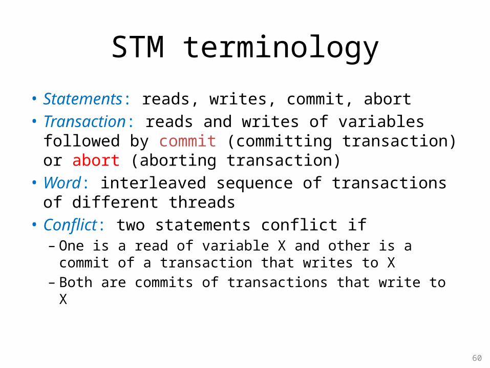
STM terminology
• Statements: reads, writes, commit, abort• Transaction: reads and writes of variables followed
by commit (committing transaction)or abort (aborting transaction)
• Word: interleaved sequence of transactions of different threads
• Conflict: two statements conflict if– One is a read of variable X and other is a commit of a
transaction that writes to X– Both are commits of transactions that write to X
60

Safety property: strict serializability
• There is a serialization for the committing threads such that order of conflicts is preserved
• Order of non-overlapping transactions remains the same
61

Safety property: strict serializability
• There is a serialization for the committing threads such that order of conflicts is preserved
• Order of non-overlapping transactions remains the same• Example word: (rd X t1), (rd Y t2), (wr X t2), (commit t2), (commit t1)
=>
Can be serialized to : (rd X t1), (commit t1), (rd Y t2), (wr X t2), (commit t2)
conflict
conflict62
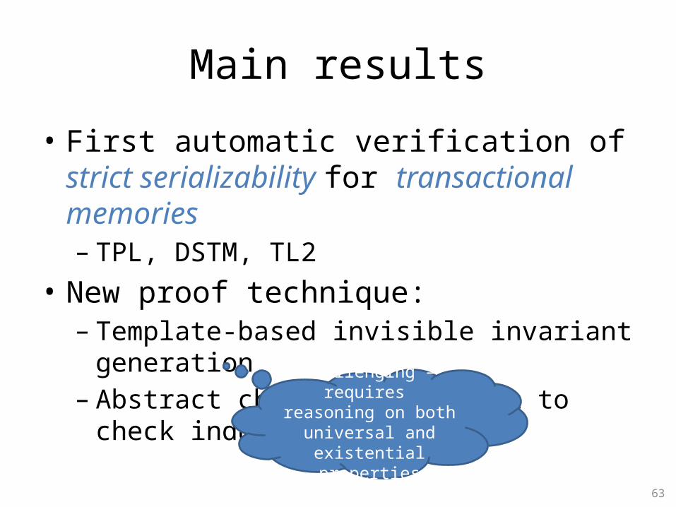
Main results
• First automatic verification ofstrict serializability for transactional memories– TPL, DSTM, TL2
• New proof technique:– Template-based invisible invariant generation– Abstract checking algorithm to check inductive
invariants
63
Challenging – requires reasoning on both
universal and existential properties

Outline
• Strict serializability verification approach• Automating the proof• Experiments• Conclusion• Related work
64

Proof roadmap 1
Goal: prove model M is strictly serializable1. Given a strict-serializability reference model
RSS reduce checking strict-serializabilityto checking that M refines RSS
2. Reduce refinement to checking safety– Safety property SIM: whenever M can execute a
statement so can RSS– Check SIM on product system M RSS
65

Proof roadmap 2
3. Model STMs M and RSS in first-order logic• TM models use set data structures and typestate bits
4. Check safety by generating strong enough candidate inductive invariant and checking inductiveness– Use observations on structure of transactional
memories– Use sound first-order reasoning
66

Reference strict serializability model
• Guerraoui, Singh, Henzinger, Jobstmann [PLDI’08]• RSS : Most liberal specification of strictly
serializable system– Allows largest language of strictly-serializable
executions• M is strictly serializable iff every word of M is also
a word of RSS– Language(M) Language(RSS)– M refines RSS
67
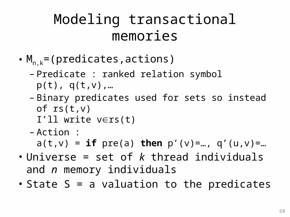
Modeling transactional memories
• Mn,k=(predicates,actions)– Predicate : ranked relation symbol
p(t), q(t,v),…– Binary predicates used for sets so instead of rs(t,v)
I’ll write vrs(t)– Action :
a(t,v) = if pre(a) then p’(v)=…, q’(u,v)=…• Universe = set of k thread individuals and n
memory individuals• State S = a valuation to the predicates
68
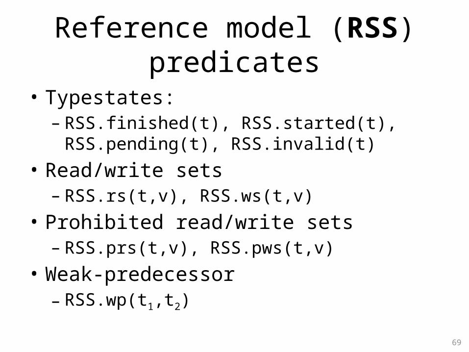
Reference model (RSS) predicates
• Typestates:– RSS.finished(t), RSS.started(t), RSS.pending(t),
RSS.invalid(t)• Read/write sets– RSS.rs(t,v), RSS.ws(t,v)
• Prohibited read/write sets– RSS.prs(t,v), RSS.pws(t,v)
• Weak-predecessor– RSS.wp(t1,t2)
69
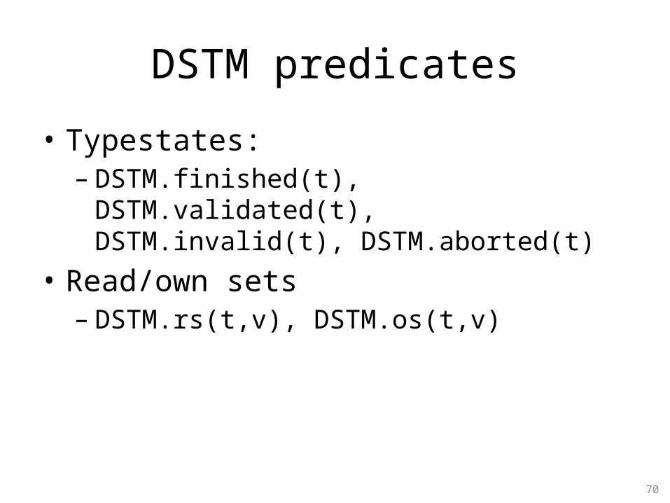
DSTM predicates
• Typestates:– DSTM.finished(t), DSTM.validated(t),
DSTM.invalid(t), DSTM.aborted(t)• Read/own sets– DSTM.rs(t,v), DSTM.os(t,v)
70

RSS commit(t) action
71
if RSS.invalid(t) RSS.wp(t,t) thent1,t2 . RSS.wp’(t1,t2) t1t t2t (RSS.wp(t1,t2) RSS.wp(t,t2) (RSS.wp(t1,t) v . vRSS.ws(t1) vRSS.ws(t)))…
post-statepredicate
current-statepredicate
action precondition
write-write conflict
executing thread

DSTM commit(t) action
if DSTM.validated(t) thent1 . DSTM.validated’(t1) t1t DSTM.validated(t1) v . vDSTM.rs(t1) vDSTM.os(t1)…
72
read-own conflict
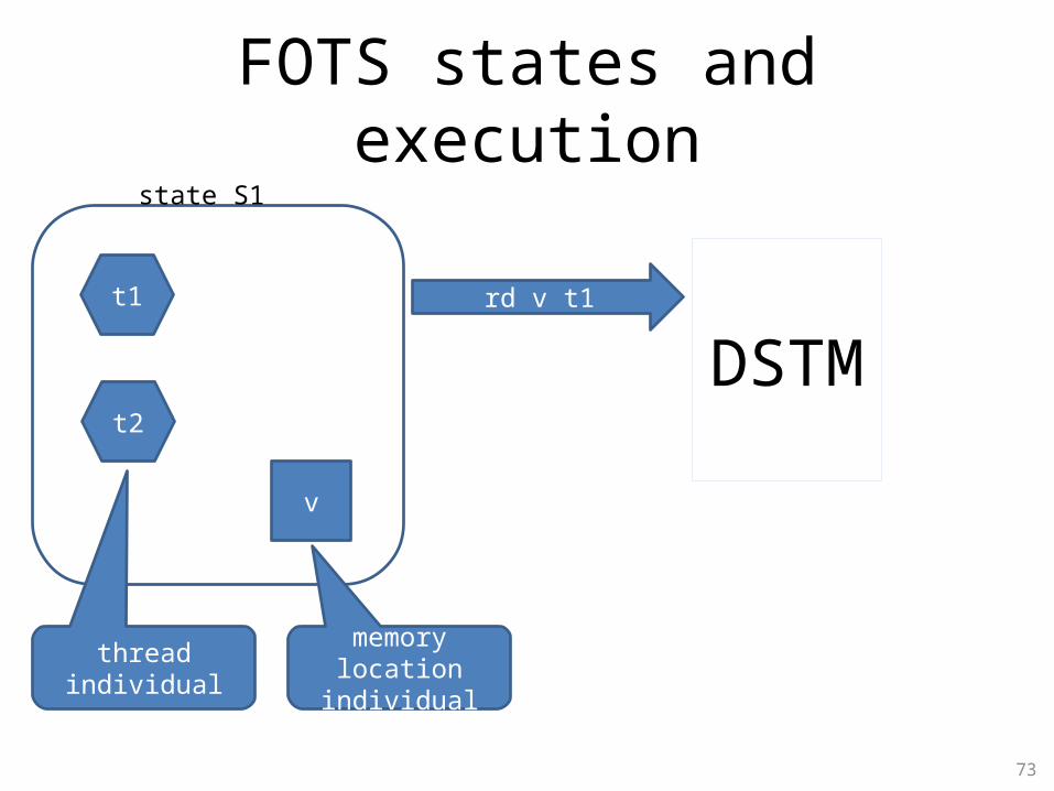
FOTS states and execution
v
rd v t1
DSTMt1
t2
73
memory locationindividual
threadindividual
state S1

FOTS states and execution
v
rd v t1
DSTM.rs
predicate evaluationDSTM.rs(t1,v)=1
DSTMt1
t2
DSTM.started
74
predicate evaluationDSTM.started(t1)=1
state S2

FOTS states and execution
v
wr v t2
DSTM.rs DSTMt1
t2 DSTM.ws
DSTM.started
DSTM.started
75
state S3

Product system
• The product of two systems: AB • Predicates = A.predicates B.predicates• Actions =
commit(t) = { if (A.pre B.pre) then … }rd(t,v) = { if (A.pre B.pre) then … }…
• M refines RSS iff on every executionSIM holds: action a M.pre(a) RSS.pre(a)
76

Checking DSTM refines RSS
• The only precondition in RSS is for commit(t)• We need to check SIM =
t.DSTM.validated(t) RSS.invalid(t) RSS.wp(t,t) holds for DSTM RSS for all reachable states
• Proof rule:
77
DSTMRSS SIM
DSTM refines RSS
how do we check this safety
property?
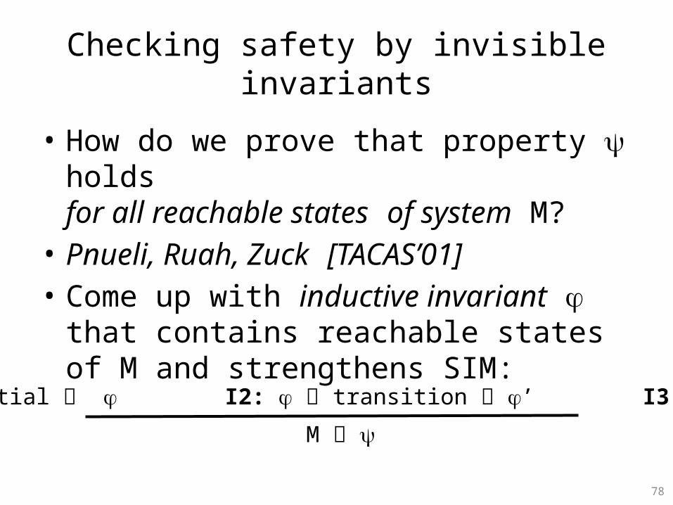
Checking safety by invisible invariants
• How do we prove that property holdsfor all reachable states of system M?
• Pnueli, Ruah, Zuck [TACAS’01]• Come up with inductive invariant that
contains reachable states of M and strengthens SIM:
78
I1: Initial I2: transition ’ I3:
M

Strict serializability proof rule
Proof roadmap:1. Divine candidate invariant 2. Prove I1, I2, I3
I1: Initial I2: transition ’ I3: SIM
DSTM RSS SIM
79

Two challenges
Proof roadmap:1. Divine candidate invariant 2. Prove I1, I2, I3But
how do we find a candidate ?infinite space of possibilitiesgiven candidate how do we check the proof rule? checking AB is undecidable for first-order logic
I1: Initial I2: transition ’ I3: SIM
DSTM RSS SIM
80

Our solution
Proof roadmap:1. Divine candidate invariant 2. Prove I1, I2, I3But
how do we find a candidate ?use templates and iterative weakeninggiven candidate how do we check the proof rule? use abstract checking
I1: Initial I2: transition ’ I3: SIM
DSTM RSS SIM
81
utilize insightson transactional memory
implementations
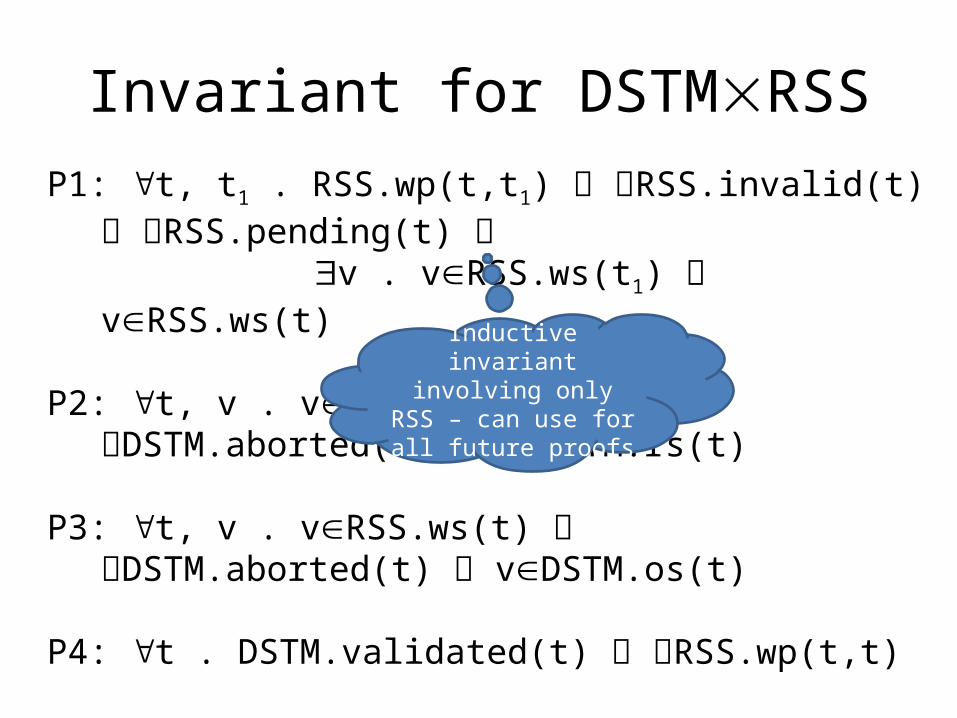
Invariant for DSTMRSSP1: t, t1 . RSS.wp(t,t1) RSS.invalid(t) RSS.pending(t)
v . vRSS.ws(t1) vRSS.ws(t)
P2: t, v . vRSS.rs(t) DSTM.aborted(t) vDSTM.rs(t)
P3: t, v . vRSS.ws(t) DSTM.aborted(t) vDSTM.os(t)
P4: t . DSTM.validated(t) RSS.wp(t,t)
P5: t . DSTM.validated(t) RSS.invalid(t)
P6: t . DSTM.validated(t) RSS.pending(t)
Inductive invariant involving only RSS – can use for all future proofs

Templates for DSTMRSSP1: t, t1 . 1(t,t1) 2(t) 3(t)
v . v4(t1) v5(t)
P2: t, v . v1(t) 2(t) v3(t)
P3: t, v . V1(t) 2(t) v3(t)
P4: t . 1(t) 2(t,t)
P5: t . 1(t) 2(t)
P6: t . 1(t) 2(t)

Templates for DSTMRSSt, t1 . 1(t,t1) 2(t) 3(t) v . v4(t1) v5(t)
t, v . v1(t) 2(t) v3(t)
t . 1(t) 2(t,t)
Why templates?• Makes invariant separable• Controls complexity of invariants• Adding templates enables refinement

Mining candidate invariants
• Use predefined set of templates to specify structure of candidate invariants– t,v . 1 2 3
– 1, 2, 3 are predicates of M or their negations
– Existential formulas capturing 1-level conflictsv . v4(t1) v5(t2)
• Mine candidate invariants from concrete execution
85

Iterative invariant weakening
• Initial candidate invariant C0=P1 P2 … Pk• Try to prove I2: transition ’
C1 = { Pi | I0 transition Pi for PiI0}
• If C1=C0 then we have an inductive invariant• Otherwise, compute
C2 = { Pi | C1 transition Pi for PiC1}• Repeat until either– found inductive invariant – check I3: Ck SIM– Reached top {} – trivial inductive invariant
I1: Initial I2: transition ’ I3: SIM
DSTM RSS SIM
86

Weakening illustration
P1 P2 P3 P1 P2 P3

Abstract proof rule
I1: (Initial) I2: abs_transition(()) ’ I3: () SIM
DSTM RSS SIM
I1: Initial I2: transition ’ I3: SIM
DSTM RSS SIM
Formulaabstraction
Abstracttransformer
Approximateentailment
88

Conclusion
• Novel invariant generation using templates – extends applicability of invisible invariants
• Abstract domain and reasoning to check invariants without state explosion
• Proved strict-serializability for TPL, DSTM, TL2– BLAST and TVLA failed
89

Verification resultsproperty TPL DSTM TL2 RSS
Bound for invariant gen.
(2,1) (2,1) (2,1) (2,1)
No. cubes 8 184 344 7296
Bounded time 4 8 10 23
Invariant mining time
6 13 26 57
#templates 28 28 28 28
#candidates 22 53 97 19
#proved 22 30 68 14
#minimal 4 8 5 -
avg, time per invariant
3.7 20.3 36 43.4
avg. abs. size 31.7 256.9 1.19k 2.86k
Total time 3.5m 54.3m 129.3m 30.9m
90

Insights on transactional memories
• Transition relation is symmetric – thread identifiers not usedp’(t,v) … t1 … t2
• Executing thread t interacts only with arbitrary thread or conflict-adjacent thread
• Arbitrary thread:v . vTL2.rs(t1) vTL2.ws(t1)
• Conflict adjacent:v . vDSTM.rs(t1) vDSTM.ws(t)
91

v1
readset
writeset
v2
t2
t
t3
writeset
read-writeconflict
write-writeconflict
Conflict adjacency
92
v . vrs(t) vDSTM.ws(t2)v . vws(t1) vDSTM.ws(t2)

......
t2
t
t3
Conflict adjacency
93

Related work
• Reduction theoremsGuerarroui et al. [PLDI’08,CONCUR’08]
• Manually-supplied invariants – fixed number of threads and variables + PVSCohen et al. [FMCAS’07]
• Predicate Abstraction + Shape Analysis– SLAM, BLAST, TVLA
94

Related work
• Invisible invariantsArons et al. [CAV’01] Pnueli et al. [TACAS’01]
• Templates – for arithmetic constraints• Indexed predicate abstraction
Shuvendu et al. [TOCL’07]• Thread quantification
Berdine et al. [CAV’08]Segalov et al. [APLAS’09]
95

96
Thank You!
Recommended