5/13/2018 Prof.johnson July16 APSS2010 - slidepdf.com
http://slidepdf.com/reader/full/profjohnson-july16-apss2010 1/9

5/13/2018 Prof.johnson July16 APSS2010 - slidepdf.com
http://slidepdf.com/reader/full/profjohnson-july16-apss2010 2/9

5/13/2018 Prof.johnson July16 APSS2010 - slidepdf.com
http://slidepdf.com/reader/full/profjohnson-july16-apss2010 3/9
USC ViterbiSchool of Engineering
Example 2DOF System
Unforced Case — free responses
Review SDOF: modal free responses of is
where the ai & bi , or c i & " i , depend on and
k 1!=!4
k 2!=!2
2
1
˙q i +" i
2q i = 0
q i (t ) =a i sin" i t +b i cos" i t = c i sin(" i t +# i )
q i (0) !!!!!!! q i (0)
For example, with initial conditions:
q 1 (0) =1= a
1sin0+ b
1cos0 =c
1sin("
1)
q 1 (0) = 0 =a 1# 1cos0 $b 1# 1sin0 = c 1# 1cos(" 1)
q 2(0) = 0 = a 2 sin0+ b 2 cos0 = c 2 sin(" 2)
q 2(0) =1=a 2#
2cos0 $b 2#
2sin0 = c 2#
2cos("
2)
then: a1=0, b1=1, c 1=1, " 1=–! /2 and a 2=1/2, b 2=0, c 2=1/2, " 2=0.
q 1 (t ) = cost
q 2(t ) = 0.5sin2t
More generally, the responses in the original coordinates are:
u(t ) = "i a i sin#
i t +b
i cos#
i t [ ]
i
$ = c i "i sin(#
i t +%
i )
i
$
= ai sin"
i t +bi cos"
i t [ ]i
# = ci sin("
i t +$ i )
i
#
USC ViterbiSchool of Engineering
Example 2DOF System
Example Free Responses
Displaced in shape of: 2nd mode1st mode combination
USC ViterbiSchool of Engineering
c 2!=!0.1
Example 2DOF System
Unforced Case with Damping
Let’s add damping. (What is damping???)
k 1!=!4
k 2!=!2
2
1
k 1!=!4 k 2!=!1m 1!=
!2 m 2
!=
!1
c 1!=!0.2
c 2!=!0.1
c 1!=!0.2
Already know " =
1 1
2 #1
$
% &
'
( ) . Let u ="q and premultiply by " T
M ˙u+Cu+Ku =0
C =
c 1+c
2"c
2
"c 2
c 2
#
$ %
&
' ( =
0.3 "0.1
"0.1 0.1
#
$ %
&
' (
1 2
1 "1
#
$ %
&
' (
2 0
0 1
#
$ %
&
' (
1 1
2 "1
#
$ %
&
' (
˙q 1
˙q 2
) * +
, - . +
1 2
1 "1
#
$ %
&
' (
0.3 "0.1
"0.1 0.1
#
$ %
&
' (
1 1
2 "1
#
$ %
&
' ( q
1
q 2
) * +
, - . +
1 2
1 "1
#
$ %
&
' (
6 "2
"2 2
#
$ %
&
' (
1 1
2 "1
#
$ %
&
' ( q
1
q 2
) * +
, - .
=
6 0
0 3
#
$ %
&
' (
˙q 1
˙q 2
) * +
, - . +
0.3 0
0 0.6
#
$ %
&
' ( q
1
q 2
) * +
, - . +
6 0
0 12
#
$ %
&
' ( q
1
q 2
) * +
, - . =
0
0
) * +
, - .
"TM" ˙q+"TC"q+"TK"q =0
"
˙q 1 +
0.05q 1 +
1q 1 = 0
˙q 2+0.20q
2+ 4q
2= 0
˙q i +2" i # i
˙q i +# i q i = 0
" 1
= 1, # 1=0.025 =2.5%
" 2 =
2, # 2 =
0.050 =5.0%
USC ViterbiSchool of Engineering
c 2!=!0.1
Example 2DOF System
Unforced Case with Damping — free response
So modal damped free responses are
where the ai & bi , or c i & " i , depend on and , and.
k 1!=!4
k 2!=!2
2
1
k 1!=!4 k 2!=!1m 1!=
!2 m 2
!=
!1
c 1!=!0.2
c 2!=!0.1
c 1!=!0.2
q i (t ) =a i e "# i $ i t sin$ i
dt +b i e "# i $ i t cos$ i
dt = c i e "# i $ i t sin($ i
dt +% i )
q i (0) !!!!!!! q i (0)
More generally, the responses in the original coordinates are:
u(t ) = e "# i $ i t %
i a i sin$
i
dt +b
i cos$
i
dt [ ]
i
& = c i %i e "# i $ i t sin($
i
dt +
i
&
= e "# i $ i t a
i sin$
i
dt +b
i cos$
i
dt [ ]
i
& = ci e "# i $ i t sin($
i
dt +'
i
i
&
" i d=" i [1#$ i
2]1/2
USC ViterbiSchool of Engineering
General MDOF Systems
Equation of motion: M˙
u+C˙
u+Ku =Ef
First use the undamped, unforced equation to find natural
frequencies and mode shapes:(M"
2#K)$ =0 or ("
2I#M
#1K)$ =0
The mode shapes have the properties that
"i TM" j =M i # ij =
M i , i = j
0, i $ j
% & '
"i TK" j =K i # ij =
K i , i = j
0, i $ j
% & '
The fact that !i TM! j = 0 and !i
TK! j = 0 for i ! j means the
mode shapes are orthogonal . Note also that K i /M i = ! i 2.
Note: some systems have (M! 2 – K) be less than rank (n – 1), whichimplies there are multiple modes at one or more frequencies.
Note: some systems (e.g., satellites) may have ! = 0 be a solution;
this implies one or more rigid body modes in which the wholestructure moves or rotates, possibly without internal deformation.
USC ViterbiSchool of Engineering
General MDOF Systems
Forced Harmonic Response
Forced response of a linear system is the sum of the freeresponse from any non-zero initial conditions and theeffects of the external forcing.
Let us assume the initial conditions are zero and consider a harmonic excitation.
M ˙u +Cu+Ku =Ef =Ef0sin" t
Then the response is also harmonic. This is most easily
demonstrated using a SDOF example …
5/13/2018 Prof.johnson July16 APSS2010 - slidepdf.com
http://slidepdf.com/reader/full/profjohnson-july16-apss2010 4/9
5/13/2018 Prof.johnson July16 APSS2010 - slidepdf.com
http://slidepdf.com/reader/full/profjohnson-july16-apss2010 5/9
USC ViterbiSchool of Engineering
Damping Models
In the previous damped 2DOF example, we used specific
damping coefficients in the model: c 1 = 0.2, c 2 = 0.1.
k 1!=!4
k 2!=!2
2
1c 2!=!0.1
c 1!=!0.2
2 0
0 1
"
# $
%
& '
˙u 1
˙u 2
( ) *
+ , - +
0.3 .0.1
.0.1 0.1
"
# $
%
& ' u 1
u 2
( ) *
+ , - +
4 +2 .2
.2 2
"
# $
%
& ' u 1
u 2
( ) *
+ , - =
0
0
( ) *
+ , -
" TC" =
1 2
1 #1
$
% &
'
( )
0.4 #0.2
#0.2 0.2
$
% &
'
( ) 1 1
2 #1
$
% &
'
( ) =
0.4 #0.2
#0.2 1
$
% &
'
( )
"
˙q 1 +
1
15q 1 #
1
30q 2 +
1q 1
= 0
˙q 2+
1
3q 2#
1
15q 1+ 4q
2= 0
" 1
= 1, # 1=2.5%
" 2=2, #
2=5.0%
We found that the damping #TC# diagonalized.
However, a different choice (c 1 = 0.2, c 2 = 0.2) may not:
0.2
c 2!=!0.1
k 1!=!4 k 2!=!1m 1!=!2 m 2!=!1
c 1!=!0.2 0.2
This is what is called a non-proportionally
damped or non-classically damped system.
The equations
are still coupled!
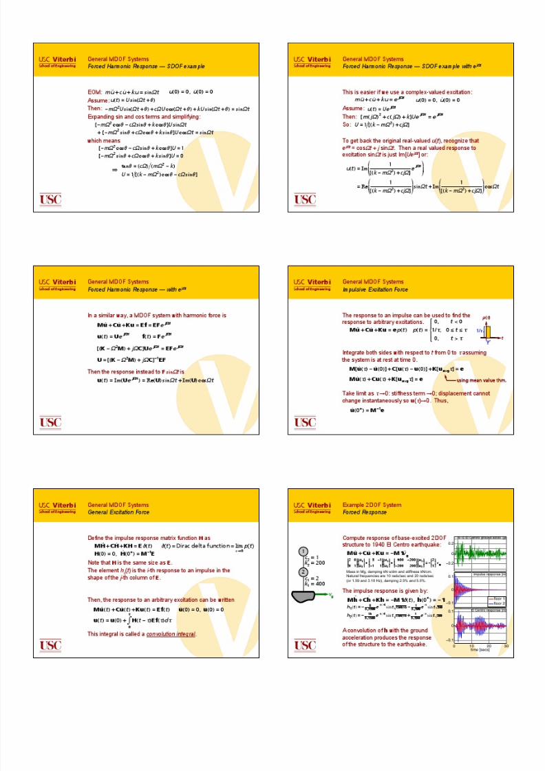
We will see later how to solve systems like this.(! 1=1.00037, ! 2=1.99926, & 1=3.3313%, & 2=8.3368%)
USC ViterbiSchool of Engineering
Damping Models
Special Cases of Proportional Damping: Modal Damping
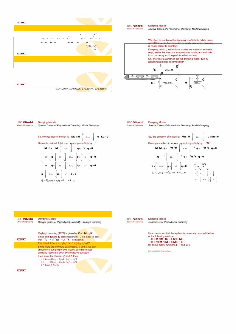
We often do not know the damping coefficients (while mass
and stiffness can be computed or easily measured, dampingis much harder to quantify).
Damping ratios & i in individual modes are easier to estimate(e.g., excite the structure in a particular mode, and estimate & from the decay e –&! t ; repeat for other modes).
So, one way to construct the full damping matrix C is byassuming a modal decomposition
" TC" =
! 02# i $ i M i
0 !
%
&
' ' '
(
)
* * *
C =" # T! 0
2$ i % i M i
0 !
&
'
( ( (
)
*
+ + + " #1 =M"
! 02$ i % i
0 !
&
'
( ( (
)
*
+ + + " #1
USC ViterbiSchool of Engineering
Damping Models
Special Cases of Proportional Damping: Modal Damping
So, the equation of motion is: M ˙u+M"!
2# i $ i
!
%
& ' '
(
) * * " +1u+Ku =0
Decouple method 1: let u = #q and premultiply by #T:
" TM" ˙q+" TM"!
2# i $ i
!
%
& ' '
(
) * * " +1"q+" TK"q =0
!
M i
!
%
& ' '
(
) * * ˙q+
!
M i
!
%
& ' '
(
) * *
!
2# i $ i
!
%
& ' '
(
) * * q+
!
K i
!
%
& ' '
(
) * * q =0
!
M i
!
%
& ' '
(
) * * ˙q+
!
M i
!
%
& ' '
(
) * *
!
2# i $ i
!
%
& ' '
(
) * * q+
!
K i
!
%
& ' '
(
) * * q =0
˙q+
!
2# i $ i
!
%
& '
'
(
) *
* ˙q+
!
$ i
2
!
%
& '
'
(
) *
* q=
0
˙q i +2# i $ i q i +$ i 2q i =0, i =1,...,n
USC ViterbiSchool of Engineering
Damping Models
Special Cases of Proportional Damping: Modal Damping
So, the equation of motion is: M ˙u+M"!
2# i $ i
!
%
& ' '
(
) * * " +1u+Ku
Decouple method 2: let u = #q and premultiply by # –1M –1:
" #1M#1M" ˙q+" #1M#1M"!
2$ i % i
!
&
' ( (
)
* + + " #1"q+" #1M#1K"q =
" #1" ˙q+" #1"!
2$ i % i
!
&
' ( (
)
* + + " #1"q+" #1M#1K"q =0
Let " =#$1M
$1K#
% M#" =K# % #T
M#" =#TK#
% ! M i
!
&
' (
(
)
* +
+ " =
!
K i
!
&
' (
(
)
* +
+
% " =
!
K i M i
!
&
' ( (
)
* + + =
!
, i 2
&
' ( (
˙q+
!
2" i # i
!
$
% & &
'
( ) ) q+
!
# i 2
!
$
% & &
'
( ) ) q =0
˙q i +2" i # i q i +# i 2q i = 0, i =1,...,n
USC ViterbiSchool of Engineering
Damping Models
Special Cases of Proportional Damping: Rayleigh Damping
Rayleigh damping (1877) is given by C = ' M + ( K.Since both M and K diagonalize with #, it is easy to see
that #TC# = ' #TM# + ( #TK# is diagonal.
The result: 2& i ! i = ' + (! i 2 or & i = (' /! i + (! i )/2.
Since there are only two parameters, ' and ( , we can
choose the damping of two modes; all other modal
damping ratios are given by the above equation.
If we know (or choose) & r and & s then' = 2! r ! s(& r ! s – & s! r ) / (! s
2 – ! r 2)
( = 2(& s! s – & r ! r ) / (! s2 – ! r
2)& i = (' /! i + (! i )/2
USC ViterbiSchool of Engineering
Damping Models
Conditions for Proportional Damping
It can be shown that the system is classically damped if either of the following are true:• C = M F(M –1K) + K G(K –1M)
• C = F(KM –1)!M + G(MK –1) K for some matrix functions F(") and G(").
Note: should add references here.

5/13/2018 Prof.johnson July16 APSS2010 - slidepdf.com
http://slidepdf.com/reader/full/profjohnson-july16-apss2010 6/9
USC ViterbiSchool of Engineering
Laplace and Fourier Transforms
Time history p(t ) is related to its
Laplace transform P (s) and Fourier Transform P ( j ! ) as
P (s ) = p (t )e "st dt "#
#
$
p (t ) =1
2"
P (s )e st ds
#$
$
%
P ( j " ) = p (t )e # j " t dt
#$
$
%
p (t ) =1
2" P ( j # )e j # t d #
$%
%
&
Laplace transform P (s) may also be denoted L{ p(t )}
and Fourier Transform P ( j ! ) by F { p(t )}.
Note: L p (t ){ } = p (t )e "st dt "#
#
$ = pe "st "#
#+ p (t )se "st dt
"#
#
$ = s L p (t ){ }
(assuming p(t )$0 as t $#)integration by parts
Similarly: F p (t ){ } = j " F p (t ){ }
USC ViterbiSchool of Engineering
Transfer Functions
SDOF
Consider single degree of freedom system m u +c u +ku =f
ms 2U (s )+csU (s )+kU (s ) =F (s )
(ms 2+cs +k )U (s ) =F (s )
U (s )
F (s )=
1
ms 2+cs +k
Laplace transform both sides:
Or, rearranging:
U ( j " )
F ( j " )=
1
m ( j " )2+cj "
=
1
k #m " 2+cj
Could do similar using Fourier transform:
If f (t ) = F 0 sin! t , then
u (t ) = F 0
1
k "m # 2+cj #
sin(# t +$ )
" = angle1
k #m $ 2+cj $
%
& '
(
) * = tan
#1 c
m $ 2 #k
These are calledtransfer function
USC ViterbiSchool of Engineering
Transfer Functions
SDOF Example
For example:
k !=!8
2c !=!0.2
2˙u +0.2u +8u =f
10−1
100
101
10−2
10−1
100
Frequency [rads/sec]
M a g n i t u d e
10−1
100
101
−150
−100
−50
0
Frequency [rads/sec]
P h a s e [ d
e g r e e s ]
10−1
100
101
−2
0
2
Frequency [rads/sec]
R e a l P a r t
10−1
100
101
−3
−2
−1
0
Frequency [rads/sec]
I m a g i n a r y P a r t
U (s )
F (s )=
1/2
s 2+0.1s + 4 Graph with s = j ! :
USC ViterbiSchool of Engineering
Transfer Functions
SDOF Example — Poles
For example:
k !=!8
2c !=!0.2
2˙u +0.2u +8u =f
U (s )
F (s )=
1/2
s 2+0.1s + 4
Roots of the denominator polynomial are called the poles
of the system:
s poles ="0.1± 0.12 " 4
2= "0.05 ± j 3.9975 # "0.05 ±1.9994
R
Im
USC ViterbiSchool of Engineering
Transfer Functions
SDOF Example — Poles and Zeros
Some TFs have a numerator that is also a polynomial in s.For example, the transfer function from ground accelerationto the absolute acceleration of a SDOF system:
k !=!8
2c !=!0.2
2˙u +0.2u +8u = "2˙v g
L ˙v (t ){ }
L ˙v g(t ){ }=
L ˙u + ˙v g{ }L ˙v g(t ){ }
=
L "0.1u " 4u { }
L ˙v g(t ){ }
= ("0.1s " 4)L u { }
L ˙v g(t ){ }=
0.1s + 4
s 2+0.1s + 4
Roots of the numerator polynomial are
called the zeros of the system:
s root =
"40
Re
Im
USC ViterbiSchool of Engineering
Transfer Functions
MDOF
For a MDOF system, must be careful to handle matricescorrectly in determining the transfer function:
M ˙u+Cu+Ku =Ef
Ms 2+Cs +K[ ]U(s ) =EF(s )
U(s ) = Ms 2+Cs +K[ ]
"1
EF(s )
Now, the transfer function [Ms2 + Cs + K] –1E is a matrix,
each element of which is a scalar transfer function.

5/13/2018 Prof.johnson July16 APSS2010 - slidepdf.com
http://slidepdf.com/reader/full/profjohnson-july16-apss2010 7/9

5/13/2018 Prof.johnson July16 APSS2010 - slidepdf.com
http://slidepdf.com/reader/full/profjohnson-july16-apss2010 8/9
USC ViterbiSchool of Engineering
State-Space Formulation
Unforced Response — Mode Shapes
If the damping term does not decouple, then the state-
space approach must be used and
must be solved directly to get the complex eigenvalues and
complex eigenvectors. Once the the eigenvalues ) i ,) i * are
found, then ! i = |) i | and & i = –Re{) i }/(2! i ).
If some eigenvalues are purely real, then no oscillator
mode corresponds to that eigenvalue.
(" 2I+ " M
#1C +M
#1K)$
d=0
USC ViterbiSchool of Engineering
k 3!=!a
1c 3!=!c
k 2!=!a
1c 2!=!c
State-Space Formulation
Visualization of Non-Proportional Damping
Let’s look at an example of a
3DOF structure with classicaldamping (-c = 0). The natural
frequencies & damping are:! 1 = 1 , & 1 = 3.14%;! 2 = 2.80, & 2 = 8.80%;
! 3 = 4.05, & 3 = 12.72%.
A non-classically dampedversion with additional
damping in the first floor (-c = 15c ) has natural
frequencies & damping:! 1 = 1.15, & 1 = 23.6%;! 2 = 2.71, & 2 = 85.9%;
! 3 = 3.64, & 3 = 15.7%.
k 1!=!a
1
c 1!=!c !+!-c
c !=!0.01a
a !=!199.3233(so first natural
frequency is 1!Hz)
"0.328 0.737 "0.591
"0.591 0.328 0.737
"0.737 "0.591 "0.328
0.065± 2.06 j "1.142!12.9 j 1.913±1
0.117± 3.71 j "0.508! 5.8 j "2.385!1
0.146± 4.63 j 0.916±10.4 j 1.061±
#
$
% % % % % % %
"0.233! 0.19 j "0.545! 3.99 j 0.003± 0
"0.557! 0.08 j "0.977! 0.93 j 0.537! 0
"0.737 "0.591 "0.328
"0.966±1.97 j "26.85± 63.2 j 3.749! 0
0.409± 4.04 j 6.213± 22.1 j "3.575!1
1.260± 5.17 j 8.655± 5.2 j 1.174± 7
#
$
% % % % % % %
USC ViterbiSchool of Engineering
State-Space Formulation
Visualization of Non-Proportional Damping
ProportionallyDamped:
Non-Proportionally
Damped:
USC ViterbiSchool of Engineering
State-Space Formulation
Unforced Free Response
The unforced free response of the state-space system
could be found through modal decomposition, but there is aneasier way. To compute the response at time t , break the time
up into r smaller steps. Given the definition of a derivative:
˙" =A"
"(1
r t ) # "(0
r t )+ " 1
r t # "(0)+A"(0) 1
r t = [I+A t
r ]"(0)
The same can be used to approximate ( after each t /r .
"(2r t ) # [I+A t
r ]"(1
r $t ) = [I+A t
r ]2"(0)
!
"(r
r t ) # [I+A t
r ]"(r %1
r $t ) = [I+A t
r ]r "(0)
To eliminate the approximation, let r $#.
"(t ) = [I+ (At ) + 1
2!(At )
2+
1
3!(At )
3+!]"(0)
"(t ) =e At "(0)
USC ViterbiSchool of Engineering
State-Space Formulation
Unforced Free Response — Notes about eAt
eAt is a matrix; its elements are not the exponential of theelements of At . The computation of eAt can be computedthrough the power series formulation, though that is not
computationally efficient.
An efficient computation uses the fact that the eigenvectors of
a power of a matrix are the same as those of the matrix itself.
If A+ = +., where + is the eigenmatrix and . is a diagonalmatrix of eigenvalues, then it can be shown that An+ = +.n.
Thus, e At
= I+ (At ) + 1
2!(At )
2+
1
3!(At )
3+!
="#1" +"#1$"t +1
2!"#1$"2
t 2+
1
3!"#1$3"t
3+!
="#1[I+ ($t ) + 1
2!($t )
2+
1
3!($t )
3+!]"
= "#1
"
e % i t
"
&
'
( ( (
)
*
+ + +
"
USC ViterbiSchool of Engineering
State-Space Formulation
Impulse Response
The state impulse response matrix is given by
H" =AH" +B# (t ), H" (0$) = 0
Hy =CyH" +Dy# (t )
Integrating from t = 0 – to t = 0+, will give the initial conditions
that make a free response equal to the impulse response.
H"(0
+
) #H"(0#) =AH"
avg(0
+
#0#)+B
0 0
H" (0+
) =B
For t > 0, the impulse response is just an unforced free
response (which was solved several slides ago), so
H"(t ) =e
At H
"(0
+
)
H" (t ) =e At B
5/13/2018 Prof.johnson July16 APSS2010 - slidepdf.com
http://slidepdf.com/reader/full/profjohnson-july16-apss2010 9/9
USC ViterbiSchool of Engineering
State-Space Formulation
Forced Response
The forced response is, then, the combination of the initial
condition free response and the effects of the force
"(t ) =e At "(0)+ e
A(t #$ )Bf($ )d $
0
t
%
Add Example!USC ViterbiSchool of Engineering
Discrete-Time State-Space System
We’ve already seen the free response of the unforced state-
space system . So, ((t + -t ) = eA-t ((t ).
The effect of the forced response of in [t , t + -t ]
is the superposition of the free response with the impulse
response of f during the time step.
˙" =A"
Defining ((k ) = ((k -t ), then the discrete-time state space form
"(k +1) = Ad"(k )+B
df(k )
y(k ) =Cy"(k )+Dyf(k )
˙" =A" +Bf
"(t +
#t )=e
A#t
"(t )+ e
A(t +#t $% )
t
t +#t
& Bf
(%
)d %
In the interval [t , t + -t ), if f($ ) is constant (a zero-order hold )
"(t +#t ) =e A#t
"(t ) + e A(#t $% )
0
#t
& d %
'
( )
*
+ , Bf(t )
Ad
Bd
Ad Bd
0 I
"
# $
%
& ' =e
A
0
"
# $
Note: one can also assume a first-o
(linear) hold on f to determine Bd.
USC ViterbiSchool of Engineering
Distributed Parameter Systems
Euler-Bernoulli Beam Example
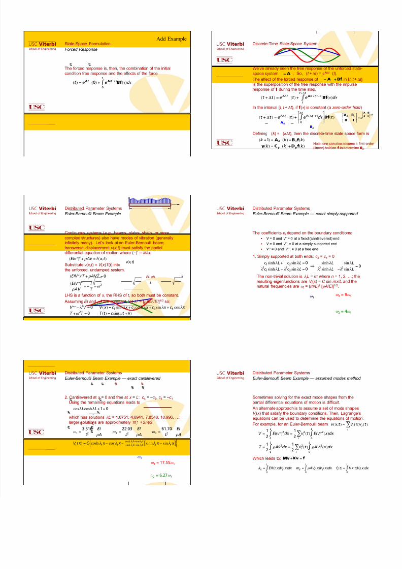
Continuous systems (e.g., beams, plates, shells, or more
complex structures) also have modes of vibration (generallyinfinitely many). Let’s look at an Euler-Bernoulli beam;
transverse displacement v ( x ,t ) must satisfy the partialdifferential equation of motion where (")/ = 0/0 x :
(EI " " v " " ) + # A ˙v =f (x ,t )
L
x
v (x ,t )
EI , * A
Substitute v ( x ,t ) = V ( x )T (t ) into
the unforced, undamped system.
(EI " " V " " ) T + # AV T = 0
(EI " " V " " )
# AV = $
˙T
T
LHS is a function of x , the RHS of t , so both must be constant.
=" 2
˙T +"
2T = 0
" " " " V # $ 4V =0
Assuming EI and * A are constant, let ) 4 = [* A! 2/EI ]1/2 so:
V (x ) =c 1sinh" x +c
2cosh" x +c
3sin" x +c
4cos" x
T (t ) = c sin(" t +# )
USC ViterbiSchool of Engineering
Distributed Parameter Systems
Euler-Bernoulli Beam Example — exact simply-supported
The coefficients c i depend on the boundary conditions:
• V = 0 and V / = 0 at a fixed (cantilevered) end
• V = 0 and V // = 0 at a simply supported end
• V // = 0 and V /// = 0 at a free end
1. Simply supported at both ends: c 2 = c 4 = 0
c 1sinh" L + c
3sin" L = 0
" 2c 1sinh" L # "
2c 3 sin" L = 0
$ sinh" L sin" L
" 2sinh" L #"
2sin" L
= 0
The non-trivial solution is ) i L = i ! where n = 1, 2, …; the
resulting eigenfunctions are V i ( x ) = C sin i ! x /L and thenatural frequencies are ! i = (i ! /L)2 [* A/EI ]1/2.
! 3!=!9! 1
! 2!=!4! 1! 1
USC ViterbiSchool of Engineering
Distributed Parameter Systems
Euler-Bernoulli Beam Example — exact cantilevered
cos" L cosh" L +1= 0
which has solutions ) L = 1.8751, 4.6941, 7.8548, 10.996, …;
larger solutions are approximately ! (1"+ 2n)/2.
! 3!=!17.55! 1
! 2!=!6.27! 1
! 1
2. Cantilevered at x = 0 and free at x = L: c 4 = –c 2, c 3 = –c 1 Using the remaining equations leads to
" 1=
3.516
L2
EI
# A
" 2=
22.03
L2
EI
# A
" 3=
61.70
L2
EI
# A
V i (x ) =C cosh"
i x # cos"
i x #
cosh" i L+cos" i L
sinh" i L+sin" i Lsinh"
i x # sin"
i x [ ]{ }
USC ViterbiSchool of Engineering
Distributed Parameter Systems
Euler-Bernoulli Beam Example — assumed modes method
Sometimes solving for the exact mode shapes from thepartial differential equations of motion is difficult.
An alternate approach is to assume a set of mode shapes
V i ( x ) that satisfy the boundary conditions. Then, Lagrange’s
equations can be used to determine the equations of motion.
For example, for an Euler-Bernoulli beam:
V =1
2EI ( " " v )2dx
0
L
# =
1
2v i
2(t ) EI " " V i
2(x )dx
0
L
# i
$
T =1
2% Av
2dx
0
L
# =
1
2v i
2(t ) % AV
i
2(x )dx
0
L
# i
$
f i (t ) = f (x ,t )V i (x )d0
L
"
v (x ,t ) = V i (x )v
i (t
i
"
Which leads to: M˙v +Kv = f
k ij = EI " " V i
(x ) " " V j (x )dx 0
L
#
m ij = " AV i (x )V j (x )dx 0
L
#
Recommended


![[ADVANCE - 13] INQ/PAGES/A SEC 10/30/11media.philly.com/documents/20111027_AFGHAN_13.pdf · July9 July18 July14 July15 July16 July17 July10 Seaman Aaron D. Ullom,](https://img.pdfslide.us/doc/110x75/5edda13fad6a402d6668c61e/advance-13-inqpagesa-sec-1030-july9-july18-july14-july15-july16-july17-july10.jpg)