M alkhozov,M ueller,Vedolin & Venter– 1
InternationalFunding Liquidity
Aytek M alkhozov
M cGill
Philippe M ueller
LSE
Andrea Vedolin
LSE
GyuriVenter
CBS
SQ A
23 July 2014

Introduction
Introduction
W hatwe do
W hatwe find
Illiquidity Proxies
M odel
Em piricalAnalysis
Conclusion
Appendix
M alkhozov,M ueller,Vedolin & Venter– 2
W hatwe do
M alkhozov,M ueller,Vedolin & Venter– 3
Providem easuresofcountry-leveland globalfunding illiquidity.
– 6 countries:Canada,Germ any,Japan,Switzerland,UK,US.
– M easuring noisein localyield curves,following Hu,Pan and W ang (2013).
Study thee ectthatthevariation in illiquidity overtim eand acrosscountrieshason internationalstock returns.
– Stylized internationalCAPM augm ented by m argin constraints,sim ilartoFrazziniand Pedersen (2013),to derivetestablepredictions.
– Study im pactofilliquidity on intercept/slopeofthesecurity m arketline.
– Exam ineperform anceofilliquidity/beta-sorted portfolios.
– M arket-neutraltrading strategies:Long levered high illiquidity-to-beta stocksand shortde-levered low illiquidity-to-beta stocks(BAIL).
W hatwe find
M alkhozov,M ueller,Vedolin & Venter– 4
Variation in liquidity m easurescan berelated to key m arketevents.
High correlation between localilliquidityindices,especiallyduring crisisperiods,butalso largeidiosyncraticfluctuations.
Globalilliquidity flattenstheSM L and increasesitsintercept.
Cross-country di erencein localilliquiditiesdrivesalphas.
Taking illiquidity into accountim provestheperform anceofthebetting-against-beta (BAB)strategy.

Illiquidity M easures
Introduction
Illiquidity Proxies
M otivation
Data
Term Structure
Sum m ary Stats
Correlations
Crisis
GlobalIlliquidity
M odel
Em piricalAnalysis
Conclusion
Appendix
M alkhozov,M ueller,Vedolin & Venter– 5
M otivation
M alkhozov,M ueller,Vedolin & Venter– 6
2 4 6 8 10
0.075
0.08
0.085
0.09
0.095Normal Day GE 22 July 91
maturity (in years)
yiel
d
0 2 4 6 8 10
0.075
0.08
0.085
0.09
0.095Black Wednesday GE 16 September 92
maturity (in years)
yiel
d
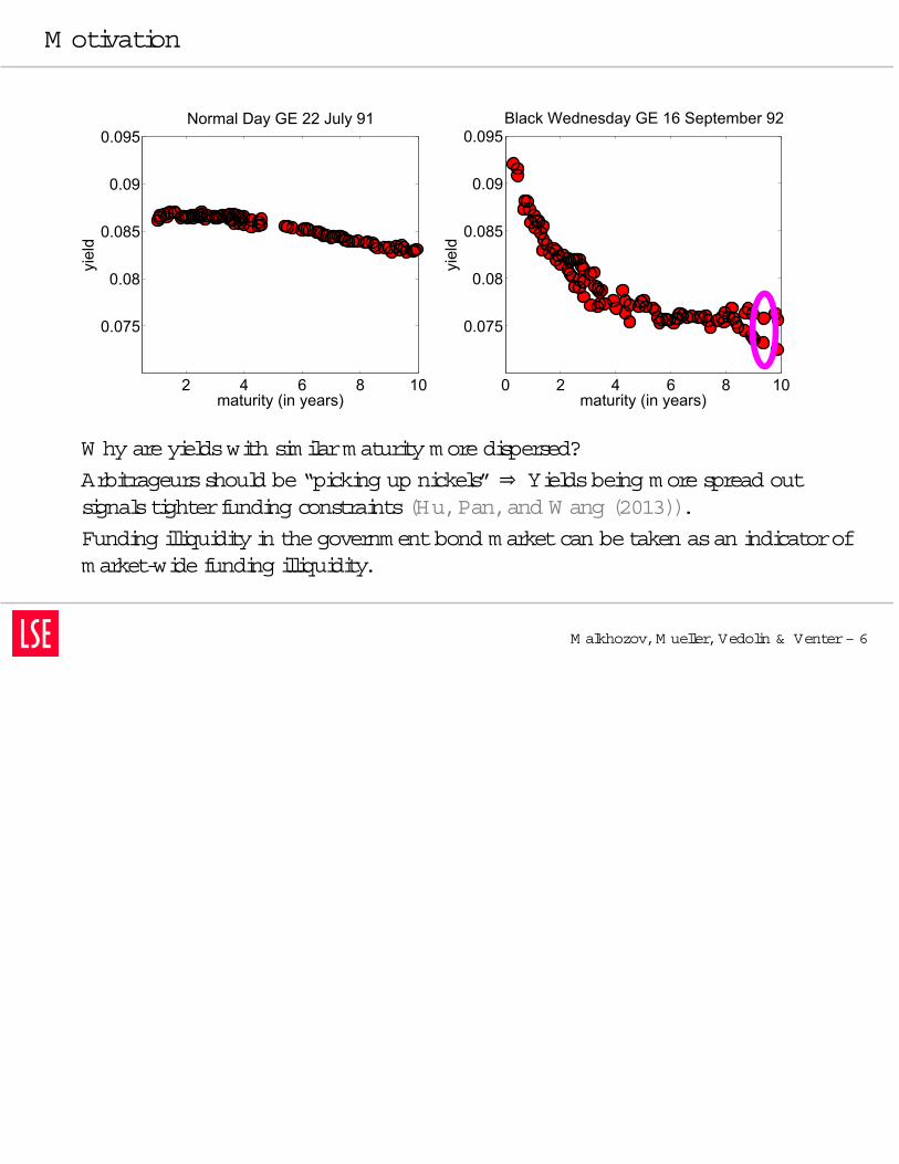
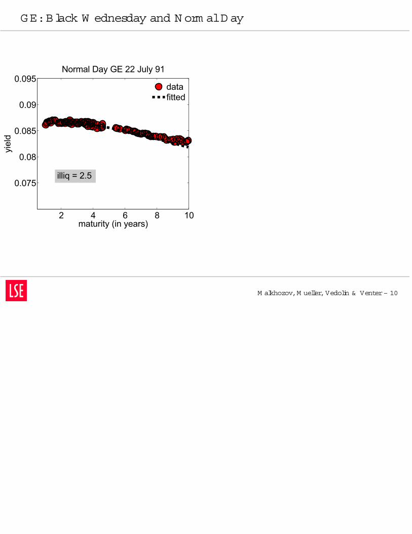
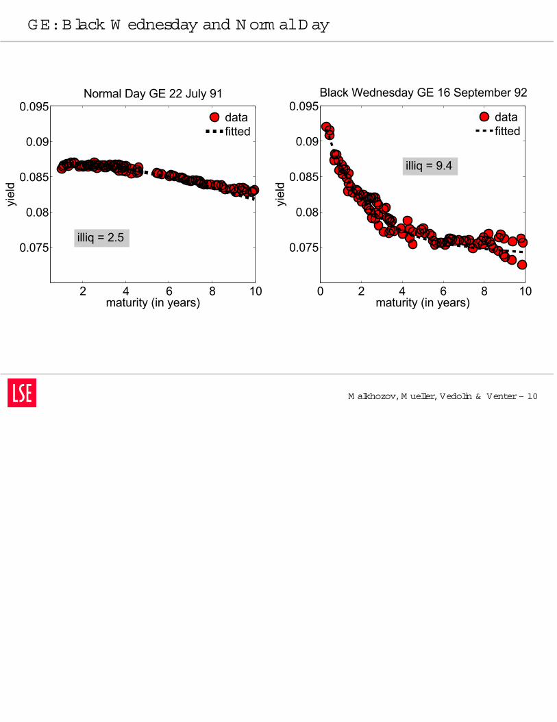
W hy areyieldswith sim ilarm aturity m oredispersed?
Arbitrageursshould be“picking up nickels”⇒ Yieldsbeing m orespread outsignalstighterfunding constraints(Hu,Pan,and W ang (2013)).
Funding illiquidityin thegovernm entbond m arketcan betaken asan indicatorofm arket-wide funding illiquidity.
D ata
Introduction
Illiquidity Proxies
M otivation
Data
Term Structure
Sum m ary Stats
Correlations
Crisis
GlobalIlliquidity
M odel
Em piricalAnalysis
Conclusion
Appendix
M alkhozov,M ueller,Vedolin & Venter– 7
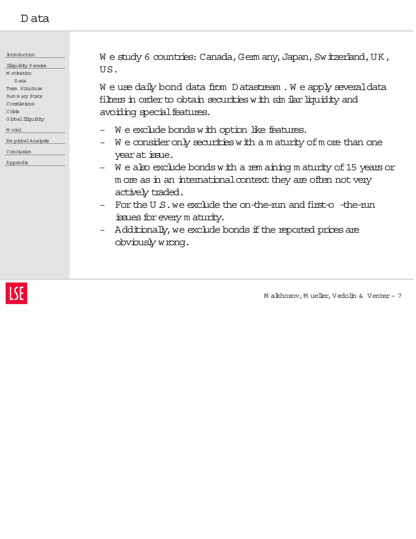
W e study 6 countries:Canada,Germ any,Japan,Switzerland,UK,US.
W e usedaily bond data from Datastream .W eapply severaldatafiltersin orderto obtain securitieswith sim ilarliquidityandavoiding specialfeatures.
– W e excludebondswith option likefeatures.– W e consideronly securitieswith a m aturity ofm orethan one
yearatissue.– W e also excludebondswith a rem aining m aturity of15 yearsor
m oreasin an internationalcontextthey areoften notveryactively traded.
– FortheU.S.we excludetheon-the-run and first-o -the-runissuesforevery m aturity.
– Additionally,we excludebondsifthereported pricesareobviously wrong.
InternationalTerm Structures
Introduction
Illiquidity Proxies
M otivation
Data
Term Structure
Sum m ary Stats
Correlations
Crisis
GlobalIlliquidity
M odel
Em piricalAnalysis
Conclusion
Appendix
M alkhozov,M ueller,Vedolin & Venter– 8
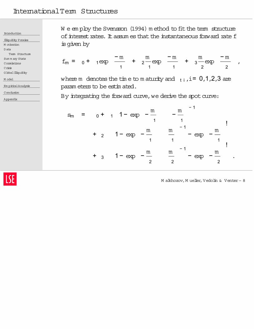
W e em ploy theSvensson (1994)m ethod to fittheterm structureofinterestrates.Itassum esthattheinstantaneousforward ratefisgiven by
fm = 0 + 1exp
− m
1
+ 2m
1exp
− m
1
+ 3m
2exp
− m
2
,
wherem denotesthetim eto m aturity and t i,i= 0,1,2,3 areparam etersto beestim ated.
By integrating theforward curve,we derivethespotcurve:
sm = 0 + 1
1− exp
−m
1
−m
1
− 1
+ 2
1− exp
−m
1
m
1
− 1
− exp
−m
1
!
+ 3
1− exp
−m
2
m
2
− 1
− exp
−m
2
!
.
Illiquidity Proxies
Introduction
Illiquidity Proxies
M otivation
Data
Term Structure
Sum m ary Stats
Correlations
Crisis
GlobalIlliquidity
M odel
Em piricalAnalysis
Conclusion
Appendix
M alkhozov,M ueller,Vedolin & Venter– 9
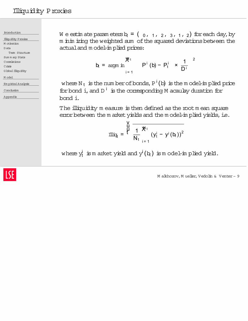
W eestim ateparam etersbt = ( 0, 1, 2, 3, 1, 2) foreach day,bym inim izing theweighted sum ofthesquared deviationsbetween theactualand m odel-im plied prices:
bt = argm inN tX
i = 1
P i (b) − P i
t
×
1D i
2
whereN t isthenum berofbonds,P i (b) isthem odel-im plied priceforbond i,and D i isthecorresponding M acaulay duration forbond i.
Theilliquidity m easure isthen defined astherootm ean squareerrorbetween them arketyieldsand them odel-im plied yields,i.e.
Illiqt =
vuut 1
Nt
N tX
i = 1
(yit − yi (bt ))
2
whereyit ism arketyield and y
i (bt ) ism odel-im plied yield.
GE:Black W ednesday and N orm alD ay
M alkhozov,M ueller,Vedolin & Venter– 10
2 4 6 8 10
0.075
0.08
0.085
0.09
0.095Normal Day GE 22 July 91
maturity (in years)
yiel
d
datafitted
illiq = 2.5
GE:Black W ednesday and N orm alD ay
M alkhozov,M ueller,Vedolin & Venter– 10
2 4 6 8 10
0.075
0.08
0.085
0.09
0.095Normal Day GE 22 July 91
maturity (in years)
yiel
d
datafitted
0 2 4 6 8 10
0.075
0.08
0.085
0.09
0.095Black Wednesday GE 16 September 92
maturity (in years)
yiel
d
datafitted
illiq = 2.5
illiq = 9.4
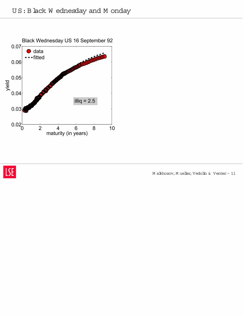
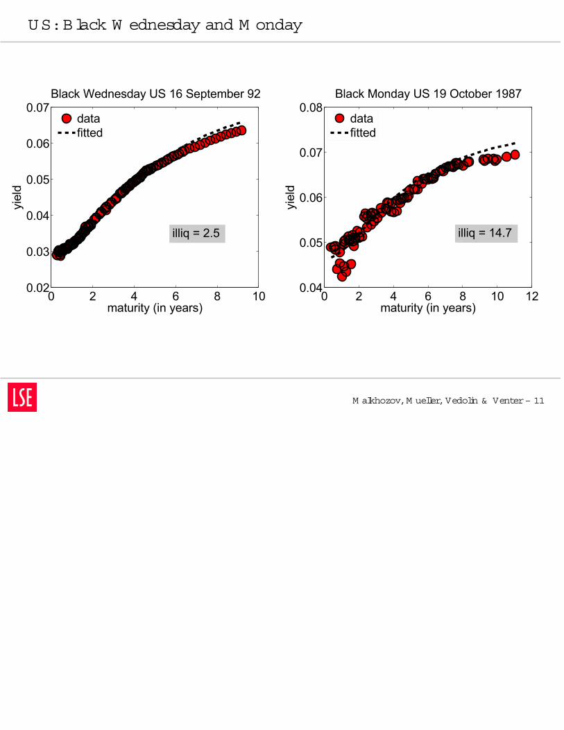
US:Black W ednesday and M onday
M alkhozov,M ueller,Vedolin & Venter– 11
0 2 4 6 8 100.02
0.03
0.04
0.05
0.06
0.07
maturity (in years)
yiel
d
Black Wednesday US 16 September 92
datafitted
illiq = 2.5
US:Black W ednesday and M onday
M alkhozov,M ueller,Vedolin & Venter– 11
0 2 4 6 8 100.02
0.03
0.04
0.05
0.06
0.07
maturity (in years)
yiel
d
Black Wednesday US 16 September 92
datafitted
0 2 4 6 8 10 120.04
0.05
0.06
0.07
0.08
maturity (in years)
yiel
d
Black Monday US 19 October 1987
datafitted
illiq = 2.5 illiq = 14.7
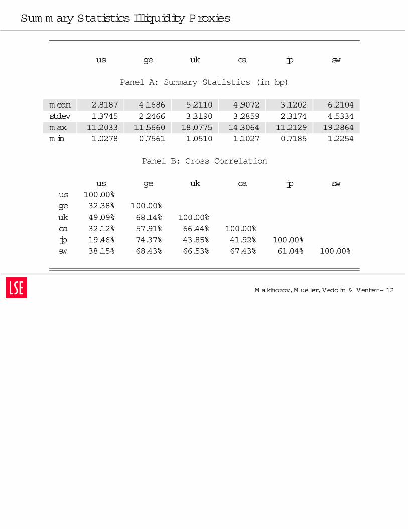
Sum m ary StatisticsIlliquidity Proxies
M alkhozov,M ueller,Vedolin & Venter– 12
us ge uk ca jp sw
Panel A: Summary Statistics (in bp)
m ean 2.8187 4.1686 5.2110 4.9072 3.1202 6.2104stdev 1.3745 2.2466 3.3190 3.2859 2.3174 4.5334m ax 11.2033 11.5660 18.0775 14.3064 11.2129 19.2864m in 1.0278 0.7561 1.0510 1.1027 0.7185 1.2254
Panel B: Cross Correlation
us ge uk ca jp swus 100.00%ge 32.38% 100.00%uk 49.09% 68.14% 100.00%ca 32.12% 57.91% 66.44% 100.00%jp 19.46% 74.37% 43.85% 41.92% 100.00%sw 38.15% 68.43% 66.53% 67.43% 61.04% 100.00%
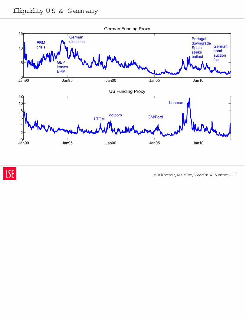
Illiquidity US & Germ any
M alkhozov,M ueller,Vedolin & Venter– 13
Jan90 Jan95 Jan00 Jan05 Jan100
5
10
15German Funding Proxy
Jan90 Jan95 Jan00 Jan05 Jan100
2
4
6
8
10
12US Funding Proxy
ERMcrisis
Germanelections
GBPleavesERM
Lehman
Germanbondauctionfails
PortugaldowngradeSpainseeksbailout
GM/ForddotcomLTCM
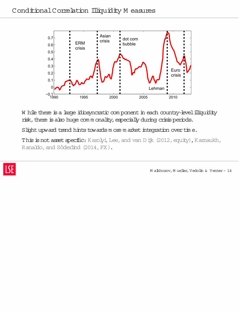
ConditionalCorrelation Illiquidity M easures
M alkhozov,M ueller,Vedolin & Venter– 14
1990 1995 2000 2005 2010−0.1
0
0.1
0.2
0.3
0.4
0.5
0.6
0.7
ERMcrisis
Asiancrisis dot com
bubble
Lehman
Eurocrisis
W hilethereisa largeidiosyncraticcom ponentin each country-levelilliquidityrisk,thereisalso hugecom m onality,especiallyduring crisisperiods.
Slightupward trend hintstowardsm orem arketintegration overtim e.
Thisisnotassetspecific:Karolyi,Lee,and van Dijk (2012,equity),Karnaukh,Ranaldo,and Soderlind (2014,FX).
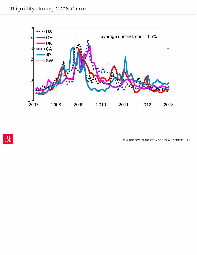
Illiquidity during 2008 Crisis
M alkhozov,M ueller,Vedolin & Venter– 15
2007 2008 2009 2010 2011 2012 2013−2
−1
0
1
2
3
4
5
USGEUKCAJPSW
average uncond. corr = 65%
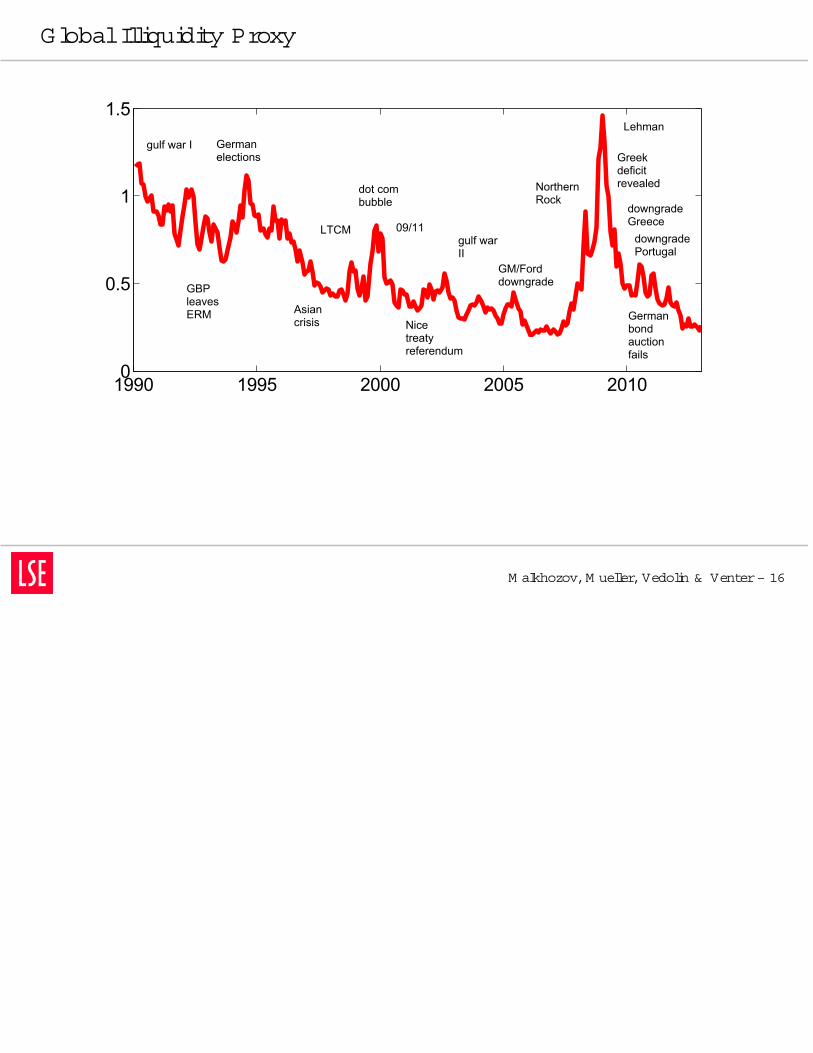
GlobalIlliquidity Proxy
M alkhozov,M ueller,Vedolin & Venter– 16
1990 1995 2000 2005 20100
0.5
1
1.5
Asian crisis
LTCM
dot combubble
09/11
Nicetreatyreferendum
gulf warII
GM/Forddowngrade
Lehman
Greekdeficit revealed
downgradeGreece
downgradePortugal
Germanbondauctionfails
GBPleavesERM
Germanelections
NorthernRock
gulf war I

M odel
Introduction
Illiquidity Proxies
M odel
M odel
CAPM
SM L
Sorted Portfolios
BAIL and BAB
Em piricalAnalysis
Conclusion
Appendix
M alkhozov,M ueller,Vedolin & Venter– 17

M odel
M alkhozov,M ueller,Vedolin & Venter– 18
Discrete-tim eOLG m odelwith 1 risklessand J risky assetsin supply jt .
Representativeagenthasm ean-variancepreferencesovernextperiod wealth
maxx t
xTt
Et [D t + 1 + Pt + 1] −
1 + rf
Pt
−
2xT
t Ωtxt
...and hasto postproportionalm argin ofm jt when investing x
jt P
jt in assetj:
s.t.X
j
m jt
xj
t
P j
t ≤ W t (1)
– m jt dependson agentand assetj,i.e.com binesboth investor-specificand
asset-specificcom ponents.
– Setting m arginsto zero m eansconstraint(1)neverbindsand thestandardCAPM holds.
W e assum ePPP holds,henceFX risk doesnotm atter.
Funding Liquidity CAPM
M alkhozov,M ueller,Vedolin & Venter– 19
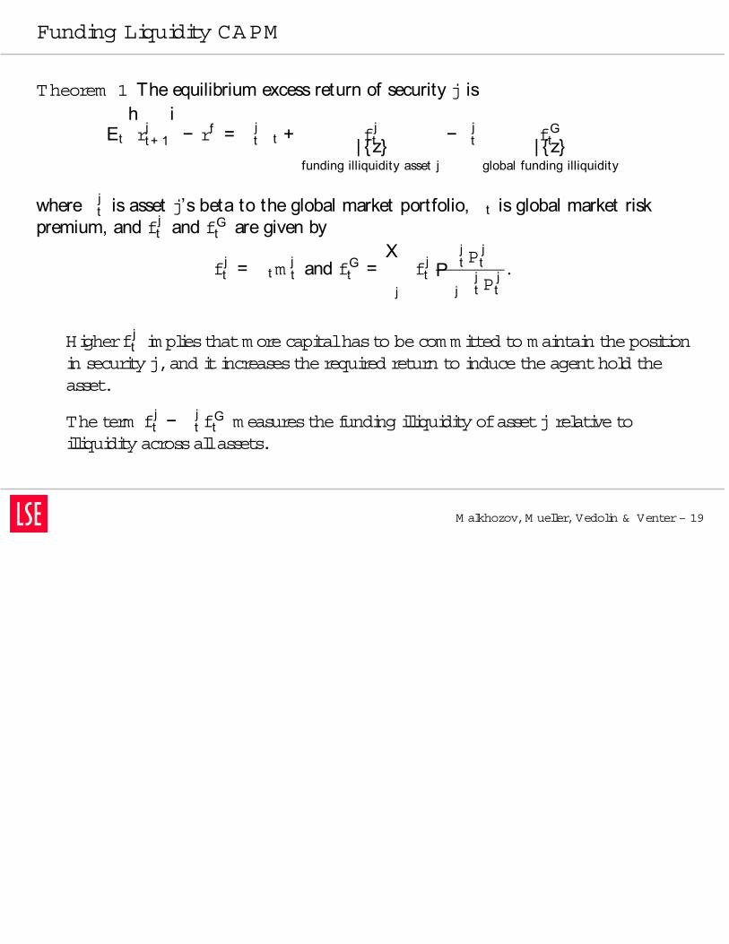
Theorem 1 The equilibrium excess return of security j is
Et
hrj
t + 1
i− rf = j
t t + fjt| z
funding illiquidity asset j
− jt fG
t| zglobal funding illiquidity
where jt is asset j’s beta to the global market portfolio, t is global market risk
premium, and fjt and fG
t are given by
fjt = tm
jt and fG
t =X
j
fjt
jt P
jtP
jjt P
jt
.
Higherfjt im pliesthatm orecapitalhasto becom m itted to m aintain theposition
in security j,and itincreasestherequired return to inducetheagenthold theasset.
Theterm fjt −
jt f
Gt m easuresthefunding illiquidity ofassetj relativeto
illiquidityacrossallassets.
Security M arketLine
Introduction
Illiquidity Proxies
M odel
M odel
CAPM
SM L
Sorted Portfolios
BAIL and BAB
Em piricalAnalysis
Conclusion
Appendix
M alkhozov,M ueller,Vedolin & Venter– 20
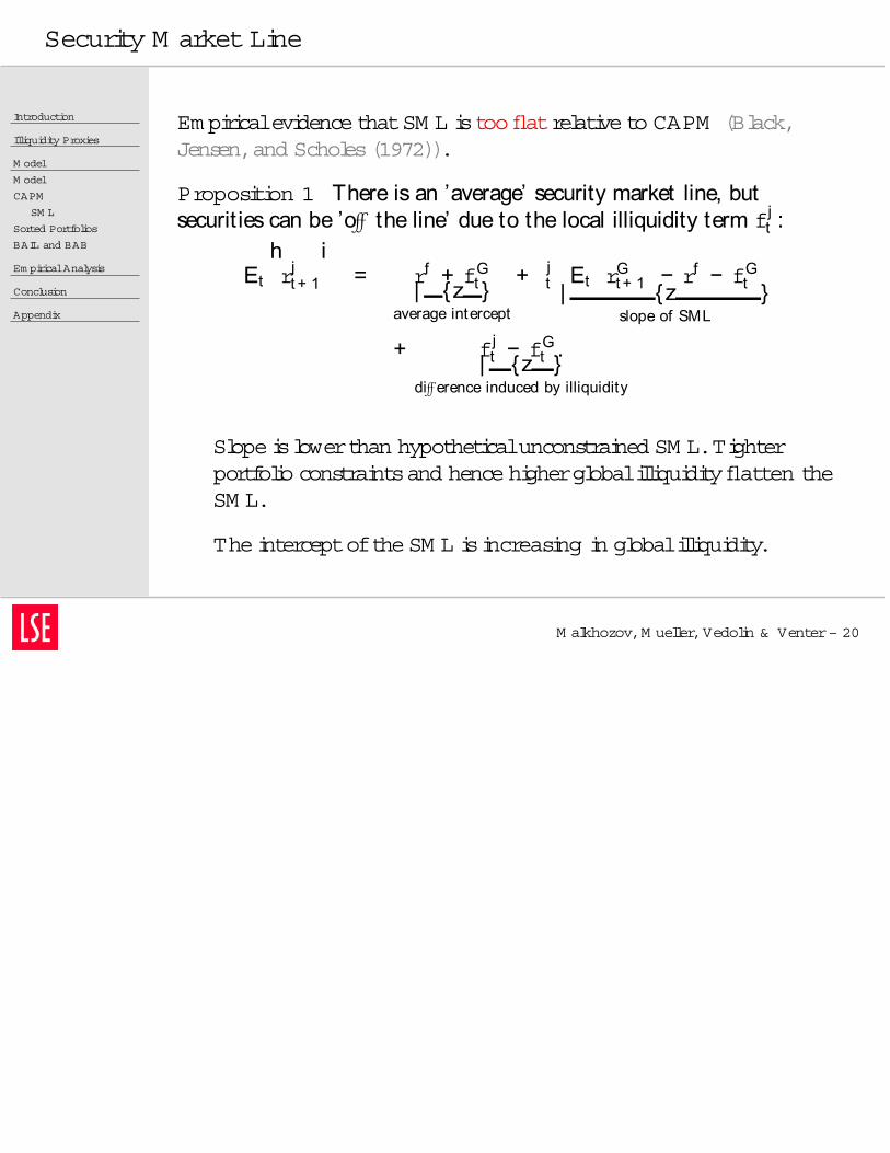
Em piricalevidencethatSM L istoo flatrelativeto CAPM (Black,Jensen,and Scholes(1972)).
Proposition 1 There is an ’average’ security market line, butsecurit ies can be ’off the line’ due to the local illiquidity term fj
t :
Et
hrj
t + 1
i= rf + fG
t| z average intercept
+ jt
Et
rG
t + 1
− rf − fG
t
| z slope of SML
+ fjt − fG
t .| z
diff erence induced by illiquidity
Slopeislowerthan hypotheticalunconstrained SM L.Tighterportfolio constraintsand hencehigherglobalilliquidity flatten theSM L.
TheinterceptoftheSM L isincreasing in globalilliquidity.
Sorted Portfoliosand Illiquidity
Introduction
Illiquidity Proxies
M odel
M odel
CAPM
SM L
Sorted Portfolios
BAIL and BAB
Em piricalAnalysis
Conclusion
Appendix
M alkhozov,M ueller,Vedolin & Venter– 21
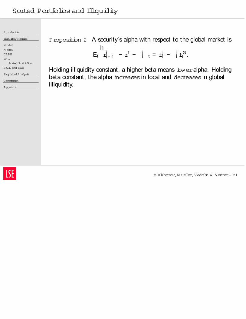
Proposition 2 A security’s alpha with respect to the global market is
Et
hrj
t + 1
i− rf − j
t t = fjt −
jt f
Gt .
Holding illiquidity constant, a higher beta means loweralpha. Holdingbeta constant, the alpha increases in local and decreases in globalilliquidity.

Self-Financing Portfolios
Introduction
Illiquidity Proxies
M odel
M odel
CAPM
SM L
Sorted Portfolios
BAIL and BAB
Em piricalAnalysis
Conclusion
Appendix
M alkhozov,M ueller,Vedolin & Venter– 22
How can (unconstrained)investorsm akem oney locally and globally?

Self-Financing Portfolios
Introduction
Illiquidity Proxies
M odel
M odel
CAPM
SM L
Sorted Portfolios
BAIL and BAB
Em piricalAnalysis
Conclusion
Appendix
M alkhozov,M ueller,Vedolin & Venter– 22
How can (unconstrained)investorsm akem oney locally and globally?
W econstructtwo self-financing m arket-neutralportfolios:
1. Betting-against-Beta (BAB):Go long thelow-beta portfolioshortthehigh-beta portfolio.
rBABt + 1 =1L Bt
rL B
t + 1 − rf−
1H Bt
rH B
t + 1 − rf
2. Beta-Adjusted-International-Illiquidity (BAIL):Go long aportfolio ofassetswith high fj
t /jt and shorta portfolio ofassets
with low fjt /
jt .Theform erhasa beta of
H and thelatterhasabeta of L .
rBAILt + 1 =1Ht
rH
t + 1 − rf−
1Lt
rL
t + 1 − rf.
Theexcessreturn ofthisportfolio is
EtrBAILt + 1
=fH
tHt−fL
tLt≥ 0
Beta Arbitrage and Illiquidity
Introduction
Illiquidity Proxies
M odel
M odel
CAPM
SM L
Sorted Portfolios
BAIL and BAB
Em piricalAnalysis
Conclusion
Appendix
M alkhozov,M ueller,Vedolin & Venter– 23
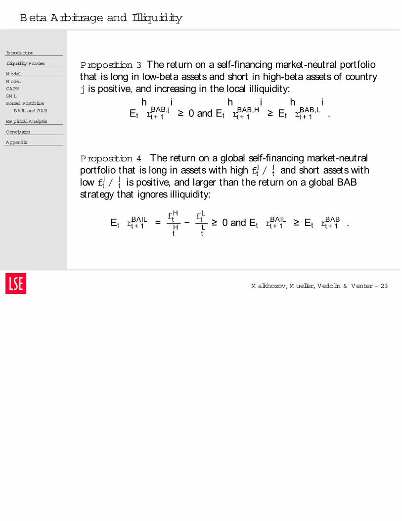
Proposition 3 The return on a self-financing market-neutral portfoliothat is long in low-beta assets and short in high-beta assets of countryj is posit ive, and increasing in the local illiquidity:
Et
hrBAB,j
t + 1
i≥ 0 and Et
hrBAB,H
t + 1
i≥ Et
hrBAB,L
t + 1
i.
Proposition 4 The return on a global self-financing market-neutralportfolio that is long in assets with high fj
t /jt and short assets with
low fjt /
jt is posit ive, and larger than the return on a global BAB
strategy that ignores illiquidity:
EtrBAIL
t + 1
=fH
tHt−fL
tLt≥ 0 and Et
rBAIL
t + 1
≥ Et
rBAB
t + 1
.
Em piricalAnalysis
Introduction
Illiquidity Proxies
M odel
Em piricalAnalysis
SM L
Sorted Pf
CAPM Alpha
BAIL vsBAB
Literature
Conclusion
Appendix
M alkhozov,M ueller,Vedolin & Venter– 24

Stock D ata and Equity Beta
Introduction
Illiquidity Proxies
M odel
Em piricalAnalysis
SM L
Sorted Pf
CAPM Alpha
BAIL vsBAB
Literature
Conclusion
Appendix
M alkhozov,M ueller,Vedolin & Venter– 25
Daily stock returns,volum e,and m arketcapitalization forthesixcountries.Theinitialsam plecoversm orethan 10k stocks.
Estim ateex-antebetasforany stock i:
ˆ TSi = ˆ
ˆ i
m,
wherethevolatilitiesarecalculated using a 1-yearwindow andcorrelationsareestim ated overa fiveyearwindow.
Finally,to accountforextrem ebeta estim atesdueto noiseandbiaseswhen wesorton beta,wefollow Vasicek (1973)by shrinkingbetastoward theircross-sectionalm ean,which issetto 1:
ˆi = 0.6 × ˆ TS
i + 0.4 × 1.
Prediction 1: Security M arketLine
Introduction
Illiquidity Proxies
M odel
Em piricalAnalysis
SM L
Sorted Pf
CAPM Alpha
BAIL vsBAB
Literature
Conclusion
Appendix
M alkhozov,M ueller,Vedolin & Venter– 26
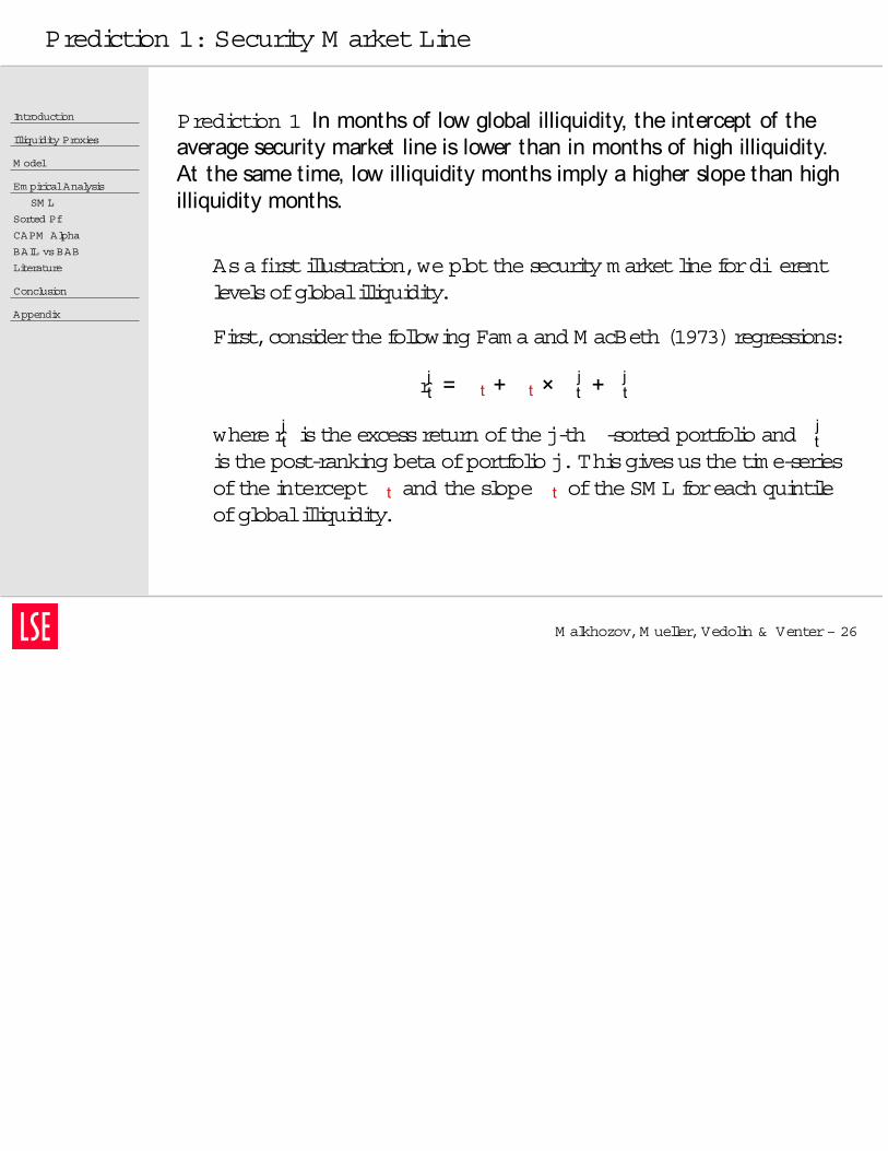
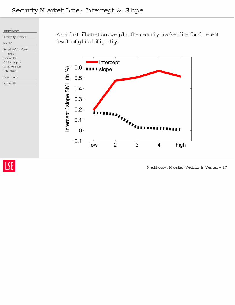
Prediction 1 In months of low global illiquidity, the intercept of theaverage security market line is lower than in months of high illiquidity.At the same time, low illiquidity months imply a higher slope than highilliquidity months.
Asa firstillustration,we plotthesecurity m arketlinefordi erentlevelsofglobalilliquidity.
First,considerthefollowing Fam aand M acBeth (1973)regressions:
rjt = t + t × jt + j
t
whererjt istheexcessreturn ofthej-th -sorted portfolio and jt
isthepost-ranking beta ofportfolio j.Thisgivesusthetim e-seriesoftheintercept t and theslope t oftheSM L foreach quintileofglobalilliquidity.
Security M arketLine: Intercept& Slope
Introduction
Illiquidity Proxies
M odel
Em piricalAnalysis
SM L
Sorted Pf
CAPM Alpha
BAIL vsBAB
Literature
Conclusion
Appendix
M alkhozov,M ueller,Vedolin & Venter– 27
Asa firstillustration,we plotthesecurity m arketlinefordi erentlevelsofglobalilliquidity.
low 2 3 4 high−0.1
0
0.1
0.2
0.3
0.4
0.5
0.6in
terc
ept /
slo
pe S
ML
(in %
)
interceptslope
Security M arketLine Regression Results
M alkhozov,M ueller,Vedolin & Venter– 28
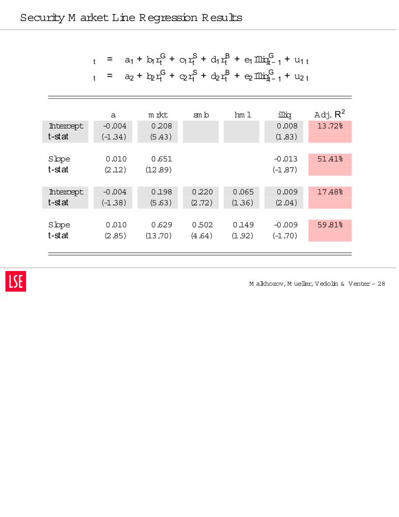
t = a1 + b1rGt + c1r
St + d1r
Bt + e1Illiq
Gt− 1 + u1t
t = a2 + b2rGt + c2r
St + d2r
Bt + e2Illiq
Gt− 1 + u2t
a m rkt sm b hm l illiq Adj.R2
Intercept -0.004 0.208 0.008 13.72%t-stat (-1.34) (5.43) (1.83)
Slope 0.010 0.651 -0.013 51.41%t-stat (2.12) (12.89) (-1.87)
Intercept -0.004 0.198 0.220 0.065 0.009 17.48%t-stat (-1.38) (5.63) (2.72) (1.36) (2.04)
Slope 0.010 0.629 0.502 0.149 -0.009 59.81%t-stat (2.85) (13.70) (4.64) (1.92) (-1.70)
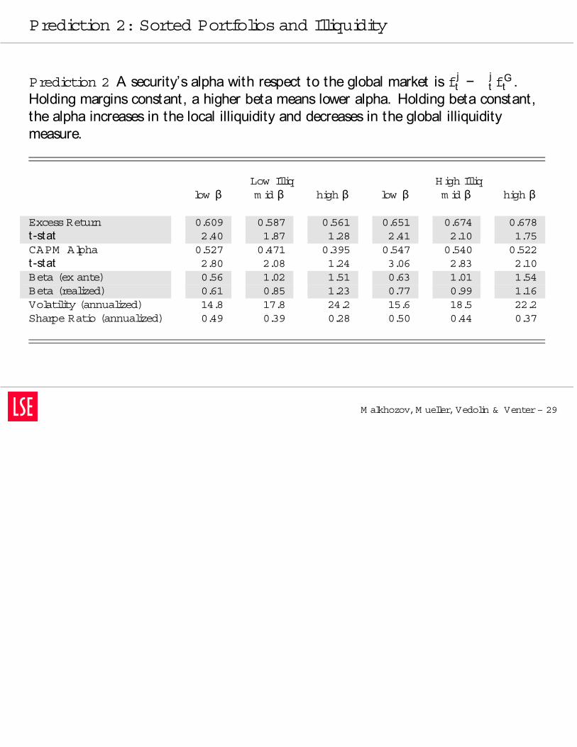
Prediction 2: Sorted Portfoliosand Illiquidity
M alkhozov,M ueller,Vedolin & Venter– 29
Prediction 2 A security’s alpha with respect to the global market is fjt −
jt f
Gt .
Holding margins constant, a higher beta means lower alpha. Holding beta constant,the alpha increases in the local illiquidity and decreases in the global illiquiditymeasure.
Low Illiq High Illiqlow β m id β high β low β m id β high β
ExcessReturn 0.609 0.587 0.561 0.651 0.674 0.678t -stat 2.40 1.87 1.28 2.41 2.10 1.75CAPM Alpha 0.527 0.471 0.395 0.547 0.540 0.522t -stat 2.80 2.08 1.24 3.06 2.83 2.10Beta (ex ante) 0.56 1.02 1.51 0.63 1.01 1.54Beta (realized) 0.61 0.85 1.23 0.77 0.99 1.16Volatility (annualized) 14.8 17.8 24.2 15.6 18.5 22.2Sharpe Ratio (annualized) 0.49 0.39 0.28 0.50 0.44 0.37
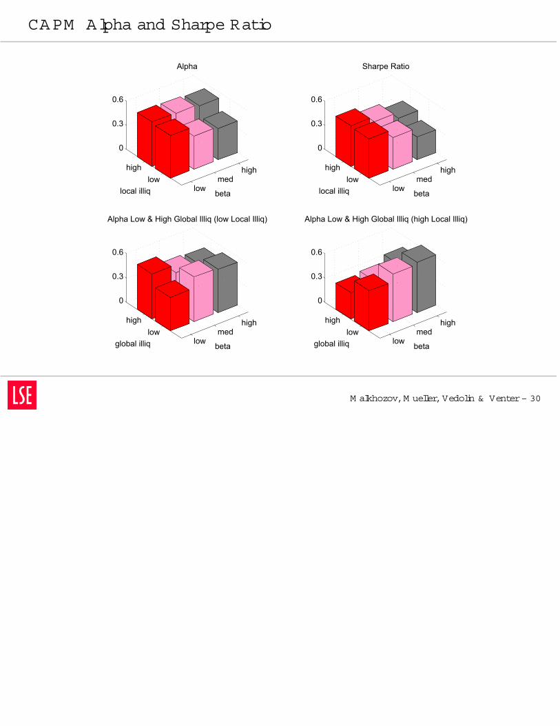
CAPM Alpha and Sharpe Ratio
M alkhozov,M ueller,Vedolin & Venter– 30
lowmed
highhigh
low
0
0.3
0.6
beta
Alpha
local illiq lowmed
highhigh
low
0
0.3
0.6
beta
Sharpe Ratio
local illiq
lowmed
highhigh
low
0
0.3
0.6
beta
Alpha Low & High Global Illiq (high Local Illiq)
global illiqlowmed
highhigh
low
0
0.3
0.6
beta
Alpha Low & High Global Illiq (low Local Illiq)
global illiq
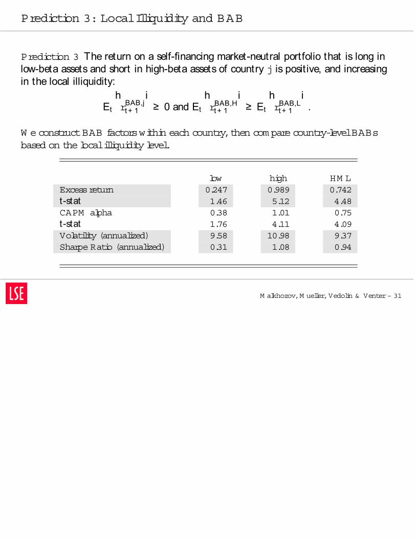
Prediction 3: LocalIlliquidity and BAB
M alkhozov,M ueller,Vedolin & Venter– 31
Prediction 3 The return on a self-financing market-neutral portfolio that is long inlow-beta assets and short in high-beta assets of country j is posit ive, and increasingin the local illiquidity:
Et
hrBAB,j
t + 1
i≥ 0 and Et
hrBAB,H
t + 1
i≥ Et
hrBAB,L
t + 1
i.
W econstructBAB factorswithin each country,then com parecountry-levelBABsbased on thelocalilliquidity level.
low high HM LExcessreturn 0.247 0.989 0.742t-stat 1.46 5.12 4.48CAPM alpha 0.38 1.01 0.75t-stat 1.76 4.11 4.09Volatility (annualized) 9.58 10.98 9.37Sharpe Ratio (annualized) 0.31 1.08 0.94
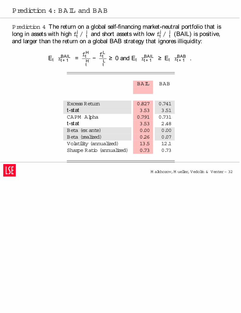
Prediction 4: BAIL and BAB
M alkhozov,M ueller,Vedolin & Venter– 32
Prediction 4 The return on a global self-financing market-neutral portfolio that islong in assets with high fj
t /jt and short assets with low fj
t /jt (BAIL) is positive,
and larger than the return on a global BAB strategy that ignores illiquidity:
EtrBAIL
t + 1
=fH
tHt−fL
tLt≥ 0 and Et
rBAIL
t + 1
≥ Et
rBAB
t + 1
.
BAIL BAB
ExcessReturn 0.827 0.741t-stat 3.53 3.51CAPM Alpha 0.791 0.731t-stat 3.53 2.48Beta (ex ante) 0.00 0.00Beta (realized) 0.26 0.07Volatility (annualized) 13.5 12.1Sharpe Ratio (annualized) 0.73 0.73
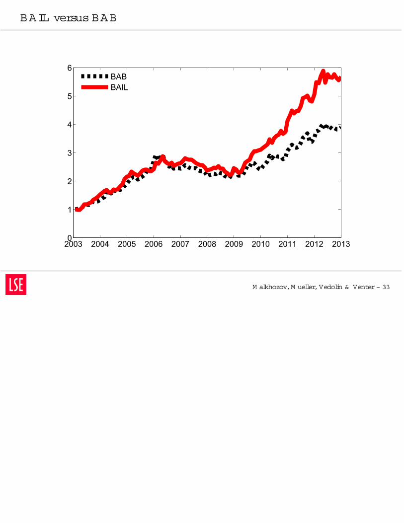
BAIL versus BAB
M alkhozov,M ueller,Vedolin & Venter– 33
2003 2004 2005 2006 2007 2008 2009 2010 2011 2012 20130
1
2
3
4
5
6
BABBAIL
BAIL versus BAB (cont.)
Introduction
Illiquidity Proxies
M odel
Em piricalAnalysis
SM L
Sorted Pf
CAPM Alpha
BAIL vsBAB
Literature
Conclusion
Appendix
M alkhozov,M ueller,Vedolin & Venter– 34
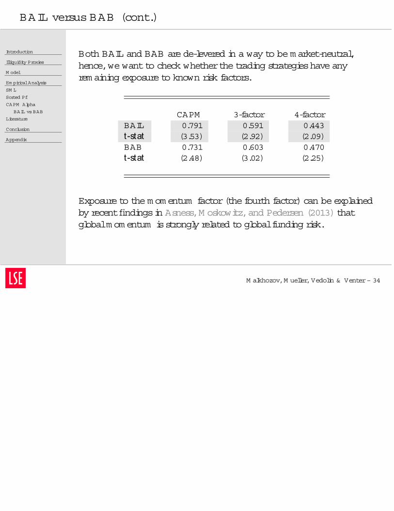
Both BAIL and BAB arede-levered in a way to bem arket-neutral,hence,we wantto check whetherthetrading strategieshaveanyrem aining exposureto known risk factors.
CAPM 3-factor 4-factorBAIL 0.791 0.591 0.443t-stat (3.53) (2.92) (2.09)BAB 0.731 0.603 0.470t-stat (2.48) (3.02) (2.25)
Exposureto them om entum factor(thefourth factor)can beexplainedby recentfindingsin Asness,M oskowitz,and Pedersen (2013)thatglobalm om entum isstrongly related to globalfunding risk.
Literature
Introduction
Illiquidity Proxies
M odel
Em piricalAnalysis
SM L
Sorted Pf
CAPM Alpha
BAIL vsBAB
Literature
Conclusion
Appendix
M alkhozov,M ueller,Vedolin & Venter– 35
Funding constraints & assetprices:
Xiong (2001),Kyleand Xiong (2001),Grom b and Vayanos(2002,2012),Krishnam urthy(2003),Brunnerm eierand Pedersen (2009),Garleanu and Pedersen (2011),Frazziniand Pedersen (2013).
Liquidity risk & internationalstock returns:
Bekaert,Harvey,and Lundblad (2007),Lee(2011),Karolyi,Lee,andvan Dijk (2012),Am ihud,Ham eed,Kang,and Zhang (2013).
InternationalFinance,portfolio constraints & segm entation:
Black (1974),Stulz(1981),Errunza and Losq (1985,1989),Eun andJarakiram anan (1986),Hietala (1989),Pavlova and Rigobon (2007)
Conclusion
Introduction
Illiquidity Proxies
M odel
Em piricalAnalysis
Conclusion
Conclusion
Appendix
M alkhozov,M ueller,Vedolin & Venter– 36
Conclusion
Introduction
Illiquidity Proxies
M odel
Em piricalAnalysis
Conclusion
Conclusion
Appendix
M alkhozov,M ueller,Vedolin & Venter– 37
Thispaperstudiesa world econom y whereagentsaresubjecttoagent-and country-specificm argin constraints,and deriveaninternationalfunding-liquidityadjusted CAPM whereexpectedreturnsnotonlydepend on theglobalm arketrisk ofassetsbutalsoon localand globalilliquidity m easures.
Higherilliquidity⇒ Higherinterceptand lowerslopeofSM L.
Higherilliquidity⇒ Higheralpha and Sharperatio.
M arket-neutralBAIL strategyproducessignificantabnorm alreturnswith a Sharperatio of0.73 and outperform sa standard BABstrategy.
Conclusion
Introduction
Illiquidity Proxies
M odel
Em piricalAnalysis
Conclusion
Conclusion
Appendix
M alkhozov,M ueller,Vedolin & Venter– 37
Thispaperstudiesa world econom y whereagentsaresubjecttoagent-and country-specificm argin constraints,and deriveaninternationalfunding-liquidityadjusted CAPM whereexpectedreturnsnotonlydepend on theglobalm arketrisk ofassetsbutalsoon localand globalilliquidity m easures.
Higherilliquidity⇒ Higherinterceptand lowerslopeofSM L.
Higherilliquidity⇒ Higheralpha and Sharperatio.
M arket-neutralBAIL strategyproducessignificantabnorm alreturnswith a Sharperatio of0.73 and outperform sa standard BABstrategy.
Thank you very m uch foryourattention!

Appendix
Introduction
Illiquidity Proxies
M odel
Em piricalAnalysis
Conclusion
Appendix
Com parison Global
Com parison Am ihud
Com parison VIX
Em bedded Leverage
M alkhozov,M ueller,Vedolin & Venter– 38
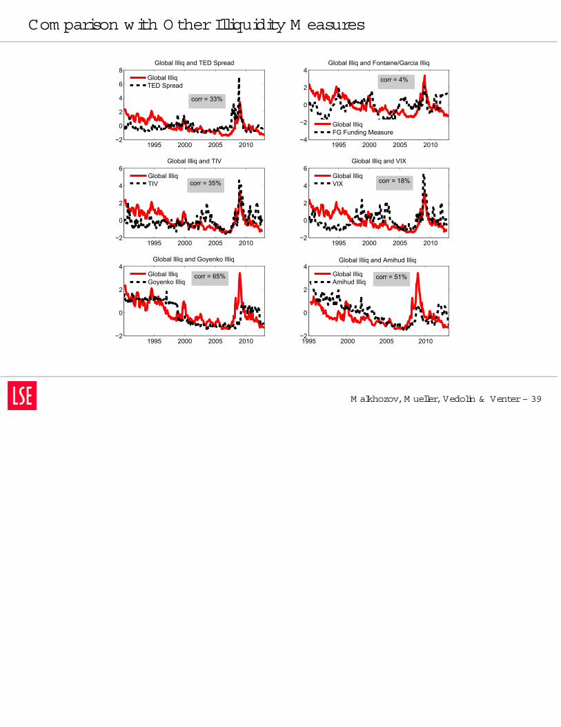
Com parison with O therIlliquidity M easures
M alkhozov,M ueller,Vedolin & Venter– 39
1995 2000 2005 2010−2
0
2
4
6
8Global Illiq and TED Spread
Global IlliqTED Spread
1995 2000 2005 2010−4
−2
0
2
4Global Illiq and Fontaine/Garcia Illiq
Global IlliqFG Funding Measure
1995 2000 2005 2010−2
0
2
4
6Global Illiq and TIV
Global IlliqTIV
1995 2000 2005 2010−2
0
2
4
6Global Illiq and VIX
Global IlliqVIX
1995 2000 2005 2010−2
0
2
4Global Illiq and Goyenko Illiq
Global IlliqGoyenko Illiq
1995 2000 2005 2010−2
0
2
4Global Illiq and Amihud Illiq
Global IlliqAmihud Illiq
corr = 33%
corr = 4%
corr = 35% corr = 18%
corr = 65% corr = 51%
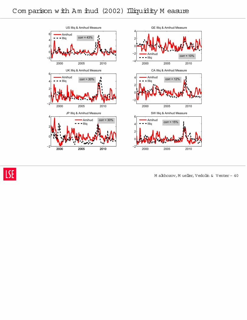
Com parison with Am ihud (2002) Illiquidity M easure
M alkhozov,M ueller,Vedolin & Venter– 40
2000 2005 2010
−2
0
2
4
6
US Illiq & Amihud Measure
AmihudIlliq
2000 2005 2010−4
−2
0
2
4GE Illiq & Amihud Measure
AmihudIlliq
2000 2005 2010−2
0
2
4
6UK Illiq & Amihud Measure
AmihudIlliq
2000 2005 2010
−2
0
2
4
CA Illiq & Amihud Measure
AmihudIlliq
2000 2005 2010−2
0
2
4
6SW Illiq & Amihud Measure
AmihudIlliq
2000 2005 2010−2
0
2
4JP Illiq & Amihud Measure
2000 2005 2010
AmihudIlliq
corr = 43%
corr = 10%
corr = 30% corr = 12%
corr = 15%corr = 30%
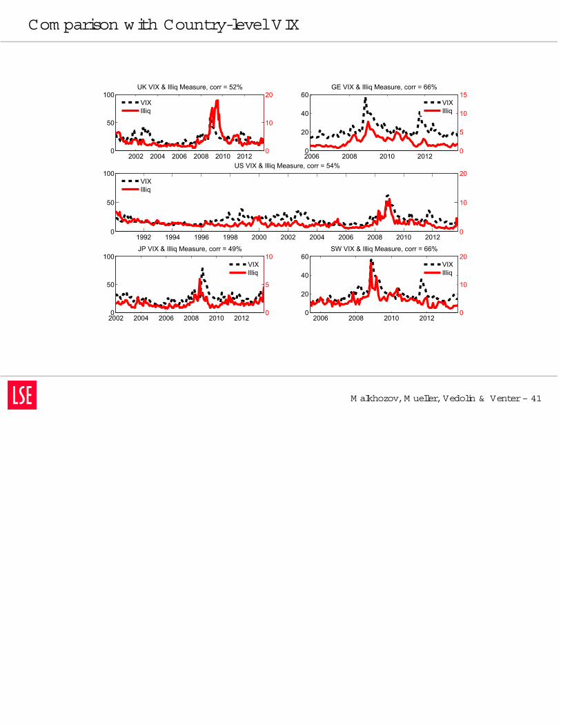
Com parison with Country-levelVIX
M alkhozov,M ueller,Vedolin & Venter– 41
1992 1994 1996 1998 2000 2002 2004 2006 2008 2010 20120
50
100US VIX & Illiq Measure, corr = 54%
0
10
20VIXIlliq
2006 2008 2010 20120
20
40
60GE VIX & Illiq Measure, corr = 66%
0
5
10
15VIXIlliq
2002 2004 2006 2008 2010 20120
50
100UK VIX & Illiq Measure, corr = 52%
0
10
20VIXIlliq
2002 2004 2006 2008 2010 20120
50
100JP VIX & Illiq Measure, corr = 49%
0
5
10VIXIlliq
2006 2008 2010 20120
20
40
60SW VIX & Illiq Measure, corr = 66%
0
10
20VIXIlliq
LetThem Buy ETFs orO ptions!
Introduction
Illiquidity Proxies
M odel
Em piricalAnalysis
Conclusion
Appendix
Com parison Global
Com parison Am ihud
Com parison VIX
Em bedded Leverage
M alkhozov,M ueller,Vedolin & Venter– 42
Argum entthatpeoplewho wantleveragecan sim ply buy optionsorETFs.Butthey deliverlow expected returns(FrazziniandPedersen (2012)):
Intuition:Em bedded leveragealleviatesinvestors’leverageconstraints,and thereforeassetswith em bedded leverageyieldlowerexpected returns.
A portfolio which islong low-em bedded-leveragesecuritiesandshorthigh-em bedded-leveragesecuritiesearnslargeabnorm alreturns,with t-statisticsof8.6 forequity options,6.3 forindexoptionsand 2.5 forETFs.
Recommended