Download pdf - Pressure Transient Solutions for Vertically Slotted ... · Pressure Transient Solutions for Vertically Slotted-Partially Penetrated Vertical ... well testing and Wireline formation

Transp Porous Med (2015) 106:455–486DOI 10.1007/s11242-014-0410-8

Pressure Transient Solutions for VerticallySlotted-Partially Penetrated Vertical Wellsin Porous Media

Denis Biryukov · Fikri J. Kuchuk

Received: 6 December 2013 / Accepted: 22 October 2014 / Published online: 8 November 2014© The Author(s) 2014. This article is published with open access at Springerlink.com

Abstract In this paper, we present semi-analytical pressure transient solutions for verticallyslotted-limited entry or partially penetrated vertical wells. These solutions are needed forinterpretation of the pressure transient tests conducted with the Wireline Formation Testingvertically slotted-packer configuration, and in wells with vertically slotted-liner completions.These slots have limited size openings and are vertically placed on a non-permeable cylin-drical wellbore in a porous medium. The fluid from the formation is produced through theseslots into the wellbore. Pressure transient solutions are not readily available for the uniformpressure boundary condition on the surface of the slots because such a condition creates amixed boundary value problem, which is difficult to solve. Here we present exact pressuretransient solutions obtained under the assumption that the pressure on the slot surface isuniform but a priori unknown, and the rest of the wellbore surface is non-permeable (no-flowcondition). Furthermore, we generalize our solution for the case of multiple slots (open sec-tions) on the wellbore for both well testing and Wireline formation tester packer modules.Our solutions are compared with the existing solutions. A new formula for obtaining thedrawdown horizontal mobility is presented for anisotropic media.

Keywords Pressure transient solutions · Slotted-partially penetrated vertical wells ·Pressure transient testing · Slotted dual-packer module · Mobility estimation

List of Symbols

C Wellbore storage constant, RB/psi (m3/Pa)c Compressibility, psi−1 (Pa−1)

se & ce Normalized angular even and odd Mathieu functionserf Error functionh Formation thickness, ft [m]

D. Biryukov · F. J. Kuchuk (B)1 rue Henri Becquerel, 92142 Clamart Cedex, Francee-mail: [email protected]

123

456 D. Biryukov, F. J. Kuchuk

g Unit impulse responseI Modified Bessel function of the first kindJ Bessel function of the first kindK Modified Bessel function of the second kindk Permeability, md (m2)

l Characteristic length or Half-length, ft (m)L Laplace transformL−1 Inverse Laplace transformMc & Ms Radial even and odd Mathieu functions of the third kindp Pressure, psi (Pa)q flow rate, RB/D (m3/s)r Radius or radial coordinates Laplace transform variableT Chebyshev polynomialt Time, h (s)x Coordinatey Coordinatez Vertical coordinateα Constantβ Constantγ Constantδ Constantη Diffusivity for pressureμ Viscosity, cp (Pa s)φ Porosity, fractionτ Dummy variableξ Dummy variable

Subscripts

a Pressure-averagedD Dimensionlessf Formationh Horizontalm Measuredo Initial or originals f Sandfaceu Uniform pressurev Verticalw Wellbore

1 Introduction

Pressure transient tests are conducted along the wellbore to obtain reservoir pressure and adiscrete permeability (horizontal and vertical permeabilities) distribution with the wirelineformation testers (WFT), shown in Fig. 1 (Kuchuk et al. 2010; Zimmerman et al. 1990). Awireline formation tester consists of a number of modules and allows an unlimited number of

123

Pressure Transient Solutions in Porous Media 457

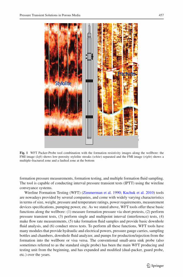
Fig. 1 WFT Packer-Probe tool combination with the formation resistivity images along the wellbore: theFMI image (left) shows low-porosity stylolite streaks (white) separated and the FMI image (right) shows amultiple-fractured zone and a faulted zone at the bottom

formation pressure measurements, formation testing, and multiple formation fluid sampling.The tool is capable of conducting interval pressure transient tests (IPTT) using the wirelineconveyance systems.

Wireline Formation Testing (WFT) (Zimmerman et al. 1990; Kuchuk et al. 2010) toolsare nowadays provided by several companies, and come with widely varying characteristicsin terms of size, weight, pressure and temperature ratings, power requirements, measurementdevices specifications, pumping power, etc. As we stated above, WFT tools offer these basicfunctions along the wellbore: (1) measure formation pressure via short pretests, (2) performpressure transient tests, (3) perform single and multipoint interval (interference) tests, (4)make flow rate measurements, (5) take formation fluid samples and provide basic downholefluid analysis, and (6) conduct stress tests. To perform all these functions, WFT tools havemany modules that provide hydraulic and electrical powers, pressure gauge carries, samplingbottles and chambers, downhole fluid analyzer, and pumps for production/injection from theformation into the wellbore or visa versa. The conventional small-area sink probe (alsosometimes referred to as the standard single probe) has been the main WFT producing andtesting unit from the beginning, and has expanded and modified (dual-packer, guard probe,etc.) over the years.

123


For the purpose of pretests and pressure transient testing, the most important components ofa WFT string are the probes or dual-packers (Fig. 1) through which the flow from the formationinto the tool string takes place, and where both pressure and flow rate are recorded. Differenttypes of probes and dual-packers exist and can be assembled in different ways. Beyond theseessential elements, other modules also are necessary to perform the flow operations, such aspumps, power modules, sample chambers, etc. The packer module has two packer elementsthat are inflated to isolate about 1 m (3.3 ft) wellbore interval, as shown in Fig. 1. Becausea large section of the sandface is open to flow between two packer elements, the productioninterval of the formation is several thousand times larger than that of conventional probes.Unlike the flow geometry of conventional probes, the radial symmetry about the wellboreaxis is maintained with the dual-packer geometry during the flow in laterally anisotropichomogenous reservoirs, and is slightly distorted in vertically anisotropic systems. Therefore,the dual-packer module is very useful for conducting pressure transient tests in heterogeneous,layered, shaly, fractured, and vuggy formations. In these type of formations, it is not difficultto sustain the hydraulic isolation of the tested section from the rest of the wellbore, particularlyin fractured and vuggy formations. As shown in Fig. 1, the dual-packer envelops a matrix,fracture and/or fault zone and is set against the borehole wall to hydraulically isolate thetested section, see for instance, Zeybek et al. (2002) for the details of packer-probe transienttests that are conducted across the fracture zones.

The dual-packer module is also very useful for WFT testing of unconsolidated formationsand condensate reservoirs because the packer production area of the sandface several thousandtimes larger than the production area of conventional probes (Kuchuk et al. 2010). In otherwords, the wellbore pressure drop is very small during transient tests and sampling with theparker module compared to that of conventional probes even though production rate couldbe usually much higher for the parker module. It is well known that the sand production intothe wellbore is extremely sensitive to the pressure drop during WFT testing and sampling ofunconsolidated formations. Condensate reservoirs are also extremely sensitive to the pressurechange. If the wellbore pressure drops below the dewpoint during testing and sampling, liquidcondenses from gas and form a condensate bank, which highly complicates both testing andsampling.

In some respects, a dual-packer pressure transient test resembles a small scale DST-typetest, although the radius of investigation of a dual-packer pressure transient test is not morethan a few tens of feet (10–50 ft). A longer production time will increase the radius ofinvestigation very little because a spherical flow is established in the vicinity of the wellboredue to a small-length production interval, unless the formation is thin. The dual-packermodule with one or two probes is also very useful for permeability profiling along thewellbore, particularly in layered reservoirs. For instance, as shown in Fig. 1, the FMI image(left) shows three low-porosity stylolite streaks (white) separated by dark very permeableintervals. The top stylolite streak is particularly patchy. Usually, the stylolite intervals may bethinner than 1 ft, therefore, conventional probes are not suitable to test these stylolite zones.The same figure also shows the FMI image (right), where a multiple-fractured zone and afaulted zone at the bottom can be observed. Again conventional probes are not suitable totest these fractured and faulted zones.

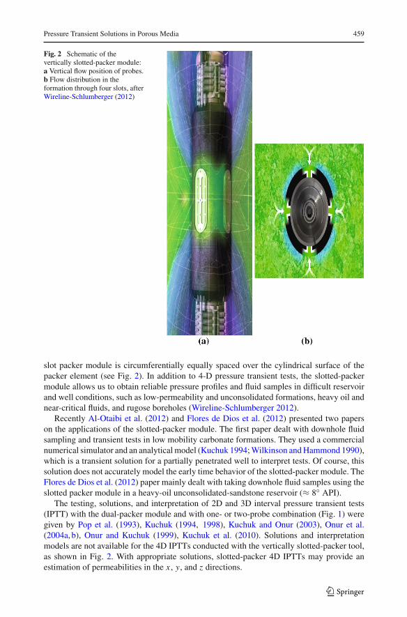
The recently introduced vertically slotted-packer probe (Saturn1 3D radial packer module),as shown in Fig. 2, provides a new type of 4-Dimensional pressure transient test data. Asshown in Fig. 3, the packer has four rectangular slots with a height of 188 mm (0.6168 ft)and a width of 74.5 mm (0.2444 ft). The tips of each slot are slightly oval-shaped. The four

1 Mark of Schlumberger.

123


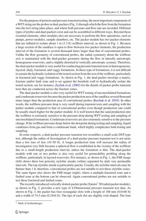
Fig. 2 Schematic of thevertically slotted-packer module:a Vertical flow position of probes.b Flow distribution in theformation through four slots, afterWireline-Schlumberger (2012)

slot packer module is circumferentially equally spaced over the cylindrical surface of thepacker element (see Fig. 2). In addition to 4-D pressure transient tests, the slotted-packermodule allows us to obtain reliable pressure profiles and fluid samples in difficult reservoirand well conditions, such as low-permeability and unconsolidated formations, heavy oil andnear-critical fluids, and rugose boreholes (Wireline-Schlumberger 2012).

Recently Al-Otaibi et al. (2012) and Flores de Dios et al. (2012) presented two paperson the applications of the slotted-packer module. The first paper dealt with downhole fluidsampling and transient tests in low mobility carbonate formations. They used a commercialnumerical simulator and an analytical model (Kuchuk 1994; Wilkinson and Hammond 1990),which is a transient solution for a partially penetrated well to interpret tests. Of course, thissolution does not accurately model the early time behavior of the slotted-packer module. TheFlores de Dios et al. (2012) paper mainly dealt with taking downhole fluid samples using theslotted packer module in a heavy-oil unconsolidated-sandstone reservoir (≈ 8◦ API).

The testing, solutions, and interpretation of 2D and 3D interval pressure transient tests(IPTT) with the dual-packer module and with one- or two-probe combination (Fig. 1) weregiven by Pop et al. (1993), Kuchuk (1994, 1998), Kuchuk and Onur (2003), Onur et al.(2004a, b), Onur and Kuchuk (1999), Kuchuk et al. (2010). Solutions and interpretationmodels are not available for the 4D IPTTs conducted with the vertically slotted-packer tool,as shown in Fig. 2. With appropriate solutions, slotted-packer 4D IPTTs may provide anestimation of permeabilities in the x , y, and z directions.

123


Fig. 3 Schematic of thevertically slotted-packer modulewith its dimensions, where theorigin the coordinate system is onthe well axis at{x = rw, y = 0, z = 0} whichcorresponds to the center of theprobe

lw

x

y

z

Formation

Open slot:

rw

Well

∂

o

Impermeablecylindricalwellbore:

Packer module

∂

r θ

2b

lw

h

Impermeable top boundary

Impermeable bottom boundary

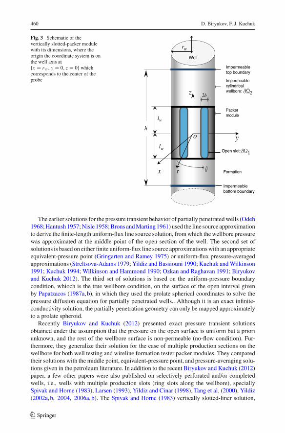
The earlier solutions for the pressure transient behavior of partially penetrated wells (Odeh1968; Hantush 1957; Nisle 1958; Brons and Marting 1961) used the line source approximationto derive the finite-length uniform-flux line source solution, from which the wellbore pressurewas approximated at the middle point of the open section of the well. The second set ofsolutions is based on either finite uniform-flux line source approximations with an appropriateequivalent-pressure point (Gringarten and Ramey 1975) or uniform-flux pressure-averagedapproximations (Streltsova-Adams 1979; Yildiz and Bassiouni 1990; Kuchuk and Wilkinson1991; Kuchuk 1994; Wilkinson and Hammond 1990; Ozkan and Raghavan 1991; Biryukovand Kuchuk 2012). The third set of solutions is based on the uniform-pressure boundarycondition, whioch is the true wellbore condition, on the surface of the open interval givenby Papatzacos (1987a, b), in which they used the prolate spherical coordinates to solve thepressure diffusion equation for partially penetrated wells.. Although it is an exact infinite-conductivity solution, the partially penetration geometry can only be mapped approximatelyto a prolate spheroid.

Recently Biryukov and Kuchuk (2012) presented exact pressure transient solutionsobtained under the assumption that the pressure on the open surface is uniform but a prioriunknown, and the rest of the wellbore surface is non-permeable (no-flow condition). Fur-thermore, they generalize their solution for the case of multiple production sections on thewellbore for both well testing and wireline formation tester packer modules. They comparedtheir solutions with the middle point, equivalent-pressure point, and pressure-averaging solu-tions given in the petroleum literature. In addition to the recent Biryukov and Kuchuk (2012)paper, a few other papers were also published on selectively perforated and/or completedwells, i.e., wells with multiple production slots (ring slots along the wellbore), speciallySpivak and Horne (1983), Larsen (1993), Yildiz and Cinar (1998), Tang et al. (2000), Yildiz(2002a, b, 2004, 2006a, b). The Spivak and Horne (1983) vertically slotted-liner solution,

123


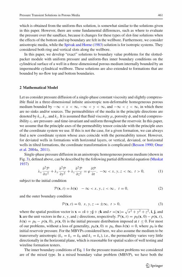
which is obtained from the uniform-flux solution, is somewhat similar to the solutions givenin this paper. However, there are some fundamental differences, such as where to evaluatethe pressure over the sandface, because it changes for these types of slot-line solutions whenthe effects of the bottom and top boundary are felt in the wellbore. Furthermore, we consideranisotropic media, while the Spivak and Horne (1983) solution is for isotropic systems. Theyconsidered both ring and vertical slots along the wellbore.

In this paper, we develop “exact” solutions to boundary value problems for the slotted-packer module with uniform pressure and uniform-flux inner boundary conditions on thecylindrical surface of a well in a three-dimensional porous medium internally bounded by animpermeable cylindrical wellbore. These solutions are also extended to formations that arebounded by no-flow top and bottom boundaries.

2 Mathematical Model

Let us consider pressure diffusion of a single-phase constant viscosity and slightly compress-ible fluid in a three-dimensional infinite anisotropic non-deformable homogeneous porousmedium bounded by −∞ < x < ∞, −∞ < y < ∞, and −∞ < z < ∞, in which thereare no sinks and/or sources. The permeabilities of the media in the principle directions aredenoted by kx , ky , and kz . It is assumed that fluid viscosityμ, porosity φ, and total compress-ibility ct are pressure- and time-invariant and uniform throughout the reservoir. In this paper,we assume that the principle axes of the permeability tensor coincide with the principle axesof the coordinate system we use. If this is not the case, for a given formation, we can alwaysfind a new coordinate system whose axes coincide with the permeability tensor. However,for deviated wells in formations with horizontal layers, or vertical, deviated, or horizontalwells in tilted formations, the coordinate transformation is complicated (Besson 1990; Onuret al. 2004a, 2011).

Single-phase pressure diffusion in an anisotropic homogeneous porous medium (shown inFig. 3), defined above, can be described by the following partial differential equation (Muskat1937)

λx∂2P∂x2 + λy

∂2P∂y2 + λz

∂2P∂z2 = ϕ

∂P∂t, −∞ < x, y, z < ∞, t > 0, (1)

subject to the initial condition

P(x, t) = h(x) − ∞ < x, y, z < ∞ , t = 0, (2)

and the outer boundary condition

P(x, t) = 0, x, y, z → ±∞, t > 0, (3)

where the spatial position vector is x = x i + yj + zk and r =|x |= √x2 + y2 + z2, i, j, andk are the unit vectors in the x , y, and z directions, respectively. P(x, t) = p0(x, 0)− p(x, t),h(x) = p0 − p(x, 0), p(x, 0) is the initial pressure distribution imposed at t ≤ 0. For mostof our problems, without a loss of generality, p0(x, 0) ≡ p0, thus h(x) = 0, where p0 is theinitial reservoir pressure. For the MBVPs considered here, we also assume the medium to betransversely anisotropic (kx = ky = kh and kz = kv), i.e., the permeability varies very littledirectionally in the horizontal plane, which is reasonable for spatial scales of well testing andwireline formation testers.

The inner boundary conditions of Eq. 1 for the pressure transient problems we consideredare of the mixed type. In a mixed boundary value problem (MBVP), we have both the

123


Neumann and Dirichlet boundary conditions imposed on the inner boundary surface. Forinstance, as shown in Fig. 3, the boundary condition at the open (producing) section of theinner boundary ∂Ω1, for which the total volumetric flow rate q is specified, can be written as

−∫∫

∂Ω1

{n · T grad [P(x, t)]} dS = q(t) on ∂Ω1, t > 0, (4)

where n is the outer normal vector to the surface ∂Ω1, T is the mobility tensor, q is the totalflux outwards from the surface ∂Ω1, and for the no-flow section of the inner boundary

{n · T grad [P(x, t)]} = 0 on ∂Ω2, t > 0. (5)

Furthermore, we also require the pressure (potential) at the open surface ∂Ω1 to be uniform(independent of x), which implies that

P(x, t) = Pwu(t) on ∂Ω1, t > 0. (6)

The inner boundary conditions specified by Eqs. 4–6 over the surfaces ∂Ω1 and ∂Ω2 createa mixed boundary value problem.

In this paper, we will present solutions for the constant sandface flow rate (qs f ). If the flowrate varies, then wellbore pressure at any time can be written from the convolution integral(Muskat 1937), which is Duhamel’s superposition principle, as

pw(t) = po −t∫

0

qs f (τ ) gw (t − τ) dτ (7)

and in the Laplace domain

pw(s) = po

s− qs f (s)gw(s), (8)

where t is time and gw is the impulse response at the wellbore. If the flow rate is constant atthe surface, the wellbore pressure, including skin and storage effects in the Laplace domain,can be written from Eq. 8 (see pages 60–66 of Kuchuk et al. (2010) for the details) as

pw(s) = po

s− qgw(s)

s [1 + Csgw(s)]. (9)

Equation 9 in terms of the dimensionless wellbore impulse response can be written as

pwD(s) = gwD(s)

1 + CDsgwD(s), (10)

and in terms of the dimensionless pressure and skin (S) as

pwD(sD) = s pD(s)+ S

s {1 + CDs [s pD(s)+ S]} , (11)

where

pwD = 4πkhlwΔpwqμ

, tD = kht

φμctr2w

, CD = C

2πφct hr2w

, (12)

C is the wellbore storage coefficient, S is the skin factor, and s is the Laplace transformvariable that is related to the dimensionless time tD . The above equations in this sectionprovide a general framework for interpreting simultaneously measured pressure data with anarbitrarily varying flow rate as a function of time for both pressure transient well and wirelineformation testing. The dimensionless pDs for the formation pressure with the inner boundary

123


conditions of Eq. 1 will be presented in the following sections. If the flow rate is variable atthe sandface or surface, the convolution integral given by Eq. 7 and its Laplace transformgiven by Eqs. 8 should be used to obtain the wellbore pressure. Therefore, to simplify thebelow derivations, we will assume everywhere that total flow rate q(t) ≡ q is independentof time.

3 Pressure Transient Solutions for Vertical Multiple Slots (Openings) on a PartiallyPenetrated Well

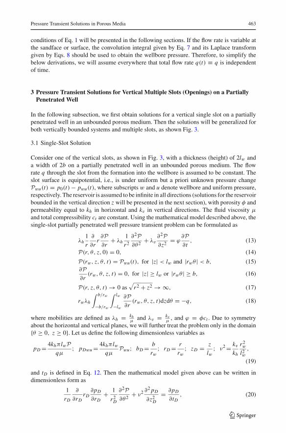
In the following subsection, we first obtain solutions for a vertical single slot on a partiallypenetrated well in an unbounded porous medium. Then the solutions will be generalized forboth vertically bounded systems and multiple slots, as shown Fig. 3.

3.1 Single-Slot Solution

Consider one of the vertical slots, as shown in Fig. 3, with a thickness (height) of 2lw anda width of 2b on a partially penetrated well in an unbounded porous medium. The flowrate q through the slot from the formation into the wellbore is assumed to be constant. Theslot surface is equipotential, i.e., is under uniform but a priori unknown pressure changePwu(t) = p0(t)− pwu(t), where subscripts w and u denote wellbore and uniform pressure,respectively. The reservoir is assumed to be infinite in all directions (solutions for the reservoirbounded in the vertical direction z will be presented in the next section), with porosity φ andpermeability equal to kh in horizontal and kv in vertical directions. The fluid viscosity μand total compressibility ct are constant. Using the mathematical model described above, thesingle-slot partially penetrated well pressure transient problem can be formulated as

λh1

r

∂

∂rr∂P∂r

+ λh1

r2

∂2P∂θ2 + λv

∂2P∂z2 = ϕ

∂P∂t, (13)

P(r, θ, z, 0) = 0, (14)

P(rw, z, θ, t) = Pwu(t), for |z| < lw and |rwθ | < b, (15)∂P∂r(rw, θ, z, t) = 0, for |z| ≥ lw or |rwθ | ≥ b, (16)

P(r, z, θ, t) → 0 as√

r2 + z2 → ∞, (17)

rwλh

∫ b/rw

−b/rw

∫ lw

−lw

∂P∂r(rw, θ, z, t)dzdθ = −q, (18)

where mobilities are defined as λh = khμ

and λv = kvμ

, and ϕ = φct . Due to symmetryabout the horizontal and vertical planes, we will further treat the problem only in the domain{θ ≥ 0, z ≥ 0}. Let us define the following dimensionless variables as

pD = 4khπlwPqμ

; pDwu = 4khπlwqμ

Pwu; bD = b

rw; rD = r

rw; zD = z

lw; ν2 = kv

kh

r2w

l2w

,

(19)

and tD is defined in Eq. 12. Then the mathematical model given above can be written indimensionless form as

1

rD

∂

∂rDrD∂pD

∂rD+ 1

r2D

∂2P∂θ2 + ν2 ∂

2 pD

∂z2D

= ∂pD

∂tD, (20)

123


pD(rD, θ, zD, 0) = 0, (21)

pD(1, θ, zD, tD) = pDwu(tD), for 0 ≤ zD < 1 and 0 ≤ θ < bD, (22)∂pD

∂rD(1, θ, zD, tD) = 0, for zD ≥ 1 or θ ≥ bD, (23)

pD(rD, θ, zD, tD) → 0 as√

r2D + z2

D → ∞, (24)

1

π

∫ bD

0

∫ 1

0

∂pD

∂rD(1, θ, zD, tD)dzD = −1. (25)

Equations 22 and 25 can be further rewritten in the following form

∂pD

∂rD(1, θ, zD, tD) = −qD(θ, zD, tD), for 0 ≤ zD < 1 and 0 ≤ θ < bD, (26)

where the function qD(θ, zD, tD) is a priori unknown and will be specified later. Using theboundary conditions given by Eqs. 23 and 26, the solution to Eq. 20 can be written as

pD(rD, θ, zD, tD) =∫ tD

0

∫ 1

0

∫ bD

0qD(ψ, u, τ )G(rD, θ, ψ, zD, u, tD − τ)dudψdτ, (27)

where G is a Green’s function for the corresponding problem which can be expressed as

G(rD, θ, ψ, zD, u, tD) = Θ(rD, θ, ψ, tD)Z(zD, u, tD), (28)

with

Θ(rD, θ, ψ, tD) = L−1

{1√s

∞∑

n=0

(1 − δ0n

2

)2Kn(rD

√s) cos(nθ) cos(nψ)

Kn+1(√

s)+ Kn−1(√

s)

}

, (29)

Z(zD, u, tD) = 2e−(zD−u)2/(4ν2tD)

√π tDν

. (30)

where

δi j ={

1 when i = j,0 when i = j.

(31)

Now let us assume that the slot flux density qD(θ, u, τ ) can be expressed as

qD(θ, u, τ ) = 1

π

∞∑

i=0

∞∑

j=0

ci j (t)(−1)i T2i (θ/bD)√

b2D − θ2

T2 j (zD)√1 − z2

D

, (32)

where T is the Chebychev polynomial and the time functions ci j will be determined later.The factor 1√

b2D−θ2

√1−z2

D

reflects the main singularity of the flux density near the slot tips

—its divergence—and insures fast convergence of the series.Substituting qD in this form into Eq. 27, we can obtain the following expression for the

dimensionless reservoir pressure:

pD(rD, θ, zD, tD) =∞∑

i=0

∞∑

j=0

∫ tD

0ci j (τ )Θ2i (rD, θ, tD − τ)Z2 j (zD, tD − τ)dτ, (33)

123


where

Θ2i (rD, θ, tD) = L−1

{1√s

∞∑

n=0

(1 − δ0n

2

)2Kn(rD

√s)J2i (nbD) cos(nθ)

Kn+1(√

s)+ Kn−1(√

s)

}

, (34)

Z2 j (zD, u, tD) = 1√π tDν

∫ π

0e−(zD−cos η)2/(4ν2tD) cos(2 jη)dη. (35)

Although these functions seem complicated, we will show in Appendix 1 how they canbe easily evaluated. It should be observed that the function pD(rD, θ, zD, tD) satisfies theboundary condition defined by Eq. 23. The unknown functions ci j (tD) and the uniformwellbore pressure pDwu(tD) can be obtained from the boundary conditions specified byEqs. 22 and 25, implying that

∞∑

i=0

∞∑

j=0

∫ tD

0ci j (τ )Θ2i (1, θ, tD − τ)Z2 j (zD, tD − τ)dτ = pDwu(tD)

for 0 ≤ zD < 1 and 0 ≤ θ < bD,

(36)

c00(tD) = 1. (37)

To solve this system of integral equations efficiently, we must use a finite number of unknownfunctions ci j (tD), and discretize Eq. 37 on a set of collocation points. Due to the nature of thebasis functions we used to expand qD(θ, zD, tD), we suggest to take a set of Chebyshev nodeszDm = cos

[π

2M (0.5 + m)], m = 0, ...,M − 1 and θk = bDw cos

[π

2K (0.5 + k)], k =

0, ..., K − 1. Furthermore, we also discretize Eq. 37 on a uniform time grid tDv = vΔt, v =0, 1, ... assuming that within each interval [tDv, tD(v+1)], the functions ci j (tD) are constantand equal to some value cvi j and pDwu(tD) = pvDwu . Finally, the system of integral equationsgiven by Eqs. 37 and 37 will be reduced to the following system of linear algebraic equations:

K−1∑

i=0

M−1∑

j=0

V∑

v=0

cvi j F V −vi jmk = pV

Dwu, (38)

cV00 = 1, (39)

where

F Vi jmk =

∫ tD(V +1)

tDV

Θ2i (1, θk, τ )Z2 j (zDm, τ )dτ. (40)

A technique for the fast and accurate evaluation of the matrix F Vi jkm is given in Appen-

dix 1. Due to the singular nature of qD expansion, to obtain high accuracy, only a smallnumber of equations must be considered. K and M , chosen from the interval 15 to 30(depending on the value of ν), provide at least 3-4 digits precision for the slot dimension-less pressure pDwu . Also, Eq. 38 is valid only for a uniform time grid, which for somecases might be regarded as a limitation, that is why we propose to adapt it to a time gridwith a variable step size. In particular, the following 4-point time scheme is found to bestable and computationally efficient. Consider a sequence of time “subgrids” in the form:tDvd = v2d , v = 0, 1, 2, 3, 4; d = d0, d0 + 1, d0 + 2, ..., dmax, and let vd denote v-thpoint on d-th subgrid, then our time scheme can be formalized as follows:

First iteration:K−1∑

i=0

M−1∑

j=0

V∑

v=0

cvd0i j F

(V −v)d0i jmk = p

Vd0Dwu, c

Vd000 = 1, V = 0, 1, 2, 3, (41)

123


d+1-th iteration (d0 � d � dmax − 1):

c0d+1i j = c0d

i j + c1di j

2, c1d+1

i j = c2di j + c3d

i j

2, (42)

F0d+1i jmk = F0d

i jmk + F1di jmk, F1d+1

i jmk = F2di jmk + F3d

i jmk, (43)

K−1∑

i=0

M−1∑

j=0

V∑

v=0

cvd+1i j F (V −v)d+1

i jmk = pVd+1Dwu , cVd+1

00 = 1, V = 2, 3. (44)

Note that here we assume that vd + 1 ≡ (v + 1)d in the definition of F Vi jmk (see Eq. 40).

This procedure allows us to obtain the pressure change pDwu(t) and the coefficients cij(t)on the gridpoints covering time range 2d0 < tD < 2dmax+2. Also in order to avoid missingnear wellbore diffusion effects we need tDmin = 2d0 to be much less then max {1, lDw}. Wesuggest to chose d0 = −10 (and thus tDmin ≈ 10−3) or less if earlier time data is required.The pressure and cij values outside the time grid points can be obtained by simple logarthimicinterpolation. We can also substitute obtained coefficients ci j (t) into Eq. 33 and easily obtainpressure (and its derivative) at any point of the reservoir.

3.1.1 Pressure-Averaged Uniform-Flux Solution

Next we present a simplified solution based on the assumption that the flux density is uniformon the slot. In this case, the mixed boundary value problem remains the same, except thatEq. 15 should be replaced with

4λhblw∂P∂r(rw, θ, z, t) = −q for |z| < lw and |rwθ | < b, (45)

which can be rewritten in dimensionless form as

∂pD

∂rD(1, θ, zD, t) = − π

bDfor |zD| < 1 and |θ | < bD . (46)

Because Eq. 27 is valid for any flux density distribution, we can use it directly to obtain thepressure response

pD(rD, θ, zD, tD) = π

bD

∫ tD

0

∫ 1

0

∫ bD

0G(rD, θ, ψ, zD, u, tD − τ)dudψdτ. (47)

Performing integration in the above equation yields


bD

∫ tD

0Θq(rD, θ, τ )Zq(zD, τ )dτ, (48)

where

Θq(rD, θ, tD) = L−1

{1√s

∞∑

n=0

(1 − δ0n

2

)2Kn(rD

√s) cos(nθ)

Kn+1(√

s)+ Kn−1(√

s)

sin(nbD)

n

}

, (49)

and

Zq(zD, τ ) = 2

[erf

(1 + zD

2ν√τ

)+ erf

(1 − zD

2ν√τ

)]. (50)

123


Now we can obtain the dimensionless wellbore pressure by taking the average value of Eq. 48over the slot surface, which is equal to

pDwa(tD) = 1

b2D

∫ tD

0Θq(τ )Zq(τ )dτ, (51)

with

Θq(tD) = L−1

{1√s

∞∑

n=0

(1 − δ0n

2

)2Kn(

√s)

Kn+1(√

s)+ Kn−1(√

s)

sin2(nbD)

n2

}

, (52)

and

Zq(τ ) = 2erf

(1

ν√τ

)+ 2

ν√τ√π

(e−1/ν2τ − 1

). (53)

3.2 Single-Slot Solution in a Vertically Bounded Medium

The solution methodology presented above for the infinite 3D reservoir unbounded in thez direction can be extended to the finite formation thickness case shown in Fig. 3. If weconsider a reservoir with a thickness h and a distance zw from the middle point of the slot tothe bottom of the formation, then the dimensionless form of MBVP defined by Eqs. 13–18will remain the same with an additional boundary condition (no-flow at the bottom and topboundaries), which can be written as

∂P∂z(rw, θ,−zw, t) = ∂P

∂z(rw, θ, h − zw, t) = 0, (54)

or in dimensionless form as

∂pD

∂zD(1, θ,−zDw, tD) = ∂pD

∂zD(1, θ, h D − zDw, tD) = 0, (55)

where

h D = h

lwand zDw = zw

lw. (56)

Again we replace Eqs. 22 and 25 with the equivalent form

∂pD

∂rD(1, θ, zD, tD) = −qD(θ, zD, tD), for |zD| < 1 and 0 ≤ θ < bD, (57)

where the function qD(θ, zD, tD) is unknown and will be specified later. Using the method ofimages, we can bring this problem back into the infinite domain by adding a set of slots withtheir middle points being positioned at zD = ±2lh D, l = 1, 2, . . . ,∞ with the same fluxdensity distribution as on the original slot, and at zD = ±2lh D − 2zDw, l = 0, 1, 2, . . . ,∞with the inverse flux density distribution qD(θ,−zD, tD). Then the solution to the correpond-ing boundary-value problem can be written as


0

∫ 1

−1

∫ bD

0qD(ψ, u, τ )Gh(rD, θ, ψ, zD, u, tD −τ)dudψdτ, (58)

where Gh is a Green’s function for the corresponding problem, which can be expressed as

Gh(rD, θ, ψ, zD, u, tD) = Θ(rD, θ, ψ, tD) [Z(zD, u, tD)/2 + Zh(zD, u, tD)] , (59)

123


with Θ(rD, θ, ψ, tD) and Z(zD, u, tD) being defined by Eqs. 29–30 and

Zh(zD, u, tD) = e− (zD−u+2zDw)

2

4ν2 tD√π tDν

+∞∑

l=1

⎡

⎢⎣

e− (zD−u−2lh D )

2

4ν2 tD√π tDν

+ e− (zD−u+2lh D )

2

4ν2 tD√π tDν

+ (−1)l e− (zD−u+2zDw−2lh D )

2

4ν2 tD√π tDν

+ (−1)l e− (zD−u+2zDw+2lh D )

2

4ν2 tD√π tDν

⎤

⎥⎦ . (60)

As in the unbounded case, let us assume that the flux density qD(θ, zD, tD) can be expandedin terms of Chebyshev polynomials as (note that since qD is no longer an even function ofzD we must include both even and odd Chebyshev Polynomials)

qD(θ, u, τ ) = 1

π

∞∑

i=0

∞∑

j=0


b2D − θ2

Tj (zD)√1 − z2

D

, (61)

then we obtain the following expression for the dimensionless pressure distribution in thereservoir:


i=0

∞∑

j=0

∫ tD

0ci j (τ )Θ2i (rD, θ, tD − τ)

× [Z j (zD, tD − τ)+ Zhj (zD, tD − τ)]

dτ , (62)

with Θ2i and Z j being defined by Eqs. 34–35 and

Zhj (zD, tD) =∫ π

0Zh(zD, cos(η), tD) cos( jη)dη. (63)

As in the previous case, a method is given in Appendix 1 for the efficient computation ofZhj . Finally, to determine unknown functions ci j (tD) and pDw(tD), we need to solve thefollowing system of integral equations:

∞∑

i=0

∞∑

j=0

∫ tD

0ci j (τ )Θ2i (1, θ, tD − τ)Zhj (zD, tD − τ)dτ

= pDwu(tD) for |zD| < 1 and 0 ≤ θ < bD, (64)

c00(tD) = 1, (65)

which can be treated in the same way as we proposed in the vertically unbounded case.


Let us also present a simplified solution based on the assumption that the flux density isuniform on the slot (see Eqs. 45 and 46). The pressure response can be easily obtained fromEq. 58 as


bD

∫ tD

0

∫ 1

0

∫ bD

0Gh(rD, θ, ψ, zD, u, tD − τ)dudψdτ. (66)

123




bD

∫ tD

0Θq(rD, θ, τ )Zqh(zD, τ )dτ, (67)

where Θq is defined by Eq. 49 and

Zqh(zD, τ ) =∞∑

i=−∞

[erf

(1 + zD + 2ih D

2ν√τ

)+ erf

(1 − (zD + 2ih D)

2ν√τ

)

+erf

(1 + zD + 2zDw + 2ih D

2ν√τ

)+ erf

(1 − (zD + 2zDw + 2ih D)

2ν√τ

)].

(68)

Now we can estimate the dimensionless wellbore pressure by taking the average value ofEq. 67 over the slot surface, which is equal to

pDwa(tD) = 1

b2D

∫ tD

0Θq(τ )Zqh(τ )dτ, (69)

with Θq defined by Eq. 52 and

Zqh(τ ) = W (τ, 0, h D)+ W (τ, zDw, h D), (70)

where

W (τ, x, h D)=∞∑

i=−∞

(

ν

√τ

π

[

e− (x+ih D+1)2

ν2τ + e− (x+ih D−1)2

ν2τ −2e− (x+ih D )

2

ν2τ

]

+(x + ih D + 1)

× erf

(x + ih D + 1

ν√τ

)+ (x + ih D − 1)erf

(x + ih D − 1

ν√τ

)

−2(x + ih D)erf

(x + ih D

ν√τ

)). (71)

3.3 Solutions for Vertical Multiple Slots

Another generalization is to consider a number of same slots symmetrically placed on thewellbore, as shown in Fig. 3. In this case the mixed boundary value problem will remain thesame, as given by Eqs. 13–17, and 54 with an additional inner boundary condition

∂P∂θ

(rw,− π

No, z, t

)= ∂P∂θ

(rw,

π

No, z, t

)= 0. (72)

which defines the symmetry with respect to variable θ due to No symmetrically placed slots.The boundary condition on the total flowrate Eq. 18 should be also replaced with

rwλh

∫ b/rw

−b/rw

∫ lw

−lw

∂P∂r(rw, θ, z, t)dzdθ = −q/No. (73)

Using the same dimensionless variables as before (Eqs. 19 and 56), these equations can bewritten in dimensionless form as

∂pD

∂θ

(1,− π

No, zD, tD

)= ∂pD

∂θ

(1,π

No, zD, tD

)= 0, (74)

1

2π

∫ bD

0

∫ 1

−1

∂pD

∂rD(1, θ, zD, tD)dzD = −1/No. (75)

123


As in the previous cases,we assume that the flux density on each slot is expressed in termsof a series of Chebyshev polynomials as

qD(θ, u, τ ) = 1

π

∞∑

i=0

∞∑

j=0


b2D − θ2

Tj (zD)√1 − z2

D

, (76)

then the solution for the dimensionless pressure pD can be obtained in the following form


0

∫ 1

−1

∫ bD

0qD(ψ, u, τ )GhNo (rD, θ, ψ, zD, u, tD − τ)dudψdτ,

(77)where GhNo is a Green’s function for the corresponding problem, which can be expressed as

GhNo (rD, θ, ψ, zD, u, tD) = ΘNo(rD, θ, ψ, tD) [Z(zD, u, tD)/2 + Zh(zD, u, tD)] , (78)

with

ΘNo(rD, θ, ψ, tD) = L−1

{1√s

∞∑

n=0

(1 − δ0n

2

)2KnNo(rD

√s) cos(nNoθ) cos(nNoψ)

KnNo+1(√

s)+ KnNo−1(√

s)

}

,

(79)

and Z(zD, u, tD) and Zh(zD, u, tD) being defined by Eqs. 30 and 60, respectively. Thesubstitution of qD given by Eq. 76 in Eq. 77 yields


i=0

∞∑

j=0

∫ tD

0ci j (τ )ΘNo2i (rD, θ, tD − τ)

[Z j (zD, tD − τ)

+ Zhj (zD, tD − τ)]

dτ , (80)

where

ΘNo2i (rD, θ, tD) = L−1

{1√s

∞∑

n=0

(1 − δ0n

2

)2KnNo(rD

√s)J2i (nNobD) cos(nNoψ)

KnNo+1(√

s)+ KnNo−1(√

s)

}

.

(81)

Finally, the unknown functions ci j (tD) and pDw(tD) can be determined by solving thefollowing system of integral equations:

∞∑

i=0

∞∑

j=0

∫ tD

0ci j (τ )ΘNo2i (1, θ, tD − τ)Zhj (zD, tD − τ)dτ

= pDwu(tD) for |zD| < 1 and 0 ≤ θ < bD, (82)

c00(tD) = 1. (83)

The solution of this system can be obtained by using the same technique as in previous cases.

123



Next we present an approximate solution based on the assumption that the flux density isuniform on the slots. In this case, the mixed boundary value problem remains the same,except that Eqs. 15 and 73 should be replaced with

4λhblw∂P∂r(rw, θ, z, t) = −q/N0 for |z| < lw and |rwθ | < b, (84)

which can be rewritten in dimensionless form as

∂pD

∂rD(1, θ, zD, t) = − π

bD N0for |zD| < 1 and |θ | < bD . (85)

Again, since Eq. 77 is valid for any flux density distribution, we can use it to directly obtainthe pressure response as


bD N0

∫ tD

0

∫ 1

−1

∫ bD

0GhNo (rD, θ, ψ, zD, u, tD − τ)dudψdτ. (86)



bD N0

∫ tD

0Θq N0(rD, θ, τ )Zqh(zD, τ )dτ, (87)

where

Θq No(rD, θ, tD) = L−1

{1√s

∞∑

n=0

(1 − δ0n

2

)2KnNo(rD

√s) cos(nNoθ)

KnNo+1(√

s)+ KnNo−1(√

s)

sin(nNobD)

nN0

}

,

(88)and Zqh is defined by Eq. 68.

Now we can obtain the dimensionless wellbore pressure by taking the average value ofEq. 87 over the slot surface, which is equal to

pDwa(tD) = 1

b2D

∫ tD

0Θq N0(τ )Zqh(τ )dτ, (89)

with

Θq No(tD) = L−1

{1√s

∞∑

n=0

(1 − δ0n

2

)2KnNo(

√s)

KnNo+1(√

s)+ KnNo−1(√

s)

sin2(nNobD)

n2 N 20

}

,

(90)and Zqh defined by Eq. 70.

3.4 Vertical Slot Solutions in 3D Anisotropic Porous Media

In this section, we generalize the solution proposed above to the case of kx = ky (λy = λx ),i.e., the permeabilities in the x and y directions are different. Here we assume that λy > λx .If it is not the case, we can always rotate the coordinate system in the horizontal plane andinterchange the x and y axis. Let us denote χ = √λx/λy , make a coordinate transformationy → y′ = y/χ , and introduce the elliptical coordinates in the horizontal plane

x/rw = a cosh ξ cos θ, (91)

y′/rw = a sinh ξ sin θ, (92)

123


with a2 = 1 − χ2, then we can write the corresponding boundary-value problem as

2λx

r2wa2(cosh(2ξ)− cos(2θ))

(∂2P∂ξ2 + ∂2P

∂θ2

)+ λv

∂2P∂z2 = ϕ

∂P∂t, (93)

P(ξ, θ, z, 0) = 0, (94)

P(ξw, z, θ, t) = Pwu(t), for |z| < lw and θ ∈⋃

p

Λp, (95)

∂P∂ξ(ξw, θ, z, t) = 0, for |z| ≥ lw or θ /∈

⋃

p

Λp, (96)

P(ξ, z, θ, t) → 0 as ξ → ∞, (97)∂P∂z(ξw, θ,−zw, t) = ∂P

∂z(ξw, θ, h − zw, t) = 0, (98)

rw√λxλy

∑

p

∫

Λp

∫ lw

−lw

∂P∂ξ(ξw, θ, z, t)dzdθ = −q, (99)

where ξw = arctanh(χ) and Λp = {θ : ∣∣θ − θp∣∣ ≤ b/rw = bD} with θp being the angular

coordinate of the center of the p-th slot, as shown in Fig. 3. Note that in this case we do nothave symmetry any more with respect to θ due to anisotropy in the x − y (horizontal) plane.Using the dimensionless variables introduced earlier in Eq. 19 and 56 (except that due tohorizontal anisotropy kh should be replaced with kx ), the mixed boundary value problem ina 3D anisotropic porous medium can be written as

2

a2(cosh(2ξ)− cos(2θ))

(∂2 pD

∂ξ2 + ∂2 pD

∂θ2

)+ ν2 ∂

2 pD

∂z2D

= ∂pD

∂tD, (100)

pD(ξ, θ, zD, 0) = 0, (101)

pD(ξw, zD, θ, tD) = pDwu(t), for |zD| < 1 and θ ∈⋃

p

Λp, (102)

∂pD

∂ξ(ξw, θ, zD, tD) = 0, for |zD| ≥ 1 or θ /∈

⋃

p

Λp, (103)

pD(ξ, zD, θ, tD) → 0 as ξ → ∞, (104)∂pD

∂zD(ξw, θ,−zDw, tD) = ∂pD

∂zD(ξw, θ, h D − zDw, tD) = 0, (105)

1

4πχ

∑

p

∫

Λp

∫ 1

−1

∂pD

∂ξ(ξw, θ, zD, tD)dzDdθ = −1. (106)

As in previous cases, we assume that on the p-th slot the flux density qD(θ, zD, tD) can beexpanded in terms of the Chebyshev polynomials as

q pD(θ, zD, tD) = χ

π

∞∑

i=0

∞∑

j=0

cpi j (tD)

(−1)[i/2]Ti ([θ − θp]/bD)√b2

D − (θ − θp)2

Tj (zD)√1 − z2

D

, (107)

then the corresponding pressure drop induced by such a flux density distribution can bewritten as

p pD(ξ, θ, zD, tD) =

∫ tD

0

∫ 1

−1

∫ bD

−bD

q pD(ψ, u, τ )Gp

h (ξ, θ, ψ, zD, u, tD − τ)dudψdτ, (108)

123


where

Gph (ξ, θ, ψ, zD, u, tD) = Θ p(ξ, θ, ψ, tD) [Z(zD, u, tD)/2 + Zh(zD, u, tD)] . (109)

and

Θ p(ξ, θ, ψ, tD) = 1

χL−1

{ ∞∑

r=0

Mcr (ξ,−a2s/4)

Mc′r (ξw,−a2s/4)

cer (θ,−a2s/4) cer (ψ,−a2s/4)

+∞∑

r=1

Msr (ξ,−a2s/4)

Ms′r (ξw,−a2s/4)

ser (θ,−a2s/4) ser (ψ,−a2s/4)

}

, (110)

cen and sen are being normalized angular even and odd Mathieu functions, and Mcn and Msn

are radial even and odd Mathieu functions of the third kind. Expanding Mathieu functionsover sines and cosines we can rewrite the last expression as

Θ p(ξ, θ, ψ, tD) = L−1

{ ∞∑

n=0

Fcn(ξ, θ, a2s/4) cos(nψ)+∞∑

n=1

Fsn(ξ, θ, a2s/4) sin(nψ)

}

,

(111)where

Fc2n+γ (ξ, θ, a2s/4) =∞∑

r=0

Mc2r+γ (ξ,−a2s/4)

Mc′2r+γ (ξw,−a2s/4)

A2r+γ2n+γ ce2r+γ (θ,−a2s/4), γ = 0, 1,

(112)

Fs2n+γ (ξ, θ, a2s/4) =∞∑

r=0

Ms2r+γ (ξ,−a2s/4)

Ms′2r+γ (ξw,−a2s/4)

B2r+γ2n+γ se2r+γ (θ,−a2s/4), γ = 0, 1

(113)

and A2r+γ2n+γ and B2r+γ

2n+γ are corresponding expansion coefficients. The substitution of q pD given

by Eq. 107 in Eq. 108 yields

p pD(rD, θ, zD, tD) =

∞∑

i=0

∞∑

j=0

∫ tD

0cp

i j (tD)Θpi (ξ, θ, tD − τ)

[Z j (zD, tD − τ)

+ Zhj (zD, tD − τ)]

dτ, (114)

where

Θp2i (ξ, θ, tD)

= L−1

{ ∞∑

n=0

[Fcn(ξ, θ, a2s/4) cos(nθp)+ Fsn(ξ, θ, a2s/4) sin(nθp)

]J2i (nbD)

}

,

(115)

Θp2i+1(ξ, θ, tD)

= L−1

{ ∞∑

n=1

[Fsn(ξ, θ, a2s/4) cos(nθp)− Fcn(ξ, θ, a2s/4) sin(nθp)

]J2i+1(nbD)

}

.

(116)

123


Finally the unknown coefficients ci j (tD) and pDwu can be obtained by solving the followingsystem of integral equations:

∑

p

∞∑

i=0

∞∑

j=0

∫ tD

0cp

i j (τ )Θpi (ξw, θ, tD − τ)Zhj (zD, tD − τ)dτ = pDwu(tD)

for |zD| < 1 and θ ∈⋃

p

Λp, (117)

∑

p

cp00(tD) = 1, (118)

which can be treated in the same way as we suggested previously. The only difficulty thatmight arise is the summation of the series in Θ p

i ; we proposed one possible approach tosolving this problem in Appendix 1. Now let us simplify the function Θ p

i and the system ofequations given by Eqs. 117 and 118 for a few particular cases.

3.5 One Slot with its Center Positioned at θ = 0, π

In this case, due to the obvious symmetry with respect to ±θ , we should consider only evenChebyshev polynomials in flux density expansion given by Eq. 107. Thus, the only non-zerocoefficients are c1

2i j , and the function Θ12i smplifies to

Θ12i (ξ, θ, tD) = L−1

{ ∞∑

n=0

Fcn(ξ, θ, a2s/4)J2i (nbD)

}

, (119)

and the system of integral equations to be solved becomes

∞∑

i=0

∞∑

j=0

∫ tD

0c1

2i j (τ )Θ12i (ξw, θ, tD − τ)Zhj (zD, tD − τ)dτ = pDwu(tD)

for |zD| < 1 and θ ∈ [0, bD], (120)

c100(tD) = 1. (121)

3.5.1 One Slot with its Center Positioned at θ = ±π2

Here, due to the obvious symmetry around θ = ±π/2, we should consider only the evenChebyshev polynomials in flux density expansion Eq. 107, thus the only non-zero coefficientsare c1

2i j and the function Θ12i simplifies to

Θ12i (ξ, θ, tD)

= L−1

{ ∞∑

n=0

(−1)n[

Fc2n

(ξ, θ,

a2s

4

)J2i (2nbD)± Fs2n+1

(ξ, θ,

a2s

4

)J2i ([2n+1]bD)

]}

,

(122)

123



∞∑

i=0

∞∑

j=0

∫ tD

0c1

2i j (τ )Θ12i (ξw, θ, tD − τ)Zhj (zD, tD − τ)dτ = pDwu(tD)

for |zD| < 1 and θ ∈ [±π2,±π

2+ bD], (123)

c100(tD) = 1. (124)

3.5.2 Two Slots with Centers Positioned at θ = 0 and θ = π

Here, we can consider only one half of the problem in the domain −π/2 ≤ θ ≤ π/2, andtake only the symmetric part of Θ1

2i :

Θ1s2i (ξ, θ, tD) = L−1

{ ∞∑

n=0

Fc2n(ξ, θ, a2s/4)J2i (2nbD)

}

, (125)

thus the system of integral equations to be solved becomes

∞∑

i=0

∞∑

j=0

∫ tD

0c1

2i j (τ )Θ1s2i (ξw, θ, tD − τ)Zhj (zD, tD − τ)dτ = pDwu(tD)

for |zD| < 1 and θ ∈ [0, bD], (126)

c100(tD) = 1

2. (127)

3.5.3 Two Slots with Centers Positioned at θ = ±π2

As in the previous case, we can consider only one half of the problem in the domain 0 ≤ θ ≤π , and thus take only the symmetric part of Θ1

2i :

Θ1s2i (ξ, θ, tD) = L−1

{ ∞∑

n=0

(−1)n Fc2n(ξ, θ, a2s/4)J2i (2nbD)

}

, (128)


∞∑

i=0

∞∑

j=0

∫ tD

0c1

2i j (τ )Θ1s2i (ξw, θ, tD − τ)Zhj (zD, tD − τ)dτ = pDwu(tD)

for |zD| < 1 and θ ∈ [π2,π

2+ bD], (129)

c100(tD) = 1

2. (130)

123


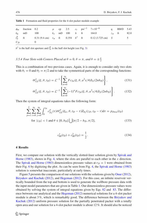
Table 1 Formation and fluid properties for the 4-slot packer module example

φm fraction 0.2 μ cp 2.5 ct psi−1 7×10−6 q RB/D 5.43

kh mD 100 kv mD 100 h ft 164.0 zw ft 82.0

l§w ft 0.31 (9.4 cm) rw ft 0.354 b† ft 0.12 (3.725 cm) S 5

CD 0

b† is the half slot aperture and l§w is the half slot height (see Fig. 3)

3.5.4 Four Slots with Centers Placed at θ = 0, θ = π , and θ = ±π2

This is a combination of two previous cases. Again, it is enough to consider only two slotswith θ1 = 0 and θ2 = π/2 and to take the symmetrical parts of the corresponding functions:

Θ1s2i (ξ, θ, tD) = L−1

{ ∞∑

n=0

Fc2n(ξ, θ, a2s/4)J2i (2nbD)

}

, (131)

Θ2s2i (ξ, θ, tD) = L−1

{ ∞∑

n=0

(−1)n Fc2n(ξ, θ, a2s/4)J2i (2nbD)

}

. (132)

Then the system of integral equations takes the following form:

2∑

p=1

∞∑

i=0

∞∑

j=0

∫ tD

0cp

2i j (τ )Θps2i (ξw, θ, tD − τ)Zhj (zD, tD − τ)dτ = pDwu(tD)

for |zD| < 1 and θ ∈ [0, bD]⋃

[π/2 − bD, π/2], (133)

c100(tD)+ c2

00(tD) = 1

2. (134)

4 Results

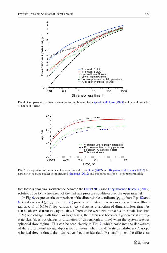
First, we compare our solution with the vertically slotted-liner solution given by Spivak andHorne (1983), shown in Fig. 4, where the slots are parallel to each other in the x direction.The Spivak and Horne (1983) dimensionless pressure values at rD = 1 were obtained fromtheir Fig. 6 by digitizing the plot. As can be seen from Fig. 4, the Spivak and Horne (1983)solution is somewhat inaccurate, particularly at early times.

Figure 5 presents the comparison of our solutions with the solutions given by Onur (2012),Biryukov and Kuchuk (2012), and Hegeman (2012). For this case, an infinite reservoir ver-tically bounded from the top and bottom is used to generate the wellbore pressure data withthe input model parameters that are given in Table 1. Our dimensionless pressure values wereobtained by solving the system of integral equations given by Eqs. 82 and 83. The differ-ence between our analytical and the Hegeman (2012) numerical solutions for a 4-slot packermodule is about 3 %, which is remarkably good. The difference between the Biryukov andKuchuk (2012) uniform pressure solution for the partially penetrated packer with a totallyopen area and our solution for a 4-slot packer module is about 12 %. It should also be noticed

123


0.1

2

3

4567

1

2

3

456

Dim

ensi

onle

ss p

ress

ure,

pD

0.01 0.1 1 10 100 1000

Dimensionless time, tD

This work: 3 slots This work: 6 slots Spivak-Horne: 3 slots Spivak-Horne: 6 slots Uniform-pressure partially penetrated Fully open cylindrical-source

Fig. 4 Comparison of dimensionless pressures obtained from Spivak and Horne (1983) and our solutions for3- and 6-slot cases

60

50

40

30

p, p

si

0.0001 0.001 0.01 0.1 1 10

Time, hr

Wilkinson-Onur partilaly penetrated Biryukov-Kuchuk partilaly penetrated Hegeman (numerical): 4 slots This work: 4 slots

Fig. 5 Comparison of pressures changes obtained from Onur (2012) and Biryukov and Kuchuk (2012) forpartially penetrated packer solutions, and Hegeman (2012) and our solutions for a 4-slot packer module

that there is about a 4 % difference between the Onur (2012) and Biryukov and Kuchuk (2012)solutions due to the treatment of the uniform pressure condition over the open interval.

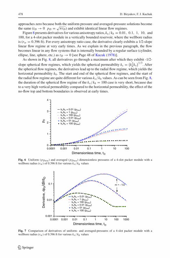
In Fig. 6, we present the comparison of the dimensionless uniform (pDwu from Eqs. 82 and83) and averaged (pDwa from Eq. 51) pressures of a 4-slot packer module with a wellboreradius (rw) of 0.396 ft for various kv/kh values as a function of dimensionless time. Ascan be observed from this figure, the differences between two pressures are small (less than12 %) and change with time. For large times, the difference becomes a geometrical steady-state skin (does not change as a function of dimensionless time) when the system reachesspherical flow regime. This can be seen clearly in Fig. 7, which compares the derivativesof the uniform-and averaged-pressure solutions, when the derivatives exhibit a -1/2-slopespherical flow regimes, their derivatives become identical. For small times, the difference

123


approaches zero because both the uniform pressure and averaged-pressure solutions becomethe same (tD → 0 pD = √

π tD) and exhibit identical linear flow regimes.Figure 8 presents derivatives for various anisotropy ratios, kv/kh = 0.01, 0.1, 1, 10, and

100, for a 4-slot packer module in a vertically bounded reservoir, where the wellbore radiusis (rw = 0.396 ft). For every anisotropy ratio case, the derivative clearly exhibits a 1/2-slopelinear flow regime at very early times. As we explain in the previous paragraph, the flowbecomes linear in any flow systems that is internally bounded by a regular surface (cylinder,ellipse, line, sphere, etc.) as tD → 0 [see Page 48 of Kucuk (1978)].

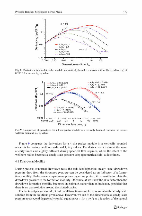
As shown in Fig. 8, all derivatives go through a maximum after which they exhibit -1/2-

slope spherical flow regimes, which yields the spherical permeability ks = (k2hkv)1/3

. Afterthe spherical flow regimes, the derivatives lead up to the radial flow regime, which yields thehorizontal permeability kh . The start and end of the spherical flow regimes, and the start ofthe radial flow regime are quite different for various kv/kh values. As can be seen from Fig. 8,the duration of the spherical flow regime of the kv/kh = 100 case is very short, because dueto a very high vertical permeability compared to the horizontal permeability, the effect of theno-flow top and bottom boundaries is observed at early times.

4

3

2

1

0

p D

0.0001 0.001 0.01 0.1 1 10 100

Dimensionless time, t D

kv/kh = 0.01 (pDwu)kv/kh = 1 (pDwu)kv/kh = 100 (pDwu)kv/kh = 0.01 (pDwa)kv/kh = 01 (pDwa)kv/kh = 100 (pDwa)

Fig. 6 Uniform (pDwu ) and averaged (pDwa ) dimensionless pressures of a 4-slot packer module with awellbore radius (rw) of 0.396 ft for various kv/kh values

0.001

0.01

0.1

Der

ivat

ive,

dp D

/dln

t D

0.0001 0.001 0.01 0.1 1 10 100 1000


m = - 1/2

kv/kh = 0.01 (pDwu)kv/kh = 1 (pDwu)kv/kh = 100 (pDwu)kv/kh = 0.01 (pDwa)kv/kh = 01 (pDwa)kv/kh = 100 (pDwa)

Fig. 7 Comparison of derivatives of uniform- and averaged-pressures of a 4-slot packer module with awellbore radius (rw) of 0.396 ft for various kv/kh values

123


0.001

0.01

0.1

1

Der

ivat

ive,

dp D

/dln

t D

0.0001 0.001 0.01 0.1 1 10 100


m = 1/2

m = - 1/2

kv /kh = 0.01 kv /kh = 0.1 kv /kh = 1 kv /kh = 10 kv /kh = 100

Fig. 8 Derivatives for a 4-slot packer module in a vertically bounded reservoir with wellbore radius (rw) of0.396 ft for various kv/kh values

0.001

0.01

0.1

1

Der

ivat

ive,

dp D

/dln

t D

0.0001 0.001 0.01 0.1 1 10 100 1000


m = 1/2

m = - 1/2

m = - 1/2

m = - 1/2

kv/kh = 0.01 (0.291) kv/kh = 1 (0.291) kv/kh = 100 (0.291)

kv/kh = 0.01( 0.354) kv/kh = 1 (0.354) kv/kh = 100 (0.354)

kv/kh = 0.01 (0.396) kv/kh = 1 (0.396) kv/kh = 100 (0.396)

Fig. 9 Comparison of derivatives for a 4-slot packer module in a vertically bounded reservoir for variouswellbore radii and kv/kh values

Figure 9 compares the derivatives for a 4-slot packer module in a vertically boundedreservoir for various wellbore radii and kv/kh values. The derivatives are almost the sameat early times and slightly different during spherical flow regimes, where the effect of thewellbore radius becomes a steady-state pressure drop (geometrical skin) at late times.

4.1 Drawdown Mobility

During pretests or normal drawdown tests, the stabilized (spherical steady-state) drawdownpressure drop from the formation pressure can be considered as an indicator of a forma-tion mobility. Under some simple assumptions regarding pretest, it is possible to relate thedrawdown pressure to the formation mobility. Of course, if we know the skin factor then thedrawdown formation mobility becomes an estimate, rather than an indicator, provided thatthere is no gas evolution around the slotted-packer.

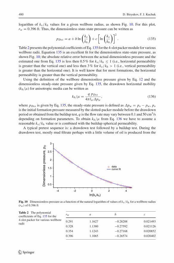
For the 4-slot packer module, it is difficult to obtain a simple expression for the steady-statesolution from the solutions given above. However, we can fit the dimensionless steady-statepressure to a second degree polynomial equation (a + bx + cx2) as a function of the natural

123


logarithm of kv/kh values for a given wellbore radius, as shown Fig. 10. For this plot,rw = 0.396 ft. Thus, the dimensionless state-state pressure can be written as

pDss = a + b ln

(kvkh

)+ c

[ln

(kvkh

)]2

. (135)

Table 2 presents the polynomial coefficients of Eq. 135 for the 4-slot packer module for variouswellbore radii. Equation 135 is an excellent fit for the dimensionless state-state pressure, asshown Fig. 10; the absolute relative error between the actual dimensionless pressure and theestimated one from Eq. 135 is less then 0.5 % for kv/kh ≤ 1 (i.e., horizontal permeabilityis greater than the vertical one) and less then 3 % for kv/kh > 1 (i.e., vertical permeabilityis greater than the horizontal one). It is well know that for most formations, the horizontalpermeability is greater than the vertical permeability.

Using the definition of the wellbore dimensionless pressure given by Eq. 12 and thedimensionless steady-state pressure given by Eq. 135, the drawdown horizontal mobility(kh/μ) for anisotropic media can be written as

kh/μ = q pDss

4πlwΔpw, (136)

where pDss is given by Eq. 135, the steady-state pressure is defined as Δpw = po − pw , po

is the initial formation pressure measured by the slotted-packer module before the drawdownperiod or obtained from the buildup test, q is the flow rate may vary between 0.1 and 50 cm3/sdepending on formation parameters. To obtain kh/μ from Eq. 136 we have to assume areasonable kv/kh value or is combined with the buildup spherical permeability.

A typical pretest sequence is: a drawdown test followed by a buildup test. During thedrawdown test, mostly mud filtrate perhaps with a little volume of oil is produced from the

3

2.5

2

1.5

1

0.5

Dim

ensi

onle

ss p

ress

ure,

pD

420-2-4

ln(kv/kh)

data

Fig. 10 Dimensionless pressure as a function of the natural logarithm of values of kv/kh for a wellbore radius(rw) of 0.396 ft

Table 2 The polynomialcoefficients of Eq. 135 for the4-slot packer for various wellboreradii

rw a b c

0.291 1.1627 −0.28288 0.021493

0.328 1.1380 −0.27592 0.021126

0.354 1.1243 −0.27168 0.020852

0.396 1.1065 −0.26574 0.020402

123


4-slot packer module, and the produced volume is normally small. The pressure at the packerinterval reaches quickly a spherical steady-state condition, unless the permeability formationis very low.

5 Conclusions

In this work, we have considered mixed boundary value problems for pressure transientdiffusion in porous media arising in connection with the pressure transient behavior of for-mation tests conducted with the Wireline Formation Testing (WFT) vertically slotted-packerconfiguration in a vertical well. The solutions in this paper are essentially based on the ideaof introducing an unknown flux density function on the open section (slot) of the wellbore,and its expansion in terms of singular basis functions. These functions reduce the mixedboundary value problem to a system of linear algebraic equations of modest size, which iseasy to solve numerically. Such solutions also prove to be accurate, numerically stable. Itis shown that the existing analytical solution is somewhat inaccurate. The anisotropy ratio(kv/kh) significantly affects the pressure transient behavior of the slot packer module. Thewellbore radius also affects the pressure transient behavior the system. Finally, we have givena formula to obtain the drawdown horizontal mobility (kh/μ) for anisotropic media.

Acknowledgments The authors are grateful to Schlumberger for permission to publish this paper.

Open Access This article is distributed under the terms of the Creative Commons Attribution License whichpermits any use, distribution, and reproduction in any medium, provided the original author(s) and the sourceare credited.

Appendix 1

In this section we present an efficient way to evaluate the functions Z j , Z jh andΘ2i . Z j canbe easily evaluated by passing into Laplace domain

Z j (zD, u, tD) = 2√π tDν

∫ π

0e−(zD−cos η)2/(4ν2tD) cos( jη)dη

= 2√π tDν

L−1(∫ π

0

cos( jη)dη

s + (zD − cos η)2,

1

4ν2tD

)

= 2√π tDν

L−1(

1

2i√

s

∫ π

0

cos( jη)dη

(zD + i√

s − cos η)

− cos( jη)dη

(zD − i√

s − cos η),

1

4ν2tD

)

= 2√π tDν

I mL−1(

1√s

∫ π

0

cos( jη)dη

(zD + i√

s − cos η),

1

4ν2tD

). (137)

The last integral can be evaluated using the following result from Prudnikov et al. (1981)

∫ π

0

cos( jη)dη

a + cos η=

⎧⎪⎨

⎪⎩

π√1−a2

(√1 − a2 − a

) jif |a| ≤ 1,

π√a2−1

(√a2 − 1 − a

) jif |a| > 1.

(138)

123


In the same way, the Laplace transform is useful when evaluating Z jh . The Laplace transformof Zh can be written as follows (see Erdelyi (1954))

L [Zh(zD, u, tD)] =∞∑

l=0

(−1)l e−(zD−u+2zDw+2lh D)√

s/ν2

√sν

+∞∑

l=1

[e−(2lhD+u−zD)

√s/ν2

√sν

+e−(zD−u+2lh D)√

s/ν2

√sν

+ (−1)l e−(2lhD−zD+u−2zDw)√

s/ν2

√sν

]

. (139)

The infinite summation can now easily be performed, we then obtain

L [Zh(zD, u, tD)] = e−(zD−u+2zDw)√

s/ν2

√sν(1 + e−2h D

√s/ν2

)+ e−(2hD+u−zD)

√s/ν2

√sν(1 − e−2h D

√s/ν2

)

+ e−(zD−u+2h D)√

s/ν2

√sν(1 − e−2h D

√s/ν2

)+ e−(2hD−zD+u−2zDw)

√s/ν2

√sν(1 + e−2h D

√s/ν2

), (140)

and consequently we get the following expression for the Laplace transform of Zhj

L[Zhj (zD, tD)

] = πe−(zD+2zDw)√

s/ν2(−1) j I j (

√s/ν2)

2√

2s(

1 − e−2hD

√s/ν2) +

πe−(2hD−zD)√

s/ν2(−1) j I j

(√s/ν2

)

2√

2s(

1 − e−2hD

√s/ν2)

+πe−(zD+2hD)

√s/ν2

I j

(√s/ν2

)

2√

2s(

1−e−2hD

√s/ν2) +

πe−(2hD−zD−2zDw)√

s/ν2I j

(√s/ν2

)

2√

2s(

1−e−2hD

√s/ν2) ,

(141)

where I j is the Modified Bessel function of the First kind.Now let us consider the function Θ2i (1, θ, tD). It can be seen that the series terms in

the Laplace domain in Eq. 34 are slowly convergent for rD = 1, but from Abramowitz andStegun (1972) we can find that

2Kn(√

s)

Kn−1(√

s)+ Kn+1(√

s)= −Kn(

√s)

K′n(

√s)

∼√

s√s + n2

(142)

for large n. Thus, we can rewrite Eq. 34 for rD = 1 as

Θ2i (1, θ, tD) = L−1

{1√s

∑

n=0

(1 − δ0n

2

)[2Kn(

√s)J2i (nbD) cos(nθ)

Kn+1(√

s)+ Kn−1(√

s)−

√s cos nθ√s + n2

]}

+ 1√π tD

∞∑

n=−∞e−n2tD J2i (nbD) cos(nθ). (143)

Now the first sum converges very fast (about 50 terms is enough to obtain 4-5 digits precision),while the second has a very high convergence rate for tD ≥ 1, due to the presence of theexponential term. The convergence rate, however, slows down rapidly for tD < 1, we,

123


therefore, propose to rewrite it in the following form:

∞∑

n=−∞

e−n2tD

√π tD

J2i (nbD) cos(nθ)

= (−1)i∫ π

0

∞∑

n=−∞

e−n2tD

π√π tD

cos(n[bD cosα + θ ]) cos(2iα)dα

= (−1)i√π tD

∞∑

n=−∞

∫ π

0e− (2πn/bD+θ/bD+cosα)2

4tD/b2D cos(2iα)dα. (144)

Note that here we used the Poisson summation formula. The last integral and summation canbe easily evaluated exactly by the same way as we described for Z j and Zhj above. A similartechnique without any significant changes can be also applied to evaluation of the functionΘN02i . It can also be shown that for large n

Fcn

(ξw, θ,

a2s

4

)→

2√

2Kn

(√sa2

2 sinh 2ξw

)cos nθ

√sa2 sinh 2ξw

[Kn−1

(√sa2

2 sinh 2ξw

)+ Kn+1

(√sa2

2 sinh 2ξw

)]

→ cos nθ√

sa2

2 sinh 2ξw + n2, (145)

and

Fsn

(ξw, θ,

a2s

4

)→

2√

2Kn

(√sa2

2 sinh 2ξw

)sin nθ

√sa2 sinh 2ξw

[Kn−1

(√sa2

2 sinh 2ξw

)+ Kn+1

(√sa2

2 sinh 2ξw

)]

→ sin nθ√

sa2

2 sinh 2ξw + n2. (146)

Thus, the series in Eqs. 115–116 can be rewritten as

Θp2i (ξ, θ, tD) = L−1

{∑

n=0

[Fcn

(ξ, θ,

a2s

4

)cos(nθp)+ Fsn

(ξ, θ,

a2s

4

)sin(nθp)

−(

1 − δ0n

2

)cos[n(θ − θp)]√sa2

2 sinh 2ξw + n2

]× J2i (nbD)

}

+√

2√

a2π sinh 2ξwtD

∞∑

n=−∞e− 2n2 tD

a2 sinh 2ξw J2i (nbD) cos[n(θ − θp)], (147)

Θp2i+1(ξ, θ, tD) = L−1

{∑

n=1

[Fsn

(ξ, θ,

a2s

4

)cos(nθp)− Fcn

(ξ, θ,

a2s

4

)sin(nθp)

− sin[n(θ − θp)]√sa2

2 sinh 2ξw + n2

]× J2i+1(nbD)

}

123


+√

2√

a2π sinh 2ξwtD

∞∑

n=−∞e− 2n2 tD

a2 sinh 2ξw J2i+1(nbD) sin[n(θ − θp)].

(148)

The last series in Eq. 147 has the same form as in the horizontally isotropic case, while theone in Eq. 148 can be rewritten as

√2

√a2π sinh 2ξwtD

∞∑

n=−∞e− 2n2 tD

a2 sinh 2ξw J2i+1(nbD) sin[n(θ − θp)]

= (−1)i∫ π

0

∞∑

n=−∞

√2e

− 2n2 tDa2 sinh 2ξw

π√

a2π sinh 2ξwtD

cos(n[bD cosα + θ − θp]) cos[(2i + 1)α]dα

= (−1)i√π tD

∞∑

n=−∞

∫ π

0e− (2πn/bD+[θ−θp ]/bD+cosα)2

4tD/(a2b2

D cosh ξw sinh ξw) cos[(2i + 1)α]dα, (149)

which can be summed up in the same way as we proposed for Z j and Zhj . The last point onwhich we want to focus is the computation of integrals in Eq. 40. On every subinterval [t1, t2]the functions Θ(p)

i (1, θ, tD), Z j (zD, tD) and Zhj (zD, tD) can be approximated as follows

Θ(p)i (1, θ, tD) = Ai (θ)

t1/2 + B j (θ)

t [i/2]+1D

, (150)

Z j (zD, tD) = C j (zD)+ D j (zD)

t [ j/2]+1/2D

, (151)

Zhj (zD, tD) =[

E j (zD)

t1/2D

+ Fj (zD)

t [ j/2]D

]

e− min(2zDw+zD−1,2h D−2zDw−1)2

4ν2 tD . (152)

We suggest computing the coefficients by a simple 2-point interpolation. Now the integralgiven in Eq. 40 can be written as

∫ a2

a1

τ−αe−β/τdτ =∫ 1/a1

1/a2

uα−2e−βudu = e−β/a2

aα−12

∫ a2/a1

1vα−2e

− βa2(v−1)

dv. (153)

Although the last integral can be expressed in terms of incomplete gamma functions, onecan see that for a 4-step time scheme we proposed above, a2/a1 can take only the followingvalues: 2, 1.5, and 4/3. Thus, this integral is a function of only one variable β

a2(while a2/a1

and α constitute only a finite set of parameters) and, therefore, can easily be approximatedin a wide range using, for example, cubic splines for moderate values of β

a2and some simple

asymptotic approximations for very small and very big values.

References

Abramowitz, M., Stegun, I.: Handbook of Mathematical Functions. Dover, New York (1972)Al-Otaibi, S., Bradford, C., Zeybek, M., Corre, P.-Y., Slapal, M., Ayan, C., Kristensen, M.: Oil–water delin-

eation with a new formation tester module. In: Paper SPE 159641, SPE Annual Technical Conferenceand Exhibition, San Antonio, Texas, USA, 8–10 October (2012)

Besson, J.: Performance of slanted and horizontal wells on an anisotropic medium. In: Paper SPE-20965-MS,European Petroleum Conference, The Hague, the Netherlands, 21–24 October (1990)

123


Biryukov, D., Kuchuk, F.J.: Pressure transient solutions to mixed boundary value problems for partially openwellbore geometries in porous media. J. Pet. Sci. Eng. 96–97, 162–175 (2012)

Brons, F., Marting, V.E.: The effect of restricted fluid entry on well productivity. J. Pet. Technol. 13(2), 172–174(1961)

Erdelyi, A.E.: Tables of Integral Transforms, vol. 1. McGraw-Hill (Bateman project), New York (1954)Flores de Dios, T., Aguilar, M.G., Herrera, R.P., Garcia, G., Peyret, E., Ramirez, E., Arias, A., Corre, P.-Y.,

Slapal, M., Ayan, C.: New wireline formation tester development makes sampling and pressure testingpossible in extra-heavy oils in Mexico. In: Paper SPE 159868, SPE Annual Technical Conference andExhibition, San Antonio, Texas, USA, 8–10 October (2012)

Goode, P., Wilkinson, D.: Inflow performance of partially open horizontal wells. J. Pet. Technol. 43 (1991)Gringarten, A.C., Ramey, H.J.J.: An approximate infinite conductivity solution for a partially penetrating

line-source well. Trans. AIME 259, 140–148 (1975)Hantush, M.S.: Non-steady flow to a well partially penetrating an infinite leaky aquifer. Proc. lraqi Sci. Soc.

1, 10–19 (1957)Hegeman, P.: Sotted-wellbore numerical solution. Personal communication. (2012)Kuchuk, F.: Pressure behavior of MDT packer module and DST in crossflow-multilayer reservoirs. J. Pet. Sci.

Eng. 11(2), 123–135 (1994)Kuchuk, F.: Interval pressure transient testing with MDT packer-probe module in horizontal wells. SPE

Reservoir Eval. Eng. 1(6), 509–518 (1998)Kuchuk, F., Onur, M., Hollaender, F.: Pressure Transient Formation and Well Testing: Convolution, Deconvo-

lution and Nonlinear Estimation. Elsevier, New York (2010)Kuchuk, F.J., Onur, M.: Estimating permeability distribution from 3D interval pressure transient tests. J. Pet.

Sci. Eng. 39, 5–27 (2003)Kuchuk, F.J., Wilkinson, D.: Pressure behavior of commingled reservoirs. SPE Form. Eval. 6(1), 111–120

(1991)Kucuk, F.: Transient flow in elliptical systems. PhD thesis, Stanford University, Stanford, CA (1978)Larsen, L.: The pressure-transient behavior of vertical wells with multiple flow entries. Paper SPE 26480, SPE

Annual Technical Conference and Exhibition, 3–6 October, Houston, Texas, (1993)Muskat, M.: The Flow of Homogeneous Fluids Through Porous Media. J. W. Edwards Inc., Ann Arbor (1937)Nisle, R.G.: The effect of partial penetration on pressure build-up in oil wells. Trans. AIME 213, 85–90 (1958)Odeh, A.S.: Steady-state flow capacity of wells with limited entry to flow. SPE J. 8(1), 43–51 (1968)Onur, M.: Partially pettrated well model. Personal communication (2012)Onur, M., Hegeman, P., Gok, I., Kuchuk, F.: A novel analysis procedure for estimating thickness-independent

horizontal and vertical permeabilities from pressure data at an observation probe acquired by packer-probe wireline formation testers. SPE Reservoir Eval. Eng. 14(4), 457–472 (2011)

Onur, M., Hegeman, P., Kuchuk, F.: Pressure-transient analysis of dual packer-probe wireline formation testersin slanted wells. In: Paper SPE 90250, SPE Annual Technical Conference and Exhibition, Houston, Texas,26–29 September (2004a)

Onur, M., Hegeman, P., Kuchuk, F.J.: Pressure-pressure convolution analysis of multiprobe and packer-probewireline formation tester data. SPE Reservoir Eval. Eng. 7(5), 351–364 (2004b)

Onur, M., Kuchuk, F. J.: Integrated nonlinear regression analysis of multiprobe wireline formation testerpacker and probe pressures and flow rate measurements. In: Paper SPE 56616, SPE Annual TechnicalConference and Exhibition, Houston, 3–6 October (1999)

Ozkan, E., Raghavan, R.: New solutions for well-test-analysis problems: Part 1—Analytical considerations.SPE Form. Eval. 6(3), 359–368 (1991)

Papatzacos, P.: Approximate partial-penetration pseudoskin for infinite-conductivity wells. SPE ReservoirEng. 2(2), 227–234 (1987a)

Papatzacos, P.: Exact solutions for infinite-conductivity wells. SPE Reservoir Eng. 2(2), 217–226 (1987b)Pop, J., Badry, R., Morris, C., Wilkinson, D., Tottrup, P., Jonas, J.: Vertical interference testing with a wireline-

conveyed straddle-packer tool. In: Paper SPE 26481, SPE Annual Technical Conference and Exhibition,Houston, Texas, 3–6 October (1993)

Prudnikov, A., Brychkov, Y., Marichev, O.I.: Integrali i ryadi. Nauka, Moscow, Elementarnie funkcii (inRussian) (1981)

Spivak, D., Horne, R.N.: Unsteady-state pressure response due to production with a slotted liner completion.J. Pet. Technol. 35(7), 1366–1372 (1983)

Streltsova-Adams, T.D.: Pressure drawdown in a well with limited flow entry. J. Pet. Technol. 31(11), 1469–1476 (1979)

Tang, Y., Ozkan, E., Kelkar, M., Sarica, C., Yildiz, T.: Performance of horizontal wells completed with slottedliners and perforations. In: Paper SPE 65516, SPE/CIM International Conference on Horizontal WellTechnology, Calgary. Alberta, Canada, 6–8 (2000)

123


Wilkinson, D., Hammond, P.: A perturbation method for mixed boundary-value problems in pressure transienttesting. Trans. Porous Media 5, 609–636 (1990)

Schlumberger: Wireline-Schlumberger: Saturn 3D radial probe brochure (2012)Yildiz, T.: Productivity of horizontal wells completed with screens. In: Paper SPE 76712, SPE Western

Regional/AAPG Pacific Section Joint Meeting, Anchorage, Alaska, 20–22 May (2002a)Yildiz, T.: Productivity of selectively perforated vertical wells. SPE J. 7(2), 158–169 (2002b)Yildiz, T.: Productivity of horizontal wells completed with screens. Reservoir Eval. Eng. 7(5), 342–350 (2004)Yildiz, T.: Assessment of total skin factor in perforated wells. Reservoir Eval. Eng. 9(1), 61–76 (2006a)Yildiz, T.: Productivity of selectively perforated horizontal wells. SPE Prod. Oper. 21(1), 75–80 (2006b)Yildiz, T., Bassiouni, Z.: Transient pressure analysis in partially-penetrating wells. In: Paper SPE-21551-MS,

CIM/SPE International Technical Meeting, Calgary, Alberta, Canada, 10–13 June (1990)Yildiz, T., Cinar, Y.: Inflow performance and transient pressure behavior of selectively completed vertical

wells. SPE Reservoir Eval. Eng. 1(5), 467–475 (1998)Zeybek, M., Kuchuk, F., Hafez, H.: Fault and fracture characterization using 3D interval pressure transient

tests. In: Paper SPE 78506, Abu Dhabi International Petroleum Exhibition and Conference, Abu Dhabi,UAE, 13–16 October (2002)

Zimmerman, T., MacInnis, J., Hoppe, J., Pop, J., Long, T.: Application of emerging wireline formation testingtechnologies. In: OSEA 90105, 8th Offshore South East Asia Conference, Singapore, 4–7 December(1990)

123