ERJ Engineering Research Journal
Faculty of Engineering Menoufia University
Engineering Research Journal, Vol. 42, No. 2, April 2019, PP: 99-114
© Faculty of Engineering, Menoufia University, Egypt
99
PREDICTION OF TWO-PHASE PRESSURE DROP USING
ARTIFICIAL NEURAL NETWORK
M.A. El-Kadi
1, M.A. Husien
1, S.M. El-Behery
1 and H. Farouk
2
1 Mechanical Power Engineering Dept., Faculty of Engineering, Menoufia University,
Shebin Elkom, Egypt. 2 MAGAPETCO - Magawish Petroleum Co., Cairo, Egypt
ABSTRACT: In the present paper an Artificial Neural Network (ANN) model is proposed to predict the two-phase pressure
drop in oil and gas field. In this model, the effect of number of hidden layers and number of neurons in each
layer is selected to generate independent results. In addition, the selected database contains 7581 data sets
selected from four different sources from which 1165 data sets are collected from the flowing wells of
Magapetco at East Esh Mallaha Marine (EEMM) field. The comparison between ANN predictions and other
popular models reveals that the ANN model can predict the pressure drop with fair accuracy. Furthermore, the
proposed model is used to predict the pressure distribution along the wall of flowing wells as well as the bottom
hole flowing pressure and good accuracy was obtained.
Keywords:- Neural network, pressure drop, two-phase, oil and gas.
1. NTRODUCTION The (ANN) was used since 1990s to do the
same function of empirical and mechanistic
correlations for predicting the flowing well bottom hole pressure with some known well parameters. In
1995 Ternyik et al. [1] explored application of a
new ANN model to predict the bottom hole flowing
pressure. They used the back propagation network
and trained it with Mukharjee and Brill [2]
experimental data. In 2002 another study done by
Shippen and Scott [3], they developed a three layer
back propagation ANN to predict the two-phase
holdup in a horizontal flow. They used 627 holdup
measurements for network training. Osman [4]
proposed a three layer BP network predict the
liquid holdup and flow regime in horizontal multi-
phase flow using 199 experimental data sets.
Osman et al. [5] introduced another
network to predict the flowing bottom-hole pressure
in vertical multi-phase flow. They compared their
network with the conventional empirical and mechanistic models showed that the ANN was the
best. Ozbayoglu and Ozbayoglu [6] presented
different types of ANN to predict the frictional
pressure loss and the flow regime of horizontal
multi-phase flow. Mohammadpoor et al. [7]
conducted a new ANN to predict the bottom-hole
flowing pressure in vertical multiphase oil well in
Iranian oil fields. He tested different layers neurons
of ANN and various training functions and used
the best of them which had the minimum error.
Ashena et al. [8] trained ANN with
varying the number of neurons to predict the
pressure drop in annular multi-phase flow based on
Iranian oil field data sets. Adebayo et al. [9]
performed a comparison between different training
functions, where, the “trainlm” function was
selected as the best function. They used a total of
795 data sets from well test data to predict the
bottom-hole pressure in vertical wells. Li et al. [10]
trained different neural network models corresponding to different flow regimes utilizing a
new model for bottom hole flowing pressure
prediction. Ebrahimi and Khamehchi [11] proposed
an ANN to compute the pressure drop in multi-
phase vertical oil well. A total number of 1740 data
collected from the Middle East region wells were
used to train and test the ANN.
All the previous ANN models achieved
higher accuracy when compared with conventional
pressure drop estimation correlations.
Noted that most of the previously
mentioned ANN models used the total pressure
drop in the used pipe or well bore as one segment
which may reduce the accuracy of the obtained
results for deviated wells. For this reason the
pipeline or well bore used in this study divided into
segments by the rule of traverse method as will be explained later.
2. MATHEMATICAL MODEL In the human brain, a typical neuron
collects signals from others through a host of fine
structures called dendrites. The neuron sends out
spikes of electrical activity through a long, thin
stand known as an axon, which splits into
thousands of branches. At the end of each branch, a
structure called a synapse converts the activity from
the axon into electrical effects that inhibit or excite
activity in the connected neurons. Neural Network
is an information processing model that is inspired
by the biological nervous systems, such as the
human brain’s information processing mechanism.
M.A. El-Kadi, M.A. Husien, S.M. El-Behery , H. Farouk “PREDICTION OF TWO-PHASE PRESSURE …”
Engineering Research Journal, Menoufiya University, Vol. 42, No. 2, April 2019 100
An ANN is configured for a specific application, such as pattern recognition or data
classification, through a learning process. The key
element of this model is the novel structure of the
information processing system. It is composed of a
large number of highly interconnected processing
elements (neurons) working in unison to solve
specific problems. ANNs, like people, learn by
example. A neuron performs two simple tasks
which are weighted summation of its input array
and the application of a sigmoid function (S-
shaped) to this summation to give an output which
can serve as input to other neurons.
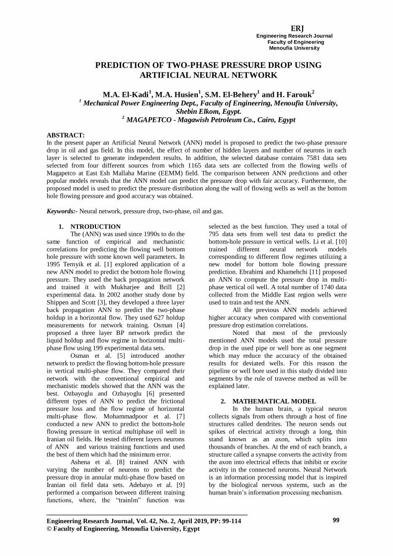
An ANN consists of an input layer, an
output layer, and one or more hidden layers. The
input layer contains an array of variables into which
the input data of the system is read from an external
source. Similarly, the predicted data or results, which can be multiple vectors, are written in the
output layer. Initially, the input layer receives the
input and passes it to the first hidden layer for
processing. The processed information from the
first hidden layer is then passed to the other hidden
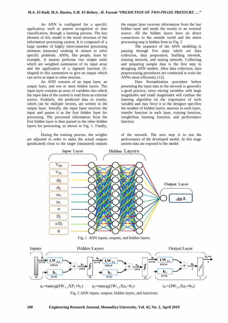
layers for processing, as shown in Fig. 1. Finally,
the output layer receives information from the last hidden layer and sends the results to an external
source. All the hidden layers have no direct
connections to the outside world and the entire
processing step is hidden from us Fig. 2
The sequence of the ANN modeling is
passing through five steps which are data
collection, data preparation, building network,
training network, and testing network. Collecting
and preparing sample data is the first step in
designing ANN models. After data collection, data
preprocessing procedures are conducted to train the
ANNs more efficiently [12].
Data Normalization procedure before
presenting the input data to the network is generally
a good practice, since mixing variables with large
magnitudes and small magnitudes will confuse the
learning algorithm on the importance of each variable and may force it to the designer specifies
the number of hidden layers, neurons in each layer,
transfer function in each layer, training function,
weight/bias learning function, and performance
function
.
During the training process, the weights
are adjusted in order to make the actual outputs
(predicated) close to the target (measured) outputs
of the network. The next step is to test the
performance of the developed model. At this stage
unseen data are exposed to the model.
Fig. 1 ANN inputs, outputs, and hidden layers.
Fig. 2 ANN inputs, outputs, hidden layers, and functions.
M.A. El-Kadi, M.A. Husien, S.M. El-Behery , H. Farouk “PREDICTION OF TWO-PHASE PRESSURE …”
Engineering Research Journal, Menoufiya University, Vol. 42, No. 2, April 2019 101
2.1. Data Collection A Total 7581 data sets are collected from four different independent sources. The distribution of these
data is given in table 1.
Table 1. The detailes of collected data distribution.
Data Source Stanford University
Data Bank [19]
Weihong
Meng [20]
Beggs and
Brill [21] EEMM Total
Number of Data sets 5658 176 582 1165 7581
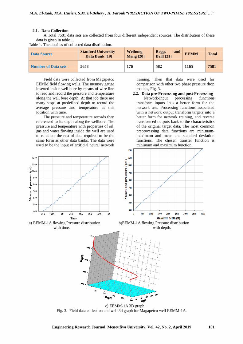
Field data were collected from Magapetco
EEMM field flowing wells. The memory gauge
inserted inside well bore by means of wire line
to read and record the pressure and temperature
along the well bore depth. At that job there are
many stops at predefined depth to record the
average pressure and temperature at this
location with time.
The pressure and temperature records then referenced to its depth along the wellbore. The
pressure and temperature with properties of oil,
gas and water flowing inside the well are used
to calculate the rest of data required to be the
same form as other data banks. The data were
used to be the input of artificial neural network
training. Then that data were used for
comparison with other two phase pressure drop
models, Fig. 3.
2.2. Data pre-Processing and post-Processing Network-input processing functions
transform inputs into a better form for the
network use. Processing functions associated
with a network output transform targets into a
better form for network training, and reverse transformed outputs back to the characteristics
of the original target data. The most common
preprocessing data functions are minimum-
maximum and mean and standard deviation
functions. The chosen transfer function is
minimum and maximum function.
a) EEMM-1A flowing Pressure distribution b)EEMM-1A flowing Pressure distribution
with time. with depth.
c) EEMM-1A 3D graph.
Fig. 3. Field data collection and well 3d graph for Magapetco well EEMM-1A.
M.A. El-Kadi, M.A. Husien, S.M. El-Behery , H. Farouk “PREDICTION OF TWO-PHASE PRESSURE …”
Engineering Research Journal, Menoufiya University, Vol. 42, No. 2, April 2019 102
2.3. Building Network In the current study, back propagation feed
forward network is used. The number of hidden
layers and the number of neurons in each layer are
very important parameters when building the
network. In the current study, comparisons are
carried out between the model accuracy using one,
two, and three hidden layers and number of neurons
in each layer from 10 to 70 neurons, as shown in
Fig. 4. From this figure it can be seen that the
model accuracy don’t changed greatly when the neurons in increased from 60 to 70 neurons.
Therefore, 70 neurons can be used for the network
with fair accuracy. The figure shows also that the
accuracy of two hidden layers is higher than that of
three hidden layers. Therefore, a two hidden layers
network is chosen in the current study.
For the training functions the default
function (trainlm) is used. trainlm is a network
training function that updates weight and bias
values according to Levenberg-Marquardt
optimization. trainlm is often the fastest back-
propagation algorithm in Matlap program toolbox,
and is highly recommended as a first-choice
supervised algorithm, although it does require more
memory than other algorithms. As the percentage of dividing the inputs to
training, validating, and testing tested for the
available divisions, the best was 70, 15, and 15 for
training, validating, and testing respectively. The
selected network is shown in Fig. 5.
Fig. 4 Effect of number of hidden layers and number of neurons on ANN accuracy.
Fig. 5. Final selected ANN.
2.4. Training Network There are two network training types
namely supervised and unsupervised training. In the
supervised training, the network feed by inputs and
corresponding targets to predict the outputs of these
inputs. Then, the target compared with the output
leading to modifying the weights for each layer to
reduce the error between output and target. While
in the unsupervised training, the weights and biases
are modified in response to network inputs only.
There are no target outputs available. Most of these
algorithms perform clustering operations. In the
current study the appropriate type of training is the supervised training type to predict the pressure drop
from the two-phase flow properties inputs.
This network uses the following procedure
to achieve target. First step is to enter the input
data, and calculate its corresponding output; this
step is named feed forward process. The next step is
to calculate the error between the targets and
outputs. If the sum-squared-error between outputs
and corresponding targets isn’t in the required
M.A. El-Kadi, M.A. Husien, S.M. El-Behery , H. Farouk “PREDICTION OF TWO-PHASE PRESSURE …”
Engineering Research Journal, Menoufiya University, Vol. 42, No. 2, April 2019 103
range, then the error must be minimized by
readjusting the weights beginning with the last
layer. The same process of calculating error is
repeated back-propagated for the previous layers till
reaching the input layer. This process named back-
propagation. For more details in back-propagation
process, after calculating the outputs resulted from
providing the network with inputs, the error
between each output and corresponding target is
determined as:
E= (Ti -Yi) (1) Where: Ti is the outputs, Yi is the target
Then, the weights and biases are re-
adjusted from network learning process as follows:
ΔWi= Wi+1-Wi (2)
Where: Wi+1 is the new adjusted weight,
Wi is the old (original) weight
wi = LR E Xi (3)
Where: LR is a small constant (Example
0.01) named learning rate.
Then, the new weights can be calculated
from Eq. (2). Propagate backward to the previous
layer by also calculating errors and readjusting its
weights. Doing the same for all layers until reaches
the first inputs layer by readjusting the weights.
Step by step the errors between outputs and targets
will be in the desired range. Then that will be the
required network.
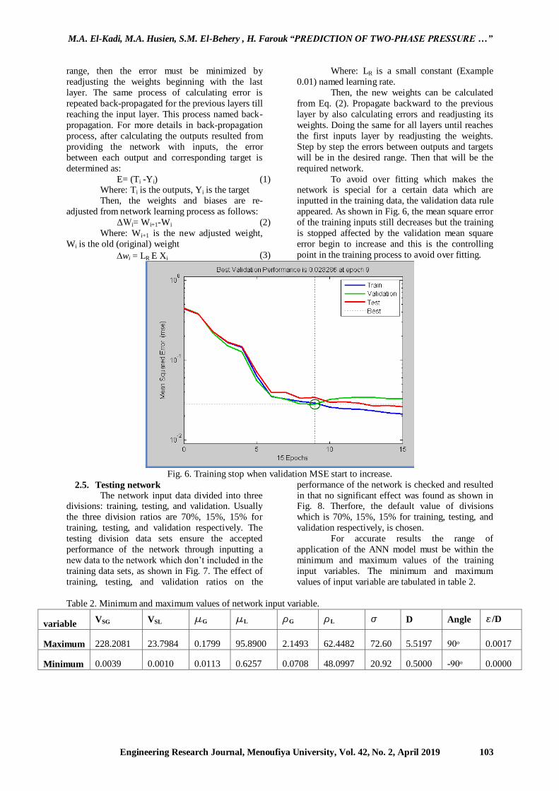
To avoid over fitting which makes the network is special for a certain data which are
inputted in the training data, the validation data rule
appeared. As shown in Fig. 6, the mean square error
of the training inputs still decreases but the training
is stopped affected by the validation mean square
error begin to increase and this is the controlling
point in the training process to avoid over fitting.
Fig. 6. Training stop when validation MSE start to increase.
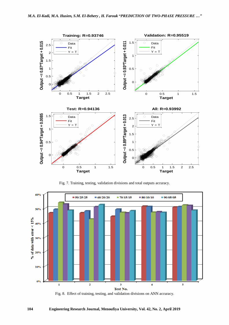
2.5. Testing network The network input data divided into three
divisions: training, testing, and validation. Usually
the three division ratios are 70%, 15%, 15% for
training, testing, and validation respectively. The
testing division data sets ensure the accepted
performance of the network through inputting a
new data to the network which don’t included in the
training data sets, as shown in Fig. 7. The effect of
training, testing, and validation ratios on the
performance of the network is checked and resulted
in that no significant effect was found as shown in Fig. 8. Therfore, the default value of divisions
which is 70%, 15%, 15% for training, testing, and
validation respectively, is chosen.
For accurate results the range of
application of the ANN model must be within the
minimum and maximum values of the training
input variables. The minimum and maximum
values of input variable are tabulated in table 2.
Table 2. Minimum and maximum values of network input variable.
variable VSG VSL mG mL rG rL s D Angle e/D
Maximum 228.2081 23.7984 0.1799 95.8900 2.1493 62.4482 72.60 5.5197 90ᵒ 0.0017
Minimum 0.0039 0.0010 0.0113 0.6257 0.0708 48.0997 20.92 0.5000 -90ᵒ 0.0000
M.A. El-Kadi, M.A. Husien, S.M. El-Behery , H. Farouk “PREDICTION OF TWO-PHASE PRESSURE …”
Engineering Research Journal, Menoufiya University, Vol. 42, No. 2, April 2019 104
Fig. 7. Training, testing, validation divisions and total outputs accuracy.
Fig. 8. Effect of training, testing, and validation divisions on ANN accuracy.
0 0.5 1 1.5 2 2.5
0
0.5
1
1.5
2
2.5
Target
Ou
tpu
t ~=
0.87
*Tar
get
+ 0
.015
Training: R=0.93746
Data
Fit
Y = T
0 0.5 1 1.5
0
0.5
1
1.5
Target
Ou
tpu
t ~=
0.93
*Tar
get
+ 0
.011
Validation: R=0.95519
Data
Fit
Y = T
0 0.5 1 1.5
0
0.5
1
1.5
Target
Ou
tpu
t ~=
0.94
*Tar
get
+ 0
.008
5
Test: R=0.94136
Data
Fit
Y = T
0 0.5 1 1.5 2 2.5
0
0.5
1
1.5
2
2.5
Target
Ou
tpu
t ~=
0.89
*Tar
get
+ 0
.013
All: R=0.93992
Data
Fit
Y = T
M.A. El-Kadi, M.A. Husien, S.M. El-Behery , H. Farouk “PREDICTION OF TWO-PHASE PRESSURE …”
Engineering Research Journal, Menoufiya University, Vol. 42, No. 2, April 2019 105
3. RESULTS AND DISCUSSION Six models of two-phase flow pressure
drop models were applied on the collected data to
select the most accurate model. The six models are:
1. Homogenous model [13] 2. Gray model [14] 3.
Beggs and Brill model [15] 4. Duns and Ros model
[16] 5. Mukherjee and Brill model [17] 6. Petalas
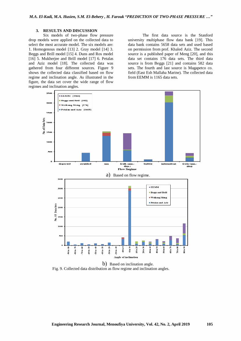
and Aziz model [18]. The collected data was
gathered from four different sources. Figure 9
shows the collected data classified based on flow
regime and inclination angle. As illustrated in the figure, the data set cover the wide range of flow
regimes and inclination angles.
The first data source is the Stanford
university multiphase flow data bank [19]. This
data bank contains 5658 data sets and used based
on permission from prof. Khaled Aziz. The second
source is a published paper of Meng [20], and this
data set contains 176 data sets. The third data
source is from Beggs [21] and contains 582 data
sets. The fourth and last source is Magapetco co.
field (East Esh Mallaha Marine). The collected data
from EEMM is 1165 data sets.
a) Based on flow regime.
b) Based on inclination angle. Fig. 9. Collected data distribution as flow regime and inclination angles.
M.A. El-Kadi, M.A. Husien, S.M. El-Behery , H. Farouk “PREDICTION OF TWO-PHASE PRESSURE …”
Engineering Research Journal, Menoufiya University, Vol. 42, No. 2, April 2019 106
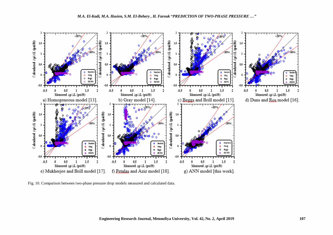
3.1. Comparison between Pressure Drop Models The accuracy of the tested models is
presented in Fig. 10. The figure shows a direct
comparison between measured and predicted
pressure drop data. It can be seen from this figure
that the ANN model gives the most accurate results.
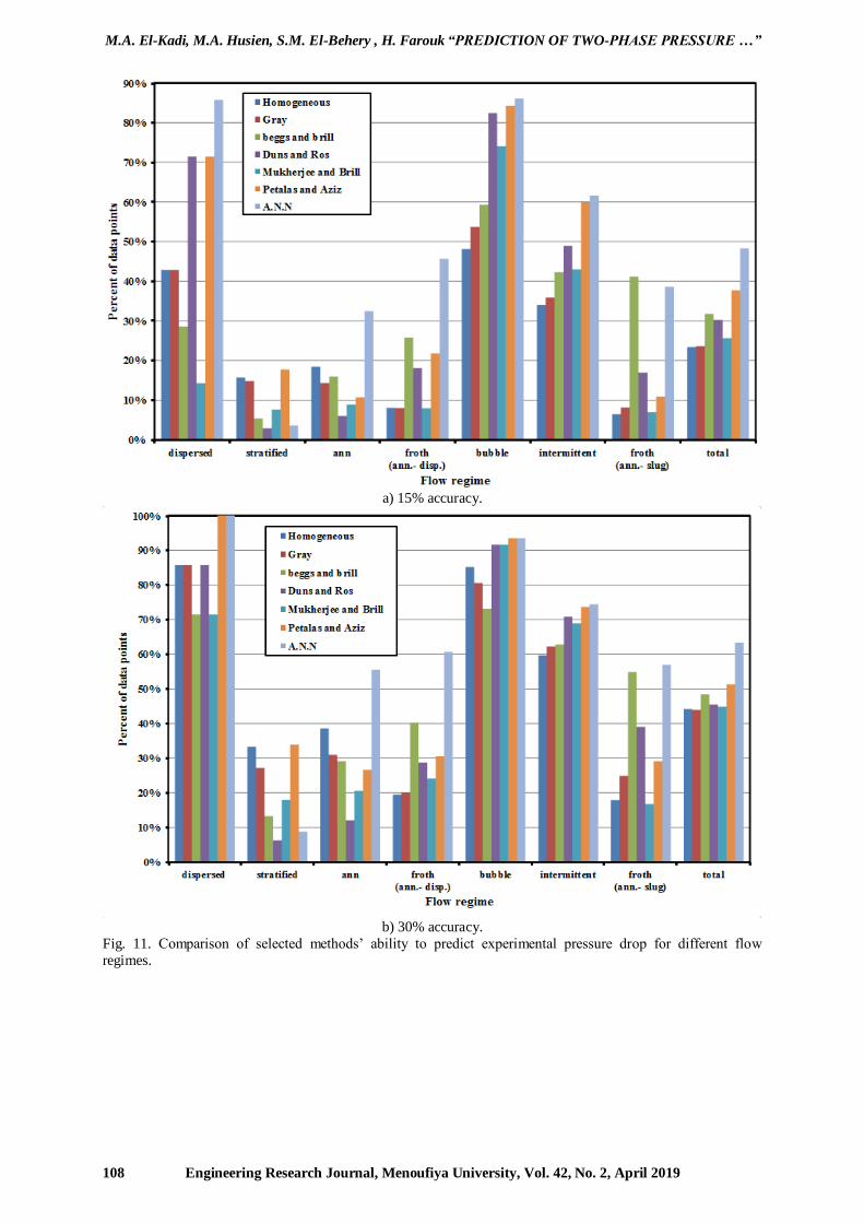
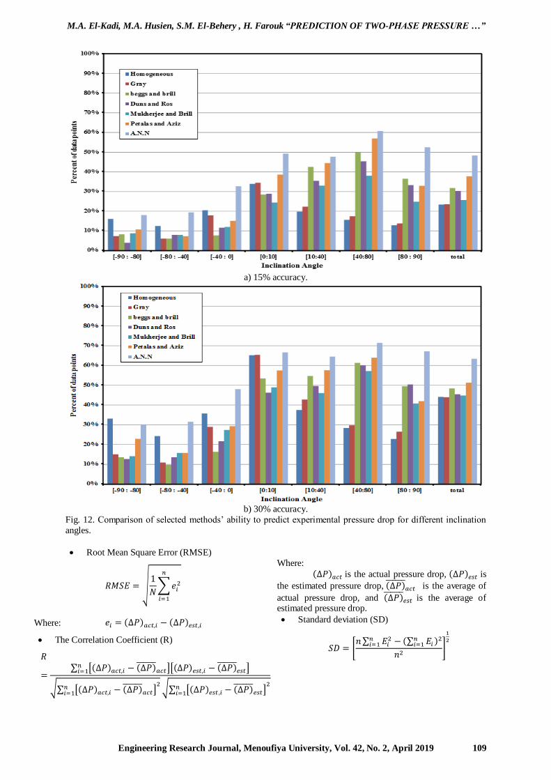
To quantify the accuracy of the tested
models, the ability of these models to predict the
pressure drop, data with 15% and 30% accuracy is
presented in Fig. 11 for different flow regimes and
in Fig. 12 for different inclination angles. It can be seen from this figures that the
ANN model predicts 48.27% of the data with an
accuracy of 15% and 63.39% of the data with an
accuracy of 30% for different flow regimes Fig. 11.
Despite this accuracy is low, it is quite acceptable
in multiphase where many parameters act. Figure
11 shows also that the highest accuracy is found for
dispersed and bubble flow regimes. These results
may be attributed to the homogeneity of these
regimes. In addition, the accuracy of all models was
low in downhill flows (negative inclination angles)
Fig. 12. This may be due to that the stratified flow
regime is the most dominated in this inclination
angles.
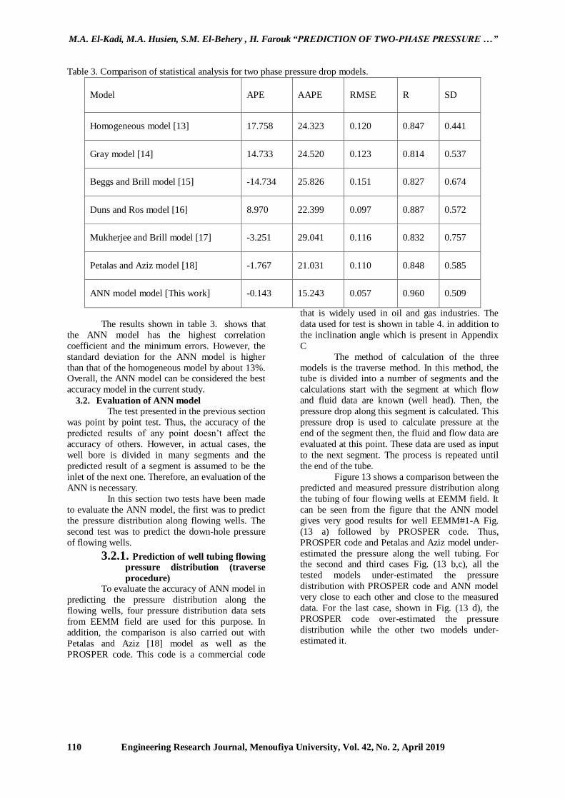
3.1.1. Statistical Analysis Statistical analysis was carried out for the
results of all two-phase pressure drop models and
this analysis is presented in the table 3. The
parameters of analysis presented in the next
equations.
Average Relative Percent Error (APE)
∑
(1)
Where:
[( ) ( )
( ) ]
Absolute Average Relative Percent Error
(AAPE)
∑| |
(2)
M.A. El-Kadi, M.A. Husien, S.M. El-Behery , H. Farouk “PREDICTION OF TWO-PHASE PRESSURE …”
Engineering Research Journal, Menoufiya University, Vol. 42, No. 2, April 2019 107
Fig. 10. Comparison between two-phase pressure drop models measured and calculated data.
M.A. El-Kadi, M.A. Husien, S.M. El-Behery , H. Farouk “PREDICTION OF TWO-PHASE PRESSURE …”
Engineering Research Journal, Menoufiya University, Vol. 42, No. 2, April 2019
108
a) 15% accuracy.
b) 30% accuracy.
Fig. 11. Comparison of selected methods’ ability to predict experimental pressure drop for different flow
regimes.
M.A. El-Kadi, M.A. Husien, S.M. El-Behery , H. Farouk “PREDICTION OF TWO-PHASE PRESSURE …”
Engineering Research Journal, Menoufiya University, Vol. 42, No. 2, April 2019
109
a) 15% accuracy.
b) 30% accuracy.
Fig. 12. Comparison of selected methods’ ability to predict experimental pressure drop for different inclination
angles.
Root Mean Square Error (RMSE)
√
∑
(3)
Where: ( ) ( ) (4)
The Correlation Coefficient (R)
∑ [( ) ( )
][( ) ( )
]
√∑ [( ) ( ) ]
√∑ [( ) ( ) ]
(5)
Where:
( ) is the actual pressure drop, ( ) is
the estimated pressure drop, ( ) is the average of
actual pressure drop, and ( ) is the average of
estimated pressure drop.
Standard deviation (SD)
[ ∑
(∑
)
]
M.A. El-Kadi, M.A. Husien, S.M. El-Behery , H. Farouk “PREDICTION OF TWO-PHASE PRESSURE …”
Engineering Research Journal, Menoufiya University, Vol. 42, No. 2, April 2019
110
Table 3. Comparison of statistical analysis for two phase pressure drop models.
Model APE AAPE RMSE R SD
Homogeneous model [13] 17.758 24.323 0.120 0.847 0.441
Gray model [14] 14.733 24.520 0.123 0.814 0.537
Beggs and Brill model [15] -14.734 25.826 0.151 0.827 0.674
Duns and Ros model [16] 8.970 22.399 0.097 0.887 0.572
Mukherjee and Brill model [17] -3.251 29.041 0.116 0.832 0.757
Petalas and Aziz model [18] -1.767 21.031 0.110 0.848 0.585
ANN model model [This work] -0.143 15.243 0.057 0.960 0.509
The results shown in table 3. shows that
the ANN model has the highest correlation
coefficient and the minimum errors. However, the
standard deviation for the ANN model is higher
than that of the homogeneous model by about 13%. Overall, the ANN model can be considered the best
accuracy model in the current study.
3.2. Evaluation of ANN model The test presented in the previous section
was point by point test. Thus, the accuracy of the
predicted results of any point doesn’t affect the
accuracy of others. However, in actual cases, the
well bore is divided in many segments and the
predicted result of a segment is assumed to be the
inlet of the next one. Therefore, an evaluation of the
ANN is necessary.
In this section two tests have been made
to evaluate the ANN model, the first was to predict
the pressure distribution along flowing wells. The
second test was to predict the down-hole pressure
of flowing wells.
3.2.1. Prediction of well tubing flowing pressure distribution (traverse
procedure) To evaluate the accuracy of ANN model in
predicting the pressure distribution along the
flowing wells, four pressure distribution data sets
from EEMM field are used for this purpose. In
addition, the comparison is also carried out with
Petalas and Aziz [18] model as well as the
PROSPER code. This code is a commercial code
that is widely used in oil and gas industries. The
data used for test is shown in table 4. in addition to
the inclination angle which is present in Appendix
C
The method of calculation of the three
models is the traverse method. In this method, the tube is divided into a number of segments and the
calculations start with the segment at which flow
and fluid data are known (well head). Then, the
pressure drop along this segment is calculated. This
pressure drop is used to calculate pressure at the
end of the segment then, the fluid and flow data are
evaluated at this point. These data are used as input
to the next segment. The process is repeated until
the end of the tube.
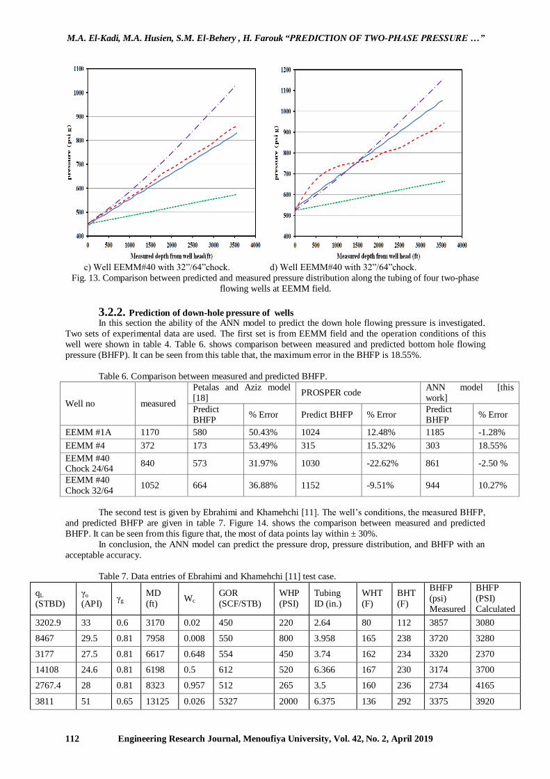
Figure 13 shows a comparison between the
predicted and measured pressure distribution along
the tubing of four flowing wells at EEMM field. It
can be seen from the figure that the ANN model
gives very good results for well EEMM#1-A Fig.
(13 a) followed by PROSPER code. Thus,
PROSPER code and Petalas and Aziz model under-
estimated the pressure along the well tubing. For the second and third cases Fig. (13 b,c), all the
tested models under-estimated the pressure
distribution with PROSPER code and ANN model
very close to each other and close to the measured
data. For the last case, shown in Fig. (13 d), the
PROSPER code over-estimated the pressure
distribution while the other two models under-
estimated it.
M.A. El-Kadi, M.A. Husien, S.M. El-Behery , H. Farouk “PREDICTION OF TWO-PHASE PRESSURE …”
Engineering Research Journal, Menoufiya University, Vol. 42, No. 2, April 2019
111
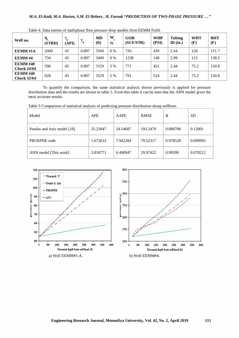
Table 4. Data entries of multiphase flow pressure drop models from EEMM Field.
Well no. q
L
(STBD)
γo
(API) γ
g MD
(ft)
Wc
%
GOR
(SCF/STB) WHP
(PSI) Tubing
ID (in.) WHT
(F) BHT
(F)
EEMM #1A 2000 54 0.897 0453 0 % 645 543 4455 120 14146
EEMM #4 734 45 0.897 3400 0 % 1238 140 2.99 115 138.5
EEMM #40 Chock 24/64
596 45 0.897 0443 5 % 771 451 2.44 75.2 150.8
EEMM #40 Chock 32/64
628 45 0.897 3529 5 % 791 524 2.44 75.2 150.8
To quantify the comparison, the same statistical analysis shown previously is applied for pressure
distribution data and the results are shown in table 5. From this table it can be seen that the ANN model gives the
most accurate results.
Table 5 Comparison of statistical analysis of predicting pressure distribution along wellbore.
Model APE AAPE RMSE R SD
Petalas and Aziz model [18] 25.23047 24.54687 193.2479 0.880708 0.12801
PROSPER code 1.673633 7.942284 79.52317 0.978538 0.099993
ANN model [This work] 3.818771 6.490947 29.97422 0.99599 0.078212
a) Well EEMM#1-A. b) Well EEMM#4.
M.A. El-Kadi, M.A. Husien, S.M. El-Behery , H. Farouk “PREDICTION OF TWO-PHASE PRESSURE …”
Engineering Research Journal, Menoufiya University, Vol. 42, No. 2, April 2019
112
c) Well EEMM#40 with 32”/64”chock. d) Well EEMM#40 with 32”/64”chock.
Fig. 13. Comparison between predicted and measured pressure distribution along the tubing of four two-phase
flowing wells at EEMM field.
3.2.2. Prediction of down-hole pressure of wells In this section the ability of the ANN model to predict the down hole flowing pressure is investigated.
Two sets of experimental data are used. The first set is from EEMM field and the operation conditions of this
well were shown in table 4. Table 6. shows comparison between measured and predicted bottom hole flowing
pressure (BHFP). It can be seen from this table that, the maximum error in the BHFP is 18.55%.
Table 6. Comparison between measured and predicted BHFP.
Well no measured
Petalas and Aziz model
[18] PROSPER code
ANN model [this
work]
Predict
BHFP % Error Predict BHFP % Error
Predict
BHFP % Error
EEMM #1A 1170 580 50.43% 1024 12.48% 1185 -1.28%
EEMM #4 372 173 53.49% 315 15.32% 303 18.55%
EEMM #40 Chock 24/64
840 573 31.97% 1030 -22.62% 861 -2.50 %
EEMM #40 Chock 32/64
1052 664 36.88% 1152 -9.51% 944 10.27%
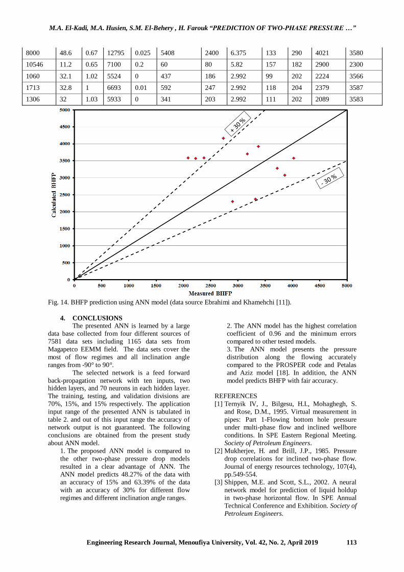
The second test is given by Ebrahimi and Khamehchi [11]. The well’s conditions, the measured BHFP,
and predicted BHFP are given in table 7. Figure 14. shows the comparison between measured and predicted
BHFP. It can be seen from this figure that, the most of data points lay within ± 30%.
In conclusion, the ANN model can predict the pressure drop, pressure distribution, and BHFP with an
acceptable accuracy.
Table 7. Data entries of Ebrahimi and Khamehchi [11] test case.
qL
(STBD)
γo
(API) γg
MD
(ft) Wc
GOR
(SCF/STB)
WHP
(PSI)
Tubing
ID (in.)
WHT
(F)
BHT
(F)
BHFP
(psi)
Measured
BHFP
(PSI)
Calculated
3202.9 33 0.6 3170 0.02 450 220 2.64 80 112 3857 3080
8467 29.5 0.81 7958 0.008 550 800 3.958 165 238 3720 3280
3177 27.5 0.81 6617 0.648 554 450 3.74 162 234 3320 2370
14108 24.6 0.81 6198 0.5 612 520 6.366 167 230 3174 3700
2767.4 28 0.81 8323 0.957 512 265 3.5 160 236 2734 4165
3811 51 0.65 13125 0.026 5327 2000 6.375 136 292 3375 3920
M.A. El-Kadi, M.A. Husien, S.M. El-Behery , H. Farouk “PREDICTION OF TWO-PHASE PRESSURE …”
Engineering Research Journal, Menoufiya University, Vol. 42, No. 2, April 2019
113
8000 48.6 0.67 12795 0.025 5408 2400 6.375 133 290 4021 3580
10546 11.2 0.65 7100 0.2 60 80 5.82 157 182 2900 2300
1060 32.1 1.02 5524 0 437 186 2.992 99 202 2224 3566
1713 32.8 1 6693 0.01 592 247 2.992 118 204 2379 3587
1306 32 1.03 5933 0 341 203 2.992 111 202 2089 3583
Fig. 14. BHFP prediction using ANN model (data source Ebrahimi and Khamehchi [11]).
4. CONCLUSIONS The presented ANN is learned by a large
data base collected from four different sources of
7581 data sets including 1165 data sets from
Magapetco EEMM field. The data sets cover the
most of flow regimes and all inclination angle
ranges from -90° to 90°.
The selected network is a feed forward
back-propagation network with ten inputs, two hidden layers, and 70 neurons in each hidden layer.
The training, testing, and validation divisions are
70%, 15%, and 15% respectively. The application
input range of the presented ANN is tabulated in
table 2. and out of this input range the accuracy of
network output is not guaranteed. The following
conclusions are obtained from the present study
about ANN model.
1. The proposed ANN model is compared to
the other two-phase pressure drop models
resulted in a clear advantage of ANN. The
ANN model predicts 48.27% of the data with
an accuracy of 15% and 63.39% of the data
with an accuracy of 30% for different flow
regimes and different inclination angle ranges.
2. The ANN model has the highest correlation
coefficient of 0.96 and the minimum errors
compared to other tested models.
3. The ANN model presents the pressure
distribution along the flowing accurately
compared to the PROSPER code and Petalas
and Aziz model [18]. In addition, the ANN
model predicts BHFP with fair accuracy.
REFERENCES
[1] Ternyik IV, J., Bilgesu, H.I., Mohaghegh, S.
and Rose, D.M., 1995. Virtual measurement in
pipes: Part 1-Flowing bottom hole pressure
under multi-phase flow and inclined wellbore
conditions. In SPE Eastern Regional Meeting.
Society of Petroleum Engineers.
[2] Mukherjee, H. and Brill, J.P., 1985. Pressure
drop correlations for inclined two-phase flow.
Journal of energy resources technology, 107(4),
pp.549-554.
[3] Shippen, M.E. and Scott, S.L., 2002. A neural
network model for prediction of liquid holdup
in two-phase horizontal flow. In SPE Annual
Technical Conference and Exhibition. Society of
Petroleum Engineers.
M.A. El-Kadi, M.A. Husien, S.M. El-Behery , H. Farouk “PREDICTION OF TWO-PHASE PRESSURE …”
Engineering Research Journal, Menoufiya University, Vol. 42, No. 2, April 2019
114
[4] Osman, E.S.A., 2004. Artificial neural network
models for identifying flow regimes and
predicting liquid holdup in horizontal
multiphase flow. SPE production & facilities,
19(01), pp.33-40.
[5] Osman, E.S.A., Ayoub, M.A. and Aggour,
M.A., 2005. An artificial neural network model
for predicting bottomhole flowing pressure in
vertical multiphase flow. In SPE Middle East
Oil and Gas Show and Conference. Society of
Petroleum Engineers. [6] Ozbayoglu, M.E. and Ozbayoglu, M.A., 2007.
Flow pattern and frictional-pressure-loss
estimation using neural networks for UBD
operations. In IADC/SPE Managed Pressure
Drilling & Underbalanced Operations. Society
of Petroleum Engineers.
[7] Mohammadpoor, M., Shahbazi, K., Torabi, F.,
Firouz, Q. and Reza, A., 2010. A new
methodology for prediction of bottomhole
flowing pressure in vertical multiphase flow in
iranian oil fields using Artificial Neural
Networks (ANNs). In SPE Latin American and
Caribbean Petroleum Engineering Conference.
Society of Petroleum Engineers.
[8] Ashena, R., Moghadasi, J., Ghalambor, A.,
Bataee, M., Ashena, R. and Feghhi, A., 2010.
Neural networks in BHCP prediction performed much better than mechanistic models. In
International Oil and Gas Conference and
Exhibition in China. Society of Petroleum
Engineers.
[9] Adebayo, A.R., Abdulraheem, A. and Al-
Shammari, A.T., 2013. Promises of Artificial
Intelligence Techniques in Reducing Errors in
Complex Flow and Pressure Losses
Calculations in Multiphase Fluid Flow in Oil
Wells. In SPE Nigeria Annual International
Conference and Exhibition. Society of
Petroleum Engineers.
[10] Li, X., Miskimins, J. and Hoffman, B.T., 2014.
A combined bottom-hole pressure calculation
procedure using multiphase correlations and
artificial neural network models. In SPE Annual
Technical Conference and Exhibition. Society of Petroleum Engineers.
[11] Ebrahimi, A. and Khamehchi, E., 2015. A
robust model for computing pressure drop in
vertical multiphase flow. Journal of Natural
Gas Science and Engineering, 26, pp.1306-
.1316
[12] Demuth, H., Beale, M. and Hagan, M., 2008.
Neural network toolbox™ 6. User’s guide
[13] Ali, S. F., 2009. Two-phase flow in a large
diameter vertical riser. PhD Thesis, School of
Engineering, Cranfield University.
[14] Gray, H. E. 1978. Vertical flow correlation – gas wells. User's manual for API 14B, SSCSV
Sizing Computer Program. second edition, API
appendix B, 38-41
[15] Beggs, D.H. and Brill, J.P., 1973. A study of
two-phase flow in inclined pipes. Journal of
Petroleum technology, 25(05), pp.607-617.
[16] Duns Jr, H. and Ros, N.C.J., 1963. Vertical
flow of gas and liquid mixtures in wells. In 6th
world petroleum congress, Frankfurt, Section II,
22-PD6
[17] Mukherjee, H. and Brill, J.P., 1985. Pressure
drop correlations for inclined two-phase flow.
Journal of energy resources technology, 107(4),
pp.549-554.
[18] Petalas, N. and Aziz, K., 1998. A mechanistic
model for multiphase flow in pipes. In Annual
Technical Meeting. Petroleum Society of Canada.
[19] Petalas, N. and Aziz, K., 1995. Stanford
Multiphase Flow Database - User’s manual
Version 2. Petroleum Engineering Dept.,
Stanford University, California, USA.
[20] Meng, W., 1999. Low liquid loading gas-
liquid two-phase flow in near-horizontal pipes.
PhD thesis, U. of Tulsa, Tulsa, Oklahoma,
USA.
[21] Beggs, H.D., 1973. An experimental study of
two-phase flow in inclined pipes. PhD thesis, U.
of Tulsa, Tulsa, Oklahoma, USA.
Recommended