Calhoun: The NPS Institutional Archive
Theses and Dissertations Thesis Collection
2004-06
Prediction of instantaneous currents in San Diego
Bay for naval applications
Armstrong, Albert E.
Monterey, California. Naval Postgraduate School
http://hdl.handle.net/10945/1612
NAVAL
POSTGRADUATE SCHOOL
MONTEREY, CALIFORNIA
THESIS
Approved for public release; distribution is unlimited.
PREDICTION OF INSTANTANEOUS CURRENTS IN SAN DIEGO BAY FOR NAVAL APPLICATIONS
by
Albert E. Armstrong
June 2004
Thesis Advisor: Peter C. Chu Second Reader: Steven D. Haeger

THIS PAGE INTENTIONALLY LEFT BLANK
i
REPORT DOCUMENTATION PAGE Form Approved OMB No. 0704-0188 Public reporting burden for this collection of information is estimated to average 1 hour per response, including the time for reviewing instruction, searching existing data sources, gathering and maintaining the data needed, and completing and reviewing the collection of information. Send comments regarding this burden estimate or any other aspect of this collection of information, including suggestions for reducing this burden, to Washington headquarters Services, Directorate for Information Operations and Reports, 1215 Jefferson Davis Highway, Suite 1204, Arlington, VA 22202-4302, and to the Office of Management and Budget, Paperwork Reduction Project (0704-0188) Washington DC 20503. 1. AGENCY USE ONLY (Leave blank)
2. REPORT DATE June 2004
3. REPORT TYPE AND DATES COVERED Master’s Thesis
4. TITLE AND SUBTITLE: Investigation of Instantaneous Currents in San Diego Bay for Naval Applications 6. AUTHOR(S) Armstrong, Albert E.
5. FUNDING NUMBERS
7. PERFORMING ORGANIZATION NAME(S) AND ADDRESS(ES) Naval Postgraduate School Monterey, CA 93943-5000
8. PERFORMING ORGANIZATION REPORT NUMBER
9. SPONSORING /MONITORING AGENCY NAME(S) AND ADDRESS(ES) Naval Oceanographic Office
10. SPONSORING/MONITORING AGENCY REPORT NUMBER
11. SUPPLEMENTARY NOTES The views expressed in this thesis are those of the author and do not reflect the official policy or position of the Department of Defense or the U.S. Government. 12a. DISTRIBUTION / AVAILABILITY STATEMENT Approved for public release; distribution is unlimited.
12b. DISTRIBUTION CODE
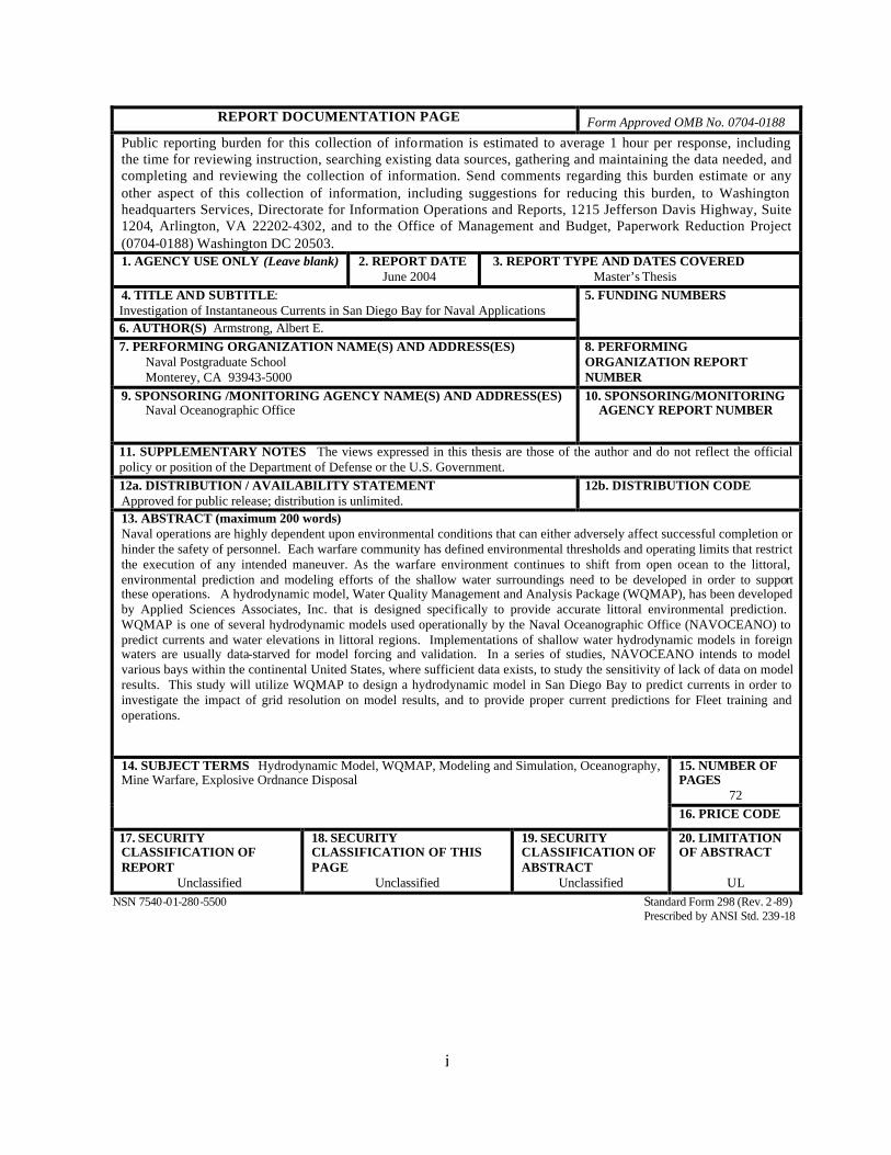
13. ABSTRACT (maximum 200 words) Naval operations are highly dependent upon environmental conditions that can either adversely affect successful completion or hinder the safety of personnel. Each warfare community has defined environmental thresholds and operating limits that restrict the execution of any intended maneuver. As the warfare environment continues to shift from open ocean to the littoral, environmental prediction and modeling efforts of the shallow water surroundings need to be developed in order to support these operations. A hydrodynamic model, Water Quality Management and Analysis Package (WQMAP), has been developed by Applied Sciences Associates, Inc. that is designed specifically to provide accurate littoral environmental prediction. WQMAP is one of several hydrodynamic models used operationally by the Naval Oceanographic Office (NAVOCEANO) to predict currents and water elevations in littoral regions. Implementations of shallow water hydrodynamic models in foreign waters are usually data-starved for model forcing and validation. In a series of studies, NAVOCEANO intends to model various bays within the continental United States, where sufficient data exists, to study the sensitivity of lack of data on model results. This study will utilize WQMAP to design a hydrodynamic model in San Diego Bay to predict currents in order to investigate the impact of grid resolution on model results, and to provide proper current predictions for Fleet training and operations.
15. NUMBER OF PAGES
72
14. SUBJECT TERMS Hydrodynamic Model, WQMAP, Modeling and Simulation, Oceanography, Mine Warfare, Explosive Ordnance Disposal
16. PRICE CODE
17. SECURITY CLASSIFICATION OF REPORT
Unclassified
18. SECURITY CLASSIFICATION OF THIS PAGE
Unclassified
19. SECURITY CLASSIFICATION OF ABSTRACT
Unclassified
20. LIMITATION OF ABSTRACT
UL
NSN 7540-01-280-5500 Standard Form 298 (Rev. 2-89) Prescribed by ANSI Std. 239-18

ii
THIS PAGE INTENTIONALLY LEFT BLANK

iii
Approved for public release; distribution is unlimited.
PREDICTION OF INSTANTANEOUS CURRENTS IN SAN DIEGO BAY FOR NAVAL APPLICATIONS
Albert E. Armstrong
Lieutenant, United States Navy B.S., The University of Memphis, 1998
Submitted in partial fulfillment of the requirements for the degree of
MASTER OF SCIENCE IN METEOROLOGY AND PHYSICAL OCEANOGRAPHY
from the
NAVAL POSTGRADUATE SCHOOL June 2004
Author: Albert E. Armstrong
Approved by: Peter C. Chu
Thesis Advisor
Steven D. Haeger Second Reader/Co-Advisor
Mary L. Batteen Chairman, Department of Oceanography

iv
THIS PAGE INTENTIONALLY LEFT BLANK
v
ABSTRACT
Naval operations are highly dependent upon environmental conditions that can
either adversely affect successful completion or hinder the safety of personnel. Each
warfare community has defined environmental thresholds and operating limits that
restrict the execution of any intended maneuver. As the warfare environment continues to
shift from open ocean to the littoral, environmental prediction and modeling efforts of the
shallow water surroundings need to be developed in order to support these operations. A
hydrodynamic model, Water Quality Management and Analysis Package (WQMAP), has
been developed by Applied Sciences Associates, Inc. that is designed specifically to
provide accurate littoral environmental prediction. WQMAP is one of several
hydrodynamic models used operationally by the Naval Oceanographic Office
(NAVOCEANO) to predict currents and water elevations in littoral regions.
Implementations of shallow water hydrodynamic models in foreign waters are usually
data-starved for model forcing and validation. In a series of studies, NAVOCEANO
intends to model various bays within the continental United States, where sufficient data
exists, to study the sensitivity of lack of data on model results. This study will utilize
WQMAP to design a hydrodynamic model in San Diego Bay to predict currents in order
to investigate the impact of grid resolution on model results, and to provide proper
current predictions for Fleet training and operations.

vi
THIS PAGE INTENTIONALLY LEFT BLANK
vii
TABLE OF CONTENTS
I. INTRODUCTION .......................................................................................................1 A. OVERVIEW.....................................................................................................1 B. WATER QUALITY MAPPING AND ANALYSIS PROGRAM
(WQMAP) ........................................................................................................2 1. WQMAP as a Hydrodynamic Model Choice ....................................2 2. WQMAP as Windows Platform .........................................................2
a. Geographic Information System (GIS)....................................3 b. Graphical User Interface (GUI)...............................................3
C. PURPOSE.........................................................................................................4
II. MODEL ........................................................................................................................5 A. HYBRID ORTHORGONAL CURVILINEAR-TERRAIN
FOLLOWING COORDINATE SYSTEM ....................................................5 B. GOVERNING EQUATIONS .........................................................................5 C. VERTICAL AVERAGED MODE.................................................................7 D. MODEL NUMERICS .....................................................................................7
III. BOUNDARY FITTED GRID CREATION ............................................................11 A. CREATING A NEW SCENARIO ...............................................................11 B. CREATING THE BOUNDARY FITTED GRID.......................................11
IV. DATA AND METHODS...........................................................................................21 A. DATA COLLECTION ..................................................................................21
1. Forcing Data .......................................................................................21 2. Verification Data................................................................................23 3. Bathymetry .........................................................................................26
B. HYDRODYNAMIC MODEL EXECUTION .............................................27 1. Model Run Control ............................................................................27 2. Model Parameters ..............................................................................27 3. Physical Parameters ..........................................................................28 4. Output Time Series Sites...................................................................28 5. GUI Results ........................................................................................30
C. DATA PROCESSING...................................................................................32 1. WQMAP Output Files.......................................................................32 2. Rotational Matrix ..............................................................................33
IV. RESULTS ...................................................................................................................35 A. DIFFERENCE BETWEEN DIFFERENT RESOLUTION GRIDS.........35 B. COMPARISON OF TIDE TABLE DATA TO MODELED
CURRENTS ...................................................................................................38 C. STATIONS FURTHER FROM BAY ENTRANCE ..................................41
V. CONCLUSIONS........................................................................................................45 A. NEED FOR ADCP DATA ............................................................................45 B. APPLICATION OF MODELED RESULTS ..............................................45

viii
1. MIW Exercise.....................................................................................45 2. EOD Operation..................................................................................49
C. FUTURE APPLICATION USING FLEET SURVEY TEAM ASSETS..52
LIST OF REFERENCES ......................................................................................................53
INITIAL DISTRIBUTION LIST.........................................................................................55
ix
LIST OF FIGURES
Figure 1. Arakawa ‘C’ Grid. .............................................................................................8 Figure 2. Grid Representation. ..........................................................................................9 Figure 3. Initial Grid Creation. ........................................................................................13 Figure 4. Interpolating Grid Boundaries. ........................................................................14 Figure 5. Forming Bay Symmetry. .................................................................................15 Figure 6. Aligning Grid to San Diego Bay Boundaries. .................................................16 Figure 7. Coarse Boundary Fitted Grid ...........................................................................17 Figure 8. Medium Boundary Fitted Grid ........................................................................18 Figure 9. Fine Boundary Fitted Grid ...............................................................................19 Figure 10. San Diego Bay Bathymetry .............................................................................26 Figure 11. Time Series Sites .............................................................................................29 Figure 12. Animation Screenshot of WQMAP Modeled Current 0600 January 6th,
2004 .................................................................................................................30 Figure 13. Station 1 WQMAP Modeled Current January 2004 ........................................31 Figure 14. Rotational Matrix Visualization. .....................................................................33 Figure 15. WQMAP Modeled Currents for Station 4 (San Diego Bay Entrance) ............36 Figure 16. Difference in Modeled Current Between Grid Resolutions at Station 4. ........37 Figure 17. WQMAP Modeled Currents and NOAA Tide Table for San Diego Bay
Entrance. ..........................................................................................................39 Figure 18. Plot of Verified Six Minute Water Level VS NOAA Tide Table Data for
January 2004. ...................................................................................................40 Figure 19. Station 4 Modeled Currents vs NOAA Tide Table Data for San Diego Bay
Entrance. ..........................................................................................................42 Figure 20. Station 6 Modeled Currents vs NOAA Tide Table Data for San Diego Bay
Entrance. ..........................................................................................................43 Figure 21. Operational Example of MIW Exercise for 21 January 2004 at Station 4
Using Fictitious Current Threshold of 2.0 knots using NOAA Tide Table Data. .................................................................................................................47
Figure 22. Operational Example of MIW Exercise for 21 January 2004 at Station 4 Using Fictitious Current Threshold of 2.0 knots using WQMAP Fine Resolution Grid Modeled Currents..................................................................48
Figure 23. Operational Example of EOD Exercise for 21 January 2004 at Station 4 Using Fictitious Cur rent Threshold of 0.5 knots using NOAA Tide Table Data. .................................................................................................................50
Figure 24. Operational Example of EOD Exercise for 21 January 2004 at Station 4 Using Fictitious Current Threshold of 0.5 knots using WQMAP Fine Resolution Grid Modeled Currents..................................................................51

x
THIS PAGE INTENTIONALLY LEFT BLANK

xi
LIST OF TABLES
Table 1. NOAA/NOS Verified 6 minute Water Level Data (Truncated) for Station 9410170 (San Diego Bay, Ballast Point.) ........................................................22
Table 2. NOAA/NOS Tidal Water Level Data for Station 9410170 (San Diego Bay, Ballast Point.) ..........................................................................................24
Table 3. NOAA/NOS Tidal Current Data for Station 9410170 (San Diego Bay, Ballast Point.). .................................................................................................25
Table 4. WQMAP Modeled U Velocity for Station 1, Truncated Output File..............32

xii
THIS PAGE INTENTIONALLY LEFT BLANK
xiii
ACKNOWLEDGMENTS
Funding for this research was provided by the Naval Oceanographic Office,
Stennis Space Center, Mississippi.
I wish to thank Dr. Peter Chu from Naval Postgraduate School and Mr. Steve
Haeger from the Naval Oceanographic Office for keeping my strong personal interest in
Geospatial Information Systems in mind when they presented this thesis opportunity to
me. I greatly appreciate the hours of personal assistance they provided me when the
modeling process presented unexpected challenges under the time constraints we were
required to work under.
I would also like to thank Mr. Matt Ward from Applied Science Associates, Inc
for the outstanding training he provided on WQMAP grid formation and model
execution. Mr. Ward had only five days to train us on the software package that normally
requires two to three weeks. His mastery of not only WQPMAP, but of coastal
hydrodynamics was pivotal in understanding the intricacies of the project we were
undertaking. He was always available via email and over the phone to help resolve issues
that arose. Without that help, this project would not have been completed on time.
I especially wish to thank my lovely wife, Jody, for her loving support during this
particular challenge. In order to receive orders to the NAVOCEANO’s Hydrography
Program, I was required to graduate one quarter earlier. With the resultant increase in my
academic load as well as the decreased time to finalize my thesis, she had to pick up more
burden during our stay here despite her own full time job and part time schooling. Jody,
thanks for all your hard work so that we both could succeed.

xiv
THIS PAGE INTENTIONALLY LEFT BLANK
1
I. INTRODUCTION
This study consists of a detailed analysis of tidal elevation and current data for
San Diego Bay during the time period from January 1st, 2004 to January 31st, 2004 for the
purpose of predicting the instantaneous currents within San Diego Bay to support for
myriad of naval operations that are limited to water current thresholds. The
hydrodynamic model utilized in analyzing these currents was a commercial off- the-shelf
Windows based application called Water Quality Mapping and Analysis Program
(WQMAP) that was developed Applied Science Associates, Inc. This program was
developed specifically for marine and fresh water modeling applications.
A. OVERVIEW
The execution of any naval operation can be hindered by numerous environmental
factors. Proper planning for these operations includes forecasting the environment of the
area of operations. Each warfare area has defined environmental thresholds and
operating limits that restrict the execution of any intended maneuver. Amphibious
Assault Vehicles (AAV), Mechanized Landing Craft (LCM 6 and LCM 8), Utility
Landing Craft (LCU 1646), AN/SLQ-48 Mine Neutralization Vehicle (MNV) aboard
AVENGER Class Mine Countermeasures Ships (MCM) and OSPREY Class Coastal
Minehunters (MHC), and EOD/Diver operations all have these water current thresholds.
As the warfare environment continues to shift from open ocean to the littoral,
environmental prediction and modeling efforts of the shallow water surroundings need to
be developed in order to support these operations. Present Navy operational current
prediction models consist of Wave Watch 3 (WW3) from Fleet Numerical Meteorology
and Oceanography Command and Navy Layered Ocean Model (NLOM) out of the Naval
Oceanographic Office. Both these models forecast for large scale or global regions and
do not provide output for inner littoral bays and estuaries. A finer resolution model
designed within specific bays is required to support mine warfare and diver operations
within those explicit locations.
2
B. WATER QUALITY MAPPING AND ANALYSIS PROGRAM (WQMAP)
WQMAP is an integrated hydrodynamic and water quality modeling system
designed for use within coastal and fresh water environments. This commercial off- the-
shelf program was developed by Applied Science Associates, Inc. out of Narragansett,
Rhode Island. WQMAP consists of three basic components: a boundary-fitted coordinate
grid creation module, a three-dimensional hydrodynamics model, and a water quality or
pollutant transport model. These models are executed on a boundary fitted grid system.
They can also be operated on any orthogonal curvilinear grid or a rectangular grid, which
are special cases of the boundary fitted grid.
1. WQMAP as a Hydrodynamic Model Choice
The WQMAP hydrodynamic model solves the three dimensional equations of the
conservation of water mass, conservation of momentum, and the salt and energy
equations. These solutions are computed on a spherical, nonorthogonal, boundary fitted
grid system that is applicable for littoral regions and can also be predicted as two
dimensional, vertically averaged circulations. The model can calculate a time varying
field of surface elevations and/or velocity vectors. Environmental forcing inputs include
tides, surface elevations, and wind fields. The model is configured to run in a vertically
averaged mode or as a fully three-dimensional, baroclinic mode. A sigma stretching
system is incorporated to diagram the free surface and bottom to resolve bathymetric
variations. Calculations are achieved on a space-staggered grid system in the horizontal
and a non-staggered system in the vertical.
2. WQMAP as Windows Platform
WQMAP requires an IBM-compatible 486 or better PC running Microsoft
Windows 95 or higher, although a Pentium system is recommended. It also requires a
minimum of 64 megabytes of RAM, 100 megabytes of free hard drive disk space, and a
VGA color monitor. The system permits the user to directly create boundary fitted grid
systems through a user- friendly Windows graphical interface which is controlled by pull
down menus and point and click operations similarly found in most Windows-based
applications. These boundary grids represent the area of interest from which the model
predictions can be displayed in the form of time series plots, vector and contour plots, in
addition to color animated displays. The software is developed for making new

3
applications to any geographic area with remarkable speed and simplicity. Supporting
data is accessed through the location specific data sets, the geographic information
system (GIS), or input through the menu windows.
a. Geographic Information System (GIS)
The program has a GIS base and can be set up for any number of regions
in the world. The embedded GIS permits input, storage, manipulation, and analysis, and
displays geographically referenced information. Moreover, the GIS is quick, interactive,
and simple to use. GIS based data sets from other GIS based programs, such as
ArcView, can be imported and displayed as well. The user can quickly change from one
geographic location to another by simply “pointing” the display to the appropriate data
set. These locations, as in any GIS location, are defined by a base map and a series of
GIS layers of vector or raster data. The GIS can also be used to provide input data to the
models. Everything from the location selection, grid design, selection of forcing data, to
the display of the model run is controlled from the simple GIS user interface.
b. Graphical User Interface (GUI)
The WQMAP graphical interface permits every function (from boundary
fitted grid creations, importation of open boundary conditions, and execution of the
hydrodynamic model, to exporting either graphical or tabular results) to be extremely
effortless. The program allows the user to display the results of any model calculations.
The user opens a defined scenario and selects the variable (currents, temperature, surface
elevation, salinity) and the vertical level. The results can then be animated, using either
vectors or color contours, covering the model simulation period. The animation control
allows forward, step forward, and rewind options. The animations can also be overlaid on
the bathymetric data to allow the user to visualize the relationship between the predicted
values (currents, salinity, and temperature) and the depth. The user can also choose a
section view window (vertical cross section along user selected line) that permits any
variable to be displayed along the section line at the same time as the grid view is
animated. Time series data can also be plotted and exported from this section line as
well.
4
C. PURPOSE
This study is concerned with the analysis of the WQMAP model current
prediction of San Diego Bay. The focus was to characterize and predict the circulation of
the bay where present day Navy operational current models cannot determine such
parameters. If the modeled currents can be accurately determined, then the time frame
where operational thresholds will be exceeded can also be determined, whether the
planned operation is for mine warfare, diver operations, or in many situations, both. The
objectives of this investigation are listed as follows:
• Assess the accuracy of WQMAP in determining current circulations
within San Diego Bay.
• Operationally outline current threshold restrictions on mine warfare and
diving operations for the same modeling period.
• To provide Naval Oceanographic Office an accurate current prediction
boundary fitted grid by which future inner bay naval operations may be
properly planned from.

5
II. MODEL
A. HYBRID ORTHORGONAL CURVILINEAR-TERRAIN FOLLOWING COORDINATE SYSTEM
Let ( , , zϕ λ ) be the latitude, longitude, and height, and ( , ,ξ η σ ) be a hybrid
coordinate system with a generalized orthogonal curvilinear coordinate system ( ,ξ η ) in
the horizontal and terrain-following σ -coordinate in the vertical. The metric coefficients
connecting ( ,φ λ ) to ( ,ξ η ) are defined by
2 2 211 ( ) cos ( )g
λ ϕφ
ξ ξ∂ ∂
= +∂ ∂
, (1)
2 2 222 ( ) cos ( )g
λ ϕη η
∂ ∂= +
∂ ∂ . (2)
Let (ζ , H) be the surface elevation and bathymetry. D = H + ζ , is the total
water depth. The σ - and z-coordinates are connected by
z H
Hσ
ζ+
=+
, (3)
which makes 1σ = for the ocean surface and 0σ = for the ocean bottom.
B. GOVERNING EQUATIONS
The equations of motions and continuity are expressed in a hybrid orthogonal
curvilinear-terrain following coordinate system ( , ,ξ η σ ) with (u,v,ω ) being the
corresponding velocity components. In this coordinate system, the basic dynamical
system is represented by Kantha and Clayson (2000).
( ) ( )22 11
11 22 11 22 0uD g vD g
R g g R g gtζ ω
ξ η σ
∂ ∂∂ ∂+ + + =
∂ ∂ ∂ ∂, (4)
which is the continuity equation,

6
( ) ( ) ( ) ( )222 11 11 222
11 22
0
011
1
1,v
u D g uvD g g guDuvD v fDV
t g g
u gD D D ufDv d A
D DR g σ
ξ η η ξ
ω ζ ρ σ ρσ
σ ξ ρ ξ ξ σ σ σ
∂ ∂ ∂ ∂∂ + + + − − ∂ ∂ ∂ ∂ ∂
∂ ∂ ∂ ∂ ∂ ∂ ∂ + − = − + − + ∂ ∂ ∂ ∂ ∂ ∂ ∂ ∫
(5)
which is the momentum equation in ξ -direction,
( ) ( ) ( ) ( )222 11 22 112
11 22
0
022
1
1,v
uvD g v D g g gvDuvD u fDV
t g g
v gD D D vfDu d A
D DR g σ
ξ η ξ η
ω ζ ρ σ ρσ
σ ξ ρ ξ ξ σ σ σ
∂ ∂ ∂ ∂∂ + + + − + ∂ ∂ ∂ ∂ ∂
∂ ∂ ∂ ∂ ∂ ∂ ∂ + + = − + − + ∂ ∂ ∂ ∂ ∂ ∂ ∂ ∫
(6)
which is the momentum equation in η -direction. Here, R is the earth radius; 0ρ (= 1025
kg/m3) is the characteristic density for the seawater; f is the Coriolis parameter, g is the
acceleration due to gravity, Av is the vertical eddy viscosity. The transport equations for
temperature and salinity are represented by
2 2
2 2 2 2 211 2211 22
1 1 1,h h v
S u S v S S S S Sw D D D
t R g R g DR g R gξ η σ ξ η σ σ ∂ ∂ ∂ ∂ ∂ ∂ ∂ ∂ + + + = + + ∂ ∂ ∂ ∂ ∂ ∂ ∂ ∂
(7)
2 2
2 2 2 2 211 2211 22
1 1 1,h h v
T u T v T T T T Tw D D D
t R g R g DR g R gξ η σ ξ η σ σ ∂ ∂ ∂ ∂ ∂ ∂ ∂ ∂ + + + = + + ∂ ∂ ∂ ∂ ∂ ∂ ∂ ∂
(8)
where Dh and Dv are horizontal and vertical diffusivities.
The three-dimensional hydrodynamic equations (4-6), contain both high-speed
external gravity waves and slow propagating internal gravity waves. The equations of
motion are broken up into vertically averaged equations and vertical structure equations,
which are called the exterior and interior modes by the WQMAP documentation,
respectfully. This approach permits the calculation of free surface elevation from the
exterior mode and the three-dimensional currents and thermodynamic properties from the
interior mode. The vertically averaged equations are obtained by integrating equations (4-
6) from s =0 to s =-1.

7
C. VERTICAL AVERAGED MODE
Let (U, V) be the vertically averaged velocity components in ( ,ξ η ) directions.
Vertical integration of (5) and (6) leads to the momentum equations for (U, V),
( ) ( ) ( ) ( )222 11 11 222
11 22
0 0
0 111
1
,
U D g UVD g g gUDUVD V fDV
t g g
gD D Dd
DR g σ
ξ η η ξ
ζ ρ σ ρσ
ξ ρ ξ ξ σ−
∂ ∂ ∂ ∂∂ + + + − − ∂ ∂ ∂ ∂ ∂
∂ ∂ ∂ ∂= − + − ∂ ∂ ∂ ∂
∫ ∫
(9)
( ) ( ) ( ) ( )222 11 22 112
11 22
0 0
0 122
1
.
UVD g V D g g gVDUVD U fDV
t g g
gD D Dd
DR g σ
ξ η ξ η
ζ ρ σ ρσ
η ρ η η σ−
∂ ∂ ∂ ∂∂ + + + − + ∂ ∂ ∂ ∂ ∂
∂ ∂ ∂ ∂= − + − ∂ ∂ ∂ ∂
∫ ∫
(10)
Vertical integration of (4) leads to
( ) ( )22 11
11 22 0UD g VD g
R g gtζ
ξ η
∂ ∂∂+ + =
∂ ∂ ∂, (11)
which is the continuity equation for the vertically averaged mode.
D. MODEL NUMERICS
The surface elevation is solved implicitly whereas the density gradient, bottom
stress, Coriolis, and advective terms are solved explicitly. The two-dimensional
vertically averaged equations of continuity and motion are solved semi- implicitly. The
momentum equations are substituted into the continuity equation to obtain a Helmholtz
equation in terms of surface elevation. A staggered spatial discretization is established
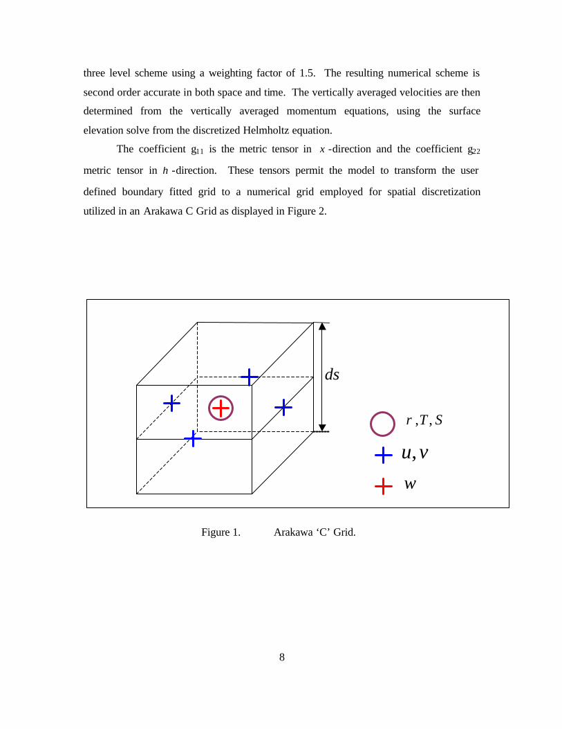
for the Arakawa Grid C system (Arakawa and Lamb, 1977) as displayed in Figure 1. The
u and v velocities are defined, within a layer, in a staggered orientation in the horizontal
direction, but determined at the center in the vertical direction. The vertical velocity ω is
similarly defined at the center of a layer in the vertical direction in the center of the cell in
the horizontal direction. The variables density, temperature, salinity, eddy diffusivity and
eddy viscosity are also defined at the center of the cell. Time is discretized by means of a
8
three level scheme using a weighting factor of 1.5. The resulting numerical scheme is
second order accurate in both space and time. The vertically averaged velocities are then
determined from the vertically averaged momentum equations, using the surface
elevation solve from the discretized Helmholtz equation.
The coefficient g11 is the metric tensor in ξ -direction and the coefficient g22
metric tensor in η -direction. These tensors permit the model to transform the user
defined boundary fitted grid to a numerical grid employed for spatial discretization
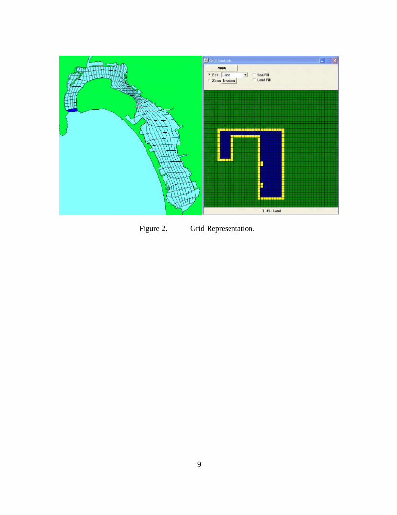
utilized in an Arakawa C Grid as displayed in Figure 2.
Figure 1. Arakawa ‘C’ Grid.
, ,T Sρ
dσ
w
,u v
9
Figure 2. Grid Representation.

10
THIS PAGE INTENTIONALLY LEFT BLANK
11
III. BOUNDARY FITTED GRID CREATION
A. CREATING A NEW SCENARIO
The start of this process is to create a new scenario for the project. Scenarios
consist of the same geographic location to be modeled. Each individual scenario can be
either a hydrodynamic model or mass transport model (e.g., pollution tracking). The
particular scenario can consist of either a two dimensional (2-D) vertically averaged
model or a three dimensional (3-D) model. In addition, each saved scenario tracks the
grid, bathymetry, open boundary forcing, and time frame of that particular scenario. If it
was desired to run similar conditions but use different designed grids, then separated
scenarios must be saved to keep these distinctions on record. Under the “File’ menu,
‘New Scenario’ needs to be selected to start the process. Under a separate window the
choice of either hydrodynamic model or mass transport model is made, as well as
scenario name, and either a 2-D or 3-D model is to be used. If the model is 3-D, then the
number of sigma levels also needs to be identified. For the purposes of this study, a 2-D
hydrodynamic model was selected.
B. CREATING THE BOUNDARY FITTED GRID
Since WQMAP is a geospatial information system, the region which is to be
hydrodynamically modeled needs to be identified with the appropriate map location file
displayed as a GIS layer. WQMAP is supplied with one base map, or location, with the
ability to input additional areas depending on the need of the user. This base map serves
as the largest domain over which the hydrodynamic model will be implemented. Model
locations vary from small rivers, lakes and estuarine systems with scales of kilometers, to
bays, seas, and the continental shelf, with scales of tens to hundreds of kilometers. For
each location, a geo-referenced shoreline and bathymetry is created from either magnetic
data or charts. Base maps of small spatial extent may contain high-resolution
characteristics (harbor shapes, piers, etc.). Conversely, large spatial extent base maps
have less detail. For this study a small spatial extent ASA map file (.bdm) for the San
Diego Bay was utilized.
12
Initial grid creation is rather simple. From the ‘Grid’ pull down menu, ‘New
Grid’ is selected. The user clicks and drags the mouse drawing a box over the area to be
modeled. A grid parameter window opens where, at a minimum, the grid resolution
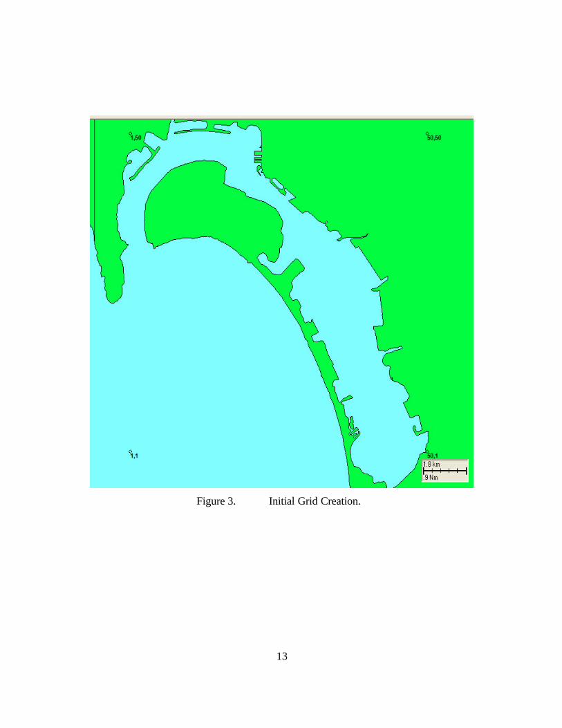
(Imax and Jmax) and the grid name need to be identified. The first grid generated was a
coarse 50 by 50 grid. The four corners of the box identify the grid boundaries starting
with the lower left at as (1,1), the upper left as (1,50), the lower right as (50,1) and the
upper right at (50,50) as seen in Figure 3. The grid end points can then connected by
selecting an ‘Interpolate Points’ command from either the ‘Grid’ pull down menu or by
right clicking.
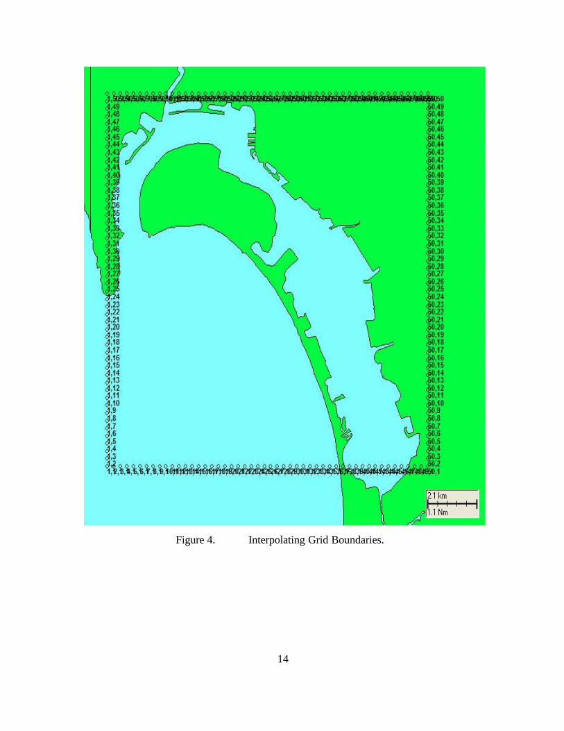
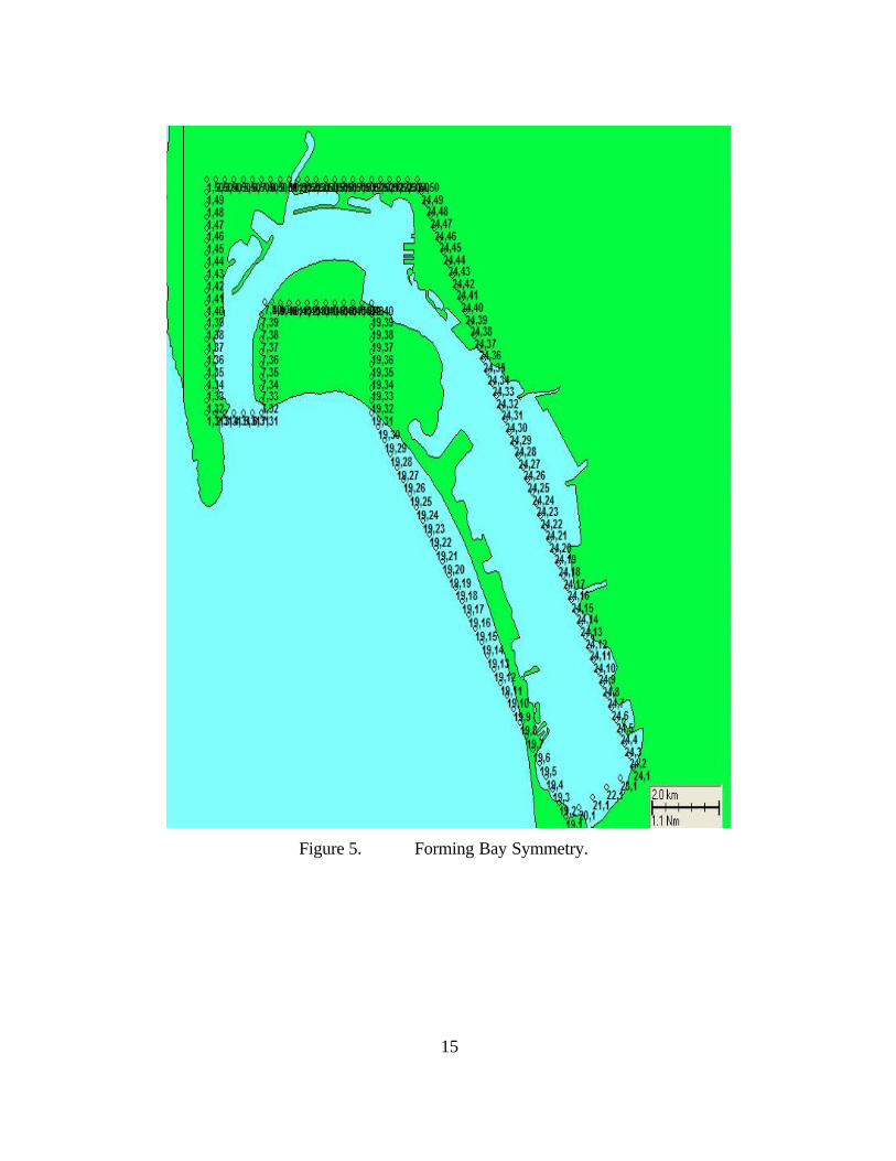
Once the grid borders are established, as displayed in Figure 4, the process
becomes more complex. The user must strategically shape the grid to the general
symmetry of the bay itself. This process requires the user to mentally picture the bay as a
rectangular construct. The user accomplishes this by interpolating additional points
around the general shape of the bay, and then strategically removing the excess over land
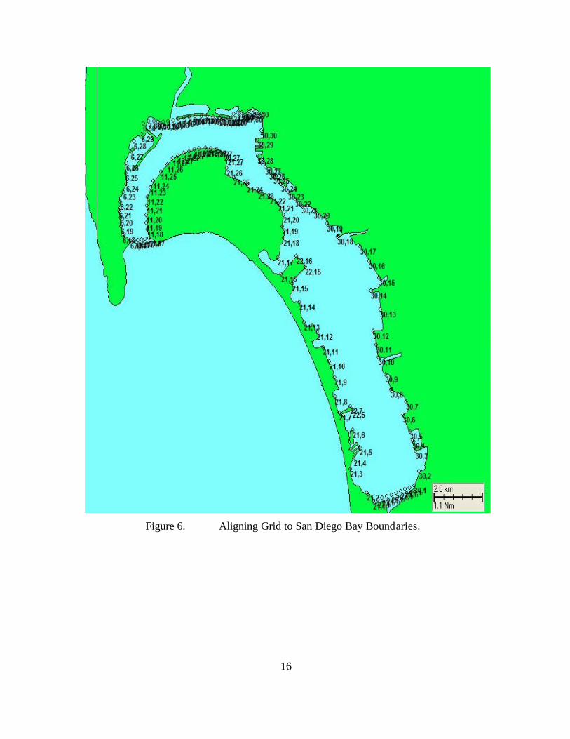
(Figure 5). Once the general shape is determined, the user moves the symmetric grid
points to conform to the bay’s actual boundaries. Finally, the grid is ready to be
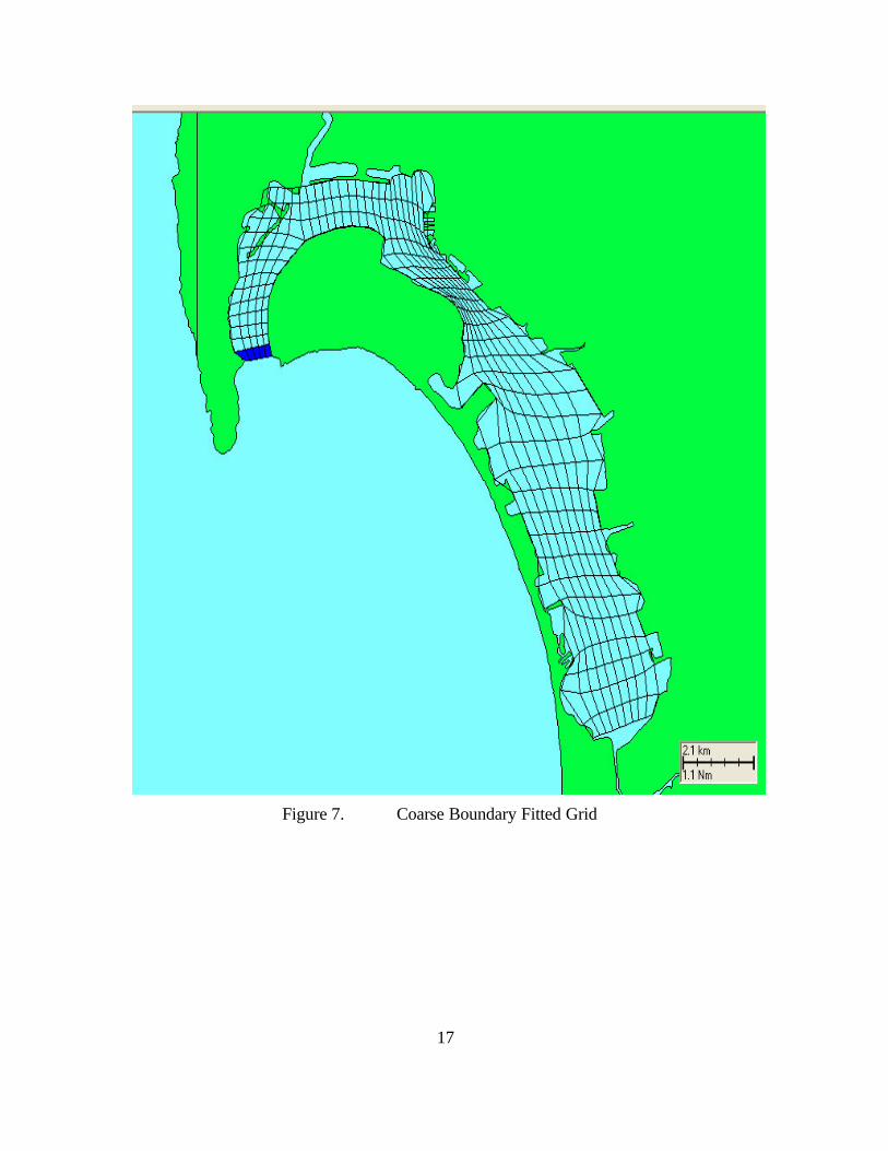
processed. Under the ‘Grid’ pull down menu, the user selects ‘Run Gridding Model’.
WQMAP then creates the entire boundary fitted grid while calculating the spatial
transform tensors of g11 and g22 for each grid cell. The boundary fitted grid that is seen
by the user (Figure 7) is mathematically linked to the spatial discretized Arakawa C Grid
as displayed in Figure 2.
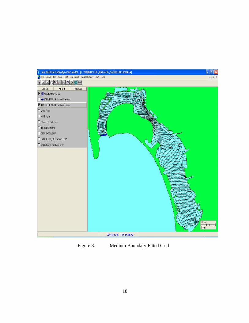
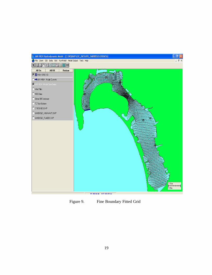
Three separate grids were created for this study: a coarse resolution 50 by 50 grid
(Figure 7), a medium resolution 100 by 100 grid (Figure 8), and a fine resolution 150 by
150 grid (Figure 9).
13
Figure 3. Initial Grid Creation.
14
Figure 4. Interpolating Grid Boundaries.
15
Figure 5. Forming Bay Symmetry.
16
Figure 6. Aligning Grid to San Diego Bay Boundaries.
17
Figure 7. Coarse Boundary Fitted Grid
18
Figure 8. Medium Boundary Fitted Grid
19
Figure 9. Fine Boundary Fitted Grid

20
THIS PAGE INTENTIONALLY LEFT BLANK
21
IV. DATA AND METHODS
A. DATA COLLECTION
1. Forcing Data
The blue shaded cells of Figures 7, 8, and 9 are defined as the open boundary
conditions with the model. The land boundaries are assumed impermeable; hence the
normal component of the velocity at those boundaries is set to zero. Tidal harmonic
constituents or sea surface elevation can be an input as a function of time along the open
boundaries. Such elevation data for the entrance to San Diego Bay was available the
National Oceanographic and Atmospheric Administration’s (NOAA) Center for
Operational Oceanographic Products and Services (CO-OPS) website. A search was
conducted for verified six-minute elevation data from time 0000 on 01 January 2004 to
2354 on 31 January 2004 for the San Diego Bay entrance (Station Identification Number
9410170). An example of the beginning of the data file that was returned is displayed in
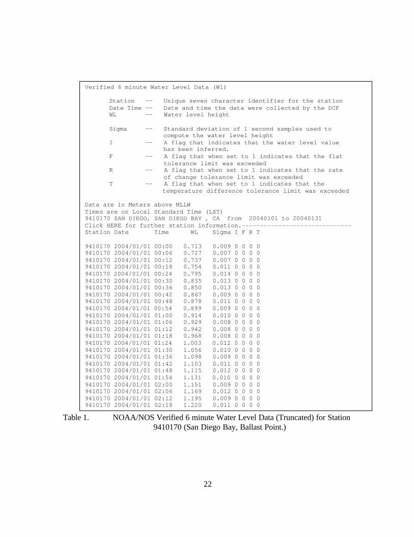
Table 1. Since this data was sampled once every 6 minutes for the month of January, the
data set consisted of 7,440 lines of observed elevation data points. The file must be
formatted such that WQMAP can import it as an Open Boundary Tidal Forcing file (.hst).
The HST file is a time series file for tidal forcing, salinity and temperature to be linked to
the blue open boundary cells. The HST layout consists of an ASCII format of year,
month, day, hour, minutes, elevation (m), salinity (ppt) and temperature (°C). The data
can be either comma or space delimited. This study was not concerned with salinity and
temperature advection so those value could be omitted. The first 22 lines of the data file
were deleted as well as the first 8 columns, which was merely the Station Identification
Number. Then column 5 (a slash), column 8 (another slash), and column 14 (a colon)
were replaced with spaces and then saved. Then the new file’s last column was
extracted. A Fast Fourier Transport was then conducted on the data set, and the high
frequency signal that was present within the data set from winds, fronts, etc was filtered
out. This new smoothed elevation data column was reinserted to the file. The file could
then be saved with a *.hst extension and moved to the ‘runhydro’ sub-directory of the
program directory.
22
Verified 6 minute Water Level Data (W1) Station -- Unique seven character identifier for the station Date Time -- Date and time the data were collected by the DCP WL -- Water level height
Sigma -- Standard deviation of 1 second samples used to compute the water level height
I -- A flag that indicates that the water level value has been inferred. F -- A flag that when set to 1 indicates that the flat tolerance limit was exceeded R -- A flag that when set to 1 indicates that the rate of change tolerance limit was exceeded T -- A flag that when set to 1 indicates that the
temperature difference tolerance limit was exceeded
Data are in Meters above MLLW Times are on Local Standard Time (LST) 9410170 SAN DIEGO, SAN DIEGO BAY , CA from 20040101 to 20040131 Click HERE for further station information.------------------------------ Station Date Time WL Sigma I F R T
9410170 2004/01/01 00:00 0.713 0.009 0 0 0 0 9410170 2004/01/01 00:06 0.727 0.007 0 0 0 0 9410170 2004/01/01 00:12 0.737 0.007 0 0 0 0 9410170 2004/01/01 00:18 0.754 0.011 0 0 0 0 9410170 2004/01/01 00:24 0.795 0.014 0 0 0 0 9410170 2004/01/01 00:30 0.835 0.013 0 0 0 0 9410170 2004/01/01 00:36 0.850 0.013 0 0 0 0 9410170 2004/01/01 00:42 0.867 0.009 0 0 0 0 9410170 2004/01/01 00:48 0.878 0.011 0 0 0 0 9410170 2004/01/01 00:54 0.899 0.009 0 0 0 0 9410170 2004/01/01 01:00 0.914 0.010 0 0 0 0 9410170 2004/01/01 01:06 0.929 0.008 0 0 0 0 9410170 2004/01/01 01:12 0.942 0.008 0 0 0 0 9410170 2004/01/01 01:18 0.968 0.008 0 0 0 0 9410170 2004/01/01 01:24 1.003 0.012 0 0 0 0 9410170 2004/01/01 01:30 1.056 0.010 0 0 0 0 9410170 2004/01/01 01:36 1.098 0.009 0 0 0 0 9410170 2004/01/01 01:42 1.103 0.011 0 0 0 0 9410170 2004/01/01 01:48 1.115 0.012 0 0 0 0 9410170 2004/01/01 01:54 1.131 0.010 0 0 0 0 9410170 2004/01/01 02:00 1.151 0.009 0 0 0 0 9410170 2004/01/01 02:06 1.169 0.012 0 0 0 0 9410170 2004/01/01 02:12 1.195 0.009 0 0 0 0 9410170 2004/01/01 02:18 1.220 0.011 0 0 0 0
Table 1. NOAA/NOS Verified 6 minute Water Level Data (Truncated) for Station 9410170 (San Diego Bay, Ballast Point.)
23
2. Verification Data
The original intent of this study was to compare the modeled output of currents
within San Diego Bay from WQMAP to observed current data collected by an Acoustic
Doppler Current Profiler (ADCP) from the same time frame. Such a data source was
identified online with the San Diego Marine Information System (SDMIS). SDMIS has
three ADCPs located with San Diego Bay. The first one was positioned at the SPAWAR
Pier 160/A, the second was at the 10th Avenue Marine Terminal, and the third was
located at the National City Marine Terminal. This information was available live online,
but archived data was not. Contact with SDMIS revealed that the company InterOcean
Systems Inc maintained the ADCPs and the database. Contact with the InterOcean
Systems Inc Data Manager revealed that the T1 connection connecting the ACDPs to the
mainframe computer was down for a period of about five months including the time
frame of this study. As a second source of verification data, NOAA CO-OP Tide Tables
for elevation and current (Tables 2 and 3, respectively) were obtained for the month of
January 2004. These tables are valid for the entrance of San Diego Bay at Ballast Point.
As a result, this is where the blue open ocean boundary cells have been positioned as seen
in Figures 7, 8, and 9. The NOAA elevation tide table and NOAA current tide tables had
to be converted into a time series table column-wise with the year, month, day, hour,
minute, and height delimited by spaces. In addition, the elevation was converted from
feet to meters and the current was converted from knots to meters per second.
24
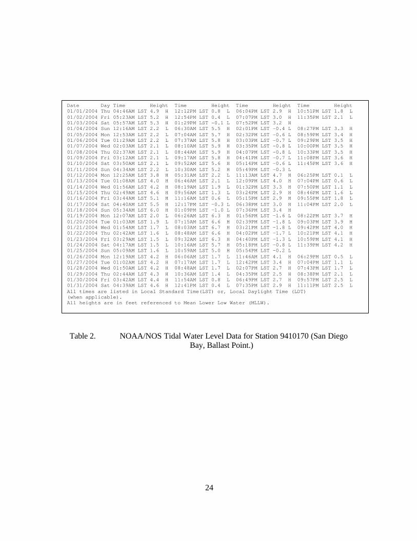
Table 2. NOAA/NOS Tidal Water Level Data for Station 9410170 (San Diego Bay, Ballast Point.)
Date Day Time Height Time Height Time Height Time Height 01/01/2004 Thu 04:46AM LST 4.9 H 12:12PM LST 0.8 L 06:04PM LST 2.9 H 10:51PM LST 1.8 L 01/02/2004 Fri 05:23AM LST 5.2 H 12:54PM LST 0.4 L 07:07PM LST 3.0 H 11:35PM LST 2.1 L 01/03/2004 Sat 05:57AM LST 5.3 H 01:29PM LST -0.1 L 07:52PM LST 3.2 H 01/04/2004 Sun 12:16AM LST 2.2 L 06:30AM LST 5.5 H 02:01PM LST -0.4 L 08:27PM LST 3.3 H 01/05/2004 Mon 12:53AM LST 2.2 L 07:04AM LST 5.7 H 02:32PM LST -0.6 L 08:59PM LST 3.4 H 01/06/2004 Tue 01:29AM LST 2.2 L 07:37AM LST 5.8 H 03:03PM LST -0.7 L 09:29PM LST 3.5 H 01/07/2004 Wed 02:03AM LST 2.1 L 08:10AM LST 5.9 H 03:35PM LST -0.8 L 10:00PM LST 3.5 H 01/08/2004 Thu 02:37AM LST 2.1 L 08:44AM LST 5.9 H 04:07PM LST -0.8 L 10:33PM LST 3.5 H 01/09/2004 Fri 03:12AM LST 2.1 L 09:17AM LST 5.8 H 04:41PM LST -0.7 L 11:08PM LST 3.6 H 01/10/2004 Sat 03:50AM LST 2.1 L 09:52AM LST 5.6 H 05:14PM LST -0.6 L 11:45PM LST 3.6 H 01/11/2004 Sun 04:34AM LST 2.2 L 10:30AM LST 5.2 H 05:49PM LST -0.3 L 01/12/2004 Mon 12:25AM LST 3.8 H 05:31AM LST 2.2 L 11:13AM LST 4.7 H 06:25PM LST 0.1 L 01/13/2004 Tue 01:08AM LST 4.0 H 06:46AM LST 2.1 L 12:09PM LST 4.0 H 07:04PM LST 0.6 L 01/14/2004 Wed 01:56AM LST 4.2 H 08:19AM LST 1.9 L 01:32PM LST 3.3 H 07:50PM LST 1.1 L 01/15/2004 Thu 02:49AM LST 4.6 H 09:56AM LST 1.3 L 03:24PM LST 2.9 H 08:46PM LST 1.6 L 01/16/2004 Fri 03:44AM LST 5.1 H 11:16AM LST 0.6 L 05:15PM LST 2.9 H 09:55PM LST 1.8 L 01/17/2004 Sat 04:40AM LST 5.5 H 12:17PM LST -0.3 L 06:38PM LST 3.0 H 11:04PM LST 2.0 L 01/18/2004 Sun 05:34AM LST 6.0 H 01:09PM LST -1.0 L 07:36PM LST 3.4 H 01/19/2004 Mon 12:07AM LST 2.0 L 06:26AM LST 6.3 H 01:56PM LST -1.6 L 08:22PM LST 3.7 H 01/20/2004 Tue 01:03AM LST 1.9 L 07:15AM LST 6.6 H 02:39PM LST -1.8 L 09:03PM LST 3.9 H 01/21/2004 Wed 01:54AM LST 1.7 L 08:03AM LST 6.7 H 03:21PM LST -1.8 L 09:42PM LST 4.0 H 01/22/2004 Thu 02:42AM LST 1.6 L 08:48AM LST 6.6 H 04:02PM LST -1.7 L 10:21PM LST 4.1 H 01/23/2004 Fri 03:29AM LST 1.5 L 09:32AM LST 6.3 H 04:40PM LST -1.3 L 10:59PM LST 4.1 H 01/24/2004 Sat 04:17AM LST 1.5 L 10:16AM LST 5.7 H 05:18PM LST -0.8 L 11:39PM LST 4.2 H 01/25/2004 Sun 05:09AM LST 1.6 L 10:59AM LST 5.0 H 05:54PM LST -0.2 L 01/26/2004 Mon 12:19AM LST 4.2 H 06:06AM LST 1.7 L 11:46AM LST 4.1 H 06:29PM LST 0.5 L 01/27/2004 Tue 01:02AM LST 4.2 H 07:17AM LST 1.7 L 12:42PM LST 3.4 H 07:04PM LST 1.1 L 01/28/2004 Wed 01:50AM LST 4.2 H 08:48AM LST 1.7 L 02:07PM LST 2.7 H 07:43PM LST 1.7 L 01/29/2004 Thu 02:44AM LST 4.3 H 10:36AM LST 1.4 L 04:35PM LST 2.5 H 08:38PM LST 2.1 L 01/30/2004 Fri 03:42AM LST 4.4 H 11:54AM LST 0.8 L 06:49PM LST 2.7 H 09:57PM LST 2.5 L 01/31/2004 Sat 04:39AM LST 4.6 H 12:41PM LST 0.4 L 07:35PM LST 2.9 H 11:11PM LST 2.5 L All times are listed in Local Standard Time(LST) or, Local Daylight Time (LDT) (when applicable). All heights are in feet referenced to Mean Lower Low Water (MLLW).

25
Table 3. NOAA/NOS Tidal Current Data for Station 9410170 (San Diego Bay, Ballast Point.).
San Diego Bay Entrance (off Ballast Point), California
Predicted Tidal Current January, 2004 Flood Direction, 355 True. Ebb (-)Direction, 175 True. NOAA, National Ocean Service Slack Maximum Slack Maximum Slack Maximum Slack Maximum Slack Water Current Water Current Water Current Water Current Water Day Time Time Veloc Time Time Veloc Time Time Veloc Time Time Veloc Time h.m. h.m. knots h.m. h.m. knots h.m. h.m. knots h.m. h.m. knots h.m.
1 236 1.1 533 858 -1.4 1302 1541 0.8 1821 2057 -0.7 2344 2 320 1.2 611 942 -1.7 1343 1630 1.0 1921 2147 -0.7 3 26 358 1.2 646 1020 -1.9 1418 1710 1.2 2010 2230 -0.8 4 102 432 1.3 719 1054 -2.1 1450 1747 1.3 2051 2308 -0.8 5 136 503 1.3 751 1128 -2.2 1520 1820 1.4 2128 2343 -0.8 6 207 531 1.3 822 1200 -2.3 1550 1851 1.4 2203 7 16 -0.8 237 558 1.3 852 1232 -2.3 1621 1921 1.4 2236 8 49 -0.8 306 624 1.3 922 1305 -2.3 1651 1951 1.4 2309 9 123 -0.8 339 653 1.3 953 1339 -2.3 1723 2021 1.3 2343 10 200 -0.8 416 725 1.2 1026 1415 -2.1 1756 2053 1.3 11 19 241 -0.8 501 804 1.1 1103 1454 -1.9 1830 2128 1.2 12 58 329 -0.8 559 851 0.9 1147 1539 -1.7 1908 2210 1.1 13 143 426 -0.9 714 954 0.7 1245 1632 -1.3 1951 2302 1.1 14 234 535 -1.0 853 1126 0.5 1409 1739 -1.0 2041 15 7 1.0 331 650 -1.2 1041 1326 0.6 1604 1858 -0.8 2141 16 119 1.1 430 802 -1.6 1204 1458 0.8 1749 2017 -0.7 2247 17 227 1.2 526 906 -2.0 1305 1604 1.2 1907 2126 -0.8 2351 18 326 1.4 620 1001 -2.4 1356 1657 1.5 2006 2224 -0.9 19 49 419 1.6 711 1051 -2.7 1442 1744 1.8 2055 2314 -1.1 20 140 507 1.8 759 1137 -2.9 1525 1827 1.9 2139 21 0 -1.2 228 552 1.9 845 1221 -3.0 1607 1908 2.0 2220 22 43 -1.2 314 635 1.8 929 1303 -2.9 1647 1948 1.9 2300 23 125 -1.3 400 716 1.7 1012 1343 -2.7 1724 2027 1.7 2338 24 208 -1.2 447 758 1.5 1053 1423 -2.3 1801 2105 1.5 25 18 252 -1.2 537 841 1.2 1134 1503 -1.9 1835 2143 1.3 26 58 339 -1.1 637 930 0.9 1218 1545 -1.5 1910 2225 1.1 27 143 433 -1.0 754 1034 0.5 1311 1633 -1.0 1947 2315 0.9 28 234 539 -0.9 946 1217 0.3 1432 1735 -0.6 2032 29 23 0.7 333 658 -1.0 1143 1412 0.4 1634 1859 -0.4 2136 30 143 0.7 434 815 -1.2 1248 1529 0.6 1819 2029 -0.4 2258 31 249 0.8 530 916 -1.4 1330 1621 0.9 1924 2136 -0.5
All times listed are in Local Time, and all speeds are in knots.
26
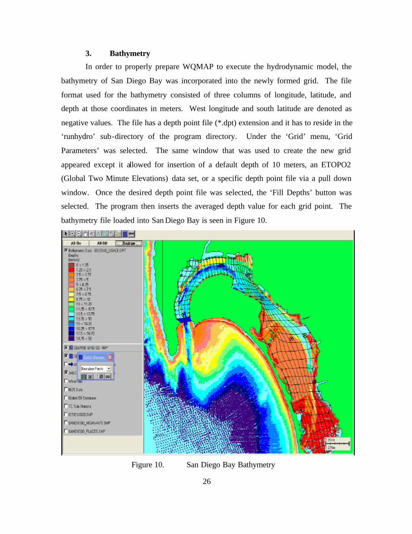
3. Bathymetry
In order to properly prepare WQMAP to execute the hydrodynamic model, the
bathymetry of San Diego Bay was incorporated into the newly formed grid. The file
format used for the bathymetry consisted of three columns of longitude, latitude, and
depth at those coordinates in meters. West longitude and south latitude are denoted as
negative values. The file has a depth point file (*.dpt) extension and it has to reside in the
‘runhydro’ sub-directory of the program directory. Under the ‘Grid’ menu, ‘Grid
Parameters’ was selected. The same window that was used to create the new grid
appeared except it allowed for insertion of a default depth of 10 meters, an ETOPO2
(Global Two Minute Elevations) data set, or a specific depth point file via a pull down
window. Once the desired depth point file was selected, the ‘Fill Depths’ button was
selected. The program then inserts the averaged depth value for each grid point. The
bathymetry file loaded into San Diego Bay is seen in Figure 10.
Figure 10. San Diego Bay Bathymetry
27
B. HYDRODYNAMIC MODEL EXECUTION
The program must have the desired forcing data file (*.hst) selected for the blue
open boundary cells as displayed in Figure 7. Under the ‘Data’ menu, ‘Select Cells by
Region’ is chosen, followed by sub-directory choice of ‘Boundary Cells’. The mouse
pointer turns into a cross symbol. A simple geometric shape is then drawn around the
blue open boundary cells. A separate window appears giving the operator the option of
selecting either ‘Tidal Constituents’ or ‘Time Series File’ choices. The selection of
‘Time Series File’ followed by the choice of the desired Open Boundary Tidal Forcing
File (*.hst) from a pull down window places the file time series contents for the forcing
elevation to the blue open boundary cells. With the boundary fitted grid designed; the
bathymetry is loaded into the grid. Finally the desired forcing data is then obtained,
formatted and assigned to the open boundary cells; then the hydrodynamic model is ready
for execution. Under the ‘Run Model’ menu, the ‘Hydrodynamic Model’ choice starts
the process. The separate window that opens has three separate option tabs, Model Run
Control, Model Parameters, and Physical Parameters.
1. Model Run Control
Within this section the run length of the model is determined. The start time and
end time are entered as date and time. The interval for the current time series and the
interval for current field output, each in minutes, are also specified here. Due to time
constraints, the program that allows for modeling using a file with a wind time series at
the surface boundary was not able to be utilized for this analysis. The run time for this
study began on 0000 January 1st, 2004 and ended on 2354 January 31st, 2004. Interval
for the current field time series and the interval for current field output were both set to
six minutes.
2. Model Parameters
Details specific to the modeling numerics are stipulated within this section.
Inputs by the user for number of Z grids (3-D only) as well as model time step, ramp time
period and residual start time in minutes are to be provided. The model can be run in a
baroclinic process with prognostic terms for salinity and temperature and the advection
time step in minutes can all be chosen. The hydrodynamic model as a baroclinic process
28
was not run in this study. The time step was set to six minutes and the ramp time period
and residual start time were set for one day (1,440 minutes).
3. Physical Parameters
All physical parameters that affect the hydrodynamic model are defined here.
This section requires wind drag coeffient, vertical viscosity (m2/sec), vertical dispersion
(m2/sec), horizontal dispersion (m2/sec), and the bottom drag coefficient to be specified.
If salinity and temperature advection are to be modeled, initial temperature in degrees
Celsius and initial salinity in parts per thousand (ppt) can be stipulated as well. This
study utilized the default values as follows: wind drag coefficient 0.0014, ve rtical
viscosity 0.005, vertical dispersion 0.001, and horizontal dispersion 1.0, and the bottom
drag coefficient 0.003.
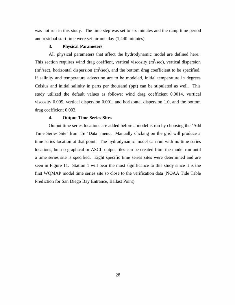
4. Output Time Series Sites
Output time series locations are added before a model is run by choosing the ‘Add
Time Series Site’ from the ‘Data’ menu. Manually clicking on the grid will produce a
time series location at that point. The hydrodynamic model can run with no time series
locations, but no graphical or ASCII output files can be created from the model run until
a time series site is specified. Eight specific time series sites were determined and are
seen in Figure 11. Station 1 will bear the most significance to this study since it is the
first WQMAP model time series site so close to the verification data (NOAA Tide Table
Prediction for San Diego Bay Entrance, Ballast Point).
29
Figure 11. Time Series Sites
30
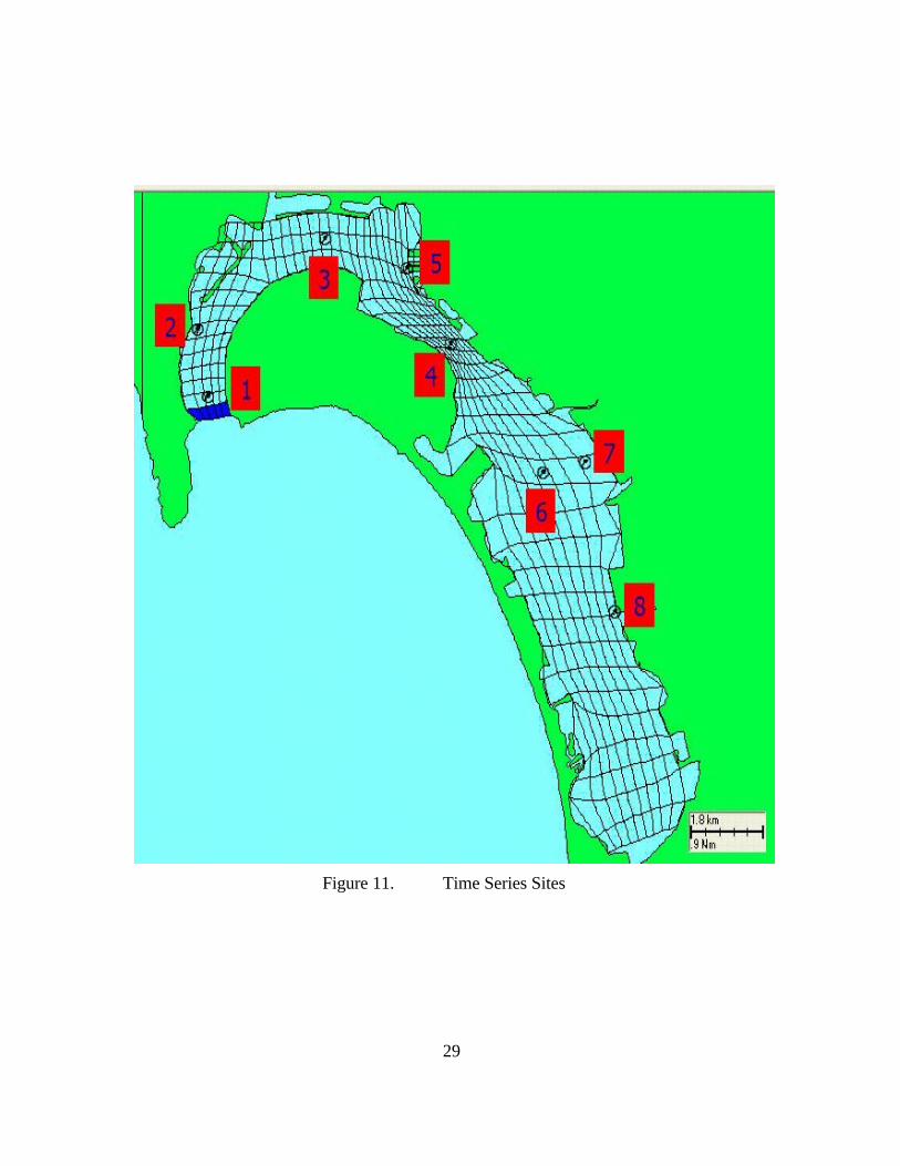
5. GUI Results
Once all model parameters and settings are provided, a click of the hydrodynamic
model button at the top of the window starts the process. The model calculates the
elevation, east-west velocity (u), and north-south velocity (v) for each grid point during
each time step. It then creates a new GIS layer for the modeled currents. With his layer
activated, the program can animate the modeled current speeds and directions with vector
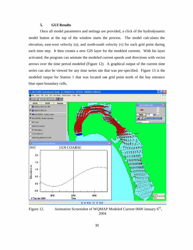
arrows over the time period modeled (Figure 12). A graphical output of the current time
series can also be viewed for any time series site that was pre-specified. Figure 13 is the
modeled output for Station 1 that was located one grid point north of the bay entrance
blue open boundary cells.
Figure 12. Animation Screenshot of WQMAP Modeled Current 0600 January 6th,
2004
31
Figure 13. Station 1 WQMAP Modeled Current January 2004
32
C. DATA PROCESSING
1. WQMAP Output Files
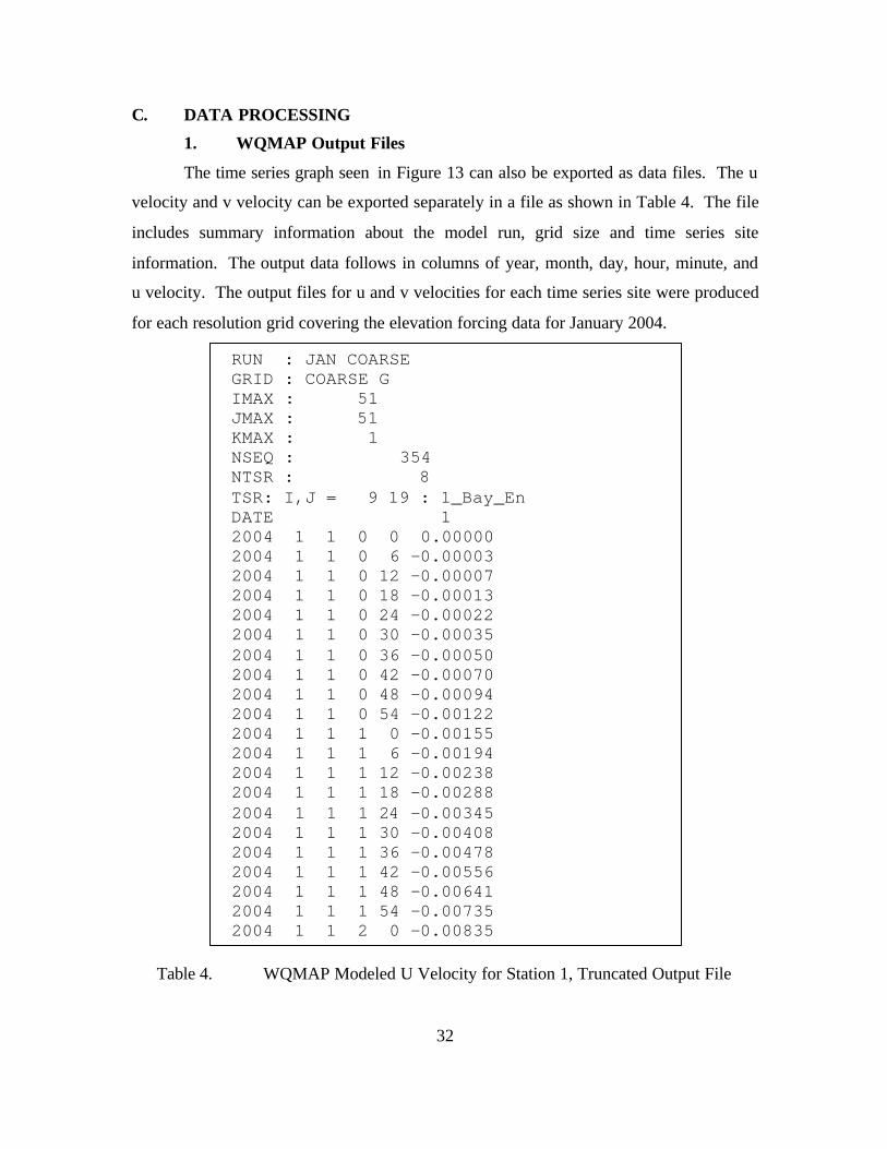
The time series graph seen in Figure 13 can also be exported as data files. The u
velocity and v velocity can be exported separately in a file as shown in Table 4. The file
includes summary information about the model run, grid size and time series site
information. The output data follows in columns of year, month, day, hour, minute, and
u velocity. The output files for u and v velocities for each time series site were produced
for each resolution grid covering the elevation forcing data for January 2004.
Table 4. WQMAP Modeled U Velocity for Station 1, Truncated Output File
RUN : JAN COARSE GRID : COARSE G IMAX : 51 JMAX : 51 KMAX : 1 NSEQ : 354 NTSR : 8 TSR: I,J = 9 19 : 1_Bay_En DATE 1 2004 1 1 0 0 0.00000 2004 1 1 0 6 -0.00003 2004 1 1 0 12 -0.00007 2004 1 1 0 18 -0.00013 2004 1 1 0 24 -0.00022 2004 1 1 0 30 -0.00035 2004 1 1 0 36 -0.00050 2004 1 1 0 42 -0.00070 2004 1 1 0 48 -0.00094 2004 1 1 0 54 -0.00122 2004 1 1 1 0 -0.00155 2004 1 1 1 6 -0.00194 2004 1 1 1 12 -0.00238 2004 1 1 1 18 -0.00288 2004 1 1 1 24 -0.00345 2004 1 1 1 30 -0.00408 2004 1 1 1 36 -0.00478 2004 1 1 1 42 -0.00556 2004 1 1 1 48 -0.00641 2004 1 1 1 54 -0.00735 2004 1 1 2 0 -0.00835
33
2. Rotational Matrix
WQMAP’s output for the u velocity is positive for the east direction and negative
for the west direction. Similarly, the v velocity is positive in the north direction and
negative in the south direction. The NOAA Tide Table data used to verify the
WQMAP’s model of Station 1 is in reference to a positive value for the flood direction of
355° True and a negative value for the ebb direction of 175° True. This orientation of
flood and ebb directions needs to be applied to the WQMAP u and v velocity output data
sets. Note that each time series site has a different flood and ebb direction than that of
Station 1. Different re-orientation calculations have to be made with each time series
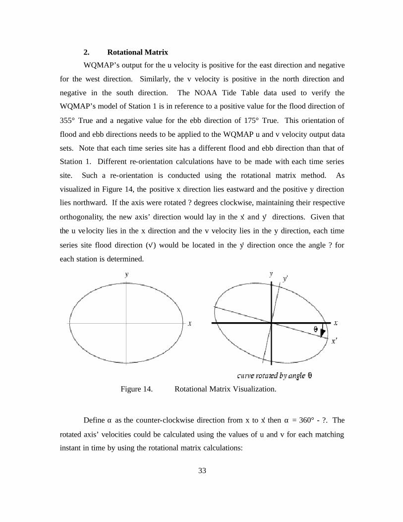
site. Such a re-orientation is conducted using the rotational matrix method. As
visualized in Figure 14, the positive x direction lies eastward and the positive y direction
lies northward. If the axis were rotated ? degrees clockwise, maintaining their respective
orthogonality, the new axis’ direction would lay in the x′ and y′ directions. Given that
the u velocity lies in the x direction and the v velocity lies in the y direction, each time
series site flood direction (v′) would be located in the y′ direction once the angle ? for
each station is determined.
Figure 14. Rotational Matrix Visualization.
Define α as the counter-clockwise direction from x to x′ then α = 360° - ?. The
rotated axis’ velocities could be calculated using the values of u and v for each matching
instant in time by using the rotational matrix calculations:
34
cos sinu u vα α′ = + (12)
cos sinv v uα α′ = − (13)
The resultant calculations provide positive values of v′ as a flood current and
negative values of v′ as an ebb current. Each time series of the site u and v output files
were summarily imported and the rotational matrix calculation for each station was
conducted after measuring the angle α at each station.
35
IV. RESULTS
A. DIFFERENCE BETWEEN DIFFERENT RESOLUTION GRIDS
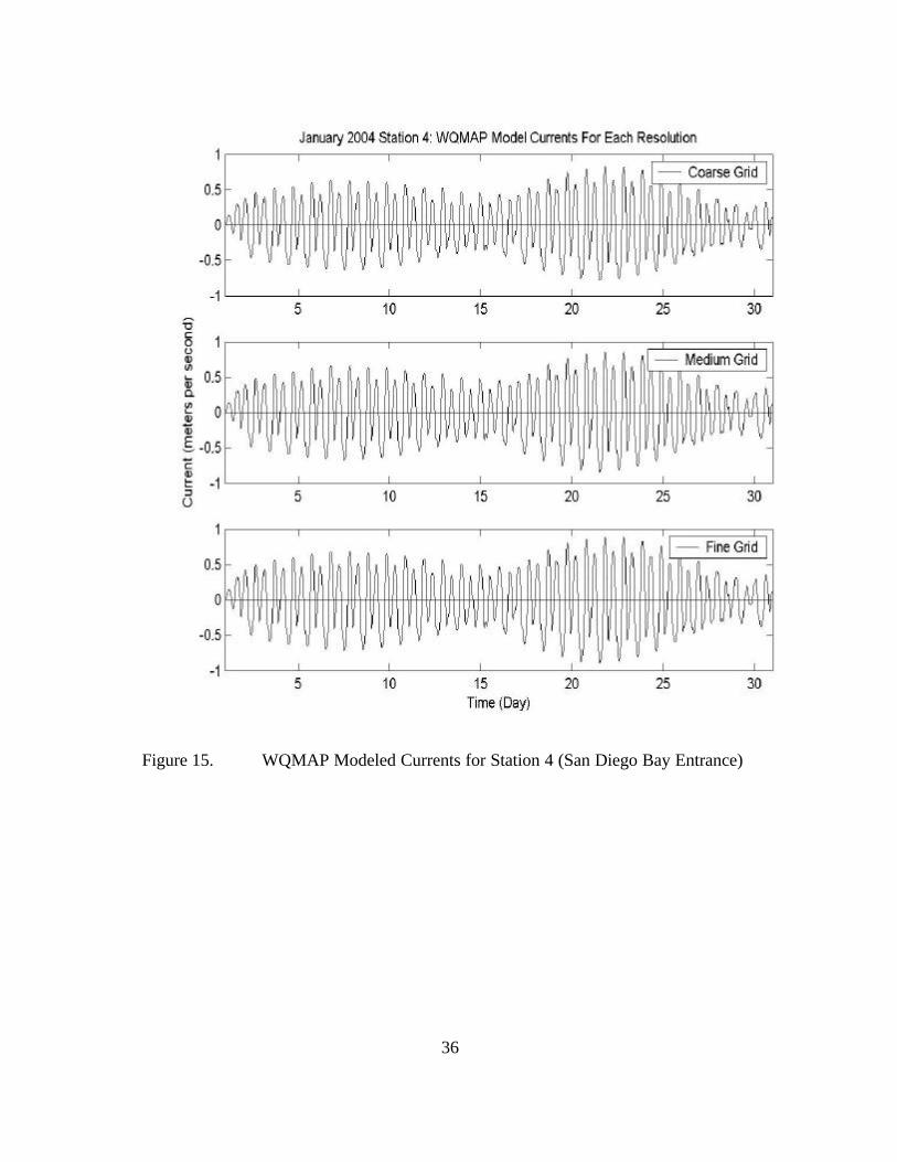
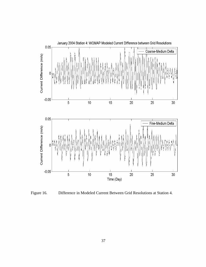
The WQMAP modeled current results for each grid resolution for Station 4 (San
Diego-Coronado Bridge) are displayed in Figure 15. The difference in the modeled
currents between each grid is so fine that a superposition plot of all three grid results
cannot be discerned visually. A plot of the difference between each resolution is
provided in Figure 16 where the medium grid modeled currents is used as a reference
between the other two grids. The maximum difference between the medium grid and the
coarse grid currents is 0.05 m/s. The maximum difference between the medium grid and
the fine grid currents is slightly less at 0.04 m/s. The medium to coarse grid current
difference has root mean square error of 0.0222 m/s whereas the fine to medium
difference in currents has a root mean square of 0.0164 m/s. Given these values of
maximum current differences as well as the root mean square error, the current prediction
is for any grid resolution selection correlates reasonably well. All future comparisons to
model output will be made with the fine resolution grid. Since it allows nearly the same
grid modeled output correlation while providing more grid cell time series site selections
for either future comparisons or operational planning needs.
36
Figure 15. WQMAP Modeled Currents for Station 4 (San Diego Bay Entrance)
37
Figure 16. Difference in Modeled Current Between Grid Resolutions at Station 4.
38
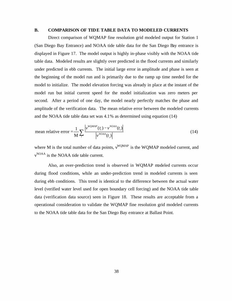
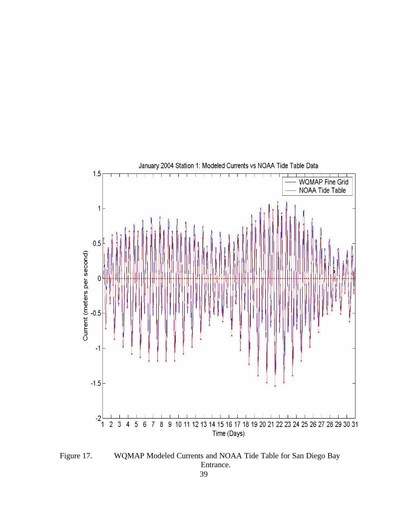
B. COMPARISON OF TIDE TABLE DATA TO MODELED CURRENTS
Direct comparison of WQMAP fine resolution grid modeled output for Station 1
(San Diego Bay Entrance) and NOAA tide table data for the San Diego Bay entrance is
displayed in Figure 17. The model output is highly in-phase visibly with the NOAA tide
table data. Modeled results are slightly over predicted in the flood currents and similarly
under predicted in ebb currents. The initial large error in amplitude and phase is seen at
the beginning of the model run and is primarily due to the ramp up time needed for the
model to initialize. The model elevation forcing was already in place at the instant of the
model run but initial current speed for the model initialization was zero meters per
second. After a period of one day, the model nearly perfectly matches the phase and
amplitude of the verification data. The mean relative error between the modeled currents
and the NOAA tide table data set was 4.1% as determined using equation (14)
( ) ( )1mean relative error =
M ( )
WQMAP NOAAi i
NOAAi i
v t v t
v t
−∑ (14)
where M is the total number of data points, vWQMAP is the WQMAP modeled current, and
vNOAA is the NOAA tide table current.
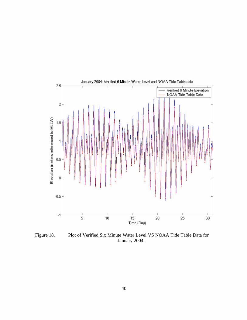
Also, an over-prediction trend is observed in WQMAP modeled currents occur
during flood conditions, while an under-prediction trend in modeled currents is seen
during ebb conditions. This trend is identical to the difference between the actual water
level (verified water level used for open boundary cell forcing) and the NOAA tide table
data (verification data source) seen in Figure 18. These results are acceptable from a
operational consideration to validate the WQMAP fine resolution grid modeled currents
to the NOAA tide table data for the San Diego Bay entrance at Ballast Point.
39
Figure 17. WQMAP Modeled Currents and NOAA Tide Table for San Diego Bay
Entrance.
40
Figure 18. Plot of Verified Six Minute Water Level VS NOAA Tide Table Data for
January 2004.
41
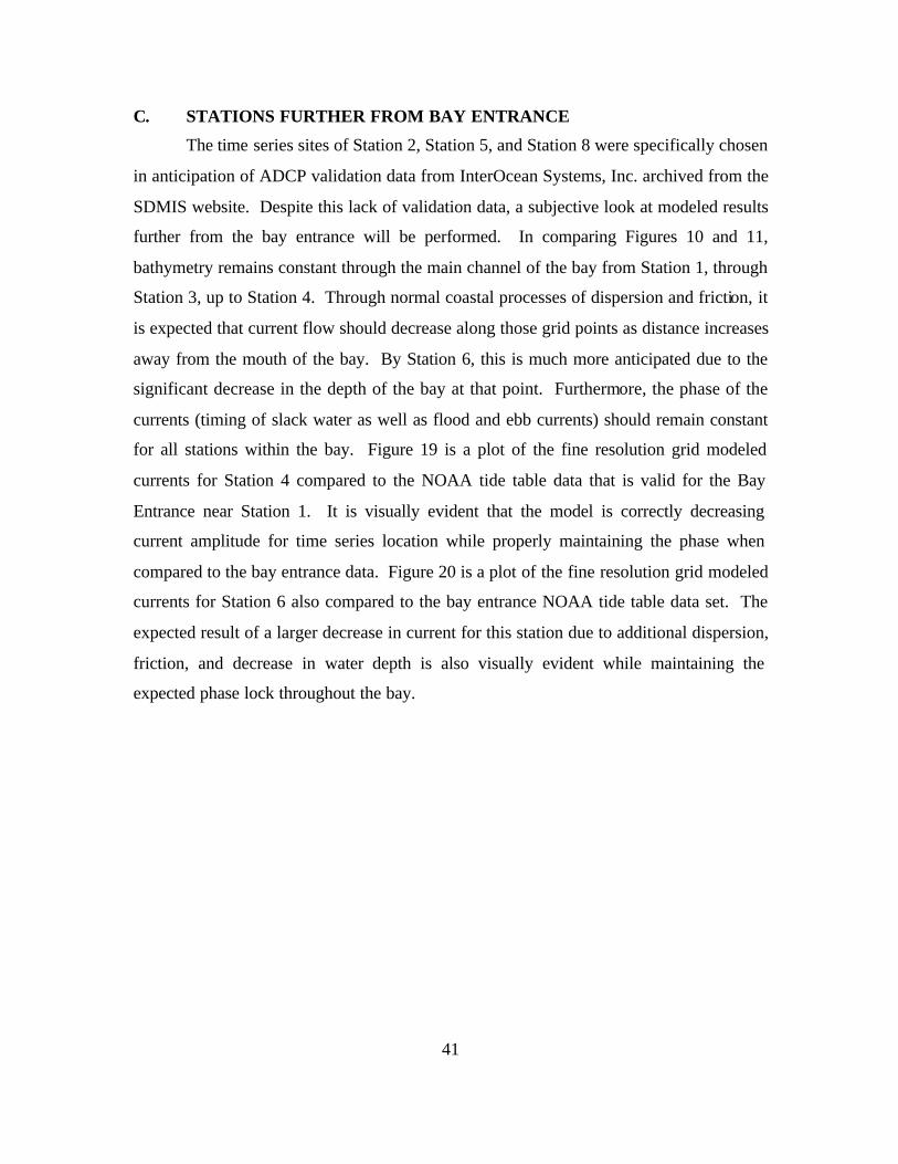
C. STATIONS FURTHER FROM BAY ENTRANCE
The time series sites of Station 2, Station 5, and Station 8 were specifically chosen
in anticipation of ADCP validation data from InterOcean Systems, Inc. archived from the
SDMIS website. Despite this lack of validation data, a subjective look at modeled results
further from the bay entrance will be performed. In comparing Figures 10 and 11,
bathymetry remains constant through the main channel of the bay from Station 1, through
Station 3, up to Station 4. Through normal coastal processes of dispersion and friction, it
is expected that current flow should decrease along those grid points as distance increases
away from the mouth of the bay. By Station 6, this is much more anticipated due to the
significant decrease in the depth of the bay at that point. Furthermore, the phase of the
currents (timing of slack water as well as flood and ebb currents) should remain constant
for all stations within the bay. Figure 19 is a plot of the fine resolution grid modeled
currents for Station 4 compared to the NOAA tide table data that is valid for the Bay
Entrance near Station 1. It is visually evident that the model is correctly decreasing
current amplitude for time series location while properly maintaining the phase when
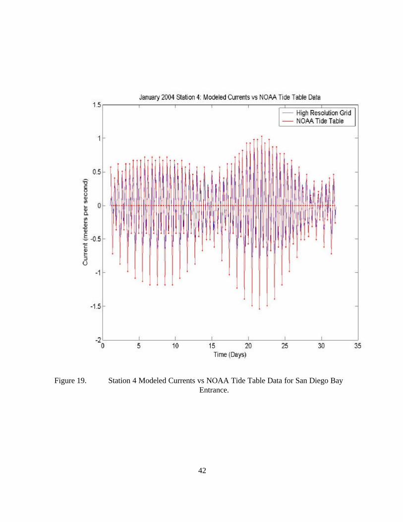
compared to the bay entrance data. Figure 20 is a plot of the fine resolution grid modeled
currents for Station 6 also compared to the bay entrance NOAA tide table data set. The
expected result of a larger decrease in current for this station due to additional dispersion,
friction, and decrease in water depth is also visually evident while maintaining the
expected phase lock throughout the bay.
42
Figure 19. Station 4 Modeled Currents vs NOAA Tide Table Data for San Diego Bay
Entrance.
43
Figure 20. Station 6 Modeled Currents vs NOAA Tide Table Data for San Diego Bay
Entrance.

44
THIS PAGE INTENTIONALLY LEFT BLANK
45
V. CONCLUSIONS
A. NEED FOR ADCP DATA
Despite that Station 1 had a relative error of 4.11% validates the model well for
operational considerations; determining the relative error for other stations within the bay
is in order to attest the effectiveness of this study. The validation of this model is
imperfect without proper real time observed current results from an ADCP. Despite the
strong correlation Station 1 had to the NOAA tide table data, real time data for Station 1
is necessary to assess the model’s true correlation to verified results at the same location.
Proper time series analysis for coherence and phase comparison to the NOAA tide tables
cannot be conducted given the varying time step of the tide table data. Consistent real
time data of current with a constant time step will be able to provide such an analysis.
WQMAP permits the user to self define the time step interval for the model and for the
output time series itself. Whatever ADCP data time step that may be available or
obtained can be matched by the hydrodynamic model within the ‘Model Run Control’
initial settings. Furthermore, validation for any other station or time series site cannot be
conducted at all without such validation data. An additional study should be planned and
conducted utilizing the boundary fitted grids created within this model using coordinated
matching forcing data from the NOAA CO-OPS verified elevation data portal and
verification data obtained by placing additional ADCPs at key stations of interest with
San Diego Bay.
B. APPLICATION OF MODELED RESULTS
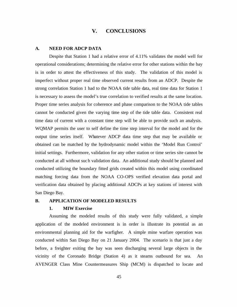
1. MIW Exercise
Assuming the modeled results of this study were fully validated, a simple
application of the modeled environment is in order is illustrate its potential as an
environmental planning aid for the warfigher. A simple mine warfare operation was
conducted within San Diego Bay on 21 January 2004. The scenario is that just a day
before, a freighter exiting the bay was seen discharging several large objects in the
vicinity of the Coronado Bridge (Station 4) as it steams outbound for sea. An
AVENGER Class Mine Countermeasures Ship (MCM) is dispatched to locate and

46
identify the mine like objects utilizing its AN/SQQ-32 Variable Depth Minehunting
Sonar along with the AN/SLQ-48 Mine Neutralization Vehicle (MNV). The current
thresholds for these assets are operationally sensitive, so a fictitious and current limit of 2
knots will be used as an operational current threshold in this example. Figure 21
illustrates what the operational windows are, marked in green, given the threshold limits
to the MCM, marked in red, using the NOAA Tide Table data set. The MCM can operate
within this threshold all morning until 1110. Minehunting operations would be able to
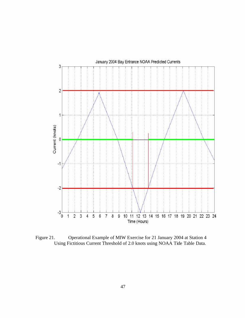
resume again around 1345 with no other restrictions for the rest of the day. Compare this
scenario with the modeled output from WQMAP for Station 4 for the same day (Figure
22). There is no timeframe that restricts minehunting operations us ing the WQMAP
modeled data set since the predicted currents do not exceed the operational threshold for
that location.
47
Figure 21. Operational Example of MIW Exercise for 21 January 2004 at Station 4
Using Fictitious Current Threshold of 2.0 knots using NOAA Tide Table Data.
48
Figure 22. Operational Example of MIW Exercise for 21 January 2004 at Station 4
Using Fictitious Current Threshold of 2.0 knots using WQMAP Fine Resolution Grid Modeled Currents.
49
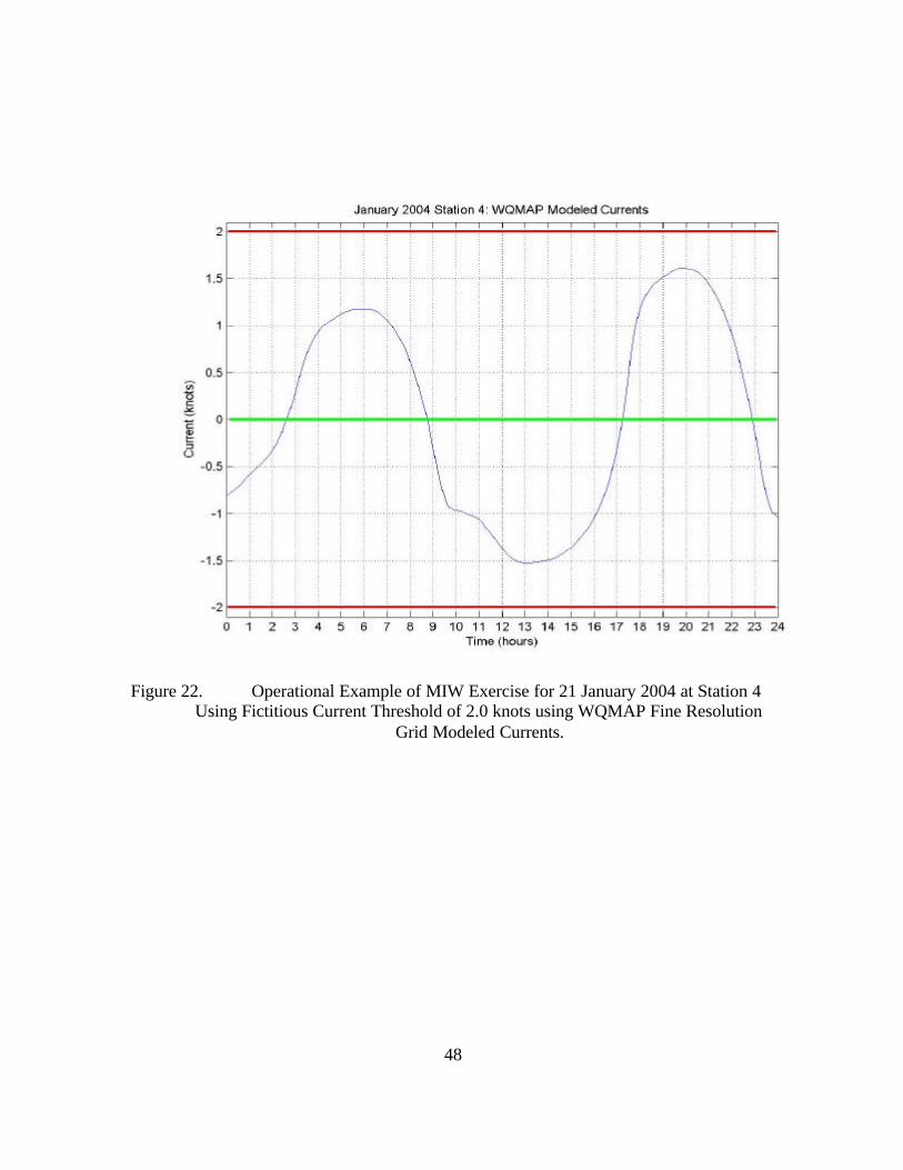
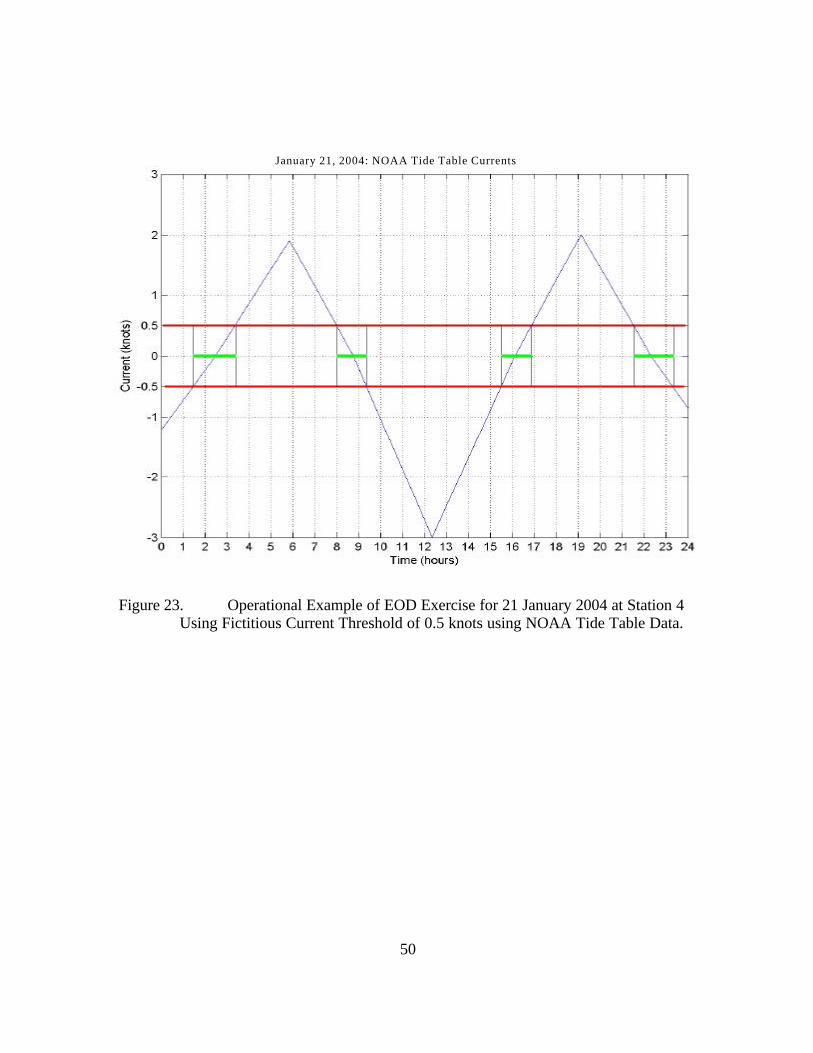
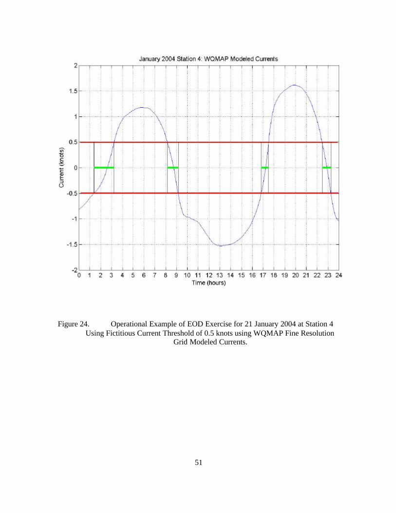
2. EOD Operation
An additional and more useful example is to extend the same operation on the
same day to include diving operations. One option to mine neutralization is to recover
the mine using an Explosive Ordnance Disposal (EOD) team. The scenario continues
with the MCM finding and identifying a mine like object as an actual mine. The mine
was found near a structural pylon of the Coronado Bridge so detonating it using the MNV
is not a desirable option. An EOD team is dispatched to retrieve the mine. Their
operational threshold for currents is also operationally sensitive so a fictitious limit of 0.5
knots will be used for this example. There are four operational windows for diving
operations in this scenario using the NOAA Tide Table data set (Figure 23). They range
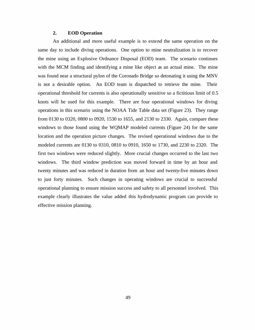
from 0130 to 0320, 0800 to 0920, 1530 to 1655, and 2130 to 2330. Again, compare these
windows to those found using the WQMAP modeled currents (Figure 24) for the same
location and the operation picture changes. The revised operational windows due to the
modeled currents are 0130 to 0310, 0810 to 0910, 1650 to 1730, and 2230 to 2320. The
first two windows were reduced slightly. More crucial changes occurred to the last two
windows. The third window prediction was moved forward in time by an hour and
twenty minutes and was reduced in duration from an hour and twenty-five minutes down
to just forty minutes. Such changes in operating windows are crucial to successful
operational planning to ensure mission success and safety to all personnel involved. This
example clearly illustrates the value added this hydrodynamic program can provide to
effective mission planning.
50
January 21, 2004: NOAA Tide Table Currents
Figure 23. Operational Example of EOD Exercise for 21 January 2004 at Station 4
Using Fictitious Current Threshold of 0.5 knots using NOAA Tide Table Data.
51
Figure 24. Operational Example of EOD Exercise for 21 January 2004 at Station 4 Using Fictitious Current Threshold of 0.5 knots using WQMAP Fine Resolution
Grid Modeled Currents.

52
C. FUTURE APPLICATION USING FLEET SURVEY TEAM ASSETS
As the warfare communities continue to advance in the realm of littoral warfare,
so will the support for those communities. There continues to be an increasing demand to
better model the much more complex coastal environment. WQMAP boundary fitted
grids can be developed for any coastal region, bay, or estuary. The current use of the
Naval Oceanographic Office’s Fleet Survey Teams (FST) can readily provide what is
needed to validate these models for each littoral grid that may be needed. The primary
mission of the FST is to obtain bathymetric data for navigational chart development.
This same bathymetry can by imported into a boundary fitted grid of the same region to
help model this environment. The FST can facilitate a successful model validation for a
coastal area of interest by obtaining elevation data during a survey period to be used as
forcing data for the open boundary cells defined within the model. Lastly, the FST, by
adding an ADCP to their inventory, can obtain verification data during their time frame
of their hydrographic survey. With proper planning, this NAVOCEANO asset can be
providing the warfare communities more than just an improved navigational product.
The FST’s mission in conjunction with the Naval Oceanographic Office’s Modeling and
Forecasting Divisions will be able to produce a series of small, PC-based current
prediction models that will be an invaluable benefit to future and unpredictable Naval
operations.
53
LIST OF REFERENCES
Arakawa, A. and Lamb, V. R., Computational Design of the Basic Dynamical Processes
of the UCLA General Circulation Model. Method in Computational Physics, v. 17, pp.
173-165, 1977.
Chadwick, D.B. and Largier, J.L., Tidal Exchange at the Bay-Ocean Boundary. Journal
of Geophysical Research, v. 104, no C12, pp. 29,901-29,924, 1999.
Chadwick, D.B. and Largier, J.L., The Influence of Tidal Range on the Exchange
Between San Diego Bay and the Ocean. Journal of Geophysical Research, v. 104, no.
C12, pp. 29,885-29,899, 1999.
Kantha, L, H and Clayson, C. A., Numerical Models of Ocean and Oceanic Processes,
Academic Press, San Diego, CA, pp. 940, 2000.
Muin, M. and M. L. Spaulding, Two-Dimensional Boundary Fitted Circulation Model in
Spherical Coordinates. Journal of Hydraulic Engineering, v. 122, no. 9, pp. 512-520,
1996.
Ritcher, K.; Sutton, D.; Reidy, L.; and Cheng, R, Comparison of Water Velocity Field
Data and Model Predictions in San Diego Bay. Oceans’95: Challenges of our Changing
Global Environment, v. 3, pp. 1751-1755, 1995.

54
THIS PAGE INTENTIONALLY LEFT BLANK

55
INITIAL DISTRIBUTION LIST
1. Defense Technical Information Center Ft. Belvoir, VA
2. Dudley Knox Library Naval Postgraduate School Monterey, CA
3. Mary L. Batteen Department of Oceanography Naval Postgraduate School Monterey, CA
4. Oceanographer of the Navy Naval Observatory Washington, D.C.
5. Commander Naval Meteorological and Oceanography Command Stennis Space Center, MS
6. Commanding Officer Naval Oceanographic Office Stennis Space Center, MS
7. Chief of Naval Research 800 North Quincy Street Arlington, VA
8. Superintendent Division 7300 - Oceanography Naval Research Laboratory Stennis Space Center, MS
9. Professor Peter C. Chu Code OC/CU
Department of Oceanography Naval Postgraduate School Monterey, CA
10. Mr. Edward C. Gough Jr Commander
Naval Meteorological and Oceanography Command Stennis Space Center, MS

56
11. CDR Eric Gottshall SPAWAR, PMW-155 12. Mr. Steve D. Haeger
Naval Oceanographic Office Stennis Space Center, MS
13. Dr. Edward Johnson Naval Oceanographic Office Stennis Space Center, MS
14. CDR Eric Long Chief of Naval Operations, N752 Washington, D.C.
15. Mr. Mark Null Naval Oceanographic Office Stennis Space Center, MS
16. Mr. Ron Betsch
Naval Oceanographic Office Stennis Space Center, MS
17. LT Albert E. Armstrong Naval Oceanographic Office Stennis Space Center, MS
Recommended