1/16
Prediction of Federal Funds Target Rate:A Dynamic Logistic Bayesian Model Averaging Approach
Hernán Alzate, MA, PhD-Student | [email protected]
Prof. Andrés Ramírez-Hassan, PhD| [email protected]
I Network de MÉTODOS CUANTITATIVOS EN ECONOMÍA

AGENDA
1. Introduction
2. Methodology & Simulation Exercises
3. Data & target rate characteristics
4. Empirical results: Estimation & Forecasting
5. Conclusions
6. Future research endeavors
2/16
3/16
Our goal is to identify which macroeconomic and financial variables are most informative for the Central Bank’s target rate decisions, by focusing particularly on the predictive power of Forward Rate Agreements: FRAsderived from the short-end of the Overnight-Indexed Swap curve: the OIS curve.
We used dynamic logistic models with dynamic Bayesian Model Averaging: BMA in order to perform predictions in real-time with more flexibility.
The computational burden of the algorithm is reduced by adapting a Markov Chain Monte Carlo Model Composition: MC3.
1. INTRODUCTION: MOTIVATION
1. INTRODUCTION: LITERATURE REVIEW
4/16
Krueger and Kuttner (1996), Söderström (1999) and Gürkaynak, R. (2005)
conclude that predictable changes in the fed funds rate are rationally
forecasted by the futures market; and a result, seems to be useful as a measure
of market and policy expectations.
Estrella and Hardouvelis (1991), Estrella and Mishkin (1998), Stock and Watson
(2000), Ang and Piazzesi (2003), and Diebold et al (2006), find strong evidence
of macroeconomic effects on the future yield curve.
In a recent study, Crump et al (2014) present evidence about how the path of
the policy rate constructed from fed funds futures, OIS, and Eurodollar futures
are useful tools to analyze market expectations.
S. van den Hauwe et al (2013), develop a Bayesian framework to model the
direction of FOMC target rate decisions.
2. METHODOLOGY
5/16
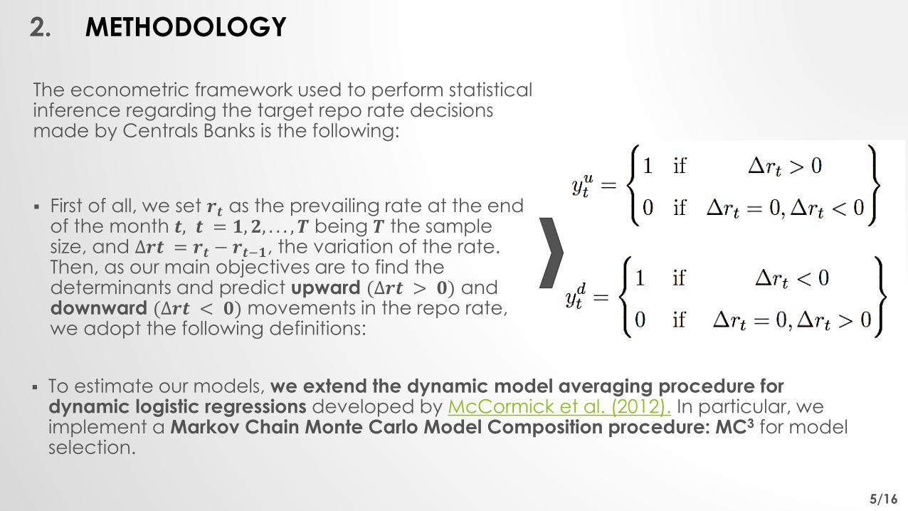
The econometric framework used to perform statistical inference regarding the target repo rate decisions made by Centrals Banks is the following:
First of all, we set 𝒓𝒕 as the prevailing rate at the end of the month 𝒕, 𝒕 = 𝟏, 𝟐, . . . , 𝑻 being 𝑻 the sample size, and ∆𝒓𝒕 = 𝒓𝒕 − 𝒓𝒕−𝟏, the variation of the rate. Then, as our main objectives are to find the determinants and predict upward (∆𝒓𝒕 > 𝟎) and downward (∆𝒓𝒕 < 𝟎) movements in the repo rate, we adopt the following definitions:
To estimate our models, we extend the dynamic model averaging procedure fordynamic logistic regressions developed by McCormick et al. (2012). In particular, weimplement a Markov Chain Monte Carlo Model Composition procedure: MC3 for modelselection.
2. METHODOLOGY (CONT.)
6/16
In particular, we initially build a design matrix 𝐗𝐽×𝐾, selecting predictors using a Bernoulli distribution with probability 𝒑. Such that each row of 𝐗 defines a candidate model, and our goal is to find the 𝐽 best models.
We calculate the average posterior model probability for these initial models,
𝜋 𝑀𝑇(𝑘)| 𝑦1:𝑇
𝐴𝑣𝑒= 1/𝑇 ∑ 𝑡=1
𝑇 𝜋 𝑀𝑡(𝑘)| 𝑦1:𝑡 , and find the model that has the minimum
posterior model probability, 𝑴𝒕(𝑴𝒊𝒏)
. Then, a candidate model 𝑴𝒕(𝒄)
is drawn randomly from the set of all models excluding the initial models, and we estimate its posterior model probability.
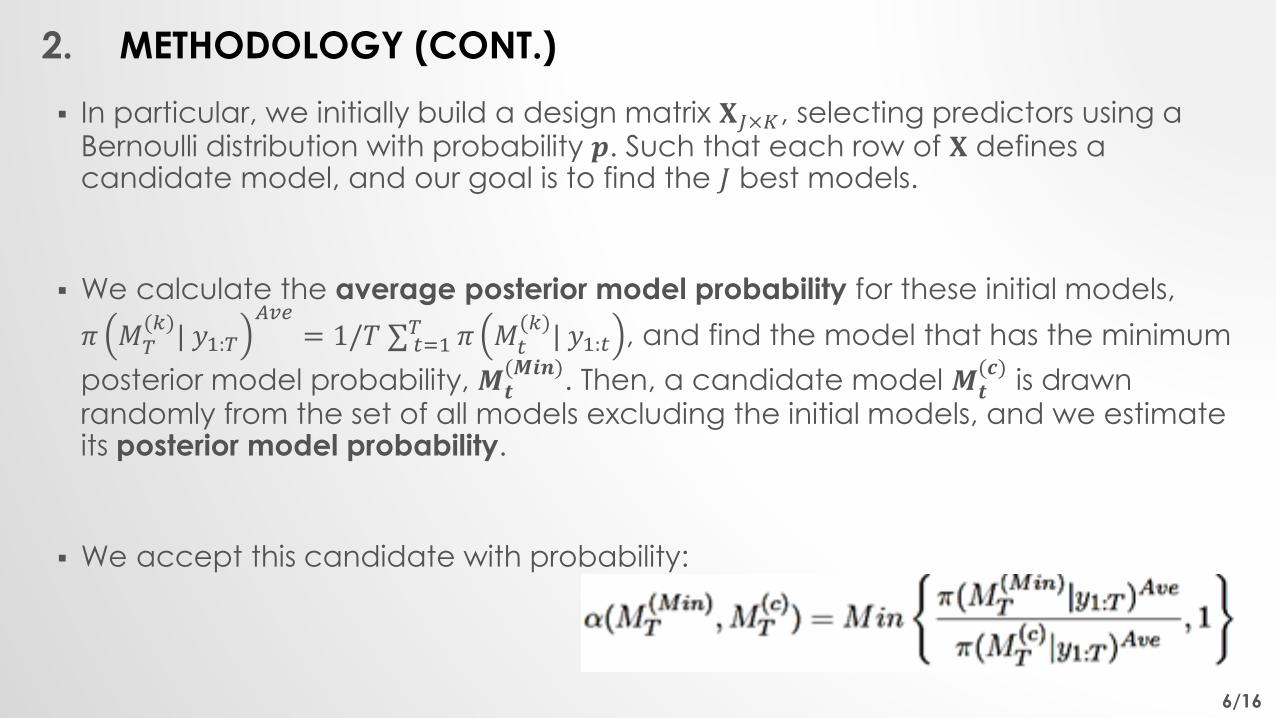
We accept this candidate with probability:
2. SIMULATION EXERCISES
7/16
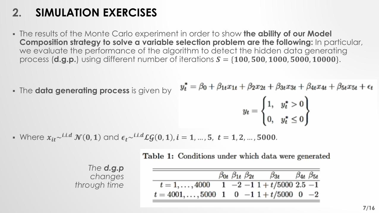
The results of the Monte Carlo experiment in order to show the ability of our Model Composition strategy to solve a variable selection problem are the following: In particular, we evaluate the performance of the algorithm to detect the hidden data generating process (d.g.p.) using different number of iterations 𝑺 = {𝟏𝟎𝟎, 𝟓𝟎𝟎, 𝟏𝟎𝟎𝟎, 𝟓𝟎𝟎𝟎, 𝟏𝟎𝟎𝟎𝟎}.
The data generating process is given by
Where 𝒙𝒊𝒕~𝒊.𝒊.𝒅𝓝 𝟎, 𝟏 and 𝝐𝒕~
𝒊.𝒊.𝒅𝓛𝓖 𝟎, 𝟏 , 𝒊 = 𝟏, … , 𝟓, 𝒕 = 𝟏, 𝟐, … , 𝟓𝟎𝟎𝟎.
The d.g.pchanges
through time
2. SIMULATION EXERCISES (CONT.)
8/16
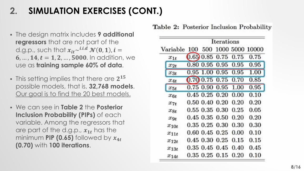
The design matrix includes 9 additional regressors that are not part of the
d.g.p., such that 𝒙𝒊𝒕~𝒊.𝒊.𝒅 𝓝 𝟎, 𝟏 , 𝒊 =
𝟔,… , 𝟏𝟒, 𝒕 = 𝟏, 𝟐, … , 𝟓𝟎𝟎𝟎. In addition, we
use as training sample 60% of data.
This setting implies that there are 𝟐𝟏𝟓
possible models, that is, 32,768 models.
Our goal is to find the 20 best models.
We can see in Table 2 the Posterior
Inclusion Probability (PIPs) of each
variable. Among the regressors that
are part of the d.g.p., 𝒙𝟏𝒕 has the minimum PIP (0.65) followed by 𝒙𝟒𝒕(0.70) with 100 iterations.
3. DATA & TARGET RATE CHARACTERISTICS
9/16
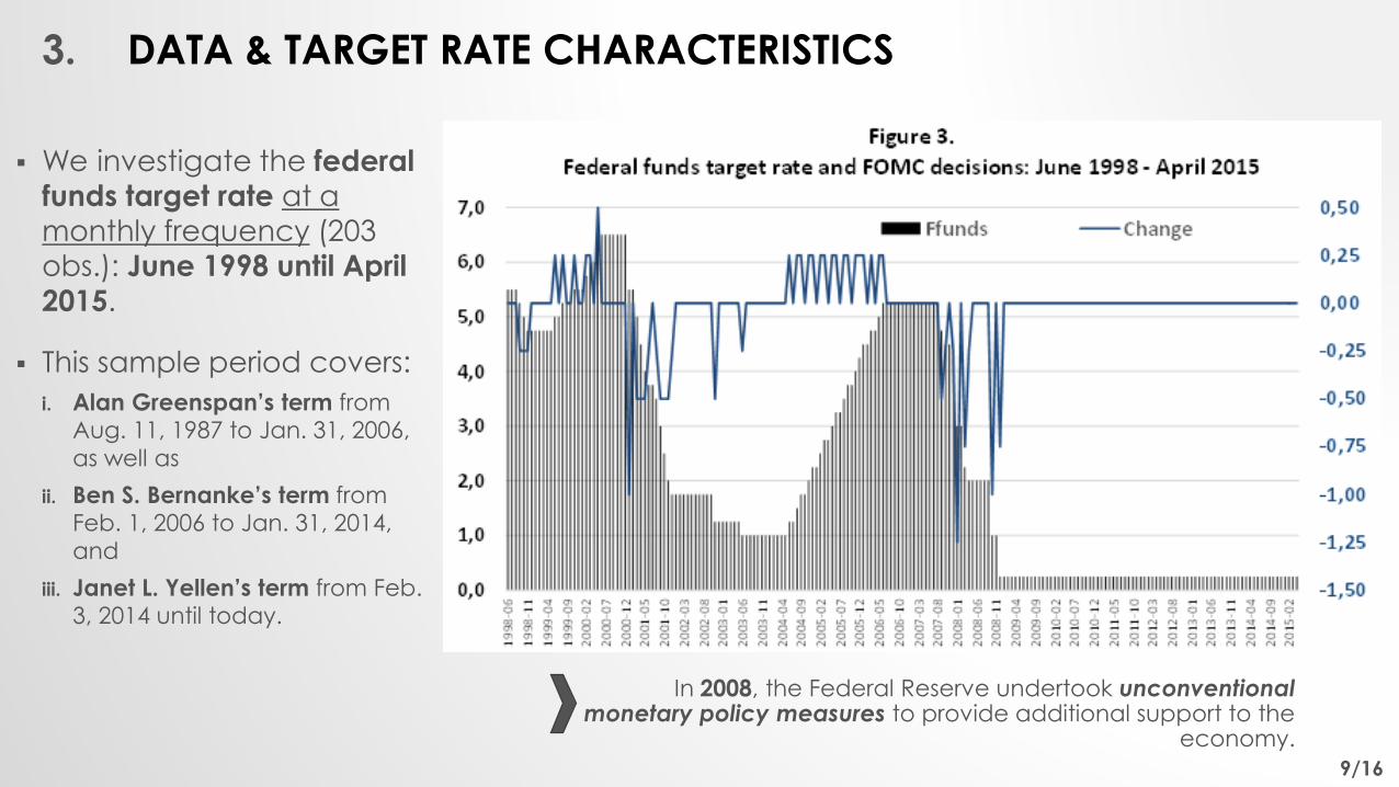
We investigate the federal
funds target rate at a
monthly frequency (203
obs.): June 1998 until April
2015.
This sample period covers:
i. Alan Greenspan’s term from Aug. 11, 1987 to Jan. 31, 2006,
as well as
ii. Ben S. Bernanke’s term from Feb. 1, 2006 to Jan. 31, 2014,
and
iii. Janet L. Yellen’s term from Feb. 3, 2014 until today.
In 2008, the Federal Reserve undertook unconventional monetary policy measures to provide additional support to the
economy.
3. DATA & TARGET RATE CHARACTERISTICS (CONT.)
10/16
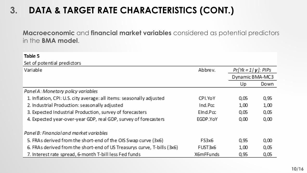
Macroeconomic and financial market variables considered as potential predictors
in the BMA model.
4. EMPIRICAL RESULTS: ESTIMATION
11/16
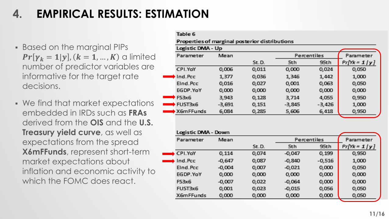
Based on the marginal PIPs
𝑷𝒓 𝜸𝒌 = 𝟏|𝒚 , 𝒌 = 𝟏,… ,𝑲 a limited
number of predictor variables are informative for the target rate
decisions.
We find that market expectations
embedded in IRDs such as FRAs
derived from the OIS and the U.S.
Treasury yield curve, as well as
expectations from the spread
X6mFFunds, represent short-term
market expectations about
inflation and economic activity to
which the FOMC does react.
4. EMPIRICAL RESULTS: FORECASTING
12/16
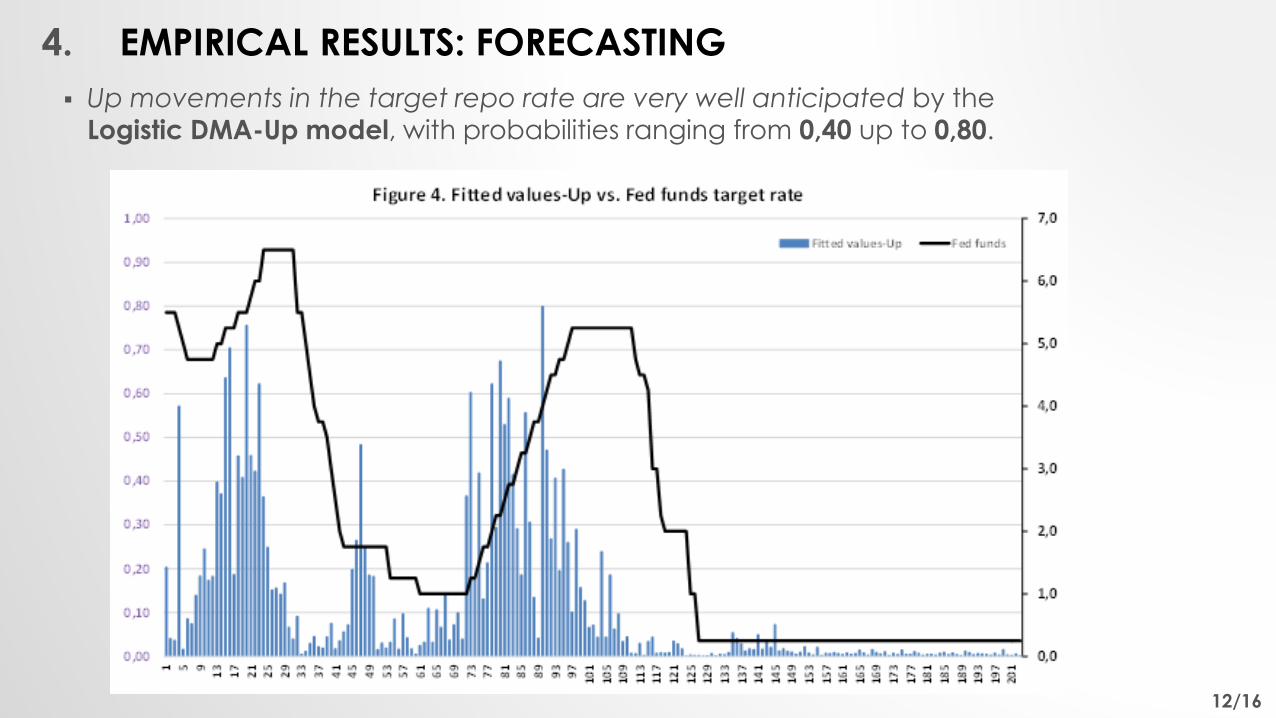
Up movements in the target repo rate are very well anticipated by the
Logistic DMA-Up model, with probabilities ranging from 0,40 up to 0,80.
13/16
0.0
1.0
2.0
3.0
4.0
5.0
6.0
7.0
0.00
0.10
0.20
0.30
0.40
0.50
0.60
0.70
0.80
0.90
1.00
19
98
-07
19
98
-11
19
99
-03
19
99
-07
19
99
-11
20
00
-03
20
00
-07
20
00
-11
20
01
-03
20
01
-07
20
01
-11
20
02
-03
20
02
-07
20
02
-11
20
03
-03
20
03
-07
20
03
-11
20
04
-03
20
04
-07
20
04
-11
20
05
-03
20
05
-07
20
05
-11
20
06
-03
20
06
-07
20
06
-11
20
07
-03
20
07
-07
20
07
-11
20
08
-03
20
08
-07
20
08
-11
20
09
-03
20
09
-07
20
09
-11
20
10
-03
20
10
-07
20
10
-11
20
11
-03
20
11
-07
20
11
-11
20
12
-03
20
12
-07
20
12
-11
20
13
-03
20
13
-07
20
13
-11
20
14
-03
20
14
-07
20
14
-11
20
15
-03
20
15
-07
20
15
-11
20
16
-04
20
16
-10
20
17
-02
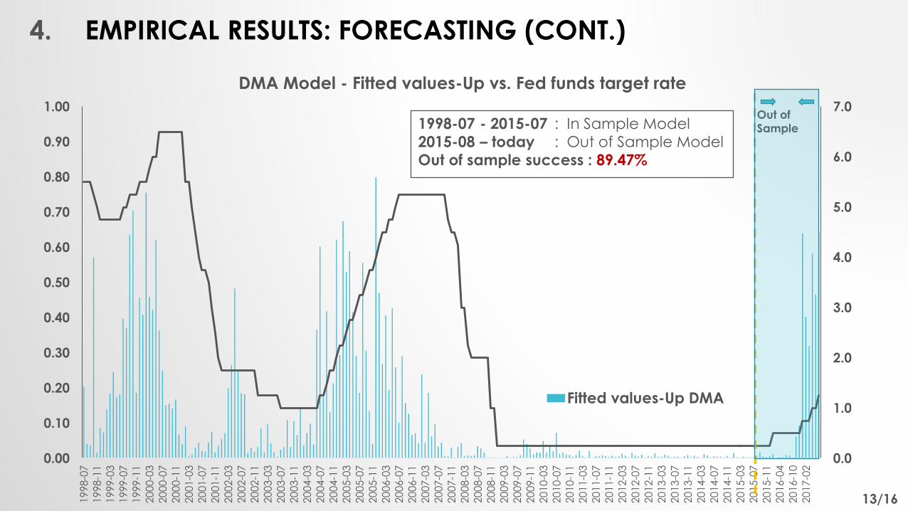
DMA Model - Fitted values-Up vs. Fed funds target rate
Fitted values-Up DMA
1998-07 - 2015-07 : In Sample Model
2015-08 – today : Out of Sample Model
Out of sample success : 89.47%
Out of
Sample
4. EMPIRICAL RESULTS: FORECASTING (CONT.)
5. CONCLUSIONS
14/16
i. Methodology:The analysis of FOMC’s decisions using dynamic logistic models with dynamicBayesian Model Averaging: BMA allows to perform predictions in real-time withgreat flexibility. In addition, by adapting a MC3 procedure the computationalburden of the algorithm was reduced efficiently.
ii. Empirical results:
For the Logistic DMA-Up model, the most predictive ability is found for: (i) economic
activity measures like Industrial Production; and (ii) term structure variables such as:
3x6 FRAs derived from the OIS curve and the USTY curve, as well as interest rate
spreads: X6mFFunds. Nonetheless, for the Logistic DMA-Down, the most predictive
ability rests on macro variables such as Industrial Production and y/y CPI.
6. FUTURE RESEARCH ENDEAVORS
15/16
The following ideas could be explored in order to improve the results and the methodology presented in this paper:
i. Design and algorithm that takes into account the trinomial case (multinomial classification),
where the three (3) possible states of the FOMC decisions could be very well captured.
ii. Perform ‘pattern net’ analysis associated with neural networks classification and compare
the results with the output provided by our model: the Bayes classification approach.
iii. Conduct this analysis for the Economic and Monetary Union (EMU) and contrast the results by running out-of-sample estimates in order to stress the model and test its predictive power
throughout the sample period.
iv. …among others.
16/16
Prediction of Federal Funds Target Rate:A Dynamic Logistic Bayesian Model Averaging Approach
Hernán Alzate, MA, PhD-Student | [email protected]
Prof. Andrés Ramírez-Hassan, PhD| [email protected]
Recommended