1/39
Practical Classical Methods
2/39
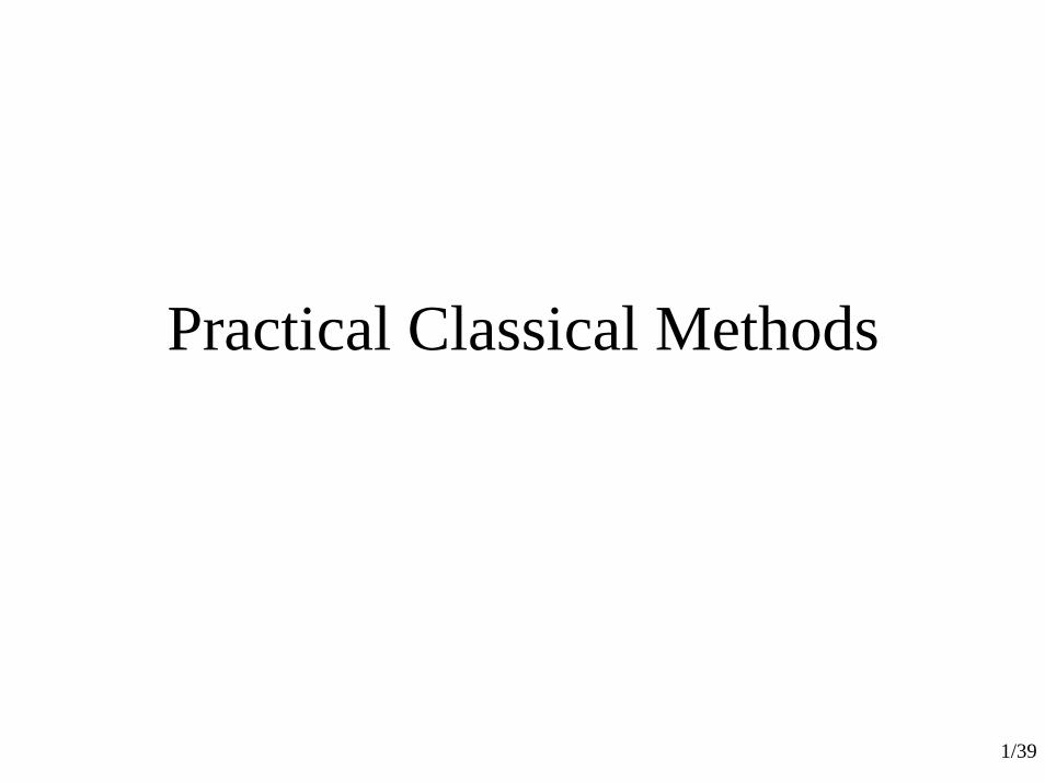
Main Problems of the Periodogram1. Biased Estimate2. Variance does NOT decrease with increasing N3. Rapid Fluctuations
All of these arise due to the fact that the periodogram ignores:• The Expected Value – (It includes no averaging)• The Limit Operation – (It applies a rectangular window)
in the PSD definition.
Several “classical” methods for partially fixing these have been proposed.
3/39
Modifications Based OnPeriodogram View
• Modified Periodogram• Bartlett Method• Welch Method
4/39
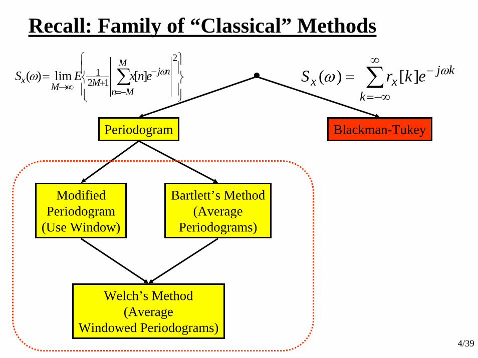
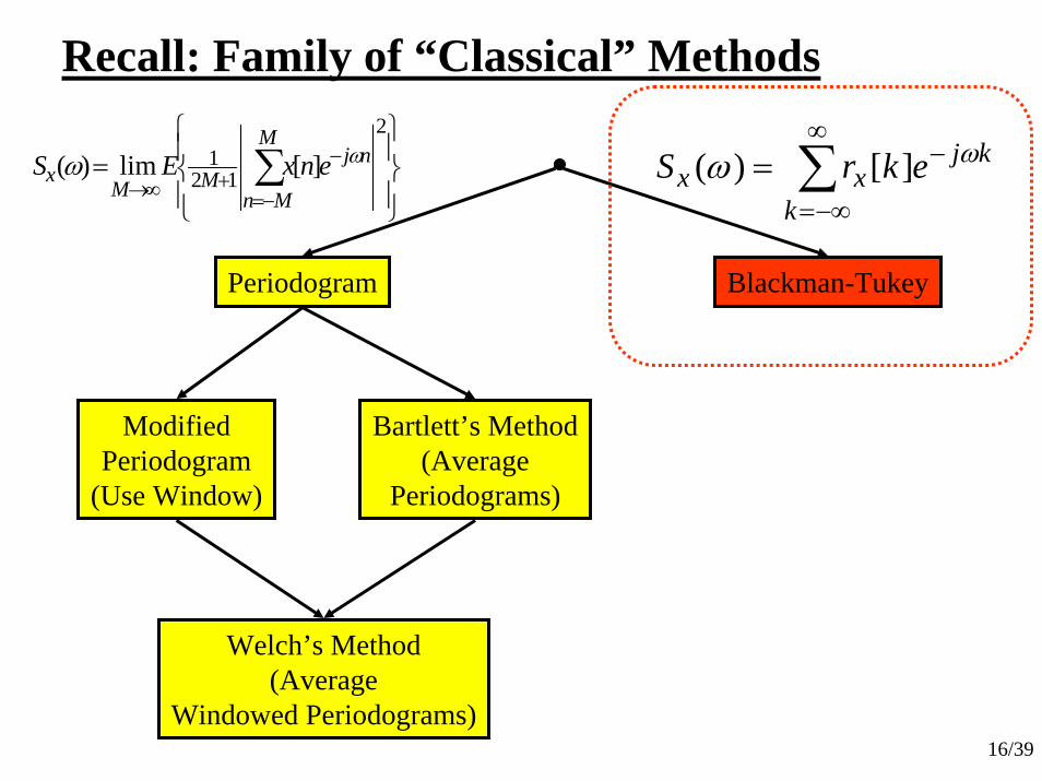
Recall: Family of “Classical” Methods
Periodogram
ModifiedPeriodogram
(Use Window)
Bartlett’s Method(Average
Periodograms)
Welch’s Method(Average
Windowed Periodograms)
Blackman-Tukey
⎪⎭
⎪⎬⎫
⎪⎩
⎪⎨⎧
= ∑−=
−+∞→
2
121 ][lim)(
M
Mn
njMM
x enxES ωω ∑∞
−∞=
−=k
kjxx ekrS ωω ][)(
5/39
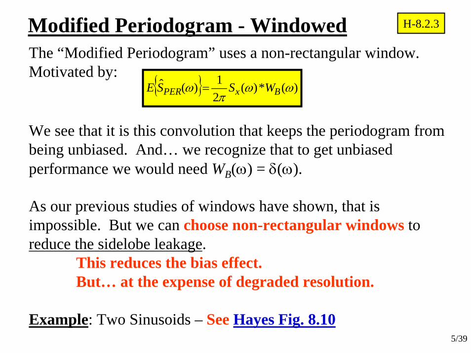
Modified Periodogram - WindowedThe “Modified Periodogram” uses a non-rectangular window. Motivated by:
{ } )(*)(21)(ˆ ωωπ
ω BxPER WSSE =
We see that it is this convolution that keeps the periodogram from being unbiased. And… we recognize that to get unbiased performance we would need WB(ω) = δ(ω).
As our previous studies of windows have shown, that is impossible. But we can choose non-rectangular windows to reduce the sidelobe leakage.
This reduces the bias effect.But… at the expense of degraded resolution.
Example: Two Sinusoids – See Hayes Fig. 8.10
H-8.2.3
6/39
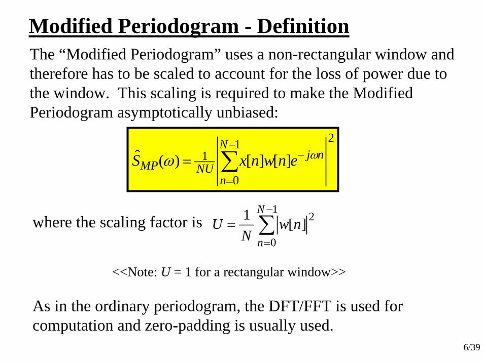
Modified Periodogram - DefinitionThe “Modified Periodogram” uses a non-rectangular window and therefore has to be scaled to account for the loss of power due to the window. This scaling is required to make the Modified Periodogram asymptotically unbiased:
21
0
1 ][][)(ˆ ∑−
=
−=N
n
njNUMP enwnxS ωω
where the scaling factor is ∑−
==
1
0
2][1 N
nnw
NU
<<Note: U = 1 for a rectangular window>>
As in the ordinary periodogram, the DFT/FFT is used for computation and zero-padding is usually used.
7/39
Modified Periodogram - PerformanceThe Modified Periodogram:
• Has reduced bias but is still biased.• Is asymptotically unbiased.• Has variance that roughly equals that of the periodogram.
8/39
Bartlett’s Method: Averaged PeriodogramOne of the main flaws in the periodogram is the lack of averaging.
<< See how ensemble averaging improves it… Hayes Fig. 8.8>>
This lack of averaging is what leads to the non-decreasing variance as well as the rapid fluctuations of the periodogram.
Now… in practice we have only one realization…So what do we do to allow averaging????
We HOPE that the process is ergodic!!!!A process is ergodic if time averaging of any realization is equivalent to ensemble averaging.
H-8.2.4
9/39
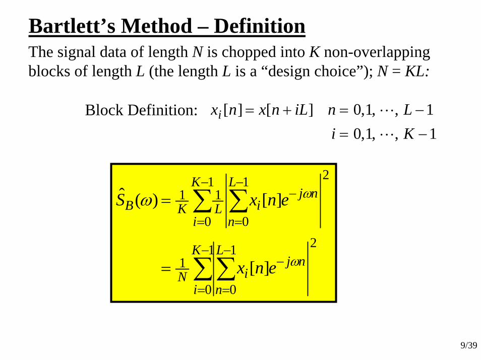
Bartlett’s Method – DefinitionThe signal data of length N is chopped into K non-overlapping blocks of length L (the length L is a “design choice”); N = KL:
1,,1,01,,1,0][][−=−=+=
KiLniLnxnxi
∑∑
∑ ∑
−
=
−
=
−
−
=
−
=
−
=
=
1
0
21
0
1
1
0
21
0
11
][
][)(ˆ
K
i
L
n
njiN
K
i
L
n
njiLKB
enx
enxS
ω
ωω
Block Definition:
10/39
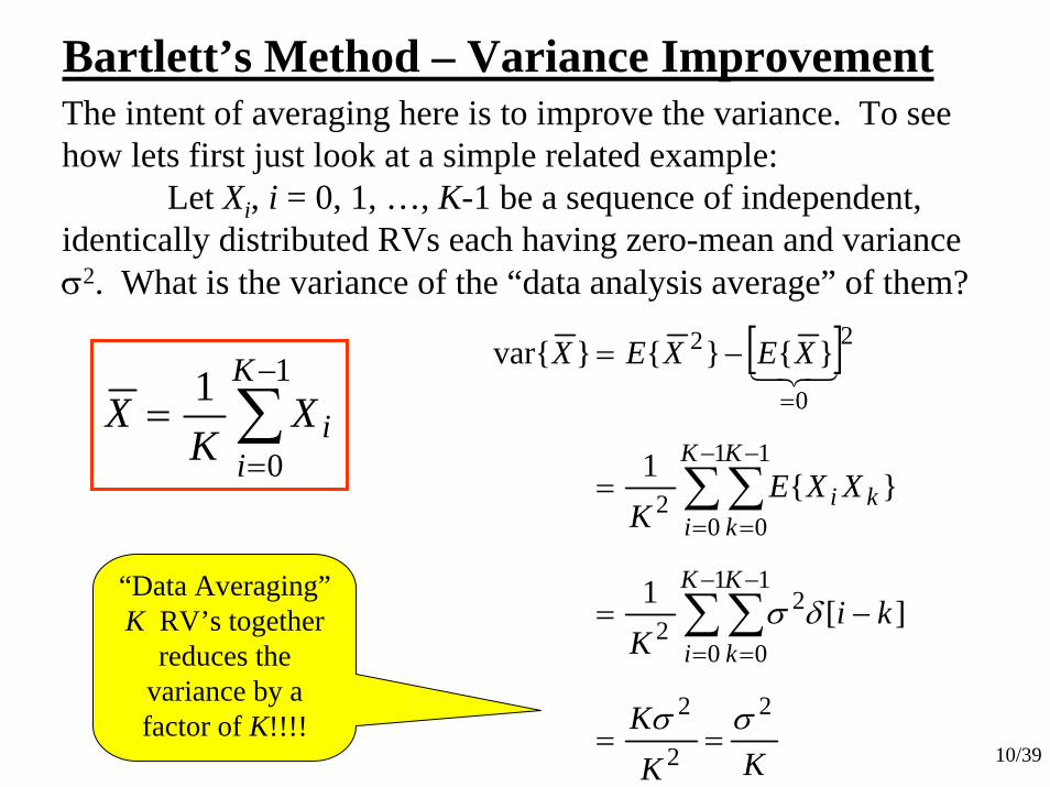
Bartlett’s Method – Variance ImprovementThe intent of averaging here is to improve the variance. To seehow lets first just look at a simple related example:
Let Xi, i = 0, 1, …, K-1 be a sequence of independent, identically distributed RVs each having zero-mean and variance σ2. What is the variance of the “data analysis average” of them?
∑−
==
1
0
1 K
iiX
KX
“Data Averaging”K RV’s together
reduces the variance by a factor of K!!!!
[ ]
KKK
kiK
XXEK
XEXEX
K
i
K
k
K
i
K
kki
2
2
2
1
0
1
0
22
1
0
1
02
2
0
2
][1
}{1
}{}{}var{
σσ
δσ
==
−=
=
−=
∑∑
∑∑
−
=
−
=
−
=
−
=
=
11/39
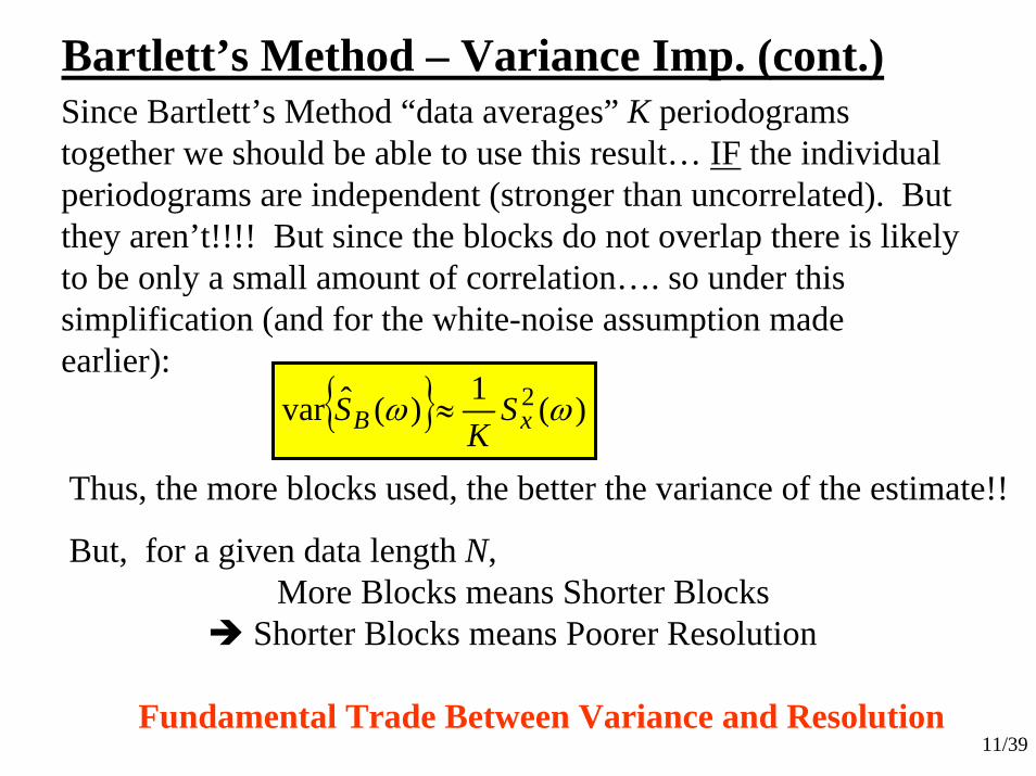
Bartlett’s Method – Variance Imp. (cont.)Since Bartlett’s Method “data averages” K periodograms together we should be able to use this result… IF the individual periodograms are independent (stronger than uncorrelated). But they aren’t!!!! But since the blocks do not overlap there is likely to be only a small amount of correlation…. so under this simplification (and for the white-noise assumption made earlier):
{ } )(1)(ˆvar 2 ωω xB SK
S ≈
Thus, the more blocks used, the better the variance of the estimate!!
But, for a given data length N, More Blocks means Shorter Blocks
Shorter Blocks means Poorer Resolution
Fundamental Trade Between Variance and Resolution
12/39
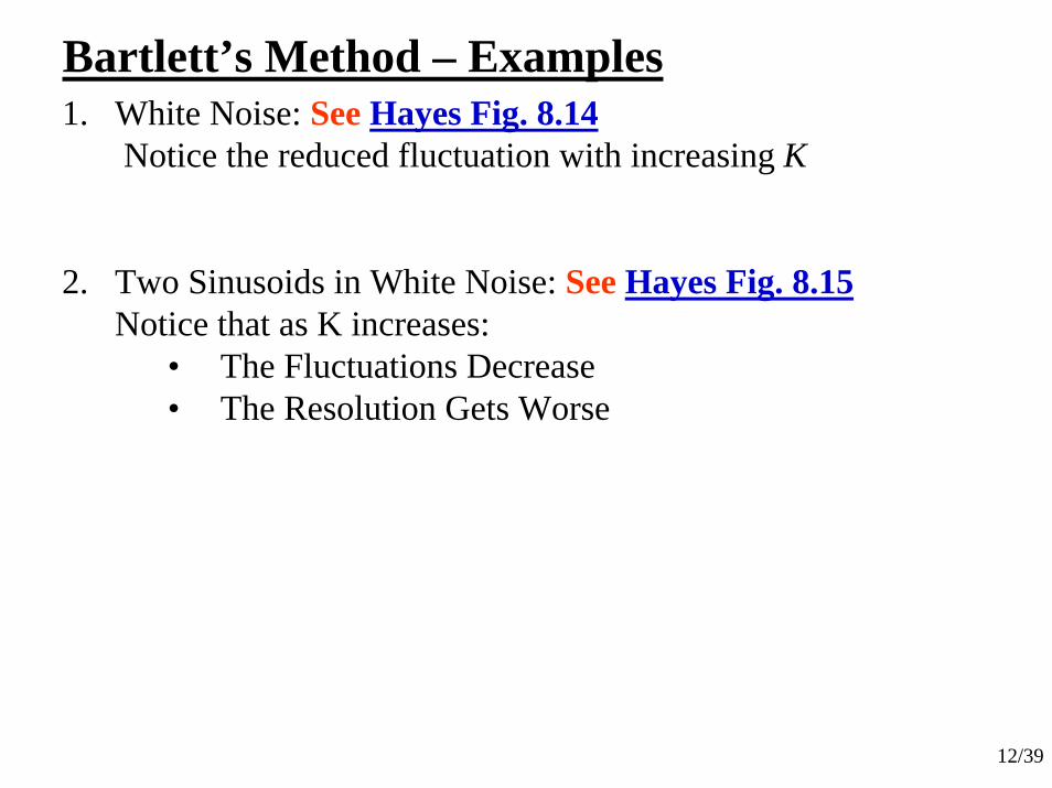
Bartlett’s Method – Examples1. White Noise: See Hayes Fig. 8.14
Notice the reduced fluctuation with increasing K
2. Two Sinusoids in White Noise: See Hayes Fig. 8.15Notice that as K increases:
• The Fluctuations Decrease• The Resolution Gets Worse
13/39
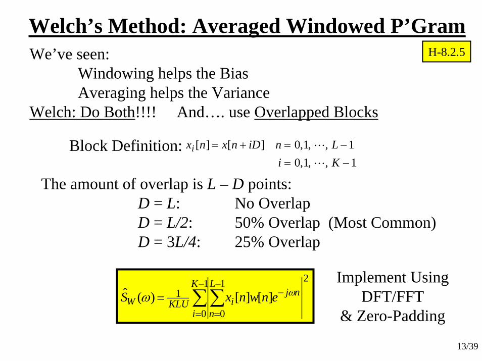
Welch’s Method: Averaged Windowed P’GramWe’ve seen:
Windowing helps the BiasAveraging helps the Variance
Welch: Do Both!!!! And…. use Overlapped Blocks
1,,1,01,,1,0][][−=−=+=
KiLniDnxnxi
∑∑−
=
−
=
−=1
0
21
0
1 ][][)(ˆK
i
L
n
njiKLUW enwnxS ωω
Block Definition:
The amount of overlap is L – D points:D = L: No OverlapD = L/2: 50% Overlap (Most Common)D = 3L/4: 25% Overlap
Implement UsingDFT/FFT
& Zero-Padding
H-8.2.5
14/39
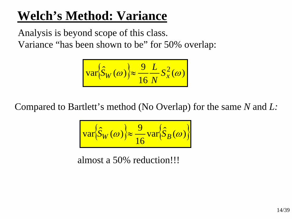
Welch’s Method: VarianceAnalysis is beyond scope of this class.Variance “has been shown to be” for 50% overlap:
{ } )(169)(ˆvar 2 ωω xW S
NLS ≈
Compared to Bartlett’s method (No Overlap) for the same N and L:
{ } { })(ˆvar169)(ˆvar ωω BW SS ≈
almost a 50% reduction!!!
15/39
Modifications Based on ACF View
• Blackman-Tukey Method
16/39
Recall: Family of “Classical” Methods
Periodogram
ModifiedPeriodogram
(Use Window)
Bartlett’s Method(Average
Periodograms)
Welch’s Method(Average
Windowed Periodograms)
Blackman-Tukey
⎪⎭
⎪⎬⎫
⎪⎩
⎪⎨⎧
= ∑−=
−+∞→
2
121 ][lim)(
M
Mn
njMM
x enxES ωω ∑∞
−∞=
−=k
kjxx ekrS ωω ][)(
17/39
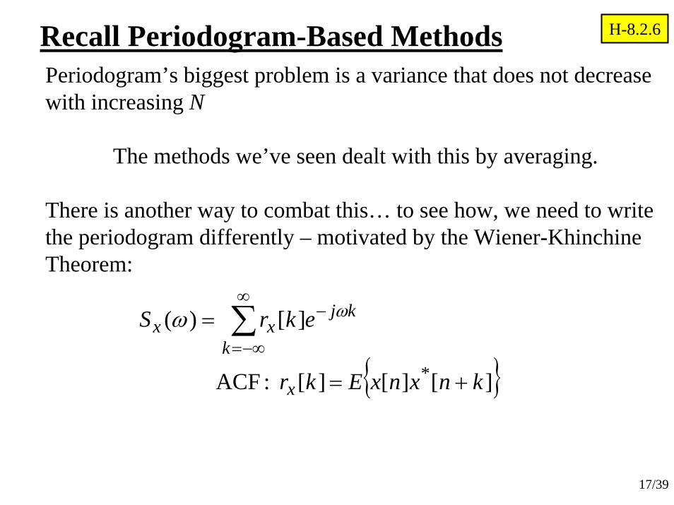
Recall Periodogram-Based MethodsPeriodogram’s biggest problem is a variance that does not decrease with increasing N
The methods we’ve seen dealt with this by averaging.
There is another way to combat this… to see how, we need to write the periodogram differently – motivated by the Wiener-KhinchineTheorem:
{ }][][][ :ACF
][)(
* knxnxEkr
ekrS
x
k
kjxx
+=
= ∑∞
−∞=
− ωω
H-8.2.6
18/39
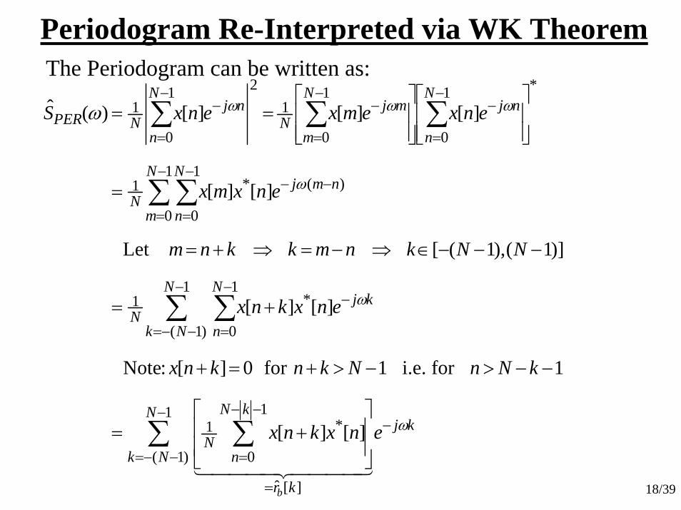
∑ ∑
∑ ∑
∑∑
∑∑∑
−
−−=
−
=
−−
=
−
−−=
−
=
−
−
=
−
=
−−
−
=
−−
=
−−
=
−
⎥⎥
⎦
⎤
⎢⎢
⎣
⎡+=
−−>−>+=+
+=
−−−∈⇒−=⇒+=
=
⎥⎥⎦
⎤
⎢⎢⎣
⎡
⎥⎥⎦
⎤
⎢⎢⎣
⎡==
1
)1(
][ˆ
1
0
*1
1
)1(
1
0
*1
1
0
1
0
)(*1
*1
0
1
0
121
0
1
][][
1for i.e.1for 0][ :Note
][][
)]1(),1([Let
][][
][][][)(ˆ
N
Nk
kj
kr
kN
nN
N
Nk
N
n
kjN
N
m
N
n
nmjN
N
n
njN
m
mjN
N
n
njNPER
enxknx
kNnNknknx
enxknx
NNknmkknm
enxmx
enxemxenxS
b
ω
ω
ω
ωωωω
Periodogram Re-Interpreted via WK TheoremThe Periodogram can be written as:
19/39
∑−
−−=
−=1
)1(][ˆ)(ˆ
N
Nk
kjbPER ekrS ωω
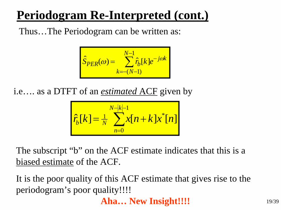
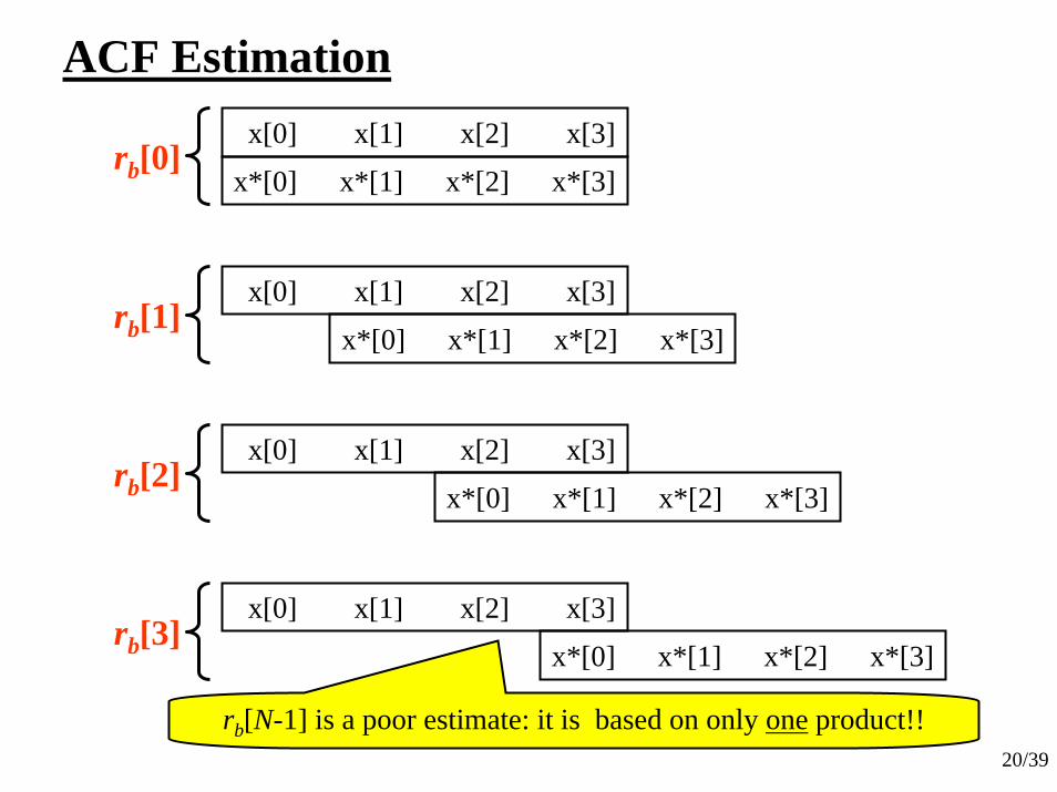
Periodogram Re-Interpreted (cont.)Thus…The Periodogram can be written as:
i.e…. as a DTFT of an estimated ACF given by
∑−−
=
+=1
0
*1 ][][][ˆkN
nNb nxknxkr
The subscript “b” on the ACF estimate indicates that this is a biased estimate of the ACF.
It is the poor quality of this ACF estimate that gives rise to the periodogram’s poor quality!!!!
Aha… New Insight!!!!
20/39
ACF Estimationx[0] x[1] x[2] x[3]
x*[0] x*[1] x*[2] x*[3]rb[0]
x[0] x[1] x[2] x[3]x*[0] x*[1] x*[2] x*[3]
rb[1]
x[0] x[1] x[2] x[3]x*[0] x*[1] x*[2] x*[3]
rb[2]
x[0] x[1] x[2] x[3]x*[0] x*[1] x*[2] x*[3]
rb[3]
rb[N-1] is a poor estimate: it is based on only one product!!
21/39
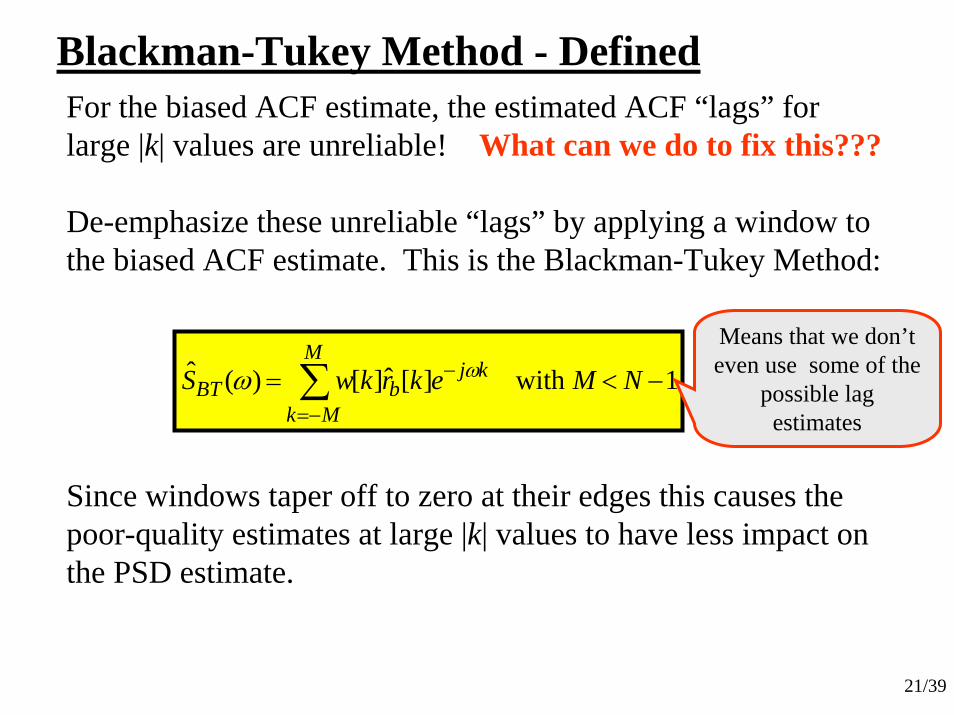
Blackman-Tukey Method - DefinedFor the biased ACF estimate, the estimated ACF “lags” for large |k| values are unreliable! What can we do to fix this???
De-emphasize these unreliable “lags” by applying a window to the biased ACF estimate. This is the Blackman-Tukey Method:
1 with][ˆ][)(ˆ −<= ∑−=
− NMekrkwSM
Mk
kjbBT
ωω
Since windows taper off to zero at their edges this causes the poor-quality estimates at large |k| values to have less impact on the PSD estimate.
Means that we don’t even use some of the
possible lag estimates
22/39
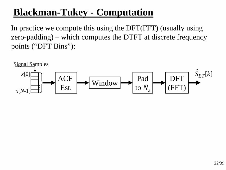
Blackman-Tukey - ComputationIn practice we compute this using the DFT(FFT) (usually using zero-padding) – which computes the DTFT at discrete frequency points (“DFT Bins”):
Padto Nz
Signal Samples
x[0]
x[N-1]
DFT(FFT)
][ˆ kSBTACF Est. Window
23/39
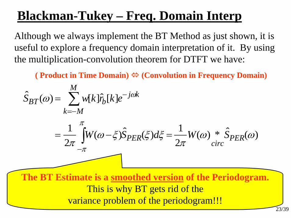
Blackman-Tukey – Freq. Domain InterpAlthough we always implement the BT Method as just shown, it is useful to explore a frequency domain interpretation of it. By using the multiplication-convolution theorem for DTFT we have:
)(ˆ*)(21)(ˆ)(
21
][ˆ][)(ˆ
ωωπ
ξξξωπ
ω
π
π
ω
PERcirc
PER
M
Mk
kjbBT
SWdSW
ekrkwS
=−=
=
∫
∑
−
−=
−
( Product in Time Domain) (Convolution in Frequency Domain)
The BT Estimate is a smoothed version of the Periodogram.This is why BT gets rid of the
variance problem of the periodogram!!!
24/39
Blackman-Tukey vs. Welch/Bartlett MethodBoth the BT method and the Welch/Bartlett method are successful in reducing the variance compared to the pure Periodogram. But HOW they do it is quite different!
• Welch/Bartlett does it by averaging away the variations over many computed periodograms.
• Blackman-Tukey does it by smoothing the variations out of a single periodogram.
25/39
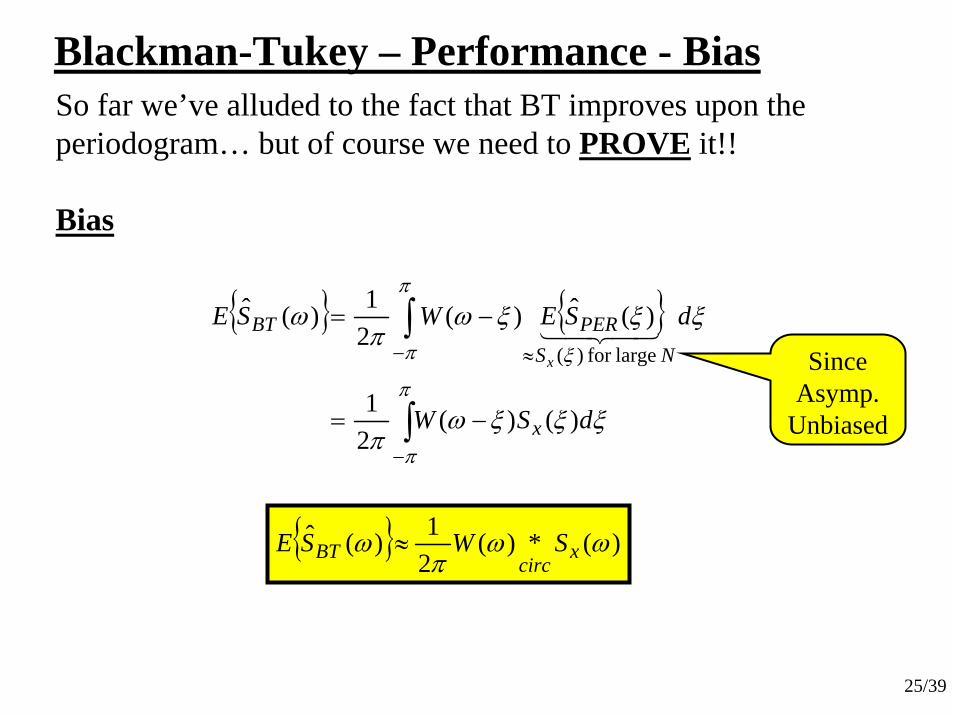
Blackman-Tukey – Performance - BiasSo far we’ve alluded to the fact that BT improves upon the periodogram… but of course we need to PROVE it!!
Bias
{ } { }
∫
∫
−
− ≈
−=
−=
π
π
π
π ξ
ξξξωπ
ξξξωπ
ω
dSW
dSEWSE
x
NSPERBT
x
)()(21
)(ˆ)(21)(ˆ
largefor )(
{ } )(*)(21)(ˆ ωωπ
ω xcirc
BT SWSE ≈
Since Asymp.
Unbiased
26/39
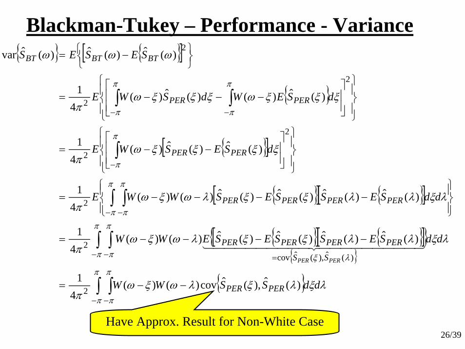
Blackman-Tukey – Performance - Variance{ } { }[ ]
{ }
{ }[ ]
{ }[ ] { }[ ]
{ }[ ] { }[ ]{ }{ }
{ }∫ ∫
∫ ∫
∫ ∫
∫
∫∫
− −
− − =
− −
−
−−
−−=
−−−−=
⎪⎭
⎪⎬⎫
⎪⎩
⎪⎨⎧
−−−−=
⎪⎭
⎪⎬
⎫
⎪⎩
⎪⎨
⎧
⎥⎥⎦
⎤
⎢⎢⎣
⎡−−=
⎪⎭
⎪⎬
⎫
⎪⎩
⎪⎨
⎧
⎥⎥⎦
⎤
⎢⎢⎣
⎡−−−=
⎭⎬⎫
⎩⎨⎧ −=
π
π
π
π
π
π
π
π λξ
π
π
π
π
π
π
π
π
π
π
λξλξλωξωπ
λξλλξξλωξωπ
λξλλξξλωξωπ
ξξξξωπ
ξξξωξξξωπ
ωωω
ddSSWW
ddSESSESEWW
ddSESSESWWE
dSESWE
dSEWdSWE
SESES
PERPER
SS
PERPERPERPER
PERPERPERPER
PERPER
PERPER
BTBTBT
PERPER
)(ˆ),(ˆcov)()(4
1
)(ˆ)(ˆ)(ˆ)(ˆ)()(4
1
)(ˆ)(ˆ)(ˆ)(ˆ)()(4
1
)(ˆ)(ˆ)(4
1
)(ˆ)()(ˆ)(4
1
)(ˆ)(ˆ)(ˆvar
2
)(ˆ),(ˆcov2
2
2
2
2
2
2
Have Approx. Result for Non-White Case
27/39
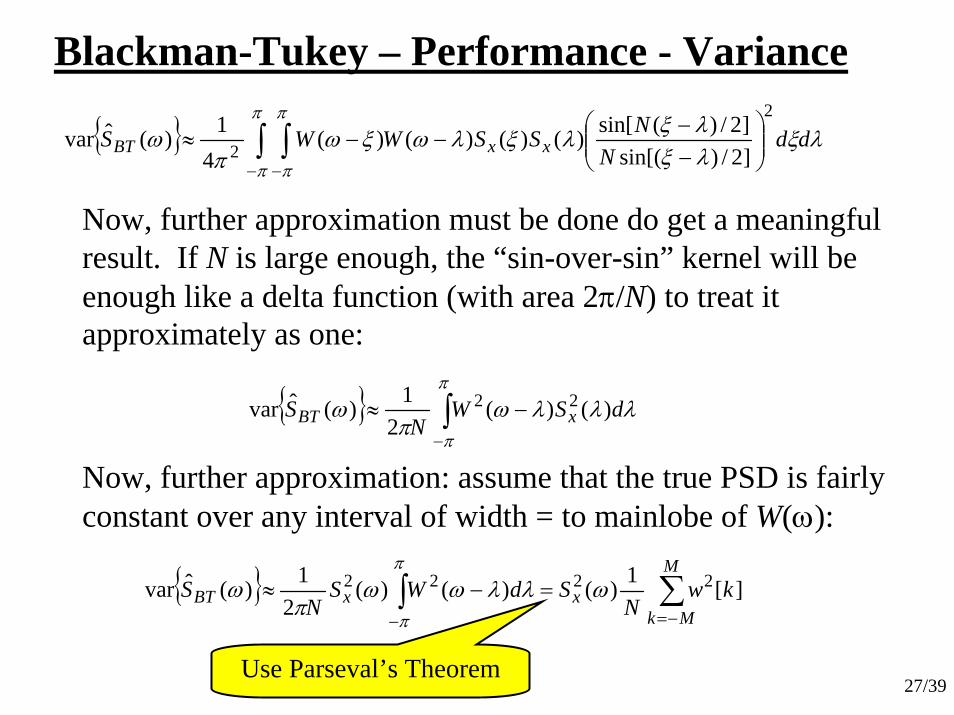
Blackman-Tukey – Performance - Variance
{ } ∫ ∫− −
⎟⎟⎠
⎞⎜⎜⎝
⎛−−
−−≈π
π
π
π
λξλξλξλξλωξω
πω dd
NNSSWWS xxBT
2
2 ]2/)sin[(]2/)(sin[)()()()(
41)(ˆvar
Now, further approximation must be done do get a meaningful result. If N is large enough, the “sin-over-sin” kernel will be enough like a delta function (with area 2π/N) to treat it approximately as one:
{ } ∫−
−≈π
π
λλλωπ
ω dSWN
S xBT )()(2
1)(ˆvar 22
Now, further approximation: assume that the true PSD is fairly constant over any interval of width = to mainlobe of W(ω):
{ } ∑∫−=−
=−≈M
MkxxBT kw
NSdWS
NS ][1)()()(
21)(ˆvar 2222 ωλλωωπ
ωπ
π
Use Parseval’s Theorem
28/39
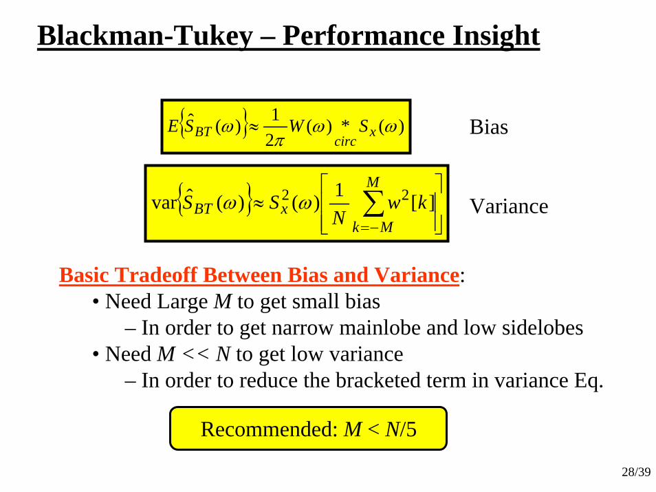
Blackman-Tukey – Performance Insight
{ }⎥⎥⎦
⎤
⎢⎢⎣
⎡≈ ∑
−=
M
MkxBT kw
NSS ][1)()(ˆvar 22 ωω
{ } )(*)(21)(ˆ ωωπ
ω xcirc
BT SWSE ≈ Bias
Variance
Basic Tradeoff Between Bias and Variance:• Need Large M to get small bias
– In order to get narrow mainlobe and low sidelobes• Need M << N to get low variance
– In order to reduce the bracketed term in variance Eq.
Recommended: M < N/5
29/39
Performance Comparison for Classical Methods
H-8.2.7
30/39
Performance MeasuresWe’ve seen that we care about three main things:
1. Bias2. Variance3. Resolution
… and there is usually a tradeoff between them – especially between variance & resolution.
It is desirable to come up with a single-measure way tocompare the methods:
Figure-of-Merit = (Variability)×(Resolution)
Combined into “Variability” – see below
31/39
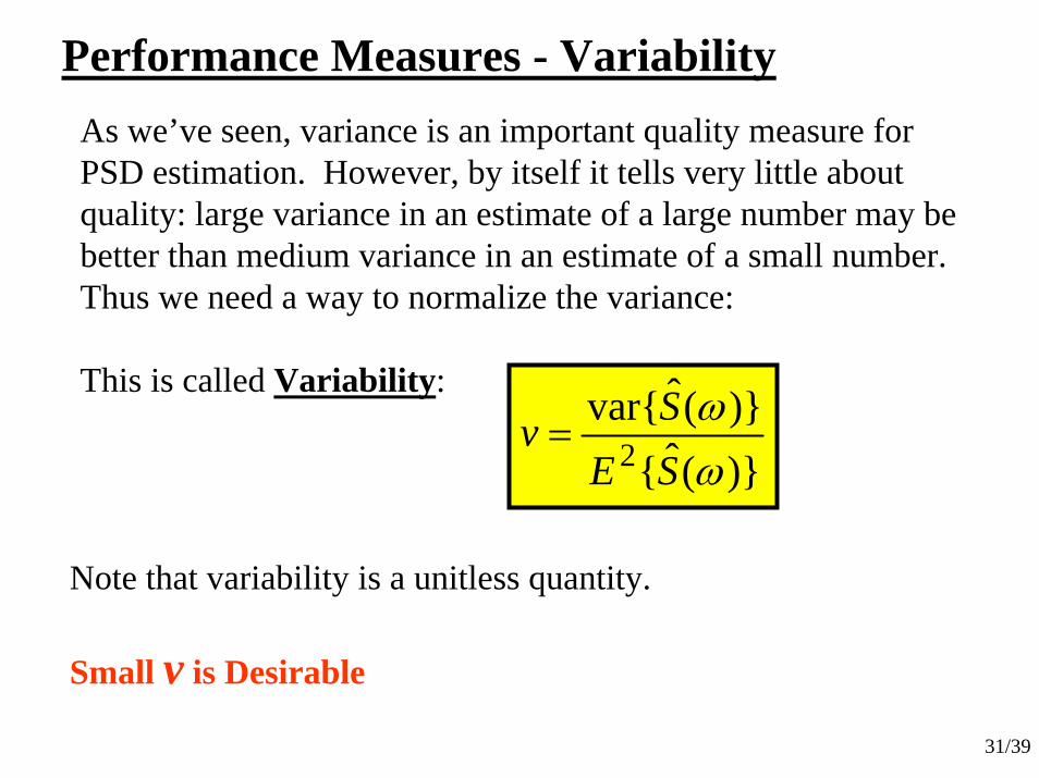
Performance Measures - VariabilityAs we’ve seen, variance is an important quality measure for PSD estimation. However, by itself it tells very little about quality: large variance in an estimate of a large number may be better than medium variance in an estimate of a small number.Thus we need a way to normalize the variance:
This is called Variability:
)}(ˆ{)}(ˆvar{
2 ωω
SESv =
Note that variability is a unitless quantity.
Small v is Desirable
32/39
Performance Measures - ResolutionAs we saw in our studies of Ch. 6 in Porat, one of the important measures of goodness for spectral analysis is resolution – the ability to see two closely-spaced sinusoids.
Recall: The width of the mainlobe of the window’s kernel impacts this ability. There are many ways to measure resolution – Hayes defines resolution as:
Mainlobeof Width dB 6=Δω
Small Δω is Desirable
Recall – Two things impact ML Width:1. Window Length: Δω↓ as Length ↑2. Window Shape (e.g. Hanning, Hamming, Etc.)
Recall – There is a tradeoff between Δω and SL level
33/39
Overall Figure of MeritIt is helpful to have a single measure by which to compare methods. This is done using the following Figure of Merit:
ωΔ×= vM
Since v and Δω are both required to be as small as possible, we also want the figure of merit M to be as small as possible.
34/39
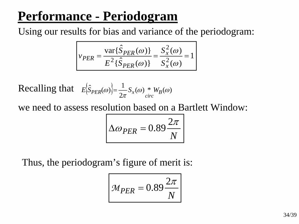
Performance - Periodogram
1)()(
)}(ˆ{)}(ˆvar{
2
2
2 ===ωω
ωω
x
x
PER
PERPER
SS
SESv
Using our results for bias and variance of the periodogram:
Recalling that { } )(*)(21)(ˆ ωωπ
ω Bcirc
xPER WSSE =
we need to assess resolution based on a Bartlett Window:
NPERπω 289.0=Δ
Thus, the periodogram’s figure of merit is:
NPERπ289.0=M
35/39
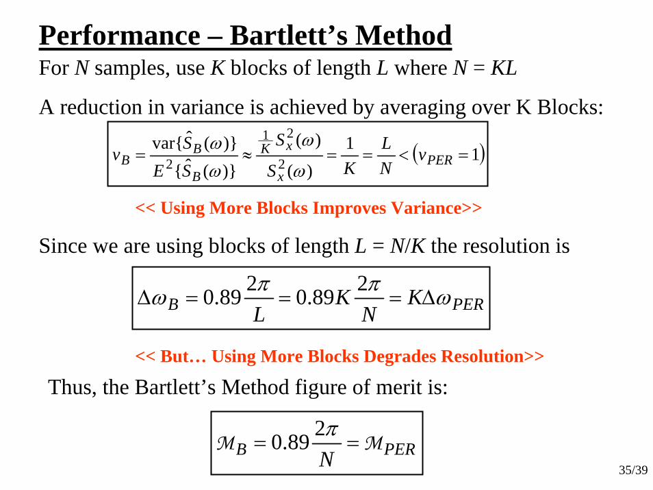
Performance – Bartlett’s Method
( )11)(
)(
)}(ˆ{)}(ˆvar{
2
21
2 =<==≈= PERx
xK
B
BB v
NL
KS
S
SESv
ω
ω
ωω
For N samples, use K blocks of length L where N = KL
A reduction in variance is achieved by averaging over K Blocks:
Since we are using blocks of length L = N/K the resolution is
PERB KN
KL
ωππω Δ===Δ289.0289.0
Thus, the Bartlett’s Method figure of merit is:
PERB NMM ==
π289.0
<< Using More Blocks Improves Variance>>
<< But… Using More Blocks Degrades Resolution>>
36/39
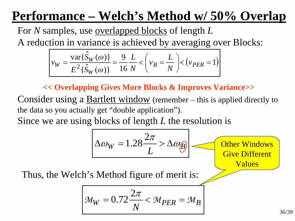
Performance – Welch’s Method w/ 50% Overlap
( )1169
)}(ˆ{)}(ˆvar{
2 =<⎟⎠⎞
⎜⎝⎛ =<== PERB
W
WW v
NLv
NL
SESv
ωω
For N samples, use overlapped blocks of length LA reduction in variance is achieved by averaging over Blocks:
Consider using a Bartlett window (remember – this is applied directly to the data so you actually get “double application”).Since we are using blocks of length L the resolution is
BW Lωπω Δ>=Δ
228.1
Thus, the Welch’s Method figure of merit is:
BPERW NMMM =<=
π272.0
<< Overlapping Gives More Blocks & Improves Variance>>
Other Windows Give Different
Values
Other Windows Give Different
Values
37/39
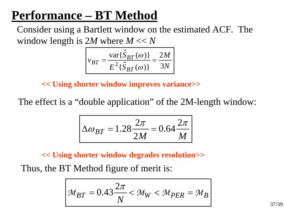
Performance – BT Method
NM
SESv
BT
BTBT 3
2)}(ˆ{)}(ˆvar{
2 ==ωω
Consider using a Bartlett window on the estimated ACF. The window length is 2M where M << N
MMBTππω 264.0
2228.1 ==Δ
Thus, the BT Method figure of merit is:
BPERWBT NMMMM =<<=
π243.0
<< Using shorter window improves variance>>
The effect is a “double application” of the 2M-length window:
<< Using shorter window degrades resolution>>
38/39
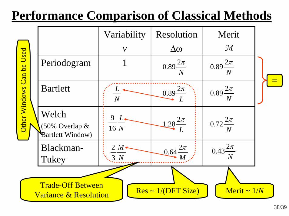
Performance Comparison of Classical MethodsVariability
vResolution
ΔωMeritM
Periodogram 1
Bartlett
Welch(50% Overlap & Bartlett Window)
Blackman-Tukey
NL
NL
169
NM
32
Nπ289.0
Lπ289.0
Lπ228.1
Mπ264.0
Nπ289.0
Nπ289.0
Nπ272.0
Nπ243.0
Merit ~ 1/NTrade-Off Between
Variance & Resolution
=
Res ~ 1/(DFT Size)
Oth
er W
indo
ws C
an b
e U
sed
39/39
Complexity Comparison of Classical Methods
Welch and BT methods are the most commonly used ones. But counting the number of complex multiplies needed for each one, it is easy to see that:
Welch requires a bit more computation then BT
BUT… bear in mind: For BT, none of the ACF lags can be estimated until ALL of the data is obtained – therefore no computing can be done until all the data is obtained
For Welch, DFT’s can be started as soon as each block arrives.
Welch MIGHT have a real-time advantage!!!
Recommended