Portfolio Analysis, Market Equilibrium and Corporation Finance
Robert S. Hamada
The Journal of Finance, Vol. 24, No. 1. (Mar., 1969), pp. 13-31.
Stable URL:
http://links.jstor.org/sici?sici=0022-1082%28196903%2924%3A1%3C13%3APAMEAC%3E2.0.CO%3B2-X
The Journal of Finance is currently published by American Finance Association.
Your use of the JSTOR archive indicates your acceptance of JSTOR's Terms and Conditions of Use, available athttp://www.jstor.org/about/terms.html. JSTOR's Terms and Conditions of Use provides, in part, that unless you have obtainedprior permission, you may not download an entire issue of a journal or multiple copies of articles, and you may use content inthe JSTOR archive only for your personal, non-commercial use.
Please contact the publisher regarding any further use of this work. Publisher contact information may be obtained athttp://www.jstor.org/journals/afina.html.
Each copy of any part of a JSTOR transmission must contain the same copyright notice that appears on the screen or printedpage of such transmission.
The JSTOR Archive is a trusted digital repository providing for long-term preservation and access to leading academicjournals and scholarly literature from around the world. The Archive is supported by libraries, scholarly societies, publishers,and foundations. It is an initiative of JSTOR, a not-for-profit organization with a mission to help the scholarly community takeadvantage of advances in technology. For more information regarding JSTOR, please contact [email protected].
http://www.jstor.orgSun Oct 21 08:58:28 2007
PORTFOLIO ANALYSIS, MARKET EQUILIBRIUM AND CORPORATION FINANCE
AT LEAST THREE conceptual frameworks have been developed to study the effects of uncertainty on financial and economic decision-making in recent times. Of these, the homogenous risk-class concept constructed to eliminate the need for a general equilibrium model by Modigliani and Miller [20, 2 1, 221, henceforth abbreviated to MM, is most familiar to those interested in corpora- tion finance. On the other hand, the most common basis for making personal or institutional investment decisions is the portfolio model first developed by Markowitz [16, 171. Little has been developed rigorously to cross the finance fields using either of these two uncertainty frameworks.'
More recently, a third uncertainty model has been revived by Hirshleifer [8, 9, 101 and labeled the time-state preference approach.' This last model is undoubtedly the most general approach to uncertainty and was used by Hirshleifer [ lo] to prove the famous MM no-tax Proposition I. Unfortunately, thus far, this generality has its cost. Using a time-state preference formulation, it is difficult to test its propositions empirically (since markets do not exist for each state) or to derive practical decision rules for capital budgeting within the firm.
The purpose of this paper is to derive the three MM Propositions using the standard deviation-mean portfolio model in a market equilibrium context. This approach to some of the major issues of corporation finance enables us to derive these propositions in a somewhat more direct way than with the use of the risk-class assumption and the arbitrage proof of the MM paper. Instead, a model is substituted relating the maximization of stockholder expected utility to the seIection of portfoIios of assets to, finaIIy, the financing and invest- ment decisions within the corporation. A link will be provided between two branches of the field of finance that have so far been evolving more or less separately.
In Section 11, the assumptions are enumerated and the equilibrium capital asset pricing model is presented. MM's Propositions I and 11, the effects of
* Graduate School of Business, University of Chicago. The generous support of the Ford Foundation and the research committee of the Graduate School of Business is gratefully acknowledged. I am indebted to Eugene Fama, Merton Miller, and Myron Scholes for their helpful comments in the preparation of this paper.
1. The notable exception is the article by Lintner [I31 which considered corporate capital budgeting questions in the context of a market equilibrium portfolio model. Lintner's treatment of this problem will be discussed in Section V.
2. Hirshleifer restated the Arrow-Debreu [I, 41 objects of choice in the classical Irving Fisher 171 framework, where the objects ~f choice are consumption or income bundles at explicit times and states-of-the-world,
14 The Journal of Finance
the financing decision on equity prices, are proved in Section I11 for the no corporate income tax case. Section IV is devoted to the corporate tax effect on this financing decision. A derivation and discussion of the cost of capital for investment decisions within the firm (MM's Proposition 111) in the no-tax case are the topics of Section V. And in Section VI, the cost of capital considering corporate taxes is derived.
A. Assumptions
The assumptions are divided into two sets. The following are required for the portfolio-capital asset pricing model:
1) There are perfect capital markets. This implies that information is available to all at no cost, there are no taxes and no transaction costs, and all assets are infinitely divisible. Also, all investors can borrow or lend at the same rate of interest and have the same portfolio opportunities.
2 ) Investors are risk-averters and maximize their expected utility of wealth at the end of their planning horizon or the one-period rate of return over this h ~ r i z o n . ~In addition, it is assumed that portfolios can be assessed solely by their expected rate of return and standard deviation of this rate of return. Of two portfolios with the same standard deviation, the criterion of choice would lead to the selection of that portfolio with the greater mean; and of two portfolios with the same expected rate of return, the investor would select the one with the smaller risk as measured by the standard deviation. This implies that either the investor's utility function is quadratic or that port- folio rates of return are multivariate normal.'
3 ) The planning horizon is the same for all investors and their portfolio decisions made at the same time.
4) All investors have identical estimates of expected rates of return and the standard deviations of these rates.6
In addition to these four assumptions, we shall require the following for the subsequent sections :
5) Expected bankruptcy or default risk associated with debt-financing, as well as the risk of interest rate and purchasing power fluctuation, are assumed to be negligible relative to variability risk on equity. Thus, the
3. The first two sections of Fama's paper 161 is recommended as the clearest exposition of this model for the homogeneous expectations case. The extension to the case of differing judgments by investors can be found in Bierwag and Grove [2] and Lintner [14, pp. 600-6011. We shall not use the heterogeneous expectations framework here since it will not add to the primary purpose of this paper and may only serve to take the focus away from our major concern.
4. The rate of return is defined as the change in wealth divided by the investor's initial wealth, where the change in wealth includes dividends and capital gains. Note that this is a one-period model, in common with Lintner's 113, 141 and in many respects with MM's 120, 21, 221.
5. See Tobin [27, pages 82-85] for a justification; the need for the restrictive normal probability distribution assumption is not strictly required, as Fama 151 has generalized much of the results of the Sharpe-Lintner model for other members of the stable class of distributions where the standard deviation does not exist. I t can be further noted, as Lintner [13, pages 18-191 does, that Roy [241 has shown that investors who minimize the probability of disaster (who use the "safety-first" principle) will have roughly the same investment criterion for risky assets. 6.See footnote 3.
15 Portfolio Analysis and Market Equilibriuln
corporation is assumed to be able to borrow or lend a t the same risk-free rate as the individual investor.
6) Dividend policy is assumed to have no effect on the market value of a firm's equity or cost of capital. Having made our initial assumption of perfect capital markets, i t was shown by MM in [19] that this need not be an addi- tional assumption as long as there is rational investor behavior and the financing and investment policies of the corporation can be considered inde- pendent. If assumption (5) is valid, this second requirement should be met.
7) Though future investment opportunities available to the firm at rates of return greater than the cost of capital undoubtedly are reflected in the current market price, we shall ignore them here. They can be considered a capitalized quantity independent of the issues raised by MM's three proposi- tions as long as the firm has a long-run financing policy (if the financing mix affects the cost of capital) and if the marginal rate of return of a new invest- ment (to be compared to the subsequently derived cost of capital) includes all, direct and indirect, contributions to cash flow provided by this in~estment .~
B. Asset Prices and Market Equilibrium
Represent the rate of return of a portfolio or risky asset by the random variable R. From assumption (2), the expected rate of return, E ( R ) , and the standard deviation, o(R) , of portfolios are the objects of choice; this leads to the formation, by each individual investor, of an efficient set of risky portfolios according to the principles provided by Markowitz [16, 171. Intro- ducing a riskless asset with a rate of return RF leads to a new efficient set combining a single risky portfolio, M (which was on the previous efficient set), with various proportions of the risk-free asset (this includes borrowing as well as lending).
Because maximum expected utility for a risk-averter requires a tangency of his expected utility curve with this efficient set, and because all investors have the same expectations, risky portfolio M would be combined by all investors in some proportion with the riskless asset. And market equilibrium requires all outstanding risky assets to be held in the proportion of their market value to the total market value of all assets. This is the composition of portfolio M, henceforth called the market portfolio.
From this construct, the following Sharpe-Lintner-Mossin [ 2 5 , 13, 14, 231 equilibrium relationship can be derived for any individual risky asset i in the market:8
7 . This latter requirement is the issue raised by Miller in 1181 on Lintner's growth papers [ll , 121. Lintner assumed that the indirect effects, such as shifting the firm's inveslment productivity schedule to a more profitable level in all future time periods, are the same for all projects and therefore do not have to he included in the marginal rate of return of the project under con-sideration. Instead, we are requiring that all effects and opportunities introduced by the acceptance of this project be taken into account explicitly in the marginal rate of return. For one practical method of doing this, see Magee [151.
8. See [61 for the derivation of equation (1).
16 The Jourhal of Finance
E (RM)-RFNote that is the same for all assets and can be viewed as a
o2(RM) measure of market risk aversion, or the price of a dollar of risk. Substituting a constant 1 for this expression in (1),we have:
Equation ( l a ) supplies us with a formal market relationship between any asset's required rate of return and its individual risk, as measured by cov (R1, Rnt) .
A. Effect of Leverage on Stockholders' Equity
This section will deal with MM's Proposition I-the effects on equity value and perceived risk as a firm alters its capital structure. The quality of equity will no longer be the same and is directly dependent on the corporation's debt- equity ratio. For this purpose, we have constructed the following: assume equilibrium exists and there is a corporation, A, with no debt in its capital structure. Defining SA as the present equilibrium market value of the equity of this debt-free firm, E(SAT) as the expected market value for this same firm one period later, E(div) as the expected dividends paid over this period, and E(XA) as expected earnings net of depreciation but prior to the deduction of interest and tax payments, assumptions ( 6 ) and (7) allow us to write the following relationship for the dollar return:
Employing the definition of the expected rate of return, we have:
giving us a relation for the rate of return required by corporation A's share- holders.
Now assume that corporation A decides to alter its capital structure with- out changing any of its other policies. This implies its assets, both present and future, remain the same as before. All it decides to do is to simultaneously issue some debt (at the riskless rate, RF) and purchase as much of its equity as it can with the proceeds. Let us denote the equity of this same real firm, after the issuance of debt, as B.9 The rate of return required by the remain- ing stockholders is given by adjusting (2), and thus ( 3 ) :
9. This construction can be readily extended to the cases where a firm already has debt and is considering either increasing or decreasing the proportion of debt in its capital structure. Also, if we rigidly honor the one-period planning horizon restriction, then the situation should be more precisely worded: equilibrium a t t =0 with equity A included and market price for risk X. Firm A adds debt a t t =0+ E and general equilibrium restored immediately with market risk aversion remaining the same, This comparative statics framework will be used throughout this paper.
17 Portfolio Analysis and Market Equilibrium
Two points concerning (4) should be emphasized. First, the earnings from assets is E(XA), since this is the same "real" firm as A. And secondly, the interest payments, RFDB, as noted in assumption ( S ) , is not a random variable.
Next, from ( la ) , the equilibrium required rate of return-risk relationship is substituted into (3) and (4) to yield:1°
Intuitively, equity B should be riskier than A since its dollar return is a residual after fixed interest commitments are paid. Thus, COV(RB, RM) should be greater than c o v ( R ~ , RM). In addition, the expected return to the two equities are different so that it is not immediately clear what the relationship between SA and SB should be in equilibrium. T o pursue this point, rearrange (3a) and (4a) to isolate E(XA)and equate the two relations:
( 5 ) The next step is to note the definition of the covariance:
Similarly: l1
10. 1 is not strictly equal in (3a) and (4a) since one equity, B, has been substituted for an- other, A. Because h includes the effects of all capital assets, the substitution of B for A should have a negligible effect on the value of the market price of risk.
11. If the "feel" for the covariance of asset earnings with Rx is difficult, we can use the defini- tion:
where ST is the market value of all capital assets and T the total number of risky assets, k, out-standing. Then:
1 T cov (XA,RM) =- X cov (XA, Xk) . (6a)
ST k'l
Substituting (6a) into (6) and ( 7 ) , respectively, yields:
1 T cov (RA, R,) =- cov (XA, Xk)
SAST k-1
1 T
18 The Journal of Finance
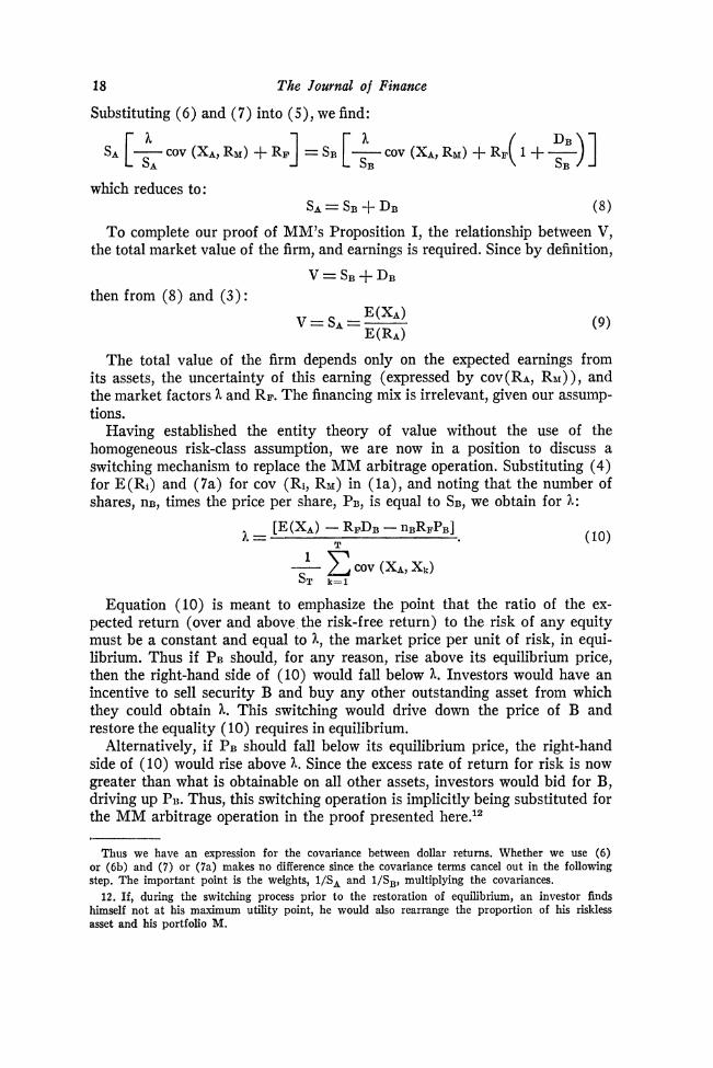
Substituting (6) and ( 7 ) into (S ) , we find:
which reduces to: SA=SB+ DB
To complete our proof of MM's Proposition I, the relationship between V, the total market value of the firm, and earnings is required. Since by definition,
V = S B + D B then from (8) and ( 3 ) :
The total value of the firm depends only on the expected earnings from its assets, the uncertainty of this earning (expressed by c o v ( R ~ , RM)) , and the market factors il and RF. The financing mix is irrelevant, given our assump- tions.
Having established the entity theory of value without the use of the homogeneous risk-class assumption, we are now in a position to discuss a switching mechanism to replace the MM arbitrage operation. Substituting (4) for E(Ri) and (7a) for cov (Ri, Ru) in ( l a ) , and noting that the number of shares, n ~ , times the price per share, PB,is equal to SB, we obtain for A:
Ccov (X*, X,)ST B=l
Equation (10) is meant to emphasize the point that the ratio of the ex- pected return (over and above the risk-free return) to the risk of any equity must be a constant and equal to A, the market price per unit of risk, in equi- librium. Thus if PBshould, for any reason, rise above its equilibrium price, then the right-hand side of (10) would fall below ?L. Investors would have an incentive to sell security B and buy any other outstanding asset from which they could obtain l i . This switching would drive down the price of B and restore the equality (10) requires in equilibrium.
Alternatively, if PBshould fall below its equilibrium price, the right-hand side of (10) would rise above il. Since the excess rate of return for risk is now greater than what is obtainable on all other assets, investors would bid for B, driving up PB.Thus, this switching operation is implicitly being substituted for the MM arbitrage operation in the proof presented here.12
Thus we have an expression for the covariance between dollar returns. Whether we use (6) or (6b) and (7) or (7a) makes no difference since the covariance terms cancel out in the following step. The important point is the weights, l/SA and l/SB, multiplying the covariances.
12. If, during the switching process prior to the restoration of equilibrium, an investor finds himself not at his maximum utility point, he would also rearrange the proportion of his riskless asset and his portfolio M.
19 Portfolio Analysis and Market Equilibrium
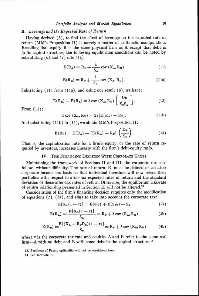
B. Leverage and the Expected Rate of Return
Having derived (8), to find the effect of leverage on the expected rate of return (MM's Proposition 11) is merely a matter of arithmetic manipulation. Recalling that equity B is the same physical firm as A except that debt is in its capital structure, the following equilibrium conditions can be noted by substituting (6) and ( 7 ) into ( l a ) :
Subtracting (1 1) from (1 l a ) , and using our result (8)) we have:
E(RB)-E(Ra)= I cov (XA,RM) -[ 1.s::A (I2) From (11):
A cov (XA,RM)= S b [E(Ra)-RF]. (1 lb)
And substituting ( l l b ) in (12), we obtain MM's Proposition 11:
That is, the capitalization rate for a firm's equity, or the rate of return re-quired by investors, increases linearly with the firm's debt-equity ratio.
IV. THEFINANCING WITH CORPORATE DECISION TAXES Maintaining the framework of Sections I1 and 111,the corporate tax case
follows without difficulty. The rate of return, R, must be defined on an after corporate income tax basis so that individual investors will now select their portfolios with respect to after-tax expected rates of return and the standard deviation of these after-tax rates of return. Otherwise, the equilibrium risk-rate of return relationship presented in Section I1 will not be altered.13
Consideration of the firm's financing decision requires only the modification of equations (2)) (3a), and (4a) to take into account the corporate tax:
where z is the corporate tax rate and equities A and B refer to the same real firm-A with no debt and B with some debt in the capital structure.'*
13. Problems of Pareto optimality will not be considered here. 14. See footnote 10.
20 The Journal of Finance
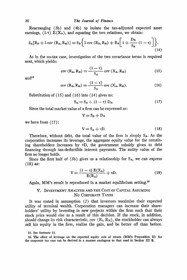
Rearranging (3b) and (4b) to isolate the tax-adjusted expected asset earnings, (1-t) E(XA), and equating the two relations, we obtain:
As in the no-tax case, investigation of the two covariance terms is required next, which yields:
Substitution of (1 5) and (16) into (14) gives us :
Since the total market value of a firm can be expressed as:
we have from (1 7 ) :
Therefore, without debt, the total value of the firm is simply SA. As the corporation increases its leverage, the aggregate equity value for the remain- ing shareholders increases by tD, the government subsidy given to debt financing through tax-deductible interest payments. The entity value of the firm no longer holds.
Since the first half of (3b) gives us a relationship for SA, we can express (18) as:
Again, MM's result is reproduced in a market equilibrium setting.16
I t was stated in assumption ( 2 ) that investors maximize their expected utility of terminal wealth. Corporation managers can increase their share- holders' utility by investing in new projects within the firm such that their stock price would rise as a result of this decision. If the stock, in addition, should change its risk characteristic, cov (Ri, RM), the stockholder can always sell his equity in the firm, realize the gain, and be better off than before.
15. See footnote 11. 16. The effect of leverage on the expected equity rate of return (MM'sProposition 11) for
the corporate tax case can be derived in a manner analogous to that used in Section I11 B.
Portfolio Analysis and Market Equilibriuwt 21
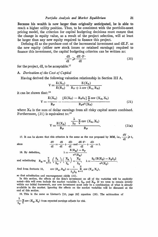
Because his wealth is now larger than originally anticipated, he is able to reach a higher utility position. Thus, to be consistent with the portfolio-asset pricing model, the criterion for capital budgeting decisions must ensure that the change in equity value, as a result of the project selection, will a t least be larger than any new equity required to finance this project.
Defining d I as the purchase cost of the incremental investment and dE.F. as the new equity (either new stock issues or retained earnings) required to finance this investment, the capital budgeting criterion can be written as:
for the project, dI, to be acceptable.17
A. Derivation of the Cost of Capital Having derived the following valuation relationship in Section 111A,
i t can be shown that:18
where XTis the sum of dollar earnings from all risky capital assets combined. Furthermore, (2 1) is equivalent to: l9
dV 17. I t can be shown that this criterion is the same as the one proposed by MM, i.e., -2 1,
dI
since
18. By definition,
T XT ST [E(XT) -RT"STIand substituting R & ~= kEl(s)($) =-, ).= T B ST a2(X,)
1 T And from footnote 11, cov (RA, RM) = 2 CoV ( x ~ , - x,) ,
S S 9-1A T
so that substitution and rearrangement yields (21). In this section, the effects of the firm's investment on all of the variables will be explicitly
noted-this will even include the market variables h, ST, and XT. If we were to remain strictly within our initial framework, any new investment must only be a combination of what is already available in the market. Ignoring the effects on the market variables will be discussed a t the end of this section.
19. This is the same as Lintner's 113, page 261 equation (29). The subtraction of
h -2 cov (X,, Xk) from expected earnings adjusts for risk ST
22 The Journal of Finance
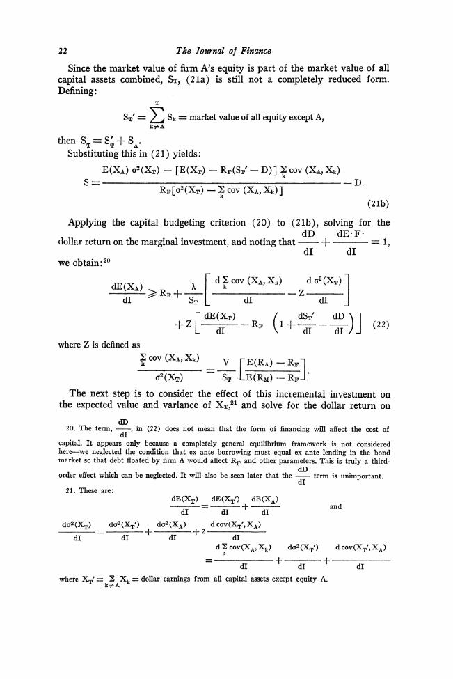
Since the market value of firm A's equity is part of the market value of all capital assets combined, ST, (21a) is still not a completely reduced form. Defining :
T
S d = S k = market value of all equity except A, kZ.4
then ST = S,:, + SA. Substituting this in (2 1) yields:
Applying the capital budgeting criterion (20) to (21b), solving for the
dollar return on the marginal investment, and noting that -dD + dE.F.
= 1,dI dI
we obtain: 20 -
where Z is defined as
The next step is to consider the effect of this incremental investment on the expected value and variance of X~,2land solve for the dollar return on
dD 20. The term, -, in (22) does not mean that the form of financing will affect the cost of
d I capital. I t appears only because a completely general equilibrium framework is not considered here-we neglected the condition that ex ante borrowing must equal ex ante lending in the bond market so that debt floated by firm A would affect R, and other parameters. This is truly a third-
dD order effect which can be neglected. I t will also be seen later that the -term is unimportant.
d I 21. These are:
dE(XT) dE(XT') dE (XA) -- - +- andd I d I d I
where XT9= ): Xk = dollar earnings from all capital assets except equity A. k# A
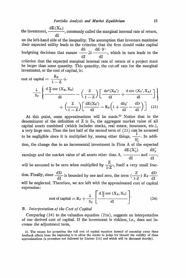
23 Pmtfolio Analysis and Market Equilibrium
dE(XA)the investment, ,commonly called the marginal internal rate of return,
dI on the left-hand side of the inequality. The assumption that investors maximize their expected utility leads to the criterion that the firm should make capital
dS dE-Fa budgeting decisions that ensure -3 , which in turn leads to the
d I d I criterion that the expected marginal internal rate of return of a project must be larger than some quantity. This quantity, the cut-off rate for the marginal investment, or the cost of capital, is:
RPcost of capital = --I-
1 -z
At this point, some approximations will be made.'Wotice that in the denominator of the definition of Z is ST, the aggregate market value of all capital assets combined (which includes stocks, real estate, insurance, etc.), a very large sum. Thus the last half of the second term of (23) can be assumed
to be negligible since it is multiplied by, among other things, -. In addi- s;
tion, the change due to an incremental investment in Firm A of the expected
will be assumed to be zero when multiplied by -, itself a very small frac-
earnings and the market value of all assets other than A, dE (Xh)
d I
dSk and ----,
dP z
1-z dD Z dD
tion. Finally, since -is bounded by one and zero, the term (-) RF-d I 1-Z dI
will be neglected. Therefore, we are left with the approximated cost of capital expression :
B. Interpretation of the Cost of Capital
Comparing (24) to the valuation equation (2 l a ) , suggests an interpretation of our derived cost of capital. If the investment is riskless, i.e., does not in- crease the adjustment term,
22. The reason for presenting the full cost of capital equation instead of assuming away these feedback effects from the beginning is to allow the reader to judge for himself the validity of these approximations (a procedure not followed by Lintner [I31 and which will be discussed shortly).
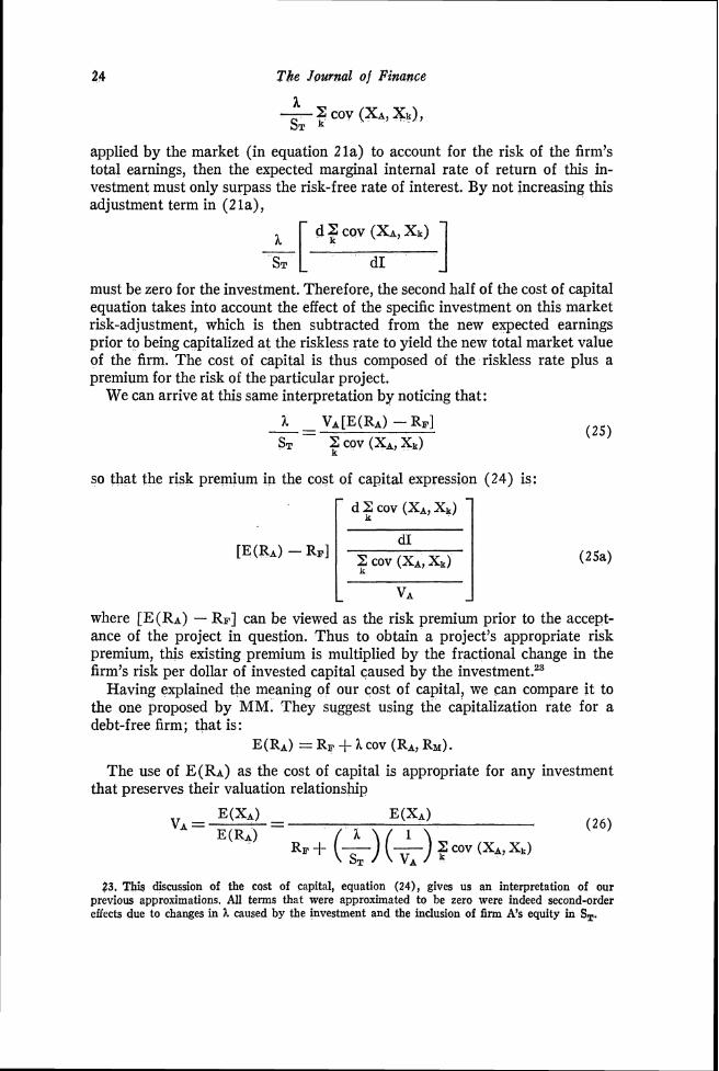
The Journal of Finance
applied by the market (in equation 21a) to account for the risk of the firm's total earnings, then the expected marginal internal rate of return of this in- vestment must only surpass the risk-free rate of interest. By not increasing this adjustment term in (21a),
d cov (XA, Xr)-[ IST d l
must be zero for the investment. Therefore, the second half of the cost of capital equation takes into account the effect of the specific investment on this market risk-adjustment, which is then subtracted from the new expected earnings prior to being capitalized a t the riskless rate to yield the new total market value of the firm. The cost of capital is thus composed of the riskless rate plus a premium for the risk of the particular project.
We can arrive a t this same interpretation by noticing that:
so that the risk premium in the cost of capital expression (24) is:
L where [E(RA) -RE] can be viewed as the risk premium prior to the accept- ance of the project in question. Thus to obtain a project's appropriate risk premium, this existing premium is multiplied by the fractional change in the firm's risk per dollar of invested capital caused by the in~estment. '~
Having explained the meaning of our cost of capital, we can compare i t to the one proposed by MM. They suggest using the capitalization rate for a debt-free firm; that is:
E(RA)=RF +A cov (RA, RM) . The use of E(Ra) as the cost of capital is appropriate for any investment
that preserves their valuation relationship
23. This discussion of the cost of capital, equation (24), gives us an interpretation of our previous approximations. All terms that were approximated to be zero were indeed second-order effects due to changes in h caused by the investment and the inclusion of firm A's equity in ST.
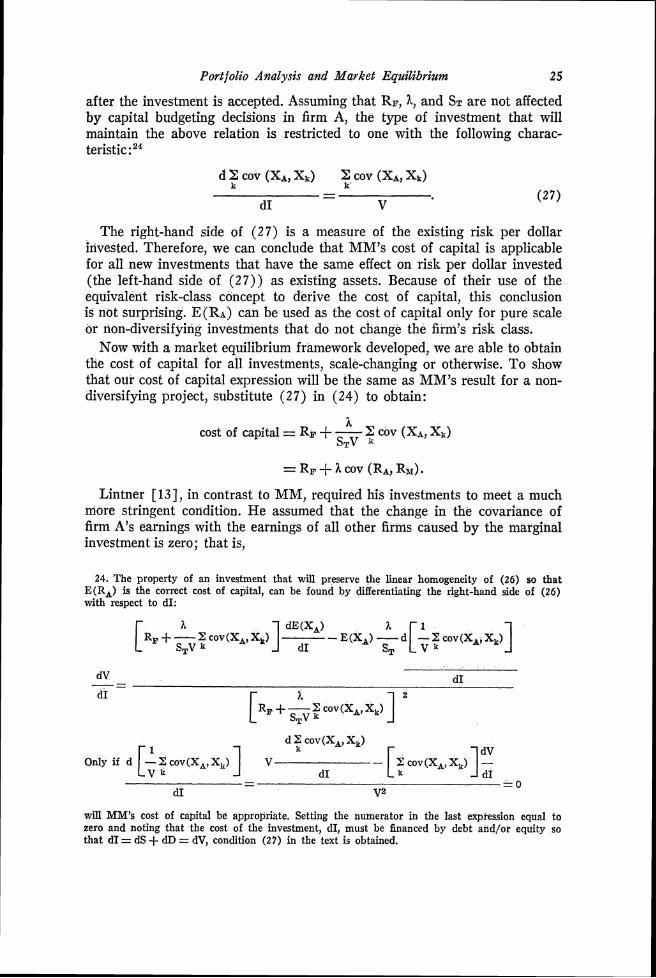
25 Portfolio Analysis and Market Equilibrium
after the investment is accepted. Assuming that RF, 1, and STare not affected by capital budgeting decisions in firm A, the type of investment that will maintain the above relation is restricted to one with the following charac-teristic: 24
d Z cov (XA,Xg) cov (XA,Xk)k -- ( 2 7 )
dI V
The right-hand side of (27) is a measure of the existing risk per dollar invested. Therefore, we can conclude that MM's cost of capital is applicable for all new investments that have the same effect on risk per dollar invested (the left-hand side of ( 2 7 ) ) as existing assets. Because of their use of the equivalent risk-class concept to derive the cost of capital, this conclusion is not surprising. E(Ra) can be used as the cost of capital only for pure scale or non-diversifying investments that do not change the firm's risk class.
Now with a market equilibrium framework developed, we are able to obtain the cost of capital for all investments, scale-changing or otherwise. To show that our cost of capital expression will be the same as MM's result for a non-diversifying project, substitute (27) in (24) to obtain:
h cost of capital =RF f- cov (XA,Xk)
STV
Lintner [13], in contrast to MM, required his investments to meet a much more stringent condition. He assumed that the change in the covariance of firm A's earnings with the earnings of all other firms caused by the marginal investment is zero; that is,
24. The property of an investment that will preserve the linear homogeneity of (26) so that E(RA) is the correct cost of capital, can be found by differentiating the right-hand side of (26) with respect to dI:
will MM's cost of capital be appropriate. Setting the numerator in the last expression equal to zero and noting that the cost of the investment, dI, must be financed by debt and/or equity so that d I =dS + dD = dV, condition (27) in the text is obtained.
The Journal of Finance
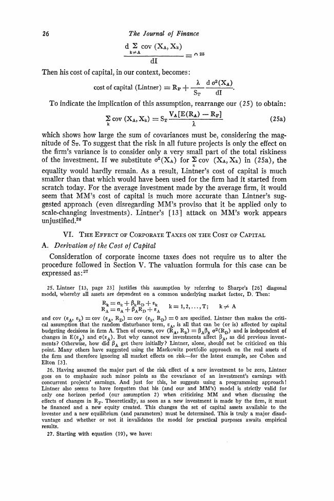
Then his cost of capital, in our context, becomes :
cost of capital (Lintner) =RE+-a a ST dI
To indicate the implication of this assumption, rearrange our (25) to obtain:
which shows how large the sum of covariances must be, considering the mag- nitude of ST.TOsuggest that the risk in all future projects is only the effect on the firm's variance is to consider only a very small part of the total riskiness of the investment. If we substitute 02(Xa) for 2 cov (XA,Xk) in (25a), the
equality would hardly remain. As a result, ~ in tne r ' s cost of capital is much smaller than that which would have been used for the firm had i t started from scratch today. For the average investment made by the average firm, it would seem that MM's cost of capital is much more accurate than Lintner's sug-gested approach (even disregarding MM's proviso that it be applied only to scale-changing investments). Lintner's [13] attack on MM's work appears u n j u ~ t i f i e d . ~ ~
VI. THEEFFECT TAXESOF CORPORATE ON THE COSTOF CAPITAL
A. Derivation of the Cost of Capital
Consideration of corporate income taxes does not require us to alter the procedure followed in Section V. The valuation formula for this case can be expressed as :27
25. Lintner [13, page 233 justifies this assumption by referring to Sharpe's [26] diagonal model, whereby all assets are dependent on a common underlying market factor, D. Then:
and cov (cA, cB) = cov (cA, RD).= cov ( E ~ ,RD) =0 are specified. Lintner then makes the criti- cal assumption that the random disturbance term, E*, is all that can be (or is) affected by capital budgeting decisions in firm A. Then of course, cov (RA, R,,) = PAP,, a2(RD) and is independent of changes in E ( E ~ ) and a(EA). But why cannot new investments affect fig, as did previous invest- ments? Otherwise, how did PA get there initially? Lintner, alone, should not be criticized on this point. Many others have suggested using the Markowitz portfolio approach on the real assets of the firm and therefore ignoring all market effects on risk-for the latest example, see Cohen and Elton [31.
26. Having assumed the major part of the risk effect of a new investment to be zero, Lintner goes on to emphasize such minor points as the covariance of an investment's earnings with concurrent projects' earnings. And just for this, he suggests using a programming approach! Lintner also seems to have forgotten that his (and our and MM's) model is strictly valid for only one horizon period (our assumption 2) when criticizing M M and when discussing the effects of changes in RF. Theoretically, as soon as a new investment is made by the firm, it must be financed and a new equity created. This changes the set of capital assets available to the investor and a new equilibrium (and parameters) must be determined. This is truly a major disad- vantage and whether or not it invalidates the model for practical purposes awaits empirical results.
27. Starting with equation (19), we have:
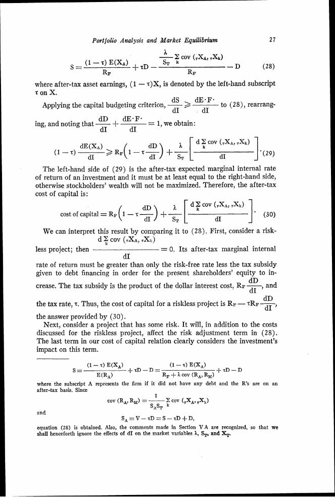
Portfolio Analysis and Market Equilibrium 2 7
where after-tax asset earnings, (1 -z)X, is denoted by the left-hand subscript z on X.
dS dE.F. Applying the capital budgeting criterion, -2 to (28)) rearrang-
dI dI
ing, and noting that -dD + dE.F. = 1, we obtain: d I dI
The left-hand side of (29) is the after-tax expected marginal internal rate of return of an investment and it must be at least equal to the right-hand side, otherwise stockholders' wealth will not be maximized. Therefore, the after-tax cost of capital is:
d cov ( J A , cost of capital= ..(I -.%) +&[ I. (30)d~
We can interpret this result by comparing it to (28). First, consider a risk- d :cov (TXA, TXlr)
less project; then = 0. Its after-tax marginal internal d I
rate of return must be greater than only the risk-free rate less the tax subsidy given to debt financing in order for the present shareholders' equity to in-
dD crease. The tax subsidy is the product of the dollar interest cost, RF -, and
d I dD
the tax rate, z. Thus, the cost of capital for a riskless project is R s -zRe -d I ' the answer provided by (30).
Next, consider a project that has some risk. I t will, in addition to the costs discussed for the riskless project, affect the risk adjustment term in (28). The last term in our cost of capital relation clearly considers the investment's impact on this term.
where the subscript A represents the firm if it did not have any debt and the R's are on an after-tax basis. Since
1 cov (R,, RM) = - cov (7XA~7Xk)
SAST and
S A = V - z D = S - z D + D ,
equation (28) is obtained. Also, the comments made in Section V A are recognized, so that we shall henceforth ignore the effects of d I on the market variables h, ST, and q.
28 The Journal of Finance
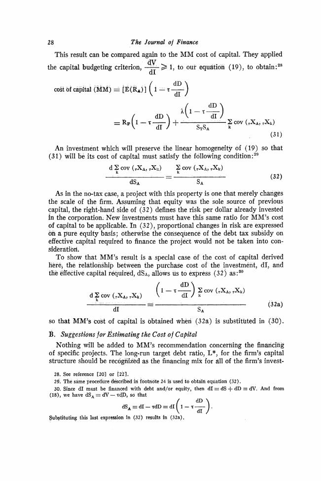
This result can be compared again to the MM cost of capital. They applied
the capital budgeting criterion, -dV 2 1, to our equation (19), to obtain:2sd I
cost bf capital (MM) = [E(R*) ] (1-z -3
An investment which will preserve the linear homogeneity of (19) so that (31) will be its cost of capital must satisfy the following c~ndi t ion: '~
d cov (Xi,TXIJ cov (&A, rXk)
~ S A --
Sa ( 3 2 )
As in the no-tax case, a project with this property is one that merely changes the scale of the firm. Assuming that equity was the sole source of previous capital, the right-hand side of (32) defines the risk per dollar already invested in the corporation. New investments must have this same ratio for MM's cost of capital to be applicable. In (32), proportional changes in risk are expressed on a pure equity basis; otherwise the consequence of the debt tax subsidy on effective capital required to finance the project would not be taken into con-sideratio&
To show that MM's result is a special case of the cost of capital derived here, the relationship between the purchase cost of the investment, dI, and the effectivecapital required, dSa, allows us to express (32) as:50
so that MM's cost of capital is obtained when (32a) is substituted in (30).
B. Suggestions for Estimating the Cost of Capital
Nothing will be added to MM's recommendation concerning the financing of specific projects. The long-run target debt ratio, L*, for the firm's capital structure should be reco&ized as the financing mix for all of the firm's invest-
28. See reference [20] or [22]. 29. The same procedure described in footnote 24 is used to obtain equation (32). 30. Since d I must be financed with debt and/or equity, then d I = dS f dD = dV. And from
(18), we have dSA = dV - zdD, so that
d S A = d I - ~ d D = d 1
Substituting this last expression in (32) results in (32a).
20 Portfotio Andysis and Market Bquilibriicm
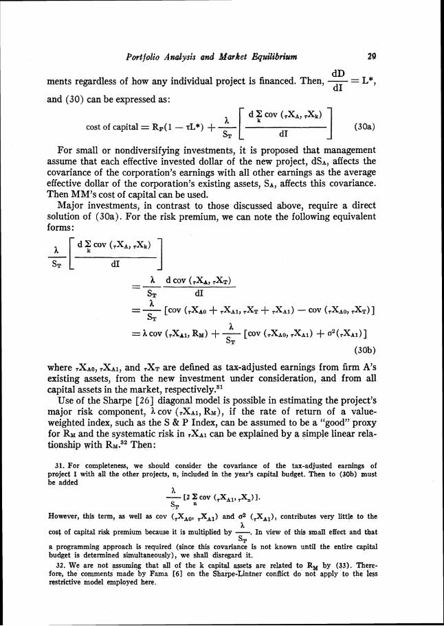
d D ments regardless of how any individual project is financed. Then, ---L*,
d I and (30) can be expressed as:
cost of capital = RF(l-TL*)+ - (30a)ST 1
For small or nondiversifying investments, it is proposed that management assume that each effective invested dollar of the new project, ~ S A ,affects the covariance of the corporation's earnings with all other earnings as the average effective dollar of the corporation's existing assets, SA,affects this covariance. Then MM's cost of capital can be used.
Major investments, in contrast to those discussed above, require a direct solution of (30a). For the risk premium, we can note the following equivalent forms:
where ~ X A O ,7 X ~ l ,and ~ X Tare defined as tax-adjusted earnings from firm A's existing assets, from the new investment under consideration, and from all capital assets in the market, re~pect ively .~~
Use of the Sharpe [26] diagonal model is possible in estimating the project's major risk component, hcov (,XAI, RM),if the rate of return of a value-weighted index, such as the S & P Index, can be assumed to be a "good" proxy for RMand the systematic risk in 7XAl can be explained by a simple linear rela-tionship with Then :
31. For completeness, we should consider the covariance of the tax-adjusted earnings of project 1 with all the other projects, n, included in the year's capital budget. Then to (30b) must be added
However, this term, as well as cov (,XAo, .XA1) and a2 (rXAl),contributes very little to the h
cost of capital risk premium because it is multiplied by -. In view of this small effect and that ST
a programming approach is required (since this covariance is not known until the entire capital budget is determined simultaneously), we shall disregard it.
32. We are not assuming that all of the k capital assets are related to Rw by (33) . There-fore, the comments made by Fama 161 on the Sharpe-Lintner conflict do not apply to the less restrictive model employed here.
30 The Journal of Finance
where a and b are parameters and E(E) = E ) 0. Applying (33) toCOV(RM, = the definition of the covariance, we have:
so that b and E(RM)are all that must be estimated.
VII. CONCLUSION
Two major issues of corporation finance, the financing and investment deci- sions of the firm, have been analyzed in this paper in the framework of the Sharpe-Lintner-Mossin market equilibrium capital asset pricing model, itself an extension of the Markowitz-Tobin portfolio model. The effects of the financing decision on aggregate equity values were the topics of Sections I11 and IV. The famous MM Propositions I and I1 were found to hold when put to the market equilibrium model, both in the no tax case (Section 111) and when corporate taxes were taken into account (Section IV). Thus the assump- tion of homogeneous risk-classes, constructed expressly to eliminate a full-blown market equilibrium model, and the arbitrage proof are no longer neces- sary. In place of arbitrage, a switching operation was discussed.
Sections V and VI were devoted to developing and interpreting the cost of capital, the minimum required rate of return individual projects within the firm must surpass in order that their shareholders not suffer a decrease in expected utility. MM's recommended cost of capital was found to be a special case (for nondiversifying investments) of the one developed here, albeit a most important special case. Then comparing Lintner's cost of capital to MM's, the latter version was thought to be more accurate in the majority of cases faced by the firm. Finally, cursory suggestions to estimate the cost of capital were made.
I t might be of interest to note that MM's discussions suggest an equilibrium portfolio model was implicitly being employed. For instance, they associated a rise in expected equity yields, when leverage increased, to an increased premium induced by the need to bear greater variability risk. And when dis- cussing their arbitrage operation, we can quote [ 2 1, footnote 111 :
In the language of the theory of choice, the exchanges are movements from inefficient points in the interior to efficient points on the boundary of the investor's opportunity set; and not movements between efficient points along the boundary . . . .
That their propositions are shown to hold in the portfolio model under market equilibrium conditions a decade later (and slightly earlier for Proposi- tion I in the time-state preference framework) should be regarded as a tribute to their partial equilibrium concept of the homogeneous risk-class.
But a word of caution is necessary in conclusion. We opened the analytical part of this paper with an enumeration of the assumptions. The results pre- sented here are conditional on these assumptions not grossly violating reality.

Portfolio Andysis and Market Equilibrium 3 1
REFERENCES
K. J. Arrow. "The Role of Securities in the Optimal Allocation of Risk-Bearing," Review o f Economic Studies, April, 1964.
G. Bierwag and M. Grove. "On Capital Asset Prices: Comment," Journal o f Finance, (March, 1965), pp. 89-93.
K. Cohen and E. Elton. 'LInter-temporal Portfolio Analysis Based on Simulation of Joint Returns," Management Science, (Sept., 1967), pp. 5-18.
G. Debreu. Theory of Value. New York: John Wiley and Sons, 1959. Chap. 7. E . Fama. [[Risk, Return and General Equilibrium in a Stable Paretian Market." Unpublished
manuscript, June, 1967. . "Risk, Return and General Equilibrium: Some Clarifying Comments." Journal
o f Finance, (March, 1968), pp. 29-40. I. Fisher. The Theory o f Interest. New York: Macmillan, 1930. Reprinted, Augustus M.
Kelley, 1961. J. Hirshleifer. "Efficient Allocation of Capital in an Uncertain World," American Economic
Review (May, 1964), pp. 77-85. . "Investment Decision Under Uncertainty: Choice-Theoretic Approaches," The
Quarterly Journal of Economics (November, 1965), pp. 509-536. . "Investment Decision Under Uncertainty: Applications of the State-Preference
Approach," The Quarterly Journal o f Economics (May, 1966), pp. 252-277. J. Lintner. "The Cost of Capital and Optimal Financing of Corporate Growth," Journal of
Finance, (May, 1963), pp. 292-310. . "Optimal Dividends and Corporate Growth Under Uncertainty," Quarterly
Jotwnal o f Economics, (February, 1964), pp. 49-95. . '[The Valuation of Risk Assets and The Selection of Risky Investments in
Stock Portfolios and Capital Budgets," Review of Economics and Statistics (February, 1965) pp. 13-37.
, "Security Prices, Risk, and Maximal Gains from Diversification," Journal of Finance (December, 1965), pp. 587-615.
J. Magee. "Decision Trees for Decision Making," Harvard Business Review, (July-August 1964), pp. 126-138.
H. Markowitz. "Portfolio Selection," Journal o f Finance, (March, 1952), pp. 77-91. , Portfolio Selection: Eficient Diversification of Investments. New York: John
Wiley and Sons, Inc., 1959. M. Miller. "Discussion," Journal o f Finance, (May, 1963), pp. 313-316. M. Miller and F. Modigliani. "Dividend Policy, Growth, and the Valuation of Shares,"
Journal of Business, (October, 1961), pp. 411-433. . "Some Estimates of the Cost of Capital to the Electric Utility Industry,
1954-57," American Economic Review (June, 1966), pp. 333-391. Modigliani and Miller. "The Cost of Capital, Corporation Finance and the Theory of In-
vestment," American Economic Review (June, 1958), pp. 261-97. . "Corporate Income Taxes and the Cost of Capital: A Correction," American
Economic Review (June, 1963), pp. 433-443. J. Mossin. "Equilibrium in a Capital Asset Market," Econometrica, (October, 1966), pp. 768-
783. A. Roy. "Safety First and the Holding of Assets," Econometrica (July, 1952), pp. 431-449. W. Sharpe. "Capital Asset Prices: A Theory of Market Equilibrium under Conditions of
Risk," Journal of Finance (September, 1964), pp. 425-442. . "A Simplified Model for Portfolio Analysis," Management Science (January,
1963), pp. 277-293. J. Tobin. "Liquidity Preference as Behavior Towards Risk," Review of Economic Studies
(February, 1958), pp. 65-86.
Recommended