INTERNATIONAL JOURNAL OF CLIMATOLOGYInt. J. Climatol. (2008)Published online in Wiley InterScience(www.interscience.wiley.com) DOI: 10.1002/joc.1688
Physiographically sensitive mapping of climatologicaltemperature and precipitation across the conterminous
United States
Christopher Daly,a* Michael Halbleib,a Joseph I. Smith,a Wayne P. Gibson,a
Matthew K. Doggett,a George H. Taylor,a Jan Curtisb and Phillip P. Pasterisb
a Oregon State University, Corvallis, OR 97331, USAb USDA Natural Resources Conservation Service Water and Climate Center, Portland, OR 97232, USA
ABSTRACT: Spatial climate data sets of 1971–2000 mean monthly precipitation and minimum and maximum temperaturewere developed for the conterminous United States. These 30-arcsec (∼800-m) grids are the official spatial climate datasets of the U.S. Department of Agriculture. The PRISM (Parameter-elevation Relationships on Independent Slopes Model)interpolation method was used to develop data sets that reflected, as closely as possible, the current state of knowledge ofspatial climate patterns in the United States. PRISM calculates a climate–elevation regression for each digital elevationmodel (DEM) grid cell, and stations entering the regression are assigned weights based primarily on the physiographicsimilarity of the station to the grid cell. Factors considered are location, elevation, coastal proximity, topographic facetorientation, vertical atmospheric layer, topographic position, and orographic effectiveness of the terrain. Surface stationsused in the analysis numbered nearly 13 000 for precipitation and 10 000 for temperature. Station data were spatially qualitycontrolled, and short-period-of-record averages adjusted to better reflect the 1971–2000 period.
PRISM interpolation uncertainties were estimated with cross-validation (C-V) mean absolute error (MAE) and the 70%prediction interval of the climate–elevation regression function. The two measures were not well correlated at the pointlevel, but were similar when averaged over large regions. The PRISM data set was compared with the WorldClim andDaymet spatial climate data sets. The comparison demonstrated that using a relatively dense station data set and thephysiographically sensitive PRISM interpolation process resulted in substantially improved climate grids over those ofWorldClim and Daymet. The improvement varied, however, depending on the complexity of the region. Mountainous andcoastal areas of the western United States, characterized by sparse data coverage, large elevation gradients, rain shadows,inversions, cold air drainage, and coastal effects, showed the greatest improvement. The PRISM data set benefited from apeer review procedure that incorporated local knowledge and data into the development process. Copyright 2008 RoyalMeteorological Society
KEY WORDS physiography; spatial climate; PRISM; interpolation; temperature; precipitation; rain shadow; cold air drainage;temperature inversion; coastal proximity; elevation; Daymet; WorldClim
Received 11 June 2007; Revised 27 December 2007; Accepted 28 December 2007
1. Introduction
Spatial climate data sets in digital form are currently ingreat demand. The most commonly used spatial climatedata sets are gridded estimates of mean daily minimumand maximum temperature and total precipitation on amonthly time step, averaged over a nominal 30-yearperiod. The demand for these data sets has been fueledin part by the linking of geographic information systems(GIS) to a variety of models and decision support tools,such as those used in agriculture, engineering, hydrology,ecology, and natural resource conservation.
Spatial climate data are often key drivers of computermodels and statistical analyses, which form the basis forscientific conclusions, management decisions, and other
* Correspondence to: Christopher Daly, PRISM Group, Department ofGeosciences, 2000 Kelley Engineering Center, Oregon State Univer-sity, Corvallis, OR 97331, USA. E-mail: [email protected]
important outcomes. It is therefore imperative that thesedata sets provide a realistic representation of the majorforcing factors that affect spatial climate patterns. Toachieve this high level of realism, methods used to createthe data sets must explicitly account for these factors.A detailed discussion of these factors is given in Daly(2006), and a brief overview is provided here.
General circulation patterns are largely responsible forlarge-scale climate variations, and include the positionsof storm tracks, prevailing wind directions, monsoonalcirculations, and other defining features of a region’sclimate. It is assumed that most of these patterns occurat scales large enough to be adequately reflected in thestation data, and therefore are not explicitly accountedfor by interpolation methods. Physiographic features onthe earth’s surface, namely water bodies and terrain,modulate these large-scale climate patterns. Water bodiesprovide moisture sources for precipitation, and create
Copyright 2008 Royal Meteorological Society

C. DALY ET AL.
complex temperature gradients along coastlines and inadjacent inland areas. Terrain effects include the directeffect of altitude on climate conditions, the blockage anduplift of major flow patterns by terrain barriers, and coldair drainage and pooling in valleys and depressions.
The relationship between elevation and precipitationis highly variable, but precipitation generally increaseswith elevation (Oke, 1978; Barry and Chorley, 1987).Exceptions are when terrain rises above the heightof a moist boundary layer or trade wind inversion(Mendonca and Iwaoka, 1969). Blocking and upliftingof moisture-bearing winds amplifies precipitation onwindward slopes, especially those with steep windwardinclines, and can sharply decrease it on leeward slopesdownwind, producing rain shadows (Smith, 1979; Dalyet al., 1994, 2002).
Temperature exhibits a strong, predictable decreasewith elevation when the atmosphere is well mixed, suchas occurs on summer days in inland areas (e.g. Willmottand Matsuura, 1995). The main summer exception is incoastal regions with well-defined marine layers, wheremaximum temperatures often increase with elevationabove the marine inversion. Winter temperatures, andminimum temperatures in all seasons, have a morecomplex relationship with elevation. In the absence ofsolar heating or significant winds to mix the atmosphere,temperatures stratify quickly, and cool, dense air drainsinto local valleys and depressions to form pools thatcan be hundreds of metres thick (Geiger, 1964; Hocevarand Martsolf, 1971; Bootsma, 1976; Gustavsson et al.,1998; Lindkvist et al., 2000; Daly et al., 2003). Thisresults in temperature inversions, in which temperaturesharply increases, rather than decreases, with elevation(Clements et al., 2003). In Polar regions, widespreadregional inversions hundreds of kilometres in extentcan dominate wintertime temperature patterns (Milewskaet al., 2005; Simpson et al., 2005). Terrain can also serveas a barrier between air masses, creating sharply definedhorizontal temperature gradients.
Coastal effects on temperature are most noticeablein situations where the water temperature is significantlydifferent from the adjacent land temperature (Haugen andBrown, 1980; Atkinson and Gajewski, 2002). Along theCalifornia coastline during summer, the contrast betweenthe cool Pacific Ocean and the adjacent warm land masscan create daytime air temperature gradients of more than10 °C in just a few kilometres across the coastal strip(Daly et al., 2002).
The above factors are most important at scales fromless than 1 km to 50 km or more (Daly, 2006). Severaladditional spatial climate-forcing factors are most impor-tant at relatively small scales of less than 1 km, but canhave influences at larger scales as well. These factorsinclude slope and aspect (McCutchan and Fox, 1986;Barry, 1992; Bolstad et al., 1998; Lookingbill and Urban,2003; Daly et al., 2007), riparian zones (Brosofske et al.,1997; Dong et al., 1998; Lookingbill and Urban, 2003),and land use/landcover (Davey and Pielke, 2005). Landuse/landcover variations are a major consideration in the
spatial representativeness of climate stations at muchlarger scales. For example, stations located near park-ing lots, buildings, or other heat-absorbing surfaces mayhave very different temperature regimes than those inopen grasslands or heavily vegetated areas (Davey andPielke, 2005). In data-sparse regions, a single station, andits particular land use/landcover regime, may influencethe interpolated climate conditions for tens of kilometresaround that station.
This paper describes the development of spatial climatedata sets of 1971–2000 mean monthly total precipitationand daily minimum and maximum temperature across theconterminous United States, using methods that striveto account for the major physiographic factors influ-encing climate patterns at scales of 1 km and greater.These data sets, created at 30-arcsec (∼800-m) grid res-olution, were commissioned by the U.S. Department ofAgriculture through the Natural Resources ConservationService (USDA-NRCS) to serve as the official spatialclimate data sets of the USDA. They are updates of the2.5-arcmin (∼4-km) 1961–1990 spatial climate data setsdeveloped in the 1990s (USDA-NRCS, 1998). The newdata sets were interpolated using the latest version of theParameter-elevation Regressions on Independent SlopesModel (PRISM) climate mapping system. Section 2 ofthis paper describes the study area and the digital eleva-tion model (DEM) used. In Section 3, the preparation ofstation data is described. Section 4 provides an overviewof the PRISM climate mapping system for this applica-tion, and summarizes the modelling, review, and revisionprocess. Section 5 presents the resulting gridded data sets,discusses model performance, and compares and con-trasts the PRISM data sets to two other spatial climatedata sets. Concluding remarks are given in Section 6.
2. Study area and digital elevation model
Climate data sets were developed at 30-arcsec resolutionin geographic (lat./long.) coordinates. A 30-arcsec gridcell is approximately 900 × 700 m at 40°N latitude, andis referred to as ‘800 m’ after the discussion of the eleva-tion grid in the next section. The boundaries of the gridwere 22 and 50°N and 65 and 125 °W. Memory, CPU, andmodel parameterization considerations required that inter-polation be performed separately in three regions: west-ern, central, and eastern United States, and the resultinggrids merged to form a complete conterminous U.S. grid.
Care was taken to include as many islands offshorethe U.S. mainland as possible, but undoubtedly somevery small islands were missed. To accommodate GISshoreline data sets of varying quality and resolution,the modelling region was extended offshore severalkilometres and generalized to include bays and inlets(Table I). However, the gridded climate estimates arevalid over land areas only.
The DEM was the single most important grid input tothe interpolation; it provided the independent variable forthe PRISM elevation regression function and served as
Copyright 2008 Royal Meteorological Society Int. J. Climatol. (2008)DOI: 10.1002/joc
PHYSIOGRAPHICALLY SENSITIVE MAPPING OF CLIMATOLOGICAL TEMPERATURE AND PRECIPITATION
Table I. Methods for preparation of PRISM input grids, part 1.
Modelinputgrid
Description Climateelement/region
Units Step Startinggrid
Operation
U.S. boundary andactual coastlinemask
Mask ofconterminous U.S.boundaries andcoastlines
All/All Binary (1 or0)
– U.S. boundaryvector file
Convert vectors torasters
Generalizedcoastlineand modeling mask
Mask for modellingregion, generalizedcoastlines
All/All Binary (1 or0)
– U.S. boundary andactual coastlinemask
Grow maskbeyond U.S.boundaries; fill inbays and inlets
Coastal proximityTCE
Distance fromcoastline, with baysand inlets treated astransition areas
Max and mintemp, centraland eastern US
Kilometres(0–50)
1 US boundary mask Distance fromcoastlines
2 Modelling mask Distance fromcoastlines
3 Steps 1 and 2grids
Average the twogrids
Coastal proximityTW
Index of marinepenetration throughcomplex terrain
Max and mintemp, westernUS
Index(0–1000)
1 US boundarymask and 800-mtemperature DEM
Coastal advectionmodel (Daly et al.,2003)
2 Generalizedcoastline mask
Coastal advectionmodel (Daly et al.,2003)
3 Steps 1 and 2grids
Step 3 =0.75(Step 1) +0.25 (Step 2)
Coastal proximityPCE
Distance fromgeneralized coastline
Precip, centraland eastern US
Kilometres(0–90)
– Modelling mask Distance fromcoastlines
Coastal proximityPW
Moisture index Precip, westernUS
Index(0–1000)
– Modelling maskand 800 mprecipitation DEM
Coastal trajectorymodel (Daly et al.,2003)
the basis for most of the other physiographic input gridsto PRISM (Section 4). The DEM used in this study wasderived from the 3-arcsec (∼80-m) National ElevationDatabase (NED) (NED; http://gisdata.usgs.gov/NED/).The NED elevation data was found to be superior toother DEMs for the conterminous United States, such asGTOPO30, Digital Terrain Elevation Database (DTED),and Space Shuttle Radar Topography Mission (SRTM),for this application. The GTOPO30 and DTED DEMshad noticeable elevation breaks, or ‘seams’ along someof the original U.S.Geological Survey (USGS) quadboundaries. The SRTM DEM had numerous grid cellswith missing data in areas of steep terrain, and possessedsignificant ground clutter associated with low microwavesignal-to-noise ratios.
A 30-arcsec (∼800-m) version of the NED DEM wasderived from the 3-arcsec (∼80-m) NED DEM by apply-ing a modified Gaussian filter (Barnes, 1964). This fil-ter provides a truly circular averaging area (as opposedto a typical rectangular block, which causes distortionalong the diagonals) and weights the surrounding gridcells in a Gaussian, or normal, distribution with distance,which better preserves local detail at and around the cen-tral grid cell than does a uniformly weighted average.
This 30-arcsec (∼800-m) DEM was used for interpolat-ing maximum and minimum temperature. An additionalfiltering step was performed to obtain a DEM suitablefor precipitation interpolation. The Gaussian filter wasapplied to the 30-arcsec (∼800-m) DEM to filter out ter-rain features up to 3.75 arcmin (∼7 km) in extent, whileretaining the 30-arcsec (∼800-m) grid resolution. Thedirect effects of elevation on precipitation appear to bemost important at scales of 5–10 km or greater, owing toa number of mechanisms, including the advective natureof moisture-bearing airflow, the viscosity of the atmo-sphere, delays between initial uplift and subsequent rain-out, and the movement of air around terrain obstacles(Daley, 1991; Daly et al., 1994; Funk and Michaelsen,2004; Sharples et al., 2005). In this paper, the two DEMsare hereafter referred to as the temperature and precipi-tation DEMs (Table II).
3. Station data
3.1. Data sources
Data from surface stations, numbering nearly 13 000for precipitation and nearly 10 000 for minimum and
Copyright 2008 Royal Meteorological Society Int. J. Climatol. (2008)DOI: 10.1002/joc

C. DALY ET AL.Ta
ble
II.
Met
hods
for
prep
arat
ion
ofPR
ISM
inpu
tgr
ids,
part
2.
Mod
elin
put
grid
Des
crip
tion
Clim
ate
elem
ent
Uni
tsSt
epSt
artin
ggr
idO
pera
tion
Rad
ius
ofin
fluen
ce(k
m)
Cel
lw
eigh
ting
profi
le
800-
mTe
mpe
ratu
reD
EM
DE
Mfo
rte
mpe
ratu
rein
terp
olat
ion
Min
.an
dm
ax.
tem
pera
ture
m–
80-m
NE
DD
EM
Ave
rage
,an
dco
arse
nre
solu
tion
to80
0m
1.3
Gau
ssia
n(B
arne
s,19
64)
800-
mPr
ecip
itatio
nD
EM
DE
Mfo
rpr
ecip
itatio
nin
terp
olat
ion
Prec
ipita
tion
m–
800-
mTe
mpe
ratu
reD
EM
Ave
rage
7G
auss
ian
(Bar
nes,
1964
)To
pogr
aphi
cfa
cets
Are
asof
cons
iste
ntas
pect
Min
.an
dm
ax.
tem
p.,
prec
ipita
tion
Dir
ectio
non
eigh
tco
mpa
sspo
ints
180
0-m
Prec
ipita
tion
DE
MA
vera
ge0.
8,12
,24
,36
,48
,60
Gau
ssia
n(B
arne
s,19
64)
2St
ep1
grid
sFa
cet
(Gib
son
etal
.,19
97)
0.8,
12,
24,
36,
48,
60
Uni
form
Pote
ntia
lw
inte
rtim
ein
vers
ion
heig
htE
stim
ates
alti
tude
ofbo
unda
rybe
twee
nla
yer
1(b
ound
ary
laye
r)an
dla
yer
2(f
ree
atm
osph
ere)
Min
.te
mpe
ratu
real
lye
ar;
max
.te
mp.
inw
inte
r(N
ov–
Mar
)
m1
800-
mTe
mpe
ratu
reD
EM
Min
imum
19–
2St
ep1
grid
Ave
rage
44U
nifo
rm3
Step
2gr
idA
dd25
0m
––
Moi
stbo
unda
ryla
yer
heig
htE
stim
ates
altit
ude
ofbo
unda
rybe
twee
nla
yer
1(m
oist
boun
dary
laye
r)an
dla
yer
2(d
rier
atm
osph
ere
abov
e)
Prec
ip.
inw
este
rnU
Sm
1C
ount
ybo
unda
ries
Cou
ntie
sw
est
ofth
eC
asca
decr
est
inO
Ran
dW
Agi
ven
laye
r1
heig
htof
2200
m;
all
othe
rar
eas
4000
m
––
Topo
grap
hic
inde
xE
stim
ates
how
muc
hhi
gher
pixe
lis
than
surr
ound
ing
neig
hbou
rhoo
d
Min
.te
mp.
all
year
;m
ax.
tem
p.in
win
ter
(Nov
–M
ar)
m1
800-
mTe
mpe
ratu
reD
EM
Min
imum
14–
2St
ep1
grid
Ave
rage
15U
nifo
rm3
Step
2gr
idSu
btra
ctst
ep2
grid
from
DE
M–
–
Eff
ectiv
ete
rrai
nhe
ight
Est
imat
esor
ogra
phic
ally
effe
ctiv
epr
ofile
ofte
rrai
nfe
atur
es
Prec
ipita
tion
m1
800-
mPr
ecip
itatio
nD
EM
Min
imum
22–
2St
ep1
grid
Ave
rage
11U
nifo
rm3
Step
2gr
idSu
btra
ctst
ep2
grid
from
DE
M–
–
4St
ep3
grid
Ave
rage
15U
nifo
rm
Copyright 2008 Royal Meteorological Society Int. J. Climatol. (2008)DOI: 10.1002/joc
PHYSIOGRAPHICALLY SENSITIVE MAPPING OF CLIMATOLOGICAL TEMPERATURE AND PRECIPITATION
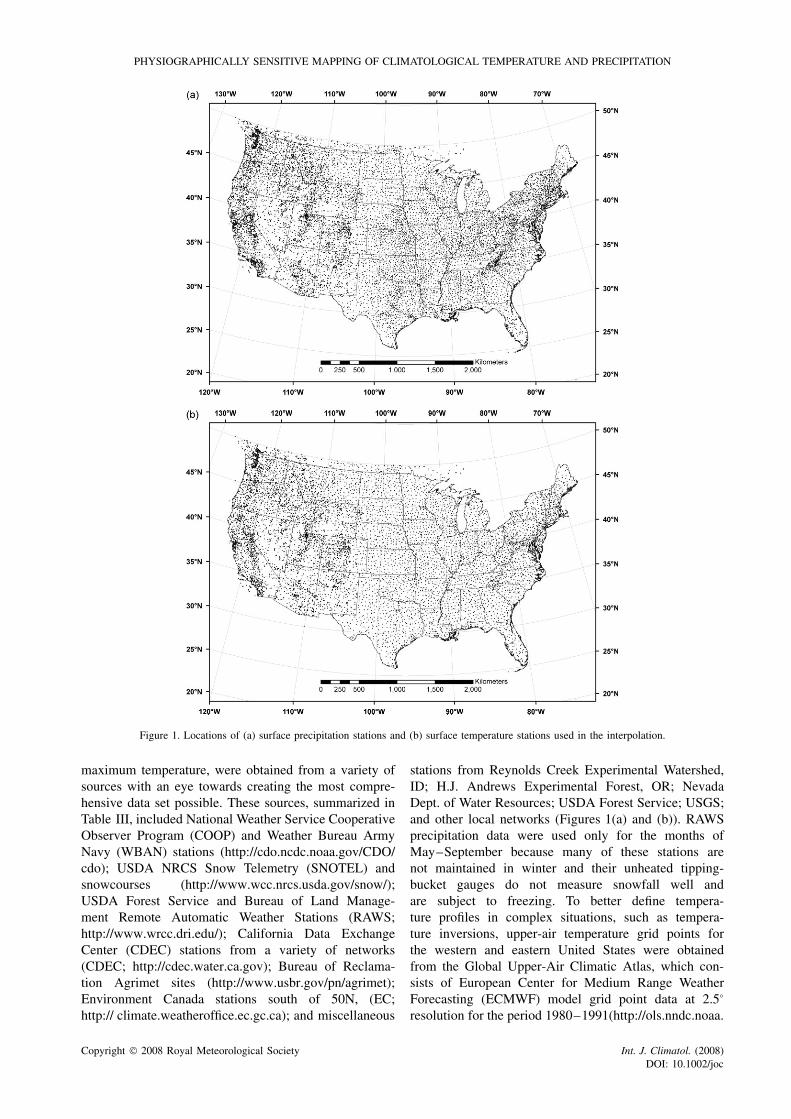
Figure 1. Locations of (a) surface precipitation stations and (b) surface temperature stations used in the interpolation.
maximum temperature, were obtained from a variety ofsources with an eye towards creating the most compre-hensive data set possible. These sources, summarized inTable III, included National Weather Service CooperativeObserver Program (COOP) and Weather Bureau ArmyNavy (WBAN) stations (http://cdo.ncdc.noaa.gov/CDO/cdo); USDA NRCS Snow Telemetry (SNOTEL) andsnowcourses (http://www.wcc.nrcs.usda.gov/snow/);USDA Forest Service and Bureau of Land Manage-ment Remote Automatic Weather Stations (RAWS;http://www.wrcc.dri.edu/); California Data ExchangeCenter (CDEC) stations from a variety of networks(CDEC; http://cdec.water.ca.gov); Bureau of Reclama-tion Agrimet sites (http://www.usbr.gov/pn/agrimet);Environment Canada stations south of 50N, (EC;http:// climate.weatheroffice.ec.gc.ca); and miscellaneous
stations from Reynolds Creek Experimental Watershed,ID; H.J. Andrews Experimental Forest, OR; NevadaDept. of Water Resources; USDA Forest Service; USGS;and other local networks (Figures 1(a) and (b)). RAWSprecipitation data were used only for the months ofMay–September because many of these stations arenot maintained in winter and their unheated tipping-bucket gauges do not measure snowfall well andare subject to freezing. To better define tempera-ture profiles in complex situations, such as tempera-ture inversions, upper-air temperature grid points forthe western and eastern United States were obtainedfrom the Global Upper-Air Climatic Atlas, which con-sists of European Center for Medium Range WeatherForecasting (ECMWF) model grid point data at 2.5°
resolution for the period 1980–1991(http://ols.nndc.noaa.
Copyright 2008 Royal Meteorological Society Int. J. Climatol. (2008)DOI: 10.1002/joc
C. DALY ET AL.
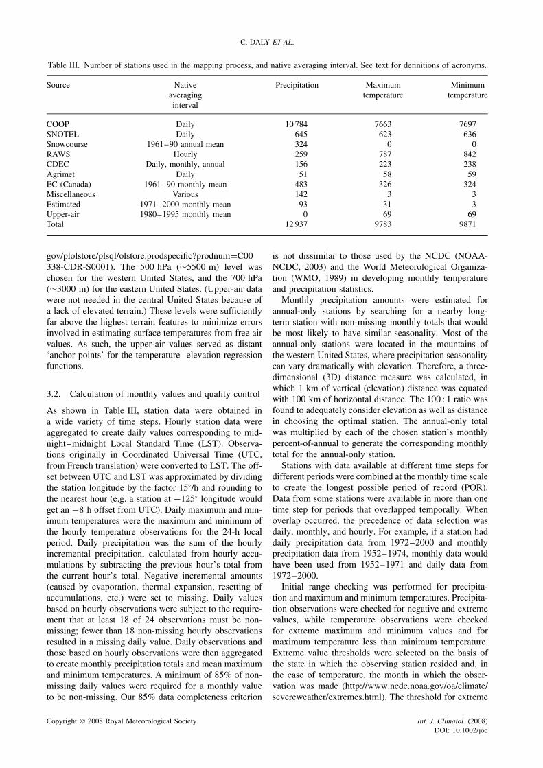
Table III. Number of stations used in the mapping process, and native averaging interval. See text for definitions of acronyms.
Source Nativeaveraginginterval
Precipitation Maximumtemperature
Minimumtemperature
COOP Daily 10 784 7663 7697SNOTEL Daily 645 623 636Snowcourse 1961–90 annual mean 324 0 0RAWS Hourly 259 787 842CDEC Daily, monthly, annual 156 223 238Agrimet Daily 51 58 59EC (Canada) 1961–90 monthly mean 483 326 324Miscellaneous Various 142 3 3Estimated 1971–2000 monthly mean 93 31 3Upper-air 1980–1995 monthly mean 0 69 69Total 12 937 9783 9871
gov/plolstore/plsql/olstore.prodspecific?prodnum=C00338-CDR-S0001). The 500 hPa (∼5500 m) level waschosen for the western United States, and the 700 hPa(∼3000 m) for the eastern United States. (Upper-air datawere not needed in the central United States because ofa lack of elevated terrain.) These levels were sufficientlyfar above the highest terrain features to minimize errorsinvolved in estimating surface temperatures from free airvalues. As such, the upper-air values served as distant‘anchor points’ for the temperature–elevation regressionfunctions.
3.2. Calculation of monthly values and quality control
As shown in Table III, station data were obtained ina wide variety of time steps. Hourly station data wereaggregated to create daily values corresponding to mid-night–midnight Local Standard Time (LST). Observa-tions originally in Coordinated Universal Time (UTC,from French translation) were converted to LST. The off-set between UTC and LST was approximated by dividingthe station longitude by the factor 15°/h and rounding tothe nearest hour (e.g. a station at −125° longitude wouldget an −8 h offset from UTC). Daily maximum and min-imum temperatures were the maximum and minimum ofthe hourly temperature observations for the 24-h localperiod. Daily precipitation was the sum of the hourlyincremental precipitation, calculated from hourly accu-mulations by subtracting the previous hour’s total fromthe current hour’s total. Negative incremental amounts(caused by evaporation, thermal expansion, resetting ofaccumulations, etc.) were set to missing. Daily valuesbased on hourly observations were subject to the require-ment that at least 18 of 24 observations must be non-missing; fewer than 18 non-missing hourly observationsresulted in a missing daily value. Daily observations andthose based on hourly observations were then aggregatedto create monthly precipitation totals and mean maximumand minimum temperatures. A minimum of 85% of non-missing daily values were required for a monthly valueto be non-missing. Our 85% data completeness criterion
is not dissimilar to those used by the NCDC (NOAA-NCDC, 2003) and the World Meteorological Organiza-tion (WMO, 1989) in developing monthly temperatureand precipitation statistics.
Monthly precipitation amounts were estimated forannual-only stations by searching for a nearby long-term station with non-missing monthly totals that wouldbe most likely to have similar seasonality. Most of theannual-only stations were located in the mountains ofthe western United States, where precipitation seasonalitycan vary dramatically with elevation. Therefore, a three-dimensional (3D) distance measure was calculated, inwhich 1 km of vertical (elevation) distance was equatedwith 100 km of horizontal distance. The 100 : 1 ratio wasfound to adequately consider elevation as well as distancein choosing the optimal station. The annual-only totalwas multiplied by each of the chosen station’s monthlypercent-of-annual to generate the corresponding monthlytotal for the annual-only station.
Stations with data available at different time steps fordifferent periods were combined at the monthly time scaleto create the longest possible period of record (POR).Data from some stations were available in more than onetime step for periods that overlapped temporally. Whenoverlap occurred, the precedence of data selection wasdaily, monthly, and hourly. For example, if a station haddaily precipitation data from 1972–2000 and monthlyprecipitation data from 1952–1974, monthly data wouldhave been used from 1952–1971 and daily data from1972–2000.
Initial range checking was performed for precipita-tion and maximum and minimum temperatures. Precipita-tion observations were checked for negative and extremevalues, while temperature observations were checkedfor extreme maximum and minimum values and formaximum temperature less than minimum temperature.Extreme value thresholds were selected on the basis ofthe state in which the observing station resided and, inthe case of temperature, the month in which the obser-vation was made (http://www.ncdc.noaa.gov/oa/climate/severeweather/extremes.html). The threshold for extreme
Copyright 2008 Royal Meteorological Society Int. J. Climatol. (2008)DOI: 10.1002/joc
PHYSIOGRAPHICALLY SENSITIVE MAPPING OF CLIMATOLOGICAL TEMPERATURE AND PRECIPITATION
precipitation was chosen to be 115% of the state record24-h precipitation. The threshold for extreme maximumtemperature was chosen to be 3 °C above the statemonthly record maximum temperature. Likewise, thethreshold for extreme minimum temperature was chosento be 3 °C below the state monthly recorded minimumtemperature. The additional allowances were to accom-modate potential new records.
Daily precipitation observations and hourly incremen-tal amounts derived from accumulation observations weresubject to both negative and extreme value checks, whilemonthly precipitation observations were checked for neg-ative values only. Monthly and daily maximum and min-imum temperatures, as well as hourly air temperatures,were subject to maximum and minimum temperatureextreme checks. Observations that failed any of the abovetests were set to missing.
Station elevations were checked for consistency against800-m DEM elevations at the given station locations.Elevation discrepancies of more than 200 m were inves-tigated, and either the station location or elevation cor-rected as a result.
Several spatial quality control (QC) procedures wereconducted on the monthly data. In an initial QC screeningstep, monthly averages for 1971–2000 were calculatedfor stations having data during this time period. Stationsnot having data during 1971–2000 had historical aver-ages calculated from their entire POR. These averageswere tested for spatial consistency using the ASSAY QCsystem, a version of PRISM that estimates data for spe-cific station locations and compares them to the observedvalues (Daly et al., 2000; Gibson et al., 2002). Averagesfailing the ASSAY QC check were immediately omit-ted from further consideration if (1) they were RAWSor CDEC stations, (2) they had less than three years ofhistorical data, or (3) had three or more years of histor-ical data but had fewer than four consecutive months ofnon-missing data during those years. These stations wereconsidered to be at highest risk for poor quality.
In the second spatial QC step, all individual monthlyvalues from the remaining stations were tested for spatialconsistency using the ASSAY QC system; values failingthis test were set to missing. The remaining monthlyvalues were averaged and subjected to adjustment, ifneeded, as described in Appendix A.
In the third spatial QC step, all SNOTEL temperaturedata were subjected to a recently developed spatial QCsystem for temperature data from this network. Detailson the operation of this system are available in Dalyet al. (2005). Temperature data subjected to this QCprocess were first passed through the aforementionedrange checks. SNOTEL temperature data were also testedfor extended periods of unchanging values (flatliners);temperatures remaining unchanged (less than 0.1 °C dailydifference) for longer than ten consecutive days were setto missing. In addition, temperature values remaining atexactly 0.0 °C for two or more consecutive days (which isa known problem in SNOTEL data) were set to missing.
3.3. Period-of-record adjustment
Monthly station data passing the above QC tests wereaveraged to create 1971–2000 monthly means. A1971–2000 monthly mean calculated using data from atleast 23 of these 30 years (75% data coverage) was con-sidered to be sufficiently characteristic of the 1971–2000period, and was termed a ‘long-term’ station. However,many stations had a POR with fewer than 23 years. Itwas advantageous to include these ‘short-term’ stationsin the analysis because they often added information tothe interpolation process at critical locations. In orderto minimize temporal biases from these short-term sta-tions, their POR means were adjusted to the 1971–2000period. The assessment and adjustment of averages wasperformed for each month individually; therefore, it waspossible for a station to be considered long term for somemonths and short term for others. A discussion of theadjustment process is given in Appendix A.
4. PRISM overview and modelling
PRISM (Daly et al., 1994, 2001, 2002, 2003; Daly, 2006)is a knowledge-based system developed primarily tointerpolate climate elements in physiographically com-plex landscapes. The regression-based PRISM uses pointdata, a DEM, other spatial data sets, and an encodedspatial climate knowledge base to generate estimates ofannual, monthly, daily, and event-based climatic ele-ments. These estimates are interpolated to a regular grid,making them GIS-compatible. Previous mapping effortswith PRISM have included peer-reviewed, official USDAprecipitation and temperature maps for all 50 states andCaribbean and Pacific Islands; a new official climateatlas for the United States; a 112-year series of monthlytemperature, precipitation, and dew point maps for theconterminous 48 states; detailed precipitation and tem-perature maps for Canada, China, and Mongolia, and thefirst comprehensive precipitation maps for the EuropeanAlps region (Daly et al., 2001; Hannaway et al., 2005;Milewska et al., 2005; Schwarb et al., 2001a,b; Simpsonet al., 2005). Reports and papers describing PRISM areavailable from http://prism.oregonstate.edu.
4.1. The climate–elevation regression function
PRISM adopts the assumption that for a localized region,elevation is the most important factor in the distributionof temperature and precipitation (Daly et al., 2002).PRISM calculates a linear climate–elevation relationshipfor each DEM grid cell, but the slope of this line changeslocally with elevation (through elevation weighting) asdictated by the data points. Beyond the lowest or higheststation, the function can be extrapolated linearly as faras needed. A simple, rather than multiple, regressionmodel was chosen because controlling and interpretingthe complex relationships between multiple independentvariables and climate is difficult. Instead, weighting ofthe data points (discussed later) controls for the effectsof variables other than elevation.
Copyright 2008 Royal Meteorological Society Int. J. Climatol. (2008)DOI: 10.1002/joc
C. DALY ET AL.
The climate–elevation regression is developed from X,Y pairs of elevation and climate observations suppliedby station data. A moving-window procedure is used tocalculate a unique climate–elevation regression functionfor each grid cell. The simple linear regression has theform
Y = β1X + β0 (1)
where Y is the predicted climate element, β1 and β0 arethe regression slope and intercept, respectively, and X
is the DEM elevation at the target grid cell. The DEMelevation is represented at a spatial scale appropriatefor the climate element being mapped (discussed inSection 2).
4.2. Station weighting
Upon entering the regression function, each station isassigned a weight that is based on several factors. Thecombined weight (W ) of a station is given by thefollowing:
W = Wc[FdWd2 + FzWz
2]1/2Wp Wf Wl Wt We (2)
where Wc, Wd, Wz, Wp, Wf, Wl, Wt, and We are the clus-ter, distance, elevation, coastal proximity, topographicfacet, vertical layer, topographic position, and effectiveterrain weights, respectively, and Fd and Fz are user-specified distance and elevation weighting importancescalars (Daly et al., 2002; Daly et al., 2007). All weightsand importance factors, individually and combined, arenormalized to sum to unity. Table IV summarizes howthe PRISM elevation regression and station weightingfunctions account for the physiographic climate forcingfactors described in Section 1, and provide references forfurther information. The focus in the following discus-sions is on those station-weighting functions that havenot been previously published or have been updated forthe current application.
4.2.1. Cluster, distance, and elevation weighting
Cluster weighting seeks to limit the influence of stationsthat are clustered with other nearby stations, which canlead to over-representation in the regression function.A detailed discussion of cluster weight is provided inAppendix B.
A station is down-weighted when it is relatively distantfrom the target grid cell. The distance weight is given as
Wd ={ 1; d − rm ≤ 0
1(d − rm)a
; d − rm > 0
}(3)
where d is the horizontal distance between the stationand the target grid cell, a is the distance weightingexponent, and rm is the minimum radius of influence. Inthis application, a was set to 2, which is equivalent to aninverse-distance-squared weighting function, and rm wasset to approximately 7 km for precipitation and 10 kmfor temperature. The 7-km precipitation value matched
the estimated minimum scale at which elevation directlyaffects precipitation patterns (discussed in Section 1). The10-km temperature value represents the minimum scale ofthe effects of land use on station representativeness in thisapplication. Implementing this minimum radius reduced‘bull’s eyes’ and other artifacts created in the interpolatedtemperature fields caused by variations in station sitingand the surrounding land use/land cover. These effectsare not yet well understood, but can be highly significant(Mahmood et al., 2006).
A station is down-weighted when it is at a muchdifferent elevation than the target grid cell. A discussionof elevation weighting is given in Daly et al., (2002,Section 4.1).
4.2.2. Coastal proximity
Coastal proximity weighting is used to define gradientsin precipitation or temperature that may occur due toproximity to large water bodies (Daly et al., 2002, 2003).Stations with coastal proximities similar to that of thetarget grid cell are assigned relatively high weights inthe regression function.
For this application, coastal proximity guidance in thePRISM modelling run was provided through four coastalproximity grids, depending on the region and climateelement. In the central and eastern United States, thecoastal proximity grid for precipitation (abbreviated PCE)was composed simply of distances from the generalizedcoastline grid (Table I). A simple distance was adequatebecause of a lack of terrain features. The generalizedcoastline is used because bays and inlets were not con-sidered to be as important moisture sources as the openocean for precipitation. In the central and eastern UnitedStates, the coastal proximity grid for temperature (abbre-viated TCE) was a weighted average of the distancesfrom the actual and generalized coastlines, the ratio-nale being that bays and inlets experience a temperatureenvironment that is a transition between inland and fullyoceanic (Table I).
Complex terrain along the U.S. West Coast requiredmore sophisticated methods of estimating coastal proxim-ity. An advection model was designed to quantify coastalproximity for temperature mapping (abbreviated TW;Table I). The advection model is a cost–benefit algorithmthat assesses the optimal path a surface air parcel mighttake as it moves from the coast to each inland pixel. Thebasic assumption is that the mean coastal influence expe-rienced at a site will be the result of a flow path fromthe coast that minimizes two factors: (1) modification ofthe air by continental influences, which accumulates asthe path length over land increases (path length penalty);and (2) loss of momentum caused by flowing over terrainobstacles (terrain penalty). Predominant mesoscale flowpatterns, which aid certain flow paths and cause moreeffective inland penetration, are also accounted for bydecreasing the path length penalty for predominant direc-tions and increasing it for infrequent directions. For theWest Coast, flow paths from the west and northwest (typi-cal summertime directions) were set to incur substantially
Copyright 2008 Royal Meteorological Society Int. J. Climatol. (2008)DOI: 10.1002/joc

PHYSIOGRAPHICALLY SENSITIVE MAPPING OF CLIMATOLOGICAL TEMPERATURE AND PRECIPITATION
Tabl
eIV
.PR
ISM
algo
rith
ms
and
asso
ciat
edph
ysio
grap
hic
clim
ate
forc
ing
fact
ors,
inpu
tsto
the
algo
rith
ms,
and
refe
renc
eson
thei
rfo
rmul
atio
nan
dus
e.M
etho
dsus
edto
prep
are
the
grid
ded
mod
elin
puts
are
sum
mar
ized
inTa
bles
Ian
d2.
PRIS
Mal
gori
thm
Des
crip
tion
Phys
iogr
aphi
cfo
rcin
gfa
ctor
sIn
puts
toal
gori
thm
Ref
eren
ce
Ele
vatio
nre
gres
sion
func
tion
Dev
elop
slo
cal
rela
tions
hips
betw
een
clim
ate
and
elev
atio
nD
irec
tef
fect
sof
elev
atio
nSt
atio
nda
taD
EM
Thi
spa
per,
Sect
ion
4.1
Clu
ster
wei
ghtin
gD
ownw
eigh
tsst
atio
nscl
uste
red
with
othe
rs–
Stat
ion
loca
tions
and
elev
atio
nsT
his
pape
r,A
ppen
dix
B
Dis
tanc
ew
eigh
ting
Upw
eigh
tsst
atio
nsth
atar
eho
rizo
ntal
lycl
ose
Spat
ial
cohe
renc
eof
clim
ate
regi
mes
Stat
ion
loca
tions
Thi
spa
per,
Sect
ion
4.2.
1
Ele
vatio
nw
eigh
ting
Upw
eigh
tsst
atio
nsth
atar
eve
rtic
ally
clos
eD
irec
tef
fect
sof
elev
atio
nD
EM
Stat
ion
loca
tions
and
elev
atio
ns
Dal
yet
al.
(200
2),
Sect
ion
4.1
Topo
grap
hic
face
tw
eigh
ting
Upw
eigh
tsst
atio
nson
the
sam
esi
deof
ate
rrai
nba
rrie
r,or
onth
esa
me
expo
sure
,at
six
scal
es
Rai
nsh
adow
sA
irm
ass
sepa
ratio
nD
EM
Topo
grap
hic
face
tgr
ids
Stat
ion
loca
tions
Dal
yet
al.
(200
2),
Sect
ion
5
Coa
stal
prox
imity
wei
ghtin
gU
pwei
ghts
stat
ions
havi
ngsi
mila
rex
posu
reto
coas
tal
influ
ence
s
Eff
ects
ofw
ater
bodi
eson
tem
pera
ture
and
prec
ipita
tion
DE
MC
oast
alpr
oxim
itygr
idM
oist
ure
inde
xgr
idSt
atio
nlo
catio
ns
Dal
yet
al.
(200
2),
Sect
ion
6D
aly
etal
.(2
003)
,Se
ctio
ns2.
3.2
–2.
3.3
Two-
laye
rat
mos
pher
ew
eigh
ting
Ifan
inve
rsio
nis
pres
ent,
upw
eigh
tsst
atio
nsin
the
sam
eve
rtic
alla
yer
(bou
ndar
yla
yer
orfr
eeat
mos
pher
e)
Tem
pera
ture
inve
rsio
ns;
vert
ical
lim
itto
moi
stbo
unda
ryla
yer
(pre
cipi
tatio
n)
DE
MIn
vers
ion
heig
htgr
idSt
atio
nlo
catio
ns
Dal
yet
al.
(200
2),
Sect
ion
7D
aly
etal
.(2
003)
,Se
ctio
ns2.
3.2
–2.
3.4
Topo
grap
hic
posi
tion
wei
ghti
ngU
pwei
ghts
stat
ions
havi
ngsi
mil
arsu
scep
tibi
lity
toco
ldai
rpo
olin
g
Col
dai
rdr
aina
geD
EM
Topo
grap
hic
inde
xgr
idSt
atio
nlo
catio
ns
Dal
yet
al.
(200
7),
Sect
ion
4
Eff
ectiv
ete
rrai
nhe
ight
wei
ghti
ngM
odifi
esre
gres
sion
slop
eto
refle
ctab
ility
ofte
rrai
nto
affe
ctpr
ecip
itatio
npa
ttern
s;up
wei
ghts
stat
ions
onsi
mila
rte
rrai
n
Oro
grap
hic
effe
ctiv
enes
sof
terr
ain
feat
ures
DE
ME
ffec
tive
terr
ain
heig
htgr
idSt
atio
nlo
catio
ns
Thi
spa
per,
App
endi
xC
Copyright 2008 Royal Meteorological Society Int. J. Climatol. (2008)DOI: 10.1002/joc
C. DALY ET AL.
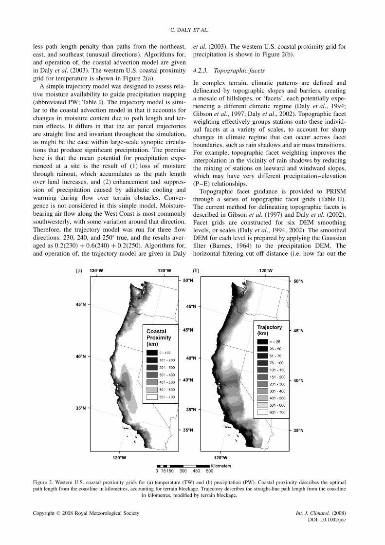
less path length penalty than paths from the northeast,east, and southeast (unusual directions). Algorithms for,and operation of, the coastal advection model are givenin Daly et al. (2003). The western U.S. coastal proximitygrid for temperature is shown in Figure 2(a).
A simple trajectory model was designed to assess rela-tive moisture availability to guide precipitation mapping(abbreviated PW; Table I). The trajectory model is simi-lar to the coastal advection model in that it accounts forchanges in moisture content due to path length and ter-rain effects. It differs in that the air parcel trajectoriesare straight line and invariant throughout the simulation,as might be the case within large-scale synoptic circula-tions that produce significant precipitation. The premisehere is that the mean potential for precipitation expe-rienced at a site is the result of (1) loss of moisturethrough rainout, which accumulates as the path lengthover land increases, and (2) enhancement and suppres-sion of precipitation caused by adiabatic cooling andwarming during flow over terrain obstacles. Conver-gence is not considered in this simple model. Moisture-bearing air flow along the West Coast is most commonlysouthwesterly, with some variation around that direction.Therefore, the trajectory model was run for three flowdirections: 230, 240, and 250° true, and the results aver-aged as 0.2(230) + 0.6(240) + 0.2(250). Algorithms for,and operation of, the trajectory model are given in Daly
et al. (2003). The western U.S. coastal proximity grid forprecipitation is shown in Figure 2(b).
4.2.3. Topographic facets
In complex terrain, climatic patterns are defined anddelineated by topographic slopes and barriers, creatinga mosaic of hillslopes, or ‘facets’, each potentially expe-riencing a different climatic regime (Daly et al., 1994;Gibson et al., 1997; Daly et al., 2002). Topographic facetweighting effectively groups stations onto these individ-ual facets at a variety of scales, to account for sharpchanges in climate regime that can occur across facetboundaries, such as rain shadows and air mass transitions.For example, topographic facet weighting improves theinterpolation in the vicinity of rain shadows by reducingthe mixing of stations on leeward and windward slopes,which may have very different precipitation–elevation(P–E) relationships.
Topographic facet guidance is provided to PRISMthrough a series of topographic facet grids (Table II).The current method for delineating topographic facets isdescribed in Gibson et al. (1997) and Daly et al. (2002).Facet grids are constructed for six DEM smoothinglevels, or scales (Daly et al., 1994, 2002). The smoothedDEM for each level is prepared by applying the Gaussianfilter (Barnes, 1964) to the precipitation DEM. Thehorizontal filtering cut-off distance (i.e. how far out the
Figure 2. Western U.S. coastal proximity grids for (a) temperature (TW) and (b) precipitation (PW). Coastal proximity describes the optimalpath length from the coastline in kilometres, accounting for terrain blockage. Trajectory describes the straight-line path length from the coastline
in kilometres, modified by terrain blockage.
Copyright 2008 Royal Meteorological Society Int. J. Climatol. (2008)DOI: 10.1002/joc
PHYSIOGRAPHICALLY SENSITIVE MAPPING OF CLIMATOLOGICAL TEMPERATURE AND PRECIPITATION
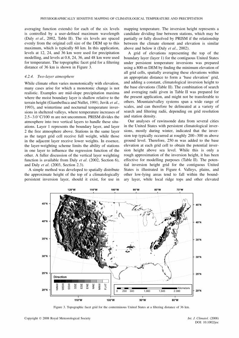
averaging function extends) for each of the six levelsis controlled by a user-defined maximum wavelength(Daly et al., 2002, Table II). The six levels are spacedevenly from the original cell size of the DEM up to thismaximum, which is typically 60 km. In this application,levels at 12, 24, and 36 km were used for precipitationmodelling, and levels at 0.8, 24, 36, and 48 km were usedfor temperature. The topographic facet grid for a filteringdistance of 36 km is shown in Figure 3.
4.2.4. Two-layer atmosphere
While climate often varies monotonically with elevation,many cases arise for which a monotonic change is notrealistic. Examples are mid-slope precipitation maximawhere the moist boundary layer is shallow relative to theterrain height (Giambelluca and Nullet, 1991; Juvik et al.,1993), and wintertime and nocturnal temperature inver-sions in sheltered valleys, where temperature increases of2.5–3.0 °C/100 m are not uncommon. PRISM divides theatmosphere into two vertical layers to handle these situ-ations. Layer 1 represents the boundary layer, and layer2 the free atmosphere above. Stations in the same layeras the target grid cell receive full weight, while thosein the adjacent layer receive lower weights. In essence,the layer-weighting scheme limits the ability of stationsin one layer to influence the regression function of theother. A fuller discussion of the vertical layer weightingfunction is available from Daly et al. (2002, Section 6),and Daly et al. (2003, Section 2.3).
A simple method was developed to spatially distributethe approximate height of the top of a climatologicallypersistent inversion layer, should it exist, for use in
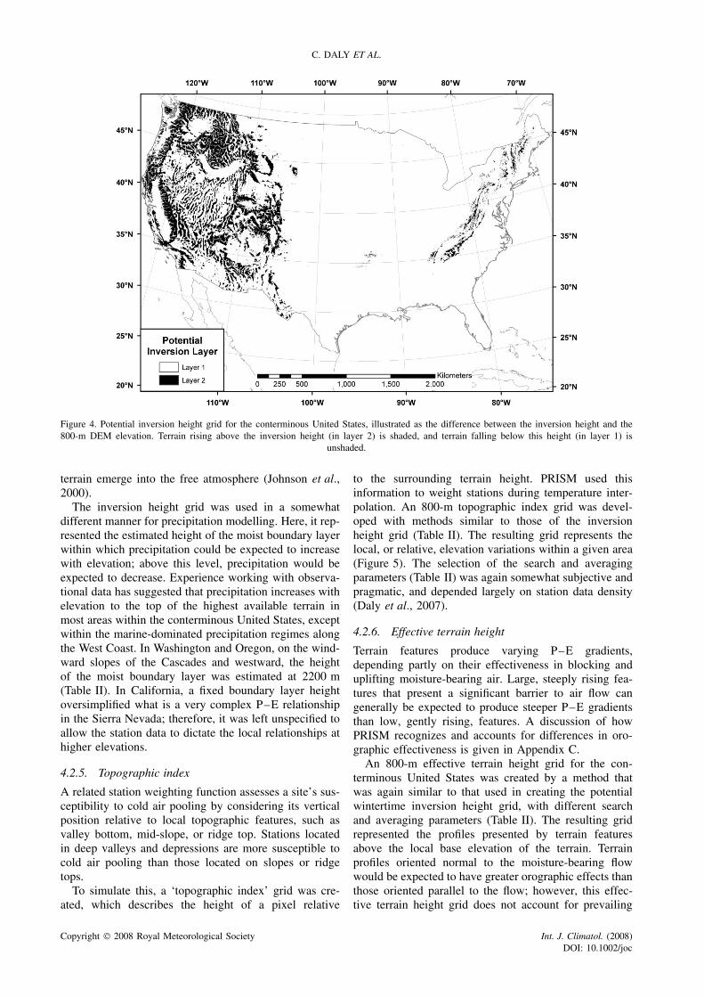
mapping temperature. The inversion height represents acandidate dividing line between stations, which may bepartially or fully dissolved by PRISM if the relationshipbetween the climate element and elevation is similarabove and below it (Daly et al., 2002).
A grid of elevations representing the top of theboundary layer (layer 1) for the contiguous United Statesunder persistent temperature inversions was preparedusing a 800-m DEM by finding the minimum elevation ofall grid cells, spatially averaging these elevations withinan appropriate distance to form a ‘base elevation’ grid,and adding a constant, climatological inversion height tothe base elevations (Table II). The combination of searchand averaging radii given in Table II was prepared forthe present application, and might not be transferable toothers. Mountain/valley systems span a wide range ofscales, and can therefore be delineated at a variety ofsearch and filtering radii, depending on grid resolutionand station density.
Our analyses of rawinsonde data from several citiesin the United States with persistent climatological inver-sions, mostly during winter, indicated that the inver-sion top typically occurred at roughly 200–300 m aboveground level. Therefore, 250 m was added to the baseelevation at each grid cell to obtain the potential inver-sion height above sea level. While this is only arough approximation of the inversion height, it has beeneffective for modelling purposes (Table II). The poten-tial inversion height grid for the contiguous UnitedStates is illustrated in Figure 4. Valleys, plains, andother low-lying areas tend to fall within the bound-ary layer, while local ridge tops and other elevated
Figure 3. Topographic facet grid for the conterminous United States at a filtering distance of 36 km.
Copyright 2008 Royal Meteorological Society Int. J. Climatol. (2008)DOI: 10.1002/joc
C. DALY ET AL.
Figure 4. Potential inversion height grid for the conterminous United States, illustrated as the difference between the inversion height and the800-m DEM elevation. Terrain rising above the inversion height (in layer 2) is shaded, and terrain falling below this height (in layer 1) is
unshaded.
terrain emerge into the free atmosphere (Johnson et al.,2000).
The inversion height grid was used in a somewhatdifferent manner for precipitation modelling. Here, it rep-resented the estimated height of the moist boundary layerwithin which precipitation could be expected to increasewith elevation; above this level, precipitation would beexpected to decrease. Experience working with observa-tional data has suggested that precipitation increases withelevation to the top of the highest available terrain inmost areas within the conterminous United States, exceptwithin the marine-dominated precipitation regimes alongthe West Coast. In Washington and Oregon, on the wind-ward slopes of the Cascades and westward, the heightof the moist boundary layer was estimated at 2200 m(Table II). In California, a fixed boundary layer heightoversimplified what is a very complex P–E relationshipin the Sierra Nevada; therefore, it was left unspecified toallow the station data to dictate the local relationships athigher elevations.
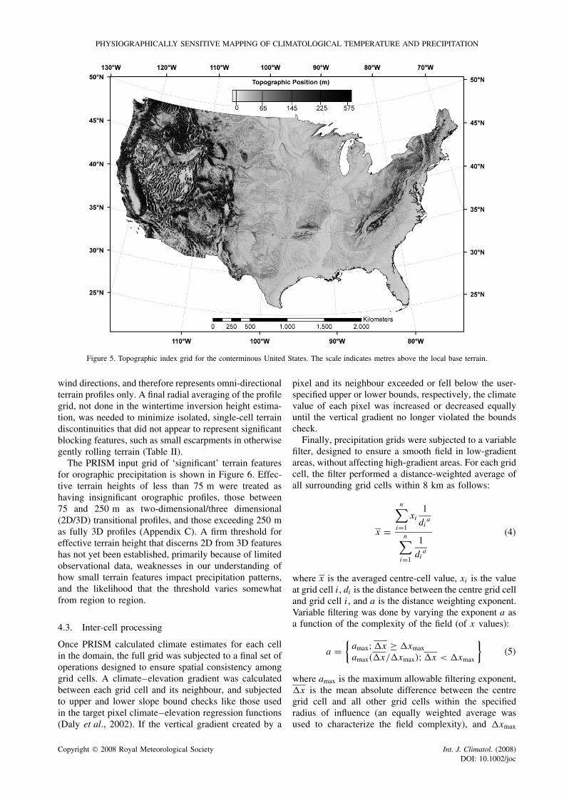
4.2.5. Topographic index
A related station weighting function assesses a site’s sus-ceptibility to cold air pooling by considering its verticalposition relative to local topographic features, such asvalley bottom, mid-slope, or ridge top. Stations locatedin deep valleys and depressions are more susceptible tocold air pooling than those located on slopes or ridgetops.
To simulate this, a ‘topographic index’ grid was cre-ated, which describes the height of a pixel relative
to the surrounding terrain height. PRISM used thisinformation to weight stations during temperature inter-polation. An 800-m topographic index grid was devel-oped with methods similar to those of the inversionheight grid (Table II). The resulting grid represents thelocal, or relative, elevation variations within a given area(Figure 5). The selection of the search and averagingparameters (Table II) was again somewhat subjective andpragmatic, and depended largely on station data density(Daly et al., 2007).
4.2.6. Effective terrain height
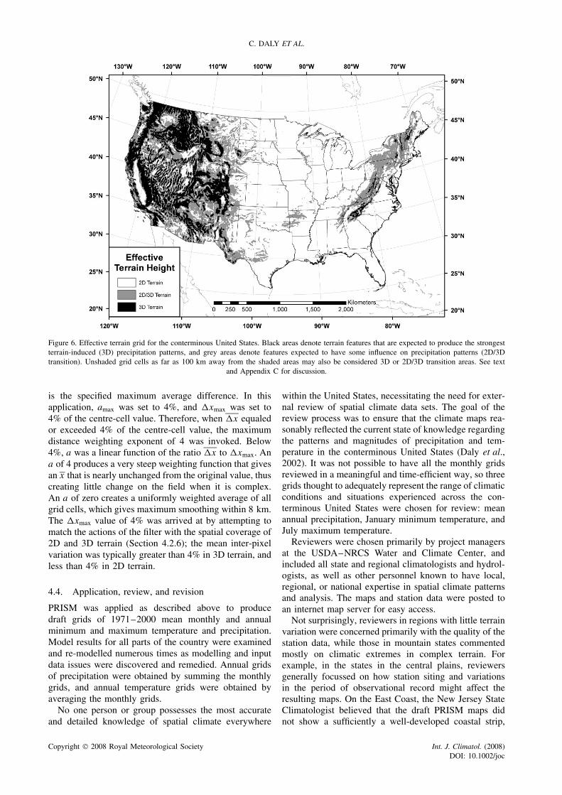
Terrain features produce varying P–E gradients,depending partly on their effectiveness in blocking anduplifting moisture-bearing air. Large, steeply rising fea-tures that present a significant barrier to air flow cangenerally be expected to produce steeper P–E gradientsthan low, gently rising, features. A discussion of howPRISM recognizes and accounts for differences in oro-graphic effectiveness is given in Appendix C.
An 800-m effective terrain height grid for the con-terminous United States was created by a method thatwas again similar to that used in creating the potentialwintertime inversion height grid, with different searchand averaging parameters (Table II). The resulting gridrepresented the profiles presented by terrain featuresabove the local base elevation of the terrain. Terrainprofiles oriented normal to the moisture-bearing flowwould be expected to have greater orographic effects thanthose oriented parallel to the flow; however, this effec-tive terrain height grid does not account for prevailing
Copyright 2008 Royal Meteorological Society Int. J. Climatol. (2008)DOI: 10.1002/joc
PHYSIOGRAPHICALLY SENSITIVE MAPPING OF CLIMATOLOGICAL TEMPERATURE AND PRECIPITATION
Figure 5. Topographic index grid for the conterminous United States. The scale indicates metres above the local base terrain.
wind directions, and therefore represents omni-directionalterrain profiles only. A final radial averaging of the profilegrid, not done in the wintertime inversion height estima-tion, was needed to minimize isolated, single-cell terraindiscontinuities that did not appear to represent significantblocking features, such as small escarpments in otherwisegently rolling terrain (Table II).
The PRISM input grid of ‘significant’ terrain featuresfor orographic precipitation is shown in Figure 6. Effec-tive terrain heights of less than 75 m were treated ashaving insignificant orographic profiles, those between75 and 250 m as two-dimensional/three dimensional(2D/3D) transitional profiles, and those exceeding 250 mas fully 3D profiles (Appendix C). A firm threshold foreffective terrain height that discerns 2D from 3D featureshas not yet been established, primarily because of limitedobservational data, weaknesses in our understanding ofhow small terrain features impact precipitation patterns,and the likelihood that the threshold varies somewhatfrom region to region.
4.3. Inter-cell processing
Once PRISM calculated climate estimates for each cellin the domain, the full grid was subjected to a final set ofoperations designed to ensure spatial consistency amonggrid cells. A climate–elevation gradient was calculatedbetween each grid cell and its neighbour, and subjectedto upper and lower slope bound checks like those usedin the target pixel climate–elevation regression functions(Daly et al., 2002). If the vertical gradient created by a
pixel and its neighbour exceeded or fell below the user-specified upper or lower bounds, respectively, the climatevalue of each pixel was increased or decreased equallyuntil the vertical gradient no longer violated the boundscheck.
Finally, precipitation grids were subjected to a variablefilter, designed to ensure a smooth field in low-gradientareas, without affecting high-gradient areas. For each gridcell, the filter performed a distance-weighted average ofall surrounding grid cells within 8 km as follows:
x =
n∑i=1
xi
1
dia
n∑i=1
1
dia
(4)
where x is the averaged centre-cell value, xi is the valueat grid cell i, di is the distance between the centre grid celland grid cell i, and a is the distance weighting exponent.Variable filtering was done by varying the exponent a asa function of the complexity of the field (of x values):
a ={
amax;�x ≥ �xmax
amax(�x/�xmax); �x < �xmax
}(5)
where amax is the maximum allowable filtering exponent,�x is the mean absolute difference between the centregrid cell and all other grid cells within the specifiedradius of influence (an equally weighted average wasused to characterize the field complexity), and �xmax
Copyright 2008 Royal Meteorological Society Int. J. Climatol. (2008)DOI: 10.1002/joc
C. DALY ET AL.
Figure 6. Effective terrain grid for the conterminous United States. Black areas denote terrain features that are expected to produce the strongestterrain-induced (3D) precipitation patterns, and grey areas denote features expected to have some influence on precipitation patterns (2D/3Dtransition). Unshaded grid cells as far as 100 km away from the shaded areas may also be considered 3D or 2D/3D transition areas. See text
and Appendix C for discussion.
is the specified maximum average difference. In thisapplication, amax was set to 4%, and �xmax was set to4% of the centre-cell value. Therefore, when �x equaledor exceeded 4% of the centre-cell value, the maximumdistance weighting exponent of 4 was invoked. Below4%, a was a linear function of the ratio �x to �xmax. Ana of 4 produces a very steep weighting function that givesan x that is nearly unchanged from the original value, thuscreating little change on the field when it is complex.An a of zero creates a uniformly weighted average of allgrid cells, which gives maximum smoothing within 8 km.The �xmax value of 4% was arrived at by attempting tomatch the actions of the filter with the spatial coverage of2D and 3D terrain (Section 4.2.6); the mean inter-pixelvariation was typically greater than 4% in 3D terrain, andless than 4% in 2D terrain.
4.4. Application, review, and revision
PRISM was applied as described above to producedraft grids of 1971–2000 mean monthly and annualminimum and maximum temperature and precipitation.Model results for all parts of the country were examinedand re-modelled numerous times as modelling and inputdata issues were discovered and remedied. Annual gridsof precipitation were obtained by summing the monthlygrids, and annual temperature grids were obtained byaveraging the monthly grids.
No one person or group possesses the most accurateand detailed knowledge of spatial climate everywhere
within the United States, necessitating the need for exter-nal review of spatial climate data sets. The goal of thereview process was to ensure that the climate maps rea-sonably reflected the current state of knowledge regardingthe patterns and magnitudes of precipitation and tem-perature in the conterminous United States (Daly et al.,2002). It was not possible to have all the monthly gridsreviewed in a meaningful and time-efficient way, so threegrids thought to adequately represent the range of climaticconditions and situations experienced across the con-terminous United States were chosen for review: meanannual precipitation, January minimum temperature, andJuly maximum temperature.
Reviewers were chosen primarily by project managersat the USDA–NRCS Water and Climate Center, andincluded all state and regional climatologists and hydrol-ogists, as well as other personnel known to have local,regional, or national expertise in spatial climate patternsand analysis. The maps and station data were posted toan internet map server for easy access.
Not surprisingly, reviewers in regions with little terrainvariation were concerned primarily with the quality of thestation data, while those in mountain states commentedmostly on climatic extremes in complex terrain. Forexample, in the states in the central plains, reviewersgenerally focussed on how station siting and variationsin the period of observational record might affect theresulting maps. On the East Coast, the New Jersey StateClimatologist believed that the draft PRISM maps didnot show a sufficiently a well-developed coastal strip,
Copyright 2008 Royal Meteorological Society Int. J. Climatol. (2008)DOI: 10.1002/joc
PHYSIOGRAPHICALLY SENSITIVE MAPPING OF CLIMATOLOGICAL TEMPERATURE AND PRECIPITATION
where temperatures were warmer in winter and coolerin summer than adjacent inland areas (D. Robinson,pers. comm.). PRISM’s coastal proximity weightingexponent was increased to resolve this issue. A U.S.Forest Service scientist doing field work came acrossseveral U.S. Geologic Survey precipitation gauges onremote mountaintops in Nevada, and was able to locateand provide data from them (D. Westfall, pers. comm.).A Nevada Division of Water Resources scientist wasable to provide precipitation data from a local networkwhich improved estimates on the eastern slope of theSierra Nevada (J. Huntington, pers. comm.). Overall, thereviews raised important issues, expanded the station datasets, and improved the final product.
‘Final’ grids were produced on the basis of the reviewsreceived. The word ‘final’ is given in quotes, becausethere have been, and likely will be, small changes made tothese grids as issues are discovered and corrected. Userscan download all the current monthly grids and access alog of changes at http://prism.oregonstate.edu.
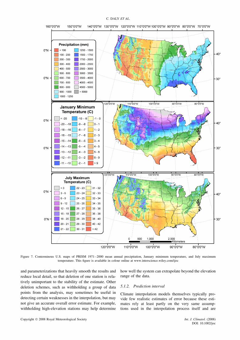
5. Results and performance evaluation
Maps of mean annual precipitation, January minimumtemperature, and July maximum temperature are shownin Figure 7. Average vertical gradients in precipitationand temperature are summarized by region in Table V. Avertical gradient was calculated for each pixel by findingthe average climate–elevation gradient between the pixeland the four surrounding pixels. The vertical gradientsamong pixels reported here, and in the PRISM diagnosticgrids shown in subsequent figures, usually do not matchthe weighted regression slopes calculated by PRISM.This is especially true if adjacent pixels are in differentphysiographic situations than the target pixel, e.g. a valleybottom pixel and adjacent hillslope pixels, because thePRISM regression slope reflects the relationship betweenclimate and elevation only for stations matching the targetcell’s physiographic characteristics.
While the maps in Figure 7 do not show much detailat this scale, some features are notable. Rain shadowsdownwind of the coastal, Olympic, Cascade, and SierraNevada ranges are visible, as are increases in precipita-tion over most elevated terrain, including the AppalachianMountains. Over orographically significant terrain fea-tures (denoted 3D terrain in Figure 6), precipitationincreased by about 70–75% of the estimated cell valueper kilometre elevation in the western and central UnitedStates, and about 50% in the eastern United States(Table V). The mean increase in precipitation over allterrain was much lower than for 3D terrain only, espe-cially in the centre and east, where much of the terrainis not orographically significant.
January minimum temperature exhibited very complexpatterns in the western United States, characterizedby numerous cold ‘ponds’ in valleys and depressions:temperatures were relatively mild along the ocean andGreat Lakes coastlines. The mean rate of change with
Table V. Vertical gradients in temperature and precipitation,summarized by effective terrain height (precipitation) and layer
(temperature).
Element Region
West Cent East
Mean annual precipitation3D terrain precipitation gradient (%/km) 75.45 71.02 50.71Overall precipitation gradient (%/km) 55.42 7.14 11.93
January minimum temperatureLayer 1 temperature gradient (°C/km) 2.33 −0.82 −2.83Layer 2 temperature gradient (°C/km) −2.45 −0.60 −1.65Overall temperature gradient (°C/km) 1.15 −0.79 −2.80
July maximum temperatureLayer 1 temperature gradient (°C/km) −5.74 −4.11 −3.78Layer 2 temperature gradient (°C/km) −7.50 −7.68 −7.42Overall temperature gradient (°C/km) −6.32 −4.21 −3.89
elevation was actually positive in layer 1 (white areasin Figure 6) in the western United States, reflectingthe dominance of temperature inversions in this region(Table V). The July maximum temperature exhibited astrong decrease with elevation across most of the country.Coastal areas were cooler than inland areas, especiallywhere the water temperature was significantly cooler thanthat of the land, such as along the West Coast. Regionallyaveraged vertical gradients were all negative, but positivegradients were common within the marine layer (layer 1)along most coastlines, including those in the central andeastern United States. Some of these features will bediscussed in greater detail in subsequent sections.
5.1. Statistical uncertainty analysisEstimating the true errors associated with spatial climatedata sets is difficult and subject to its own set of errors(Daly, 2006). This is because the true climate field isunknown, except at a relatively small number of observedpoints, and even these are subject to measurement andsiting uncertainties.
5.1.1. Cross-validation error
A performance statistic often reported in climate inter-polation studies is the cross-validation (C-V) error (Dalyet al., 1994; Willmott and Matsuura, 1995; Gyalistras,2003). C-V error is a measure of the difference betweenone or more station values and the model’s estimates forthose stations, when the stations have been removed fromthe data set. In the common practice of single-deletionjackknife C-V, the process of removal and estimation isperformed for each station one at a time, with the sta-tion returned to the data set after estimation. Once theprocess is complete, the overall error statistics, such asmean absolute error (MAE), bias, and others, are calcu-lated (e.g. Willmott et al., 1985; Legates and McCabe,1999). The obvious disadvantage to C-V error estima-tion is that no error information is provided for loca-tions where there are no stations. In addition, the single-deletion jackknife method favours interpolation models
Copyright 2008 Royal Meteorological Society Int. J. Climatol. (2008)DOI: 10.1002/joc
C. DALY ET AL.
Figure 7. Conterminous U.S. maps of PRISM 1971–2000 mean annual precipitation, January minimum temperature, and July maximumtemperature. This figure is available in colour online at www.interscience.wiley.com/ijoc
and parameterizations that heavily smooth the results andreduce local detail, so that deletion of one station is rela-tively unimportant to the stability of the estimate. Otherdeletion schemes, such as withholding a group of datapoints from the analysis, may sometimes be useful indetecting certain weaknesses in the interpolation, but maynot give an accurate overall error estimate. For example,withholding high-elevation stations may help determine
how well the system can extrapolate beyond the elevationrange of the data.
5.1.2. Prediction interval
Climate interpolation models themselves typically pro-vide few realistic estimates of error because these esti-mates rely at least partly on the very same assump-tions used in the interpolation process itself and are
Copyright 2008 Royal Meteorological Society Int. J. Climatol. (2008)DOI: 10.1002/joc
PHYSIOGRAPHICALLY SENSITIVE MAPPING OF CLIMATOLOGICAL TEMPERATURE AND PRECIPITATION
therefore neither independent nor reliable. These errorstatistics should only be used in a relative sense, with thesame model and station data set, and interpreted againstthe backdrop of model assumptions. However, modellederrors can be useful because they provide information atall grid cells, not just at station locations. The key toassessing the usefulness of modelled errors is to deter-mine how and to what extent they rely on model assump-tions, and assess how they compare with C-V errors.
Perhaps the most useful estimate of uncertainty pro-duced by PRISM is the regression prediction interval.Since PRISM uses weighted linear regression to estimateprecipitation or temperature as a function of elevation,standard methods for calculating prediction intervals forthe dependent variable (Y ) are used. Unlike a confidenceinterval, the prediction interval takes into account boththe variation in the possible location of the expected valueof Y for a given X (since the regression parameters mustbe estimated), and variation of individual values of Y
around the expected value (Neter et al., 1989). The for-mula used for calculating the variance of Y (temperatureor precipitation) for a new value of X = Xh (elevation)is:
s2{Yh(new)} = s2{Yh} + MSE = MSE
×
1 + 1
n∑i=1
wi
+ (Xh − X)2
n∑i=1
(wiXi − X)2
(6)
where s2{Yh} is the estimated variance of the expectedvalue of Yh at X = Xh, MSE is the regression meansquare error, X is the weighted mean elevation of theregression data set, and Xi and wi are the elevation andweight for station i, respectively (Neter et al., 1989). Theprediction interval at significance level α was created as:
Yh ± t1−α/2,df s{Yh} (7)
where t1−α/2,df is the 1 − (α/2) percentile value of thet distribution with df degrees of freedom for MSE. A(1 − α) of 0.70 (70%) was chosen for the predictioninterval because it approximated one standard deviation(where (1 − α) = 0.67) around the model prediction.Many model-based uncertainty estimates assume thatthe model is perfect, and therefore underestimate theuncertainty. For example, the kriging estimation varianceassumes the correctness of a simple semi-variogrammodel, and does not incorporate any uncertainty relatedto model goodness of fit (Daly, 2006). The PRISM 70%prediction interval, hereafter referred to as PI70, doesinclude this important source of variability.
As with any error estimate, PI70 has its strengthsand weaknesses. A major strength is that PI70 is largewhen there is a high degree of scatter about the localregression line, indicating a poor relationship between
climate and elevation and suggesting a poor predic-tion. This tends to occur at locations far from stations,in areas within transition zones between two or moreclimatic regimes (such as coastal temperature bound-aries or rain shadows), or at elevations in the verticaltransition between the boundary layer and free atmo-sphere during temperature inversions. PI70 also increasesthe farther the prediction is extrapolated away fromthe mean regression elevation. This is seen in highmountain areas that are well above the highest stationsin the vicinity, and therefore have uncertain predic-tions.
Unfortunately, the spatial patterns of PI70 are alsosensitive to the way in which PRISM is parameter-ized to weight stations. For example, the presenceof atmospheric-layer weighting produces PI70 patternsthat may be highly discontinuous in space, owing tomarkedly different stations being used above and belowthe inversion height. Without layer weighting, PI70 pat-terns become smoother and more generalized in space.In another example, the use of a minimum radius ofinfluence, rm (discussed in Section 4.2.1) affects PI70patterns. When rm is set to zero, PI70 at pixels con-taining station locations is reduced to near zero becausethe co-located stations dominate the weighted regression.However, when rm is set to 7–10 km (as was done forthis data set) and there are several nearby stations, PI70may not be reduced to zero because the weight of theco-located station does not dominate the regression func-tion. In essence, attempts to reduce bull’s eyes and otherisolated features in the interpolated field will often resultin increased PI70 values.
Finally, station weighting can often confound the effectthat df (degrees of freedom) has on PI70. Statistically, asdf decreases, PI70 increases. Therefore, in areas wherethere are few stations, the prediction interval shouldwiden, reflecting a more uncertain prediction. However,PRISM is parameterized to successively increase itsradius of influence until it retrieves a specified minimumnumber of stations for the regression function; thisminimum number is 15 stations for temperature and 40for precipitation. Therefore, df is always relatively high.However, station-weighting may favour only a handful ofthose stations with very large weights, leaving the otherswith vanishingly small weights, producing a regressionfunction with what is effectively very few stations (andusually limited scatter), but retaining the high df value.
A major weakness of both C-V error estimates andPI70, and which is somewhat counterintuitive, is thatthese error measures typically increase as the stationdata set becomes more comprehensive (Daly, 2006).For example, a low-elevation data set that does notresolve high mountain features may be easy to estimateand produce little scatter about the regression lines, butproduce very poor estimates in the mountains. In contrast,a station data set that spans a wide range of elevationsand samples more of the true variability in the climatefield would produce improved estimates, but likely bemore challenging for the model to simulate, resulting in
Copyright 2008 Royal Meteorological Society Int. J. Climatol. (2008)DOI: 10.1002/joc
C. DALY ET AL.
higher C-V errors and more scatter about the regressionlines.
5.1.3. Comparison of cross-validation errors andprediction intervals
C-V error and PI70 statistics for all months are summa-rized by region in Table VI, and illustrated spatially formean annual precipitation, January minimum tempera-ture, and July maximum temperature in Figures 8 and 9.C-V biases were very small for all the three climate ele-ments (not shown), less than 1 mm for precipitation and0.13 °C for temperature; this indicates that values werenot systematically over- or under-predicted. In general,regional mean C-V MAE and PI70 were surprisinglysimilar and were highest in the physiographically com-plex western United States (Table VI). For precipitation,C-V MAE and PI70 values in the western region werehighest in winter and lowest in summer, owing to thepredominance of winter-wet and summer-dry conditionsover much of the area. C-V MAE for precipitation wassomewhat higher in winter than PI70. Annually, both C-VMAE and PI70 were approximately 11% of the predictedgrid cell value (not shown). In the central and easternregions, PI70 was slightly higher than C-V MAE in mostmonths. Annually, both PI70’s and C-V MAEs wereabout 5% of the predicted grid cell value in the centralregion and about 4% in the east. The spatial distributionof percent C-V MAEs clearly shows a concentration ofrelatively large errors in the western mountains and inarid regions, with a few larger errors in the AppalachianMountains (Figure 8).
C-V MAEs and PI70’s for minimum temperature weregenerally higher than those for maximum temperature,likely a result of the increased complexity of the eleva-tion regression function. In the West, minimum temper-ature C-V MAEs and PI70’s exceeding 1 °C were notuncommon, while those for maximum temperature aver-aged about 0.7 °C (Table VI). Central and eastern errorswere similar, and ranged from 0.6 to 0.8 °C for minimumtemperature and about 0.5 °C for maximum temperature.Winter errors were slightly higher than summer errors.The spatial distribution of January minimum temperatureerrors was characterized by large errors in the westernUnited States, but there were a significant number oflarger errors in the central and eastern United States,as well (Figures 8(b) and 9(b)). This reflected the highspatial variability of minimum temperature, even in rela-tively gentle terrain. Relatively few stations showed largeC-V MAEs for July maximum temperature (Figures 8(c)and 9(c)). However, large errors were found in mountain-ous areas of the West, as well as in coastal areas adjacentto the Pacific and Atlantic Oceans and Great Lakes. Dur-ing summer, water temperatures are significantly lowerthan land temperatures in these areas, creating large tem-perature gradients across short horizontal distances (Daly,2006).
The similarity of the C-V MAE and PI70 error esti-mates seems to lend support to the idea that the PI70 isa reasonable substitute for C-V MAE between stations,
at least at the regional level. To determine how well thetwo error estimates agree at sub-regional scales, the west-ern United States was subdivided into regular grids withsuccessively smaller cell sizes (500, 400, 300, 200, and100 km) and the average C-V MAE and PI70 estimatesfor mean annual precipitation, January minimum tem-perature, and July maximum temperature compared ateach scale. Figure 10 shows the change in R2 of a lin-ear regression between the mean C-V MAE and PI70 asthe averaging scale changed. At small averaging scales,R2 was relatively low (0.2–0.5), indicating that therewas relatively poor agreement between C-V MAE andPI70 within small areas. However, as the size of thearea increased, R2 increased rapidly, reaching maximaof 0.75–0.85.
5.2. Comparison with other data sets
PRISM spatial climate data sets were compared to twoother spatial climate data sets of similar resolutionfor the conterminous United States: Daymet (Thorntonet al., 1997) and WorldClim (Hijmans et al., 2005). TheDaymet data set spans the conterminous United Statesat a resolution of 1 km, and has an averaging period of1980–1997. Approximately 6000 stations from the NWSCOOP and USDA NRCS SNOTEL networks were usedin the interpolation. Interpolation was performed with theDaymet model (Thornton et al., 1997). Daymet developslocal linear relationships between climate and elevationfor each grid cell on a DEM, using data from surroundingstations. Each station is weighted only by its distancefrom the target grid cell. This method takes into accountthe elevational variation of climate, but does not have theability to simulate non-monotonic relationships betweenclimate and elevation, such as temperature inversions, anddoes not explicitly account for terrain-induced climatictransitions or coastal effects (Daly, 2006). Daymet datasets can be accessed online at www.daymet.org.
The WorldClim data set is global in extent, and has aresolution of 30 arcsec. Station data used in the con-terminous United States were largely restricted to theUSHCN (Williams et al., 2004), which is the U.S. por-tion of the Global Historical Climate Network (GHCN).The USHCN consists of about 1200 COOP stationswith long-term records. Averaging period for the datavaried, but was typically 1950–2000. The WorldClimdata set was interpolated with ANUSPLIN (Hutchin-son, 1995), a method that fits thin-plate splines (usu-ally second- or third-order polynomials) through stationdata in three dimensions: latitude, longitude, and ele-vation. As with Daymet and PRISM, the relationshipbetween the climate variable and elevation can vary inspace, making the method suitable for large domains.Because a spline is by definition smoothly varying, thisapproach has difficulty simulating sharply varying cli-mate transitions, which are characteristic of tempera-ture inversions, rain shadows, and coastal effects (Daly,2006). WorldClim data sets can be accessed online atwww.worldclim.org.
Copyright 2008 Royal Meteorological Society Int. J. Climatol. (2008)DOI: 10.1002/joc
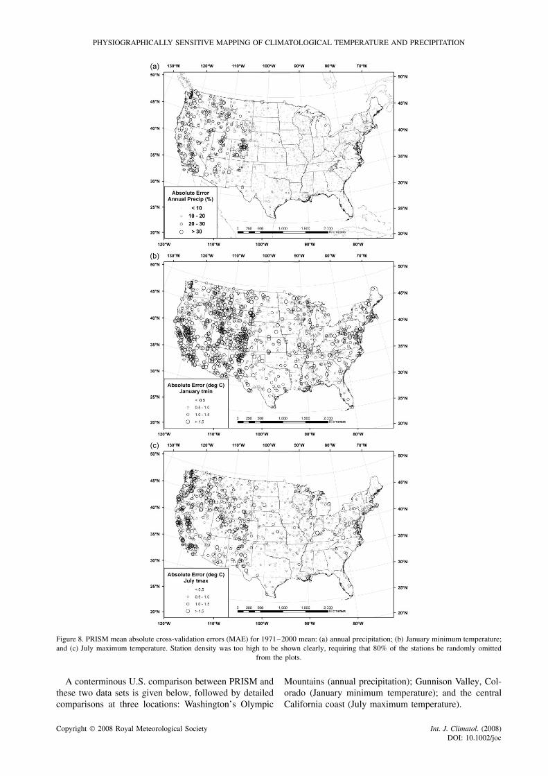
PHYSIOGRAPHICALLY SENSITIVE MAPPING OF CLIMATOLOGICAL TEMPERATURE AND PRECIPITATION
Figure 8. PRISM mean absolute cross-validation errors (MAE) for 1971–2000 mean: (a) annual precipitation; (b) January minimum temperature;and (c) July maximum temperature. Station density was too high to be shown clearly, requiring that 80% of the stations be randomly omitted
from the plots.
A conterminous U.S. comparison between PRISM andthese two data sets is given below, followed by detailedcomparisons at three locations: Washington’s Olympic
Mountains (annual precipitation); Gunnison Valley, Col-orado (January minimum temperature); and the centralCalifornia coast (July maximum temperature).
Copyright 2008 Royal Meteorological Society Int. J. Climatol. (2008)DOI: 10.1002/joc
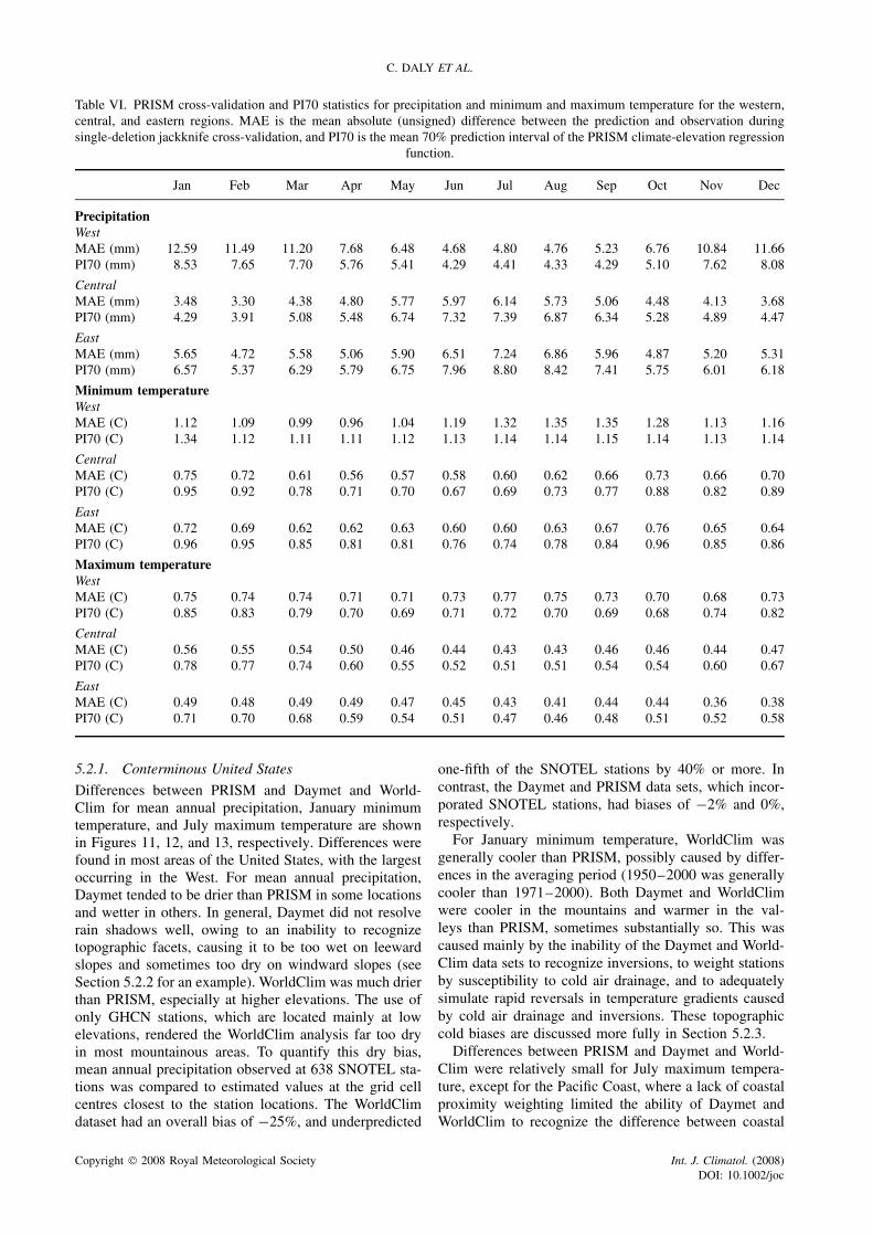
C. DALY ET AL.
Table VI. PRISM cross-validation and PI70 statistics for precipitation and minimum and maximum temperature for the western,central, and eastern regions. MAE is the mean absolute (unsigned) difference between the prediction and observation duringsingle-deletion jackknife cross-validation, and PI70 is the mean 70% prediction interval of the PRISM climate-elevation regression
function.
Jan Feb Mar Apr May Jun Jul Aug Sep Oct Nov Dec
PrecipitationWestMAE (mm) 12.59 11.49 11.20 7.68 6.48 4.68 4.80 4.76 5.23 6.76 10.84 11.66PI70 (mm) 8.53 7.65 7.70 5.76 5.41 4.29 4.41 4.33 4.29 5.10 7.62 8.08
CentralMAE (mm) 3.48 3.30 4.38 4.80 5.77 5.97 6.14 5.73 5.06 4.48 4.13 3.68PI70 (mm) 4.29 3.91 5.08 5.48 6.74 7.32 7.39 6.87 6.34 5.28 4.89 4.47
EastMAE (mm) 5.65 4.72 5.58 5.06 5.90 6.51 7.24 6.86 5.96 4.87 5.20 5.31PI70 (mm) 6.57 5.37 6.29 5.79 6.75 7.96 8.80 8.42 7.41 5.75 6.01 6.18
Minimum temperatureWestMAE (C) 1.12 1.09 0.99 0.96 1.04 1.19 1.32 1.35 1.35 1.28 1.13 1.16PI70 (C) 1.34 1.12 1.11 1.11 1.12 1.13 1.14 1.14 1.15 1.14 1.13 1.14
CentralMAE (C) 0.75 0.72 0.61 0.56 0.57 0.58 0.60 0.62 0.66 0.73 0.66 0.70PI70 (C) 0.95 0.92 0.78 0.71 0.70 0.67 0.69 0.73 0.77 0.88 0.82 0.89
EastMAE (C) 0.72 0.69 0.62 0.62 0.63 0.60 0.60 0.63 0.67 0.76 0.65 0.64PI70 (C) 0.96 0.95 0.85 0.81 0.81 0.76 0.74 0.78 0.84 0.96 0.85 0.86
Maximum temperatureWestMAE (C) 0.75 0.74 0.74 0.71 0.71 0.73 0.77 0.75 0.73 0.70 0.68 0.73PI70 (C) 0.85 0.83 0.79 0.70 0.69 0.71 0.72 0.70 0.69 0.68 0.74 0.82
CentralMAE (C) 0.56 0.55 0.54 0.50 0.46 0.44 0.43 0.43 0.46 0.46 0.44 0.47PI70 (C) 0.78 0.77 0.74 0.60 0.55 0.52 0.51 0.51 0.54 0.54 0.60 0.67
EastMAE (C) 0.49 0.48 0.49 0.49 0.47 0.45 0.43 0.41 0.44 0.44 0.36 0.38PI70 (C) 0.71 0.70 0.68 0.59 0.54 0.51 0.47 0.46 0.48 0.51 0.52 0.58
5.2.1. Conterminous United States
Differences between PRISM and Daymet and World-Clim for mean annual precipitation, January minimumtemperature, and July maximum temperature are shownin Figures 11, 12, and 13, respectively. Differences werefound in most areas of the United States, with the largestoccurring in the West. For mean annual precipitation,Daymet tended to be drier than PRISM in some locationsand wetter in others. In general, Daymet did not resolverain shadows well, owing to an inability to recognizetopographic facets, causing it to be too wet on leewardslopes and sometimes too dry on windward slopes (seeSection 5.2.2 for an example). WorldClim was much drierthan PRISM, especially at higher elevations. The use ofonly GHCN stations, which are located mainly at lowelevations, rendered the WorldClim analysis far too dryin most mountainous areas. To quantify this dry bias,mean annual precipitation observed at 638 SNOTEL sta-tions was compared to estimated values at the grid cellcentres closest to the station locations. The WorldClimdataset had an overall bias of −25%, and underpredicted
one-fifth of the SNOTEL stations by 40% or more. Incontrast, the Daymet and PRISM data sets, which incor-porated SNOTEL stations, had biases of −2% and 0%,respectively.
For January minimum temperature, WorldClim wasgenerally cooler than PRISM, possibly caused by differ-ences in the averaging period (1950–2000 was generallycooler than 1971–2000). Both Daymet and WorldClimwere cooler in the mountains and warmer in the val-leys than PRISM, sometimes substantially so. This wascaused mainly by the inability of the Daymet and World-Clim data sets to recognize inversions, to weight stationsby susceptibility to cold air drainage, and to adequatelysimulate rapid reversals in temperature gradients causedby cold air drainage and inversions. These topographiccold biases are discussed more fully in Section 5.2.3.
Differences between PRISM and Daymet and World-Clim were relatively small for July maximum tempera-ture, except for the Pacific Coast, where a lack of coastalproximity weighting limited the ability of Daymet andWorldClim to recognize the difference between coastal
Copyright 2008 Royal Meteorological Society Int. J. Climatol. (2008)DOI: 10.1002/joc
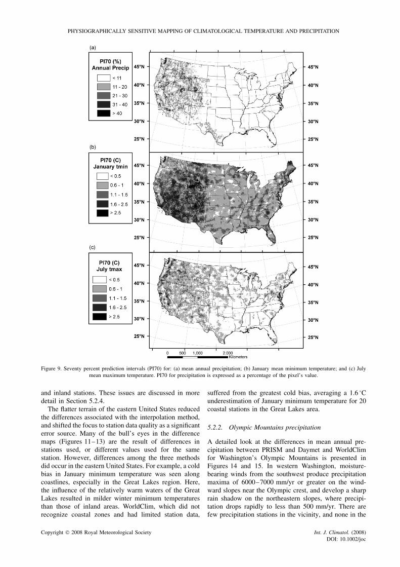
PHYSIOGRAPHICALLY SENSITIVE MAPPING OF CLIMATOLOGICAL TEMPERATURE AND PRECIPITATION
Figure 9. Seventy percent prediction intervals (PI70) for: (a) mean annual precipitation; (b) January mean minimum temperature; and (c) Julymean maximum temperature. PI70 for precipitation is expressed as a percentage of the pixel’s value.
and inland stations. These issues are discussed in moredetail in Section 5.2.4.
The flatter terrain of the eastern United States reducedthe differences associated with the interpolation method,and shifted the focus to station data quality as a significanterror source. Many of the bull’s eyes in the differencemaps (Figures 11–13) are the result of differences instations used, or different values used for the samestation. However, differences among the three methodsdid occur in the eastern United States. For example, a coldbias in January minimum temperature was seen alongcoastlines, especially in the Great Lakes region. Here,the influence of the relatively warm waters of the GreatLakes resulted in milder winter minimum temperaturesthan those of inland areas. WorldClim, which did notrecognize coastal zones and had limited station data,
suffered from the greatest cold bias, averaging a 1.6 °Cunderestimation of January minimum temperature for 20coastal stations in the Great Lakes area.
5.2.2. Olympic Mountains precipitation
A detailed look at the differences in mean annual pre-cipitation between PRISM and Daymet and WorldClimfor Washington’s Olympic Mountains is presented inFigures 14 and 15. In western Washington, moisture-bearing winds from the southwest produce precipitationmaxima of 6000–7000 mm/yr or greater on the wind-ward slopes near the Olympic crest, and develop a sharprain shadow on the northeastern slopes, where precipi-tation drops rapidly to less than 500 mm/yr. There arefew precipitation stations in the vicinity, and none in the
Copyright 2008 Royal Meteorological Society Int. J. Climatol. (2008)DOI: 10.1002/joc
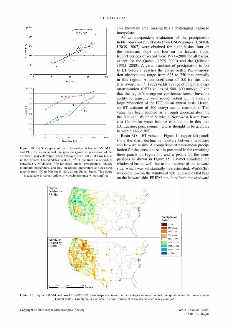
C. DALY ET AL.
Figure 10. (a) Scatterplot of the relationship between C-V MAEand PI70 for mean annual precipitation (given in percentage of theestimated grid cell value) when averaged over 300 × 300-km blocksin the western United States; and (b) R2 of the linear relationshipsbetween CV-MAE and PI70 for mean annual precipitation, Januaryminimum temperature, and July maximum temperature at block sizesranging from 100 to 500 km in the western United States. This figure
is available in colour online at www.interscience.wiley.com/ijoc
core mountain area, making this a challenging region tointerpolate.
As an independent evaluation of the precipitationfields, observed runoff data from USGS gauges (USDOI-USGS, 2007) were obtained for eight basins, four onthe windward slope and four on the leeward slope.Runoff periods of record were 1971–2000 for all basins,except for the Queets (1975–2000) and the Quilcene(1995–2000). A certain amount of precipitation is lostto ET before it reaches the gauge outlet. Pan evapora-tion observations range from 625 to 750 mm annuallyin this region. A pan coefficient of 0.8 for this area(Farnsworth et al., 1982) yields a range of potential evap-otranspiration (PET) values of 500–600 mm/yr. Giventhat the region’s evergreen coniferous forests have theability to transpire year round, actual ET is likely alarge proportion of the PET on an annual basis. Hence,an ET estimate of 500 mm/yr seems reasonable. Thisvalue has been adopted as a rough approximation bythe National Weather Service’s Northwest River Fore-cast Center for water balance calculations in this area(D. Laurine, pers. comm.), and is thought to be accurateto within about 30%.
Basin RO + ET values in Figure 14 (upper left panel)show the sharp decline in moisture between windwardand leeward basins. A comparison of basin-mean precip-itation for the three data sets is presented in the remainingthree panels of Figure 14, and a profile of the com-parisons is shown in Figure 15. Daymet simulated thewindward basins well, but at the expense of the leewardside, which was substantially overestimated. WorldClimwas quite low on the windward side, and somewhat highon the leeward side. PRISM simulated both the windward
Figure 11. Daymet/PRISM and WorldClim/PRISM ratio maps (expressed as percentage) of mean annual precipitation for the conterminousUnited States. This figure is available in colour online at www.interscience.wiley.com/ijoc
Copyright 2008 Royal Meteorological Society Int. J. Climatol. (2008)DOI: 10.1002/joc
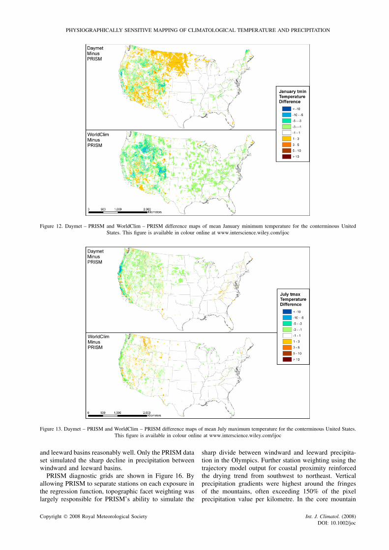
PHYSIOGRAPHICALLY SENSITIVE MAPPING OF CLIMATOLOGICAL TEMPERATURE AND PRECIPITATION
Figure 12. Daymet – PRISM and WorldClim – PRISM difference maps of mean January minimum temperature for the conterminous UnitedStates. This figure is available in colour online at www.interscience.wiley.com/ijoc
Figure 13. Daymet – PRISM and WorldClim – PRISM difference maps of mean July maximum temperature for the conterminous United States.This figure is available in colour online at www.interscience.wiley.com/ijoc
and leeward basins reasonably well. Only the PRISM dataset simulated the sharp decline in precipitation betweenwindward and leeward basins.
PRISM diagnostic grids are shown in Figure 16. Byallowing PRISM to separate stations on each exposure inthe regression function, topographic facet weighting waslargely responsible for PRISM’s ability to simulate the
sharp divide between windward and leeward precipita-tion in the Olympics. Further station weighting using thetrajectory model output for coastal proximity reinforcedthe drying trend from southwest to northeast. Verticalprecipitation gradients were highest around the fringesof the mountains, often exceeding 150% of the pixelprecipitation value per kilometre. In the core mountain
Copyright 2008 Royal Meteorological Society Int. J. Climatol. (2008)DOI: 10.1002/joc
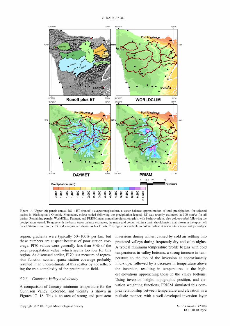
C. DALY ET AL.
Figure 14. Upper left panel: annual RO + ET (runoff + evapotranspiration), a water balance approximation of total precipitation, for selectedbasins in Washington’s Olympic Mountains, colour-coded following the precipitation legend. ET was roughly estimated at 500 mm/yr for allbasins. Remaining panels: WorldClim, Daymet, and PRISM mean annual precipitation grids, with basin overlays, also colour-coded following theprecipitation legend. To agree with the basin water balance estimates, the mean grid colour within a basin should match that shown in the upper leftpanel. Stations used in the PRISM analysis are shown as black dots. This figure is available in colour online at www.interscience.wiley.com/ijoc
region, gradients were typically 50–100% per km, butthese numbers are suspect because of poor station cov-erage. PI70 values were generally less than 30% of thepixel precipitation value, which seems too low for thisregion. As discussed earlier, PI70 is a measure of regres-sion function scatter; sparse station coverage probablyresulted in an underestimate of this scatter by not reflect-ing the true complexity of the precipitation field.
5.2.3. Gunnison Valley and vicinity
A comparison of January minimum temperature for theGunnison Valley, Colorado, and vicinity is shown inFigures 17–18. This is an area of strong and persistent
inversions during winter, caused by cold air settling intoprotected valleys during frequently dry and calm nights.A typical minimum temperature profile begins with coldtemperatures in valley bottoms, a strong increase in tem-perature to the top of the inversion at approximatelymid-slope, followed by a decrease in temperature abovethe inversion, resulting in temperatures at the high-est elevations approaching those in the valley bottoms.Using inversion height, topographic position, and ele-vation weighting functions, PRISM simulated this com-plex relationship between temperature and elevation in arealistic manner, with a well-developed inversion layer
Copyright 2008 Royal Meteorological Society Int. J. Climatol. (2008)DOI: 10.1002/joc
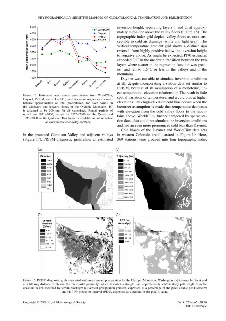
PHYSIOGRAPHICALLY SENSITIVE MAPPING OF CLIMATOLOGICAL TEMPERATURE AND PRECIPITATION
Figure 15. Estimated mean annual precipitation from WorldClim,Daymet, PRISM, and RO + ET (runoff + evapotranspiration), a waterbalance approximation of total precipitation, for river basins onthe windward and leeward slopes of the Olympic Mountains. ETis assumed to be 500 mm for all watersheds. Runoff periods ofrecord are 1971–2000, except for 1975–2000 on the Queets and1995–2000 on the Quilcene. This figure is available in colour online
at www.interscience.wiley.com/ijoc
in the protected Gunnison Valley and adjacent valleys(Figure 17). PRISM diagnostic grids show an estimated
inversion height, separating layers 1 and 2, at approxi-mately mid-slope above the valley floors (Figure 18). Thetopographic index grid depicts valley floors as most sus-ceptible to cold air drainage (white and light grey). Thevertical temperature gradient grid shows a distinct signreversal, from highly positive below the inversion heightto negative above. As might be expected, PI70 estimatesexceeded 3 °C in the uncertain transition between the twolayers where scatter in the regression function was great-est, and fell to 1.5 °C or less in the valleys and in themountains.
Daymet was not able to simulate inversion conditionsat all, despite incorporating a station data set similar toPRISM, because of its assumption of a monotonic, lin-ear temperature–elevation relationship. The result is littlespatial variation of temperature, and a cold bias at higherelevations. This high-elevation cold bias occurs when theincorrect assumption is made that temperature decreaseswith elevation from the cold valley floors to the moun-tains above. WorldClim, further hampered by sparse sta-tion data, also could not simulate the inversion conditionsand had an even more pronounced cold bias than Daymet.
Cold biases of the Daymet and WorldClim data setsin western Colorado are illustrated in Figure 19. Here,369 stations were grouped into four topographic index
Figure 16. PRISM diagnostic grids associated with mean annual precipitation for the Olympic Mountains, Washington: (a) topographic facet gridat a filtering distance of 36 km; (b) PW coastal proximity, which describes a straight line, approximately southwesterly path length from thecoastline in km, modified by terrain blockage; (c) vertical precipitation gradient, expressed as a percentage of the pixel’s value per kilometre;
and (d) 70% prediction interval (PI70), expressed as a percent of the pixel’s value.
Copyright 2008 Royal Meteorological Society Int. J. Climatol. (2008)DOI: 10.1002/joc
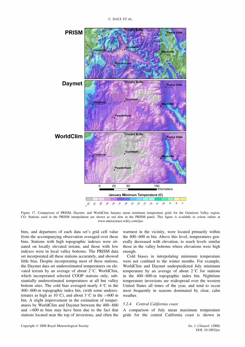
C. DALY ET AL.
Figure 17. Comparison of PRISM, Daymet, and WorldClim January mean minimum temperature grids for the Gunnison Valley region,CO. Stations used in the PRISM interpolation are shown as red dots in the PRISM panel. This figure is available in colour online at
www.interscience.wiley.com/ijoc
bins, and departures of each data set’s grid cell valuefrom the accompanying observation averaged over thesebins. Stations with high topographic indexes were sit-uated on locally elevated terrain, and those with lowindexes were in local valley bottoms. The PRISM dataset incorporated all these stations accurately, and showedlittle bias. Despite incorporating most of these stations,the Daymet data set underestimated temperatures on ele-vated terrain by an average of about 2 °C. WorldClim,which incorporated selected COOP stations only, sub-stantially underestimated temperatures at all but valleybottom sites. The cold bias averaged nearly 4 °C in the400–600-m topographic index bin, (with some underes-timates as high as 10 °C), and about 3 °C in the >600 mbin. A slight improvement in the estimation of temper-atures by WorldClim and Daymet between the 400–600and >600 m bins may have been due to the fact thatstations located near the top of inversions, and often the
warmest in the vicinity, were located primarily withinthe 400–600 m bin. Above this level, temperatures gen-erally decreased with elevation, to reach levels similarthose in the valley bottoms where elevations were highenough.
Cold biases in interpolating minimum temperaturewere not confined to the winter months. For example,WorldClim and Daymet underpredicted July minimumtemperature by an average of about 2 °C for stationsin the 400–600-m topographic index bin. Nighttimetemperature inversions are widespread over the westernUnited States all times of the year, and tend to occurmost frequently in seasons dominated by clear, calmweather.
5.2.4. Central California coast
A comparison of July mean maximum temperaturegrids for the central California coast is shown in
Copyright 2008 Royal Meteorological Society Int. J. Climatol. (2008)DOI: 10.1002/joc
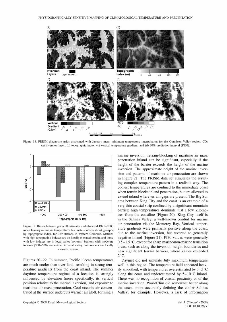
PHYSIOGRAPHICALLY SENSITIVE MAPPING OF CLIMATOLOGICAL TEMPERATURE AND PRECIPITATION
Figure 18. PRISM diagnostic grids associated with January mean minimum temperature interpolation for the Gunnison Valley region, CO:(a) inversion layer; (b) topographic index; (c) vertical temperature gradient; and (d) 70% prediction interval (PI70).
Figure 19. Biases between grid-cell estimates and observed 1971–2000mean January minimum temperatures (estimate – observation), groupedby topographic index, for 369 stations in western Colorado. Stationswith high topographic indexes are on locally elevated terrain, and thosewith low indexes are in local valley bottoms. Stations with moderateindexes (300–500) are neither in local valley bottoms nor on locally
elevated terrain.
Figures 20–22. In summer, Pacific Ocean temperaturesare much cooler than over land, resulting in strong tem-perature gradients from the coast inland. The summerdaytime temperature regime of a location is stronglyinfluenced by elevation (more specifically, its verticalposition relative to the marine inversion) and exposure tomaritime air mass penetration. Cool oceanic air concen-trated at the surface undercuts warmer air aloft, forming a
marine inversion. Terrain-blocking of maritime air masspenetration inland can be significant, especially if theheight of the barrier exceeds the height of the marineinversion. The approximate height of the marine inver-sion and patterns of maritime air penetration are shownin Figure 21. The PRISM data set simulates the result-ing complex temperature pattern in a realistic way. Thecoolest temperatures are confined to the immediate coastwhen terrain blocks inland penetration, but are allowed toextend inland where terrain gaps are present. The Big Surarea between King City and the coast is an example of avery thin coastal strip confined by a significant mountainbarrier; high temperatures dominate just a few kilome-tres from the coastline (Figure 20). King City itself isin the Salinas Valley, a well-known conduit for marineair penetration via the Monterey Bay. Vertical temper-ature gradients were primarily positive along the coast,due to the marine inversion, but reverted to generallynegative inland (Figure 21). PI70 values were generally0.5–1.5 °C, except for sharp marine/non-marine transitionareas, such as along the inversion height boundaries andnear significant terrain barriers, where values exceeded2 °C.
Daymet did not simulate July maximum temperaturewell in this region. The temperature field appeared heav-ily smoothed, with temperatures overestimated by 3–5 °Calong the coast and underestimated by 5–10 °C inland.There was no recognition of coastal proximity or of themarine inversion. WorldClim did somewhat better alongthe coast, more accurately defining the cooler SalinasValley, for example. However, a lack of information
Copyright 2008 Royal Meteorological Society Int. J. Climatol. (2008)DOI: 10.1002/joc
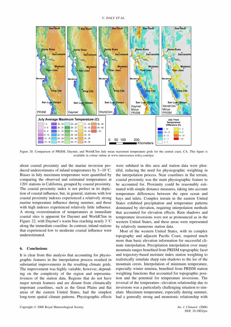
C. DALY ET AL.
Figure 20. Comparison of PRISM, Daymet, and WorldClim July mean maximum temperature grids for the central coast, CA. This figure isavailable in colour online at www.interscience.wiley.com/ijoc
about coastal proximity and the marine inversion pro-duced underestimates of inland temperatures by 3–10 °C.Biases in July maximum temperature were quantified bycomparing the observed and estimated temperatures at1201 stations in California, grouped by coastal proximity.The coastal proximity index is not perfect in its depic-tion of coastal influence, but, in general, stations with lowcoastal proximity indexes experienced a relatively strongmarine temperature influence during summer, and thosewith high indexes experienced relatively little influence.A strong overestimation of temperatures at immediatecoastal sites is apparent for Daymet and WorldClim inFigure 22, with Daymet’s warm bias reaching nearly 3 °Calong the immediate coastline. In contrast, inland stationsthat experienced low to moderate coastal influence wereunderestimated.
6. Conclusions
It is clear from this analysis that accounting for physio-graphic features in the interpolation process resulted insubstantial improvements in the resulting climate grids.The improvement was highly variable, however, depend-ing on the complexity of the region and representa-tiveness of the station data. Regions that do not havemajor terrain features and are distant from climaticallyimportant coastlines, such as the Great Plains and flatareas of the eastern United States, had the simplestlong-term spatial climate patterns. Physiographic effects
were subdued in this area and station data were plen-tiful, reducing the need for physiographic weighting inthe interpolation process. Near coastlines in flat terrain,coastal proximity was the main physiographic feature tobe accounted for. Proximity could be reasonably esti-mated with simple distance measures, taking into accounttemperature differences between the open ocean andbays and inlets. Complex terrain in the eastern UnitedStates exhibited precipitation and temperature patternsdominated by elevation, requiring interpolation methodsthat accounted for elevation effects. Rain shadows andtemperature inversions were not as pronounced as in thewestern United States, and these areas were representedby relatively numerous station data.
Most of the western United States, with its complextopography and adjacent Pacific Coast, required muchmore than basic elevation information for successful cli-mate interpolation. Precipitation interpolation over manymountain ranges benefited from PRISM topographic facetand trajectory-based moisture index station weighting torealistically simulate sharp rain shadows to the lee of themountain crests. Interpolation of minimum temperature,especially winter minima, benefited from PRISM stationweighting functions that accounted for topographic posi-tion and the potential for temperature inversions. Thereversal of the temperature–elevation relationship due toinversions was a particularly challenging situation to sim-ulate. Maximum temperature, especially during summer,had a generally strong and monotonic relationship with
Copyright 2008 Royal Meteorological Society Int. J. Climatol. (2008)DOI: 10.1002/joc
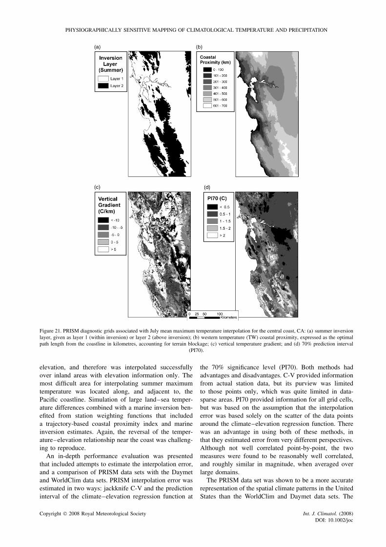
PHYSIOGRAPHICALLY SENSITIVE MAPPING OF CLIMATOLOGICAL TEMPERATURE AND PRECIPITATION
Figure 21. PRISM diagnostic grids associated with July mean maximum temperature interpolation for the central coast, CA: (a) summer inversionlayer, given as layer 1 (within inversion) or layer 2 (above inversion); (b) western temperature (TW) coastal proximity, expressed as the optimalpath length from the coastline in kilometres, accounting for terrain blockage; (c) vertical temperature gradient; and (d) 70% prediction interval
(PI70).
elevation, and therefore was interpolated successfullyover inland areas with elevation information only. Themost difficult area for interpolating summer maximumtemperature was located along, and adjacent to, thePacific coastline. Simulation of large land–sea temper-ature differences combined with a marine inversion ben-efited from station weighting functions that includeda trajectory-based coastal proximity index and marineinversion estimates. Again, the reversal of the temper-ature–elevation relationship near the coast was challeng-ing to reproduce.
An in-depth performance evaluation was presentedthat included attempts to estimate the interpolation error,and a comparison of PRISM data sets with the Daymetand WorldClim data sets. PRISM interpolation error wasestimated in two ways: jackknife C-V and the predictioninterval of the climate–elevation regression function at
the 70% significance level (PI70). Both methods hadadvantages and disadvantages. C-V provided informationfrom actual station data, but its purview was limitedto those points only, which was quite limited in data-sparse areas. PI70 provided information for all grid cells,but was based on the assumption that the interpolationerror was based solely on the scatter of the data pointsaround the climate–elevation regression function. Therewas an advantage in using both of these methods, inthat they estimated error from very different perspectives.Although not well correlated point-by-point, the twomeasures were found to be reasonably well correlated,and roughly similar in magnitude, when averaged overlarge domains.
The PRISM data set was shown to be a more accuraterepresentation of the spatial climate patterns in the UnitedStates than the WorldClim and Daymet data sets. The
Copyright 2008 Royal Meteorological Society Int. J. Climatol. (2008)DOI: 10.1002/joc
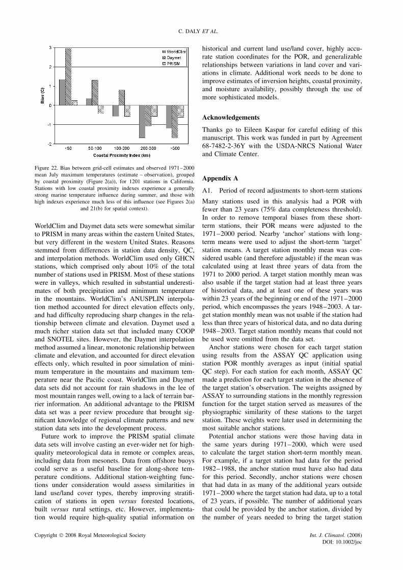
C. DALY ET AL.
Figure 22. Bias between grid-cell estimates and observed 1971–2000mean July maximum temperatures (estimate – observation), groupedby coastal proximity (Figure 2(a)), for 1201 stations in California.Stations with low coastal proximity indexes experience a generallystrong marine temperature influence during summer, and those withhigh indexes experience much less of this influence (see Figures 2(a)
and 21(b) for spatial context).
WorldClim and Daymet data sets were somewhat similarto PRISM in many areas within the eastern United States,but very different in the western United States. Reasonsstemmed from differences in station data density, QC,and interpolation methods. WorldClim used only GHCNstations, which comprised only about 10% of the totalnumber of stations used in PRISM. Most of these stationswere in valleys, which resulted in substantial underesti-mates of both precipitation and minimum temperaturein the mountains. WorldClim’s ANUSPLIN interpola-tion method accounted for direct elevation effects only,and had difficulty reproducing sharp changes in the rela-tionship between climate and elevation. Daymet used amuch richer station data set that included many COOPand SNOTEL sites. However, the Daymet interpolationmethod assumed a linear, monotonic relationship betweenclimate and elevation, and accounted for direct elevationeffects only, which resulted in poor simulation of mini-mum temperature in the mountains and maximum tem-perature near the Pacific coast. WorldClim and Daymetdata sets did not account for rain shadows in the lee ofmost mountain ranges well, owing to a lack of terrain bar-rier information. An additional advantage to the PRISMdata set was a peer review procedure that brought sig-nificant knowledge of regional climate patterns and newstation data sets into the development process.
Future work to improve the PRISM spatial climatedata sets will involve casting an ever-wider net for high-quality meteorological data in remote or complex areas,including data from mesonets. Data from offshore buoyscould serve as a useful baseline for along-shore tem-perature conditions. Additional station-weighting func-tions under consideration would assess similarities inland use/land cover types, thereby improving stratifi-cation of stations in open versus forested locations,built versus rural settings, etc. However, implementa-tion would require high-quality spatial information on
historical and current land use/land cover, highly accu-rate station coordinates for the POR, and generalizablerelationships between variations in land cover and vari-ations in climate. Additional work needs to be done toimprove estimates of inversion heights, coastal proximity,and moisture availability, possibly through the use ofmore sophisticated models.
Acknowledgements
Thanks go to Eileen Kaspar for careful editing of thismanuscript. This work was funded in part by Agreement68-7482-2-36Y with the USDA-NRCS National Waterand Climate Center.
Appendix A
A1. Period of record adjustments to short-term stations
Many stations used in this analysis had a POR withfewer than 23 years (75% data completeness threshold).In order to remove temporal biases from these short-term stations, their POR means were adjusted to the1971–2000 period. Nearby ‘anchor’ stations with long-term means were used to adjust the short-term ‘target’station means. A target station monthly mean was con-sidered usable (and therefore adjustable) if the mean wascalculated using at least three years of data from the1971 to 2000 period. A target station monthly mean wasalso usable if the target station had at least three yearsof historical data, and at least one of these years waswithin 23 years of the beginning or end of the 1971–2000period, which encompasses the years 1948–2003. A tar-get station monthly mean was not usable if the station hadless than three years of historical data, and no data during1948–2003. Target station monthly means that could notbe used were omitted from the data set.
Anchor stations were chosen for each target stationusing results from the ASSAY QC application usingstation POR monthly averages as input (initial spatialQC step). For each station for each month, ASSAY QCmade a prediction for each target station in the absence ofthe target station’s observation. The weights assigned byASSAY to surrounding stations in the monthly regressionfunction for the target station served as measures of thephysiographic similarity of these stations to the targetstation. These weights were later used in determining themost suitable anchor stations.
Potential anchor stations were those having data inthe same years during 1971–2000, which were usedto calculate the target station short-term monthly mean.For example, if a target station had data for the period1982–1988, the anchor station must have also had datafor this period. Secondly, anchor stations were chosenthat had data in as many of the additional years outside1971–2000 where the target station had data, up to a totalof 23 years, if possible. The number of additional yearsthat could be provided by the anchor station, divided bythe number of years needed to bring the target station
Copyright 2008 Royal Meteorological Society Int. J. Climatol. (2008)DOI: 10.1002/joc
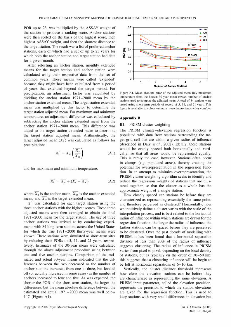
PHYSIOGRAPHICALLY SENSITIVE MAPPING OF CLIMATOLOGICAL TEMPERATURE AND PRECIPITATION
POR up to 23, was multiplied by the ASSAY weight ofthe station to produce a ranking score. Anchor stationswere then sorted on the basis of the highest score, thenhighest ASSAY weight, and then the shortest distance tothe target station. The result was a list of preferred anchorstations, each of which had a set of up to 23 years forwhich both the anchor station and target station had datafor a given month.
After selecting an anchor station, monthly extendedmeans for the target station and anchor station werecalculated using their respective data from the set ofcommon years. These means were called ‘extended’because they might have been calculated from a periodof years that extended beyond the target period. Forprecipitation, an adjustment factor was calculated bydividing the anchor station 1971–2000 mean by theanchor station extended mean. The target station extendedmean was multiplied by this factor to determine thetarget station adjusted mean. For maximum and minimumtemperature, an adjustment difference was calculated bysubtracting the anchor station extended mean from theanchor station 1971–2000 mean. This difference wasadded to the target station extended mean to determinethe target station adjusted mean. Arithmetically, thetarget adjusted mean (Xt
′) was calculated as follows for
precipitation:
Xt′ = Xte
(Xa
Xae
)(A1)
and for maximum and minimum temperature:
Xt′ = Xte + (Xa − Xae) (A2)
where Xa is the anchor mean, Xae is the anchor extendedmean, and Xte is the target extended mean.
Xt′
was calculated for each target station using thethree anchor stations with the highest scores. These threeadjusted means were then averaged to obtain the final1971–2000 mean for the target station. The use of threeanchor stations was arrived at by conducting experi-ments with 84 long-term stations across the United Statesfor which the true 1971–2000 thirty-year means wereknown. These stations were simulated as short-term sitesby reducing their PORs to 5, 11, and 21 years, respec-tively. Estimates of the 30-year mean were calculatedthrough the above adjustment procedure using betweenone and five anchor stations. Comparison of the esti-mated and actual 30-year means indicated that the dif-ferences between the two decreased as the number ofanchor stations increased from one to three, but leveledoff (or actually increased in some cases) as the number ofanchors increased to four and five. As was expected, theshorter the POR of the short-term station, the larger thedifferences, but the mean absolute difference between theestimated and actual 1971–2000 mean was well below1 °C (Figure A1).
Figure A1. Mean absolute error of the adjusted mean July maximumtemperature from the known 30-year mean versus number of anchorstations used to compute the adjusted mean. A total of 84 stations weretested using short-term periods of record of 5, 11, and 21 years. Thisfigure is available in colour online at www.interscience.wiley.com/ijoc
Appendix B
B1. PRISM cluster weighting
The PRISM climate–elevation regression function ispopulated with data from stations surrounding the tar-get grid cell that are within a given radius of influence(described in Daly et al., 2002). Ideally, these stationswould be evenly spaced both horizontally and verti-cally, so that all areas would be represented equally.This is rarely the case, however. Stations often occurin clumps (e.g. populated areas), thereby creating thepotential for overrepresentation in the regression func-tion. In an attempt to minimize overrepresentation, thePRISM cluster-weighting algorithm seeks to identify andreduce the regression weights of stations that are clus-tered together, so that the cluster as a whole has theapproximate weight of a single station.
How closely spaced can stations be before they arecharacterized as representing essentially the same point,and therefore perceived as clustered? Horizontally, howwe intuitively define a cluster varies with the scale of theinterpolation process, and is best related to the horizontalradius of influence within which stations are drawn for theregression function; the larger the radius of influence, thefarther stations can be spaced before they are perceivedto be clustered. Over the past decade of modelling withPRISM, it has been found that a horizontal separationdistance of less than 20% of the radius of influencesuggests clustering. The radius of influence in PRISMvaries from pixel to pixel, depending on the local densityof stations, but is typically on the order of 30–50 km;this suggests that a clustering influence will be begin tobe felt at horizontal separations of 6–10 km.
Vertically, the cluster distance threshold representshow close the elevation stations can be before theyare characterized as representing the same elevation. APRISM input parameter, called the elevation precision,represents the precision to which the station elevationsare given for the regression function. This is used tokeep stations with very small differences in elevation but
Copyright 2008 Royal Meteorological Society Int. J. Climatol. (2008)DOI: 10.1002/joc
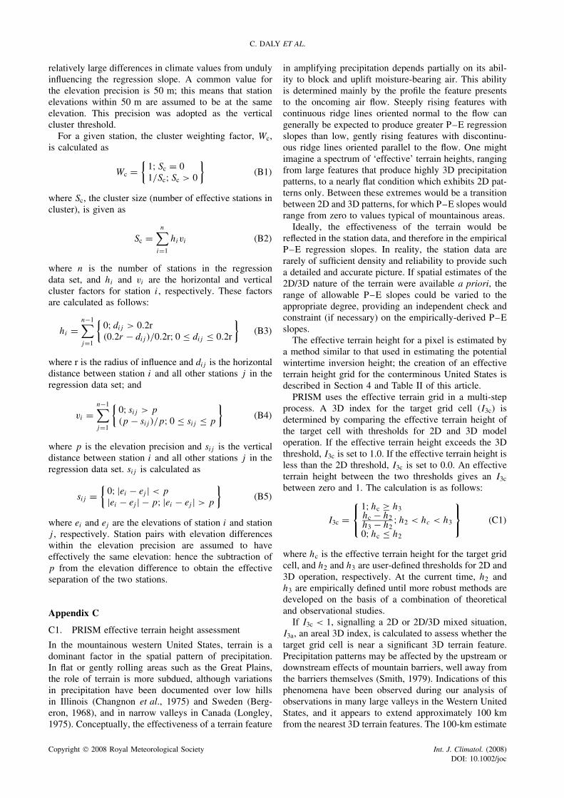
C. DALY ET AL.
relatively large differences in climate values from undulyinfluencing the regression slope. A common value forthe elevation precision is 50 m; this means that stationelevations within 50 m are assumed to be at the sameelevation. This precision was adopted as the verticalcluster threshold.
For a given station, the cluster weighting factor, Wc,is calculated as
Wc ={
1; Sc = 01/Sc; Sc > 0
}(B1)
where Sc, the cluster size (number of effective stations incluster), is given as
Sc =n∑
i=1
hivi (B2)
where n is the number of stations in the regressiondata set, and hi and vi are the horizontal and verticalcluster factors for station i, respectively. These factorsare calculated as follows:
hi =n−1∑j=1
{0; dij > 0.2r(0.2r − dij )/0.2r; 0 ≤ dij ≤ 0.2r
}(B3)
where r is the radius of influence and dij is the horizontaldistance between station i and all other stations j in theregression data set; and
vi =n−1∑j=1
{0; sij > p
(p − sij )/p; 0 ≤ sij ≤ p
}(B4)
where p is the elevation precision and sij is the verticaldistance between station i and all other stations j in theregression data set. sij is calculated as
sij ={
0; |ei − ej | < p
|ei − ej | − p; |ei − ej | > p
}(B5)
where ei and ej are the elevations of station i and stationj , respectively. Station pairs with elevation differenceswithin the elevation precision are assumed to haveeffectively the same elevation: hence the subtraction ofp from the elevation difference to obtain the effectiveseparation of the two stations.
Appendix C
C1. PRISM effective terrain height assessment
In the mountainous western United States, terrain is adominant factor in the spatial pattern of precipitation.In flat or gently rolling areas such as the Great Plains,the role of terrain is more subdued, although variationsin precipitation have been documented over low hillsin Illinois (Changnon et al., 1975) and Sweden (Berg-eron, 1968), and in narrow valleys in Canada (Longley,1975). Conceptually, the effectiveness of a terrain feature
in amplifying precipitation depends partially on its abil-ity to block and uplift moisture-bearing air. This abilityis determined mainly by the profile the feature presentsto the oncoming air flow. Steeply rising features withcontinuous ridge lines oriented normal to the flow cangenerally be expected to produce greater P–E regressionslopes than low, gently rising features with discontinu-ous ridge lines oriented parallel to the flow. One mightimagine a spectrum of ‘effective’ terrain heights, rangingfrom large features that produce highly 3D precipitationpatterns, to a nearly flat condition which exhibits 2D pat-terns only. Between these extremes would be a transitionbetween 2D and 3D patterns, for which P–E slopes wouldrange from zero to values typical of mountainous areas.
Ideally, the effectiveness of the terrain would bereflected in the station data, and therefore in the empiricalP–E regression slopes. In reality, the station data arerarely of sufficient density and reliability to provide sucha detailed and accurate picture. If spatial estimates of the2D/3D nature of the terrain were available a priori, therange of allowable P–E slopes could be varied to theappropriate degree, providing an independent check andconstraint (if necessary) on the empirically-derived P–Eslopes.
The effective terrain height for a pixel is estimated bya method similar to that used in estimating the potentialwintertime inversion height; the creation of an effectiveterrain height grid for the conterminous United States isdescribed in Section 4 and Table II of this article.
PRISM uses the effective terrain grid in a multi-stepprocess. A 3D index for the target grid cell (I3c) isdetermined by comparing the effective terrain height ofthe target cell with thresholds for 2D and 3D modeloperation. If the effective terrain height exceeds the 3Dthreshold, I3c is set to 1.0. If the effective terrain height isless than the 2D threshold, I3c is set to 0.0. An effectiveterrain height between the two thresholds gives an I3c
between zero and 1. The calculation is as follows:
I3c =
1;hc ≥ h3hc − h2h3 − h2
;h2 < hc < h3
0;hc ≤ h2
(C1)
where hc is the effective terrain height for the target gridcell, and h2 and h3 are user-defined thresholds for 2D and3D operation, respectively. At the current time, h2 andh3 are empirically defined until more robust methods aredeveloped on the basis of a combination of theoreticaland observational studies.
If I3c < 1, signalling a 2D or 2D/3D mixed situation,I3a, an areal 3D index, is calculated to assess whether thetarget grid cell is near a significant 3D terrain feature.Precipitation patterns may be affected by the upstream ordownstream effects of mountain barriers, well away fromthe barriers themselves (Smith, 1979). Indications of thisphenomena have been observed during our analysis ofobservations in many large valleys in the Western UnitedStates, and it appears to extend approximately 100 kmfrom the nearest 3D terrain features. The 100-km estimate
Copyright 2008 Royal Meteorological Society Int. J. Climatol. (2008)DOI: 10.1002/joc
PHYSIOGRAPHICALLY SENSITIVE MAPPING OF CLIMATOLOGICAL TEMPERATURE AND PRECIPITATION
is preliminary, and may be updated as more informationis gathered.
I3a is calculated similar to I3c:
I3a =
1; ha ≥ h3ha − h2h3 − h2
;h2 < ha < h3
0; ha ≤ h2
(C2)
where ha is a distance-weighted effective terrain height,calculated as
ha =
n∑i=1
wihi
n(C3)
where hi is the effective terrain height for grid cell i andn is the number of grid cells within 100 km of the targetgrid cell. The weight w for a nearby grid cell i is
wi = 1
di
(C4)
where di is the horizontal distance between the centresof the target grid cell and nearby grid cell i.
The final 3D index, I3d, is expressed as
I3d = max[I3c, I3a] (C5)
A scalar from 0 to 1, I3d represents the degree ofimportance terrain should play in the estimation of pre-cipitation. When I3d = 1, the PRISM regression functionoperates in its normal fashion. As I3d approaches zero,the influence of terrain is gradually diminished and valuesof terrain-related parameters – the minimum, maximum,and default regression slopes (β1m, β1x, and β1d); and theelevation, facet and layer weighting exponents (b, c, andy) – are linearly reduced to zero as a function of I3d (seeDaly et al., 2002, for definitions of PRISM parameters).When I3d is zero, the slope of the precipitation/elevationregression function is forced to zero and stations areweighted by distance, clustering, and coastal proximity(if enabled) only, resulting in a 2D interpolation.
References
Atkinson DE, Gajewski K. 2002. High-resolution estimation ofsummer surface air temperature in the Canadian Arctic Archipelago.Journal of Climate 15: 3601–3614.
Barnes SL. 1964. A technique for maximizing details in numericalweather map analysis. Journal of Applied Meteorology 3: 396–409.
Barry RG. 1992. Mountain Weather and Climate. Routledge: London.Barry RG, Chorley RJ. 1987. Atmosphere, Weather and Climate, 5th
edn. Routledge: London.Bergeron T. 1968. Studies of the Oreigenic Effect on the Areal fine
Structure of Rainfall Distribution . Meteorological Institute, UppsalaUniversity, Report No. 6.
Bolstad PV, Swift L, Collins F, Regniere J. 1998. Measured andpredicted air temperatures at basin to regional scales in the southernAppalachian Mountains. Agricultural and Forest Meteorology 91:161–176.
Bootsma A. 1976. Estimating minimum temperature and climatologicalfreeze risk in hilly terrain. Agricultural Meteorology 16: 425–443.
Brosofske KD, Chen J, Naiman RJ, Franklin JF. 1997. Harvestingeffects on microclimatic gradients from small streams to uplandsin western Washington. Ecological Applications 7: 1188–1200.
Changnon SA Jr, Jones DMA, Huff FA. 1975. Precipitation increasesin the low hills of southern Illinois. Part 2. Field investigation ofanomaly. Monthly Weather Review 103: 830–836.
Clements CB, Whiteman CD, Horel JD. 2003. Cold-air-pool structureand evolution in a mountain basin: Peter Sinks, Utah. Journal ofApplied Meteorology 42: 752–768.
Daley R. 1991. Atmospheric Data Analysis. Cambridge UniversityPress: Cambridge; 457.
Daly C. 2006. Guidelines for assessing the suitability of spatial climatedata sets. International Journal of Climatology 26: 707–721.
Daly C, Neilson RP, Phillips DL. 1994. A statistical-topographicmodel for mapping climatological precipitation over mountainousterrain. Journal of Applied Meteorology 33: 140–158.
Daly C, Helmer EH, Quinones M. 2003. Mapping the climate of PuertoRico, Vieques, and Culebra. International Journal of Climatology 23:1359–1381.
Daly C, Smith J, McKane R. 2007. High-resolution spatial modelingof daily weather elements for a catchment in the Oregon CascadeMountains, USA. Journal of Applied Meteorology and Climatology46: 1565–1586.
Daly C, Gibson WP, Taylor GH, Johnson GL, Pasteris P. 2002. Aknowledge-based approach to the statistical mapping of climate.Climate Research 22: 99–113.
Daly C, Taylor GH, Gibson WP, Parzybok TW, Johnson GL, Pas-teris P. 2001. High-quality spatial climate data sets for the UnitedStates and beyond. Transactions of the American Society of Agricul-tural Engineers 43: 1957–1962.
Daly C, Redmond K, Gibson W, Doggett M, Smith J, Taylor G,Pasteris P, Johnson G. 2005. Opportunities for improvementsin the quality control of climate observations. 15th AMSConference on Applied Climatology, American Meteorologi-cal Society: Savannah, GA, June 20–23, 2005. Paper J3.9.http://ams.confex.com/ams/pdfpapers/94199.pdf.
Daly C, Kittel TGF, McNab A, Gibson WP, Royle JA, Nychka D,Parzybok T, Rosenbloom N, Taylor G. 2000. Development of a103-year high-resolution climate data set for the conterminousUnited States. Proceedings of the 12th AMS Conference on AppliedClimatology. American Meteorological Society: Asheville, NC, May8–11, 249–252.
Davey CA, Pielke RA Sr. 2005. Microclimate exposures of surface-based weather stations–implications for the assessment of long-termtemperature trends. Bulletin of the American Meteorological Society86: 497–504.
Dong J, Chen J, Brosofske KD, Naiman RJ. 1998. Modelling airtemperature gradients across managed small streams in westernWashington. Journal of Environmental Management 53: 309–321.
Farnsworth R, Thompson ES, Peck EL. 1982. Evaporation Atlas forthe Contiguous 48 United States . NOAA Technical Report #33.
Funk C, Michaelsen J. 2004. A simplified diagnostic model oforographic rainfall for enhancing satellite-based rainfall estimates indata-poor regions. Journal of Applied Meteorology and Climatology43: 1366–1378.
Geiger R. 1964. The Climate Near the Ground. Harvard UniversityPress: Cambridge, MA; 611.
Giambelluca TW, Nullet D. 1991. Influence of the trade-wind inversionon the climate of a leeward mountain slope in Hawaii. ClimateResearch 1: 207–216.
Gibson WP, Daly C, Taylor GH. 1997. Derivation of facet gridsfor use with the PRISM model. Proceedings of the 10thAMS Conference on Applied Climatology. American Meteoro-logical Society: Reno, NV, Oct. 20–23, 208–209. Online athttp://prism.oregonstate.edu/pub/prism/docs/appclim97-facets-gibson.html.
Gibson WP, Daly C, Kittel T, Nychka D, Johns C, Rosenbloom N,McNab A, Taylor G. 2002. Development of a 103-year high-resolution climate data set for the conterminous United States.Proceedings of the 13th AMS Conference on Applied Climatology.American Meteorological Society: Portland, OR, May 13–16,181–183.
Gustavsson T, Karlsson M, Bogren J, Lindqvist S. 1998. Developmentof temperature patterns during clear nights. Journal of AppliedMeteorology 37: 559–571.
Gyalistras D. 2003. Development and validation of a high-resolutionmonthly gridded temperature and precipitation data set forSwitzerland (1951–2000). Climate Research 25: 55–83.
Hannaway DB, Daly C, Cao W, Luo W, Wei Y, Zhang W, Xu A,Lu C, Shi X, Li X. 2005. Forage species suitability mappingfor China using topographic, climatic and soils spatial data andquantitative plant tolerances. Scientia Agricultura Sinica 4: 660–667.
Copyright 2008 Royal Meteorological Society Int. J. Climatol. (2008)DOI: 10.1002/joc

C. DALY ET AL.
Haugen RK, Brown J. 1980. Coastal-inland distributions of summer airtemperature and precipitation in northern Alaska. Arctic and AlpineResearch 12: 403–412.
Hijmans RJ, Cameron SE, Parra JL, Jones PG, Jarvis A. 2005. Veryhigh resolution interpolated climate surfaces for global land areas.International Journal of Climatology 25: 1965–1978.
Hocevar A, Martsolf JD. 1971. Temperature distribution underradiation frost conditions in a central Pennsylvania valley.Agricultural Meteorology 8: 371–383.
Hutchinson MF. 1995. Interpolating mean rainfall using thinplate smoothing splines. International Journal of GeographicalInformation Science 9: 385–403.
Johnson GL, Daly C, Hanson CL, Lu YY, Taylor GH. 2000. Spatialvariability and interpolation of stochastic weather simulation modelparameters. Journal of Applied Meteorology 39: 778–796.
Juvik JO, Nullet D, Banko P, Hughes K. 1993. Forest climatology nearthe tree line in Hawai’i. Agricultural and Forest Meteorology 66:159–172.
Legates DR, McCabe GJ. 1999. Evaluating the use of “goodness of fit”measures in hydrologic and hydroclimatic model validation. WaterResources Research 35: 233–241.
Lindkvist L, Gustavsson T, Bogren J. 2000. A frost assessment methodfor mountainous areas. Agricultural and Forest Meteorology 102:51–67.
Longley RW. 1975. Precipitation in valleys. Weather 30: 294–300.Lookingbill T, Urban D. 2003. Spatial estimation of air temperature
differences for landscape-scale studies in montane environments.Agricultural and Forest Meteorology 114: 141–151.
Mahmood R, Foster SA, Logan D. 2006. The GeoProfile metadata,exposure of instruments, and measurement bias in climatic recordrevisited. International Journal of Climatology 26: 1091–1124.
McCutchan MH, Fox DG. 1986. Effect of elevation and aspect onwind, temperature and humidity. Journal of Climate and AppliedMeteorology 25: 1996–2013.
Mendonca BG, Iwaoka WT. 1969. The trade wind inversion at theslopes of Mauna Loa, Hawaii. Journal of Applied Meteorology 8:213–219.
Milewska EJ, Hopkinson RF, Niitsoo A. 2005. Evaluation of geo-referenced grids of 1961–1990 Canadian temperature andprecipitation normals. Atmosphere-Ocean 43: 49–75.
Neter J, Wasserman W, Kutner MH. 1989. Applied Linear RegressionModels, 2nd edn. Richard D. Irwin, Inc: Boston, MA.
NOAA-NCDC. 2003. Data Documentation for data set 3220,Summary of the Month Cooperative. National Climatic DataCenter, National Oceanic and Atmospheric Administration.http://www1.ncdc.noaa.gov/pub/data/documentlibrary/tddoc/td3220.pdf.
Oke TR. 1978. Boundary Layer Climates. Routledge: New York.Schwarb M, Daly C, Frei C, Schar C. 2001a. Mean seasonal
precipitation throughout the European Alps, 1971–1990 . HydrologicAtlas of Switzerland, National Hydrologic Service, Bern,Switzerland, hard copy.
Schwarb M, Daly C, Frei C, Schar C. 2001b. Mean Annual Precipita-tion Throughout the European Alps, 1971–1990 . Hydrologic Atlas ofSwitzerland, National Hydrologic Service, Bern, Switzerland, hardcopy.
Sharples JJ, Hutchinson MF, Jellet DR. 2005. On the horizontal scaleof elevation dependence of Australian monthly precipitation. Journalof Applied Meteorology 44: 1850–1865.
Simpson JJ, Hufford GL, Daly C, Berg JS, Fleming MD. 2005.Comparing maps of mean monthly surface temperature andprecipitation for Alaska and adjacent areas of Canada produced bytwo different methods. Arctic 58: 137–161.
Smith RB. 1979. The influence of mountains on the atmosphere.Advances in Geophysics 21: 87–230.
Thornton PE, Running SW, White MA. 1997. Generating surfaces ofdaily meteorological variables over large regions of complex terrain.Journal of Hydrology 190: 214–251.
USDA-NRCS. 1998. PRISM Climate Mapping Project–Precipitation .Mean monthly and annual precipitation digital files for thecontinental U.S. USDA-NRCS National Cartography and GeospatialCenter, Ft. Worth TX. December, CD-ROM and online.http://www.ncgc.nrcs.usda.gov/products/datasets/climate/.
USDOI-USGS. 2007. Calendar year Streamflow Statistics for Washing-ton . Water Resources of Washington, US Geologic Survey, Boulder,CO, available online at http://water.usgs.gov/wa/nwis/annual.
Williams CN, Vose RS, Easterling DR, Menne MJ. 2004. United StatesHistorical Climatology Network Daily Temperature, Precipitation,and Snow Data . ORNL/CDIAC-118, NDP-070. Carbon DioxideInformation Analysis Center, Oak Ridge National Laboratory, OakRidge, Tennessee.
Willmott CJ, Matsuura K. 1995. Smart Interpolation of annuallyaveraged air temperature in the United States. Journal of AppliedMeteorology 34: 2577–2586.
Willmott CJ, Ackleson SG, Davis RE, Feddema JJ, Klink KM,Legates DR, O’Donnell L, Rowe CM. 1985. Statistics for theevaluation and comparison of models. Journal of Geophical Research90: 8995–9005.
WMO. 1989. Calculation of Monthly and Annual 30-year StandardNormals . Prepared by a meeting of experts, Washington, DC, USA,March 1989. World Meteorological Organization, WCDP 10, WMO-TD 341.
Copyright 2008 Royal Meteorological Society Int. J. Climatol. (2008)DOI: 10.1002/joc
Recommended