-
-
-
-
PHOTOPRODUCTION OF CHARMED BARYONS
by
Mark C. Gibney
B.A., University of California, San Diego, 1980
A thesis submitted to the
Faculty of the Graduate School of the
University of Colorado in partial fulfillment
of the requirements for the degree of
Doctor of Philosophy
Department of Physics
1989

-
-
-

-
-
-
-
-
-
This thesis for the Doctor of Philosophy degree by
Mark Gibney
has been approved for the
Department of Physics
by
John Cumalat
Date APR.1L ~S- i9P:-\ )

-
-
-
-
..
-
-
-
-
-
-
-
-
Gibney, Mark C., (Ph.D., Physics)
Photoproduction of Charmed Baryons
Thesis directed by Professor Uriel N auenberg
Measurements of the branching fractions of the four At decay
modes, A0 7r+, A07r+7r+7r-, pKO, and pK0 7r+7r- relative to the At ---t
pK-7r+ decay mode are presented. The experiment was performed at the
Tagged Photon Spectrometer in the Proton East area of the Fermi Na
tional Accelerator Laboratory. The Tagged Photon Detector is a two
magnet spectrometer with large angular acceptance, good mass reso-
lution, and good particle identification. The particle identification is
achieved using Cerenkov counters, muon detectors, and electromagnetic
and hadronic calorimeters. Particle tracking and vertex detection are
accomplished by using a system of drift chambers in conjunction with
a set of high resolution silicon microstrip detectors. The construction,
maintenance, and calibration of the Cerenkov counters was the main re- .
sponsibility of the Colorado group.
The relative branching fractions for the four decay modes are
determined to be;
B(i\r.) . ~ B(pKr.) = 0.17 ± 0.08 ± O.Oo
B(i\r.r.7r) 9 B(pK 7r) = 0.82 ± 0.-9 ± 0.27
IV
B(pKO) B(pK7r) =0.55±0.17±0.14
B(pK07r7r) B(pK7r) < 1.7@90%CL.
These measurements are compared with existing theoretical results for
the two-body decays (A7r, pK0). Quark model and SU(4) calculations of
these branching fractions agree with our measurements while a similiar
calculation using the Bag Model disagrees. The resul.ts of this experiment
provide the needed corroboration for branching fraction measurements
made in e+e- collider experiments.
-
-
-

-
-
To Rhonda
For Her Love and Patience
-
-
-
-
-

ACKNOWLEDGMENTS
I begin by thanking the E691 collaboration:
University of Colorado, Boulder;
L. Cremaldi, J. Elliot, U. Nauenberg
University of California, Santa Barbara;
A. Bean, J. Duboscq, P. Karchin, S. McHugh, R. Morrison,
G. Punkar, J. Raab, M. Witherell
Carleton University;
P. Estabrooks, J. Pinfold, J. Sidhu
Centro Brasileiro de Pesquisas Fisicas;
J. Anjos, A. Santoro, M. Souza
Fermilab;
J. Appel, L. Chen, P. Mantsch, T. Nash, M. Purohit, K. Sliwa,
M. Sokoloff, W. Spalding, M. Streetman
National Research Council of Canada;
M. Losty
Universidade de Sao Paulo;
C. Escobar
University of Toronto;
S. Bracker, G. Hartner, B. Kumar, G. Luste, J. Martin,
S. Menary, P. Ong, G. Stairs, A. Stundzia
-

-
-
-
-
-
-
-
-
-
-
Vll
The dedication of these people was the first strength of the experiment.
The leadership provided during the run by Penny Estabrooks, Jeff Spald
ing, Steve Bracker, and Rolly Morrison was indispensible, inspiring, and
unforgettable. The leadership provided by Mike \Vitherell during the
data analysis was a lesson in leadership.
I personally thank my advisor, Uriel Nauenberg, for his patience, his guid
ance, his physics insight, and his patience. His encouragement through
out, and especially during the last few months, was not only appreciated
but necessary.
I personally thank Lucien Cremaldi for his encouragement, his physics
insight, and for reading this thesis (twice). The care and industry with
which he worked was an example to me.
I thank Jim Elliot for helping me progress from a naive to a real under
standing of how an experiment is done.
I thank Mike Sokoloff, Milind Purohit, Kris Sliwa, Ravi Kumar, and
Alice Bean for many insightful conversations on many topics (including
physics).
I thank my coworkers (Scott, Johannes, Tom, CW, Steve, Rich, Ray,
Wes, Tim, Tosa, Greg, Harry, and Janice) for their support.
And I thank the Brazilians for their friendliness and kindness (which
seemed to rub off).

Finally, I would like to thank those for whom thanks is not enough.
I thank my mother for her love and support.
viii
I thank Rhonda, to whom this thesis is dedicated, for her love, her pa
tience, and her encouragement.
And I thank my Lord, Jesus Christ, who has demonstrated through me
that the hopeless have hope. Indeed, 'I can do everything through him
who gives me strength'.
This work was supported by the U. S. Department of Energy.
-
-

-
-
-
-
-
-
CONTENTS
CHAPTER
1. Introduction . . . . . . . . . . . . . 1.1. The Fundamental Interactions
1.2. Predictions for Charmed Baryon Decays
1.3. Charm Production and Detection
1.3.1. Production
1.3.2. Detection . . . . . . .
1.4. A Brief History of Experiment E691
2. The Proton and Photon Beams
2.1. The Proton Beam
2.2. The Photon Beam
2.3. The Tagging System
3. The Detector
3.1. The Target
3.2. The Silicon Microstrip Detector
3.3. The Drift Chamber System
3.4. The Magnets . . . .
3.5. The Cerenkov Counters
3.5.1. The Counter Design
3.5.2. Monitoring
3.5.3. Calibration
3.6. The SLIC and the Pair Plane
3. 7. The Hadrometer
3.8. The Muon Wall
4. The Data Aquisition System
4.1. The Physics Triggers
4.2. The Data Recording
5. The Reconstruction Program
5.1. PASSl . . . . . . ..
5.2. PASS2
5.2.1. The SLIC Reconstruction Program
5.2.2. The Cerenkov Reconstruction Program
5.2.3. The Vertexing Reconstruction
1
1
7
10
10
12
14
15 15 16
21
25 r -0
27
31
36
37 . 38
. 52
. 54
60 63
64 67
67 70
74
75 76
76
. 78
. 81

6. The Analysis
6.1. The Neutral Particle Cuts 6.2. The Substrips
6.3. The Analysis Files
6.4. Monte Carlo Studies
7. Results ....... .
7.1. The Normalizing Mode: At-+ pK-7r+
7.2. The At -+ A o1r+1r+1r- Signal
7.3. The At -+ A 011'+ Signal
7.4. The At -+pKO Signal .
7.5. The At -+pK01r+1r- Signal
8. Result Comparisons and Conclusions
A Neutral Particle Efficiencies Al. Introduction . . . . . . . . .
A2. A Closer Look at o•+ -+ 1r+D0 -+ 1r+ Ko1r+1r
A3. The K• Study
A4. Conclusions
x
84
84
89
93 -102 114
114
115
120
123
125
128
137 137
139 142
146
-

-TABLES
Table
1.1.1 Characteristics of Quarks and Leptons 2
- 3.2.1 Characteristics of the Silicon Microstrip Detectors 28
3.3.1 Characteristics of the Drift Chambers 32
3.4.1 Characteristics of the TPL Magnets 37
3.5.1 Characteristics of the Cerenkov Counters 39
3.5.2 Cerenkov Cell Gains for Cl and C2 59
6.1. la Standard track Cuts 87
~- b Neutral Particle Cuts 87
6.2.la Substrip Cuts: A 01T'+1T'+7T'- 90
b Substrip Cuts: pK07T'+1T'- 90
- c Substrip Cuts: pKO 91
d Substrip Cuts: A 01T'+ 91
6.4.1 Monte Carlo Vertex Cut Study 111
- 6.4.2 Neutral Particle Efficiency Corrections 113
7.2.1 Final Cuts: A 01T'+ ?r+ 1T'- 117
7.3.1 Final Cuts: A 01T'+ 120
7.4.1 Final Cuts: pKO 123
7.5.l Final Cuts: pK01T'+1T'- 126
8.1.1 Charmed Baryon Relative Branching Fractions 131
-8.1.2 ;(~¥J) Experiment vs. Theory 131
Al.1 Corrected and Uncorrected Relative Branching Fractions 138
A2.1 Neutral Particle Efficiency Correction Factors Using K 0 1T'7T' 141
-

xii
A2.2 Neutral Efficiency Corrections Derived from the K 07r7r Correction Factors for the Charm Decay Modes . . . . . . . . 141
A3.l Neutral Particle Efficiency Correction Factors Using K•s 143
A3.2 Neutral Efficiency Corrections Derived from the K• Correction Factors for the Charm Decay Modes . . . . . . . . . . . . 143
-
-
-
-
--
FIGURES
Figure - 1.2.1 Decay Diagrams of the At Baryon 8
1.3.1 Photon-Gluon Fusion 11
2.1.1 Fixed Target Beamlines 17
2.2.1 PEAST Beamline . 18
2.2.2 Fractional Electron Yield vs. Fractional Electron Energy 20
2.3.1 The Tagging System 22 - 3.0.1 The Tagged Photon Spectrometer 26
3.2.1 Cross-section of a Silicon Microstrip Plane 29
3.3.2 TO Distribution . 35
3.5.1 Predicted and Observed Momentum Spectrum of the Tracks 40
3.5.2 Threshold Behaviour of the Cerenkov Counters 41
3.5.3 Schematic of the Cerenkov Counters 42
- 3.5.4 Mirror Patterns of the Cerenkov Counters 43
3.5.5 The Mirror Testing Apparatus 45
3.5.6 Mirror Refiectivities 46
3.5.7 Schematic of the Winston Cones 47 -3.5.8 Single Photo-Electron Pea.ks 49
3.5.9 Cerenkov Light Optics 53
3.5.10 The Response of the Cerenkov Counters to Data Events 55 -3.5.11 Gain Curves 56
3.5.12 Measured Threshold Behavior of the Cerenkov Counters 61
3.6.1 Schematic of the SLIC 62 - 3.7.1 Schematic of the Hadrometer 65
-
4.1.2 Charm Enhancement vs. Transverse Energy
4.2.1 The Data Aquisition System
5.2.1 Charm Vertex Event
6.1.1 Neutral (A0 and K,,) Signals vs. Neutral Particle Cuts
xiv
71
73
83
86
6.2.1 Proton Cerenkov Probabilities for Monte Carlo and Data 94
6.3.1 The Two-Body Cut Parameters . . . . 98
6.3.2 The Two-Body Vertex Error Derivation 100
6.3.3 The A"[ --+ A 1r Decay: The Cosine of the Angle between the Bach-elor Pion and the At Direction in the At Center of Mass 101
6.4.1 The Behaviour of the D0 -+K-1r+ with Standard Vertex Cuts 106
6.4.2 The Behaviour of the D0 -+K-1r+ with Modified Two-Body Vertex Cuts (Excluding the Kaon) . . . . . . . . . . . . . . 107
6.4.3 The Behaviour of the D0 -+K-1r+ with Modified Two-Body Vertex Cuts (Excluding the Pion) . . . . . . . . . . . . . . . 108
6.4.4 Stability of the A 0 and K. Signals with respect to the Neutral Par-ticle Cuts . . . . . . . . . . 110
7.1.1 The At -+pK-1r+ Invariant Mass 116
7.2.1 SDZ Distribution Plots for the A1r1r1r Mode 118
7.2.2 The At--+ A01r+1r+1r- Invariant Mass 119
7.3.1 SDZ Distribution Plots for the A1r Mode 121
7.3.2 The At --+ A 07r+ Invariant Mass 122
7.4.1 The At --+ pKO Invariant Mass 124
7.5.1 The At--+ pK01r+1r- Invariant Mass 127
A2.1 The Behaviour of n•+ --+ 1r+D0 --+ 1r+ K 01r+1r- with respect to Beam Energy, Kaon Transverse and Total Momentum, and the Number of Tracks . . . . . . . . . . . . . . . . . . . 140
A3.1 The Behaviour of K•+ --+ K 01r+ with respect to Beam Energy, Kaon Transverse and Total Momentum, and the Number of Tracks 145
-
-

-
-
-
-
-
-
-
-
-
CHAPTER 1
INTRODUCTION
High Energy Physics is the study of the very small. The smaller
the object we wish to 'see', the smaller the wavelength(>.,.) with which we
need to illuminate the object. In particular, photons used to probe these
objects must have high energies, since the photon wavelength is inversely
proportional to its energy. At present energies, >.,. ,...., 10-2 fermi, which is
the domain of quarks and leptons.
1.1 The Fundamental Interactions
Quarks were introduced by Gell-1'1ann 111 in the mid-sixties as a mneu
monic device to account for the many 'elementary' particles which had been
discovered during the decades before. The experimentalists had turned up
hundreds of these particles, each uniquely specified by its mass, decay rate,
spin, etc. The quark model succeeded in explaining the abundance of these
states as well as a good many of their characteristics, suggesting that the par
ticles observed in nature were actually composite particles. In Gell-Mann's
model, the experimentally observed particles were considered to be bound
states composed of combinations of three elementary particles of spin 1/2;
the up, down, and strange quarks. All physically observed states could be
classified in this scheme as either a quark-antiquark combination ( qq : me
son) or a three quark combination ( qqq and qqq : baryon and anti-baryon).
The quark structure of the proton (uud) was directly confirmed a few years
later in lepton-proton interaction experiments. r21 Table 1.1.1 shows that char-

2
Table 1.1.1 Characteristics of the Quarks and Leptons
Quark Spi11 Baryon N umbe1 Lepton Number ChargE
d(down) 1/2 1/3 0 -1/3 e
u(up) 1/2 1/3 0 +2/3 e
s(strange) 1/2 1/3 0 -1/3 e
c(charm) 1/2 1/3 0 +2/3 e
b(bottom) 1/2 1/3 0 -1/3 e
t(topr 1/2 1/3 0 +2/3 e
* the top quark is not established experimentally as yet
Lepton Spi11 Baryon Number Lepton N umbe1 Charge
Ve 1/2 0 1 Oe
e( electron) 1/2 0 1 -1 e ..,
Vµ 1/2 0 1 Oe
µ(muon) 1/2 0 1 -1 e
Vr 1/2 0 1 Oe
r(tau) 1/2 0 1 -1 e
-

-
-
-
-
-
-
-
-
-
3
acteristics of the quarks (deduced from the observed composite particles) as
well as the characteristics of the leptons.
The existence of the 6 ++ baryon, a symmetric state of three up
quarks ( uuu ), indicated that the theory, as proposed, was incomplete. Three
fermions cannot exist together in a symmetric state since they would then
violate Pauli's exclusion principle. To solve this problem, a new quantum
number called color was proposed. 131 This new degree of freedom could as
sume the three eigenvalues, red (r), green (g), and blue (b ); however, only
'colorless' combinations of these eigenvalues could be used to represent phys
ical states since the color quantum number is not observed in nature. The
color wavefunction for the ~ ++ is thus totally anti-symmetric, with the form;
WA++ ex: (rgb - rbg + brg - grb + gbr - bgr) (1.1.1)
where combinations of three unique colors are defined to be colorless. The
inclusion of the color quantum number in the quark model, thus, satisfied
the fermi statistics of the 6 ++ state. The color wavefunction of the mesons
likewise took the form;
w meson ex: ( rr + bb + gg) (1.1.2)
to complete this picture.
Experimental support for color was provided when the rate;
R = 11( e+ e- --+ hadrons) ,...., 2
u(e+e---+ µµ) ( 1.1.3)
was measured for center of mass energies below the charm threshold. (2! \\Tith-
out the color hypothesis, this rate would be three times smaller or ,...., 2/3,

4
given u ex (charge)2, and the charge of the quarks (i.e. R = ((2/3)2 + (1/3)2
+ (1/3)2)/12 = 2/3 without color). Color took its rightful place in the full
theory when it was recognized as the charge of the strong force. 1' 1
With this quark theory, all 'ordinary' mesons and baryons (those
composed of u, d, ands quarks) could be accounted for. The charm quark
was introduced into this scheme prior to the discovery of any charmed par
ticles to account for the conspicuous absence of particle decays with s -+ d
quark transitions. In the 3 quark ( uds) model, decays of this type are ex
pected to have significant branching fractions. 151 They are, however, strongly
suppressed, as evidenced by the ratio; 121
T(Kl -+ µµ) - -9 T(Kl -+all) - (9.1±1.9) x 10 (1.1.4)
where K~ -+ µµ can be considered as an s -+ dµµ decay. Thus, the
strangeness changing neutral current of the three quark model (ex d-y0 (1 -
-rs)s + s-y0 (1 - -rs)d to first order) must be suppressed somehow. Glashow,
Ilioupous, and Miani 111 demonstrated that the addition of the charm quark
to the quark model forced the cancellation of the first order term of this
current (and suppressed it to second order). The inclusion of this new quark
thus led to a revised theory which conformed to the experimental facts much
more closely.
If we include the leptons and the top* and bottom quarks in our set
of elementary particles, we have the following set of particles;
* Although the t=top quark hasn't been seen directly, the prevalence of b- c transitions over b-s transitions 1~1 provides some evidence for its existence since the GIM mechanism with which the flavor changing neutral currents (b - s) are suppressed required that the. quarks have a doublet struc~ure.
-
-

-
-
-
-
-
-
-
-
-
-
-
(~,) (:,) (~)
(:e) ( ~) ( ~).
5
(1.1.5)
The doublet structure given these particles implies that flavor changing neu
tral transitions are suppressed, 111 as was first demonstrated by Glashow, Il
ioupous, and Miani.
The d', s', b' introduced above are given by the expression;
(1.1.6)
where V is the Kobayashi-Maskawa matrix, 121 which relates the experimen
tally derived weak eigenstates (s') to their strong counterparts (s). The fact
that s f. s' implies that the weak decay products of the charm particle may
not contain a strange quark. Expressed quantitatively, c -+ s' =s xcosBe +
d xsin Be with Be = 13°, and thus 5% ( """'tan2Be) of the time the charm decay
products will contain a down instead of a strange quark. In this estimate,
we've used the simpler model of Cabbibo which excludes the top and bottom
quarks. The Kobayashi-Maskawa model includes this third 'generation' of
particles as a generalization of the Cabbibo model.
The interactions between these particles are categorized as electro
weak, strong, and gravitational and are characterized by the strength of the
interaction and its effective range. To begin with, the gravitational force
is negligible for the small quark and lepton masses, even for these small
distances. The remaining two forces are described using gauge: theories;
6
theories that remain invariant under some specific local gauge transforma
tion. Quantum electrodynamics (QED), of which the electro-weak theory
is an extension, is the simplest example of a gauge theory and is invari
ant with respect to local changes in the phase of the QED wavefunctions.
To illustrate the importance of this simple phase invariance, one can show
that the classical electromagnetic field is a direct consequence of the local
phase invariance of Schraedinger's equation. l7J In the realm of high energy
physics, the electro-weak model provides the (very successful) description of
the combined weak and electromagnetic forces, and quantum chromodynam
ics describes the strong force. These two gauge theories together are referred
to as the Standard Model.
The bosons which mediate these interactions are, respectively, the
photon (electromagnetic force)' the w+' the w-' and the zo (weak force)
of the electro-weak theory, and the 8 gluons which mediate the strong force.
The character of each of these forces can be related to the character of the
boson that mediates it. The photon is massless and thus the electromagnetic
force has 'infinite' range; its influence is felt directly over the classical distance
scale. The slow decay rate and small effective range which experimentally
separates the weak force from the other forces, is related to the large (,...,
lOOGeV /c2 ) masses of the w+·-(Mw ), and the Z0 (Mz) bosons. The weak
coupling is a full four orders of magnitude smaller than the ele<itromagnetic
coupling (aw ,..., (Mli'!Ji> ). Finally the experimentally supported concepts
of asymptotic freedom and quark confinement, 1' 1 behaviour unique to the
strong force, are related to the fact that the gluons interact with each other.
The character of the strong force makes charm physics particularly
intriguing. Asymptotic freedom (quark confinement) implies that the effect
-
-

-
-
-
-
-
7
of the strong force decreases (increases) with decreasing (increasing) distance
and thus perturbation theory applies most reliably to bound states of small
size, < < 1 fermi. The large charm quark mass naturally leads to smaller
bound statesc9J to which one might hope to apply perturbation theory with
some confidence.
1.2 Predictions for Charmed Baryon Decays
The A"d is the lowest mass charm baryon, with predicted quantum
numbers I(J)P = 0(1/2)+ and quark content (cud). As it has the lowest mass
of all the charmed baryons, it must decay weakly since flavor changing decays
are weak. The simplest form for the three decay topologies available to this
particle are the two W-emission diagrams shown in figure 1.2.lA (spectator
decay) and 1.2.lC and the W-exchange diagram shown in figure 1.2.lB (the
sea quarks have been omitted).
In the spectator decay shown in figure 1.2. lA, the charm quark emits
aw+ which converts to a ud quark pair(= 11'+). The up and down quarks
from the A"d are spectators to the decay in the sense that they take no part in
the weak interaction. The decay mechanism utilized by the diagram in figure
1.2.lC is also W-emission, as in the spectator decay. The final states gen
erated with this diagram can be quite different than those attained through
the simple spectator decay, however. Finally, W-exchange is shown in figure
1.2.lB. In this process, the charm and down quarks in the A"d exchange a
\V+, and a qq pair (at least one) is pulled from the sea. The specific two body
decay modes available to each of these diagrams are discussed elsewhere. [ioJ
The theoretical discussion of these decays is slim and limited to the
two body decays. All of the predictions are based on the charm flavor chang
ing effective Hamiltonian, Hee, in the short distance approximation; r11
·121

w• / ,{ u
/ c • (A)
d d
u u
c • d u
(B)
u u
c •
' a .. , '( u
(C)
u u
d d
FIGURE 1.2.1. Decay Diagrams of the A"t Baryon. (A) Spectator Decay. (B) W-Exchange Decay. (C) W-Emission.
8

-
-
-
-
-
-
-
9
(1.2.1)
with:
(1.2.2)
Only the Cabbibo favored term is kept in this approximation. The f+, L
coefficients measure the hard gluon contributions to equation 1.2.1, where
f+=L=l if strong interactions are ignored. Typically, L = 1.96 and f+ =
.64. [13]
Korner, Kramer, and \Villrodt 1111 have used the above effective
Hamiltonian (equation 1.2.2) to make predictions of the two body decays
of the At. In the first method used, they exploit the flavor symmetry of
the 0 ~ operators ( eqn. 1.2.3) of the effective Hamiltonian to obtain a large
set of 'sum rules' relating 6C=6S=l decays to established 6C=O decays.
Estimates were then obtained for the decay rates of the 6C=l decays using
the known behaviour of the non-chann decays. Clearly, the large symmetry
breaking mass differences between the charmed and ordinary baryons limits
the accuracy of this technique. They then use quark model wavefunctions
(described elsewhere) 1141 to calculate these decay rates. In this calculation,
the quark wavefunctions are inserted into a decay amplitude similiar to that
obtained using current algebra plus soft pion techniques.
10
The derivation of the amplitude using current algebra is described
m the work of Ebert and Kallies. 1131 In their paper, they derive the two
body decay rates using this amplitude in conjunction with the MIT Heavy
Bag Model wavefunctions. Finally, Hussain and Scadron, [uJ using symmetry
considerations along with extablished theoretical predictions for non-charm
baryon decays, are able to derive the same rates, again with this current
algebra derived decay amplitude. Further discussion of these models and
their predictions will be left to chapter 8.
1.3 Cha.rm Production and Detection
1.3.1 Production
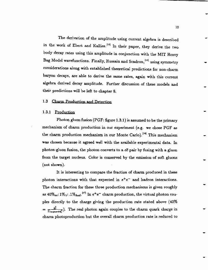
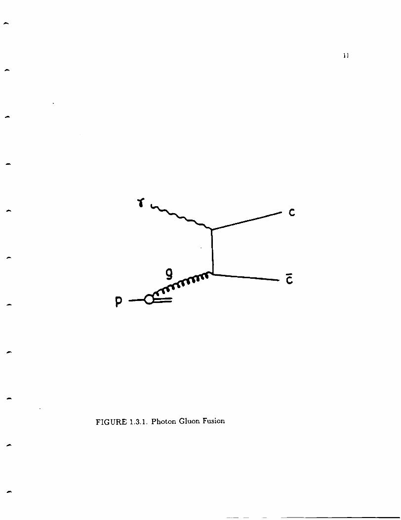
Photon gluon fusion (PGF: figure 1.3.1) is assumed to be the primary
mechanism of charm production in our experiment (e.g. we chose PGF as
the charm production mechanism in our Monte Carlo). 11111 This mechanism
was chosen because it agreed well with the available experimental data. In
photon-gluon fusion, the photon converts to a cc pair by fusing with a gluon
from the target nucleus. Color is conserved by the emission of soft gluons
(not shown).
It is interesting to compare the fraction of charm produced in these
photon interactions with that expected in e+ e- and hadron interactions.
The charm fraction for these three production mechanisms is given roughly
as 40%ee: 1%1 : .1%had· 117J In e+e- charm production, the virtual photon cou
ples directly to the charge giving the production rate stated above ( 40%
= E· 9~ 2 ). The real photon again couples to the charm quark charge in ••q.car•9'i
charm photoproduction but the overall charm production rate is reduced to
-
-
-
-11
-
-
-
- c
-c
- p
-
-FIGURE 1.3.1. Photon Gluon Fusion
-
-
12
the 1 % level by the high mass of the charm quark.* Hadroproduction suffers
relative to photoproduction because, in gluon-gluon fusion (the ha.dronic pro
duction mechanism) the gluon coupling to the charm quark depends not on
the quark charge but on the gluon momentum distribution which is skewed to
low X121
(Xis the fraction of the particle's momentum carried by the gluon).
Naively, e+e- production of charm would be the favorite method
of charm production, with hadroproduction the least favorite. The abso
lute production rate in real photon charm production is, however, orders of
magnitude higher than e+ e- production because of the higher effective lu
minosity in the photon experiment (.Ce+e- "' 1 pb-1 /day 11' 1 : .CEs91 "' 103
pb-1 /day). Hone were able to control the increased backgrounds inherent
in the real photon charm production, this increased rate of production could
be put to advantage. Charm particle lifetime studies would be of particular
interest since the boost the particle receives in the fixed target interaction
is much greater than that received in the e+e- interaction (P charm "' 3
GeV/c2 (e+e-) typically: 20 GeV/c2 < Pclaarm < 140 GeV/c2 {fixed target)
in E691 ). Charm decay distances (="'(CT) would therefore be much greater
in the fixed target interaction and hence measured more easily.
1.3.2 Detection
Detecting the charm signal produced in the experiment presents
many problems. The first problem one notices is the low branching frac
tions of all charm decay modes. Typical values of 5% (compare this to the
decay Ao - p7r, with the branching fraction of"' 64%) imply that, for spe
cific signals, we access not 1% of the total cross section, as discussed above,
* PGF productions crossections peak for low values of M2 (::: mass of the created particle pair). IHI Low m888 quark photoproduction is therefore enhanced relative to charmed quark production.
-
-
-
-

-
-
-
-
-
-
-
-
13
but .05%. More worrisome still are the large number of possible track com
binations in a typical fixed target event (the combinatorics). This problem
is aggra\·ated not only by the high track multiplicity (5-10) associated with
these events but by the dominant non-charm event fraction as well. Given
these considerations, the efficiency with which we reconstruct a given charm
decay mode turns out to be on the order of 5%. Thus, for a charm decay
with these characteristics ( 5% branching fraction; 5% efficiency :::::} strong
candidate mode), only 2.5 x 10⁻⁴ of the recorded events would produce a re
constructed charm decay in this channel. Vle would therefore need to record
108 events to tape to reconstruct 2500 of these charm decays.
Recording 108 events does not solve the problem however. The goal
of the experiment is not just to produce large signals but to produce large
significant signals. The background, which is a product of the combina
torics discussed above, must then be separated from the signal by some
means, and removed. From the advent of charm physics, 1191 identifying and
isolating the charm vertex from the production vertex was considered the
most fertile signature available with which to identify charm signals. The
decay distance in the beam direction of a typical charm particle would be on
the order of millimeters for a fixed target experiment, given CTcharm "" lOOµm
( = proper decay length of the charm particle). For decay lengths of this size.
one would need transverse resolution of < 25µm from the vertex detector
(section 3.2) to obtain significant separation of the charm and production
vertices.
The fact that the charm quark decays predominantly to a strange
quark is another well known signature for charm. This tendency (expressed
quantitatively with the Cabbibo angle) implies that a strange particle is

14
normally among the charm particle's decay products. An effective parti
cle identification scheme {section 3.5) that would allow one to separate the
kaons and protons in these charm decays from the prevalent pions in the
background events would lead to a large reduction in the combinatorics and
provide a powerful background filter for the analyses of the charm decay
modes.
The history of experimental fixed target charm physics teaches us one
thing; charm signals have very large background levels. The e+ e- experi
ments succeeded because they had manageable background levels to begin
with. Fixed target experimenters had to learn how to manage their much
larger background levels by exploiting the charm signatures discussed above.
1.4 A Brief History of Experiment E691
Each of the experimental refinements outlined in the previous section
{a 108 event data sample, a high resolution vertex detector, superior particle
identification) was realized by experiment E691. A critical study of the pre
vious run, experiment E516, led to numerous important improvements in the
spectrometer. The crucial improvement was the inclusion of the silicon mi
crostrip detector (see section 3.2) which provided an additional background
suppression of two orders of magnitude in the analysis of the charm decay
modes. This enabled E691 to do fixed target charm physics effectively.
The experiment ran from late April 1985 until the end of August 1985
during which time ,...., 108 events were written to tape. It should be noted
that these events were taken with a transverse energy trigger that enhanced
charm about 2.5 to 1 with respect to normal hadronic trigger events (see
section 3.9). The analysis presented in this thesis includes the entire data
set.
-
-
-

-
-
-
-
-
CHAPTER 2
THE PROTON AND PHOTON BEAMS
The study of the decay properties of charm particles was the goal of
experiment E691, with an emphasis on lifetime and branching ratio determi
nation. The hardware involved in the experiment was designed to maximize
the production and optimize the detection of these charm particles. The deci
sions involving the hardware were constrained by competing considerations.
Upstream of the photon-nucleon interaction, the beam flux, the electron and
photon beam energy, and the beam purity were of most concern. Down
stream of this interaction, accepting, identifying, and resolving the positions
and momentum of the charm particle decay products, and rejecting non
charm background, were the primary concerns. The structural form and the
function of each element of the beamline and the detector will be discussed
as will the physical principles governing these devices.
2.1 The Proton Beam
The proton beam reached 800 Ge V through a five stage process.
First, hydrogen gas was ionized. The protons were then, in turn, accelerated
to 750 KeV/c2 by a Cockroft-Walton, to 200 MeV/c2 by a linac, to 8 GeV
by a booster ring, to 150 GeV by the Main Ring, and finally, to 800 GeV by
the Tevatron which is a strong-focusing synchrotron using superconducting
magnets. During the Main Ring acceleration stage, the protons were grouped
into 'buckets', 2 ns in length and 19 ns apart, and the beam maintained this
time structure at all subsequent stages. The protons were extracted from the

16
Tevatron during a 22 second spill and a new spill started every 65 seconds.
Upon extraction, a septum split the beam between 3 beamlines; Meson, Neu
trino, and Proton (fig(2.1.1). The Proton beam was shared between 3 more
beamlines; PWEST, PCENTER, and PEAST, where PEAST contained the
photon beamline used in this experiment. On average, PEAST received 20%
of the 1013 protons generated in a typical Tevatron spill. Figure 2.1.1 shows
the layout of the fixed target beamlines at Fermilab.
2.2 The Photon BeHJD
Conversion of this proton beam into a photon beam was handled in
the following manner (fig 2.2.1). 1201 The PEAST proton beam was directed
onto a 30 cm berylium target (a) where secondary particles, charged and
neutral, were created. The charged particles were swept into a beam dump
by a magnet (b ), while the neutral particles, mainly K2s, neutrons, and
photons from 7r0s, continued on. The photons impacted a lead radiator (c)
and converted to electron-positron pairs. At this point, we chose the electron
beam which became the source, via bremstra.hlung, of the final photon beam.
An electron beam was chosen because, knowing the energy of this beam,
and measuring the post-bremstra.hlung electron energies (see section 2.3), we·
could derive the photon energy (i.e. tag the photon). The beam energy was
selected using a set of adjustable magnets and horizontal collimators while
the dispersion of the beam was determined by the size of the collimator
openings. This beam was transported to the Tagged Photon Laboratory
where it impacted a tungsten radiator (d) and produced a bremstrahlung
photon (with N,. "" 1/E,. 1211 ). The photon beam spot was then centered on
the experimental target and was easily contained within the (2.5cmx2.5cm)
transverse dimensions of the target.
-
-
-
-
-

.,
MESON AREA .. ~~~-qr.:..---
® To,o•' - - Test seom
t.auUipoftic\e spectfom•'''
MP po\. p,oton aeom \5' Bubble Chomb•'
Brood aond aeom
count•' facilities
..... _,

266----
263-----249------
tr beam
Target
e- Dump
I st bend• 19.677mr 2nd bend: 7.111 mr 3rd bend• 18.859mr
Tagging Hadascape
Horizontal Bend Vertical Steering
Quad. Doublet
Vertical Steering
Horizontal Bend
Vertical Collimator Horizontal Collimator
Horizontal Bend Horizontal Collimator
Vertical Steering
Quad. Doublet Vertical Collimator
© Converter (Pb, .32cm thick)
Proton Dump
(D) Dump Magnet
0 ~------- @ Be Target (30cm langl (meters)
p
FIGURE 2.2.1. PEAST Beamline
18

-
-
-
-
-
-
-
-
-
-
19
To ensure the purity of the beam, the pion and muon contamina
tion had to be minimized. The lead radiator was .5 radiation lengths and
.02 interaction lengths thick so that the pion contamination introduced at
this point by neutral hadronic interactions was small. The pions that were
produced here had a much higher average Pt than the electron beam so,
using tight vertical collimators in the beamline (fig 2.2.1), the pion contam
ination was reduced below the 1 % level (the characteristic collinearity of
the electron-photon system is exploited many times in the hardware design).
The muon halo on the photon beam, which originated at the charged parti
cle beam dump, was minimized by building the electron beamline 7 meters
offiine (,..., 7 mr offset) from the original direction of the PEA ST proton beam.
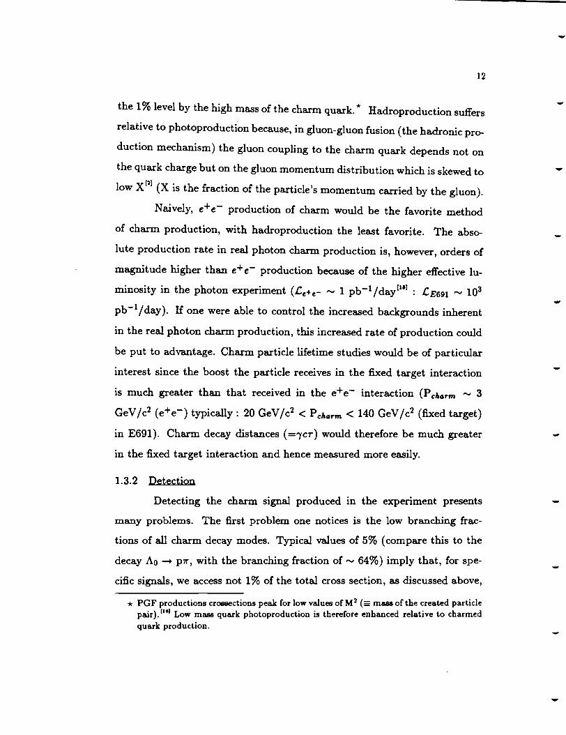
The choice of the beam energy, the beam flux and the tagging radia
tor then had to be made. A high electron beam energy was desirable because
charm production cross sections rise significantly as the photon beam energy
rises. The beam flux, on the other hand, decreases with the beam energy
(fig 2.2.2) and thus had to be chosen in congress with the energy. All three
choices affected our ability to tag the photon.
A radiator of .2 radiation lengths was chosen to suppress double
bremstrahlung by the electron and pair production by the interaction photon,
as both these effects made tagging the photon difficult. The choice of beam
energy, 260±8.5 GeV, was motivated mainly by a desire to maximize the
mean photon energy while maintaining sufficient flux. With this energy and
radiator, the photon flux we obtained (,..., 107 /'/spill> 80 GeV /c 2 ) produced
enough interactions in the target to saturate the E691 data aquisition system
(DA); ,..., 2200 events/spill with 30% deadtime (see section 4.2).
A. z ' • z
. 0.2
20
0.6
FIGURE 2.2.2. Ne/Np = Fractional Electron Yield; Ee/Ep = Fractional Electron Energy. E691 operated at Ee/Ep = 250/800 with an electron yield of-2x10-s.
-
-
-
-
-
-
-
-
-
-
21
With regards to tagging the photon beam, this beam flux implied
that only 5% of the beam buckets entering the Tagged Photon Laboratory
contained electrons and only 10% of these contained more than one. Multi
electron buckets were therefore not a serious problem for the tagging system
since these buckets produced more than one photon only a few percent of
the time. Double bremstrahlung in single electron buckets was also kept
within reasonable limits, occurring ......, 15% of the time. An attempt was
made to address this problem (see section 2.3). In any event, with nearly the
maximum electron beam energy ( 300 Ge V = maximum energy transportable
by the TPL beamline), we saturated our DA and kept double bremstrahlung
and pair production in the radiator at acceptable levels.
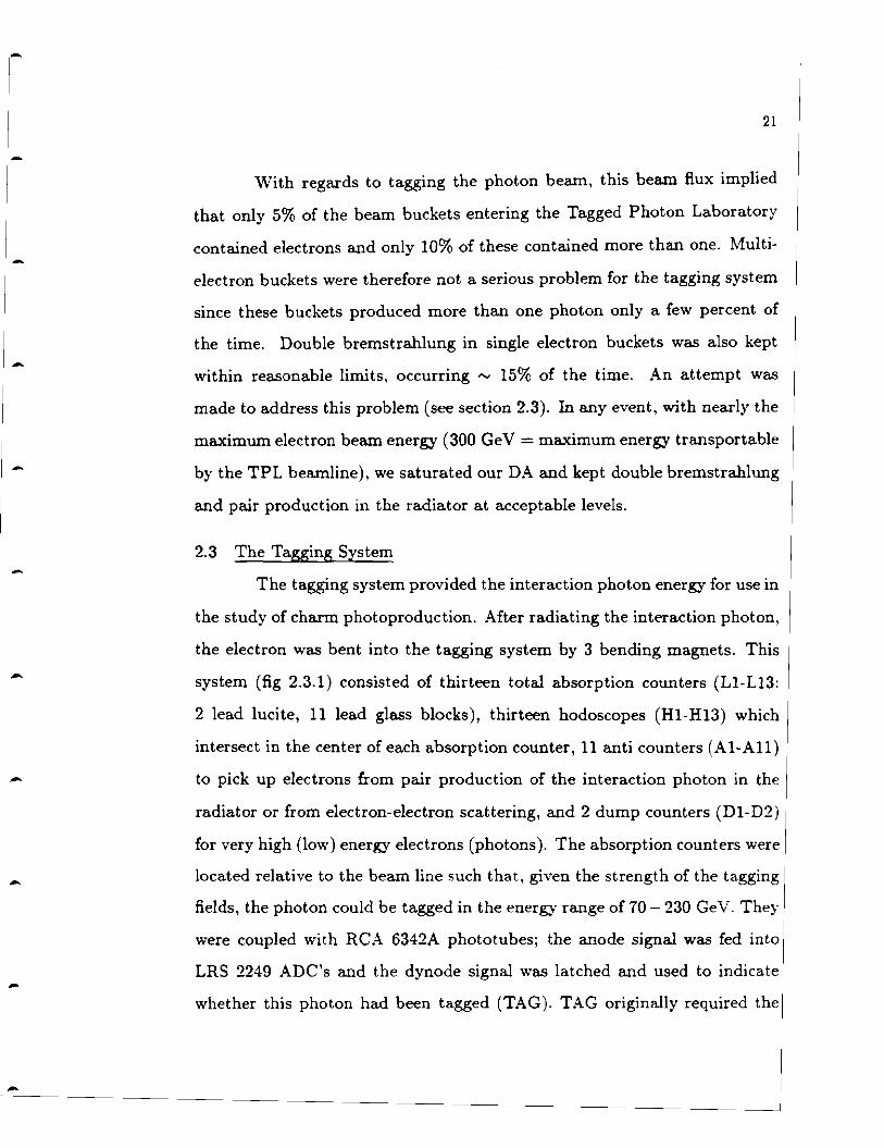
2.3 The Tagging System
The tagging system provided the interaction photon energy for use in
the study of charm photoproduction. After radiating the interaction photon,
the electron was bent into the tagging system by 3 bending magnets. This
system (fig 2.3.1) consisted of thirteen total absorption counters (Ll-113:
2 lead lucite, 11 lead glass blocks), thirteen hodoscopes (Hl-H13) which
intersect in the center of each absorption counter, 11 anti counters (A 1-A 11)
to pick up electrons from pair production of the interaction photon in the
radiator or from electron-electron scattering, and 2 dump counters (Dl-02)
for very high (low) energy electrons (photons). The absorption counters were
located relative to the beam line such that, given the strength of the tagging
fields, the photon could be tagged in the energy range of 70- 230 GeV. They
were coupled with RCA 6342A phototubes; the anode signal was fed into
LRS 2249 ADC's and the dynode signal was latched and used to indicate
whether this photon had been tagged (TAG). TAG originally required the

19m
Experimental Apporotus
A9
A8
A7 A6
A4 A3
ift'I"""~--....- Muon Counters Concrete Shielding
~=~i----1.L ,- Beam Dump -1111--wi---+'~ Hodo1eope (HI· H13)
ond Counter Array Lt· L2 L3-L8 L9-L13
1----~"-Voeuum V1111l
Tagged Photon Building Woll
>-Togging Magnets
:---++----- Anti Counters m..;..;.;...--w.---- Rod iator
t .-
FIGURE 2.3.l. The Tagging System
22
-
-
-
-
-
-
-
23
logical AND of two adjacent hodoscope elements and the absorption counter
directly behind it. However, the hodoscopes proved inefficient and were
remoYed from the TAG logic for the last half of the experiment (see section
3.10).
The final element of the tagging hardware was the C-counter. This
total absorption counter was placed after the last set of drift chamber planes,
directly downstream of the target. It's purpose was to measure the energy
of the non-interacting photons produced by multiple bremstrahlung in the
radiator. The final photon energy would be given as
E-, = Ebeam - ErAG - Ee
Due to the high fiux of particles into this counter during the run, however,
the more accurate measure of photon energy was simply,
E-, = Ebeam - ErAG· (2.3.1)
Calibrating the tagging system was a three step process. First, the
C-counter was calibrated by turning off the tagging magnets and removing
the target. Since the electron beam energy was known, the ADC counts per
Ge V in the C-counter was easily obtained (the linearity of the C-counter was
tested with double electron buckets). Turning the tagging magnets back on
but leaving the target out, we then calibrated the tagging system, with the
photon energy measured by the C-counter,
Er AG = Ebeam - Ee; Ee = E-, (2.3.2)
Minimizing (for many events),
13
x2 = L(ErAa - 9iADCi)2
i=l
we obtained the gains, gi, of the phototubes.
24
Finally, the electron beam energy itself was calibrated using elastic
p (and independently, '11) production ("YP-+ pX; p-+ 1r+1r-). A check for
energy deposition in the calorimeters and for high momentum tracks was
made to ensure that this interaction was elastic. To good approximation,
with the invariant mass of the two pions restricted to the p mass region. An
in depth discussion of this procedure can be found elsewhere. 1221
-
-

-
-
-
-
-
-
-
-
-
-
CHAPTER 3
THE DETECTOR
The Tagged Photon Laboratory (TPL) spectrometer is a two mag
net spectrometer with large acceptance, good mass resolution, good particle
identification using Cerenkov counters, muon detectors, and electromagnetic
and hadronic calorimeters, and very good secondary vertex detection using
silicon microstrip detectors. The spectrometer is shown in figure 3.0.1. Each
component of this detector is discussed below.
3.1 The Target
In choosing a target for the photon beam, we had to choose both the
target material and the target size. The charm cross-section is ex A and the
dominant background for a photon beam is pair production which is ex: Z2' so
we had to minimize the ratio Z2 I A. The material with the smallest value of
Z2 I A is deuterium, but, to obtain sufficient interaction rates with liquid D~,
the target would have had to be on the order of a meter in length. This poses
some serious problems, because, for a one meter target, angular resolution
and multiple scattering would dominate the resolution of the SMD's for most
tracks associated with an interaction vertex (ideally, the intrinsic resolution
of the SMDs provides the dominant contribution to the overall resolution). In
addition to this, the charged track acceptance drops as the distance between
the interaction vertex and the SMDs increases. Given these considerations,
we chose a 5cm long berylium target. With this target, we achieved sufficient
interaction rates, the multiple scattering and angular resolution contributions

TAGGED PHOTON SPECTROMETER E691
SMO"S
CALORIMETERS HAORCINIC =--
EM CSLICI~ ~
DRIF'T CHAMBERS '\
04 ---------COUNTERS
C2 ~
DRIFT CHAMBERS ----03,03'
MAGNET

-
-
-
-
2i
to the resolution were small, and the charged track acceptance was good. The
tradeoff is that (Z2/A)Be '.:::::'. 4x(Z2/A)D2 which was acceptable.
The frequency with which the photons interact a second time (sec
ondary interactions) is also dependent on the choice of target length and
material. These interactions are ~ A 213 so lowering this rate would have
meant using a shorter target and, thus, lowering the primary interaction
rate. The primary interaction rate could have only been made up with a
higher photon beam flux which, as discussed earlier, meant a lower electron
beam energy and a lower average photon spectrum energy. Thus, in order to
maintain a constant primary rate of interaction, the average photon energy
would have to drop as the target size decreased. The target chosen above
was ,..., .1 interaction lengths which proved to be a satisfactory compromise
choice implying a secondary interaction rate ,....., 5%.
The B-counter (not shown in the figure 3.0.1) was a small (2.5cm x
2.5cm active area) scintillation counter set directly downstream of the target.
It was thin, to minimize secondary interactions and multiple scattering, and
its phototube and base were designed to handle high rates. It was used to
indicate that an interaction had occurred and it's threshold was set at just
above 1 minimum ionizing particle (MIP). It's primary function was to set
the timing of the experiment and to be used as an element in the trigger.
3.2 The Silicon Microstrip Detector
The purpose of the silicon micros trip detectors ( SMD) was to detect
the small separation {a few mm) between the interaction and the charm decay
vertices. As mentioned earlier, charm particles decay weakly so transverse
decay distances on the order of lOOµm are expected, with CT ,....., lOOµm.
Our system of 9 SMD planes (see table 3.2.1) had a pitch of 50µm and,

28
thus, an intrinsic transverse resolution of 14µm per plane1231 (experimentally
measured resolution 16µm 1241
) which was sufficient to isolate the secondary
vertex. Requiring a significant separation between the cha.rm decay and
interaction vertices in the data analysis would typically drop background
levels by two orders of magnitude.
Table 3.2.1: Characteristics of the Silicon Microstrip Detectors
Triplet 1 2 3
Size 2.6cmx2.6cm 5.0x5.0 5.0x5.0
pitch 50µm 50µm 50µm
strip width 300µm 300µm 300µm
working strips/planE 512 768 1000
z(central) 6.684cm 14.956cm 23.876cm
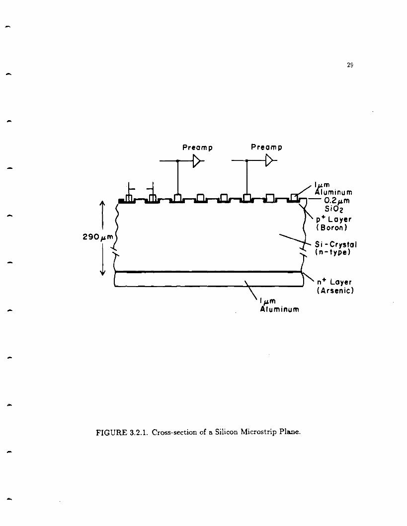
Figure 3.2.1 shows a cross-section of a silicon microstrip plane. The
structure is that of a P-1-N diode1:u1 , with boron implanted in strips on the
upper surface, arsenic implanted on the lower surface, and aluminum de
posited on top of these layers to provide the electrical connection. Applying .
an electric field to this plane creates charged layers on either side of the P-1
junction because the conduction electrons in the undoped silicon drift into
the P + (boron) region until the field created by the charge imbalance pre
vents further migration. The positively charged layer is called the depletion
zone because this migration depletes the conduction band in the silicon. The
entire undoped silicon wafer can be depleted by applying a 'reverse bias' volt
age of about 90V across the microstrip plane .. During the operation of the
detector, this wafer must be fully depleted to prevent the holes from recom
bining with conduction band electrons as this would reduce the signal. Once
-
29
Preamp Preamp
-tim luminum
I -o.2"'m
- Si Oz p+ Loyer (Boron)
290 "'m
1 Si-Crystal (n-type)
n+ Layer (Arsenic)
- '"'m Aluminum
-
-FIGURE 3.2. l. Cross-section of a Silicon Microstrip Plane.
-
-

30
fully depleted, any electron-hole pair created in the silicon is efficiently swept
out by the field across the plane; the holes to the P+ layer, the electrons to
the N + layer (which is held at ground). The passage of a MIP through the
depleted microstrip plane created - 24000 electron-hole pairs and the signal
picked up by the strips (the hole cloud) was collected in less than lOns with
a typical transverse extension of lOµm.
The size of the detectors and of the output signals they generated
presented major experimental difficulties. With 6840 instrumented channels,
the volume increase in hardware from the microstrips to their CAMAC read
out was greater than 3 orders of magnitude. To complicate things further,
the signals from the SMD's were - 4 femtocoulombs so everything had to be
shielded and efficiently grounded. To be specific, the preamplifier assigned to
each instrumented strip had to be positioned close to that strip to minimize
the capacitance and, thus, the noise introduced at this stage. In addition
to this, the rotational position of each detector plane, as well as its posi
tion with respect to the beam axis, had to be extremely well defined to take
full advantage of the spatial resolution of this detector. Finally, the leak
age currents across these planes, caused by noise induced electron-hole pair
generation in the silicon, 1211 had to be closely monitored. Fortunately, these
currents remained under control during the run due to proper preparatory
care of the detectors.
The 9 SMD planes were ordered into 3 triplets of 3 views each; X, Y,
and V ( +20.5° to X). Each triplet was located in a light tight, rf shielded box
and positioned with a plane to plane precision of 12µm and relative rotational
offset precision of .Smr. The preamps were attached directly to the rf boxes
and generated outputs of,..,, lmV. This signal was transmitted to the readout
-
-

-
-
-
-
-
-
-
31
system by 4m shielded cables of 9 channels each; 4 channels carrying signal
and the 5 alternate channels connected to ground to reduce cross-talk. The
signals were fed into 8 channel Nanosystem 5710/810 M\VPC shift register
cards which were discriminated at ,...., .4m V and read out serially by CAMAC.
v.rith this discriminator level and a 50ns gate for the event, we averaged 1
noise hit per plane per event while the track detection efficiency at large
angles dropped by only 20% (transverse extent of signal here > 25µm). In
general, the per plane track detection efficiency was ,....., 90%. Further details
on the construction and operation of this detector can be found elsewhere. !2
•1
3.3 The Drift Chamber System
The drift chamber system provided additional track position infor
mation and in conjunction with the magnets, determined the track momenta.
There were 35 drift chamber planes grouped into 11 assemblies, each assem
bly generating a space point (triplet) for each track. These assemblies were,
in tum, grouped into 4 drift chamber stations with which we could obtain a
measurement of the track direction and position at particular locations along
the spectrometer and thus determine its momentum (see table 3.3.1).
In a typical drift chamber plane, the grounded sense wires alternate
with field shaping wires which are held at high negative voltage (- -2 kV).
This plane is sandwiched between two planes of wires all of which are set
to high negative voltage (- -2.4 kV). The electric field one obtains in the
region bordered by the field shaping wires and the high voltage planes is
approximately constant in magnitude and direction, except near the sense
wire; this region is called a cell. For certain gas environments (ours: 50-50
argon/ethane + 1.5% ethanol to quench sparks) and high voltage settings,
the electrons freed in this cell by the passage of a charged particle will drift
32
to the sense wire with an approximately constant drift velocity which is
reasonably insensitive to small voltage changes. Thus, given the measured
drift time .6t and the drift velocity VtJri/ti a reliable measure of the distance
from the impact point of the ionizing particle to the sense wire can be made , ddri/t = v drift x .6t, and position resolutions of"' 300µm can be achieved.
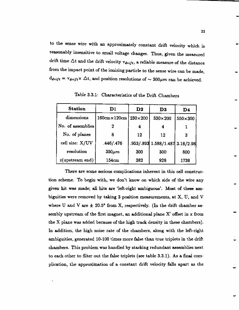
Table 3.3.1: Characteristics of the Drift Chambers
Station Dl D2 D3 D4
dimensions 160cmx120cm 230x200 330x200 550x300
No. of assemblies 2 4 4 1
No. of planes 8 12 12 3
cell size: X/UV .446/.476 .953/.89~ 1.588/1.487 3.18/2.98
resolution 350µm 300 300 800
z(upstream end) 154cm 382 928 1738
There are some serious complications inherent in this cell construc
tion scheme. To begin with, we don't know on which side of the wire any
given hit was made; all hits are 'left-right ambiguous'. Most of these am
biguities were removed by taking 3 position measurements, at X, U, and V
where U and V are ± 20.5° from X, respectively. (In the drift chamber as
sembly upstream of the first magnet, an additional plane X' offset in x from
the X plane was added because of the high track density in these chambers).
In addition, the high noise rate of the chambers, a.long with the left-right
ambiguities, generated 10-100 times more false than true triplets in the drift
chambers. This problem was handled by stacking redundant assemblies next
to each other to filter out the false triplets (see table 3.3.1). As a final com
plication, the approximation of a constant drift velocity falls apart as the
-
-

-
-
-
-
-
-
-
-
33
signal electrons approach the high fields at the sense wire. This limited our
ability to resolve the impact point with the simple linear equation for ddrift
given above (on a positive note, the avalanche caused by the signal electrons
in this region would typically amplify this signal into the convenient lm V
range). These and other problems are discussed in detail elsewhere1i
6J •
To obtain ddrift from the hardware, we need Vdrift and 6t, as stated
above. The time actually measured by the Time to Digital Converter (TDC)
connected to this sense wire is 6 t' = T atop - Ta tart. T start is the time at which
the signal from the sense wire reaches the TDC and T stop is generated by
the trigger logic such that any sensible T atart is before T stop· For our case
then,
6t = (Tstop - Tatart(O)) - !:::.t'
with T ,,tart(O) equal to the time measured by the hardware when a track hits
the sense wire (it is determined by cable lengths, electronic response, and
the z-position of the cell in question).
In the drift chamber vernacular we get;
(T,,iop - T,,tart(O)) = Trel +Tabs·
Tab,, is the time assigned to each plane to account for the intrinsic time
differences between the planes while T rel accounts for the cell to cell time
differences by measuring the response of the cells in this plane relative to
Tab". Knowing the constant time offsets between the planes a.nd between the
cells in each plane, we can obtain the physically pertinent quantity, the drift
time. Finally,

34
(3.3.1)
The LRS 4290 system is able to account for Tre1 on-line by pulsing the planes
d . h [21) • unng t e run . Therefore, the value we wnte to tape is,
(3.3.2)
This distribution is shown in figure 3.3.2 where t2=T0 6a, t=O=Tatop, and
t1=time measured from the edge of the cell.
The muon halo, discussed earlier, provided a clean source of tracks
with which to calibrate not only the T 0 6., but Vtlri/h and the chamber align
ment offsets as well1211 • With 6t and Vtlri/t in hand, we obtained dtlri/t and
could then proceed to determine the positions and momenta of the tracks
throughout the spectrometer. The drift chamber planar efficiencies were
-903.
As stated earlier, the eleven assemblies are split up into 4 drift cham
ber stations so that we could obtain a reliable measure of the direction and
positions of the tracks. Dl, assisting the SMDs, pinned down the tracks
upstream of the first magnet, Ml. D2's four assemblies provide the tracking
between Ml and the second magnet, M2. D3 provides the final particle tra
jectories and positions with an assist from D4 (which had limited usefulness
because charged particles back scattered from interactions in the SLIC (sec
3.6) reduced this chamber's position resolving capabilities1221 ). We obtain
the momentum using the relation,
-
-
...
-

-
-
-
35
400
300
• • ... -c l&J 200 ... 0
0 z
100
0"'--'-~~-'---1...&.-'-...... ---'-....... -----_..~..-. ........ --~~--o t 100 200
I 300
Time (ns)
FIGURE 3.3.2. TO Distribution. The dashed curve represents the response or a perfect cell with tz ==TO ABS and t1 =outer edge of cell. The histogram represents the response or a physical cell where non-linear drift velocities, etc. have affected the shape of the distribution.

.3f B ·di p = 68 ,
36
(3.3.3)
where 68 is the measured change in trajectory from one side of a magnet to
the other. The momentum resolution is given by
(3.3.4)
where
(3.3.5)
with Uz the error in the drift chamber position measurement, N the num
ber of planes, and L their separation. We see that momentum resolution
improves with increasing field and increased redundancy. For E691, the
momentum resolution for tracks that penetrate both magnets was 6p/p ~
.05p(GeV /c2 )% + .5% 1291 where the last term is due to multiple scattering.
3.4 The Magnets
The characteristics of the E691 magnets are given in table 3.4.1.
They were used not only to derive track momenta but to sweep low energy
e+e- pairs out of the spectrometer and to increase charged track separation
(implying better tracking in the drift chambers downstream of them). The
fields were measured using a zip-track which employed a small ca.rt with 3
small perpendicular wire coils. It ran on an aluminum track which pen
etrated both magnet apertures allowing the coils to test the field at well
defined values of (x, y, z). These values were written to tape and then fit
with orthogonal polynomials consistent with Maxwell's equations. The field
-
-
-

-
-
-
-
-
-
-
-
37
strengths used by E691 are in the table. The quality of the map was measured
by studying the K,, -+ 71'71' mass and comparing its average value to the
Particle Data Group 121 value.
Table 3.4.1: Characteristics of the TPL Magnets
Magnet Ml M2
entrance 154cmx73cm 154cmx69cm
exit 183cmx91cm 183cmx86cm
length 165cm 208cm
JB·dl -.071 T-m -1.07 T-m
Pt kick 0.21GeV/c2 0.32GeV/c2
3.5 The Cerenkoy Counters
The Cerenkov counters were the primary responsibility of the Col
orado group. It was my responsibility to maintain them during the experi
mental run and therefore this detector will be discussed in more detail than
the other detectors in the spectrometer. They were used to identify the pro
tons and charged kaons from among the more prevalent pions in the data,
for the presence of these less copiously produced particles is a signature of
charm particle decays. 1111
A particle exceeding the speed of light in a given medium emits
Cerenkov radiation, 127] implying that the momentum at which the radiation
is first produced is,
,..., me Pth = -J2e
(3.5.1)
with e=n( A )-1 and n( A )=index of refraction of medium. This is called the
38
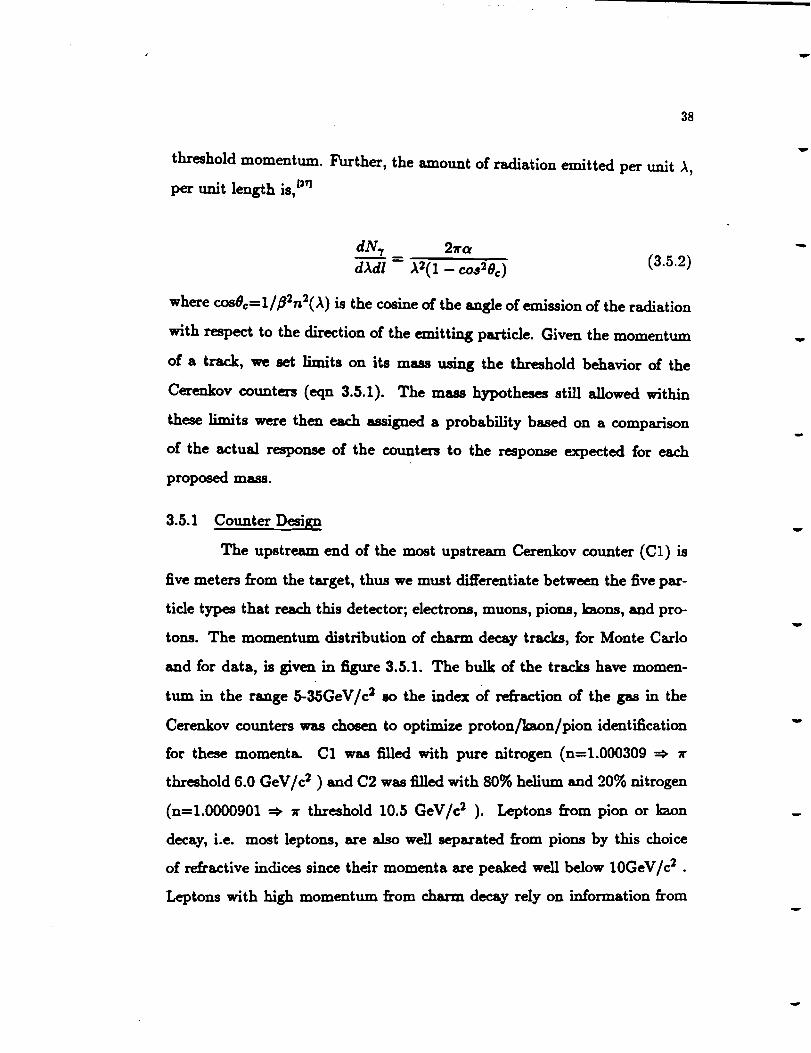
threshold momentum. Further, the amount of radiation emitted per unit .X,
per unit length is, l27l
dN-, 27ra d).dl = ).2(1 - cos28c) (3.5.2)
where cos8c=l/ ,82n2().) is the cosine of the angle of emission of the radiation
with respect to the direction of the emitting particle. Given the momentum
of a track, we set limits on its mass using the threshold behavior of the
Cerenkov counters (eqn 3.5.1). The mass hypotheses still allowed within
these limits were then each assigned a probability based on a comparison
of the actual response of the counters to the response expected for each
proposed mass.
3.5.1 Counter Design
The upstream end of the most upstream Cerenkov counter (Cl) is
five meters from the target, thus we must differentiate between the five par
ticle types that reach this detector; electrons, muons, pions, kaons, and pro
tons. The momentum distribution of charm decay tracks, for Monte Carlo
and for data, is given in figure 3.5.1. The bulk of the tracks have momen
tum in the range 5-35Ge V / c2 eo the index of refraction of the gas in the
Cerenkov counters was chosen to optimize proton/kaon/pion identification
for these momenta. Cl was filled with pure nitrogen (n=l.000309 ~ 7r
threshold 6.0 GeV /c2 ) and C2 was filled with 80% helium and 20% nitrogen
(n=l.0000901 ~ 71" threshold 10.5 GeV /c2 ). Leptons from pion or kaon
decay, i.e. most leptons, are also well separated from pions by this choice
of refractive indices since their momenta are peaked well below lOGeV /c2 •
Leptons with high momentum from charm decay rely on information from
-
-
-

-
-
-
-
- .
-
-
39
the SLIC (sec 3.6 ) and the muon wall (sec 3.8) to augment the Cerenkov
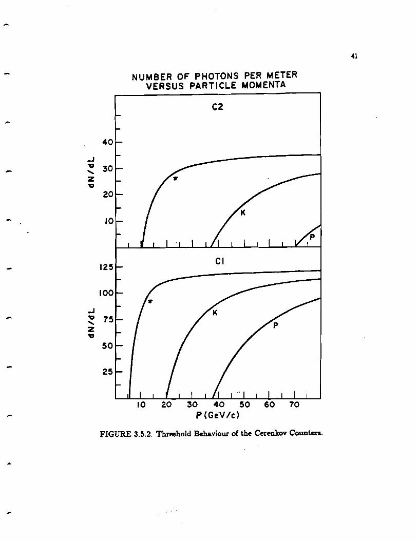
information. The threshold behavior of the two Cerenkov counters for the
three prevalent particle types is illustrated in figure 3.5.2.
The Cerenkov counters are shown in figure 3.5.3 and their parameters
described in table 3.5.1. The design specifications of the two counters are
straight forward. The length of both counters was chosen so that, allowing for
the index of refraction of the gas, absorption in the gas, reftectivities, and the
quantum effidencyr-1 of the phototube, approximately fifteen photoelectrons
would be obtained in each. The Cerenkov light is emitted, as stated earlier,
at an angle cos(Bc:) ={1//J2n2p.)) with respect to the particle direction, and
isotropically in the angle t;. The radiation pattern for a constant velocity
particle is, therefore, disk-like with radius = L x tan8c (where L = length
of the Cerenkov counter). This radiation pattern hits a wall of spherical
mirrors at the counter's downstream end. The mirror walls in Cl and C2
(with 28 and 32 mirrors respectively) are shown in figure 3.5.4.
Table 3.5.1: Characteristics of the Cerenkov Counters
Counter Cl C2
length 3.7m 6.6m
No. of cells 28 32
gas N2 80% He+ 20% N2
refractive index 1.000309 1.0000901
radius of light pattern( max: 8.4cm 8.7cm
~threshold 6.0GeV/c2 10.5GeV/c2
z(mirror plane) 866cm 1653

40
CHARGED PARTICLE MOMENTUM SPECTRUM
900
800 --- MONTE CARLO - DATA
en 700 I I
~ ..! I .
u I I ct 600 I
a:: I I
I-I I
"" 500 I ._
0
a: 1£.1 400 m ~ :::> z 300
200
100
0 20 40 60 80. 100 P(GeV/c)
FIGURE 3.5.1. Predicted and Observed Momentum Spectrum of 2-Magnet Tracks.
-
-
-
-
-
-
-
-
-
-
-
-
-
-
40
_J
~ 30 ...... z ~
20
10
125
100
_J ~ 75 ...... z ~
50
25
NUMBER OF PHOTONS PER METER VERSUS PARTICLE MOMENTA
C2
Cl
I 0 20 30 40 50 60 70 P(GeV/c)
FIGURE 3.5.2. Threshold Behaviour of the Cerenkov Counters.
41

DOWNSTREAM CERENKOV COUNTER ICZJ
UPSTREAM CERENKOV COUNTER ICU
lltltltOlt STltlNG AOolUSTl:ltS
WINSTON CONI: l"OltTALS
42
(A)
(B)
FIGURE 3.5.3. Schematic of the Cerenkov Counters. Cl is shown in (A) and C2 is shown in (B).
-
-

-
43 -
-C1 MIRROR ARRAY
- 13 9 2 10 14
II 7 5 3 I 4 6 8 12
- 25 21 19 17 15 18 20 22 26
27 23 16 24 28
-C2 MIRROR ARRAY
15 II 2 12 16
-13 9 7 5 3 I 4 6 8 10 14
29 25 23 21 19 17~0 22 24 26 30
- 31 27 18 28 32
-FIGURE 3.5.4. Mirror Patterns of the Cerenkov Counters.
44
The mirror segmentation pattern was chosen, using Monte Carlo
techniques, to reduce the chance of two tracks throwing light on the same
mirror, since good Cerenkov identification requires a unique knowledge of
the light produced by each track. The minimum mirror size allowed in this
segmentation scheme "' contained the light pattern thrown by a centered high
momentum track (maximum radius of Cerenkov light pattern= 8.4cm(Cl)
or 8.7cm(C2)). With this mirror arrangement, the chance that two (or more)
tracks would radiate any one mirror in Cl or C2 was < 103. (29J
The mirrors were slumped by industryl•I and coated at the Univer
sity of Colorado. Wmdow pane glass was used for the mirrors in both Cl
(2.4mm thick) and C2 (3.2mm thick) and was slumped with a focal length of
190±20cm. Mirrors with major surface distortions were not accepted. The
aluminum was deposited on the mirror at a deposition rate of"' 35 A/sec
for 30sec at "' 10-6 Torr and was overcoated with a 250A layer of MgF2 to
prevent oxidation of the aluminum surface. Refiectivities were then tested at
small waYelengths (2525A) since, for Cerenkov radiation, N,. ex 1/')..2 (see eqn
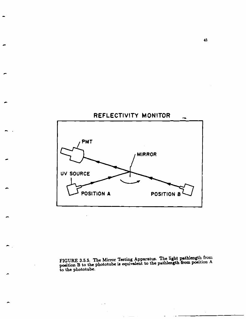
3.5.2). The apparatus used to test these reftectivities is shown in fig 3.5.5. To
begin the test, an ultraviolet light source, equipped with a low wavelength
filter, was placed in position (A) and the phototube output was recorded.
The source was then placed at position (B), the mirror was removed, and
the phototube output again recorded. This second measurement was used to
normalize the first, thus providing a measure of the reflectivity of the mirror
being tested. Refiectivities of "' 853 were standard and any mirror with <
803 reftection efficiency was rejected (Fig 3.5.6). The performance of the
Cerenkov counters is a direct measure of the high quality of these mirrors.
-
-
-
-
-
-
-
-
-
-
-
-
-
45
REFLECTIVITY MONITOR ...
FIGURE 3.5.5. The Mirror Testing Apparatus. The light pathlength from position B to the phototube ia equiValent to the p&thlength from position A to the phototube.

DISTRIBUTION OF MIRROR REFLECTIVITIES
en 40 1-z &l.J ~ &l.J
§ 30 en C( &l.J ~
0::: 0 20 0::: 0::: -~
L&. 0 10 0::: &l.J CD ~ ::> z
so 60
0 PRODUCTION MIRRORS
•STANDARD MIRROR
70 80 R (•1.)
90 100
4.6
FIGURE 3.5.6. Distribution of estimated Cerenkov mirror refiectivities. Results using the standard mirror coated by Acton Research Corp i.11J is shown in black. The reflectivities a.re measured for light of wavelength 2525A.
-
-

-
-
-
-
-
-
IAIKIT
WINSTON CONE - P'HOTOTUIE ASSEMILY
WEATHER STltlP'P'UtG
ALUMl•IHD LUCITI COLLA.II MAGtl[TIC .. CLOS •l:TIC •COtlETIC
•ITIC lllllLD
t .. a,,; r1uNAL Yl[LIJ .... l'U::.111u ..
•·0-11 ···-· •• .. .. :I ••
I , .. . ... _..
.. 011&-~.~-..,!, .. ~......,J, .. ,......-41!.~.....,l .. l,,-~.!--...... ,.!.-......J.L-.~.i.......1 ..
Llc•I Llc•I
47
(A)
(B)
FIGURE 3.5.7. The schematic of a typical Wmston cone is shown in (A). The response of the Wmston cone to light incident at dift'erent angles with respect to the cone axis is shown in (B ).

48
The mirror plane focused the circular Cerenkov light pattern impact
ing them into rings of characteristic radius r = fxtan9c:, where f is the focal
length of the mirror and r is measured in the focal plane of the mirror. Ellip
soidal cones (Winston cones, fig 3.5. 7a) were positioned at the focal plane of
the mirror to direct these rings of light onto the phototubes which were at-.
tached to the back of the cones. The cones were constructed of nickel, .16cm
thick, with a 'flash' of copper deposited on the inner surface followed by 300.A.
of aluminum and 100.A MgF2. They were designed to reflect the Cerenkov
photons onto the phototube face with one bounce while rejecting photons
with angle of incidence greater than 20 degrees, thus cutting background
light down to a negligible amount (- 1-2 photoelectrons) (fig 3.5. 7b ).
The phototubes used were RCA 8854s which have a gallium-arsenide
doped cathode of high quantum efficiency (- 25% for ,\ = 4000A). 1311 The
gain of the first stage is an order of magnitude better than the gain of an
undoped cathode and thus the signal obtained from a true photoelectron
will be enhanced with respect to noise generated at any of the other thirteen
stages. This allows for easy phototube calibration since one can actually
see the Single Photoelectron Peak (SPEP) (see figure 3.5.8). Note that the
second and third photo-electron peak are also evident (Fig 3.5.Sa). The
surface of the phototube was ccated with a wave shifter (p-terphenyl) so that
the short wavelength photons preferentially produced as Cerenkov radiation
could then be absorbed and shifted to a longer wavelength for which the
h b . all effi . t 1331 p ototu e is gener y more c1en .
The phototubes were powered by LRS HV 4032A !»I (32 channel) high
voltage supplies which supplied~ 3000kV to each phototube. We ran these
supplies very near maximum voltage (3300kV max) on every channel and, for
-
-

-
-
-
-
-
-
-
-
PHOTOTUBE RESPONSE TO A LOW NUMBER OF INCIDENT PHOTONS
aoo.--~~~--~~--~--~---~~~~~~---.
700
600
500
Ne 400 300 200
100
PEDESTAL 1~ (A) (8)
0~---'~---"~---'-~--'-~-+-.1-.....i.-~..J.......~.1-..___JL-----I
700
600 500
Ne 400
300 200
100
(C) (D)
49
o~-+=-----:l~~_:;i~~Ll~...L---L~...L_~ 0 20 40 60 80 0 20 40 60 80 I 00
ADC COUNTS
FIGURE 3.5.8. The single photo-electron pea.ks of four different phototubes are shown. The SPEP is clearly displayed in each case, with multiple peaks evident (A).

50
C2 at least, used every channel available. A channel would fail if it couldn't
maintain it's chosen voltage. Their performance was erratic; supply failure
was the most bothersome hardware problem during the run.
The signals produced by the phototubes due to the Cerenkov photons
were fed into an LRS 2249 ADCs1"'1 which were set so that one accepted
photon gave about 30 ADC counts above pedestal (SPEP=30) as in figure
3.5.8. The pedestal (NPED) for these devices was set at about 30 counts.
Once one has set the SPEP for a given phototube, counting the photons seen
in this phototube during an event is trivial, given the ADC output= NADC;
NPH = (NADC -NPED)/SPEP (3.5.3)
The maximum readout of the ADC is 1024 so we could detect greater than
30 photons at any one time in any given phototube.
Other design characteristics common to both counters included a
system of baffles set up at beam height (± 3.5cm from y=O) to eliminate
light from the e+e- pairs produced by the photon beam (again, using the
electron-photon collinearity intrinsic to pair production). On average, an
electron traversing this region would generate only - .5 photoelectrons. The
counters were also painted black on the inside to reduce background light
refiections.
The two Cerenkov counters differed in some ways. To minimize inter
actions, dacron strings were used in Cl to hold the mirrors in place whereas
in C2 we used an aluminum frame since interactions weren't as much of a
concern at that point. The C2 phototubes also had to be specially protected
from the helium in that counter since it could penetrate the phototube and
-
-
-
-
-

-
-
-
-
-
-
-
-
51
degrade its vacuum if unhindered. At these high voltages, phototube break
down (caused by avalanching of knock-off electrons from the helium that had
leaked into the phototube) would soon occur and the phototube would be
rendered useless. 1341 In order to prevent helium from reaching the phototube
face, the mouth of the Winston cone was sealed with a Suprasil1351
quartz
window (90% efficient for light transmission down to 1600.A) and the region
between the window and the phototube was flushed with dry nitrogen (fig
3.5. 7a). One phototube was lost to helium poisoning when a hole in one of
its RI'V seals was overlooked. For Cl, the quartz windows were removed and
the N2 gas was held at a slight overpressure to counteract 02 contamination.
Another major dift'erence between the two Cerenkov counters was
that Cl was placed in the field of the second magnet. For this reason, the
snout of Cl (see fig 3.5.3a) was constructed of fiberglass to prevent eddy
currents, produced by accidental magnetic field changes, from damaging the
counter. The path a Cl photon took to its Winston cone included one
extra bounce (figure 3.5.9) so that the phototubes could be placed as far
away from the magnetic field as possible. This makes sense since a spurious
magnetic field can bend the photoelectrons away from the first dynode and
severely degrade the output of the phototube. Further protection included
to control this effect was a set of three shields; a large massive iron pipe used
to cut out large fields, and two thin, very high permeability inner shields
(of netic-conetic material) to contain the flux from smaller residual fields.
Despite all these precautions, this protection had to be augmented for the Cl
phototubes. When the magnets were on, nearly all Cl phototube efficiencies
dropped and for one particular phototube, the efficiency went to zero. This
problem was solved using 'bucking fields' generated by wrapping,.., 100 turns

52
of wire around the large iron pipes and running DC current through them
at the value that maximized the 'magnet on' efficiency of the phototube in
question. Since any current could be chosen and any number of turns of wire
used, a reasonable solution was found for each problem tube. In the worst
case, the phototube with zero 'magnet on' efficiency was brought up to 80%
of its 'magnet oft'' value.
The magnetic field in Cl provided one further complication. It would
bend the particles traversing the counter as they emitted their Cerenkov light.
The light pattern at the mirror wall would then spread horizontally into the
shape of an ellipse which the mirrors would focus into an elliptical ring at the
mouth of the W"mston cone. The horizontal dimension of the ring depended
on the magnetic field strength; as the field increased, the acceptance of the
photons decreased.(211 From the three current settings for which the magnets
were mapped, the medium strength field was chosen, given this acceptance
consideration and the normal resolution considerations.
3.5.2 Monitoring
As discussed above, the counter design was motivated by a desire to
generate an adequate number of photoelectrons for each track. In addition,
the apparatus had to operate in a stable manner to ensure successful particle
identification. The counters were monitored to make sure that not only were
the individual cells working, but that they were stable.
Throughout the run, in between spills, test triggers were taken dur
ing which the phototubes were pulsed with filtered laser light passed through
a single light fiber. Changes in the response of the phototubes to this light
would give the first indication of a change in the performance of the photo
tube or of the phototube readout. The Cer~nkov On-Line Monitoring System
-
-
-

-
-
-
-
-
-
-
-
-
Cl OPTICS
C2 OPTICS
WINSTON CONE
SECONDARY MIRROR PLANE
PRIMARY MIRROR PLANE
MIRROR PLANE
'
53
(A)
FIGURE 3.5.9. The path ta.ken by the cerenkov light in Cl (A) and C2 (B) is shown. Note the presence of the second magnet in (A).

54
(OLMsl•J) program would compare each phototubes' response to its bench
mark value and issue alarms if the response was outside the set limits. Test
triggers were also taken without pulsing the phototube with laser light to
monitor the pedestals. In this manner, the detector components from the
phototube to the ADC were monitored effectively.
An additional technique that monitored the condition of all the
Cerenkov elements involved accumulating the output of the cells during
physics events. These cell outputs were compared one to another and also
to a standard plot that showed the response of all the cells during good run
ning conditions (Fig 3.5.10). The response of an entire Cerenkov counter,
and thus its gas purity, could be monitored by comparing newly generated
cell output profiles with this standard. hidividual problem cells could also
be monitored by watching their response, relative to the other cells, degrade
with time. Finally, the gas composition and oxygen contamination of the
counters were tested bi-weekly using a gas chromatograph whereby we could
track the helium, nitrogen, and oxygen percentages in the counters.
Almost all the problems that came up were detected in the test trig
gers since almost all the problems we had were in the equipment monitored
by them. The mirror and Winston cone reftectivities and positions were re
markably stable throughout the run (APR 85-AUG 85), as the gain curves
in figure 3.5.11 show.
3.5.3 Calibration
The calibration of the Cerenkov counter had to provide the SPEP's,
the PED's, and the gains and widths of each phototube as well as the thresh
old behavior and alignment constants of each counter. These numbers were
-
-
-
-
-
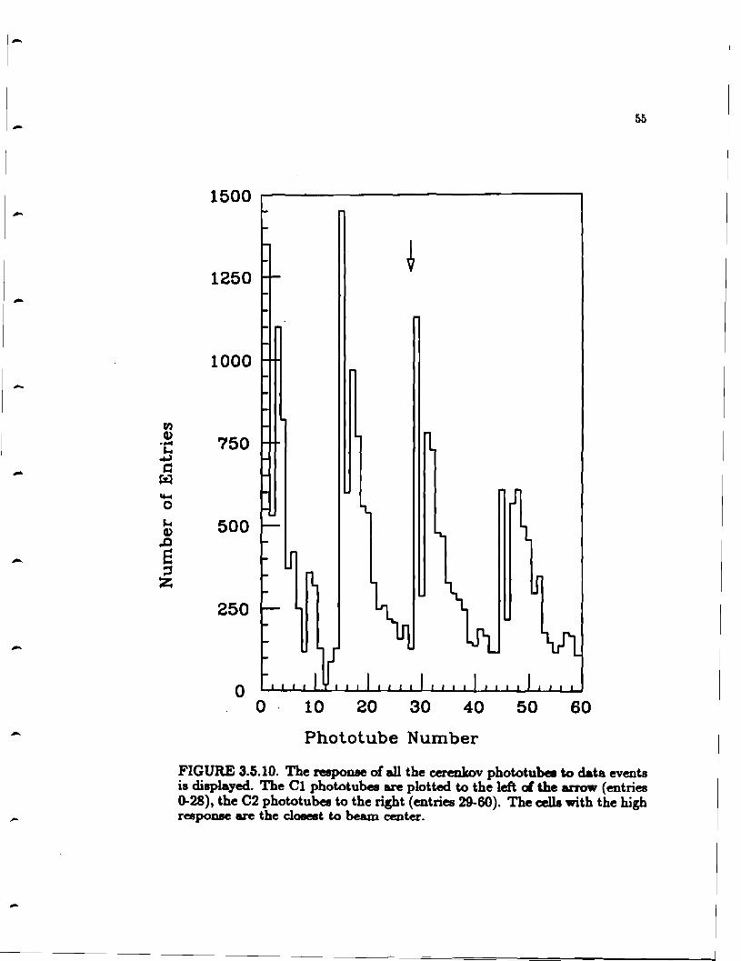
-
-
-
-
-
-
-
-
-
SS
1250
1000
750
500
250
0 0 . 10 20 30 40 50 60
Phololube Number
FIGURE 3.5.10. The reepome of all the cerenkov phototubee to data events is displayed. The Cl phototuhes are plotted to the left al. the arrow (entries 0-28), the C2 phototuhes to the right (entries 29-60). The cella with the high respome are the cloaest to beam center.

56
NUMBER OF PHOTOELECTRONS VERSUS RUN NUMBER
20 17.5 Cl
15 ~ 12.5 6 6 6 A 10 0 A~
z 7.5 6 a 6
5 MIRROR # 19 o 2.5 · I 6
0o.a 1.2 1.0 2.0 2.4 2.8 3.2 RUN NUMBER ( af03)
20 17.5 C2
15 ~12.5 A 10
z 7.5 MIRROR ti 17 a 5 ·• 5 6 2.5
0 0.8 1.2 1.0 2.0 2.4 2.8 3.2
RUN NUMBER ( 1103)
FIGURE 3.5.11. Gain curves for two cerenkov cells are displayed. The gain of a cell ia the final measure of its performance since it ia the "maximum average response of the cell to a single track".
...
--
-
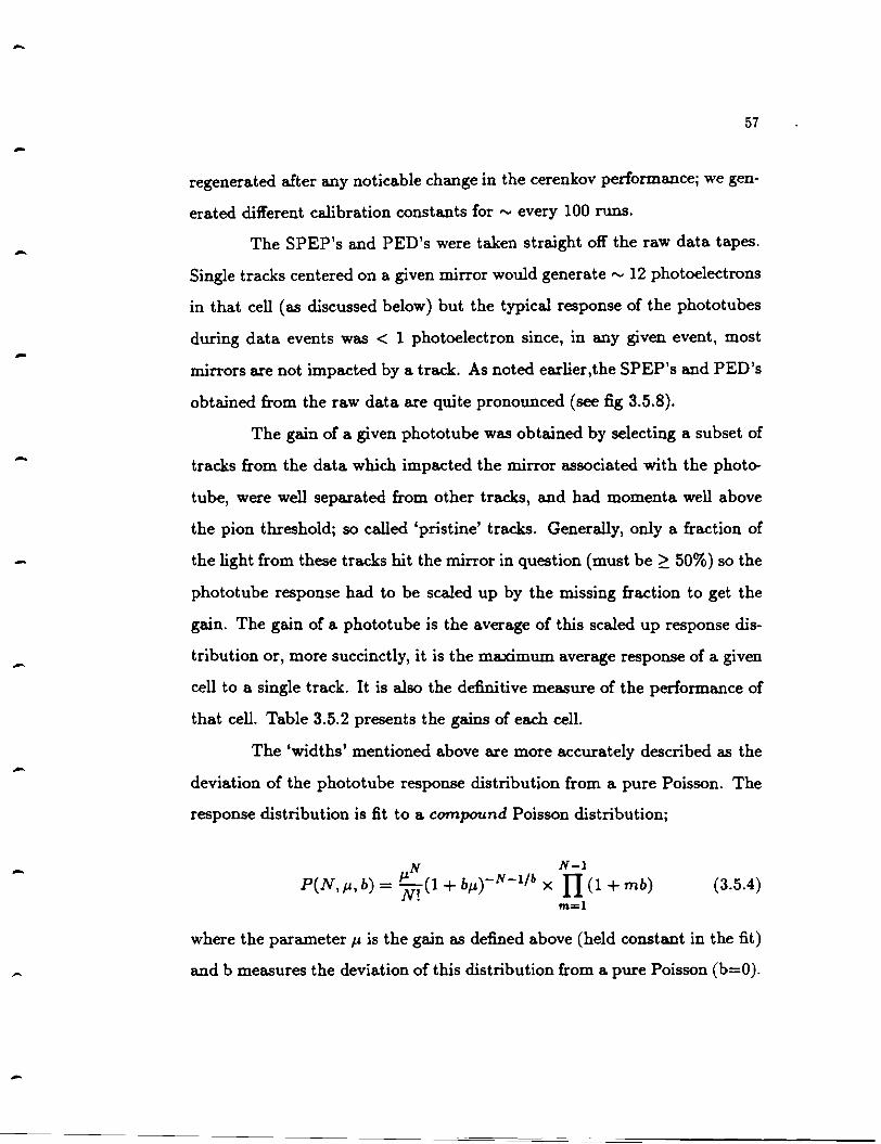
-
-
-
-
-
-
-
-
-
57
regenerated after any noticable change in the cerenkov performance; we gen
erated different calibration constants for - every 100 runs.
The SPEP's and PED's were taken straight oft' the raw data tapes.
Single tracks centered on a given mirror would generate - 12 photoelectrons
in that cell (as discussed below) but the typical response of the phototubes
during data events was < 1 photoelectron since, in any given event, most
mirrors are not impacted by a track. As noted earlier,the SPEP's and PED's
obtained from the raw data are quite pronounced (see fig 3.5.8).
The gain of a given phototube was obtained by selecting a subset of
tracks from the data which impacted the mirror associated with the photo
tube, were well separated from other tracks, and had momenta well above
the pion threshold; so called 'pristine' tracks. Generally, only a fraction of
the light from these tracks hit the mirror in question (must be ~ 50%) so the
phototube response had to be scaled up by the missing fraction to get the
gain. The gain of a phototube is the average of this scaled up response dis
tribution or, more succinctly, it is the maximum average response of a given
cell to a single track. It is also the definitive measure of the performance of
that cell. Table 3.5.2 presents the gains of each cell.
The 'widths' mentioned above are more accurately described as the
deviation of the phototube response distribution from a pure Poisson. The
response distribution is fit to a compound Poisson distribution;
N N-1
P(N, µ, b) = ';;, (1 + bµ)-N-l/b x IT (1 + mb) m=l
(3.5.4)
where the parameterµ is the gain as defined above (held constant in the fit)
and b measures the deviation of this distribution from a pure Poisson (b=O).

58
Although each incremental element of the photocathode emits photoelectrons
with a Poisson distribution, the integrated response of the photocathode is
described more accurately with the compound Poisson distribution because
of the variation of the photocathode conversion efficiency across the face of
the phototube. The b parameters were derived once and assumed to hold
constant throughout the run (in all cases, b<10%). With a well defined
model for the response of the phototube, we could compare the number of
photoelectrons obtained for a given track, NPH ( eqn 3.5.3), with the expected
number for each viable mass hypothesis and; thus, were able to derive the
probabilities for this track. The details of this process are given in section
5.2.2.
We began the process of aligning the Cerenkov mirrors with respect
to the drift chamber coordinate system by measuring the positions of the
mirrors relative to one another. A set of isolated, high momentum tracks
similiar to the set used to generate the gains was then selected. As we varied
the position of each central mirror within the mirror plane, the subset of
tracks that impacted the mirror at each new position was determined and
the frequency with which these tracks prompted a response in that mirror's
phototube was plotted. The x-y position of the mirror evoking the highest
response rate was chosen to be the "true" mirror position as measured in the
drift chamber coordinate system. The x-y offsets that were derived for the
central mirrors were then applied to the entire mirror set.
The final step in the calibration was to determine the threshold be
havior of the counters. We used isolated tracks of varied momentum and
observed the measured radiation in all the cells affected by this track as a
function of momentum, assuming these tracks were mostly pions. A fit (fig
-
-
-
-

59
Table 3.5.2: Cerenkov Cell Gains for Cl and C2
Mirror Cl C2 Mirror Cl C2
1 11.1 13.2 17 10.4 16.2
2 15.0 14.6 18 9.8 9.6
3 14.4 14.2 19 14.6 11.4
4 12.3 12.6 20 16.4 14.4
5 8.0 12.9 21 13.9 17.0
6 18.2 13.9 22 14.0 13.9
7 10.8 13.7 23 14.2 14.1
8 7.5 12.3 24 11.1 14.3
9 12.9 16.3 25 14.7 12.5
10 9.9 14.9 26 15.1 9.1
11 14.3 13.2 27 7.8 6.9
12 13.3 7.6 28 14.6 9.4
13 12.1 13.3 29 14.0
14 16.6 13.8 30 13.4
15 18.0 12.6 31 16.2
16 22.2 12.2 32 13.0
-
-

60
3.5.12) to the observed number of photoelectrons was performed over a mo
mentum range which was below the kaon radiation threshold, thus excluding
kaon or proton contamination. The fit near the pion threshold was of the
form 1-p~h/p2 • This behaviour as a function of momentum was included in
the reconstruction algorithm (see section 5.2.2).
3.6 The SLIC and Pair Plane
Many important charm decay channels require good identification of
either a 7r'o or a high momentum electron (Do-+ K-7r'+7r'o, Do-+ K-e+v).
The SLIC, Scintillator Lead Interleaved Counter, was used to identify and
provide the energies and positions of electrons, positrons, and photons. Two
photon combinations were then used to form 7r'0s. In addition to this, the
SLIC was an integral element of the triggers.
The SLIC is shown in figure 3.6.1. It has 60 layers, each composed
of .32cm of lead and 1.3cm of liquid scintillator. This is the equivalent of 20
radiation lengths (and 2 interaction lengths) of material. The scintillator was
isolated from the lead (which would poison it) and segmented by corrugated
aluminum panels with corrugations of 3.2cm in the central region of the
counter and 6.4cm in the less confused outer region. These panels were
layered perpendicular to the beam with the corrugations either horizontal (Y
view), or at ±20.5° to the vertical (U, V view respectively). The aluminum
panels were coated with tefton and since tefton has a lower index of refraction
than the scintillator, light emitted in the scintillator at < 20° to the tefton
surface was totally internally reflected. This scintillator light could then be
efficiently transported to the light collection apparatus.
The segments in the z direction in each of the three views were
collected into a single channel by a w'aveshifter bar (see fig 3.6.1). This
-
-
-
-

-
-
-
-
-
-
-
-
-
61
100 x C1 (P01 5.95±0.02GeV/c)
• Cz (Pu1 10.16±0.05GeV/c)
-~ 0 -.,, .ri+Ii-I~:tUi • -u -.,,
• r i--i ~
£L 50 I I/ z I
, ..... E I .,, I ,i • I ~
:I s a • I ., c • I ~ I /.
z , I ,~· z s
~•z--z-
0 :2 4 . 6 8 10 12 14 16 18 20 22 24 26 P(GeV/c)
FIGURE 3.5.12. The momentum threshold of both Cerenkov counters is displayed. The curves are generated with light emitted by pions only (the curves are cut off before the kaon light threshold is reached). The fraction of light measured well above threshold is < 1003 because some of the light emitted by the track misses the mirror being sampled.

... , ,, ' ....
~. 114• STEEL ',, REIWORCING BARS '
WAVEBAR-...c
PMT-...... ...,_y VIEW.
c 58 COlNrERS EACH SIDEJ
62
FIGURE 3.6.1. Schematic of the LeM:l/Liquid Scintillator Shower Counter (SLIC).
-
-
-
-
-
-
-
-
63
bar shifted the ultra-violet scintillator light into green light for which the
phototubes (2" RCA4902 in the central region/3" RCA4900 in the outer
region) were more efficient. The anode output of the phototubes was read
into LRS 2280 ADCs while _the dynode signal was fed into the trigger. The
U and V views had 109 channels each, read out at the top and bottom of
the counter respectively while the Y view had 116 channels with half read
out on the east side and half on the west side of the detector.
The same clean muons used to calibrate the drift chambers were used
to calibrate the SLIC. Pairs were also used to check the consistency of the
muon calibration, at least in the central counters accessible to them. Details
of the calibration are discussed elsewhere. 1221
The pair plane was a set of 19 counters lined up in x and placed
directly behind the last drift chamber assembly (D4), at beam height. These
absorption counters constituted 20 radiations lengths of material and were
followed by 10 radiation lengths of lead. The C-counter, discussed in section
2.3, was the central pair plane counter. The pair plane was to serve two
functions, to help filter pairs out before they reached and Hooded the SLIC,
and to measure the energy of the particles that it absorbed. As in the case
of the C-counter, the congestion in this region prevented us from making
reliable measurements of the energies of the absorbed particles.
3.7 The Hacirometer
Good neutral hadron detection would have given us access to some
otherwise inaccessible charm decay modes (e.g. modes with E- - n71'
(100%)). Unfortunately, the fractional energy resolution of the hadrometer
was 75% /VE which prohibited effective analysis. The default responsibility
of the hadrometer was as an element of the triggers for which it played an
64
important role. It was also used a.s a hadron veto for the SLIC and to
augment the muon identification.
The hadrometer was a multilayer steel and scintillator sandwich (fig
3.7.1) used to detect energy from hadron showers and from the passage of
muons. It wa.s comprised of an upstream and downstream module, separated
by a 5cm airgap, and with 18 layers in each module. The layers contained
2.5cm of steel and lcm of scintillator each. The hadrometer provided 2 views,
X and Y, which were alternated with each layer, and read out on the top (X
view) and on the sides (Y view). The 38 Y and 33 X channels were formed
by summing, in the z direction, the nine channels belonging to each view in
each module. These signals were transported by lucite lightguides to 5" EMI
9791KB phototubes and readout by LRS 2280 ADCs.
The hadrometer was calibrated cell by cell using the same set of
calibration muons a.s the SLIC. This wa.s an important task because the
dynode outputs from the hadrometer channels were used in the Et trigger.
Details of this calibration process are found elsewhere1221 •
3.8 The Muon Wall
The main function of the muon wall was to detect high energy muon
pairs for the J /,,P analysis. It was also used in coincidence with the front
muon wall to trigger the calibration muons used in the drift chambers, the
SLIC, and the hadrometer.
The wall of 46cm and 61cm scintillators used to detect the muons
wa.s separated from the hadrometer by - lOOcm of steel. Low energy muons
and effectively all hadrons were absorbed before reaching the wall. The scin
tillator light wa.s transported by lightguides to 5" EMI 9791KB phototubes,
the outputs were discriminated and latched, and the discriminator output
-
-
-
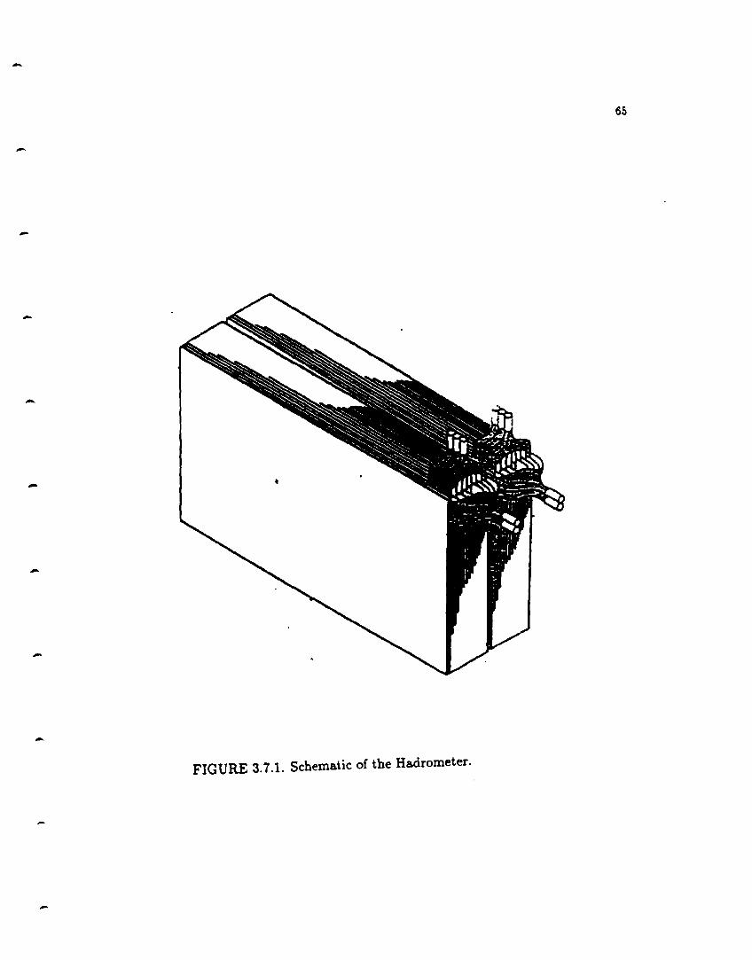
-65
-
-
-
-
-
-
-FIGURE 3.7.1. Schematic of the Hadrometer.
-

66
used to stop a TDC from which we could obtain a measure of the y posi
tion of the muon. The efficiencies of the counters and the reference values
for the TDCs were derived by setting a double paddle counter behind each
muon counter at 3 different positions and requiring a triple coincidence of
this muon counter with the paddle counters.
-
-
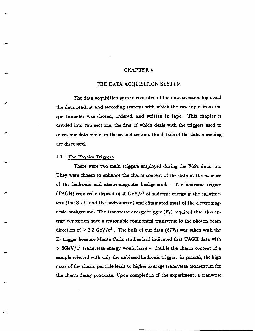
-
-
-
-
-
-
-
-
-
-
CHAPTER4
THE DATA ACQUISITION SYSTEM
The data acquisition system consisted of the data selection logic and
the data readout and recording systems with which the raw input from the
spectrometer was chosen, ordered, and written to tape. This chapter is
divided into two sections, the first of which deals with the triggers used to
select our data while, in the second section, the details of the data recording
are discussed.
4.1 The Physics Triggers
There were two main triggers employed during the E691 data run.
They were chosen to enhance the charm content of the data at the expense
of the hadronic and electromagnetic backgrounds. The hadronic trigger
(TAGH) required a deposit of 40 GeV /c2 of hadronic energy in the calorime
ters (the SLIC and the hadrometer) and eliminated most of the electromag
netic background. The transverse energy trigger (Ei) required that this en
ergy deposition have a reasonable component transverse to the photon beam
direction of~ 2.2 GeV /c2 • The bulk of our data (87%) was ta.ken with the
Ei trigger because Monte Carlo studies had indicated that TAGH data with
> 2Ge V / c2 transverse energy would have ,..,, double the charm content of a
sample selected with only the unbiased hadronic trigger. In general, the high
mass of the charm particle leads to higher average transverse momentum for
the charm decay products. Upon completion of the experiment, a tranverse

68
energy cut of 2.2 GeV /c2 was applied to the TAGH data sample. The re
sultant sample contained 80% of the charm found in the original sample yet
contained only 1/3 as many events; an enhancement factor of> 2.5.
The TAGH trigger required the coincidence of an interaction (de
tected by the B-counter) and a 40 GeV /c2 deposition in the calorimeters. No
TAG was required. The Et trigger, besides requiring> 2.2 GeV /c2 transverse
energy, needed either a TAGH with a good TAG or a TAGH with a mini
mum energy deposition of 70 Ge V / c2 in the calorimeters (to allow for poor
tagging of very high energy photons) plus some minimal response from the
first Cerenkov counter (Cl). This last coincidence was necessary because
the PCENTER beam would periodically flood our experimental hall with
muons that, combined with a typical hadronic interaction, would imitate an
Et event beautifully.
The Et and TAGH trigger schematic is shown in figure 4.1.l. All the
dynode signals from the SLIC and the hadrometer were input to LRS 628
NIM modules at Level 1. The dynodes in each individual module were from
counters approximately equidistant from the SLIC or hadrometer detector
center. At this point, the SLIC output was attenuated by 12dB, as indicated
by the relative calibration of the two calorimeters, and summed with the
hadrometer output to form the hadronic energy. The relative transverse
energies of each module were formed at Level 2 by attenuating the Level 1
outputs with the appropriate resistors. They were summed at Level 4 to get
Et where, again, the SLIC response had to be attenuated by 12dB. At each
level, the output was sampled and monitored to ensure the performance of
the trigger. The Ee signal was then fed into a charge discriminator module
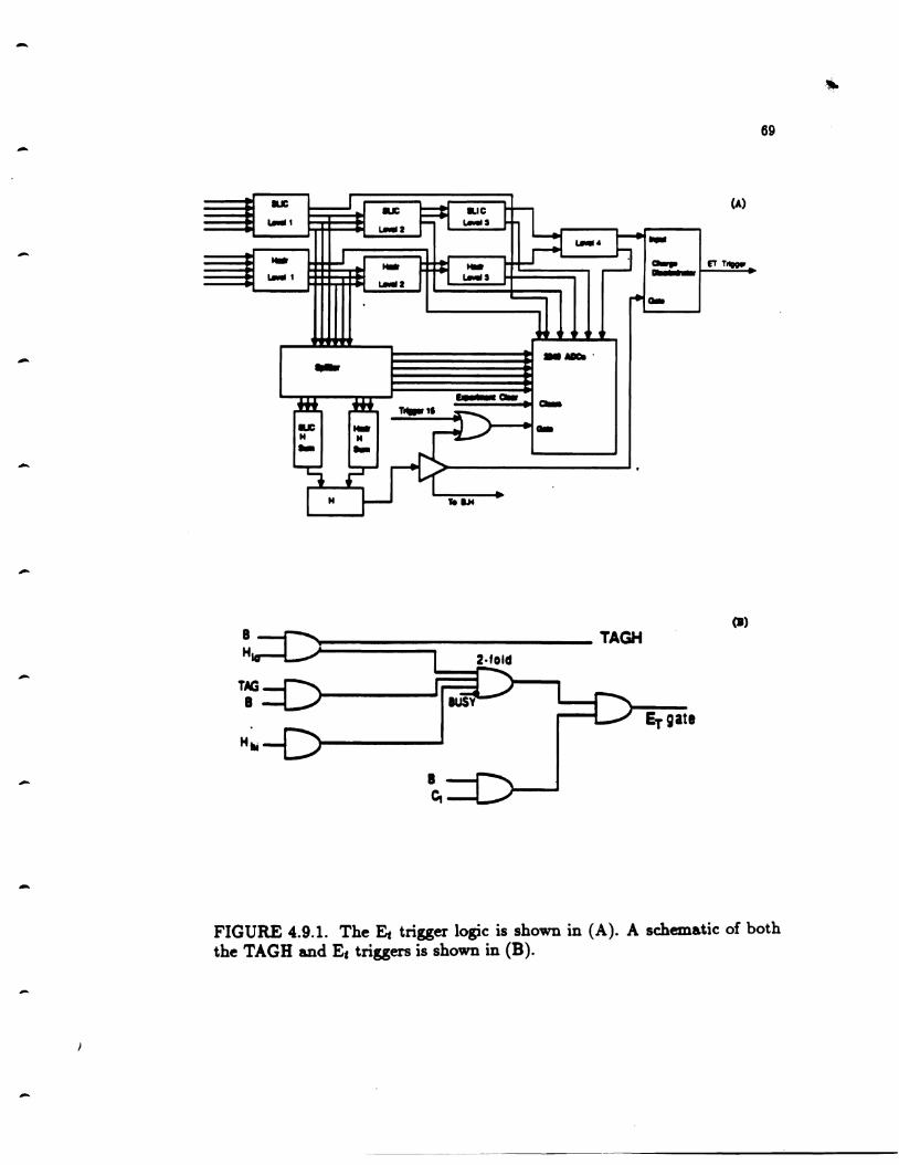
-
-
-
-
-
-
-
TAG 8
Hlli
a.a:: lallll ,
.. ...... ,
69
(A) .. a.,. ETT ..... ...... a..
(B)
Er gate
FIGURE 4.9.1. The Et trigger logic is shown in (A). A schematic of both the TAGH and Ee triggers is shown in (B).
70
with which we applied the Ee cut on our data. The discriminator unit was
calibrated along with the calorimeters and we obtained the relation· '
Ee = .36 + .4xN where N=discriminator setting
=4.5 for Ee >2.2GeV /c2 •
From figure 4.1.2, it appears that choosing Ee > 2.2GeV /c2 was
rather conservative. However, the experimental dead.time rose with Ee and,
since maximizing the charm written per second was our goal (and not maxi
mizing the charm written per tape), the Ee cut was set at a lower value than
this simple curve indicated. A discussion of the dimuon trigger and the other
trigger types used in E691 as well as details on the charge discriminator unit
can be found elsewhere1391 •
4.2 The Data Recording
The data recording system was responsible for collecting, organizing,
and recording onto tape the response of our spectrometer to the photon
interaction. For most of our data (93% ), the calibration triggers, the Ee
trigger, and the dimuon trigger were fed into a logical OR which indicated
when an acceptable trigger had been generated (for the other 7% of our
data, the TAGH trigger was added to this OR). If this OR was within the
beamgate generated by the B-counter, and if the CAMAC was ready to
accept new data (the computer wasn't reading CAMAC out to memory or
another trigger's response wasn't being digitized) this OR would prompt a
BEAM STROBE which began the gates for the ADCs, sent the TDC stops,
and strobed the Latches. A BUSY indicator which rejected all new triggers
was also set by the computer at this time. If the computer wasn't writing
events on tape, this strobe would initiate a computer interrupt so that this
event could be transferred from CAMAC to the computer's memory. Once
-

-
2.5 5.0 7.5 I 0.0 6-------------------------....-------------..-...6
-~ 4 E • (,)
c a &. 2 c
LI.I
4
2
00 __ __._._ ........ ..._ ..... _2 .......... ..-._...~3--......... ..-4 ....... _,_......_.~5o
Er (GeV)
71
FIGURE 4.1.2. Charm enhancement as a function of transverse energy is displayed. The lower scale gives the transverse energy in GeV /c2 while the upper scale is the hardware value at which the charge discriminator was set.

72
the event was safely in the memory, the BUSY was dropped and a CLEAR
was sent to the CAMAC.modules to ready them for new data.
The fraction of the time that this system was unresponsive to new
data is referred to as the deadtime, whether the computer is writing tape
or reading out CAMAC, or another event is being digitized. For E691, we
had a measured deadtime of ,..,, 30% while ta.king data at approximately
100 events/sec. The data acquisition hardware (fig 4.2.1) consisted of a
PDP-11/55 computer with fast bipolar memory and two Jorway 411 CA
MAC branch drivers for the two CAMAC branches employed by E691. The
tapedrive was an STC 1921. It is worth noting that positioning the tapedrive
between the CPU and the branch drivers allowed us to write tape while the
CAMAC digitized data which almost doubled our DA rates. This would
not have been possible if the positions of the tape drive and the CAMAC
were reversed because the device closest to the CPU had priority for data
transfers.
-
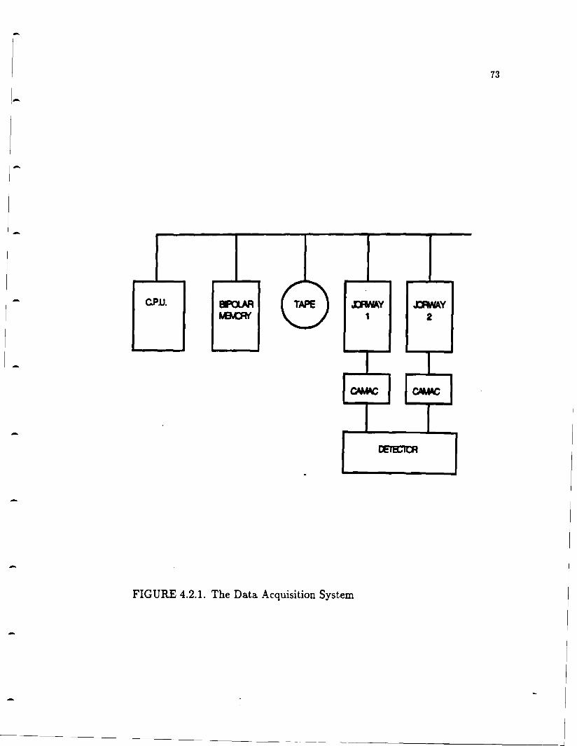
73
C.P.U. BFClAR ~ TAPE ) .rswAY DWAY M:M:Rr' \... 1 2 -
QtlMC C¥MC
CEIS::I~
-
FIGURE 4.2.1. The Data Acquisition System

CHAPTER 5
THE RECONSTRUCTION PROGRAM
The raw data events written at TPL contained many thousands of
strictly ordered, scrupulously monitored drift chamber drift times SMD hits ' '
phototube pulse heights, and set latch bits. These had to be sensibly con
verted to particle types, positions, and momenta. A computer program,
therefore, had to be written which would read in this raw data, interpret it,
and output the above information.
The E691 data reconstruction computer program was divided into
two steps called PASSl and PASS2. PASSI handled pattern recognition
(track finding) and the momentum determination, while PASS2 used PASSl
output to reconstruct the raw tagging, SLIC, and Cerenkov information and
to find the candidate vertices in the data. On average, PASSl used .7 Cy
ber 175 seconds of CPU time per event and PASS2 used .25 seconds per
event. Given these reconstruction rates and the size of the Fermilab Cyber
Computer system, complete reconstruction of the 108 data events written
at TPL would have taken ,..,, 3 years. We were fortunate, however, to have
access to a microprocessor farm (the Advanced Computer Program (ACP)),
which, since it was dedicated to E691, reconstructed our data ,..,, 10 times
faster than the Cyber system. Due to this dramatic increase, the data set
was reconstructed more than a year earlier than had been projected.
-
-
-

-
-
-
75
5.1 PASSl
The PA5Sl program had two main internal routines; 51234 and
5E5TR. The 51234 routine was responsible for searching the 5MD for tracks
originating in the target while the 5E5TR routine was used to find tracks
originating downstream of the 5MD (e.g. A0 , K~ decay products). 51234
ran first and it began by finding the tracks in the region upstream of the
first magnet (see figure 3.0.1). The track finding started in the SMD and
not the (less congested) drift chambers because of (a.) the superior tracking
efficiency of this detector, (b) the excellent redundancy ( 3 planes for each of
the XYV views in the 5MD, 2 planes for each of the XUV(X') views in Dl)
of the SMD /D 1 region, ( c) the fact that we start the tracking in the region
of best resolution, and (d) the high reconstruction rates obtained with this
method.
Tracks with three hits in any 2 of the 3 5MD views were considered
first. The track segment defined by these 2 views was projected into the
third view and tracks with 3, 2, or 1 hits in that view were selected. Tracks
with hit patterns of 3-2-2, 3-2-1, and 2-2-2 respectively were then picked up
using Dl to help with the views with less than 3 hits. Having established
the SMD/Dl track candidates, 51234 would project them into D3 in the Y
view (D3 was less congested than D2) and link these tracks to XUV triplets
in that drift chamber. Linking was initiated in the Y view because the fields
bent the particles appreciably only in the X direction. The X position of a
matched triplet established the horizontal bend of the track and thus fully
constrained it. Using a single bendpoint approximation for the magnetic
fields, we then swam the track through the entire detector and the drift
chamber triplets associated with this track were determined. S1234 would

76
then perform a momentum fit on this track candidate using these triplets,
the SMD information, and the full field map of the magnets. Finally, the
S1234 routine applied the track quality cuts to this set of tracks; dropping
tracks with too few SMD hits, with a bad x2 from the momentum fit, and
tracks that shared too many hits with a stronger track. The overall tracking
efficiency obtained was > 90% for high momentum tracks. This routine took
.5 seconds of CPU time on average and one second on average for charm
events, which were higher multiplicity events.
The SESTR routine was called at this point to search for tracks
originating outside the SMD. It ran quite efficiently, needing only .2 sec/event
of CPU time, because hits assigned to SMD tracks by 51234 weren't reused
in this tracking package.
5.2 PASS2
5.2.1 The SLIC Reconstruction Program
The SLIC reconstruction was a complex multi-step process. First,
the counter outputs were converted to physical energies using gain curves
obtained during calibration. Adjacent counters in each view whose energies .
were above a particular threshold were then grouped into 'cells'. These cells
were, in turn, split into 'sectors' which were defined as any set of counters
within this cell whose central counter energy was a local maximum. A list
of candidate sectors was constructed for each cell.
b . ed . . fit 13111 These candidate sectors were su Ject to a stepwise regression
in order to determine the final set of sectors for this cell and to sensibly dis
tribute the cell energy among them. The fit also generated the sector energy
errors which were determined by the significance of the energy deposition in
-
-
-

-
-
77
the sector as well as the nature of the deposition (hadronic or electromag
netic). A list of candidate particles was then created for the event. If well
defined energy depositions in the V and Y view could predict the position
and magnitude of a U deposition, the YUV triplet was considered a candi
date. The set of candidates was subjected to another stepwise regression fit
in order to determine the SLIC particle list, the particle energies, and the
energy errors.
These particles were then checked to make sure that the showers as
signed to them were electromagnetic in character. The probability tha.t the
energy deposition associated with a given SLIC particle was electromagnetic
was estimated by comparing the transverse energy distribution associated
with ea.ch particle to electromagnetic shower shapes created by Monte Carlo
simulations and stored in the reconstruction code. This check was impor
tant because large hadronic showers would often generate smaller 'satellite'
showers that could effectively imitate the energy depositions of genuine SLIC
particles. Using this comparison, we could filter these 'satellite' showers out.
In additio~, the probability derived above was included in the derivation of
the overall probabilities assigned to the SLIC particles.
The major problems encountered in this reconstruction had to do
with overlapping energy depositions in the central region and the 'hadronic
satellite' shower problem mentioned a.hove. The hadronic satellite showers
were handled not only by comparing measured and predicted shower shapes
as described above, but also by comparing the location of the SLIC energy
deposit with the energy deposit in the ha.drometer from this track, and by
throwing out small candidate sectors which were close to large energy de
positions. The fractional energy resolution obtained for the SLIC was ~.
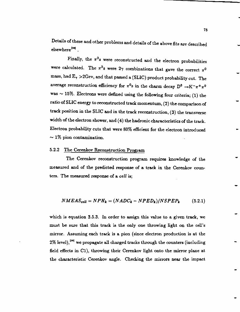
78
Details of these and other problems and details of the above fits are described
elsewhere 1381 •
Finally, the 7r0s were reconstructed and the electron probabilities
were calculated. The 7r0s were 2")' combinations that gave the correct 7ro
mass, had E.,, >2Gev, and that passed a (SLIC) product probability cut. The
average reconstruction efficiency for 7r0s in the charm decay no ~K-7r+7ro
was - 15%. Electrons were defined using the following four criteria; {1) the
ratio of SLIC energy to reconstructed track momentum, (2) the comparison of
track position in the SLIC and in the track reconstruction, (3) the transverse
width of the electron shower, and ( 4) the hadronic characteristics of the track.
Electron probability cuts that were 80% efficient for the electron introduced
- 1 % pion contamination.
5.2.2 The Cerenkov Reconstruction Program
The Cerenkov reconstruction program requires knowledge of the
measured and of the predicted response of a track in the Cerenkov coun
ters. The measured response of a cell is;
NMEAScell = NPHt = (NADCt - NPEDt)/NSPEPt {5.2.1)
which is equation 3.5.3. In order to assign this value to a given track, we
must be sure that this track is the only one throwing light on the cell's
mirror. Assuming each track is a pion (since electron production is at the
2% level), 1391 we propagate all charged tracks through the counters (including
field effects in Cl), throwing their Cerenkov light onto the mirror plane at
the characteristic Cerenkov angle. Checking the mirrors near the impact

-
-
-
-
-
79
position in the mirror plane of a specific track, we can identify that set of
M cells (M$4) into which only this track throws light; denoting this set of
mirrors as C(M). The measured response of these cells can then be uniquely
assigned to this track;
Ntracl:,cell = N;,l: =NM EAS1;;; k E C(M).
The predicted response of these cells is calculated as follows. Con
sider only the set of cells, C(M), into which this track throws Cerenkov light.
The track throws only a fraction of its light onto a given cell's mirror; call it
Fgeo. In addition, the phototube response to a track near threshold is scaled
down by the fraction (see section 3.5.3);
(5.2.2)
where the threshold momentum, P,1&, is derived in the calibration. Ffeo and
Fmom a.re derived for each track, for each Cerenkov cell, and for all viable
mass hypotheses (from the set; [e-, µ, 7r,K, p] see section 3.5.1). Multiplying
the gain (the maximum average response of a cell to a single track) by these
fractions, we get the general expression for the predicted response of a cell
to a given track with a given mass;
N PREDmau tracl: cell= Iii 1· 1;; = F,~,~oL x Ft1·0 m x GAIN1;;. , ' '' , ,~ , (5.2.3)
The task now at hand is to generate probabilities for each track and
each mass hypothesis, by comparing the predicted and measured responses
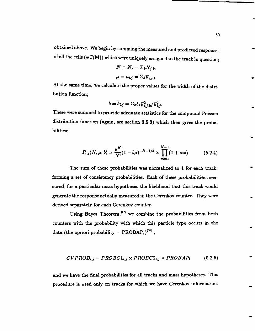
80
obtained above. We begin by summing the measured and predicted responses
of all the cells ( EC(M)) which were uniquely assigned to the track in question;
N = N; = "E1;N;,1;,
µ = µi,j = "E1;µi,j,I:
At the same time, we calculate the proper values for the width of the distri
bution function;
These were summed to provide adequate statistics for the compound Poisson
distribution function (again, see section 3.5.3) which then gives the proba
bilities;
N N-1
Pi,;(N, µ, b) = ~! (1 - bµrN-l/I> x II (1 + mb) (5.2.4) m=l
The sum of these probabilities was normalized to 1 for each track,
forming a set of consistency probabilities. Each of these probabilities mea
sured, for a particular mass hypothesis, the likelihood that this track would
generate the response actually measured in the Cerenkov counter. They were
derived separately for each Cerenkov counter.
Using Bayes Theorem, 13TJ we combine the probabilities from both
counters with the probability with which this particle type occurs in the
data (the apriori probability= PROBAPi}'311 ;
CV PROB··= PROBCl· · x PROBC2· · x PROBAP.· 1,J 11J l,J I (5.2.5)
and we have the final probabilities for all tracks and mass hypotheses. This
procedure is used only on tracks for which we have Cerenkov information.
-
-
-

-
-
-
-
81
Tracks with no unshared mirrors or tracks that don't traverse the Cerenkov
counters a.re simply assigned the apriori probabilities.
Figure 6.1.1 shows A0(fig 6.1.la,b) and K.,(fig 6.1.le,f) mass plots
before and after Cerenkov product probability cuts on their neutral decay
products. For both neutral particles, it is clear that the Cerenkov cut drops
the background by a factor of two without significantly affecting the signal.
5.2.3 The Vertexing Reconstruction
The vertexing reconstruction began with a global refit of all SMD
tracks using only SMD hits. Information from Dl was used only to assign
SMD hits to weak tracks, as this information didn't improve the vertexing.
The procedure began by finding a 2 track vertex with x2 per degree of free
dom( dof) < 3. Tracks are then added to this vertex, keeping only those for
which the overall x2 /dof remained under 3. The rejected tracks formed a
new track set which was handled in the same manner as the initial track
set. This procedure was followed until all tracks that could be assigned to a
vertex were so assigned.
In practice, a similiar vertex set had to be reconstructed for every
candidate secondary vertex. In the analysis, one first chooses the track com
bination of interest, calculates its vertex {the secondary vertex) and x2 /dof,
and then excludes these tracks from the main vertex track set. The vertex
package (not including the global refit) is then run on the track subset to
generate the candidate main vertices. Each secondary vertex selected in this
manner is independent of the candidate main vertex set and, thus, a reliable
measure of the separation of the main and secondary vertices can be made.
Errors on the vertices, including contributions from multiple scatter
ing as well as from the vertex fit itself, are typically;

82
50 Uz ~ 13 + p(_Gev)µm (5.2.6)
3.3 UtJz/tl• ~ 0.1 + p(_Gev) mrad. (5.2.7)
Figure 5.2.1 shows an exceptional event with two vertices associated with
charm particle decays. The error ellipses shown represent - lu errors. -
-
-
-
-
-

-
-
-
-
-
0
-0.4
-e u -o.e -• -0 .~ -1.2 "O ~
0 0 u I
N
-1.6
-2.0
-2.4
-0.15 -0.14 -0.13-0.12 -0.11 -0.1-0.09-0.08-0.07 X- Coordinate (cm)
83
FIGURE 5.2.1. Charm event with two charm decays and main vertex reconstructed.

CHAPTER 6
THE ANALYSIS
A search through the full 108 event sample was made for decays
of the four A! states; A7r, A7r7r7r, pKo, and pKo7r7r. The charge conju
gates states are included for each of these decays. Theoretical predictions
for the two-body modes (A7r,pKo) exist which makes these modes particu-
1 I . t t• 111 •13
·u1 Th ul . b d d d (A - ) ar y m eres mg. e m ti- o y ecay mo es 7r7r7r ,pKo7r7r also
engender interest because the branching fractions in these modes are not
well known experimentally. The analysis of these modes involved first select
ing the neutral particle data samples and then determining the appropriate
event selection criteria separately for each mode. The vertex analysis of the
two-body modes was especially challenging since a standard charm decay
vertex could not be defined. In this chapter, the neutral particle strips and
the charm decay mode substrips are discussed in detail as a prelude to the
discussion of the final analysis cuts and the physics results in chapter 7.
6.1 The Neutral Pa.rticle Cuts
The initial step in the analysis was to select the neutral particle data
samples (A0 - p7r, Ko - Ka - 7r7r). Data samples are chosen, in general,
using physically sensible event selection criteria. With the neutral particle
decay samples, the track quality and Cerenkov behavior of the neutral decay
products had to meet certain criteria as did the invariant mass and decay
vertex formed from these two tracks. These criteria are presented below.
The selection criteria, or 'cuts', chosen for the lambda (A0) data sample
-
-
-
-

-
-
-
-
85
preserved about 3/4 of the reconstructed A0 s (reconstruction efficiency"' .5)
while reducing the background by almost a factor of 10. The cuts chosen
for the K,, sample preserved 3/4 of the reconstructed signal (reconstruction
efficiency ,..., .6) while reducing the background by a factor of 10 (see figure
6.1.1).
The A0 cuts are outlined in Table 6.1.1 and described as follows.
First, tracks detected in the SMDs ('SESTR' tracks) were excluded. The
neutrals were thus formed using only 'ESTR' tracks; tracks detected only in
the drift chamber system. This dramatically reduced the number of track
combinations used to form A 0 candidates. The remaining tracks were then
subjected to a general set of track quality cuts (which were applied to all
tracks used in all the analyses, see Table 6.1.lA). The momentum fit per
formed on this track could have a x2 per degree of freedom (x2 /DoF) of
5 or less, the momentum of the track had to be less than 250 Ge V / c2. as
dictated by the electron beam energy, and all tracks had to penetrate at
least the first magnet. This last cut was enforced by limiting the 'category'
of the track (JCAT). To illustrate how track categories were determined,
consider a track which was detected in all four drift chamber stations. The
4 bits associated with these 4 drift chamber stations in the reconstruction
were all set 'on' and the track category was generated by summing the bits
for this track; JCAT=1+2+4+8=15. A fifth bit was set if the track quality
was poor. Restricting the track category between 3 and 15, as was standard
practice in the analysis discussed below, was equivalent to requiring a good
track that had been detected in at least the first two drift chamber stations,
and therefore, had a well defined momentum, since these chambers straddle
the first magnet.

86
200 160
U) 150 (A)
120 (BJ w er 100 80 I- 50 40 z w 0 0 ~
I. I 1.108 1.116 1.124 I .I 1.108 1.116 1.124 0 ~ 120 303t25 lCJ
100 310±22
"' 80 (0)
m 80 60 2 40 ::> 40 z 20
0 I. I 1.108 1.116 1.124 I. I 1.108 1.116 1.124
Mhrp) G1V 800
800
U) 600 tE) 600 (FJ
w 400 er 400
I- 200 200 z w 0 ~
0.48 0.5 0.52 0
0.48 0.5 0.52 0 ~600 CGl 600 (H)
"' 400 a:t400
~ 200 200 z
0 0 0.48 0.5 0.52 0.48 0.5 0.52
M brw) G1V
FIGURE 6.1.1. Plots (A-D) show the A0 signal prior to any neutral particle vertex cuts (A), after Cerenkov cut (B), after vertex position cut (C), and after DCA cut(D ). Plots (E-H) show the behavior of the K,,1aort signal with the same cuts. The plots were fit to a ga.ussian plus a linear background where the width and mass of the signal is allowed to float.
..
-
-
-
-
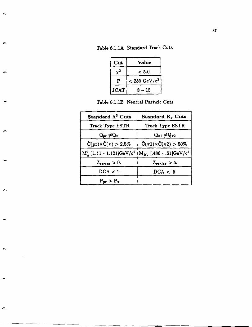
-87
- Table 6.1.lA Standard Track Cuts
Cut Value
x2 < 5.0
p < 250 GeV /c2
JCAT 3-15
- Table 6.1. lB Neutral Particle Cuts
Standard A° Cuts Standard K, Cuts
Track Type ESTR Track Type ESTR -QF~Qr Qrl ~Qr2
C(pr)xC('ll") > 2.53 C('11"1)xC(?r2) > 503
M~ [1.11 - 1.121]GeV /c2 Mx. [.486 - .5l]GeV /c2
- Zt1ertez > 0. Zt1erter > 5.
DCA < 1. DCA < .5
PF> Pr
-
-

88
For all A 0
candidates, the proton was chosen to be the track with
the highest momentum. In addition, the Cerenkov probability formed from
the product of the Cerenkov probabilities assigned to the A 0 decay products
(the proton and pion) had to be> 2.5%. Very low (Pproton < 5 GeV/c2 )
and very high momentum (P proton > 70 Ge V / c2 ) A 0s whose proton and pion
had been assigned the apriori Cerenkov probabilities were accepted with this
cut. Furthermore, the proton had to penetrate both magnets (JCAT ~ 5),
the distance of closest approach (DCA) of the proton and the pion tracks
had to be less than lcm, and the z position of the A0 decay (which is the z
position at which the DCA occurs) had to be greater than 0, where z=O is
the downstream end of the target. The z position cut eliminated background
from ESTR tracks that originate at the production vertex. Finally, the A 0
mass was constrained to be between 1.110 and 1.121 GeV /c2 . The set of A0
candidates defined by these cuts was the same for both the A 7r and A 7r7r7r
analyses.
The Kshort (K,) cuts are also outlined in Table 6.1.1. Again, the
decay products of the neutral particle had to pass the standard track quality
cuts while the product of their pion Cerenkov probabilities had to exceed ·
50%. Tracks detected in the SMD's were excluded from the analysis. The
K,, decay vertex had to be > 5cm from the end of the target and the DCA
of the two pions had to be < .5cm. Finally, the K,, mass was constrained to
be between .486 and .51 GeV /c2 .'3'1 This set of cuts remained unchanged
throughout the pK0 and pKo7r7r analyses. The subset of data events which
had combinations that passed the A 0 or K,, cuts were (separately) stripped
from the full data sample in order to make analysis of charm decay modes
containing these neutrals more convenient.
-
-

-
-
-
-
-
-
89
6.2 The Substrips
Although ea.ch of these neutral particle event subsets was only a
small fraction of the full set of 108 events, they were still very large (A0
strip: > 3 million events; J{,, strip: > 5 million events). Clearly, they had
to be reduced in size so the analyses planned for the charm decay modes
containing these neutrals could be done in a reasonable time. Therefore, a
'substrip' was performed on each neutral particle strip for each mode being
analyzed, with cuts that depended on that mode. The set of cuts used for
the substrips of ea.ch of the four At modes mentioned in the introduction
will now be discussed.
A computer program was written that could substrip the A0 strip for
both the A7r7r7r and the A7r decay modes. The list of cuts for these modes is
given in Table 6.2.1. The goal when substripping a data sample is to achieve
sufficient reduction in the size of the sample, while using the smallest number
of cuts possible, and without reducing the charm particle 'efficiency'. The
efficiency is the fraction of charm particle decays of a given mode that survive
all the cuts associated with that mode. It is determined by simulating the
response of the spectrometer to the charm particle decay using a Monte Carlo .
computer program (see section 6.4). These simulated raw data events are
then run through the reconstruction and analysis programs just like true raw
data events to estimate the effect of the chosen cuts on the charm signal in
question.
Cuts that don't affect the efficiency are, naturally, the first cuts we
apply to any substrip. For the A7r mode, the A0 strip was reduced from 3
million to .5 million events by requiring that the event have at least one A7r
combination with a mass between 2 and 2.5 GeV /c2 , and by requiring that

90
Table 6.2.lA Substrip Cuts: A11"11"11"
A11"11"11" Substrip A11"11"11" Analysis Strip E
Typerrr SESTR Typerrr SESTR .16 -Qr1 + Qr2+ Qr3 =QprA Qr1 + Qr2+Qr3 =QprA .145
MAt [2 - 2.5]GeV /c2 MAt [2 - 2.5]GeV /c2 .145
C3r > .25 .13
1 JCAT 3 Traclc Only .115
X~ec < 10 .078
DIP< 150µ .065
SDZ >4 .035 -RAT< 1 .019
Table 6.2. lB Substrip Cuts: pKo11"11"
pKo11"11" Substrip pKo11"11" Analysis Strip E
Type,rr SESTR Type,,rr SESTR .21
Qr1 = -Qr2 Qr1 = -Qr2 .19
MAt (2 - 2.5]GeV /c2 MAt (2 - 2.5]GeV /c2 .19
CprXCr1XCr2>10% Cpr x Cr1 x Cr2 > 20% .09
1 JCAT 3 Traclc Only .08
X~ec < 10 .05 -DIP< 150µ .04~
SDZ >4 .026
RAT <2 .02 -
-
-

91
-Table 6.2.lC Substrip Cuts: pKo
pKo Substrip pKo Analysis Strip f
Type"" SESTR Typepr SESTR .24
MAt [2 - 2.5]GeV /c2 MAt [2.1 - 2.5]GeV /c2 .24
Cpr > 20% c"" > 30% .14
- JCATpr ~ 5 .14
ITP,,,. > 0 .075
Table 6.2.lD Substrip Cuts: A7r
A7r Substrip A7r Analysis Strip f
Typey SESTR Typey SESTR .20
- Qr =QprA QT =QprA .20
MAt [2 - 2.5]GeV /c2 MAt [2. - 2.4]GeV /c2 .20
Cr> 70% .19
lcoscm(6)T I< .7 .14 -ITPr > 0 .075
-
-
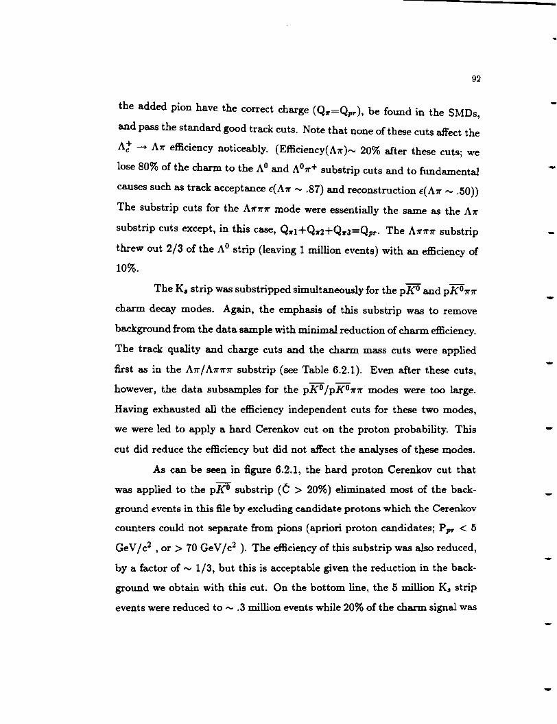
92
the added pion have the correct charge (Qr=Qpr ), be found in the SMDs,
and pass the standard good track cuts. Note that none of these cuts affect the
A! - A.Tr efficiency noticeably. (Efficiency(A.7r)"' 203 after these cuts; we
lose 80% of the charm to the A 0 and A 07r+ substrip cuts and to fundamental
causes such as track acceptance e(A.7r,..,, .87) and reconstruction e(A.7r,..,, .50))
The substrip cuts for the A.7r7r7r mode were essentially the same as the A.Tr
substrip cuts except, in this case, Qr1 +Qr2+Qra=Qpr· The A.7r7r7r substrip
threw out 2/3 of the A 0 strip (leaving 1 million events) with an efficiency of
10%.
The K. strip was substripped simultaneously for the pKo and pK07r7r
charm decay modes. Again, the emphasis of this substrip was to remove
background from the data sample with minimal reduction of charm efficiency.
The track quality and charge cuts and the charm mass cuts were applied
first as in the A.7r/A.7r7r7r substrip (see Table 6.2.1). Even after these cuts,
however, the data subsamples for the pK0 /pK07r7r modes were too large.
Having exhausted all the efficiency independent cuts for these two modes,
we were led to apply a hard Cerenkov cut on the proton probability. This
cut did reduce the efficiency but did not affect the analyses of these modes.
As can be seen in figure 6.2.1, the hard proton Cerenkov cut that
was applied to the pK0 substrip ( C > 20%) eliminated most of the back
ground events in this file by excluding candidate protons which the Cerenkov
counters could not separate from pions ( apriori proton candidates; Ppr < 5
Ge V / c2 , or > 70 Ge V / c2 ). The efficiency of this substrip was also reduced,
by a factor of,..,, 1/3, but this is acceptable given the reduction in the back
ground we obtain with this cut. On the bottom line, the 5 million K,, strip
events were reduced to ,..,, .3 million events while 20% of the charm signal was
-
-
-

-
-
-
-
-
-
93
preserved in the pK0 substrip. The pK011"1r mode was handled in like manner
except, in this case, a product Cerenkov cut was applied, with C,,rr > 10%.
This cut had essentially the same effect on the proton as the Cerenkov cut
discussed above and, in addition, low Cerenkov probability pions were re
jected as candidate charm decay tracks. The substrip for the pK0 7r7r mode.
reduced the K,, data sample by a factor of 5 with an efficiency of 11 %.
At this point, we had obtained substrip data files for each of the
4 modes of interest. These data files provided a convenient event sample,
containing the bulk of the reconstructable charm signal in each mode, from
which analysable data files could be stripped.
6.3 The Analysis Files
The final stripping programs were run on the substripped data at this
point to generate the (sub-substrip) data files for each mode on which data
analyses could be performed efficiently. All the cuts which were available for
use on these modes were applied at this last stripping level since we had to
reduce the hundreds of thousands of substrip events down to the level of a
few thousand events. These cuts are described below.
The vertexing cuts, which were used whenever a standard secondary
vertex could be defined (i.e. A7r7r7r, pKo7r7r decay modes), included the
DIP cut, the SDZ cut, the x;ec/DoF cut, and the RAT cut. The x;ec/DoF
cut variable was the x2 /DoF assigned to the secondary vertex by the least
squares vertex fit (the fit procedure is discussed in section 5.2.3). Recall that
the vertices generated by the reconstruction program had to have x2 /DoF
< 3. Similiar values for the x;ec/DoF of the secondary vertex were required
in the analysis.
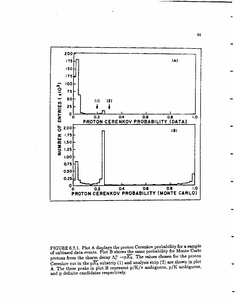
94
200-
175 I. - (A)
150
175.
- 100 ,_ ,,, 0 75 --JC . - 50 ._ (/) II.I 25 --
(I) (2) . ' a: 00 ...
z I .J"1 I I I
0.2 0.4 0.6 0.8 1.0 II.I PROTON CERENKOV PROBABILITY (DATA) I&. 0 2.00 (Bl a: 1.75 II.I m 1.50 s ::> 1.25 z
1.00
0.75
0.50
0.25
FIGURE 6.2.1. Plot A displays the proton Cerenkov probability for a sample of unbiased data events. Plot B shows the same probability for Monte Carlo protons from the charm decay A"t -+pKo. The values chosen for the proton Cerenkov cut in the p/(o substrip (1) and analysis strip (2) are shown in plot A. The three peaks in plot B represent p/K/rr ambiguous, p/K ambiguous, and p definite candidates respectively.
-
-
-
-
-
-
-
95
The DIP cut variable was derived in three steps. First, the charm
particle momentum was constructed from the charm particle decay products.
This vector was then forced to pass through the secondary vertex. Finally,
the distance of closest approach between the constrained charm momentum
vector and the main vertex was calculated (in the x-y plane perpendicular to
the beam and containing the main vertex). This is the Distance In the Plane
or DIP cut variable. This distance is zero for an ideal charm particle decay
since, in this case, the momentum vector of the charm particle connects the
main and secondary vertices.
The SDZ cut variable measured the significance of a given secondary
vertex with respect to the main vertex chosen in the analysis. It takes the
form,
SDZ=6z/u:i
where 6z is the separation between the main and secondary vertices and u :i is
the combination, in quadrature, of the errors in z assigned to the two vertices.
The secondary vertex and the candidate main vertex set were derived as
described in section 5.2.3. The main vertex chosen in the analysis was the
main vertex from this set associated with the smallest DIP.
The RAT cut variable for a given secondary vertex track was calcu
lated by finding the distance of closest approach between the main vertex
and this track (DCAm4 in) and between the secondary vertex and this same
track (DCA,,ec) and taking the ratio of DCAaec/DCAm4 in· This ratio was de
rived for all secondary vertex tracks and each such ratio was restricted to be
within the limit chosen for the particular charm decay mode being analysed.
A typical limit of RAT < 1 would select secondary vertex candidates whose
tracks were closer to their secondary vertex than to the chosen main vertex,

96
which is usually the case for tracks associated with a charm particle decay.
This cut was effective in ~lim.inating secondary vertex candidates where one
(or more) of the tracks associated with this vertex actually came from the
main vertex. We could not observe the A7r7r7r charm signal without this cut.
The cuts chosen to define the analysis data file for the A7r7r7r mode
are given in Table 6.2.lA. They were applied tightly (i.e. close to the op
timum value chosen in the final analysis) to achieve sufficient data sample
size reduction and this restricted our ability to study the cuts with this file.
Even with these tight cuts, however, the analysis data file was large; > 30K
events with an efficiency of"' 2%.
The analysis data file for the pKo7r7r decay mode is defined with a
set of vertex cuts sim.iliar to those used for the A7r7r7r mode as can be seen
in Table 6.2.lB. The Cerenkov product probability cut, Cp..,,., is tightened
as well. The combined effect of the vertex and Cerenkov cuts reduced this
data file to a reasonable size; < lOK events with an efficiency of "' 2%.
The substrip data sample for the A7r mode was not significantly
smaller than the A7r7r7r sample. Therefore, as in the last case, all the avail
able cuts had to be applied and applied tightly. These cuts were, however,
substantially different from the previous set of cuts because, as mentioned in
the introduction, we were not able to form a standard secondary vertex with
the decay products of this mode. The charm decay modes of this type, with
one neutral particle and one SESTR track, form a sub-class of modes; the
two-body modes. The basic analysis discussed below is the same for both
the pKo and A7r decay modes.
The initial thrust of the two-body analysis was to determine the
set of cuts that made the best use of the information available in these

-
-
-
-
-
-
-
97
modes. We have three tracks with well defined momentum (ESTR track
momenta errors are comparable to SESTR track momenta errors since the
momenta is determined largely by the drift chamber tracking (see section
3.3)) one of which, the SESTR track, has a well defined position. To begin
the analysis, we calculate the vector distance from the SESTR track to a
given main vertex candidate in the plane perpendicular to the beam direction
and containing the candidate vertex; call this DMISS (see figure 6.3.1).
We then break DMISS into components, one of which is contained in the
plane defined by the decay products of the charm particle. The remaining
component is approximately equal to the distance of closest approach of
the main vertex candidate and the charm decay plane (see below). These
distances are henceforth labeled In The decay Plane (ITP) and Out of The
decay Plane (OTP) distances respectively. The main vertex chosen in this
analysis is the candidate vertex associated with the smallest OTP distance.
The procedure used to find these values is as follows (figure 6.3.1 ).
We define a unit vector normal to the charm decay plane by taking the cross
product of the charm decay products; the SESTR track momentum with the
momentum of the neutral. This unit vector is approximately parallel to the
laboratory X-Y plane. Rotating the laboratory X axis counterclockwise1401
into this unit vector, we can define a new coordinate system with the unit
vectors xi and !ii. Expressing D MISS in this new coordinate system, we
see that DM ISS. xi is the Out of The decay Plane distance (OTP) and
DM ISS •!ii is the In The decay Plane distance (ITP).
We can also investigate the behavior of the secondary vertex for these
decays. Having chosen the main vertex as described above, we can pin the
charm momentum vector to this vertex and calculate the distance of closest
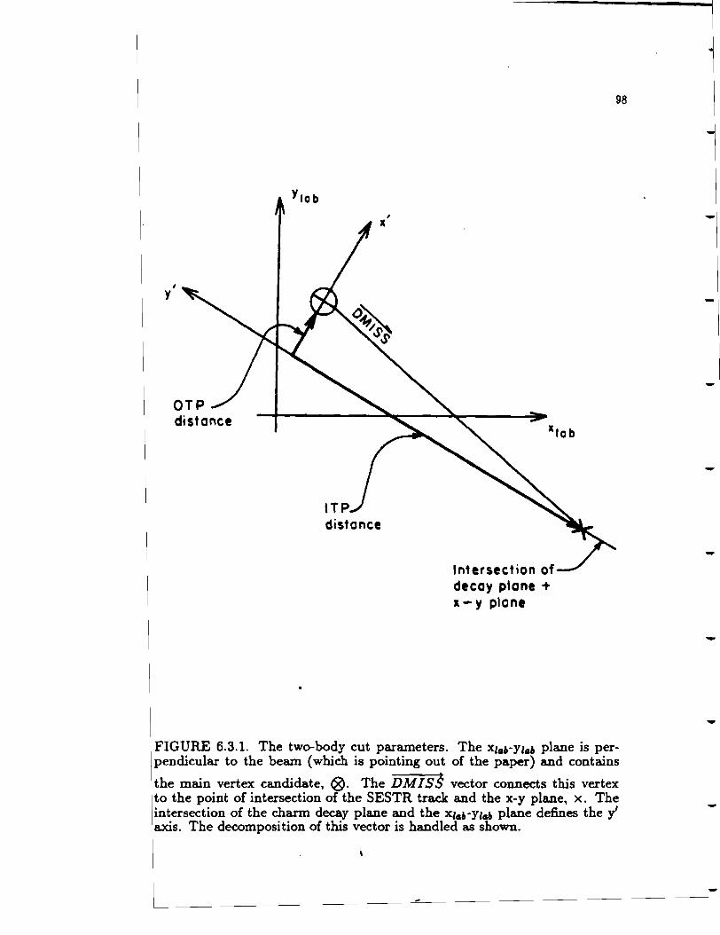
I
y
Yr ob
lTP distance
Intersection of decay plane + x-y plane
98
FIGURE 6.3.1. The two-body cut parameters. The X1a6-Ylo6 plane is perpendicular to the beam (which is pointing out of the paper) and contains
the main vertex candidate, ®· The DMISS vector connects this vertex to the point of intersection of the SESTR track and the x-y plane, x. The intersection of the charm decay plane and the x10 6-Ylo6 plane defines they' axis. The decomposition of this vector is handled as shown.
-
-
-
-
-
-
-
-
-
-
99
approach of the SESTR track and the now well defined charm momentum
direction. As mentioned earlier, this DCA is essentially equivalent to the
OTP distance.* While deriving the DCA with this procedure, we also
obtain the decay distance 6z, which is used in turn to define a two-body
value for the SDZ. The error on the secondary vertex, which is the only
unknown commodity, is given by the ratio of a constant divided by the angle
between the two charm decay products in the laboratory (i.e. the opening
angle). The value of the constant is chosen such that this error effectively
accounts for the measured secondary vertex position error (see figure 6.3.2).
The remaining vertex cut used in the two-body analysis requires the.t the
ITP distance be greater than the OTP distance at all times.
Finally, we can apply a cut on (the cosine of) the angle the SES TR
track makes with the charm particle momentum in the charm particle's cen
ter of mass, defined as coscm( 8). Figure 6.3.3 illustrates the behavior of this
variable for Monte Carlo charm events and data background events. This is
clearly an effective cut variable. The strength of this cut in the /\1r mode
comes from the fact that the charm decay products a.re distributed isotrop
ically in the center of mass of the charm while, in the background events,
hard forward pions ( cos8 = 1) are needed to combine with the A 0 to form
the large A't mass. This cut is important for both two-body modes.
Altogether, then, we have four two-body vertex cuts and the coscm(8)
cut. The most important vertex cut for the A7r analysis was the SDZ cut
while the three other cuts, the RAT (OTP /ITP) cut, the DCA cut, and
* The charm momentum vector is parallel to the charm decay plane and so the minimum distance between this vector and the SESTR track is equivalent to the perpendicular distance from the decay plane to the main vertex. The OTP vector is constrained
to the X-Y plane (since DMISS is) and is in general slightly larger in size than the DCA, but negligibly so.

Cl) 120 &&J -~ 100 t-z &&J 80 ~
0 ~
&&J 40 m ~ 20 z
Cl) 140 .... - 120 ~ t-z 100 .... ~ 80 0 ~ 60 .... m 40 2 ::> 20 z
100
-0.4 -0.2 0 (TRUTH TABLE)-Z
0.2 0.4 (RE CONSTRUCTION)
10 20 30 40 50 I/ (OPENING ANGLE)
FIGURE 6.3.2. These plots were obtained from the two-body analysis of the At - A7r decay mode. The dift'erenc~ between the true secondary vertex position and the decay position obtained from the two-body analysis is plotted in (A), with <r,..,, 700µ. Plot (B) displays the parameter (1/opening angle) which has a mean of,..,, 20. A secondary error of"' .003/(opening angle) ( =.003 x 20. = 600µ on average) is appropriate in this case.
-
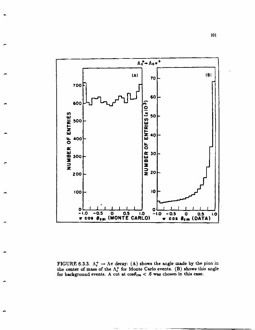
-
-
-
-
-
-
-
101
At•Ao.,,+
(A) 10
(81
700
60 600 -,,,
0 en ~ 50 "' ir 500 en
"' .... ii z .... "' z 40 ~ 400 "' 0 I&. er 0
"' a: 30 m 300 "' 2 m ::> 2 z i 20 200
100 10
o o--...._--....... ___..__--.. ....... _,_--' -1.0 -0.5 0 0.5 1.0 -1.0 -0.5 0 0.5 1.0 ,.. co1 lcin (MONTE CARLO) ,.. co1 '""(DATA)
FIGURE 6.3.3. At - A7r decay: (A) shows the angle made by the pion in the center of mass of the At for Monte Carlo events. (B) shows this angle for background events. A cut at cosScm < ~6 was chosen in this case.
102
the ITP cut were used as background rejection cuts (i.e. they have only a
small impact on charm efficiency, see the efficiency tables in chapter 7). For
the pK0 mode, the proton carried the bulk of the At momentum and thus
degraded the secondary vertex definition. As a result, the ITP cut was the
most important cut for this mode.
The analysis data file for the A 1r mode was created by requiring that
ITP > 0 and jcoscm(8)rl < .7, and by requiring that the SESTR pion have
JCAT ~ 5 (see Table 6.2.1). Again, the cuts had to be applied tightly to
obtain a file of reasonable size ( < 10 K events with an efficiency of 7.53).
The At -+ pKo data file was stripped with similiar cuts as can be seen in
this table, and, in addition, the proton Cerenkov cut was tightened. This
cut was chosen such that only definitely identified protons are accepted (see
figure 6.2.1). The efficiency measured for this strip is "'7.53 and the strip
file contains < 10 K events, the same values obtained for the A1r analysis
strip.
6.4 Monte Carlo Studies
The function of the Monte Carlo is to account for the inability of the
spectrometer to detect all of the signal particles produced in the experiment.
Typically, the spectrometer can fully reconstruct only a few percent of the
charm decays produced in the photon interactions. By accounting for this
inefficiency, we can generate the efficiency corrected charm signal(= N/E
where N =the detected charm signal, and E =efficiency) which is a measure
of the amount of charm produced in this decay mode during the experiment.
In this thesis, we measure t:Pe relative branching fractions of the pKo, A1r,
A1r1r1r, and pKo1r1r decay modes with respect to the more significant pK1r
-
-
-
-
-
-
-
-
-
-
103
decay mode by taking the ratio of efficiency corrected charm signals. This
expression takes the form;
N -RBF = 7(pKo)
/f(pK7r)
for the pKo mode, where RBF = the relative branching fraction. By taking
the ratio of these numbers, we obtain a physically pertinent result which is
independent not only of the sp~ctrometer but of the beam and the charm
production characteristics as well. Systematic problems common to both
modes also tend to cancel. At this juncture, therefore, we need only worry
about how well the Monte Carlo accounts for the differences between the
four modes being studied and the pK7r mode.
The Monte Carlo charm events were generated using the photon
gluon fusion model (section 1.3) and the subsequent gluon and quark frag
ments were hadronized using the Lund fragmentation Monte Carlo. fuJ These
hadrons were propagated through a computer simulation of our spectrometer
where the geometrical acceptance, the resolution, and the intrinsic efficiencies
of the various component detectors were taken into account. In particular,
the Monte Carlo tracking efficiencies were set by measuring the efficiency
of ea.ch individual microstrip and drift chamber plane to fitted tracks from
data charm meson decays with 2, 3, and 4 decay products (D - K7r, K7r7r,
and K7r7r7r). The Monte Carlo tracking efficiencies were set to within 1% of
the values derived from this data (for example, ESMD(planel)= 88 ± 1.5% :
EDc(DlAU)= 93± .6%). The other free parameters in the Monte Carlo, such
88 Cerenkov response, were set in a similiar manner and to similiar accuracy
88 discussed elsewhere. 1211 The Monte Carlo was thus 'tuned' to mimic the
104
data for charm decay modes similiar to those from which these free param
eters were obtained (A°t --+ pK-7r+ for instance). The modes discussed in
this thesis diverge sharply in character from these large statistical samples of
charmed mesons. The presence of a neutral particle in each of these modes
was the most distinct difference, although the behavior of the Monte Carlo
with respect to the Cerenkov cuts and the modified two-body vertex cuts
had to be investigated as well.
The proton Cerenkov cut (nJ was the first cut tested. This was done
by defining clean A 0 data and Monte Carlo samples with cuts similiar to the
A 0 cuts discussed above, excluding the Cerenkov cut. The Cerenkov cuts
were then applied to both samples and, using the pre-Cerenkov A 0 signal to
normalize the results, we obtained well defined efficiencies for these cuts for
both the Monte Carlo and data signals. In this manner, it was determined
that the data was 10% more efficient than the Monte Carlo for the proton
Cerenkov cut used on the pK7r mode. The values for the A7r and A7r7r7r
relative branching fractions derived in this thesis thus had to be increased
by - 10% to account for this difference in efficiencies. The proton Cerenkov
cut applied to the pKO and pK07r7r decays was the same as that applied to
the pK 7r mode a.nd thus no correction was applied to these measurements.
A similiar study of the kaon Cerenkov efficiency using the large charm
meson samples1u
1 showed that a kaon Cerenkov cut that excluded apriori
pions was ,..., 30% less efficient in the Monte Carlo than in the data for
kaons of > 40Ge V / c2 momentum. This problem is closely related to the
problem with the proton Cerenkov cut, as definite Cerenkov identification
of protons begins at 40 GeV /c2 • Less than 10% of the kaons in the pK7r
signal have momentum this high and, therefore, this systematic problem is
-
-
-
-
-

-
-
-
-
-
105
of little concern in the analyses discussed here. These two studies outline the
basic technique used to test the Monte Carlo simulation of data. Clean data
and Monte Carlo samples are first isolated without the use of the cut to be
tested. The efficiency of the cut is then derived separately for the data and
the Monte Carlo and these are compared.
We continue our study of the Monte Carlo with a look at the standard
vertex cuts. Consider figure 6.4.1. The histograms on the left of this figure
show the attenuation of the Monte Carlo signal with respect to the SDZ,
RAT,and DIP cuts for the decay mode D• -+ Do?r -+7rK7r (this was one of
the modes used to develope the Monte Carlo). The plots on the right of
this figure show the efficiency corrected data signal for this decay ( ~ )
with respect to these cuts. This study is possible because we were able to
obtain a data signal in this decay mode without the use of any of the vertex
cuts. We could therefore compare the pre-cut efficiency corrected signal (the
first entry in each plot) to the efficiency corrected signal obtained with the
various vertex cuts. It is clear from this figure that the efficiency corrected
charm signal is stable to within 10% for all cuts. We can assume, then, that
the Monte Carlo is sufficiently stable with respect to these cuts for our study
of the A-tr7r7r and pKo7r7r decay modes since the statistical errors in these
modes are> 25%.
A similiar study of the two-body cuts was then performed using
the same Do -+K7r signal (figures 6.4.2, 6.4.3). First, the kaon (the heavy
particle) was excluded from the vertexing so that this decay would imitate
the A7 -+ ATr decays. The two-body analysis was then performed with the
kaon assuming the role of the A 0 and the pion the role of the pion. The plots
on the right side of figure 6.4.2 show the behavior of the efficiency corrected
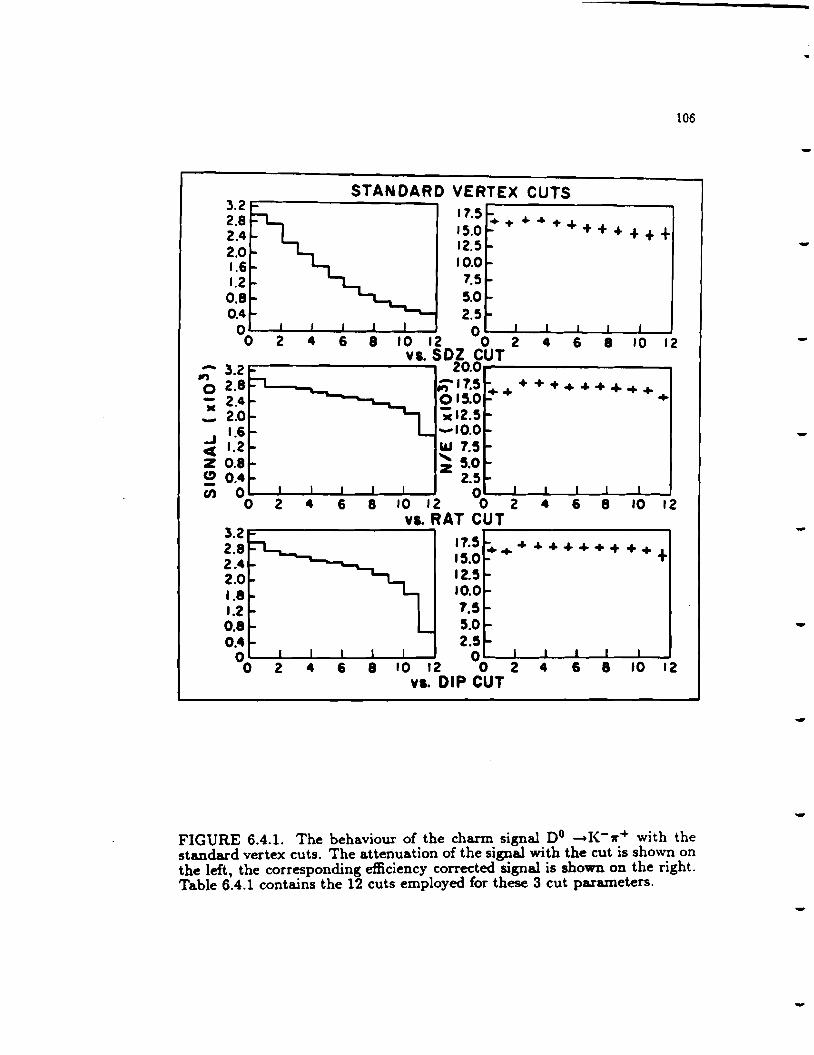
106
STANDARD VERTEX CUTS 3.2 17.5 2.8 ++•~++
2.4 15.0 ++++++ 2.0 12.5
1.6 10.0 1.2 7.5 0.8 5.0 0.4 2.5
0 00 0 2 4 6 8 10 12 2 4 6 8 10 12 VI. SDZ CUT - 3.2 20.0 .,,
0 2.8 ;;11.5 ++••++ ... +•++ JC 2.4 015.0 +
- 2.0 'M 12.5 ..J 1.6 -10.0 c( 1.2 "' 7.5 z 0.8 ' z 5.0 (!) 0.4 2.5 (I) 0 00 0 2 4 6 8 10 12 2 4 6 8 10 12
v1. RAT CUT 3.2
17.5 2.8 ........... +++++++ 2.4 15.0
2.0 12.5 1.8 10.0 1.2 7.5 0.8 5.0 0.4 2.5
00 2 4 6 8 10 12 00 2 4 6 8 10 12 va. DIP CUT
FIGURE 6.4.1. The behaviour of the charm signal o0 -K-1r+ with the standard vertex cuts. The attenuation of the signal with the cut is shown on the left, the corresponding efficiency corrected signal is shown on the right. Table 6.4.1 contains the 12 cuts employed for these 3 cut parameters.
-
-
-
-
-
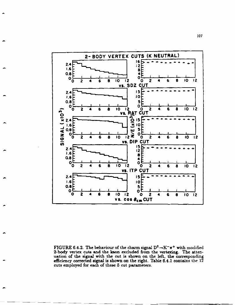
-
-
-
-
107
2- BODY VERTEX CUTS (K NEUTRAL) r::rs;;: J :!f -,-·.-·,-·.· ·.··1 0 o 2 4 6 8 10 12 0 2 4 6 8 10 12
VI. soz C.,.;;;U...;.T _______ _,
r::r=:------, --, ---~--. :~r -,- ·,· ·.- -,- -.- ·1 -
0o 2 4 6 8 10 12 °o 2 4 6 8 10 12
0 vs. RAT c_u_T _______ ....,
~lit. I I ::g~:ff·,·•lhl++!++l++I = 0 2 4 6 8 10 12Z 0 2 4 6 8 10 12
<n 2.4~vs. o•:t~:-. -. --. •. • 1.6 8 ~ 0.8 4 ~
0 O"" I I I I I
0 2 4 6 8 10 12 0 2 4 6 8 10 12 VI. ITP CUT
!:i[r----::--~--:J---- :if~-.-.-----1---.. -.. -.-,.-.-,.-...... 1
0o ~ 4 6 8 10 12 0 2 4 6 8 10 12 v I. COi 'Cl" CUT
FIGURE 6.4.2. The behaviour of the charm signal o0-K-w+ with modified 2-body vertex cuts and the kaon excluded from the vertexing. The attenuation of the signal with the cut is shown on the left, the corresponding efficiency corrected signal is shown on the right. Table 6.4.1 contains the 12 cuts employed for each of these 5 cut parameters.

2-BODY VERTEX CUTS (Pl NEUTRAL)
2.4t:;;:J 16 ~ - •• - - •• + 16
12~ ••• . e:
1.8 4 = 0 "" I I t t I
0 2 4 6 8 10 12 °o 2 4 6 8 10 12 ............ --~-~~~v~s.SDZCUT t::C ~ :~~i:::--.-.-.. -.. -.--.-•• -.I
;; 0~ ~ ~2 °t 2 4 ~ ~ .~ 12
o vs. RAT CUT
• 2 ·4rr------~---.... ;:;--~ :; -=:::r---.-.-.---.-.-.---.-.1 ~~:: " z 0- I I I ~ 0 I I I I I C!> 0 2 4 • 8 10 12 z 0 2 4 6 8 10 12 en VI. DIP CUT 2.•c-:------~------ :~ ... = ... -.---.. -.-.. -.---.-... -.-.-1.6 8: 0.8 4::
0 o"" I I I I 1
0 2 4 6 8 10 12 0 2 4 6 8 10 12 vs. ITP CUT
!:o:~----.-.--.---~-~------- :~[---.. -.. --.-.. ---.. --.-.--.-.--.!
0- 2 4 6----al0!2 °o 2 4 ~ ~ 10 12 VI. cos le"' CUT
108
FIGURE 6.4.3. The behaviour of the charm signal o0-K-w+ with modified 2-body vertex cuts and the pion excluded from the vertexing. The attenuation of the signal with the cut is shown on the left, the corresponding efficiency corrected signal is shown on the right. Table 6.4.1 contains the 12 cuts employed for each of these 5 cut parameters.
-
-
-
-
-

-
-
-
-
109
charm signal with respect to vertex cuts on the pion. This signal is stable
for all cuts to within 10%. The pion was then excluded from the vertexing so
that the behavior of the charm signal would more effectively mimic the A"t -+
pK0 mode. The plots on the right side of figure 6.4.3 shows the efficiency
corrected signal with respect to the vertexing cuts on the kaon. Again, the
signal is stable with respect to these cuts to within 10%.
The values of the cuts used in the plots contained in figures 6.4.1-3
are listed in table 6.4.1. There are twelve cuts listed for each cut parameter
as there are twelve entries in each of the plots in these figures. The cuts that
are listed in this table naturally correspond one to one to the plot entries.
As can be seen in the plots, the cuts are tightened with each succeeding cut
value except in the coslJ plots where there are two sets of cuts investigated.
In this case, the first set of cuts is applied to the cut variable coslJ (No
Vtx(~No vertex cuts), NVV> 0 (~Main vertex exists), .9, .8, .7, .6, .5) and
the second set (.9, .8, .7, .6, .5) is applied to the parameter lcos8 I. The final Monte Carlo tests were on the stability of the cuts used to
define the neutrals (see section 6.1.1 and figure 6.1.1) and on the tracking
efficiency of the neutral particle decay products. Figure 6.4.4 shows the K,
and A 0 efficiency corrected signals as a function of the neutral particle vertex
cuts. As before, the efficiency corrected signal for both neutrals is stable with
respect to these cuts to < 10%.
The tracking efficiency of the neutral particle decay products is tested
using large statistic charmed meson decay modes and, independently, using
K•0 and K•+ signals. The study is discussed in Appendix A. In the study,
efficiency correction factors were generated as a function of the beam energy
------ --------------- ---------------

110
0 4.5 'iC - + _, 4.0 er 3.5 z (!) 3.0 -
+ -+ (A)
--+-(/)
0 2.5 < 2.0 a: 1.5 ~
0 1.0 u u 0.5 u 0 <
-2 3
vs. Ao NEUTRAL CUTS ,,, E 20.0 CB l • - 17.5 _, < 15.0 z (!) '2.5 -(/)
en 10.0
2 3 4
vs. KsHORT NEUTRAL CUTS
FIGURE 6.4.4. These plots show the stability of the Monte Carlo with respect to the neutral particle cuts; plot (A), the As and plot (B), the K,,s. The cuts are outlined in figure 6.1.1 which also shows the data signals used to generate these plots.
-
-
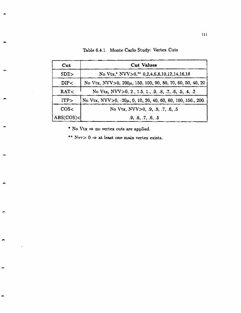
111
-Table 6.4.l. Monte Carlo Study: Vertex Cuts
Cut Cut Values
SDZ> No Vtx: NVV>o:• 0,2,4,6,8,10,12,14,16,18
DIP< No Vtx, NVV>O, 200µ, 150, 100, 90, 80, 70, 60, 50, 40, 20
RAT< No Vtx, NVV>O, 2., 1.5, 1., .9, .8, .7, .6, .5, .4, .2
ITP> No Vtx, NVV>O, -20µ, 0, 10, 20, 40, 60, 80, 100, 150., 200.
COS< No Vtx, NVV>O, .9, .8, .7, .6, .5
ABS( COS)< .9, .8, .7, .6, .5
* No Vtx => no vertex cuts are applied.
** Nvv> 0 =>at least one main vertex exists.
-
-
-
112
and the slope of the K, momentum vector, *(K,). The K• generated cor
rections presented in table 6.4.2 were used to correct the four charm modes
and are applied in the final analysis (chapter 7). It should be noted that the
reliability of the K• corrections depends crucially on the relative production
of the K•+ and the K•0 •
-
-
-

113
-Table 6.4.2. Neutral Particle Efficiency Corrections
Decay Mode Correction
ATr7r7r /pK7r 1.4 ± .4
A7r/pK7r 1.3 ± .3
pKo/pKTr 1.2 ± .3
At ~ pKo7r7r 1.3 ± .3
CHAPTER 7
RESULTS
In this chapter, the final set of cuts for each of the charm decay
modes, Arrrrrr, Arr, pKo, and pKorrrr, is outlined and the relative branching
fractions for each of these modes relative to the pKrr mode is derived. These
results are then compared to the theory where such predictions exist. A
discussion of the possible decay mechanisms of the At follows.
7 .1 The Normalizing Mode: At--+ pK 7r
The At--+ pKrr decay mode has been discussed elsewhere. 1441 We use
this mode as the denominator in the calculation of the relative branching
ratios reported in this thesis as it is the most significant At signal seen in
our experiment. The full complement of cuts were used to extract this signal.
We apply a DIP cut of 80µ, an SDZ cut of 6., a RAT cut of 1.5, as well as
Cerenkov cuts of 70% on the pion probability, 80% on the proton probability,
and 50% on the kaon probability. The pion momentum must be greater than
3 GeV /c2 as well. The signal is shown in figure 7.1.1. The Cerenkov cuts
were chosen not simply to enhance the significance of the signal but to match
the Cerenkov cut applied to the pKO mode. The systematic error introduced
by the proton efficiency correction will therefore not be included in this (or
the pKOrrrr) decay mode.
The raw signal obtained in the pKrr decay mode is 134 ± 17 which
implies an efficiency corrected signal of 6674 ± 885, given the 2.0 ± .13
efficiency of these cuts. The width of this fit is constrained to be 9 MeV /c2 ,

-
-
-
-
-
115
which is the width of the Monte Carlo signal, and the mass is measured to
be 2.286± .002 GeV /c2 • ·Applying the Cerenkov corrections discussed in the
last chapter (Kaon Correction= 1.02± .02: Proton Correction= 1.11 ± .11)
to this mode we get the 'corrected' efficiency corrected signal,
A( K ) = 667 4
± 885
= 5900 ± 780 ± 800 p 71' 1.13 ± .13
where the systematic error introduced by the fit ( 4 % ) is included in the
calculation.
It is important to note here that the Cerenkov cuts applied to the
pK11' mode constrain the charm momentum to be > 40GeV /c2 • In like
manner, the charm signal in decay modes containing neutrals is negligible . above 120 GeV /c2 because of the difficulties involved in reconstructing high
momentum neutrals. All the At signals reported in this thesis therefore
have their momenta constrained between [40-120GeV /c2 ] so that the charm
signals are compared in similiar charm momentum regions.
7.2 The At -+ A11'+71'-71'+ Signal
The analysis on the A11'71'71' mode was performed as follows. The
vertex cuts used to extract the signal were the DIP cut, the RAT cut, the
SDZ cut, and the x;ec/DoF cut. These were applied to the charm vertex, as
formed by the three pions, at the values shown in table 7.2.1. The momenta
of the three pions was also constrained to be greater than 2 Ge V / c2 . The
values of these cuts were chosen by maximizing the quantity SIG= Ji"'c DATA
which measures the significance of the A11'11'7r Monte Carlo signal, SMc, with
respect to the background, BDATA, found in the data with the same cuts.
Figure 7.2.1 illustrates how the value of the SDZ cut for the A7r11'7r mode was
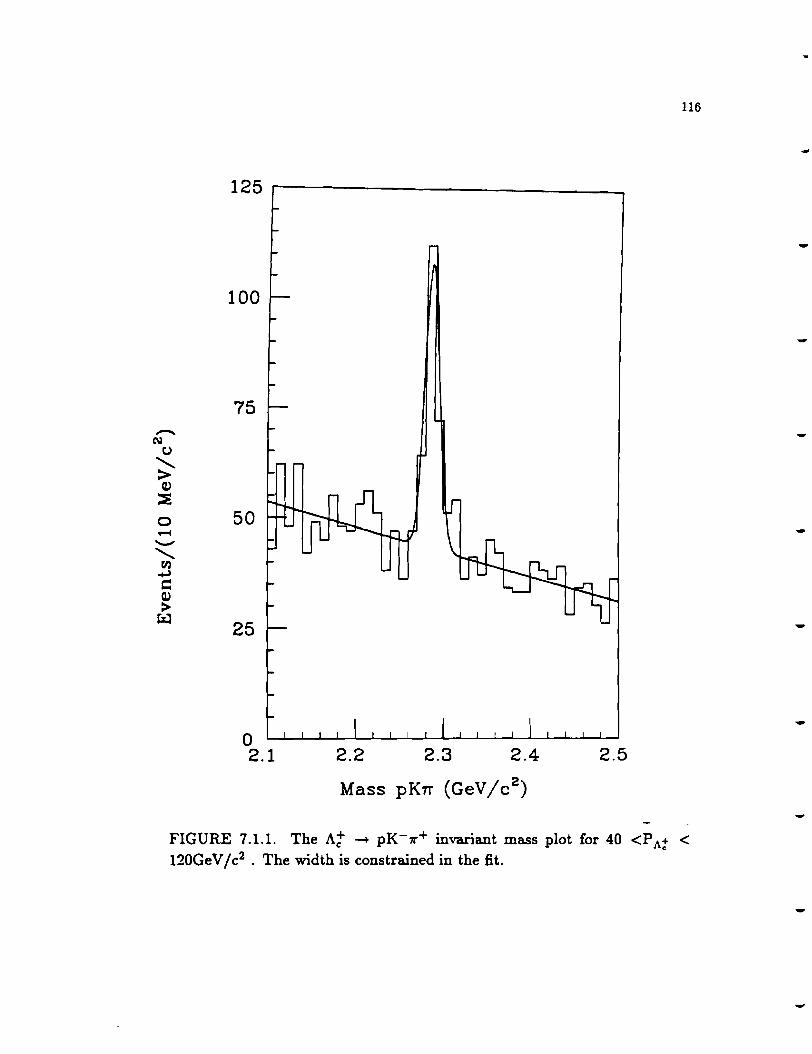
-N t.>
.......... > Q)
:e 0 ..-4 ....._
.......... rn ...., r:: Q)
> ril
100
75
50
25
0 2.1
116
2.2 2.3 2.4 2.5
Mass pKrr (GeV / c 2)
FIGURE 7.1.1. The At - pK-1r+ invariant mass plot for 40 <P At < 120GeV /c2 • The width is constrained in the fit.
-
-
-
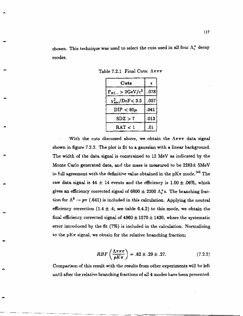
-
-
-
-
117
chosen. This technique was used to select the cuts used in all four At decay
modes.
Table 7.2.1 Final Cuts: A7r7r7r
Cuts E
Pr1... > 2GeV /c2 .078
x;ec/DoF < 3.5 .057
DIP< 80µ .041
SDZ > 7 .013
RAT< 1 .01
With the cuts discussed above, we obtain the A7r71"7r data signal
shown in figure 7.2.2. The plot is fit to a gaussian with a linear background.
The width of the data signal is constrained to 12 MeV as indicated by the
Monte Carlo generated data, and the mass is measured to be 2283± 5MeV
in full agreement with the definitive value obtained in the pK7r mode.101 The
raw data signal is 44 ± 14 events and the efficiency is 1.00 ± .06%, which
gives an efficiency corrected signal of 6800 ± 2200 A"t s. The branching frac
tion for A 0 -+ p7r ( .641) is included in this calculation. Applying the neutral
efficiency correction (1.4 ± .4; see table 6.4.2) to this mode, we obtain the
final efficiency corrected signal of 4860 ± 1570 ± 1430, where the systematic
error introduced by the fit (7%) is included in the calculation. Normalizing
to the pK7r signal, we obtain for the relative branching fraction;
RBF ( ~;;;) = .82 ± .29 ± .27. (7.2.2)
Comparison of this result with the results from other experiments will be left
until after the relative branching fractions of all 4 modes have been presented.
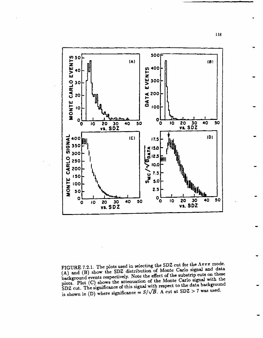
118
en so 500 ~ t- (A) z CB l
LIJ 40 en 400 .... > t-LIJ z 0 30 la.I 300 ... ..J > a: LIJ
~ 20 <200 ... t-
LIJ < t- 10
Q
z 100-
0 I
2 0 " I I I 0 0 10 20 30 40 50 0 10 20 30 40 50
vs. SDZ VI. SOZ
..J • 4(400 1,
(C) 17.5 (0)
~ 350 ~~ - ~·s~ en 300 I g 250 I ~ 12.5
II \ ~ 200 1, 10.0
(.) ........
LI.I 150 '\, u 7.S ~ 2 t- 100 en 5.0
~-d z ., 0 50 ' .... 2.5 2
0 00 0 10 20 30 40 50 10 20 30 40 50
vs. S DZ vs. SDZ
FIGURE 7.2.1. The plots used in selecting the SDZ cut for the A-rrtrtr mode. (A) and (B) show the SDZ distribution of Monte Carlo signal and data background events respectively. Note the effect of the substrip cuts on these plots. Plot (C) shows the attenuation of the Monte Carlo signal with the SDZ cut. The significance of this signal with respect to the data background is shown in (D) where significance= S/../B. A cut at SDZ > 7 was used.
-
-
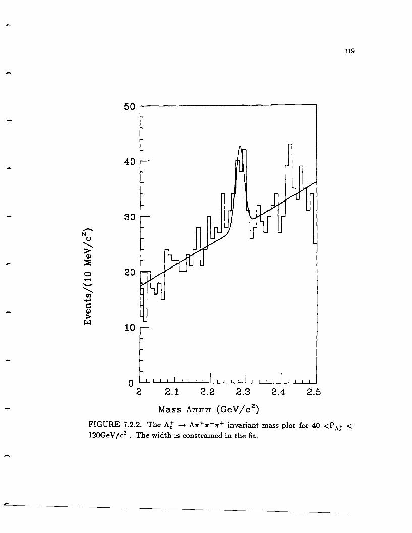
-
-
-
119
40
30 -N C.>
.......... > Q)
~
0 20 --.......... I'll
.,J
c:: Q)
> t;:J
10
0 2 2.1 2.2 2.3 2.4 2.5
Mass Arrrrrr (GeV /c 2)
FIGURE 7.2.2. The At -+ A1r+1r-1r+ invariant mass plot for 40 <P At < 120GeV /c2 . The width is constrained in the fit.

120
7.3 The At - A11'+ Signal
The analysis of the A 11' mode differs greatly from the analysis of the
A11'11'11' mode, as was discussed earlier. The vertex cuts used for this mode
are the modified SDZ and RAT cuts, the DCA cut, and the coscm( 8) cut
discussed in section 6.3; their values are given in table 7.3.1. These cuts
were chosen by maximizing the significance of the A11' Monte Carlo charm
signal with respect to a background derived from the data, as for the A11'11'71'
mode. The plots used to select the SDZ cut value for this mode are shown
in figure 7.3.1. Comparing this plot qualitatively to figure 7.2.1 illustrates
the improvement one could expect if a standard secondary vertex could be
defined for the A 11' mode.
Table 7.3.1 Final Cuts: A11'
Cuts E
lcoscm( B)r I < .6 .095
ITP > 30µ .048
DCA < 80µ .043
SDZ >2 .037
RAT< .75 .034
The A 11' data signal obtained by applying the cuts outlined in table
7.3.1 is shown in figure 7.3.2. The plot is fit to a gaussian plus a linear
background function. The width and mass are both constrained; the width
to 13 Me V, the value indicated by the Monte Carlo, and the mass to 2.286
GeV /c2 as indicated by the strong pK11' signal. The raw data signal obtained
is 28 ± 13 events and the efficiency is 3.4 ± .2%, implying an efficiency
corrected At signal of 1280 ± 600. The branching fraction for A 0 - p11' is
included in this calculation. Applying the neutral efficiency correction {1.3 ±
-
-
-
-

-
-
-
-
-
-
121
120 Cl) I- 100 (A) I B) z 100
"" Cl)
> 80 I-
"" z 80 0 "" ..J 60 > a: "" 60 c c (,) 40 I- 40
"" c
I-20
0 z 20 0 ~
0 0 -20 -10 0 10 20 -20 -10 0 10 20
vs. soz vs. soz Cl) 35 + I- 500 HllHllHIHtHtH
1 (Cl (0) z
~ "" > ~ 25
""400 0 t t
. ~ 300 20 c
~ 15
'1 (,)
""200 2 I- Cl) 10 z t\ 0 100 I
~ • 5
0 ••• \ttt.
0 -20 -10 0 10 20 -20 -10 0 10 20
VI. SOZ vs. soz
FIGURE 7.3.1. The plots used in selecting the SDZ cut for the A7r mode. (A) and (B) show the SDZ distribution of Monte Carlo signal and data background events respectively. Plot ( C) shows the attenuation of the Monte Carlo signal with the SDZ cut. The significance of this signal with respect to the data background is shown in (D) where significance = S /VB. A cut at SDZ > 2 is indicated here.

122
50
40
-N CJ
30 .......... >
Q,)
::s 0 ..-4 -.......... 20 en ....., r= Q,)
> r.;;;i
10
0 2 2.1 2.2 2.3 2.4
Mass Arr (GeV /c 2)
FIGURE 7.3.2. The At -+ A7f'+ invariant mass plot for 40 <P At < 120GeV /c2 • The width and mass are constrained in the fit.
-
-
-
-
-
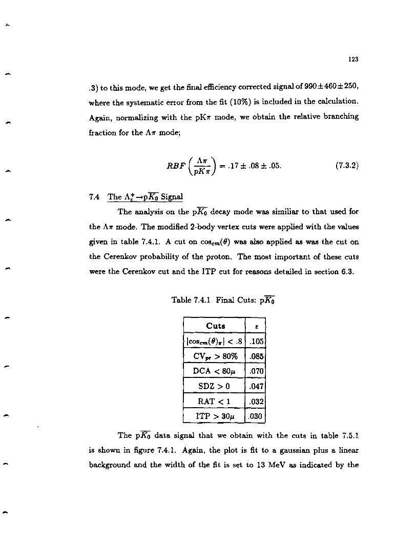
-
-
-
-
-
-
-
-
-
123
.3) to this mode, we get the final efficiency corrected signal of 990±460±250,
where the systematic error from the fit (10%) is included in the calculation.
Again, normalizing with the pK7r mode, we obtain the relative branching
fraction for the A7r mode;
RBF (~7r7r) = .17 ± .08 ± .05. {7.3.2)
7.4 The At-+pKQ Signal
The analysis on the pKo decay mode was similiar to that used for
the A7r mode. The modified 2-body vertex cuts were applied with the values
given in table 7.4.1. A cut on coscm(8) was also applied as was the cut on
the Cerenkov probability of the proton. The most important of these cuts
were the Cerenkov cut and the ITP cut for reasons detailed in section 6.3.
Table 7.4.1 Final Cuts: pK o
Cuts f
jcoscm{8) ... I < .8 .105
CVJW" > 80% .085
DCA < 80µ .070
SDZ > 0 .047
RAT< 1 .032
ITP > 30µ .030
The pKo data signal that we obtain with the cuts in table 7.5.1
is shown in figure 7.4.1. Again, the plot is fit to a gaussian plus a linear
background and the width of the fit is set to 13 MeV as indicated by the
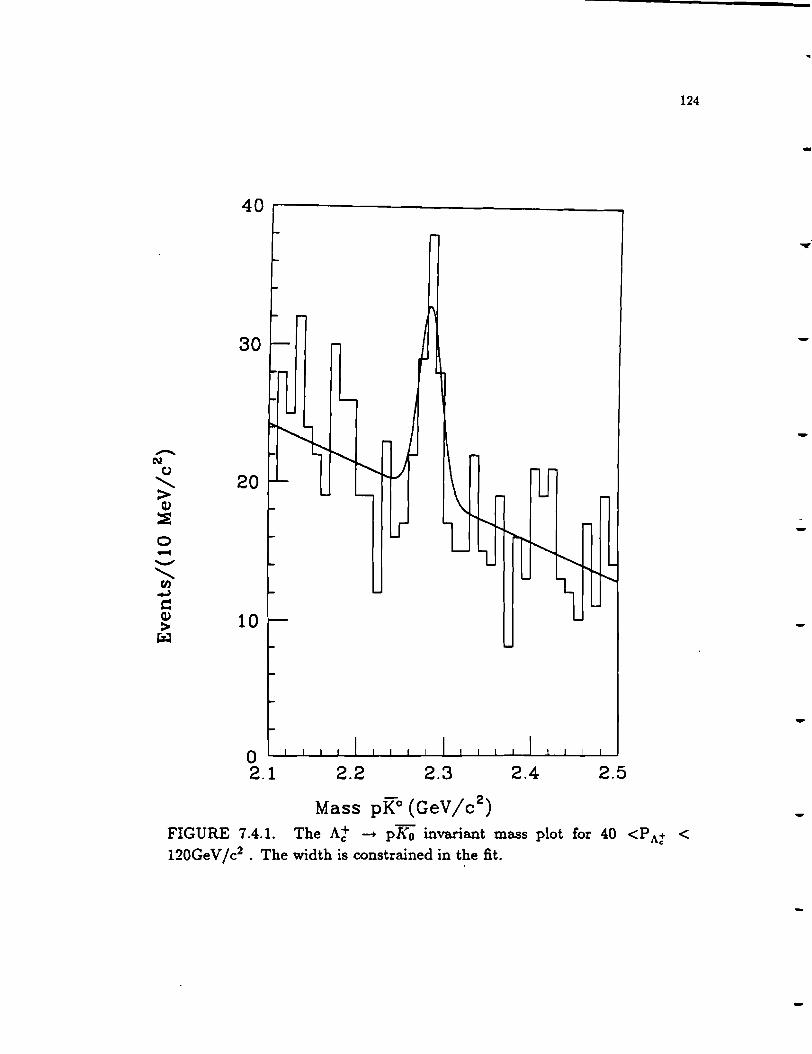
-N tJ
........... > Q)
:::s 0 --........... rlJ ~
c:: Q)
> ~
30
20
10
0 2.1
124
2.2 2.3 2.4 2.5 - 2 Mass pK0 (GeV /c )
FIGURE 7.4.1. The At -+ pKo invariant mass plot for 40 <P At < 120GeV /c2 • The width is constrained in the fit.
-
...

-
-
-
-
-
-
125
Monte Carlo. The mass is measured to be 2283 ± 3 Me V, which is consistent
with the pK7r mode. The raw data. signal we obtain is 45 ± 12 events and
the efficiency for this decay mode is 3.0 ± .2%, giving an efficiency corrected
A"d signal of 4350 ± 1190. The branching fractions of K 0 -+ K6 (.5) and
K 6 -+ 11"+11"- (.686) are included in this calculation. Applying the neutral
efficiency (1.2 ± .3) and the proton Cerenkov (1.11 ± .11) corrections, we get
the final efficiency corrected signal of 3270 ± 890 ± 900, where the systematic
error for the fit ( 5%) is included in the calculation. Note that the contribution
to the systematic error from the proton Cerenkov correction is cancelled when
this mode is normalized to the pK11" mode. The relative branching fraction
obtained is then;
(pKo) RBF pK1r = .55 ± .17 ± .14. (7.4.2)
7.5 The At-+pKcl1r+1r- Signal
The analysis of the pKo7r7r mode proceeded in the same way as the
analysis of the /\7r7r7r mode since we were able to define a standard secondary
vertex with the p7r7r SESTR tracks. The cuts and their values are given in
table 7.5.1. Comparing these cuts with the cuts used in the /\7r11"11" analysis
(see table 7 .2.1 ), we can see the similiarity between the behavior of signal and
background in these two modes. The ma.in difference in their analyses is the
Cerenkov cut on the proton probability, CV prr > .25 which, as noted earlier
(see section 6.3), excludes all but definitely identified proton candidates.

126
Table 7.5.1 Final Cuts: pKo7r7r
Cuts f
CVprxCVr1 xCVr2 > 25~ .050
Pr1 ... > 2GeV /c2 .043
X~ee/ dof < 3.5 .028
DIP< 80µ .020
SDZ > 7 .006
RAT< 1 .004
The pKo7r7r data signal is shown in figure 7.5.1. The width of the
fit is set to 10 Me V as indicated by the Monte Carlo and the mass is set
to the pK7r value of 2.286 GeV /c2 . The plot is fit to a gaussian plus a
linear background. The raw data signal is 9 ± 6 events and the efficiency
for this mode is .4 ± .043, implying an efficiency corrected At signal of
6700 ± 4500. The branching fractions of K 0 -+ K. and K. -+ 7r+7r- are
included in this calculation. Applying the neutral efficiency {1.3 ± .3) and
proton Cerenkov {1.11 ± .11) corrections, we get the final efficiency corrected
signal of 4600 ± 3300, where the systematic and statistical errors have been
combined. Normalizing this result to the pK7r mode, we obtain the limiti
(7.5.2)
As with the pKO mode, the proton Cerenkov correction does not contribute
to the systematic error used in this measurement.
-
-
-
-
-

-
-
-
-
-
127
12 I-
....
.... t-
10 - .. --I-
I-
B - .... I-
... .. ...v I-........... ,. ~
N I- v C) ... ~ .......... 6 - ..
i..-" =-> J \.i-'
Q) -::; t- ,,./ -0 I- ~i..-"
I-'~ ....... t-
... ~v ... -.......... 4 ... ... ......i..-"
rn ... vi..--...,i
c:: ... ~ Q)
... --> ~
2 ... .
.. .. ...
I I I I I I I I I I I I I I I I I I I I I I
... 0
2 2.1 2.2 2.3 2.4 2.5
Mass pKcn-11' (GeV / c 2)
FIGURE 7.5.1. The At -+ pKo?r+?r- invariant mass plot for 40 <P At < 120GeV /c2 • The width and mass are constrained in the fit.

CHAPTERS
RESULT COMPARISONS AND CONCLUSIONS
The relative branching fractions derived in the previous chapter are
insensitive to the details of our experiment. We can therefore compare these
values to similiar measurements ma.de by other experiments. I will restrict
my comparison with experiment to the results from CLEO and ARGUS, with
some results from MARKII where applicable. A discussion of the theoretical
results follows this.
Table 8.1.1 contains the results reported in this thesis a.long with
previously existing results from the e+e- experiments, CLEO, 101 ARGUS, !tel
and MARKII. !•Tl It is clear that our results agree with ea.ch of the oth~r
results, providing corroboration for these earlier measurements. It should
be noted that these are the first significant measurements of At relative
branching fractions from a. fixed target experiment.
The discussion of theoretical predictions for these rates will be re
stricted to the two body modes because these are the only decays that have
been calculated. These predictions have been presented most conveniently
in the form ( r(Ar) =) RBF(Air /pK0 ) by Ebert and Kallies.c131 The experi-r(pK0)
mental value we obtain for this parameter is .3 ± .2, which naturally agrees
with the values obtained by CLE0(.33) and ARGUS(< .27). Table 8.1.2
contains a. comparison of our experimental result with available theoretical
predictions. It is apparent that the SU(4), current algebra., and quark model
..
-
-
-
-
-
-
-
-
-
-
-
129
calculations agree with our result while the MIT Heavy Bag Model calcula
tion disagrees.
The symmetry and quark model calculations were done by Korner,
Kramer, and Willrodt. 1111 In the SU(4) calculation, we consider the SU(2)
I( =lsospin), U, and V spin subgroups, where;
I+d = u; U+s = d; V+s = u
I+ti= -d;U+d= -s;V+ti= -s.
It is apparent that the effective hamiltonian (given in equation 1.2.1 and
1.2.2) transforms as an I or U spin vector, implying that the baryon decays
obey the selection rules, A/ = AU = 1. The two separate parts of this
hamiltonian transform differently under V spin; the o- part in equation
1.2.2 transforms as a V spin scalar (AV= 0) while the o+ part transforms
as a V spin vector (AV= 1). Korner et. al. applied the A/= AU= 1 and
AV = 0 properties of the hamiltonian to I, U, and V spin meson a.nd baryon
multiplets to obtain sum rules relating different AC= 1 decays to each other.
The AC = .1 decays were then related in the same manner to known AC = 0
( J""'~-1
(411) decays and scaled by the ratio of enhancement factors /
= 0.54 ) to
obtain the estimate for the decay rate entered in column 2, table 8.1.2.
The decay amplitude used in the quark model calculation was derived
from the effective hamiltonian (again, see equation 1.2.1) and is essentially
the same as that obtained using current algebra. tii1J In this calculation, the
contribution to the rate from the W-exchange and W-emission diagrams is
generated by inserting quark model wavefunctionsruJ explicitly into this am
plitude, where the wavefunction overlap, the ratio of enhancement factors,
etc. are estimated from the known behavior of AC = 0 decays. The contri
bution to the rate from the spectator diagrams is then derived in terms

130
of the measured current transition form factors of established baryons. These
two amplitudes are added to get the relative branching fraction estimate
entered in column 3, table 8.1.2.
Only the first term in the effective hamiltonian (equation 1.2.1) is
used in the current algebra calculation. 11 ~1 Soft meson technique plus current
algebra are used to reduce the three hadron matrix element to calculable
baryon to baryon transition elements. The tlC = 1 baryon transitions ele
ments in these expressions are then related to tlC = 0 transition elements
using symmetry considerations. Adding in the spectator contribution as be
fore, we obtain the value for the relative branching fraction entered in column
4, table 8.1.2.
The same soft meson plus current algebra method is used in the MIT
Heavy Bag Model calculation to derive the baryon decay amplitude. The
charm quark wavefunction is taken to be gaussian with u 2 ,..,, 1/M~ and the
recoil of the charm quark with respect to the light quarks is neglected. The
charm quark is thus centered in the bag. The masses and frequencies assigned
to the light quarks in this calculation are the standard values1"
1 and, adding
in the spectator contribution, we obtain the value for the relative branching
fraction entered in column 5, table 8.1.2. This method is inconsistent with
our experimental result because it underestimates the At -+ pK0 decay rate.
The future prospects for experimental measurements of these, and
other, At relative branching fractions are bright. CLEO and ARGUS have
both taken more data since they submitted the results presented in this
thesis, so significant improvement in their measurements of these ratios can
be expected soon. Photon experiments (with hopes of taking 109 events)
-
-
-
-
-
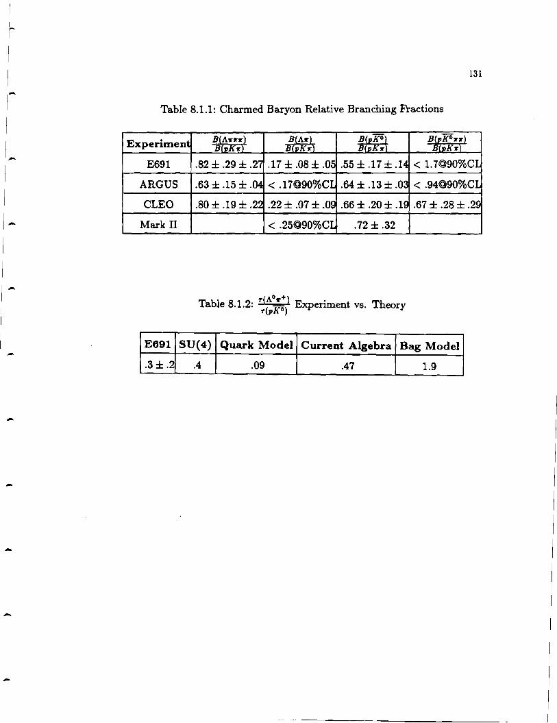
131
Table 8.1.1: Charmed Baryon Relative Branching Fractions
Experimen
E691 < 1.7@90%C
ARGUS < .94@90%C
CLEO
Mark II < .25@90%C .72 ± .32
r(A0 r+) . Table 8.1.2: r(pKo) Experiment vs. Theory
E691 SU(4) Quark Model Current Algebra Bag Model
.3±.2 .4 .09 .47 1.9
-
-

132
and very high statistic fixed target hadron experiments also figure in the
future of baryon physics~ The most promising experiments of all, however,
will most probably be the Z0 factories gearing up at CERN and SLAC. The
determination of all pertinent measurements involving the charmed baryons
may well be at hand. The theoretical prospects are not this bright but, as
the experimental results increase, so will the theorist's interest.
-
-
-
-
-
-
-

-
-
-
-
-
-
REFERENCES
1. Gell-Mann, M., Phys. Rev. Lett. 8, 214 (1964).
2. Particle Data Group; Phys. Lett., 1 TOB 1 1986.
3. Greenberg, O.W., Phys. Rev. Lett. 13, 598 (1964).
4. Gross, D.J., Wilczek, F., Phys.Rev.Lett. 30, 1343 (1973); Politzer, H.; Phys. Rev. Lett. 30, 1346 (1973).
5. Trilling, G; The Properties of Charmed Particles; Physics Reports 15 no.2 (1981).
6. Glashow, S.L., Ilioupoulos, J ., Maiani, L; Phys Rev D 2 1285 (1970).
7. Halsen and Martin; Quarks and Leptons, (John Wiley and Sons) 1984.
8. Gross, D.J., Wilczek, F., Phys. Rev. D8, 3633 (1973); Phys. Rev D9, 980 (1974), Politzer, H.D. Phys. Rep. 14C, 129 (1974).
9. Quigg, C., Kwong, W., Rosner, J.; Heavy Quark Systems, FermilabPub-87 /15-T.
10. Santoro, A., Souza, M., Escobar, C.; Notes about Lambda/c, E691 Internal Memo.
11. Komer, J.G., Kramer, G., Willrodt, J.; Zeit. fur Phys. C Particles and Fields 2, 117 (1979).
12. Ellis, J., Gaillard, M.K., Na.nopoulos, D.V.; Nucl. Phys.; BlOO 313, (1975).
13. Ebert, D., Kallies, W.; Zeit. fur Phys. C, Particles and Fields 29, 643 (1985).
14. Delbargo, R., Salam, A., Strathdee, J .; Proc. Roy. Soc. A278, 146 (1965).
15. Hussain, F.,Scadron, M.D.; II Nuovo Cimento 79A, 248 (1984)
16. Jones, L., Wyld, H.; Phys Rev Dl 7 759 (1978).
17. Holmes, S., Lee, W., Wiss, J .; Ann. Rev. Nucl. Part. Sci. 35, 397 (1985).
18. Seyward, H; PhD Thesis; University of Toronto (1987).
134
19. Gaillard, M.D., Lee, B.W., Rosner, J.; Rev. of Mod. Phys., Vol 47, No. 2, (1975).
20. Bhadra, S; PhD Thesis; University of Colorado, Boulder (1984).
21. Tsai, Y; Rev. Mod. Phys.; 46, 815 (1974).
22. Raab, J; PhD Thesis; University of California, Santa Barbara (1987).
1t1./2 z2dz 23. The intrinsic resolution of this detector is <rlnt = t1.IJ,2 = <fl /12.
Jtl.12 dz
24. Browder, T; PhD Thesis; University of California, Santa Barbara (1988).
25. Damerell, C; Vertex Detectors In Ferbel, T (editor); Techniques and Concepts of High Energy Physics IV, Chapter 8; Plenum Press (1987).
26. Mena.ry, S; Ms Thesis; University of Toronto (1986).
27. Jackson, J; Classical Electromagnetism, (John Wiley and Sons) 1975.
28. RCA Corporation, Lancaster, Penn., USA.
29. Bartlett, D.F. et al; Nucl. Ins. and Meth. A260 55 (1987).
30. Eagle Convex Glass Co., 419 Tuna St., P.O. Box 1340, Clarksburg, West Virginia, 26301, USA.
31. Acton Research Corp, 525 Main St., Acton, Mass., 01720, USA.
32. Carlson, P.J.; Nucl. Instr. and Meth., 158 403 (1979).
33. LeCroy Corp., 700 S. Main St., Spring Valley, N.Y., 10977, USA.
34. Bartlett, D.F.; Duncan, A.L.; Elliot, J.R.; Rev. Sc. Inst. 52 265 (1981).
35. Amersil Inc.; 650 Jones Road, Sayreville N.J., 08872, USA.
36. Summers, D; PhD Thesis; University of California, Santa Barbara (1984).
37. Mathews, J., Walker,R.L.; Mathematical Methods of Physics, (Benjamin, Menlo Park, California) 1970.
-
-
-
-
-
-
-
-
-
-
-
-
135
38. The apriori likelihoods for electrons, muons, pions, kaons, and protons used are .02, .01, .81, .12, .04 respectively.
39. The A and Ka strips differed because they were done by two different people. The slight differences in the cuts did not affect the charm signals.
40. Goldstein, H.; Classical Mechanics; (Addison-Wesley) 1950.
41. Sjostrand, T.; LU TP 85-10.
42. Cremaldi, L.M.; E691 Internal Group Memo, May 1988.
43. Sokoloff, M.D.; E691 Internal Group Memo, Jan 1988.
44. Anjos, J.C., et al; Phys. Rev. Lett.; 60 1379 (1988)
45. Alam, M. et al.,, 1987 International Symposium on Lepton and Photon Interactions at High Energies, Hamburg.
46. Albrecht, H. et al., 1987 International Symposium on Lepton and Photon Interactions at High Energies, Hamburg.
47. Abrams, G.S. et al., Phys. Rev. Lett. 44 10 (1980); Vella, E., PhD Thesis; University of California, Berkeley (1981).
48. Ellis, J., Gaillard, M.K., Nanopoulos, D.V.; Nucl. Phys. BlOO, 313, (1975).
49. Donoghue, J.F., Golovich, E.; Phys. Rev D 14 1386 (1976).
50. Bean, A.; E691 Internal Memo; Oct. 88.
51. The uncorrected relative branching fraction for the KO 1r1r1r mode is taken from a calculation of A. Bean. The K07r7r measurement is generated by the author.
52. Bean, A.; Study of the Decays D-+K7r7r7r and D-+K7r7r7r7r; Paper in Progress; 1988.
53. The initial K• study was more involved. The efficiency corrections were calculated with respect to three parameters; ;;(Ka), beam energy, and kaon momentum.
54. Private Communication with Mike Witherell.
55. DeWolfe, E.A., Proceedings of the 15th Rencontre de Moriond, Vol.1, Les Arcs, Savore, France March 9-21 201 (1980).

136
56. Paler et al, Nucl. Phys. B96 1 (1975).
57. Aha.chi, S. et al; Phys. Lett. 158B 519 (1985).
58. Abachi, S. et al; Phys. Lett. 199B 151 (1987).
-
-
-
-

-
-
-
-
-
-
-
-
APPENDIX
A
Neutral Particle Efficiencies
Al Introduction
A problem with neutral particle efficiencies became apparent during
the analysis of high statistics charmed meson decay modes containing K 0s
-+Ka -+ ?r+?r-. 1501 Table Al.1 shows the uncorrected E691 measurements for
the relative branching fractions of the charmed meson modes K 0?r, K 0?r7r,
are compared with measurements from other experiments. In every case
except then+-+ K 0 ?r mode, the E691 measurement is high compared with
the other measurements, implying that a systematic problem may exist.
From table Al.l, we see that the E691 and Mark III measurements
of the K;~~ relative branching fraction differ by a factor of 1.3 ± 0.3. This
correction was applied to the measurement of the n+ -+ K07r?r7r relative
branching fraction to obtain the reported value of .69 ± .06 ± .22. f!.:1J Applying
this correction factor to the other modes (as must be done if it is used for
the large K07r?r7r mode), we obtain the values listed in table Al.1, column 4.
From this table, one can see that there is an apparent disagreement between
the 'corrected' relative branching fraction and the Mark III value in the

138
Table Al.1: Behaviour of Relative Branching Fractions
Mode Other Expts. Uncorr. E691 Corr.=1.3 ± .3
K 0rr/Krrrr 3 (47) · 5 ± .04MJII .34± .04 .26 ± .03 ± .06
K0rrrr/K7r 1.52 ± .28MJII (47)
2.05 ± .24
K 0 7r7r7r /K7r7r .79 ± .13MJII (HJ .92 ± .09 .71 ± .07 ± .16
pK0/pK7r .64 ± .13ARGUS (45) .66 ± .20· .51 ± .15 ± .12
A7r7r7r /pK7r .63 ± .15ARGUS {41) 1.16 ± .40* .89 ± .31 ± .27
* these measurements include cerenkov corrections( see section 6.4 ).
The correction for the A 0 mode is assumed to be the same as for the K~
modes.

-
-
-
139
n+ -+ Kotr mode. This disagreement in fact is worse than that which first
motivated this study, indicating that the nature of the neutral efficiency
problem is not well understood.
This study has two parts. First, the D* -+ trD0 -+ tr K 0 trtr charm
decay mode is examined in detail in an attempt to understand the behaviour
of the Ko. Then, the K•+ -+ KOtr+ and K•0 -+K-tr+ decays (and their
charge conjugates) are investigated. Assuming that K*+ and K*0 production
is the same, absolute efficiencies can be generated for the K 0 .
A2 A Closer Look at n•+-+ 7I'+D0 -+ ?T+ KOzr+zc
The behaviour of the K07r7r charm signal with beam energy is shown
in figure A2.l(A). We assume, at this point, that the Monte Carlo is ineffi
cient by the factor of 1.3 derived for table Al.1. The Monte Carlo histogram
in this figure is therefore weighted by 1/1.3 to reveal the beam dependence of
the inefficiency. The same procedure is followed for figures A2.l(B-D). Only
high beam energy events ( > 150Ge V / c2 ) a.re used in these last three plots
because the K, efficiency problem is more marked for these energies, as can
be seen in figure A2.l(A). It should be noted that the behaviour illustrated
in these plots is evident in the K07r7r7r decay as well.
From this figure, one can see that the behaviour of the Monte Carlo
with respect to the data appears to depend on f.-(K,), (the slope of the
neutral kaon with respect to the beam axis (fig A2.l(B))). The NTRK and
kaon momentum distributions are also shown, in figures Al(C)and (D). To
quantify the apparent efficiency dependence, the behaviour of th' K 0 trzr

140
90 (A)
t I 8)
t 70 80 + 70 60 + Doto
·i· M.C. 60 50
50 40 ± +. • I
Cl) 40 -!- -i- -. I • 30 ~ 30 I
+ l&J 20 20 > =t= -·· 11.J 10 I
10 + .J 0 0 -·· ~ er 0- 115115-150150-185 185-250 GeV 0 20 40 60 80 100 z C) EBEAM Pt.I ... CK,> Cl)
(C) (0) ~ 60
t 50
+ 0
+ 0 50 40 z
40 • ± r 30 • •
30 ··- -·- + I I
, ++ 20 20 -·· 10 • 10
. • •,
0 4 8 12 16 20 24 28 0-15 15-25 25-40 >40 GtV
NTRK P(K 1 ) GeV
FIGURE A2.l. For the cha.rm mode o•+ - ?r+oo - 1r+K01r+1r-. The behaviour of the data and Monte Carlo charm events with respect to beam energy is shown in (A). The Monte Carlo plot is weighted by !/(Mark III correction factor) to give a qualitative idea of the beam dependence of the Monte Carlo inefficiency. Figures (B-D) are restricted to high beam energy events > 150 Ge V / c2 and illustrate the dependence of this inefficiency on (B) $:-(K.), (C) the number of tracks(excluding spurious and charm decay tracks), (D) the momentum of the K •.
-
-
-
-
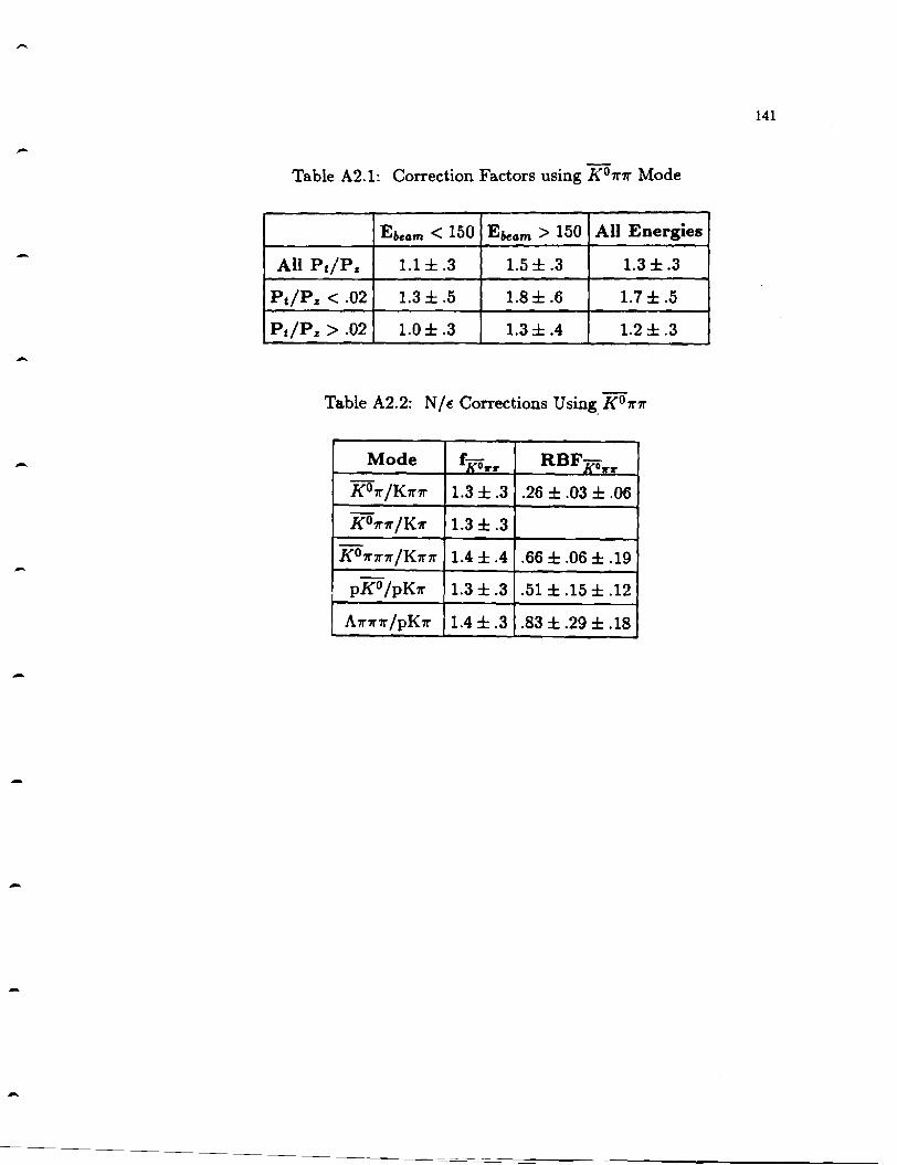
141
Table A2.l: Correction Factors using K 07r7r Mode
Ebeom < 150 Ebeam > 150 All Energies
All Pt/Pz 1.1 ± .3 1.5 ± .3 1.3 ± .3
Pt/Pz < .02 1.3 ± .5 1.8 ± .6 1.7 ± .5
Pt/Pz > .02 1.0 ± .3 1.3 ± .4 1.2 ± .3
Table A2.2: N/E Corrections Using_ K07r7r
Mode f-KOrr RBFK0n
K 0Tr/K7r7r 1.3 ± .3 .26 ± .03 ± .06
K 07r7r/K7r 1.3 ± .3
K 0 7r7r7r /K7r7r 1.4 ± .4 .66 ± .06 ± .19
pK0/pK7r 1.3 ± .3 .51 ± .15 ± .12
ATr7r7r /pK7r 1.4 ± .3 .83 ± .29 ± .18
-

142
charm signal with respect to Mark III is presented in table A2.1 as a function
of the beam energy and £&.(K.), where the entries in the table take the form· l'z '
f( E Pt (E.~ )) _ RBF(5;:)E691 beam' p a - •
11 RBF( KK~r)MIII (A2.l)
In table A2.2, the *(K.) dependent correction factors from table A2.1
(1.7 ± .5 for * < .02 : 1.2 ± .3 for * > .02) a.re applied to each of the
five charm modes, giving the overall corrections expressed in column 2, table
A2.2. These corrections are then applied to the uncorrected E691 branching
fractions (column 3, table Al.1) to give the corrected measurements in col-
umn 3, table A2.2. The variation in these overall correction factors illustrates
the mode to mode variation of the *(K.) distribution.
A3 The K* Study
It is interesting to consider the behaviour of the two decays K*0 -+
K-7r and K*+ -+ K 07r+ as a further check of this problem. The motiva-
tion for this portion of the study follows from a desire to understand the
systematic errors on these charm decay modes and, at the same time, to
generate corrections that are independent of the Mark III experiment. Such
corrections could even be applied to the K07r7r mode, which is sacrificed in
the previous method.
From isospin arguments, 1381 we know that the decay rates for K*0-+
K-7r+ and K*+ -+ Ko7r+ are the same, since they are 'strong' decays. We
assume the production of the charged and uncharged K*s is the same. At
-
-
-
-
-
-
-
-
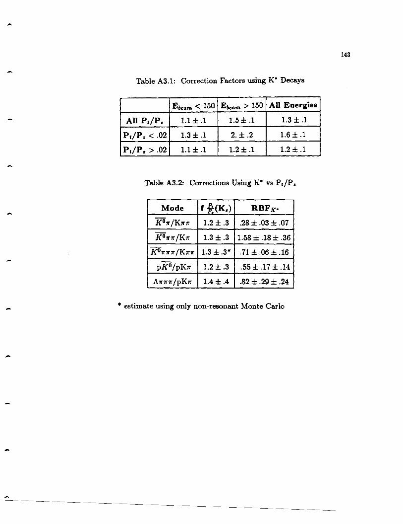
143
Table A3. l: Correction Factors using K• Decays
E6eam < 150 Ebeam > 150 All Energies
All Pt/Pz 1.1 ± .1 1.5 ± .1 1.3 ± .1
Pt/Pz < .02 1.3 ± .1 2.±.2 1.6 ± .1
Pt/P. > .02 1.1 ± .1 1.2 ± .1 1.2 ± .1
Table A3.2: Corrections Using K• vs P,/Pz
Mode f 9;(K,) RBFK·
K07r/K1nr 1.2 ± .3 .28 ± .03 ± .07
K 07r7r/K7r 1.3 ± .3 1.58 ± .18 ± .36
K 07r7r7r /K7r7r 1.3 ± .3* .71 ± .06 ± .16
pK0/pK7r 1.2 ± .3 .55±.17±.14
A7r7r7r /pK7r 1.4 ± .4 .82 ± .29 ± .24
- * estimate using only non-resonant Monte Carlo
-
-

144
this point then the number of acceptance corrected K•+s can be deduced
using the K•0-K-7r+ signal, and the Monte Carlo K~ efficiencies can be
tested . The correction factor obtained from this comparison is,
(A3.1)
where again the K• signals are split with respect to beam energy and lea.on
transverse momentum. The behaviour of the K•+ and K•0 signals with respect
to these parameters (and the NTRK and Ka momentum distributions) is
shown in figure A3.1. In this figure, the Monte Carlo plots are weighted with
respect to the data by the factor in equation A3.1 and, as before, figures
A3.l(B-D) include high beam energy events only(> 150 GeV /c2 ).
The agreement between the K 07r7r correction factors in table A2.1
and the K• corrections factors in table A3.l is good. This immediately
implies that any charm decay correction derived with the K•s will agree well
with that derived using the K 01r1r mode. Further, the correction for the
K01r1r mode itself, which we can't get using the other correction method,
will be nearly independent of 'RCK.) and of beam energy (and, in fact, kaon
momentum) 1$3
1 implying that the K. from the charged K• decays mimics the
K,, from the K 07r7r decay.
The relative branching fractions of all the meson and baryon charm
decay modes were calculated using the ~(K,,) dependent K• correction fac
tors (1.6 ± .1 for 9.- < .02 : 1.2 ± .1 for * > .02) and are listed in table
-
-
-

-
-
-
-
145
9 (A) 7 (8) 8 :+ 7 + 6 + Doto
I M.C. 6 s ·r-
- -+- -+-"' s 4 0 I I I -·- -·- -·- I -; 4 I
ri. I I 3 .,.
* -3 (/) 2 .... 2 z -·-la.I I -·-~o o
0-115115-150150-185 >185GtVI 0 20 40 60 80 100 _J EBEAM c2 Pt./R. <Ks) <(
z 7 7
<:> (Cl (0)
(/) 6 + 6 + II..
05 5 I
0 --·-- -+-Z4 + 4
3 3 I -;-
2 + 2 ~ I -·-I I •T• - ----·-0 0
0 4 8 12 16 20 24 28 0-15 15-25 25-40 >40Ge~ NTRK P(Ks) c2
FIGURE A3.1. For the decay mode K•+ -+ K 0 1r'+. The behaviour of the data and Monte Carlo K• events with respect to beam energy is shown in (A). The Monte Carlo plot is weighted by the factor in equation A3.l to give a idea of the beam dependence of the Monte Carlo inefficiency. Figures (B-D) are restricted to high beam energy events> 150 GeV /c2 and illustrate the dependence of this inefficiency on (B) 9.-<K.), (C) the number of tracks (excluding spurious and K• decay tracks), (D) the momentum of the K,,.

146
A3.2. As was inferred above, there is good agreement between the corrected
relative branching fractions in column 3 of tables A2.2 and A3.2.
A4 Conclusions
The straightforward neutral efficiency correction of 1.3 ± 0.3 gener
ated from the K 0 trtr mode has terrific simplicity. On the downside, it implic
itly incorporates a measurement from another experiment (Mark III) into our
results and, as it must be applied to all the neutral decay modes, pretends to
correct decay modes that have quite different analyses and topologies. In this
study, I investigated neutral particle (K.,) behaviour with respect to beam
energy, K, transverse and total momentum, and the total number of tracks
in the event. The marked dependence of the neutral efficiency correction on
beam energy, and on the slope of the kaon with respect to the beam, ~(K,),
can be seen in figures A2.1 and A3.1.
Tables A2.1 and A3.1 quantify this dependence. A close comparison
of these tables testifies to the uniformity of the two methods of correction. It
is also apparent that the beam energy dependence of the inefficiency is closely
related to the ~(K,) dependence, which is more than likely the fundamental
dependence of the inefficiency. The 9.-(K,) correction factors alone were
chosen to generate the efficiency corrections for the charm decay modes.
After calculating the corrections for these modes (given in column 2
of table A3.2), we need to obtain an estimate of the systematic error intro
duced using this correction method. The errors on the K• corrections in table
A3.1 are statistical errors from the K• fits and substantially underestimate
...
-
-
-
-
-
-
-

-
-
-
-
-
147
the systematic error we must assign to the full correction. The errors actually
assigned a.re on the order of 20% and reflect the fact that the charm decays
generate a substantial number of K,s with high ~(K,) (> .02) and high
momentum(> 25 GeV /c2 ) while the K* decays do not. rs3J The corrections
applied to the portion of the charm signal with these characteristics therefore
have large errors and generate a large contribution to the systematic error.
Comparing the distributions in figures A2.1 and A3.l, we can see
that the K*+ decay mimics the K 07r7r decay quite well in K,, momentum
and ~(Ks), and not so well with NTRK and beam energy. Efficiencies vary
slowly with respect to the number of tracks in the event, so the discrepancies
between the NTRK data plots should not contribute to the systematic error
greatly ( < 10%). (The fact that the Monte Carlo NTRK distribution for the
K*+ doesn't match its data distribution won't affect the K* corrections since
the K*0 exhibits similia.r behaviour). The error introduced by the discrepancy
in the beam energy distributions can be estimated from figures A2.l(a) and
A3.l(a) and is also of small effect ( < 10%).
Finally, the assumption that the production of the K*+ and the K*0 is
the same introduces a contribution to the systematic error of ,..., 10%. Studies
done on the K*s in experiment E516, the predecessor of experiment E691,
indicated that the relative production of K*o to K•+ was the same to within
,..., 10%. cs•J Results from kaon/proton interaction experimentsrss,ssJ and e+e
experiments1sr.saJ give similia.r limits. Combining these three contributions
to the systematic error with the 20% errors on the corrections themselves, we
obtain the systematic errors expressed in table A3.2. The systematic errors
148
reported in this appendix are due solely to the neutral efficiency corrections,
while the final errors are reported in chapter 7.
-
-
-
-
-
-
-
-
Recommended


![Possible Molecular States Composed of Doubly Charmed Baryons with Couple-channel … · 2019. 6. 13. · K ˇ+ˇ mass spectrum [46]. As an important member in the baryon family, there](https://img.pdfslide.us/doc/110x75/60c847809bfa720de13108f4/possible-molecular-states-composed-of-doubly-charmed-baryons-with-couple-channel.jpg)