Ph. D. DISSERTATION / TESIS DOCTORAL
Author:
Enrique Pérez Sánchez-Cañete
Characterization of CO2 exchanges in deep soils and caves and their role in the
net ecosystem carbon balance.
Promoters:
Francisco Domingo Poveda Andrew S. Kowalski
Penélope Serrano Ortíz
Universidad de Granada Mayo 2013 Programa de Doctorado Ciencias de la Tierra

Ph. D. DISSERTATION / TESIS DOCTORAL
Author
Enrique Pérez Sánchez-Cañete
Characterization of CO2 exchanges in deep soils and caves and their role in the
net ecosystem carbon balance
Programa de Doctorado Ciencias de la Tierra
Universidad de Granada Consejo Superior de Investigaciones Científicas
Grupo Física de la Atmósfera Centro Andaluz de Medio Ambiente

Tesis Doctoral
Characterization of CO2 exchanges in deep soils and caves and their role in the
net ecosystem carbon balance
Trabajo de investigación presentado por Enrique Pérez Sánchez-Cañete
para aspirar al grado de Doctor por la Universidad de Granada.
Esta Tesis Doctoral ha sido dirigida y supervisada por:
Dr. Francisco Domingo Poveda, Dr. Andrew S. Kowalski y
Dra. Penélope Serrano Ortíz
Mayo 2013

La Tesis doctoral que se expone en la siguiente memoria, titulada:
“Characterization of CO2 exchanges in deep soils and caves and their role in
the net ecosystem carbon balance” ha sido realizada por Enrique Pérez
Sánchez-Cañete para aspirar al grado de Doctor por la Universidad de
Granada. Se ha realizado conjuntamente en el Departamento de
Desertificación y Geoecología de la Estación Experimental de Zonas Áridas
(CSIC) y el Departamento de Física Aplicada de la Universidad de Granada.
La realización de esta Tesis ha sido financiada por una beca predoctoral de la
Junta de Andalucía, enmarcada dentro del proyecto de Excelencia titulado
“Balance de carbono en ecosistemas carbonatados: discriminación entre
procesos bióticos y abióticos (GEOCARBO, RNM-3721) financiado por la
Consejería de Innovación, Ciencia y Empresa de la Junta de Andalucía,
incluyendo fondos European Regional Development Fund (ERDF) y
European Social Fund (ESF) de la Unión Europea. El trabajo también ha sido
financiado parcialmente por proyectos del Ministerio Español de Ciencia e
Innovación, Carbored-II (CGL2010-22193-C04-02), SOILPROF (CGL2011-
15276-E), CARBORAD (CGL2011-27493), por las acciones integradas (PRI-
AIBDE-2011-0824 y HF2008-0057) y también por el Proyecto Europeo de
Séptimo Programa Marco (GHG Europe; Call FP7-ENV-2009-1.1.3.1; Project
Code 244122).

Como Directores de la Tesis confirmamos que el trabajo ha sido
realizado por el doctorando bajo nuestra dirección respetándose los derechos
de otros autores citados. Así mismo, el trabajo reúne todos los requisitos de
contenido, teóricos y metodológicos para ser admitido a trámite, a su lectura y
defensa pública, con el fin de obtener el referido Título de Doctor, y por lo
tanto AUTORIZAMOS la presentación de la referida Tesis para su defensa.
Directores de la Tesis
Fdo.:F. Domingo Poveda Fdo.:A.S. Kowalski Fdo.: P. Serrano Ortíz
Aspirante a grado de Doctor:
Fdo.: Enrique Pérez Sánchez-Cañete
Granada, Mayo de 2013

xi
Abstract
This Thesis arises to response to the anomalous CO2 fluxes detected
by the Eddy towers located on two carbonate and semiarid sites in the south-
east of Spain. In the soil-atmosphere CO2 exchanges in both El Llano de los
Juanes in the Sierra de Gádor and also Balsa Blanca located in the Natural
Park of Cabo de Gata-Nijar (Almeria province), significant CO2 emissions to
the atmosphere were detected. These emissions could only come from the soil
and not from the vegetation, occurring as they did mainly during the summer,
with senescent vegetation. For this reason, this Thesis focuses on monitoring
and characterization of the soil, distinguishing which are the main factors
implicated in CO2 exchanges with the atmosphere.
For the characterization and monitoring of subterranean CO2 soil CO2
profiles were established in both experimental sites with sensors installed at
three different depths (0.15, 0.5 and 1.5 m). Furthermore, in El Llano de los
Juanes sensors were installed at 0.25 m depth and in a borehole of 7 m depth,
which was sealed from the surface to simulate a karst cave.
With the first CO2 data obtained from the borehole, we realized that
the deep soil could store large amounts of CO2, because in the first 7 meters
we recorded values of up to 18000 ppm. Since we were interested in
determining the factors involved in CO2 ventilation from soils and
particularly in karstic areas containing numerous cavities, we launched an
examination of the literature regarding cave ventilation. This review triggered
the first publication of this Thesis (Chapter 1), because we realized that to
determine the buoyancy of air masses inside and outside the cave, and
therefore its ventilation, scientists were treating both air masses as if they had
equal composition. However, both our measurements in the borehole and
many others scientists working in other places had found great concentrations
xii
of CO2 in soil air, demonstrating a clear difference between the compositions
of soil and atmospheric air. These realizations led us to develop formulas to
correctly determine the virtual temperature and hence buoyancy of the air
masses considering the weight of CO2 in the composition of both air masses.
In Chapter 2 of this thesis, we applied the formulas previously
developed for 14 caves and holes around the world. We demonstrate the
significant errors that occur when predicting cave ventilation if not taking into
account the effect of CO2 air composition. To clarify the calculation tasks, we
provided an on-line tool to calculate the virtual temperature from input data
comprised of CO2, air temperature and relative humidity.
Having clarified the determination of ventilation between caves and
atmosphere, it was necessary to characterize and monitor the main factors
involved in soil ventilation and consequent CO2 emissions to the atmosphere.
From these measurements arose the publications corresponding to chapters 3
and 4 of this thesis.
In Chapter 3, is shown that in El Llano de los Juanes significant
decreases occur in the CO2 molar fraction of both soil (25 cm) and borehole
(7 m) when the wind is strong, as represented a high friction velocity. These
decreases in the CO2 molar fraction involve CO2 emissions to the atmosphere
which are detected by the Eddy Covariance tower. Also, was observed that on
days with light winds (calm), CO2 accumulated in the soil, whereas during
windy days large quantities of CO2 were emitted to the atmosphere.
Chapter 4 presents observations from the vertical CO2 profile located
in Balsa Blanca, with significant variations in the underground CO2 molar
fraction in just a few hours. These variations can result in an increase or
decrease of 400% compared with previous values. It is observed that changes
in the molar fraction are due to changes in atmospheric pressure. There are
two patterns in the subterranean CO2 fluctuations, one daily with two cycles
per day due to atmospheric tides and another cycle repeating every 3-4 days

xiii
(atmospheric synoptic scale) due to transitions between low and high pressure
systems. Also we observed that synoptic-scale pressure changes can affect the
CO2 fluxes detected by an eddy covariance tower. On days with rising
pressure, the downward CO2 flux is higher than on days with falling pressure
because on these days CO2 respired by plants tends accumulates in the soil.

xiv
xv
Resumen
Esta tesis surge para dar respuesta a los flujos de CO2 "anómalos"
detectados por las torres de Eddy Covariance situadas en dos sitios
carbonatados y semiáridos del Sureste español. En los intercambios de CO2
suelo-atmósfera, tanto en el Llano de los Juanes en la Sierra de Gádor como
en Balsa Blanca situada en el Parque Natural de Cabo de Gata-Níjar
(provincia de Almería), se detectaron importantes emisiones de CO2 a la
atmósfera. Estas emisiones sólo podían provenir del suelo y no de la
vegetación ya que ocurrían principalmente durante el verano, cuando la
vegetación está senescente. Además, se observó que dichas emisiones
"anómalas" llegaban a dominar los procesos de intercambio de CO2 entre la
atmósfera y la superficie contribuyendo notablemente en el balance anual de
carbono de estos ecosistemas. Por este motivo, esta tesis se ha centrado en la
monitorización y caracterización del CO2 del suelo, estudiando los principales
factores que intervienen en los intercambios de CO2 con la atmósfera.
Para la caracterización y monitorización del CO2 en el suelo se han
instalado en los dos sitios experimentales dos perfiles de CO2 con sensores a
tres profundidades (0.15, 0.5 y 1.5 m). Además, en el Llano de los Juanes
también se instaló un sensor a 0.25 m y se realizó una perforación de 7 m de
profundidad que posteriormente fue sellada en superficie para simular una
cavidad kárstica.
Con los primeros datos de fracción molar de CO2 obtenidos en la
perforación, nos dimos cuenta que el suelo en profundidad podía almacenar
enormes cantidades de CO2, ya que en los 7 primeros metros se llegaron a
registrar valores de 18000 ppm. Dado que nos interesaba conocer los factores
implicados en la ventilación del CO2 del suelo y sus cavidades, el doctorando
inició un trabajo de búsqueda bibliográfica sobre los aspectos relacionados
xvi
con la ventilación en cuevas. Esta revisión desencadenó la primera
publicación de esta tesis (Capítulo 1) al comprobar que para determinar la
flotabilidad de las masas de aire del interior y exterior de la cueva, y por tanto
su ventilación, los artículos ya publicados consideraban ambas masas de aire
con igual composición. Esta suposición era incorrecta en la gran mayoría de
los casos donde las elevadas concentraciones de CO2 en suelo marcaban una
clara diferenciación en la composición del aire del suelo y la atmósfera. Todo
esto nos llevó a proponer una nueva forma de calcular correctamente la
flotabilidad de las masas de aire teniendo en cuenta el CO2 en la composición
de ambas masas de aire.
En el Capítulo 2 de esta tesis, se aplicaron las ecuaciones
desarrolladas en el capítulo anterior en 14 cuevas y perforaciones de todo el
mundo, demostrando los importantes errores que se cometen a la hora de
interpretar la ventilación de las cuevas cuando no es tenido en cuenta el efecto
del CO2 en la composición del aire. Para facilitar las labores de cálculo, se
ofrece gratuitamente y de forma “online” la metodología necesaria para su
cálculo de una manera muy simple en la que sólo es necesario aportar los
datos de CO2, temperatura del aire y humedad relativa. Una vez conocida la
forma de determinar la ventilación entre las cavidades y la atmósfera, se
procedió a caracterizar y monitorizar los principales factores implicados en la
ventilación del suelo y las emisiones a la atmósfera. Fruto de este estudio se
publicaron una serie de artículos científicos que dan origen a los Capítulos 3 y
4 de esta tesis.
El Capítulo 3 se centra en el Llano de los Juanes y concluye que el
viento es el principal factor responsable de las emisiones de CO2 en épocas de
sequía. En este ecosistema se midieron importantes descensos en la fracción
molar tanto del suelo (0.25 m) como de la perforación (7 m) con fuertes
vientos y por lo tanto alta velocidad de fricción (>0.3 m s-2). Estos descensos
en la fracción molar del CO2 implican emisiones de CO2 hacia la atmósfera
que se ven reflejados en la torre Eddy Covariance. De este modo, en días
xvii
ventosos el CO2 almacenado en el suelo durante los días de calma es emitido
a la atmósfera.
El Capítulo 4, centrado en Balsa Blanca, demuestra que en este
ecosistema los cambios en la fracción molar de CO2 se deben a cambios en la
presión atmosférica. En el perfil vertical de CO2 situado en Balsa Blanca, se
registran importantes variaciones en la fracción molar de CO2 en tan sólo
unas horas. Estas variaciones pueden suponer un incremento o descenso de un
400% respecto a sus valores anteriores. En este sentido, de diferencian dos
patrones en las fluctuaciones del CO2 subterráneo, uno a escala diaria con dos
ciclos por día debidos a las mareas atmosféricas y otro a escala sinóptica (3-4
días) debido a la transición entre bajas (borrasca) y altas presiones
(anticiclón). También se ha observado como a escala sinóptica los cambios de
presión pueden afectar a los flujos de CO2 detectados por la torre Eddy
Covariance. En días con incrementos en la presión atmosférica se produce
mayor fijación de CO2 que en días con menor presión en los que el CO2
respirado por las plantas tiende a acumularse en el suelo.

xviii
xix
Acknowledgements
Una vez terminada la redacción de la parte más científica de la tesis,
ahora me centraré en una de las partes que más deseaba escribir. Esta parte
en la que agradezco todo el apoyo recibido durante estos maravillosos años
dedicados a labores investigadoras.
Quiero agradecer la importante labor que han realizado mis
directores, Francisco Domingo, Andrew S. Kowalski y Penélope Serrano-Ortiz
en mi formación predoctoral. A Paco le agradezco enormemente su profunda
confianza en mí trabajo, siempre con respuestas optimistas y de apoyo. A
Andy quisiera agradecerle por haber apostado por mí, en un primer
momento como técnico y posteriormente como predoctoral. Si no es por él
no me habría planteado hacer el doctorado. Gracias por haber pasado
tantísimas horas respondiendo mis dudas y guiándome por el camino
correcto. A Penélope que voy a decir de ella…, es perfecta como directora de
tesis y maravillosa como compañera de trabajo. Siempre ha estado a mi lado
para resolver mis dudas al instante y ha sido una perfecta asesora para decir
que es importante y que no lo es y a que hay que dedicarle más o menos
tiempo.
Quiero también agradecer el apoyo que he recibido por mis
compañeros de trabajo. Oscar, gracias por haberte unido a nuestro grupo de
investigación. Eres un estupendo compañero tanto dentro del trabajo como
fuera de él. Borja, gracias por todos los buenos momentos que pasamos en la
facultad y por todo lo que me ayudaste en la parte física y de cálculos con los
distintos programas durante mis inicios en la beca. Ana, gracias por hacerme
compañía en la Facultad y por sonreír siempre, mucha suerte en el futuro.
xx
A mis compañeros tanto de la Facultad de Ciencias como del CEAMA
quiero agradecerles por haberse comportado como verdaderos amigos y
ayudarme siempre que le he solicitado algo. A Dani Argúeso, Jose, Dani
Calandria, Maria, Samir y Reiner quería agradeceros todas las horas que
hemos pasado juntos contándonos nuestras alegrías y nuestros penas, las
largas charlas de política, futbol, jefes… Quisiera agradecer también a todos
mis compañeros del CEAMA por alegrarme casi todos los viernes del año,
algún que otro día entre semana, algún que otro fin de semana y por las
numerosas barbacoas. A Hassan, Juan Antonio, Antonio, María José, Alberto,
Lucas, Paco Pepe, Inma Alados, Inma Foyo, Jesús, Juanlu, Fran, Gloria, Dani,
Manuel y Jaime, gracias por vuestra amistad y estupendo ambiente de
trabajo.
También quiero agradecer esta tesis a Juan Lorite, ya que él fue el
que me introdujo en la investigación. Gracias por dejarme acompañarte en la
busqueda de flora amenazada en Sierra Nevada y recomendarme a Jorge
Castro para trabajar junto a ambos. Gracias también a Jorge por haberme
contratado para trabajar con él, y por su trato tan cercano y amable.
Agradezco también a Sara, Ángela, Inma, Ramón y Susana por haber
trabajado codo a codo, día tras día en Sierra Nevada y pasar formidables
momentos.
Quiero agradecer también a Jukka Pumpanen, por haberme
aceptado y tratado perfectamente en mi primera estancia. También quiero
agradecer a Russ Scott por haberme tratado estupendamente en mi estancia
en Arizona, es un investigador estupendo y un compañero formidable, que
me hizo sentir parte de su familia.
También quiero agradecer a Cecilio su enorme apoyo en las labores
de campo, siempre dispuesto a echar una mano. A Arnaud por las
xxi
interesantísimas conversaciones sobre instrumentación que hemos tenido, y
por saber todas las respuesta a las preguntas que te he realizado. A mis
compañeras Laura y Olga por la ayudarme tantísimas veces en la recogida de
datos.
Por último quiero agradecer y dedicarle personalmente esta tesis a
mi MADRE y a mi PADRE, los escribo con mayúscula porque se lo merecen.
Mama, tu sabes que si no es por ti, por tu coraje y por luchar moviendo cielo
y tierra para mi educación no estaría aquí ahora mismo. Papa también quiero
recordarte que entré en la carrera porque me dijiste, “la vida de estudiante
es muy bonita, prueba un año y si no te gusta te vas” y aquí me ves. María y
Elena siempre habéis estado ahí para ayudarme con todo, estoy muy
orgulloso de vosotras. También quiero dedicársela a mis abuelos, Itas,
Miguel, Juan de Dios y Antonia sé que están orgullosos de su nieto. Mari,
gracias por estar a mi lado durante todos estos maravillosos años, sólo te
diré que “la constancia hace el triunfo”, el 2013 es nuestro año.

Table of contents
Abstract .................................................................................................. xi
Resumen ................................................................................................. xv
Acknowledgements ................................................................................ xix
Table of contents ....................................................................................... .
1. Background: The global carbon Cycle ..................................................... 1
1.1. Societal concern ............................................................................... 1
1.2. Definition of the Global Carbon Cycle .............................................. 2
1.3. CO2 exchange measurements at ecosystem level ............................ 5
1.4. Other processes involved in C sequestration and loss apart from concurrent biological activity ....................................................................... 6
1.5. Subterranean CO2 ............................................................................ 7
1.6. Objectives and outline of the thesis .................................................. 9
2. Fundamentals ................................................................................. 11
2.1. Measuring CO2 in air ...................................................................... 11
2.2. Eddy covariance flux measurements ............................................. 12
3. Experimental Field Sites .................................................................. 15
3.1 El Llano de los Juanes ..................................................................... 15
3.2 Balsa Blanca .................................................................................... 19
4. Results ............................................................................................ 31
4.1 Chapter 1 ........................................................................................ 33
A New Definition of the Virtual Temperature, Valid for the Atmosphere and the CO2-Rich Air of the Vadose Zone .................................................. 33
4.2 Chapter 2 ........................................................................................ 45
Cave ventilation is influenced by variations in the CO2-dependent virtual temperature ............................................................................................... 45
4.3 Chapter 3 ........................................................................................ 73
Subterranean CO2 ventilation and its role in the net ecosystem carbon balance of a karstic shrubland ................................................................... 73
4.4 Chapter 4 ........................................................................................ 87
Deep CO2 soil inhalation/exhalation induced by synoptic pressure changes and atmospheric tides in a carbonated semiarid steppe ........................... 87
5. General discussion and conclusions ............................................... 113
5.1 General discussion ............................................................................. 113
State of the art Subterranean CO2 ....................................................... 113
Recent relevant publications ................................................................ 115
Perspectives on future research .......................................................... 116
5.2 Conclusions......................................................................................... 117
5.3 Conclusiones....................................................................................... 119
List of abbreviations ............................................................................. 127
List of symbols ...................................................................................... 129
Curriculum Vitae of Enrique Pérez Sánchez-Cañete ................................ 131
Publications .............................................................................................. 131
Journal papers ...................................................................................... 131
Book Chapters ...................................................................................... 133
International Conference Contributions .............................................. 133

1. Background: The global carbon Cycle
1
1. Background: The global carbon Cycle
The global carbon cycle in the atmosphere can be described simply as
the sum of CO2 inputs less outputs. Today's society and the way it interacts
with the environment is causing a constant increase in the atmosphere CO2
content, mainly due to the burning of fossil fuels and changes in land use.
This increase in atmospheric CO2 leads to increase of mean earth temperature,
causing numerous feedbacks with the different ecosystems which deserve a
better understanding through research.
1.1. Societal concern
During the last five decades a great number of scientists have worked
to characterize accurately the role of the different terrestrial subsystems
(biosphere, lithosphere, hydrosphere and atmosphere) in the global carbon
cycle. The importance of characterizing the global carbon cycle and the
factors involved is highlighted by the progressive increase in the atmospheric
CO2 molar fraction [Keeling, 1960]. Thus, in 1972 the Stockholm Conference
was organized, being the first conference convened by the United Nations
(UN) considering the need for a common outlook and principles to inspire and
guide the peoples of the world in the preservation and enhancement of the
human environment.
With growing concern over the increase in greenhouse gases (GHGs)
and diverse environmental problem, the UN held a summit in Rio de Janeiro
in 1992, known as the Earth Summit. At this summit an international
environmental treaty was approved known as the United Nations Framework
Convention on Climate Change (UNFCCC), with the objective of stabilizing
greenhouse gas (GHG) concentrations in the atmosphere at a level that would
prevent dangerous anthropogenic interference with the climate system. Also,
this stabilization was targeted for a timeframe that would allow ecosystems to
CO2 exchanges in deep soils and caves and their role in the NEBC
2
adapt naturally to climate change, ensuring that food production not be
threatened and allowing economic development to proceed in a sustainable
way.
Later, after the signing of Kyoto Protocol in 1997, the need to reduce
emissions of GHGs in net terms was affirmed, taking into account not only
the total production of contaminating gases, but also the uptake capacity of
such contaminants in each country. For this reason some countries chose to
reduce their net emissions by increasing carbon sequestration by forests. In
2001 at the Seventh UN Conference on Climate Change held in Marrakech
the legal aspects of the Kyoto Protocol were established and treated
fundamental issues such as the development of methods to estimate, measure
and monitor changes in carbon emitted or stored by the different sources and
sinks.
For these reasons, it is essential to develop methodologies for the
accounting of anthropogenic emissions by sources and/or anthropogenic
removals by sinks. In this context, technological advancement has improved
the quality of micro-meteorological information and thus understanding of
CO2 exchanges between the atmosphere and land surface. These
advancements are generating much information on spatial scales from small
(leaf, plant and soil) to large (ecosystem, regional and global).
1.2. Definition of the Global Carbon Cycle
The global carbon cycle depends on feedbacks among a number
of source and sink processes occurring among different systems (reservoirs or
pools): ocean, atmosphere, lithosphere and biosphere (Fig. 1). Between these
reservoirs, carbon moves at various natural rates of exchange (fluxes). These
exchange processes operate at different time scales: from seconds
(photosynthesis) to millennia (formation of fossil fuels) modifying the C
composition of reservoirs [Boucot and Gray, 2001]. While CO2 represents
1. Background: The global carbon Cycle
3
only 0.039% of the atmosphere (molar fraction) and the atmosphere is a small
carbon reservoir, CO2 plays two vital roles for life on earth. 1) It is involved
in the modification the energy balance of our planet because it is one of the
principal gases involved in the greenhouse effect [IPCC 2007], absorbing
infrared radiation from earth surface and reemitting part of that energy back
towards the surface to increasing the average surface temperature. 2) Plants
grow through photosynthesis, taking up CO2, which is later emitted to
atmosphere through respiration by plants, animals and microorganisms.
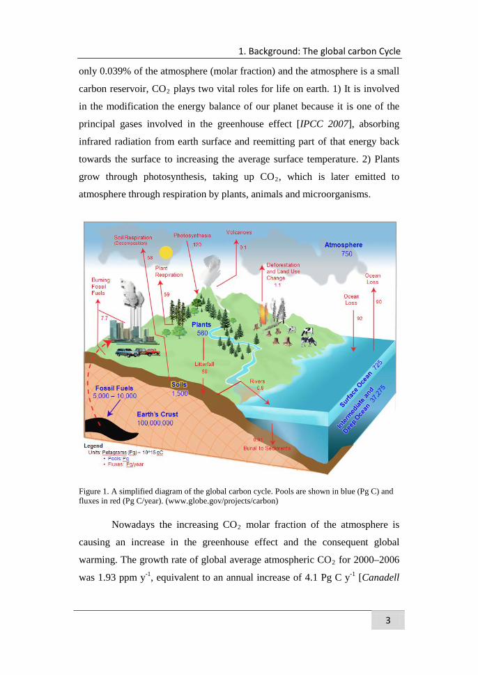
Figure 1. A simplified diagram of the global carbon cycle. Pools are shown in blue (Pg C) and fluxes in red (Pg C/year). (www.globe.gov/projects/carbon)
Nowadays the increasing CO2 molar fraction of the atmosphere is
causing an increase in the greenhouse effect and the consequent global
warming. The growth rate of global average atmospheric CO2 for 2000–2006
was 1.93 ppm y-1, equivalent to an annual increase of 4.1 Pg C y-1 [Canadell
CO2 exchanges in deep soils and caves and their role in the NEBC
4
et al., 2007]. This occurs because there is an imbalance between sources
(Fossil fuel and respiratory emissions) and sinks (photosynthesis).
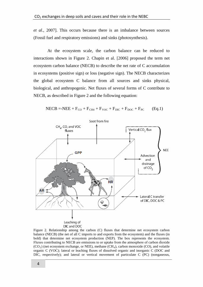
At the ecosystem scale, the carbon balance can be reduced to
interactions shown in Figure 2. Chapin et al. [2006] proposed the term net
ecosystem carbon balance (NECB) to describe the net rate of C accumulation
in ecosystems (positive sign) or loss (negative sign). The NECB characterizes
the global ecosystem C balance from all sources and sinks physical,
biological, and anthropogenic. Net fluxes of several forms of C contribute to
NECB, as described in Figure 2 and the following equation:
NECB =-NEE + FCO + FCH4 + FVOC + FDIC + FDOC + FPC (Eq.1)
Figure 2. Relationship among the carbon (C) fluxes that determine net ecosystem carbon balance (NECB) (the net of all C imports to and exports from the ecosystem) and the fluxes (in bold) that determine net ecosystem production (NEP). The box represents the ecosystem. Fluxes contributing to NECB are emissions to or uptake from the atmosphere of carbon dioxide (CO2) (net ecosystem exchange, or NEE), methane (CH4), carbon monoxide (CO), and volatile organic C (VOC); lateral or leaching fluxes of dissolved organic and inorganic C (DOC and DIC, respectively); and lateral or vertical movement of particulate C (PC) (nongaseous,
1. Background: The global carbon Cycle
5
nondissolved) by processes such as animal movement, soot emission during fires, water and wind deposition and erosion, and anthropogenic transport or harvest. Fluxes contributing to NEP are gross primary production (GPP), autotrophic respiration (AR), and heterotrophic respiration (HR), [Chapin et al., 2006].
1.3. CO2 exchange measurements at ecosystem level
The study of CO2 exchanges between the atmosphere and Earth's
surface began in the 1980s with a few pilot studies, which were extended to
regional networks in the 1990s. Today these studies have been extended to
more than 500 locations where carbon exchange is measured in different
ecosystems. To measure these exchange the eddy covariance technique (EC)
is used. This technique is being applied in the main ecosystems: forests
[Carrara et al., 2004; Valentini et al., 2000], crops [Anthoni et al., 2004;
Aubinet et al., 2009], deserts [Hasting et al., 2005; Wohlfahrt et al., 2008] and
shrublands [Reverter et al., 2010; Scott et al., 2012; Serrano-Ortiz et al.,
2009]. Furthermore this technique is used to evaluate the effects of
disturbances like fire [Amiro et al., 2003; Serrano-Ortiz et al., 2011] or
harvest [Kowalski et al., 2003; Kowalski et al., 2004].
The eddy covariance technique is used by the international network of
flux towers "FLUXNET" (at present over 500 tower sites) to measure the
exchanges of CO2, water vapor, and energy between ecosystems and the
atmosphere. FLUXNET is an integrated network of regional networks
including Ameriflux from the Americas, AsiaFlux from Asia-Japan, OzNet
from Oceania and Carboeurope from Europe, and each of these regional
networks include networks of different countries. Concretely in Spain there is
a systematic observation network of carbon and energy flows in terrestrial
ecosystems called CARBORED-ES. The programs proposed by these
networks interpret CO2 fluxes as resulting directly from concurrent biological
(photosynthetic or respiratory) activity [Baldocchi, 2003; Falge et al., 2002;
Houghton, 2002; Reichstein et al., 2005].
CO2 exchanges in deep soils and caves and their role in the NEBC
6
1.4. Other processes involved in C sequestration and loss apart from concurrent biological activity
The non-biological processes that can contribute in the net ecosystem
carbon balance (NEBC) are the following [Serrano-Ortiz et al., 2012]:
• Weathering processes, mainly by carbonates rocks.
Weathering releases CO2 during precipitation; however
during dissolution atmospheric CO2 is consumed [Plummer et
al., 1979].
• Biomineralization processes. Fungi, lichens and cyanobacteria
can modify calcite dissolution or precipitation, taking up or
emitting CO2 [Verrecchia et al., 1990].
• Erosion processes. Transport of particles by air or water can
decrease or increase the soil organic carbon in a soil [Boix-
Fayos et al., 2009; Jacinthe and Lal, 2001].
• Photodegradation processes. These occur mainly in dry
ecosystems when the ultraviolet light provokes a direct
breakdown of organic matter to CO2 [Brandt et al., 2009].
• Ventilation processes. The wind penetrates into subsoil
(cracks, pores and cavities) causing emission of previously
stored CO2. A large part of this thesis focuses on this topic,
which is a novel line of research largely neglected by the
FUXNET community.
The programs proposed by this network interpret CO2 fluxes as
resulting from concurrent biological (photosynthetic or respiratory) activity
[Baldocchi, 2003; Falge et al., 2002; Houghton, 2002; Reichstein et al.,
2005], neglecting CO2 exchanges due to, as they shall be termed here,
“alternative” processes. The emergence of studies focusing on alternative CO2
exchanges dates from less than a decade. Emmerich [2003] attributed the CO2
1. Background: The global carbon Cycle
7
emitted after rain events following prolonged drought periods to carbonate
dissolution in the soil. Mielnick et al. [2005] found large positive CO2
effluxes in the summer that could be attributing to increased soil abiotic
sources of CO2. However, it was not until 2008 that the first clear evidence of
alternative influences on net CO2 exchange was detected by eddy covariance
[Kowalski et al., 2008].
Kowalski et al. [2008] found periods in which CO2 exchanges could
not be interpreted purely in terms of concurrent biological processes, but these
should be explained by alternative processes. These alternative CO2
contributions were detected in two carbonated experimental sites, one in the
north of Spain (Altamira Cave) and the other in the South (Sierra de Gádor).
At this last experimental site, Serrano-Ortiz et al. [2009] confirmed that
during the whole study period from 2004 to 2007, episodes of alternative CO2
fluxes were detected during dry season. These papers highlighted the
important need to characterize the processes of subterranean ventilation and
dissolution/precipitation of carbonates for the correct estimate of CO2 fluxes
exchanged by carbonated ecosystems.
1.5. Subterranean CO2
Subterranean ventilation and CO2 dissolution/precipitation processes have
their greatest magnitudes in limestone and karst soils. Soils are a large pool of
terrestrial carbon (C), estimated to contain 1576 Pg C [Eswaran et al., 1993]
which is nearly three times higher than the amount of C in aboveground
biomass and double that of the atmosphere [Schlesinger, 1997]. A 10%
decrease of total soil organic carbon would be equivalent to the emitted
anthropogenic CO2 over 30 years [Kirschbaum, 2000]. At present the
outcropping of carbonate soils are extended on ca. 12-18% of the water-free
Earth [Ford and Williams, 1989]. These present an enormous capacity to store
large amounts of CO2 in subsurface cracks, pores and cavities, reaching
values that exceed 50000 ppm of CO2 (5% of air volume) both in caves
CO2 exchanges in deep soils and caves and their role in the NEBC
8
[Denis et al., 2005; Howarth and Stone, 1990] and in soil [Crowther, 1983;
Ek and Gewelt, 1985]. Later, through the venting of these subterranean spaces
the stored gaseous CO2 can be exchanged with the atmosphere.
Knowing the distribution of large cavities and fractures that can emit
CO2 to the atmosphere is vital to the interpretation of ecosystem CO2 fluxes
[Were et al., 2010]. Concretely, this study showed that two proximate EC
towers with different footprints (or areas of surface influence) agreed for CO2
measurements in periods when respiration and photosynthesis processes were
dominant (biological periods), however during periods dominated by
alternative processes (“abiotic periods”) agreement was not good. They
concluded that the disagreement between measurements was due to sub-
surface heterogeneity within the footprint.
Therefore it is necessary to study the behavior of subterranean CO2,
mainly over carbonate soils, to understand when such alternative CO2
exchanges are produced and so correctly interpret CO2 fluxes at the
ecosystem level for posterior modeling, helping to improve our overall
understanding of the global carbon cycle.
1. Background: The global carbon Cycle
9
1.6. Objectives and outline of the thesis
The main objective of this thesis is to improve the knowledge of
subterranean CO2 dynamics, distinguishing which are the drivers involved in
its transport and exchange with the atmosphere.
In the different chapters of this thesis, we will try to achieve the main
objective by meeting the specific objectives identified for each chapter:
- Study with precision the buoyancy of an underground air mass
depending of the CO2 content (Chapter 1).
- Examine the errors that can be committed in different caves around
the world when neglecting CO2 effects on air buoyancy and therefore
its potential for ventilation (Chapter 2).
- Know the role of subterranean CO2 ventilation in the net ecosystem
carbon balance of a subalpine shrubland (Chapter 3).
- Identify the role of synoptic and shorter-period barometric changes
(atmospheric tides) in subterranean CO2 variations within a soil
vertical profile of a low-altitude shrubland (Chapter 4).

CO2 exchanges in deep soils and caves and their role in the NEBC
10
Fundamentals
11
2. Fundamentals
2.1. Measuring CO2 in air
The results of this thesis are mainly generated by CO2 measurements
in air using different instruments and scenarios. In all cases, CO2 was
quantified through direct measurement of laser absorption by gaseous CO2 in
the air. Given a source with radiant power and a detector some distance away
through the gas, in the absence of reflection, absorptance (α) by gas i is
defined by the Beer–Bouguer- Lambert law as:
II i
ii0
11 −=−= τα (Eq. 2)
where τ i is transmittance through gas i, Ii is the intensity of the incident
radiation in the absorption band with some concentration of gas i present, and
I0 is the intensity of the radiation in the absorption band with zero
concentration of i present. Infrared gas analyzers (IRGAs) measure gases like
CO2 or H2O [McDermitt et al., 1994] by determining the absorption by:
01
AAi
i −=α (Eq. 3)
where Ai is the power received from the source in an absorbing wavelength
for gas i, and Aio is the power received from the source in a reference
wavelength that does not absorb gas i. The number density (n in mmol/m3) of
gas i can be determined by:
=
ei
iiieii P
SfPn α (Eq. 4)
CO2 exchanges in deep soils and caves and their role in the NEBC
12
Pressure is denoted as Pei because it is the equivalent pressure for the
gas i. Equivalent pressure is potentially different from total pressure P if there
are gases present other than i that affect how gas i absorbs radiation. The
calibration functions fi and Si are generated by measuring a range of known
densities. Since gas standards are not available in “known densities”, the ni
values are computed from a known molar fraction mi (moles of gas per mole
of air) using the ideal gas law:
RTPmn ii = (Eq. 5)
For gas i the mass density (g/m3) can be obtained by multiplying the
number density by its molecular weight Mi:
iiMi nMn = (Eq. 6)
Finally the molar fraction for the gas i ( iχ , μmol/mol) can be
obtained by:
PRTnMi
i =χ (Eq. 7)
where R is the universal gas constant and T the temperature.
2.2. Eddy covariance flux measurements
The eddy covariance technique is used for measure exchanges of heat,
mass, and momentum between a flat, horizontally homogeneous surface and
the overlying atmosphere. This technique is used by scientific community for
the measurement of the turbulent exchanges of CO2 and H2O between an
ecosystem and the atmosphere [Baldocchi et al., 2001]. Ecosystem exchanges,
defined by much of something moves per unit time through a unit area, are
Fundamentals
13
truly flux densities by nonetheless commonly termed “fluxes”. The main
equations involved in determining the CO2 fluxes are described below.
In atmospheric turbulence, any variable ξ is typically broken into two
parts in a process known as Reynolds decomposition:
ξξξ ′+= (Eq. 8)
representing the sum of a mean ξ and a fluctuation part ξ ′ . With the
application of equation 8 and Reynolds’ rules, the turbulent flux can be
written:
cd swF ′′= ρ (Eq. 9)
where ρd is the dry air density, w the vertical wind and sc the CO2 mixing
ratio.
Since the open path analyzers (Li-cor 7500) measure CO2 density
rather than mixing ratio, fluctuations in temperature and water vapor cause
fluctuations in CO2 and other trace gases that are not associated with the flux
of the trace gas of interest. Therefore, systematic corrections are required to
account for “density effects” (hereafter, WPL terms) [Webb et al., 1980].
Thus, the turbulent CO2 flux can be accurately determined by eddy covariance
from gas density fluctuations according to
( ) TwT
wwF cd
d
ccC ′′
++′′
+′′=
ρµσρρρµρ 1 (Eq. 10)
where FC is the final corrected CO2 flux, cw ρ′′ is the covariance between
vertical wind and CO2 density, μ is the ratio of molar masses of dry air and
Water flux term Heat flux term (water dilution) (termal expansión)
CO2 exchanges in deep soils and caves and their role in the NEBC
14
water vapor (1.6077, md/mv), ρc is CO2 density, ρd is dry air density, σ is the
ratio of density of water vapor and dry air (ρv /ρd), T is mean air temperature
in K and Tw ′′ is the covariance between vertical wind and temperature.
Another possible, related correction is due to sensor self-heating
[Burba et al., 2008]. Since the Li-Cor 7500 (open -path) IRGA actively heats
to maintain an operating temperature, this correction would be higher in cold
ecosystems [Reverter et al., 2010] than in warm ecosystem [Reverter et al.,
2011]. At present, there is no consensus regarding how or whether to apply
this correction, which would depend on wind speed, the inclination of the
sensor and incident solar radiation. In any event, the self-heating correction is
significant only when attempting long-term integrations, whereas its effect is
minimal when the focus is on process studies, as is the case in this thesis.
More details of eddy covariance flux measurement can be found in
specific books [Aubinet et al., 2012] or relevant theses [Reverter, 2011;
Serrano-Ortiz, 2008].
Experimental Field Sites
15
3. Experimental Field Sites
The studies presented in this thesis were conducted mainly in two
ecosystems situated in southeast Spain, one at high elevation (El Llano de los
Juanes, 1600 m) and the other close to sea level (Balsa Blanca, 200 m).
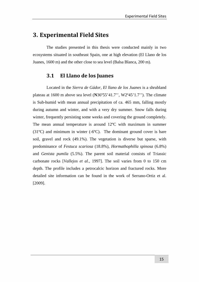
3.1 El Llano de los Juanes
Located in the Sierra de Gádor, El llano de los Juanes is a shrubland
plateau at 1600 m above sea level (N36º55’41.7’’, W2º45’1.7’’). The climate
is Sub-humid with mean annual precipitation of ca. 465 mm, falling mostly
during autumn and winter, and with a very dry summer. Snow falls during
winter, frequently persisting some weeks and covering the ground completely.
The mean annual temperature is around 12ºC with maximum in summer
(31ºC) and minimum in winter (-6ºC). The dominant ground cover is bare
soil, gravel and rock (49.1%). The vegetation is diverse but sparse, with
predominance of Festuca scariosa (18.8%), Hormathophilla spinosa (6.8%)
and Genista pumila (5.5%). The parent soil material consists of Triassic
carbonate rocks [Vallejos et al., 1997]. The soil varies from 0 to 150 cm
depth. The profile includes a petrocalcic horizon and fractured rocks. More
detailed site information can be found in the work of Serrano-Ortiz et al.
[2009].
CO2 exchanges in deep soils and caves and their role in the NEBC
16
Figure 3.El Llano de los Juanes, Sierra de Gádor. December of 2009
An eddy covariance system was installed in May of 2004, mounted on
a top of a 2.5 m micrometeorology tower. Densities of CO2 and water vapour
as well as barometric pressure were measured by an open-path infrared gas
analyser (IRGA Li-Cor 7500, Lincoln, NE, USA), calibrated monthly. Wind
speed and sonic temperature were measured by a three-axis sonic anemometer
(CSAT-3, Campbell Scientific, Logan, UT, USA; hereafter CSI). The friction
velocity (u*) is defined as the turbulent velocity scale resulting from square
root of the (density-normalized) momentum flux magnitude [Stull, 1988].
Temperature and relative humidity were measured by a thermohygrometer
(HMP45C, CSI). At 1.5 m above ground level there were two quantum
sensors (LI-190, Li-Cor) measuring incident and reflected photon fluxes, a net
radiometer (NR-Lite, Kipp&Zonnen, Netherlands) and a tipping-bucket rain
gauge (ARG100, CSI). Below ground there were two soil heat flux plates at 8
cm (HFP01, CSI), an averaging soil thermocouple probe (TCAV, CSI) and 3
water content reflectometers (CS616, CSI). A data-logger (CR3000, CSI)
managed the measurements data at 10 Hz and recording at the same frequency
Experimental Field Sites
17
only of the wind and IRGA data. The averages of the rest of the variables and
turbulent fluxes were computed every half-hour.
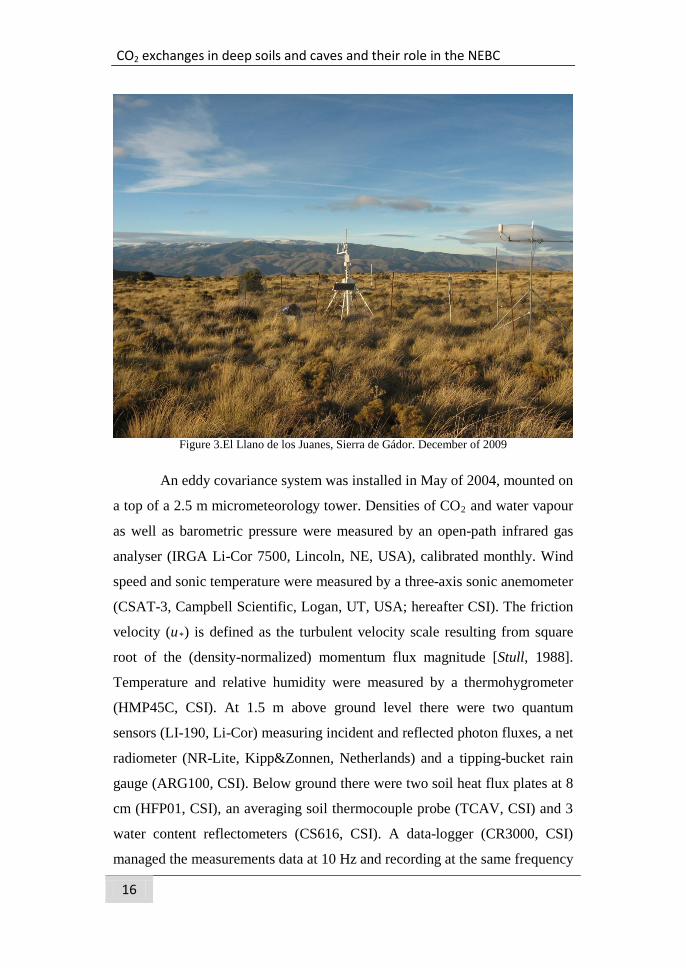
Forty meters northwest of the tower several instrumentation were
installed to measure different parameters associated with CO2 production in
subsoil. In June of 2009 two CO2 molar fraction sensors (GMP-343, Vaisala,
Inc., Finland; hereafter Vaisala) were installed in the soil and in a borehole
penetrating a bedrock outcropping. The CO2 soil sensor was installed
horizontally at 25 cm depth, together with a soil temperature probe (107
temperature probe, CSI) and a water content reflectometer (CS616, CSI).
Figure 4. Installing CO2 sensor, soil water content and temperature probe.
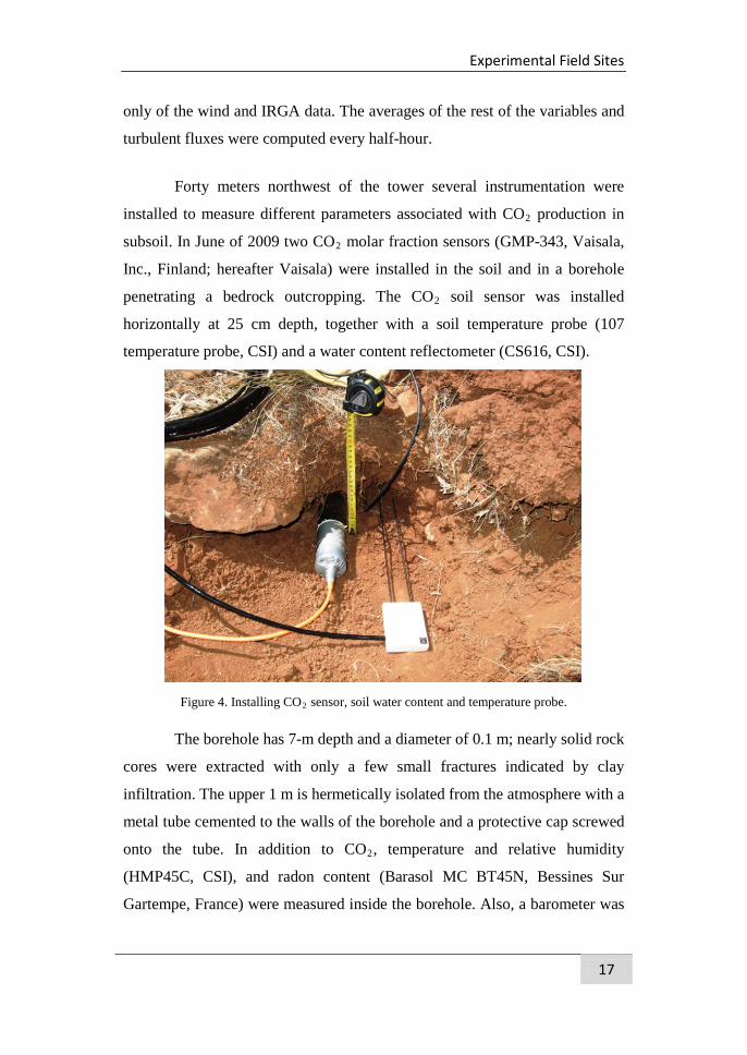
The borehole has 7-m depth and a diameter of 0.1 m; nearly solid rock
cores were extracted with only a few small fractures indicated by clay
infiltration. The upper 1 m is hermetically isolated from the atmosphere with a
metal tube cemented to the walls of the borehole and a protective cap screwed
onto the tube. In addition to CO2, temperature and relative humidity
(HMP45C, CSI), and radon content (Barasol MC BT45N, Bessines Sur
Gartempe, France) were measured inside the borehole. Also, a barometer was
CO2 exchanges in deep soils and caves and their role in the NEBC
18
installed at the soil level (PTB101B, Vaisala). Measurements were made
every 30s and stored as 5min averages by a data-logger (CR23X, CSI).
Figure 5. Left, doing the borehole in Llano de los Juanes. Right, rock cores.
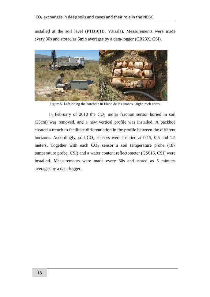
In February of 2010 the CO2 molar fraction sensor buried in soil
(25cm) was removed, and a new vertical profile was installed. A backhoe
created a trench to facilitate differentiation in the profile between the different
horizons. Accordingly, soil CO2 sensors were inserted at 0.15, 0.5 and 1.5
meters. Together with each CO2 sensor a soil temperature probe (107
temperature probe, CSI) and a water content reflectometer (CS616, CSI) were
installed. Measurements were made every 30s and stored as 5 minutes
averages by a data-logger.
Experimental Field Sites
19
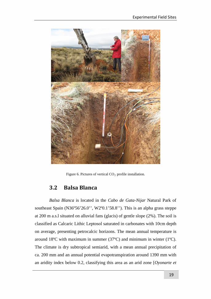
Figure 6. Pictures of vertical CO2 profile installation.
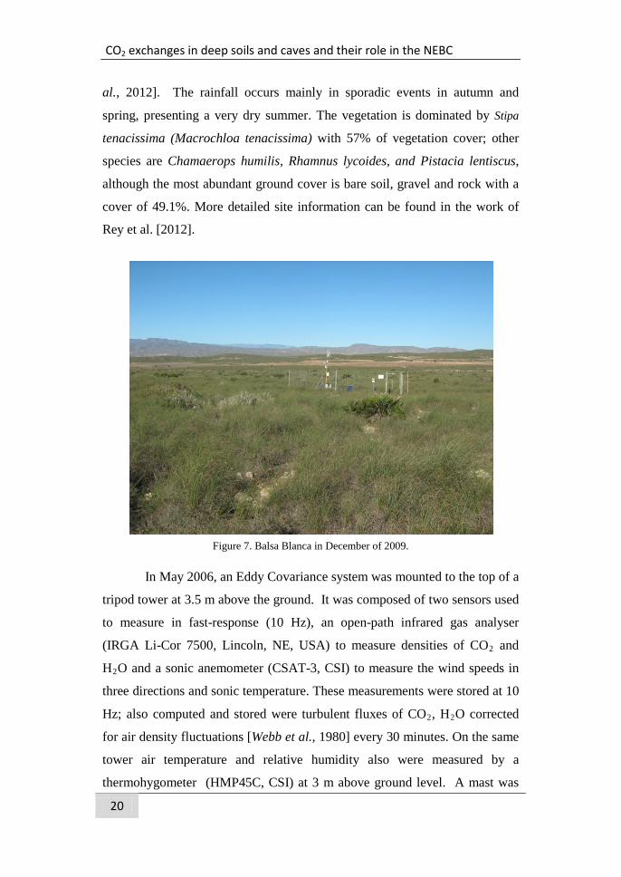
3.2 Balsa Blanca
Balsa Blanca is located in the Cabo de Gata-Nijar Natural Park of
southeast Spain (N36º56’26.0’’, W2º0.1’58.8’’). This is an alpha grass steppe
at 200 m a.s.l situated on alluvial fans (glacis) of gentle slope (2%). The soil is
classified as Calcaric Lithic Leptosol saturated in carbonates with 10cm depth
on average, presenting petrocalcic horizons. The mean annual temperature is
around 18ºC with maximum in summer (37ºC) and minimum in winter (1ºC).
The climate is dry subtropical semiarid, with a mean annual precipitation of
ca. 200 mm and an annual potential evapotranspiration around 1390 mm with
an aridity index below 0.2, classifying this area as an arid zone [Oyonarte et
CO2 exchanges in deep soils and caves and their role in the NEBC
20
al., 2012]. The rainfall occurs mainly in sporadic events in autumn and
spring, presenting a very dry summer. The vegetation is dominated by Stipa
tenacissima (Macrochloa tenacissima) with 57% of vegetation cover; other
species are Chamaerops humilis, Rhamnus lycoides, and Pistacia lentiscus,
although the most abundant ground cover is bare soil, gravel and rock with a
cover of 49.1%. More detailed site information can be found in the work of
Rey et al. [2012].
Figure 7. Balsa Blanca in December of 2009.
In May 2006, an Eddy Covariance system was mounted to the top of a
tripod tower at 3.5 m above the ground. It was composed of two sensors used
to measure in fast-response (10 Hz), an open-path infrared gas analyser
(IRGA Li-Cor 7500, Lincoln, NE, USA) to measure densities of CO2 and
H2O and a sonic anemometer (CSAT-3, CSI) to measure the wind speeds in
three directions and sonic temperature. These measurements were stored at 10
Hz; also computed and stored were turbulent fluxes of CO2, H2O corrected
for air density fluctuations [Webb et al., 1980] every 30 minutes. On the same
tower air temperature and relative humidity also were measured by a
thermohygometer (HMP45C, CSI) at 3 m above ground level. A mast was
Experimental Field Sites
21
installed at 8 m from the eddy tower to measure at 1.5 m above ground level
incident and reflected photosynthetically active radiation (PAR, LI-190, Li-
Cor ), a net radiometer (NR-Lite, Kipp&Zonnen, Netherlands) and an tipping-
bucket rain gauge (ARG100, CSI). Below ground, the soil heat flux was
measured by four soil heat flux plates at 8 cm (HFP01SC, CSI), soil
temperature was measured by two averaging soil thermocouple probes
(TCAV, CSI) and soil moisture by two water content reflectometers (CS616,
CSI). All data were measured at 10 Hz, averaged over 30 minutes, and
recorded by a data-logger (CR3000, CSI).
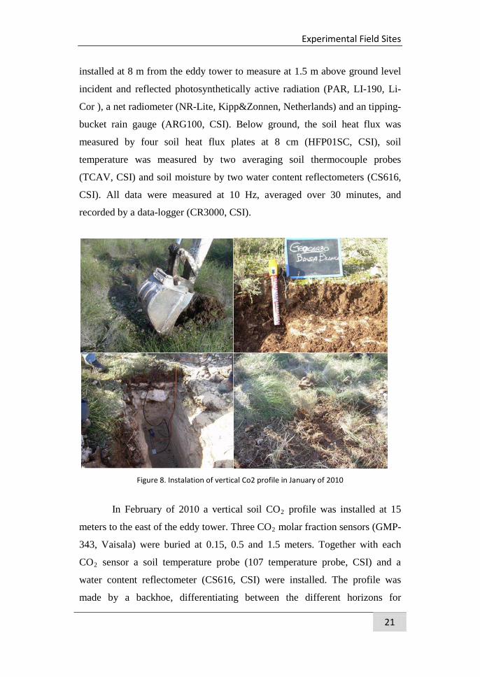
Figure 8. Instalation of vertical Co2 profile in January of 2010
In February of 2010 a vertical soil CO2 profile was installed at 15
meters to the east of the eddy tower. Three CO2 molar fraction sensors (GMP-
343, Vaisala) were buried at 0.15, 0.5 and 1.5 meters. Together with each
CO2 sensor a soil temperature probe (107 temperature probe, CSI) and a
water content reflectometer (CS616, CSI) were installed. The profile was
made by a backhoe, differentiating between the different horizons for

CO2 exchanges in deep soils and caves and their role in the NEBC
22
subsequent burial of the sensors, each in its own soil horizon. Measurements
were made every 30s and stored as 5 minutes averages by a data-logger.
Experimental Field Sites
23
References
Amiro, B. D., J. Ian MacPherson, R. L. Desjardins, J. M. Chen, and J. Liu
(2003), Post-fire carbon dioxide fluxes in the western Canadian boreal
forest: evidence from towers, aircraft and remote sensing., Agric. For.
Meteorol., 115, 91 - 107.
Anthoni, P. M., A. knohl, C. Rebmann, A. Freibauer, M. Mund, W. Ziegler,
O. Kolle, and E.-D. Schulze (2004), Forest and agricultural land-use-
dependent CO2 exchange in Thurigia, Germany, Glob. Change Biol.,
10, 2005-2019.
Aubinet, M., C. Moureaux, B. Bodson, D. Dufranne, B. Heinesch, M. Suleau,
F. Vancutsem, and A. Vilret (2009), Carbon sequestration by a crop
over a 4-year sugar beet/winter wheat/seed potato/winter wheat
rotation cycle, Agric. For. Meteorol., 149(3-4), 407-418.
Aubinet, M., T. Vesala, and D. Papale (2012), Eddy Covariance: A Practical
Guide to Measurement and Data Analysis, 438 pp., Springer.
Baldocchi, D. D. (2003), Assessing the eddy covariance technique for
evaluating carbon dioxide exchange rate of ecosystem: past, present
and future, Glob. Change Biol., 9, 479-492.
Baldocchi, D., et al. (2001), FLUXNET: A new tool to study the temporal and
spatial variability of ecosystem-scale carbon dioxide, water vapor, and
energy flux densities, Bull. Amer. Meteorol. Soc., 82(11), 2415-2434.
Boix-Fayos, C., J. de Vente, J. Albaladejo, and M. Martinez-Mena (2009),
Soil carbon erosion and stock as affected by land use changes at the
catchment scale in Mediterranean ecosystems, Agriculture
Ecosystems & Environment, 133(1-2), 75-85.
Boucot, A. J., and J. Gray (2001), A critique of Phanerozoic climatic models
involving changes in the CO2 content of the atmosphere, Earth-
Science Reviews, 56(1–4), 1-159.
CO2 exchanges in deep soils and caves and their role in the NEBC
24
Brandt, L. A., C. Bohnet, and J. Y. King (2009), Photochemically induced
carbon dioxide production as a mechanism for carbon loss from plant
litter in arid ecosystems, J. Geophys. Res.-Biogeosci., 114.
Burba, G. G., D. K. McDermitt, A. Grelle, D. J. Anderson, and L. Xu (2008),
Addressing the influence of instrument surface heat exchange on the
measurements of CO(2) flux from open-path gas analyzers, Glob.
Change Biol., 14(8), 1854-1876.
Canadell, J. G., C. Le Quere, M. R. Raupach, C. B. Field, E. T. Buitenhuis, P.
Ciais, T. J. Conway, N. P. Gillett, R. A. Houghton, and G. Marland
(2007), Contributions to accelerating atmospheric CO(2) growth from
economic activity, carbon intensity, and efficiency of natural sinks,
Proceedings of the National Academy of Sciences of the United States
of America, 104(47), 18866-18870.
Carrara, A., I. A. Janssens, J. C. Yuste, and R. Ceulemans (2004), Seasonal
changes in photosynthesis, respiration and NEE of a mixed temperate
forest, Agric. For. Meteorol., 126, 15-31.
Chapin, F. S., et al. (2006), Reconciling carbon-cycle concepts, terminology,
and methods, Ecosystems, 9(7), 1041-1050.
Crowther, J. (1983), Carbon dioxide concentrations in some tropical karst
soils, west Malaysia, Catena, 10(1-2), 27-39.
Denis, A., R. Lastennet, F. Huneau, and P. Malaurent (2005), Identification of
functional relationships between atmospheric pressure and CO2 in the
cave of Lascaux using the concept of entropy of curves, Geophys.
Res. Lett., 32(5).
Ek, C., and M. Gewelt (1985), Carbon dioxide in cave atmospheres. New
results in Belgium and comparison with some other countries., Earth
Surf. Process. Landf., 10(2), 173-187.
Emmerich, E. W. (2003), Carbon dioxide fluxes in a semiarid environment
with high carbonate soils, Agric. For. Meteorol., 116, 91-102.
Eswaran, H., E. V. D. Berg, and P. Reich (1993), Organic Carbon in Soils of
the World, Soil Science Society of America, 57.
Experimental Field Sites
25
Falge, E., et al. (2002), Seasonality of ecosystem respiration and gross
primary production as derived from FLUXNET measurements, Agric.
For. Meteorol., 113(1-4), 53-74.
Ford, D. C., and P. W. Williams (1989), Karst Geomorphology and
Hydrology, 601 pp., London.
Hasting, S. J., W. C. Oechel, and A. Muhlia-Melo (2005), Diurnal, seasonal
and annual variation in the net ecosystem CO2 exchange of a desert
shrub community (Sarcocaulescent) in Baja California, Mexico, Glob.
Change Biol., 11, 1-13.
Houghton, R. A. (2002), Terrestrial carbon sink, Biologist, 49(4), 155-160.
Howarth, F. G., and F. D. Stone (1990), Elevated carbon dioxide levels in
Bayliss Cave, Australia: implications for the evolution of obligate
cave species., Pacific Science, 44(3), 207-218.
IPCC 2007, Solomon, S., D. Qin, M. Manning, Z. Chen, M. Marquis, K. B.
Averyt, M. Tignor, and H. L. Miller (2007), Contribution of Working
Group I to the Fourth Assessment Report of the Intergovernmental
Panel on Climate Change, 2007 996 pp., Cambridge University Press,
Cambridge.
Jacinthe, P. A., and R. Lal (2001), A mass balance approach to assess carbon
dioxide evolution during erosional events, Land Degradation &
Development, 12(4), 329-339.
Keeling, C. D. (1960), The concentration and isotopic abundance of carbon
dioxide in the atmosphere., Tellus, 12, 200-203.
Kirschbaum, M. U. F. (2000), Will changes in soil organic carbon act as a
positive or negative feedback on global warning?, Biogeochemistry,
48, 21-51.
Kowalski, A. S., M. Sartore, R. Burlett, P. Berbigier, and D. Loustau (2003),
The annual carbon budget of a French pine forest (Pinus pinaster)
following harvest, Glob. Change Biol., 9(7), 1051-1065.
Kowalski, A. S., P. Serrano-Ortiz, I. A. Janssens, S. Sanchez-Moraic, S.
Cuezva, F. Domingo, A. Were, and L. Alados-Arboledas (2008), Can
CO2 exchanges in deep soils and caves and their role in the NEBC
26
flux tower research neglect geochemical CO2 exchange?, Agric. For.
Meteorol., 148(6-7), 1045-1054.
Kowalski, A. S., et al. (2004), Paired comparisons of carbon exchange
between undisturbed and regenerating stands in four managed forests
in Europe, Glob. Change Biol., 10(10), 1707-1723.
McDermitt, D. K., J. M. Welles, and R. D. Eckles (1994), Effects of
temperature, pressure and water vapor on gas phase infrared
absorption by CO2, App. Note #116. Li-Cor Inc., Lincoln, NE.
Mielnick, P., W. A. Dugas, K. Mitchell, and K. Havstad (2005), Long-term
measurements of CO2 flux and evapotranspiration in a Chihuahuan
desert grassland, J. Arid. Environ., 60(3), 423-436.
Oyonarte, C., A. Rey, J. Raimundo, I. Miralles, and P. Escribano (2012), The
use of soil respiration as an ecological indicator in arid ecosystems of
the SE of Spain: Spatial variability and controlling factors, Ecol.
Indic., 14(1), 40-49.
Plummer L, N., L. Parkhurst D, and L. Wigley T. M (1979), Critical Review
of the Kinetics of Calcite Dissolution and Precipitation, in Chemical
Modeling in Aqueous Systems, edited, pp. 537-573, American
Chemical Society.
Reichstein, M., et al. (2005), On the separation of net ecosystem exchange
into assimilation and ecosystem respiration: review and improved
algorithm, Glob. Change Biol., 11(9), 1424-1439.
Reverter, B. R. (2011), Intercambios de CO2 y vapor de agua en ecosistemas
de alta montaña de matorral mediterráneo, 279 pp, Universidad de
Granada, Granada.
Reverter, B. R., E. P. Sanchez-Canete, V. Resco, P. Serrano-Ortiz, C.
Oyonarte, and A. S. Kowalski (2010), Analyzing the major drivers of
NEE in a Mediterranean alpine shrubland, Biogeosciences, 7(9),
2601-2611.
Experimental Field Sites
27
Reverter, B. R., et al. (2011), Adjustment of annual NEE and ET for the open-
path IRGA self-heating correction: Magnitude and approximation
over a range of climate, Agric. For. Meteorol., 151(12), 1856-1861.
Rey, A., L. Belelli-Marchesini, A. Were, P. Serrano-Ortiz, G. Etiope, D.
Papale, F. Domingo, and E. Pegoraro (2012), Wind as a main driver
of the net ecosystem carbon balance of a semiarid Mediterranean
steppe in the South East of Spain, Glob. Change Biol., 18(2), 539-
554.
Schlesinger, W. H. (1997), Biogeochemistry: An Analysis of Global Change,
2 ed., 588 pp., Academic Press, San Diego.
Scott, R. L., P. Serrano-Ortiz, F. Doming, E. P. Hamerlynck, and A. S.
Kowalski (2012), Commonalities of carbon dioxide exchange in
semiarid regions with monsoon and Mediterranean climates, J. Arid.
Environ., 84, 71-79.
Serrano-Ortiz, P. (2008), Intercambios de CO2 entre atmósfera y ecosistemas
kársticos: aplicabilidad de las técnicas comúnmente empleadas., 305
pp, Universidad de Granada, Granada.
Serrano-Ortiz, P., E. Sánchez-Cañete, and C. Oyonarte (2012), The Carbon
Cycle in Drylands, in Recarbonization of the Biosphere, edited by R.
Lal, K. Lorenz, R. F. Hüttl, B. U. Schneider and J. von Braun, pp.
347-368, Springer Netherlands.
Serrano-Ortiz, P., S. Maranon-Jimenez, B. R. Reverter, E. P. Sanchez-Canete,
J. Castro, R. Zamora, and A. S. Kowalski (2011), Post-fire salvage
logging reduces carbon sequestration in Mediterranean coniferous
forest, Forest Ecology and Management, 262(12), 2287-2296.
Serrano-Ortiz, P., F. Domingo, A. Cazorla, A. Were, S. Cuezva, L.
Villagarcia, L. Alados-Arboledas, and A. S. Kowalski (2009),
Interannual CO2 exchange of a sparse Mediterranean shrubland on a
carbonaceous substrate, J. Geophys. Res.-Biogeosci., 114, G04015.
Stull, R. B. (1988), An introduction to Boundary Layer Meteorology, 667 pp.,
Kluwer Academic Publishers, Dordrecht, The Netherlands.
CO2 exchanges in deep soils and caves and their role in the NEBC
28
Valentini, R., et al. (2000), Respiration as the main determinant of carbon
balance in European forests, Nature, 404, 861 - 865.
Vallejos, A., A. Pulido-Bosch, and W. Martin-Rosales (1997), Contribution of
environmental isotopes to the understanding of complex hydrologic
systems. A case study: Sierra de Gador, SE Spain, Earth Surf.
Process. Landf., 22(12), 1157-1168.
Verrecchia, E. P., J. L. Dumont, and K. E. Rolko (1990), Do fungi building
limestones exist in semiarid regions?, Naturwissenschaften, 77(12),
584-586.
Webb, E. K., G. I. Pearman, and R. Leuning (1980), Correction of flux
measurements for density effects due to heat and water vapor transfer,
Q. J. R. Meteorol. Soc., 106(447), 85-100.
Were, A., P. Serrano-Ortiz, C. M. de Jong, L. Villagarcia, F. Domingo, and A.
S. Kowalski (2010), Ventilation of subterranean CO2 and Eddy
covariance incongruities over carbonate ecosystems, Biogeosciences,
7(3), 859-867.
Wohlfahrt, G., L. F. Fenstermaker, and J. A. Arnone (2008), Large annual net
ecosystem CO2 uptake of a Mojave Desert ecosystem, Glob. Change
Biol., 14, 1475-1487.

Experimental Field Sites
29

CO2 exchanges in deep soils and caves and their role in the NEBC
30

Results
31
4. Results

CO2 exchanges in deep soils and caves and their role in the NEBC
32
Results. Chapter 1
33
4.1 Chapter 1
A New Definition of the Virtual Temperature, Valid for the Atmosphere and the CO2-Rich Air of the
Vadose Zone
Kowalski A.S. 1,2 & Sanchez-Cañete, E.P.2,3.
Published in Journal of Applied Meteorology and Climatology.
Kowalski, A. S., and E. P. Sanchez-Canete (2010), A New Definition of the Virtual Temperature, Valid for the Atmosphere and the CO2-Rich Air of the Vadose Zone, Journal of Applied Meteorology and Climatology, 49(8), 1692-1695.
A New Definition of the Tv, Valid for the Atmosphere and the CO2-Rich Air.
34
Abstract
In speleological environments, partial pressures of carbon dioxide
(CO2) are often large enough to affect overall air density. Excluding this gas
when defining the gas constant for air, a new definition is proposed for the
virtual temperature Tv that remains valid for the atmosphere in general but
furthermore serves to examine the buoyancy of CO2-rich air in caves and
other subterranean airspaces.
Results. Chapter 1
35
4.1.1. Introduction
In recent years, boundary layer meteorology has broadened to explore
surface–atmosphere interactions involving exchanges with caves and other
airspaces of the vadose zone. The accumulation and subsequent ventilation of
large [Kowalski et al., 2008; Milanolo and Gabrovsek, 2009] quantities of
carbon dioxide (CO2) in such environments implies a potentially significant
yet previously overlooked role for them in the global carbon cycle [Serrano-
Ortiz et al., 2009], whose characterization remains a Kyoto-motivated
challenge. Gas exchange in the vadose zone can come about via convection
[Weisbrod et al., 2009], which is sometimes invoked to suggest a dependence
of cave ventilation on the temperature difference with the external atmosphere
[Fernandez-Cortes et al., 2009; Kowalczk and Froelich, 2010; Linan et al.,
2008].
However, differences in air density at a given pressure level (altitude)
are determined not only by temperature but also by air composition. In the
troposphere, the only gas whose surface exchange and fluctuating partial
pressure appreciably affect air density is water vapor, which varies from near
0% (volumetric) in cold environments to 4% in the tropics, and locally in the
presence of evaporation. Thus, meteorologists employ a traditional definition
of the virtual temperature (Tv) to account for air density variations associated
with the molecular weight of water vapor [Guldberg and Hohn 1876; Wallace
and Hobbs 2006]. By contrast, in speleological environments volumetric
fractions of CO2 have been often observed to exceed a few percent [Ek and
Gewelt, 1985], a fact which highlights the need for an expanded definition of
Tv for the purpose of studying air buoyancy in such spaces.
We propose a redefinition of Tv to accommodate such CO2-rich air
without compromising its validity for use in the atmosphere in general,
including comparison with the traditional definition of Tv.
A New Definition of the Tv, Valid for the Atmosphere and the CO2-Rich Air.
36
4.1.2. Analyses and approximations
In the following development, subscripts are used to identify
individual gases including water vapor (v) and CO2 (c), as well as gas
mixtures defined by the mixture of nitrogen, oxygen, and argon (noa), ‘‘dry
air’’ (d), and the overall mixture of moist air including CO2 (mc).
The fundamental change proposed here is to substitute the mixture of
nitrogen, oxygen, and argon for the traditional dry air, both in defining the
nonvariable gas constant and also in the denominators defining the mixing
ratios for water vapor (rv) and carbon dioxide (rc). Such a substitution
modifies tropospheric values of rv and rc by less than 0.06% relative to the
traditional definitions, according to the current mass fraction of CO2 in such
air.
The gas constant for the mixture mc shows variable behavior
according to the mass M contributed by each constituent, weighting that
constituent’s gas constant:
cvnoa
ccvvnoanoamc MMM
RMRMRMR++
++= (eq. 1)
This is the constant that must be used when expressing the gas law
TRp mcρ= for the moist, CO2-laden air of a subterranean airspace. Dividing
both numerator and denominator of Eq. (1) by Mnoa leaves
cv
ccvvnoamc rr
RrRrRR++
++=
1 (eq. 2)
Generally this can be expressed
Results. Chapter 1
37
( )
+
+=
∑∑
=
=Ni i
Ni ii
noamcr
rRR
1
1
1
1 ε (eq. 3)
which can be expanded to consider other gases for other applications.
Equation (2) can be manipulated by multiplying both numerator and
denominator by the factor (1 – rv - rc) to yield an expression that is complex
but suitable for approximation:
22
22
21 ccvv
ccccvccvcvvvvvnoacnoavnoamc rrrr
RrRrrRrRrrRrRrRrRrRR−−+
−−+−−+−−= (eq. 4)
The denominator of Eq. (4) can be approximated as unity when
recognizing that every second-order term is several orders of magnitude
smaller. Similarly, second-order terms may be safely neglected in the
numerator, simplifying to the following approximation:
ccvvnoacnoavnoamc RrRrRrRrRR ++−−= (eq. 5)
Substituting the gas constants for the noa mixture (287.0 J K-1 kg-1;
practically identical to that of dry air), water vapor (461.5 J K-1 kg-1), and CO2
(188.9 J K-1 kg-1) into Eq. (5) allows an approximate definition of the
(variable) gas constant for the moist, CO2-laden mixture as
( )cvnoamc rrRR 3419.06079.01 −+= (eq. 6)
Finally, in the context of the gas law, shifting the variability caused by
constituent fluctuations from the gas constant to the virtual temperature results
in the following new definition:
( )cvv rrTT 3419.06079.01 −+= (eq. 7)
A New Definition of the Tv, Valid for the Atmosphere and the CO2-Rich Air.
38
This is the temperature that a mixture of nitrogen, oxygen, and argon
would need in order to equal the density of the mixture of moist air including
CO2; it allows us to compare the densities of any (cave or atmospheric) air at
equal pressures. Furthermore, this version of Tv can be used to compute the
density of cave air from pressure using the gas law vnoaTRp ρ= (with Rnoa =
287.0 J K-1 kg-1) and compared with the traditional Tv for atmospheric air.
4.1.3. Implications and validity
The ramifications of the proposed change in definition depend
directly on the CO2 mixing ratio. In the troposphere, this is currently around
0.587 g kg-1, equivalent to 387 ppm, or 0.0387% volumetric (fractional CO2
content is expressed hereinafter in volumetric terms to correspond to the data
typically reported in both speleological and atmospheric literature). For such
low atmospheric CO2 fractions the difference between the traditional
definition of Tv and that defined in Eq. (7) is generally less than 0.1ºC.
However, high levels of CO2 in cave atmospheres can lead to situations where
using the inappropriate definition of Tv (or simply the temperature) can lead
to erroneous conclusions regarding buoyancy and the onset of convective
processes.
A preliminary climatology of vadose-zone CO2 volumetric fractions
[Ek and Gewelt, 1985] indicated that while caves in subpolar and cold-
temperate boreal zones rarely exceed double the atmospheric concentration
(well below 0.1%), much larger values can be found in cool–temperate zones
inside caves (approaching 1%), and particularly in fissures, sometimes
exceeding 6% [Denis et al., 2005]. More modest values have been reported in
continental and subcontinental caves, but indications from warmer climates
suggest that CO2 volumetric fractions in excess of 5% can be reached,
particularly in poorly ventilated fissures [Benavente et al., 2010]. For such
extreme cases the virtual temperature can differ from the air temperature by
Results. Chapter 1
39
many degrees, and the former must be used to draw accurate conclusions
about comparative density.
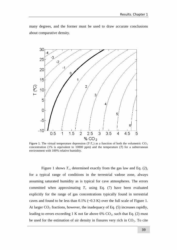
Figure 1. The virtual temperature depression (T-Tv) as a function of both the volumetric CO2 concentration (1% is equivalent to 10000 ppm) and the temperature (T) for a subterranean environment with 100% relative humidity.
Figure 1 shows Tv, determined exactly from the gas law and Eq. (2),
for a typical range of conditions in the terrestrial vadose zone, always
assuming saturated humidity as is typical for cave atmospheres. The errors
committed when approximating Tv using Eq. (7) have been evaluated
explicitly for the range of gas concentrations typically found in terrestrial
caves and found to be less than 0.1% (~0.3 K) over the full scale of Figure 1.
At larger CO2 fractions, however, the inadequacy of Eq. (5) increases rapidly,
leading to errors exceeding 1 K not far above 6% CO2, such that Eq. (2) must
be used for the estimation of air density in fissures very rich in CO2. To cite
A New Definition of the Tv, Valid for the Atmosphere and the CO2-Rich Air.
40
one example, for the Shaft of the Dead Man in the French Lascaux cave in
late January 2001 with 6% CO2 [Denis et al., 2005], Tv is 6.9ºC lower than
the cave air temperature (14ºC), explaining the stagnancy of this airspace
exceeding the CO2 limits for human safety [Hoyos et al., 1998].
We propose defining Tv as in Eq. (7) for caves and other situations
with volumetric CO2 fractions ranging from a few tenths of a percent, up to
5%.
Acknowledgements
This work was supported by the Andalusian regional government
project GEOCARBO (P08-RNM-3721), by the Spanish National Institute for
Agronomic Research (INIA, SUM2006-00010), and also by the European
Commission project GHG Europe (FP7-ENV-2009-1).
Results. Chapter 1
41
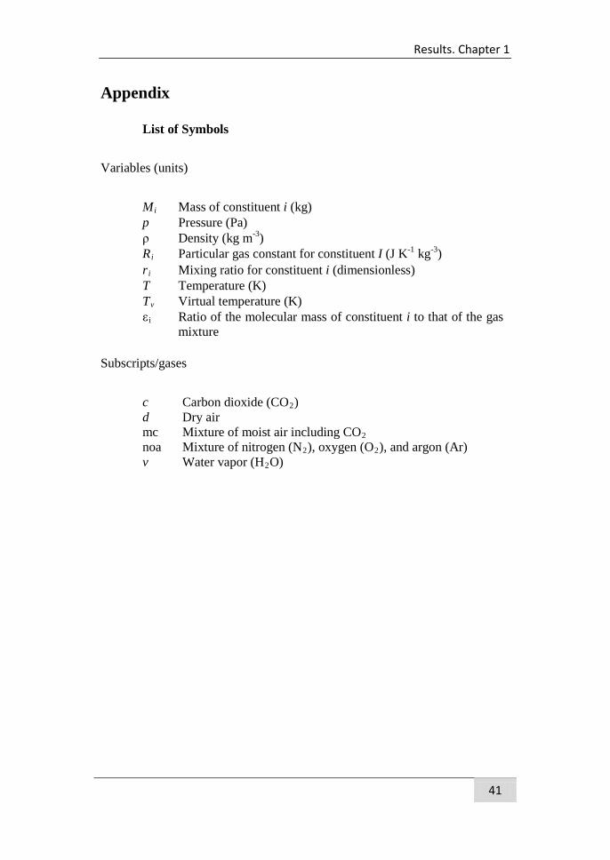
Appendix
List of Symbols
Variables (units)
Mi Mass of constituent i (kg) p Pressure (Pa) ρ Density (kg m-3) Ri Particular gas constant for constituent I (J K-1 kg-3) ri Mixing ratio for constituent i (dimensionless) T Temperature (K) Tv Virtual temperature (K) ε i Ratio of the molecular mass of constituent i to that of the gas
mixture
Subscripts/gases
c Carbon dioxide (CO2) d Dry air mc Mixture of moist air including CO2 noa Mixture of nitrogen (N2), oxygen (O2), and argon (Ar) v Water vapor (H2O)
A New Definition of the Tv, Valid for the Atmosphere and the CO2-Rich Air.
42
References
Benavente, J., I. Vadillo, F. Carrasco, A. Soler, C. Linan, and F. Moral
(2010), Air Carbon Dioxide Contents in the Vadose Zone of a
Mediterranean Karst, Vadose Zone J., 9(1), 126-136.
Denis, A., R. Lastennet, F. Huneau, and P. Malaurent (2005), Identification of
functional relationships between atmospheric pressure and CO2 in the
cave of Lascaux using the concept of entropy of curves, Geophys.
Res. Lett., 32(5).
Ek, C., and M. Gewelt (1985), Carbon dioxide in cave atmospheres. New
results in Belgium and comparison with some other countries., Earth
Surf. Process. Landf., 10(2), 173-187.
Fernandez-Cortes, A., S. Sanchez-Moral, S. Cuezva, D. Benavente, and R.
Abella (2009), Characterization of trace gases' fluctuations on a 'low
energy' cave (Castanar de Ibor, Spain) using techniques of entropy of
curves, Int. J. Climatol., 31(1), 127-143.
Guldberg, C. M., and H. Hohn, 1876:E ´ tudes sur les Mouvements de
l’Atmosphe` re (Studies on the Movement of the Atmosphere). Part 1.
Christiania Academy of Sciences, 39 pp.
Hoyos, M., V. Soler, J. C. Cañaveras, S. Sánchez-Moral, and E. Sanz-Rubio
(1998), Microclimatic characterization of a karstic cave: human
impact on microenvironmental parameters of a prehistoric rock art
cave (Candamo Cave, northern Spain), Environ. Geol., 33(4), 231-
242.
Kowalczk, A. J., and P. N. Froelich (2010), Cave air ventilation and CO2
outgassing by radon-222 modeling: How fast do caves breathe?, Earth
Planet. Sci. Lett., 289(1-2), 209-219.
Kowalski, A. S., P. Serrano-Ortiz, I. A. Janssens, S. Sanchez-Moraic, S.
Cuezva, F. Domingo, A. Were, and L. Alados-Arboledas (2008), Can
flux tower research neglect geochemical CO2 exchange?, Agric. For.
Meteorol., 148(6-7), 1045-1054.
Results. Chapter 1
43
Linan, C., I. Vadillo, and F. Carrasco (2008), Carbon dioxide concentration in
air within the Nerja Cave (Malaga, Andalusia, Spain), Int. J. Speleol.,
37(2), 99-106.
Milanolo, S., and F. Gabrovsek (2009), Analysis of Carbon Dioxide
Variations in the Atmosphere of Srednja Bijambarska Cave, Bosnia
and Herzegovina, Bound.-Layer Meteor., 131(3), 479-493.
Serrano-Ortiz, P., F. Domingo, A. Cazorla, A. Were, S. Cuezva, L.
Villagarcia, L. Alados-Arboledas, and A. S. Kowalski (2009),
Interannual CO2 exchange of a sparse Mediterranean shrubland on a
carbonaceous substrate, J. Geophys. Res.-Biogeosci., 114, G04015.
Wallace, J. M., and P. V. Hobbs, 2006: Atmospheric Science: An Introductory
Survey. Academic Press, 483 pp.
Weisbrod, N., M. I. Dragila, U. Nachshon, and M. Pillersdorf (2009), Falling
through the cracks: The role of fractures in Earth-atmosphere gas
exchange, Geophys. Res. Lett., 36.

A New Definition of the Tv, Valid for the Atmosphere and the CO2-Rich Air.
44
Results. Chapter 2
45
4.2 Chapter 2
Cave ventilation is influenced by variations in the CO2-dependent virtual temperature
Sanchez-Cañete, E.P.1,2 Serrano-Ortiz, P.1,2 Domingo, F. 1,3 Kowalski, A.S.2,4.
Published in International Journal of Speleology
Sanchez-Canete, E. P., P. Serrano-Ortiz, F. Domingo, and A. S. Kowalski (2013), Cave ventilation is influenced by variations in the CO2-dependent virtual temperature, International Journal of Speleology, 42 (1), 1-8.
Cave ventilation is influenced by variations in the CO2-dependent Tv.
46
Abstract
Dynamics and drivers of ventilation in caves are of growing interest
for different fields of science. Accumulated CO2 in caves can be exchanged
with the atmosphere, modifying the internal CO2 content, affecting stalagmite
growth rates, deteriorating rupestrian paintings, or creating new minerals.
Current estimates of cave ventilation neglect the role of high CO2
concentrations in determining air density – approximated via the virtual
temperature (Tv) –, affecting buoyancy and therefore the release or storage of
CO2. Here we try to improve knowledge and understanding of cave ventilation
through the use of Tv in CO2-rich air to explain buoyancy for different values
of temperature (T) and CO2 content. Also, we show differences between T
and Tv for 14 different experimental sites in the vadose zone, demonstrating
the importance of using the correct definition of Tv to determine air buoyancy
in caves. The calculation of Tv (including CO2 effects) is currently available
via internet using an excel template, requiring the input of CO2 (%), air
temperature (ºC) and relative humidity (%).
Results. Chapter 2
47
4.2.1. Introduction
There is currently growing interest in characterizing storage and
ventilation of CO2 in caves, both from external (atmospheric) and internal
(speleological) perspectives. Measurements of rising atmospheric CO2 by
Keeling [1960] since the mid-20th century reveal that anthropogenic activities
are causing CO2 accumulation in the atmosphere and forcing global warming.
Soils are a large pool of terrestrial carbon (C), estimated to contain 2344 Pg C
in solid form in the top 3 m [Jobbagy and Jackson, 2000] – three times the
aboveground biomass C reservoir and double that of the atmosphere
[Schlesinger, 1997] – and also have an enormous capacity to store gaseous
CO2 in subsurface cracks, pores and cavities. The vadose zone is enriched in
CO2 and some caves often exceed 5% [volumetric CO2 fraction of 50,000
ppm; [Batiot-Guilhe et al., 2007; Benavente et al., 2010; Denis et al., 2005;
Ek and Gewelt, 1985; Howarth and Stone, 1990] representing important air
compositional differences with respect to the external atmosphere, currently
near 395 ppm. Accumulated CO2 in caves can be exchanged with the
atmosphere [Sanchez-Canete et al., 2011; Serrano-Ortiz et al., 2010;
Weisbrod et al., 2009], modifying the internal CO2 content and affecting
stalagmite growth rates [Baldini et al., 2008; Banner et al., 2007],
deteriorating rupestrian paintings [Fernández et al., 1986] and creating new
minerals [Badino et al., 2011]. However due to the complexity and peculiarity
of caves, as well as the variety of meteorological conditions that determine the
degree and timing of ventilation [Fairchild and Baker, 2012], such exchanges
are not well understood and their contributions to regional atmospheric CO2
budgets remain unknown.
Estimation of cave ventilation can be realized by a number of means,
the most common of which has traditionally neglected the role of high CO2
concentrations and requires refinement. The drivers implicated in the cave
ventilation can be classified as either dynamic or static [Cigna, 1968].
Cave ventilation is influenced by variations in the CO2-dependent Tv.
48
Dynamic drivers are defined by moving fluids such as water or wind
[Nachshon et al., 2012], while static drivers include variations of pressure,
temperature or air composition (water vapor, CO2, CH4, etc.). Ventilation
rates can be measured directly using anemometers, estimated indirectly
through variations in Radon content [Faimon et al., 2006; Hakl et al., 1997],
or other tracer gases [de Freitas et al., 1982] or variations in air density. Most
commonly, air density variations are approximated to evaluate buoyancy
according to temperature differences between the internal (Tint) and exterior
atmosphere (Text), neglecting air composition [Baldini et al., 2008; Faimon et
al., 2012; Fernandez-Cortes et al., 2006; Linan et al., 2008; Milanolo and
Gabrovsek, 2009]. Faimon et al. [2012] modelled the airflows into a cave, and
found that the temperature explained more than 99% of variations in air
density; therefore, temperature could be used as an alternative airflow
predictor. However, de Freitas et al. [1982] concluded that reversal of airflow
occurs when the densities in the cave and the exterior are equal, rather than
when thermal conditions of the cave and external air are the same. For this
reason, they suggest that the gradient in virtual temperature (Tv) between the
cave and outside air would be the appropriate indicator. In this sense,
Kowalczk & Froelich [2010], improved the determination of internal /external
air densities by including the influence of water vapor, using the traditional
definition of the virtual temperature. Nevertheless, in cases where CO2 molar
fractions of internal air exceed atmospheric values by an order of magnitude
or more, it is necessary to take into account the heaviness of CO2 when
calculating the virtual temperature [Kowalski and Sanchez-Canete, 2010].
Whereas high CO2 values registered in cave air have been attributed
most often to the seepage of CO2-enriched water from the root zone, the
possibility of sinking flows of dense, CO2-rich air should also be considered.
Biological CO2 is produced near the surface by respiration of plant roots and
microorganisms [Kuzyakov, 2006]; in most caves, isotopic studies confirm a
clear biological origin of cave CO2 [Bourges et al., 2001; Bourges et al.,
Results. Chapter 2
49
2012]. Soil CO2 generally increases with depth, from near-atmospheric
concentrations at a few centimeters to an order of magnitude more a few
meters down [Amundson and Davidson, 1990; Atkinson, 1977]. High
concentrations of CO2 at depth have been explained in terms of shallow CO2
dissolution, downward transport by seepage, and subsequent precipitation
from water in deeper layers [Spotl et al., 2005], whereas surface layers are
depleted in CO2 by exchange with the atmosphere. At depth and for caves in
particular, another input of CO2 could be due to the injection of dense, CO2-
rich air, flowing down through fissures due to differences in buoyancy, whose
characterization is poorly known and requires information regarding Tv. This
virtual temperature has been little applied to soils and caves, but could explain
why CO2 accumulates at depth yielding concentrations much higher than
those in the atmosphere.
Here we show the error produced in determining the virtual
temperature when not taking into account CO2 effects, and demonstrate its
repercussions for the determination of air buoyancy in caves. We try to
improve knowledge and understanding of cave ventilation through the use of
virtual temperature in CO2-rich air. Accurate determinations of virtual
temperature allow numerical evaluation of buoyancy, and thus can determine
exactly when ventilation is possible, and therefore when a cave can release or
store CO2. Also we represent Tv - explaining the relative buoyancy relevant
for cave ventilation - for different values of T and CO2 content. Then, we
show differences between T and Tv, - calculated both with and without
accounting for CO2 content - for 14 different experimental sites in the vadose
zone, demonstrating the importance of using the correct definition of Tv to
determine air buoyancy in caves.
Cave ventilation is influenced by variations in the CO2-dependent Tv.
50
4.2.2. Derivations and definitions
For purposes of characterizing air buoyancy, meteorologists define
the virtual temperature (Tv) as the temperature that dry air must have to equal
the density of moist air at the same pressure. The virtual temperature for the
atmosphere is approximated as (see appendix A):
( )rTTv 61.01+= (eq. 1)
where T and Tv are the absolute temperature (K) and virtual
temperature (K) respectively and r is the mixing ratio (dimensionless),
defined as the ratio of the mass of water vapor to that of dry air.
Thus variations in the virtual temperature serve as a proxy for those in
air density (Stull, 1988), which can be obtained through the equation of state
for moist air:
vdTRp ρ= (eq. 2)
where p, ρ and Rd are the pressure (Pa=J m-3), air density (kg m-3) and
particular gas constant for dry air (286.97 J kg-1 K-1) respectively. Equation
(2) makes clear that, for a given altitude level (pressure), air density is related
directly to Tv, which serves therefore as a surrogate variable for determining
buoyancy.
Equation (2) is only valid for the free atmosphere, while for caves or
soils it should not be used due to high concentrations of CO2 in the air. This
equation, normally used for assessing the buoyancy of an air mass by changes
in its density, is valid in the atmosphere because the molar mass of dry air
(md) is very constant, 0.02897 kg·mol-1, since air composition is very constant
once water vapor has been excluded. However the air composition in soils or
caves differs from that of the atmosphere due to higher amounts of CO2.
Results. Chapter 2
51
The correct equations to calculate the virtual temperature including
CO2 effects were developed by Kowalski & Sanchez-Cañete [2010].
Frequently caves exhibit values exceeding 0.4% in volumetric fraction of
CO2, ten times the atmospheric concentration [Batiot-Guilhe et al., 2007;
Benavente et al., 2010; Denis et al., 2005; Howarth and Stone, 1990]. This
CO2 increment with respect to atmospheric concentrations provokes changes
in the composition of dry air and its molar mass (md) so that the definition of
the virtual temperature in eq. (1) is inappropriate. An approximation to
calculate the virtual temperature (Tv) including CO2 effects is via the
following equation (see appendix A):
( )cvv rrTT 3419.06079.01 −++= (eq. 3)
where rv and rc are the water vapour and carbon dioxide mixing ratios
respectively (dimensionless).
Therefore for determining air density in caves or soils including CO2
effects, the virtual temperature can be used in the ideal gas law with the
particular gas constant (Rnoa, 287.0 J K-1 kg-1) for the mixture of nitrogen
(N2), oxygen (O2), and argon (Ar).
vnoa TRp ⋅⋅= ρ (eq.4)
This parameter can be computed exactly using an excel template
found at http://fisicaaplicada.ugr.es/pages/tv/!/download, where it is only
necessary to enter values of CO2 (%), air temperature (ºC) and relative
humidity (%).
Cave ventilation is influenced by variations in the CO2-dependent Tv.
52
4.2.3. Results and discussion
The difference between internal (cave) and external (atmosphere)
virtual temperatures can be used to determine the potential for buoyancy
flows. The virtual temperature is a variable used traditionally by
meteorologists to determine air buoyancy. Knowing the internal and external
virtual temperatures allows determination of air densities (using equation 4)
and therefore calculation of the possibility of buoyancy flows. The following
results are organized into two sections. First, general differences between T
and Tv, including CO2 effects and comparing the interior and exterior
environments, are presented to highlight the importance of using the
appropriate variable (Tv) to characterize air density. Then, differences are
shown for the conditions of specific caves selected from the literature.
Quantifying Tv –T for caves in general
Differences between air temperature (T) and virtual temperature (Tv)
(eq. 3) at different volumetric fractions of CO2 are shown in Figure 1,
assuming 100% relative humidity (RH) as is typical for internal conditions.
To give an example, a cave with 3% CO2, and 10ºC would have a Tv 3ºC
lower than T (see dashed lines). Positive values (orange color) indicate that
the virtual temperature is higher than the temperature due to the dominant
influence of water vapor on compositionally determined air density (for low
CO2 concentrations). This is greater for higher temperatures since warm air
can store more water vapor than cold air, decreasing the molar mass below
that of dry air (28.96 g mol-1) due to the increased importance of water vapor
(18 g mol-1), thus reducing the density.
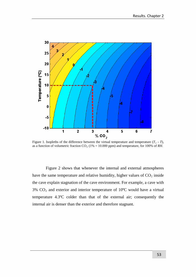
Results. Chapter 2
53
Figure 1. Isopleths of the difference between the virtual temperature and temperature (Tv - T), as a function of volumetric fraction CO2 (1% = 10.000 ppm) and temperature, for 100% of RH.
Figure 2 shows that whenever the internal and external atmospheres
have the same temperature and relative humidity, higher values of CO2 inside
the cave explain stagnation of the cave environment. For example, a cave with
3% CO2 and exterior and interior temperature of 10ºC would have a virtual
temperature 4.3ºC colder than that of the external air; consequently the
internal air is denser than the exterior and therefore stagnant.
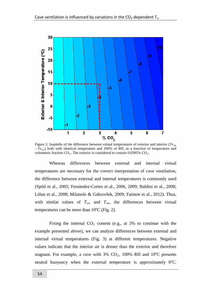
Cave ventilation is influenced by variations in the CO2-dependent Tv.
54
Figure 2. Isopleths of the difference between virtual temperatures of exterior and interior (Tvint - Tvext) both with identical temperature and 100% of RH, as a function of temperature and volumetric fraction CO2. The exterior is considered to contain 0.0395% CO2.
Whereas differences between external and internal virtual
temperatures are necessary for the correct interpretation of cave ventilation,
the difference between external and internal temperatures is commonly used
(Spötl et al., 2005; Fernàndez-Cortes et al., 2006, 2009; Baldini et al., 2008;
Liñan et al., 2008; Milanolo & Gabrovšek, 2009; Faimon et al., 2012). Thus,
with similar values of Text and Tint, the differences between virtual
temperatures can be more than 10ºC (Fig. 2).
Fixing the internal CO2 content (e.g., at 3% to continue with the
example presented above), we can analyze differences between external and
internal virtual temperatures (Fig. 3) at different temperatures. Negative
values indicate that the interior air is denser than the exterior and therefore
stagnant. For example, a cave with 3% CO2, 100% RH and 10ºC presents
neutral buoyancy when the external temperature is approximately 6ºC.
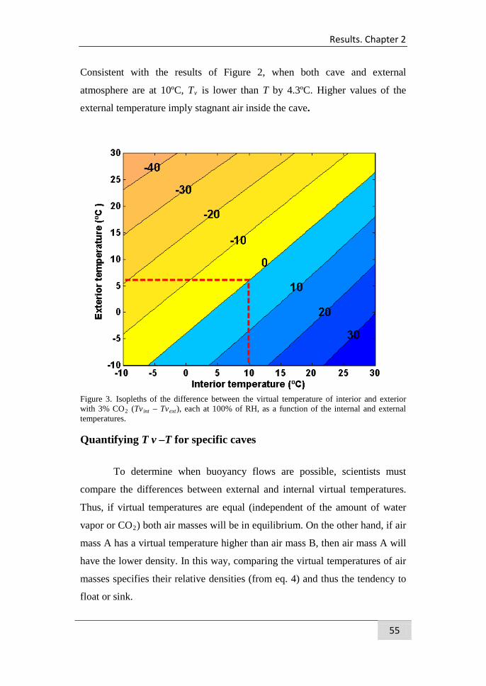
Results. Chapter 2
55
Consistent with the results of Figure 2, when both cave and external
atmosphere are at 10ºC, Tv is lower than T by 4.3ºC. Higher values of the
external temperature imply stagnant air inside the cave.
Figure 3. Isopleths of the difference between the virtual temperature of interior and exterior with 3% CO2 (Tvint – Tvext), each at 100% of RH, as a function of the internal and external temperatures.
Quantifying T v –T for specific caves
To determine when buoyancy flows are possible, scientists must
compare the differences between external and internal virtual temperatures.
Thus, if virtual temperatures are equal (independent of the amount of water
vapor or CO2) both air masses will be in equilibrium. On the other hand, if air
mass A has a virtual temperature higher than air mass B, then air mass A will
have the lower density. In this way, comparing the virtual temperatures of air
masses specifies their relative densities (from eq. 4) and thus the tendency to
float or sink.
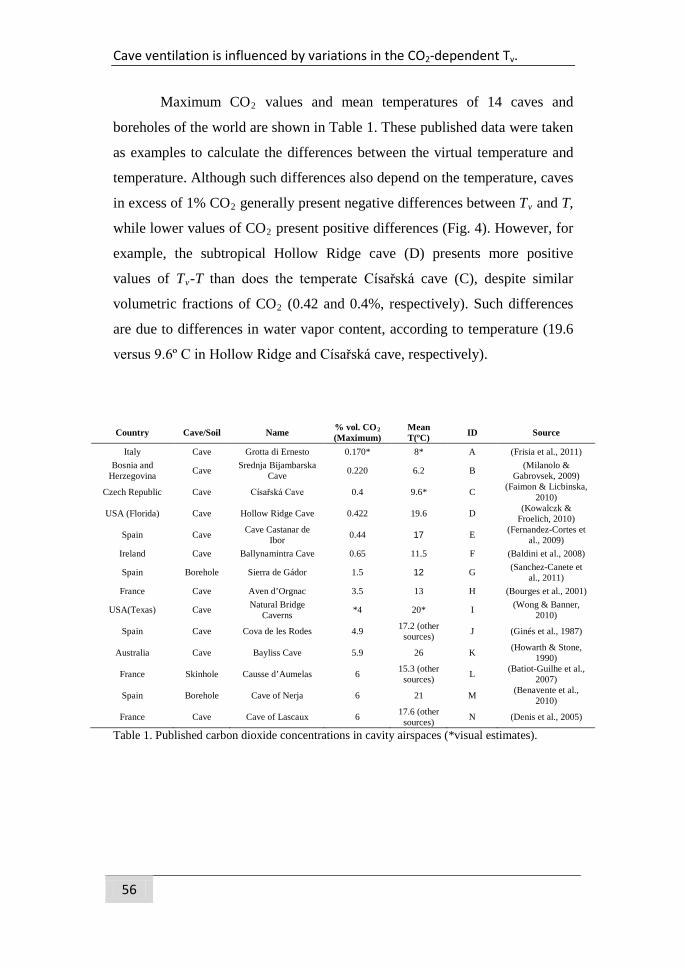
Cave ventilation is influenced by variations in the CO2-dependent Tv.
56
Maximum CO2 values and mean temperatures of 14 caves and
boreholes of the world are shown in Table 1. These published data were taken
as examples to calculate the differences between the virtual temperature and
temperature. Although such differences also depend on the temperature, caves
in excess of 1% CO2 generally present negative differences between Tv and T,
while lower values of CO2 present positive differences (Fig. 4). However, for
example, the subtropical Hollow Ridge cave (D) presents more positive
values of Tv-T than does the temperate Císařská cave (C), despite similar
volumetric fractions of CO2 (0.42 and 0.4%, respectively). Such differences
are due to differences in water vapor content, according to temperature (19.6
versus 9.6º C in Hollow Ridge and Císařská cave, respectively).
Table 1. Published carbon dioxide concentrations in cavity airspaces (*visual estimates).
Country Cave/Soil Name % vol. CO2 (Maximum)
Mean T(ºC) ID Source
Italy Cave Grotta di Ernesto 0.170* 8* A (Frisia et al., 2011) Bosnia and
Herzegovina Cave Srednja Bijambarska Cave 0.220 6.2 B (Milanolo &
Gabrovsek, 2009)
Czech Republic Cave Císařská Cave 0.4 9.6* C (Faimon & Licbinska, 2010)
USA (Florida) Cave Hollow Ridge Cave 0.422 19.6 D (Kowalczk & Froelich, 2010)
Spain Cave Cave Castanar de Ibor 0.44 17 E (Fernandez-Cortes et
al., 2009) Ireland Cave Ballynamintra Cave 0.65 11.5 F (Baldini et al., 2008)
Spain Borehole Sierra de Gádor 1.5 12 G (Sanchez-Canete et al., 2011)
France Cave Aven d’Orgnac 3.5 13 H (Bourges et al., 2001)
USA(Texas) Cave Natural Bridge Caverns *4 20* I (Wong & Banner,
2010)
Spain Cave Cova de les Rodes 4.9 17.2 (other sources) J (Ginés et al., 1987)
Australia Cave Bayliss Cave 5.9 26 K (Howarth & Stone, 1990)
France Skinhole Causse d’Aumelas 6 15.3 (other sources) L (Batiot-Guilhe et al.,
2007)
Spain Borehole Cave of Nerja 6 21 M (Benavente et al., 2010)
France Cave Cave of Lascaux 6 17.6 (other sources) N (Denis et al., 2005)
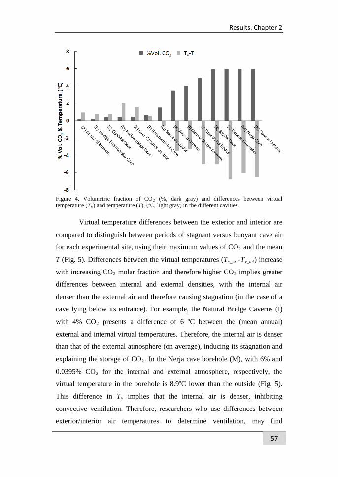
Results. Chapter 2
57
Figure 4. Volumetric fraction of CO2 (%, dark gray) and differences between virtual temperature (Tv) and temperature (T), (ºC, light gray) in the different cavities.
Virtual temperature differences between the exterior and interior are
compared to distinguish between periods of stagnant versus buoyant cave air
for each experimental site, using their maximum values of CO2 and the mean
T (Fig. 5). Differences between the virtual temperatures (Tv_ext-Tv_int) increase
with increasing CO2 molar fraction and therefore higher CO2 implies greater
differences between internal and external densities, with the internal air
denser than the external air and therefore causing stagnation (in the case of a
cave lying below its entrance). For example, the Natural Bridge Caverns (I)
with 4% CO2 presents a difference of 6 ºC between the (mean annual)
external and internal virtual temperatures. Therefore, the internal air is denser
than that of the external atmosphere (on average), inducing its stagnation and
explaining the storage of CO2. In the Nerja cave borehole (M), with 6% and
0.0395% CO2 for the internal and external atmosphere, respectively, the
virtual temperature in the borehole is 8.9ºC lower than the outside (Fig. 5).
This difference in Tv implies that the internal air is denser, inhibiting
convective ventilation. Therefore, researchers who use differences between
exterior/interior air temperatures to determine ventilation, may find
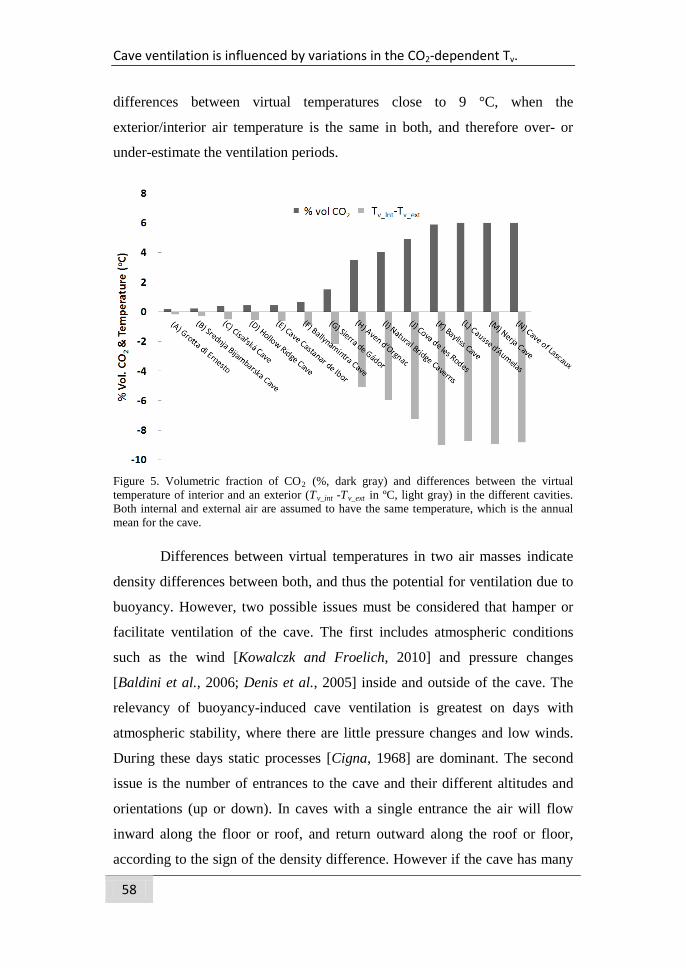
Cave ventilation is influenced by variations in the CO2-dependent Tv.
58
differences between virtual temperatures close to 9 °C, when the
exterior/interior air temperature is the same in both, and therefore over- or
under-estimate the ventilation periods.
Figure 5. Volumetric fraction of CO2 (%, dark gray) and differences between the virtual temperature of interior and an exterior (Tv_int -Tv_ext in ºC, light gray) in the different cavities. Both internal and external air are assumed to have the same temperature, which is the annual mean for the cave.
Differences between virtual temperatures in two air masses indicate
density differences between both, and thus the potential for ventilation due to
buoyancy. However, two possible issues must be considered that hamper or
facilitate ventilation of the cave. The first includes atmospheric conditions
such as the wind [Kowalczk and Froelich, 2010] and pressure changes
[Baldini et al., 2006; Denis et al., 2005] inside and outside of the cave. The
relevancy of buoyancy-induced cave ventilation is greatest on days with
atmospheric stability, where there are little pressure changes and low winds.
During these days static processes [Cigna, 1968] are dominant. The second
issue is the number of entrances to the cave and their different altitudes and
orientations (up or down). In caves with a single entrance the air will flow
inward along the floor or roof, and return outward along the roof or floor,
according to the sign of the density difference. However if the cave has many
Results. Chapter 2
59
entrances at different levels, it may be necessary to monitor more than one
entrance [Cigna, 1968]. Due to the strong spatial variability of the
temperature, simply knowing Tv at a single point inside (and outside) the cave
may not necessarily be sufficient for determining the potential for ventilation.
4.2.4. Conclusions
We used the information of several caves together with gas law to
demonstrate that the difference between external and internal virtual
temperatures including CO2 effects determines the buoyancy and should be
used for the correct interpretation of cave ventilation. Often scientists estimate
ventilation neglecting CO2 effects, but this can cause errors close to 9 °C in
the difference between external and internal virtual temperatures when the air
temperature is the same in both. Thus, the common use of the difference
between external and internal temperatures could over- or under-estimate the
existence of ventilation processes, depending on CO2 content and relative
humidity.
Acknowledgements
This research was funded by the Andalusian regional government
project GEOCARBO (P08-RNM-3721) and GLOCHARID, including
European Union ERDF funds, with support from Spanish Ministry of Science
and Innovation projects Carbored-II (CGL2010-22193-C04-02), SOILPROF
(CGL2011-15276-E) and CARBORAD (CGL2011-27493), as well as the
European Community's Seventh Framework Programme (FP7/2007-2013)
under grant agreement n° 244122. The authors thank three anonymous
reviewers for constructive comments that helped to substantially improve the
manuscript.
Cave ventilation is influenced by variations in the CO2-dependent Tv.
60
Appendix A
The starting point for deriving the virtual temperature is the ideal gas
law:
TnRpV *= (eq. A1)
where p, V, n, R* and T are the pressure (Pa), volume (m3), number of
moles (moles), universal gas constant (8.314 m3 Pa K-1 mol-1) and absolute
temperature (K) of the gas, respectively. Since the number of moles (n) is
equal to the mass (m, in kg) divided by the molar mass (M, in kg mol-1),
equation 1 can be written as:
TRMmpV *= (eq. A2)
By substituting the density, Vm=ρ this can be rewritten in the
form:
TMRp
*
ρ=
(eq. A3)
When defining the particular gas constant (R) as MRR *= , the
equation of state for the atmosphere can be written in the form convenient for
meteorologists as:
RTp ρ= (eq. A4)
where p, ρ, R and T are the pressure (Pa=J m-3), density (kg m-3), particular
gas constant (J kg-1 K-1) and absolute temperature (K) of the gas, respectively.
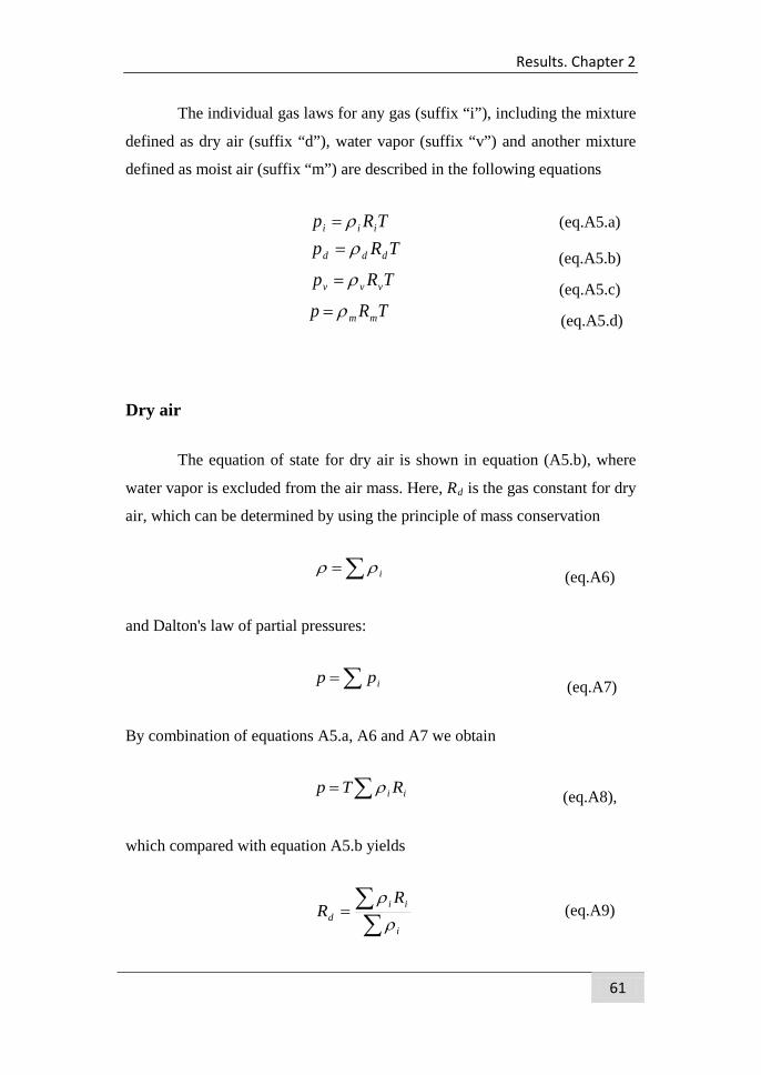
Results. Chapter 2
61
The individual gas laws for any gas (suffix “i”), including the mixture
defined as dry air (suffix “d”), water vapor (suffix “v”) and another mixture
defined as moist air (suffix “m”) are described in the following equations
TRp iii ρ= (eq.A5.a)
TRp ddd ρ= (eq.A5.b) TRp vvv ρ= (eq.A5.c)
TRp mmρ= (eq.A5.d)
Dry air
The equation of state for dry air is shown in equation (A5.b), where
water vapor is excluded from the air mass. Here, Rd is the gas constant for dry
air, which can be determined by using the principle of mass conservation
∑= iρρ (eq.A6)
and Dalton's law of partial pressures:
∑= ipp (eq.A7)
By combination of equations A5.a, A6 and A7 we obtain
∑= ii RTp ρ (eq.A8),
which compared with equation A5.b yields
∑∑=
i
iid
RR
ρρ
(eq.A9)
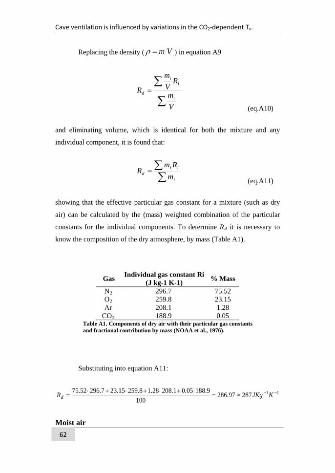
Cave ventilation is influenced by variations in the CO2-dependent Tv.
62
Replacing the density ( Vm=ρ ) in equation A9
∑
∑=
Vm
RVm
Ri
ii
d
(eq.A10)
and eliminating volume, which is identical for both the mixture and any
individual component, it is found that:
∑∑=
i
iid m
RmR
(eq.A11)
showing that the effective particular gas constant for a mixture (such as dry
air) can be calculated by the (mass) weighted combination of the particular
constants for the individual components. To determine Rd it is necessary to
know the composition of the dry atmosphere, by mass (Table A1).
Gas Individual gas constant Ri (J kg-1 K-1) % Mass
N2 296.7 75.52 O2 259.8 23.15 Ar 208.1 1.28
CO2 188.9 0.05 Table A1. Components of dry air with their particular gas constants and fractional contribution by mass (NOAA et al., 1976).
Substituting into equation A11:
1128797.286100
9.18805.01.20828.18.25915.237.29652.75 −−≅=⋅+⋅+⋅+⋅
= KJKgRd
Moist air
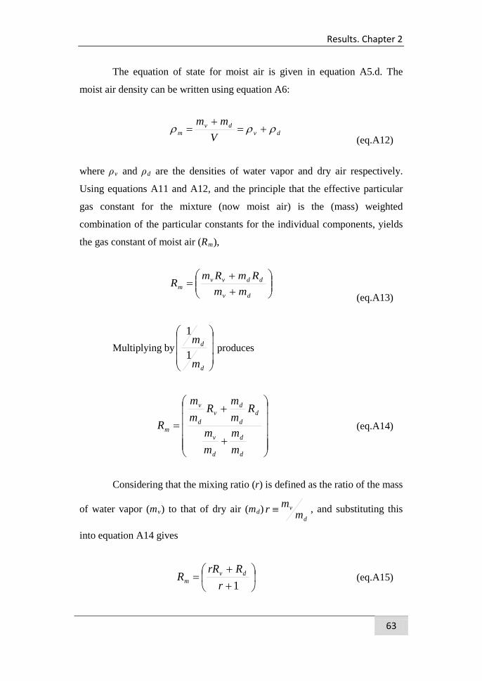
Results. Chapter 2
63
The equation of state for moist air is given in equation A5.d. The
moist air density can be written using equation A6:
dvdv
m Vmm
ρρρ +=+
= (eq.A12)
where ρv and ρd are the densities of water vapor and dry air respectively.
Using equations A11 and A12, and the principle that the effective particular
gas constant for the mixture (now moist air) is the (mass) weighted
combination of the particular constants for the individual components, yields
the gas constant of moist air (Rm),
++
=dv
ddvvm mm
RmRmR
(eq.A13)
Multiplying by
d
d
m
m1
1 produces
+
+=
d
d
d
v
dd
dv
d
v
m
mm
mm
Rmm
Rmm
R
(eq.A14)
Considering that the mixing ratio (r) is defined as the ratio of the mass
of water vapor (mv) to that of dry air (md)d
vm
mr ≡ , and substituting this
into equation A14 gives
++
=1rRrR
R dvm
(eq.A15)
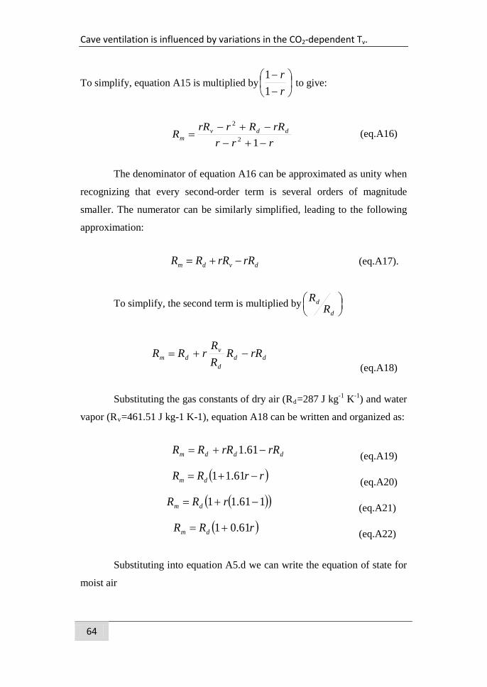
Cave ventilation is influenced by variations in the CO2-dependent Tv.
64
To simplify, equation A15 is multiplied by
−−
rr
11
to give:
rrrrRRrrR
R ddvm −+−
−+−=
12
2
(eq.A16)
The denominator of equation A16 can be approximated as unity when
recognizing that every second-order term is several orders of magnitude
smaller. The numerator can be similarly simplified, leading to the following
approximation:
dvdm rRrRRR −+= (eq.A17).
To simplify, the second term is multiplied by
d
dR
R
ddd
vdm rRR
RR
rRR −+= (eq.A18)
Substituting the gas constants of dry air (Rd=287 J kg-1 K-1) and water
vapor (Rv=461.51 J kg-1 K-1), equation A18 can be written and organized as:
dddm rRrRRR −+= 61.1 (eq.A19)
( )rrRR dm −+= 61.11 (eq.A20)
( )( )161.11 −+= rRR dm (eq.A21)
( )rRR dm 61.01 += (eq.A22)
Substituting into equation A5.d we can write the equation of state for
moist air
Results. Chapter 2
65
( )TrRp dm 61.01 += ρ (eq.A23)
Rather than associating the varying water vapor effect (1+0.61r) with the gas
constant (and thus producing a variable constant), meteorologists traditionally
associate this term with the temperature. Thus, through equation A23, the
virtual temperature for the atmosphere is defined as:
)61.01( rTTv += (eq.A24)
CO2 rich-air
Equations to calculate the virtual temperature including CO2 effects
were developed by Kowalski & Sanchez-Cañete (2010). An approximation to
calculate the virtual temperature (Tv) including CO2 effects is via the
following equation:
)3419.06079.01( cvv rrTT −+= (eq.A25)
where Tv is the virtual temperature (K), and rv and rc are the water vapour and
carbon dioxide mixing ratios respectively (dimensionless).
The errors when using equation A25 as an approximation to Tv
(including CO2 effects) were evaluated explicitly for the range of gas
concentrations typically found in terrestrial caves and found to be less than
0.1% (0.3 K) for volumetric CO2 fractions of up to 5%.
For a calculation without error, the virtual temperature should be
defined using the particular gas constant for the mixture of moist air including
high concentrations of CO2, denoted as Rmc and defined as:
Cave ventilation is influenced by variations in the CO2-dependent Tv.
66
vc
vvccnoamc rr
RrRrRR
++++
=1 (eq. A26)
where Rnoa is the particular gas constant for the mixture of nitrogen (N2),
oxygen (O2), and argon (Ar) (287.0 J K-1 kg-3), Rc is the particular gas
constant for CO2 (188.9 J K-1 kg-3), Rv is the particular gas constant for water
vapor (461.5 J K-1 kg-3), rv is the water vapor mixing ratio (dimensionless),
and rc is the carbon dioxide mixing ratio (dimensionless).
The exact expression for Tv is then.
++
++
=noa
vc
vvccnoa
v Rrr
RrRrR
TT1
(eq. A27)
which is programmed in an Excel file freely available at
http://fisicaaplicada.ugr.es/pages/tv/!/download
Therefore for determining air density in caves or soils including CO2
effects, the virtual temperature can be used in the ideal gas law with the
particular gas constant for the mixture of nitrogen (N2), oxygen (O2), and
argon (Ar)
vnoa TRp ⋅⋅= ρ (eq.A28).
Results. Chapter 2
67
References Amundson, R. G., and E. A. Davidson (1990), Carbon dioxide and
nitrogenous gases in the soil atmosphere, J. Geochem. Explor., 38(1-
2), 13-41.
Atkinson, T. C. (1977), Carbon-dioxide in atmosphere of unsaturated zone -
important control of groundwater hardness in limestones., J. Hydrol.,
35(1-2), 111-123.
Badino, G., J. M. Calaforra, P. Forti, P. Garofalo, and L. Sanna (2011), The
present day genesis and evolution of cave minerals inside the Ojo de
la Reina Cave (Naica Mine, Mexico), Int. J. Speleol., 40(2), 125-131.
Baldini, J. U. L., L. M. Baldini, F. McDermott, and N. Clipson (2006),
Carbon dioxide sources, sinks, and spatial variability in shallow
temperate zone caves: Evidence from Ballynamintra Cave, Ireland, J.
Cave Karst Stud., 68(1), 4-11.
Baldini, J. U. L., F. McDermott, D. L. Hoffmann, D. A. Richards, and N.
Clipson (2008), Very high-frequency and seasonal cave atmosphere
P(CO2) variability: Implications for stalagmite growth and oxygen
isotope-based paleoclimate records, Earth Planet. Sci. Lett., 272(1-2),
118-129.
Banner, J. L., A. Guilfoyle, E. W. James, L. A. Stern, and M. Musgrove
(2007), Seasonal variations in modern speleothem calcite growth in
Central Texas, USA, J. Sediment. Res., 77(7-8), 615-622.
Batiot-Guilhe, C., J. L. Seidel, H. Jourde, O. Hebrard, and V. Bailly-Comte
(2007), Seasonal variations of CO2 and Rn222 in a mediterranean
sinkhole - spring (Causse d'Aumelas, SE France), Int. J. Speleol.,
36(1), 51-56.
Benavente, J., I. Vadillo, F. Carrasco, A. Soler, C. Linan, and F. Moral
(2010), Air Carbon Dioxide Contents in the Vadose Zone of a
Mediterranean Karst, Vadose Zone J., 9(1), 126-136.
Cave ventilation is influenced by variations in the CO2-dependent Tv.
68
Bourges, F., A. Mangin, and D. d'Hulst (2001), Carbon dioxide in karst cavity
atmosphere dynamics: the example of the Aven d'Orgnac (Ardeche),
Comptes Rendus Acad. Sci. Ser II-A, 333(11), 685-692.
Bourges, F., P. Genthon, D. Genty, A. Mangin, and D. D'Hulst (2012),
Comment on "Carbon uptake by karsts in the Houzhai Basin,
southwest China" by Junhua Yan et al, J. Geophys. Res.-Biogeosci.,
117.
Cigna A.A., 1968 - An analytical study of air circulation in caves.
International Journal of Speleology, 3: 41-54.
De Freitas C. R., Littlejohn R. N., Clarkson T. S. & Kristament I. S., 1982 -
Cave climate: Assessment of airf low and ventilation. Journal of
Climatology, 2: 383-397.
Denis, A., R. Lastennet, F. Huneau, and P. Malaurent (2005), Identification of
functional relationships between atmospheric pressure and CO2 in the
cave of Lascaux using the concept of entropy of curves, Geophys.
Res. Lett., 32(5).
Ek, C., and M. Gewelt (1985), Carbon dioxide in cave atmospheres. New
results in Belgium and comparison with some other countries., Earth
Surf. Process. Landf., 10(2), 173-187.
Faimon, J., J. Stelcl, and D. Sas (2006), Anthropogenic CO2-flux into cave
atmosphere and its environmental impact: A case study in the
Cisarska Cave (Moravian Karst, Czech Republic), Science of the
Total Environment, 369(1-3), 231-245.
Faimon, J., D. Troppova, V. Baldik, and R. Novotny (2012), Air circulation
and its impact on microclimatic variables in the Cisarska Cave
(Moravian Karst, Czech Republic), Int. J. Climatol., 32(4), 599-623.
Fairchild, I. J., and A. Baker (2012), Speleothem Science: from process to past
environments, Wiley-Blackwell.
Fernandez-Cortes, A., J. M. Calaforra, and F. Sanchez-Martos (2006),
Spatiotemporal analysis of air conditions as a tool for the
Results. Chapter 2
69
environmental management of a show cave (Cueva del Agua, Spain),
Atmospheric Environment, 40(38), 7378-7394.
Fernández-Cortes A., Sanchez-Moral S., Cuezva S., Cañaveras J. C. & Abella
R., (2009), Annual and transient signatures of gas exchange and
transport in the Castanar de Ibor cave (Spain). International Journal
of Speleology, 38: 153-162.
Fernández, P. L., I. Gutierrez, L. S. Quindós, J. Soto, and E. Villar (1986),
Natural ventilation of the Paintings Room in the Altamira cave,
Nature, 321(5), 586-588.
Frisia S., Fairchild I. J., Fohlmeister J., Miorandi R., Spötl C. & Borsato A.,
(2011), Carbon mass-balance modelling and carbon isotope exchange
processes in dynamic caves. Geochimica Et Cosmochimica Acta, 75:
380-400.
Ginés A., Hernández J., Ginés J. & Pol A., (1987), Observaciones sobre la
concentración de dióxido de carbono en la Atmósfera de la Cova de
les Rodes. Endins, 13: 27-38.
Hakl, J., I. Hunyadi, I. Csige, G. Geczy, L. Lenart, and A. Varhegyi (1997),
Radon transport phenomena studied in karst caves - International
experiences on radon levels and exposures, Radiat. Meas., 28(1-6),
675-684.
Howarth, F. G., and F. D. Stone (1990), Elevated carbon dioxide levels in
Bayliss Cave, Australia: implications for the evolution of obligate
cave species., Pacific Science, 44(3), 207-218.
Jobbagy, E. G., and R. B. Jackson (2000), The vertical distribution of soil
organic carbon and its relation to climate and vegetation, Ecol. Appl.,
10(2), 423-436.
Keeling, C. D. (1960), The concentration and isotopic abundance of carbon
dioxide in the atmosphere., Tellus, 12(2), 200-203.
Kowalczk, A. J., and P. N. Froelich (2010), Cave air ventilation and CO2
outgassing by radon-222 modeling: How fast do caves breathe?, Earth
Planet. Sci. Lett., 289(1-2), 209-219.
Cave ventilation is influenced by variations in the CO2-dependent Tv.
70
Kowalski, A. S., and E. P. Sanchez-Canete (2010), A New Definition of the
Virtual Temperature, Valid for the Atmosphere and the CO2-Rich Air
of the Vadose Zone, Journal of Applied Meteorology and
Climatology, 49(8), 1692-1695.
Kuzyakov, Y. (2006), Sources of CO2 efflux from soil and review of
partitioning methods, Soil Biol. Biochem., 38(3), 425-448.
Linan, C., I. Vadillo, and F. Carrasco (2008), Carbon dioxide concentration in
air within the Nerja Cave (Malaga, Andalusia, Spain), Int. J. Speleol.,
37(2), 99-106.
Milanolo, S., and F. Gabrovsek (2009), Analysis of Carbon Dioxide
Variations in the Atmosphere of Srednja Bijambarska Cave, Bosnia
and Herzegovina, Bound.-Layer Meteor., 131(3), 479-493.
Nachshon, U., M. Dragila, and N. Weisbrod (2012), From atmospheric winds
to fracture ventilation: Cause and effect, J. Geophys. Res.-Biogeosci.,
117.
NOAA, 1976. U. S. Standard Atmosphere, 1976. NASA and USAF.
Sanchez-Canete, E. P., P. Serrano-Ortiz, A. S. Kowalski, C. Oyonarte, and F.
Domingo (2011), Subterranean CO2 ventilation and its role in the net
ecosystem carbon balance of a karstic shrubland, Geophys. Res. Lett.,
38, L09802.
Schlesinger, W. H. (1997), Biogeochemistry: An Analysis of Global Change,
2 ed., 588 pp., Academic Press, San Diego.
Serrano-Ortiz, P., M. Roland, S. Sanchez-Moral, I. A. Janssens, F. Domingo,
Y. Godderis, and A. S. Kowalski (2010), Hidden, abiotic CO2 flows
and gaseous reservoirs in the terrestrial carbon cycle: Review and
perspectives, Agric. For. Meteorol., 150(3), 321-329.
Spotl, C., I. J. Fairchild, and A. F. Tooth (2005), Cave air control on dripwater
geochemistry, Obir Caves (Austria): Implications for speleothem
deposition in dynamically ventilated caves, Geochim. Cosmochim.
Acta, 69(10), 2451-2468.

Results. Chapter 2
71
Stull R. B., (1988). An introduction to Boundary Layer Meteorology. Kluwer
Academic Publishers, Dordrecht, The Netherlands, 667p.
Weisbrod, N., M. I. Dragila, U. Nachshon, and M. Pillersdorf (2009), Falling
through the cracks: The role of fractures in Earth-atmosphere gas
exchange, Geophys. Res. Lett., 36.

Cave ventilation is influenced by variations in the CO2-dependent Tv.
72
Results.Chapter 3
73
4.3 Chapter 3
Subterranean CO2 ventilation and its role in the net ecosystem carbon balance of a karstic shrubland
Sanchez-Cañete, E.P.1,2 Serrano-Ortiz, P. 1,2 Kowalski, A.S.2,3 Oyonarte, C.4 Domingo, F.1,5
Published in Geophysical Research Letters
Sanchez-Canete, E. P., P. Serrano-Ortiz, A. S. Kowalski, C. Oyonarte, and F. Domingo (2011), Subterranean CO2 ventilation and its role in the net ecosystem carbon balance of a karstic shrubland, Geophysical Research Letteres, 38, L09802.
Subterranean CO2 ventilation and its role in the NECB of a karstic shrubland.
74
Abstract
Recent studies of carbonate ecosystems suggest a possible
contribution of subterranean ventilation to the net ecosystem carbon balance.
However, both the overall importance of such CO2 exchange processes and
their drivers remain unknown. Here we analyze several dry-season episodes
of net CO2 emissions to the atmosphere, along with soil and borehole CO2
measurements. Results highlight important events where rapid decreases of
underground CO2 molar fractions correlate well with sizeable CO2 release to
the atmosphere. Such events, with high friction velocities, are attributed to
ventilation processes, and should be accounted for by predictive models of
surface CO2 exchange.
Results.Chapter 3
75
4.3.1. Introduction
The FLUXNET community monitors ecosystem carbon exchanges,
usually interpreting CO2 fluxes as biological (photosynthetic or respiratory)
[Falge et al., 2002; Reichstein et al., 2005], neglecting inorganic processes.
However, recent studies over carbonate substrates reveal possible
contributions by abiotic processes to the net ecosystem carbon balance
(NECB;[Chapin et al., 2006]), with relevant magnitudes at least on short time
scales [Serrano-Ortiz et al., 2010; Were et al., 2010]. These processes can
temporally dominate the NECB in areas with carbonate soils [Kowalski et al.,
2008].
Carbonates outcrop on ca. 12-18% of the water-free Earth [Ford and
Williams, 1989] with an enormous capacity to store CO2 below ground in
macropores (caves) and fissures [Benavente et al., 2010; Ek and Gewelt,
1985]. Ventilation is a mass flow of air through a cavity, via the porous media
in the case of closed caves, driven by an imbalance of forces (pressure
gradients and gravity). Through the venting of these subterranean spaces,
stored gaseous CO2 can be lost to the atmosphere [Kowalczk and Froelich,
2010; Weisbrod et al., 2009]. However, both the drivers of these ventilation
processes and their relevance to regional CO2 budgets remain unknown.
Often ecologists estimate soil CO2 effluxes neglecting advective
transport of CO2 through the vadose zone. Studies of surface exchange have
usually been conducted either by manual [Janssens et al., 2001], or automatic
soil respiration chambers [Drewitt et al., 2002]. Scientists often model
underground, diffusive soil CO2 fluxes based on single sampling [Davidson
and Trumbore, 1995; Hirsch et al., 2002] or continuous monitoring of CO2
profiles [Baldocchi et al., 2006; Pumpanen et al., 2008; Tang et al., 2003].
Such models based on diffusion processes neglect the effects of ventilation.
However, Subke et al. [2003] revealed the importance of such effects at least
on short-time scales.
Subterranean CO2 ventilation and its role in the NECB of a karstic shrubland.
76
Here we analyze several episodes of subterranean CO2 ventilation
that occurred during a dry period in a carbonate ecosystem. We examine its
determinants and implications for the NECB measured with an eddy
covariance system.
4.3.2. Material and Methods
The study site is El Llano de los Juanes, a shrubland plateau at 1600
m altitude in the Sierra de Gádor (Almería, Southeast Spain; 36º55’41.7’’N;
2º45’1.7’’W). It is characterized by a sub-humid climate with a mean annual
temperature (T) of 12 ºC and precipitation of ca. 465 mm. The soil, overlying
Triassic carbonate rocks, varies from 0 to 150 cm depth with a petrocalcic
horizon and fractured rocks. More detailed site information is given by
Serrano-Ortiz et al.[2009].
Throughout the dry season of 2009 (9 June - 9 September) two
sensors (GMP-343, Vaisala, Inc., Finland) that measure CO2 molar fraction
(χc), were installed in the soil and in a borehole. The soil sensor was installed
25 cm deep, with a soil T probe (107, Campbell scientific, Logan, UT, USA;
hereafter CSI) and water content reflectometer (CS616, CSI). The 7-m
borehole (dia. 0.1 m) was sealed from the atmosphere with a metal tube
cemented to the walls. Inside, sensors tracked χc (GMP-343), radon (Barasol
MC BT45N, Bessines Sur Gartempe, France) and T and relative humidity
(HMP45, CSI). The CO2 sensors were corrected for variations in T and
pressure. A data-logger (CR23X, CSI) measured every 30 s and stored 5 min
averages. Ecosystem-scale CO2 fluxes were measured by eddy covariance
atop a 2.5 m tower; Serrano-Ortiz et al., [2009] describe the instrumentation
and quality control for eddy flux data.
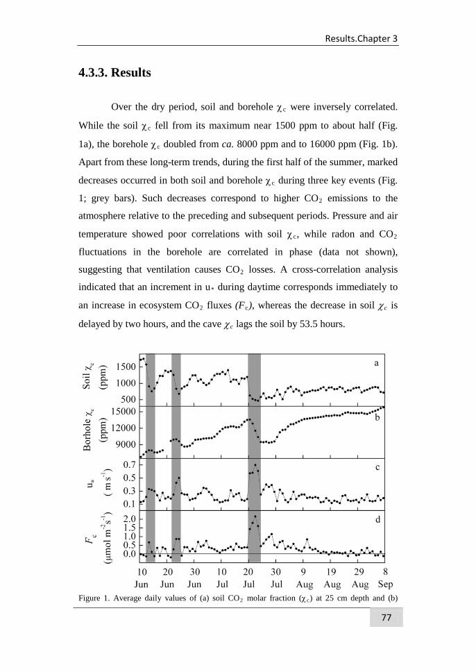
Results.Chapter 3
77
4.3.3. Results
Over the dry period, soil and borehole χc were inversely correlated.
While the soil χc fell from its maximum near 1500 ppm to about half (Fig.
1a), the borehole χc doubled from ca. 8000 ppm and to 16000 ppm (Fig. 1b).
Apart from these long-term trends, during the first half of the summer, marked
decreases occurred in both soil and borehole χc during three key events (Fig.
1; grey bars). Such decreases correspond to higher CO2 emissions to the
atmosphere relative to the preceding and subsequent periods. Pressure and air
temperature showed poor correlations with soil χc, while radon and CO2
fluctuations in the borehole are correlated in phase (data not shown),
suggesting that ventilation causes CO2 losses. A cross-correlation analysis
indicated that an increment in u* during daytime corresponds immediately to
an increase in ecosystem CO2 fluxes (Fc), whereas the decrease in soil χc is
delayed by two hours, and the cave χc lags the soil by 53.5 hours.
Figure 1. Average daily values of (a) soil CO2 molar fraction (χc) at 25 cm depth and (b)
Subterranean CO2 ventilation and its role in the NECB of a karstic shrubland.
78
borehole χc at 7 m depth, (c) friction velocity (u*; turbulent velocity scale) and (d) ecosystem CO2 fluxes (FC; negative values represent uptake). Shaded columns delimit ventilation events.
These events occurred when the friction velocity (u*) exceeded 0.3 m
s-1 (Fig. 1c), and are associated with ventilation. The largest event occurred
during a windy period from July 21st-24th (daily mean u*>0.6 m s-1), when soil
CO2 more than halved from 1200 to 500 ppm and the borehole lost ca. 4000
ppm. This underground CO2 loss corresponded to increased emissions to the
atmosphere of 0.4 - 2 µmol m-2 s-1 (Fig. 1d). After the event, the borehole χc
recovered to exceed initial values (>14000 ppm) within a couple of weeks.
The 21-24 July ventilation event (3rd grey bar, Fig. 1) is detailed in Figure 2,
showing 11 days of half-hour values divided into periods of recharge and
ventilation. During recharge, the borehole χc increased slightly, then fell
quickly during ventilation, losing ca. 4000 ppm in five days (Fig. 2b). Soil
CO2 followed a daily cycle, with late afternoon peaks and dawn minima (Fig.
2a). During recharge, diurnal ranges averaged ca. 800 ppm, versus just 200
ppm during ventilation. The mean soil χc and u* were higher (Fig. 2c) for the
ventilated period. Finally, Fc was near zero with little diurnal variation during
recharge, but daytime emissions exceeded 5 µmol m-2 s-1 during the ventilated
period. At night, CO2 emissions were always close to zero (Fig. 2d).
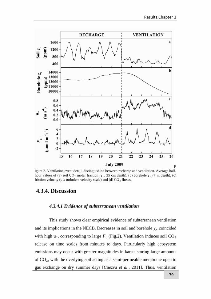
Results.Chapter 3
79
Figure 2. Ventilation event detail, distinguishing between recharge and ventilation. Average half-hour values of (a) soil CO2 molar fraction (χc, 25 cm depth), (b) borehole χc (7 m depth), (c) friction velocity (u*; turbulent velocity scale) and (d) CO2 fluxes.
4.3.4. Discussion
4.3.4.1 Evidence of subterranean ventilation
This study shows clear empirical evidence of subterranean ventilation
and its implications in the NECB. Decreases in soil and borehole χc coincided
with high u*, corresponding to large Fc (Fig.2). Ventilation induces soil CO2
release on time scales from minutes to days. Particularly high ecosystem
emissions may occur with greater magnitudes in karsts storing large amounts
of CO2, with the overlying soil acting as a semi-permeable membrane open to
gas exchange on dry summer days [Cuezva et al., 2011]. Thus, ventilation
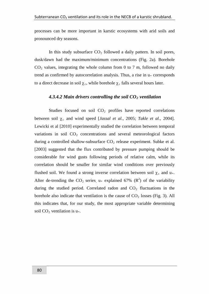
Subterranean CO2 ventilation and its role in the NECB of a karstic shrubland.
80
processes can be more important in karstic ecosystems with arid soils and
pronounced dry seasons.
In this study subsurface CO2 followed a daily pattern. In soil pores,
dusk/dawn had the maximum/minimum concentrations (Fig. 2a). Borehole
CO2 values, integrating the whole column from 0 to 7 m, followed no daily
trend as confirmed by autocorrelation analysis. Thus, a rise in u* corresponds
to a direct decrease in soil χc, while borehole χc falls several hours later.
4.3.4.2 Main drivers controlling the soil CO2 ventilation
Studies focused on soil CO2 profiles have reported correlations
between soil χc and wind speed [Jassal et al., 2005; Takle et al., 2004].
Lewicki et al [2010] experimentally studied the correlation between temporal
variations in soil CO2 concentrations and several meteorological factors
during a controlled shallow-subsurface CO2 release experiment. Subke et al.
[2003] suggested that the flux contributed by pressure pumping should be
considerable for wind gusts following periods of relative calm, while its
correlation should be smaller for similar wind conditions over previously
flushed soil. We found a strong inverse correlation between soil χc and u*.
After de-trending the CO2 series, u* explained 67% (R2) of the variability
during the studied period. Correlated radon and CO2 fluctuations in the
borehole also indicate that ventilation is the cause of CO2 losses (Fig. 3). All
this indicates that, for our study, the most appropriate variable determining
soil CO2 ventilation is u*.
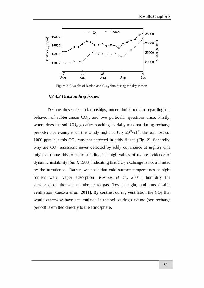
Results.Chapter 3
81
Figure 3. 3 weeks of Radon and CO2 data during the dry season.
4.3.4.3 Outstanding issues
Despite these clear relationships, uncertainties remain regarding the
behavior of subterranean CO2, and two particular questions arise. Firstly,
where does the soil CO2 go after reaching its daily maxima during recharge
periods? For example, on the windy night of July 20th-21st, the soil lost ca.
1000 ppm but this CO2 was not detected in eddy fluxes (Fig. 2). Secondly,
why are CO2 emissions never detected by eddy covariance at nights? One
might attribute this to static stability, but high values of u* are evidence of
dynamic instability [Stull, 1988] indicating that CO2 exchange is not a limited
by the turbulence. Rather, we posit that cold surface temperatures at night
foment water vapor adsorption [Kosmas et al., 2001], humidify the
surface, close the soil membrane to gas flow at night, and thus disable
ventilation [Cuezva et al., 2011]. By contrast during ventilation the CO2 that
would otherwise have accumulated in the soil during daytime (see recharge
period) is emitted directly to the atmosphere.
Subterranean CO2 ventilation and its role in the NECB of a karstic shrubland.
82
4.3.5. Conclusions
This study emphasizes the role of dry-season, subterranean ventilation
processes in the net ecosystem carbon balance (NECB). Although several
meteorological factors correlate with emitted CO2, analyses suggest that
ventilation is driven mainly by the friction velocity. Windy days are
responsible for large emissions of CO2 previously accumulated below ground,
which are not accounted for in current models of surface CO2 exchange.
However during calm days soil CO2 accumulates, causing significant day-
night concentration differences. The vast network of pores, cracks and cavities
along with high molar fractions (>15000ppm-7m) indicate that very large
amounts of CO2 can be stored inside karst systems. Further investigation is
needed to explain the absence of CO2 ventilation during windy nights, and
characterize the CO2 cycling of carbonate ecosystems.
Acknowledgements
This research was funded by the Andalusian regional government
projects GEOCARBO (P08-RNM-3721) and GLOCHARID, including
European Union ERDF funds, with support from European Community's
Seventh Framework Programme (FP7/2007-2013) under grant agreement n°
244122 and Spanish Ministry of Science and Innovation projects PROBASE
(CGL2006-11619/HID) and (Carbored-II; CGL2010-22193-C04-02).
Comments from Jukka Pumpanen and two anonymous referees improved this
manuscript.
Results.Chapter 3
83
References Baldocchi, D., J. W. Tang, and L. K. Xu (2006), How switches and lags in
biophysical regulators affect spatial-temporal variation of soil
respiration in an oak-grass savanna, J. Geophys. Res.-Biogeosci.,
111(G2).
Benavente, J., I. Vadillo, F. Carrasco, A. Soler, C. Linan, and F. Moral
(2010), Air Carbon Dioxide Contents in the Vadose Zone of a
Mediterranean Karst, Vadose Zone J., 9(1), 126-136.
Chapin, F. S., et al. (2006), Reconciling carbon-cycle concepts, terminology,
and methods, Ecosystems, 9(7), 1041-1050.
Cuezva, S., A. Fernandez-Cortes, D. Benavente, P. Serrano-Ortiz, A. S.
Kowalski, and S. Sanchez-Moral (2011), Short-term CO2(g) exchange
between a shallow karstic cavity and the external atmosphere during
summer: Role of the surface soil layer, Atmospheric Environment,
45(7), 1418-1427.
Davidson, E. A., and S. E. Trumbore (1995), Gas diffusivity and production
of CO2 in deep soils of the eastern Amazon, Tellus Ser. B-Chem.
Phys. Meteorol., 47(5), 550-565.
Drewitt, G. B., T. A. Black, Z. Nesic, E. R. Humphreys, E. M. Jork, R.
Swanson, G. J. Ethier, T. Griffis, and K. Morgenstern (2002),
Measuring forest floor CO2 fluxes in a Douglas-fir forest, Agric. For.
Meteorol., 110(4), 299-317.
Ek, C., and M. Gewelt (1985), Carbon dioxide in cave atmospheres. New
results in Belgium and comparison with some other countries., Earth
Surf. Process. Landf., 10(2), 173-187.
Falge, E., et al. (2002), Seasonality of ecosystem respiration and gross
primary production as derived from FLUXNET measurements, Agric.
For. Meteorol., 113(1-4), 53-74.
Ford, D. C., and P. W. Williams (1989), Karst Geomorphology and
Hydrology, 601 pp., London.
Subterranean CO2 ventilation and its role in the NECB of a karstic shrubland.
84
Hirsch, A. I., S. E. Trumbore, and M. L. Goulden (2002), Direct measurement
of the deep soil respiration accompanying seasonal thawing of a
boreal forest soil, J. Geophys. Res.-Atmos., 108(D3).
Janssens, I. A., A. S. Kowalski, and R. Ceulemans (2001), Forest floor CO2
fluxes estimated by eddy covariance and chamber-based model,
Agric. For. Meteorol., 106(1), 61-69.
Jassal, R., A. Black, M. Novak, K. Morgenstern, Z. Nesic, and D. Gaumont-
Guay (2005), Relationship between soil CO2 concentrations and
forest-floor CO2 effluxes, Agric. For. Meteorol., 130(3-4), 176-192.
Kosmas, C., M. Marathianou, S. Gerontidis, V. Detsis, M. Tsara, and J.
Poesen (2001), Parameters affecting water vapor adsorption by the
soil under semi-arid climatic conditions, Agric. Water Manage.,
48(1), 61-78.
Kowalczk, A. J., and P. N. Froelich (2010), Cave air ventilation and CO2
outgassing by radon-222 modeling: How fast do caves breathe?, Earth
Planet. Sci. Lett., 289(1-2), 209-219.
Kowalski, A. S., P. Serrano-Ortiz, I. A. Janssens, S. Sanchez-Moraic, S.
Cuezva, F. Domingo, A. Were, and L. Alados-Arboledas (2008), Can
flux tower research neglect geochemical CO2 exchange?, Agric. For.
Meteorol., 148(6-7), 1045-1054.
Lewicki, J. L., G. E. Hilley, L. Dobeck, and L. Spangler (2010), Dynamics of
CO2 fluxes and concentrations during a shallow subsurface CO2
release, Environ. Earth Sci., 60(2), 285-297.
Pumpanen, J., H. Ilvesniemi, L. Kulmala, E. Siivola, H. Laakso, P. Kolari, C.
Helenelund, M. Laakso, M. Uusimaa, and P. Hari (2008), Respiration
in boreal forest soil as determined from carbon dioxide concentration
profile, Soil Sci. Soc. Am. J., 72(5), 1187-1196.
Reichstein, M., et al. (2005), On the separation of net ecosystem exchange
into assimilation and ecosystem respiration: review and improved
algorithm, Glob. Change Biol., 11(9), 1424-1439.
Results.Chapter 3
85
Serrano-Ortiz, P., M. Roland, S. Sanchez-Moral, I. A. Janssens, F. Domingo,
Y. Godderis, and A. S. Kowalski (2010), Hidden, abiotic CO2 flows
and gaseous reservoirs in the terrestrial carbon cycle: Review and
perspectives, Agric. For. Meteorol., 150(3), 321-329.
Serrano-Ortiz, P., F. Domingo, A. Cazorla, A. Were, S. Cuezva, L.
Villagarcia, L. Alados-Arboledas, and A. S. Kowalski (2009),
Interannual CO2 exchange of a sparse Mediterranean shrubland on a
carbonaceous substrate, J. Geophys. Res.-Biogeosci., 114, G04015.
Stull, R. B. (1988), An introduction to Boundary Layer Meteorology, 667 pp.,
Kluwer Academic Publishers, Dordrecht, The Netherlands.
Subke, J. A., M. Reichstein, and J. D. Tenhunen (2003), Explaining temporal
variation in soil CO2 efflux in a mature spruce forest in Southern
Germany, Soil Biol. Biochem., 35(11), 1467-1483.
Takle, E. S., W. J. Massman, J. R. Brandle, R. A. Schmidt, X. H. Zhou, I. V.
Litvina, R. Garcia, G. Doyle, and C. W. Rice (2004), Influence of
high-frequency ambient pressure pumping on carbon dioxide efflux
from soil, Agric. For. Meteorol., 124(3-4), 193-206.
Tang, J. W., D. D. Baldocchi, Y. Qi, and L. K. Xu (2003), Assessing soil CO2
efflux using continuous measurements of CO2 profiles in soils with
small solid-state sensors, Agric. For. Meteorol., 118(3-4), 207-220.
Weisbrod, N., M. I. Dragila, U. Nachshon, and M. Pillersdorf (2009), Falling
through the cracks: The role of fractures in Earth-atmosphere gas
exchange, Geophys. Res. Lett., 36.
Were, A., P. Serrano-Ortiz, C. M. de Jong, L. Villagarcia, F. Domingo, and A.
S. Kowalski (2010), Ventilation of subterranean CO2 and Eddy
covariance incongruities over carbonate ecosystems, Biogeosciences,
7(3), 859-867.

Subterranean CO2 ventilation and its role in the NECB of a karstic shrubland.
86
Results. Chapter 4
87
4.4 Chapter 4
Deep CO2 soil inhalation/exhalation induced by synoptic pressure changes and atmospheric tides in a
carbonated semiarid steppe
Sánchez-Cañete E.P. 1,2, Kowalski A.S.2,3, Serrano-Ortiz P.1,2, Pérez-Priego O.2,3, Domingo F.1
Published in Biogeosciences Disscusions
Sánchez-Cañete, E. P., Kowalski, A. S., Serrano-Ortiz, P., Pérez-Priego, O., and Domingo, F (2013), Deep CO2 soil inhalation/exhalation induced by synoptic pressure changes and atmospheric tides in a carbonated semiarid steppe, Biogeosciences Discuss., 10, 5591-5618.
Deep CO2 soil fluctuation induced by pressure change.
88
Abstract
Knowledge of all the mechanisms and processes involved in soil CO2
emissions is essential to close the global carbon cycle. Apart from molecular
diffusion, the main physical component of such CO2 exchange is soil
ventilation. Advective CO2 transport, through soil or snow, has been
correlated with the wind speed, friction velocity or pressure (p). Here we
examine variations in subterranean CO2 molar fractions (χc) over two years
within a vertical profile (1.5 m) in a semiarid ecosystem, as influenced by
short-timescale p changes.
Analyses to determine the factors involved in the variations in
subterranean χc were differentiated between the growing period and the dry
period. In both periods it was found that variations in deep χc (0.5 -1.5 m)
were due predominantly to static p variations and not to wind or biological
influences. Within a few hours, the deep χc can vary by fourfold showing a
pattern with two cycles per day, due to p oscillations caused by atmospheric
tides. By contrast, shallow χc (0.15 m) generally has one cycle per day as
influenced by biological factors like soil water content and temperature in
both periods, while the wind was an important factor in shallow χc variations
only during the dry period. Evidence of emissions was registered in the
atmospheric boundary layer by eddy covariance during synoptic pressure
changes when subterranean CO2 was released; days with rising barometric
pressure – when air accumulated belowground, including soil-respired CO2 –
showed greater ecosystem uptake than days with falling pressure. Future
assessments of the net ecosystem carbon balance should not rely exclusively
on Fick's law to calculate soil CO2 effluxes from profile data.
Results. Chapter 4
89
4.4.1. Introduction
The characterization of the different mechanisms and processes
involved in soil CO2 emissions to the atmosphere is important for improving
understanding of the global carbon cycle. Respiration is generally the only
process considered by the FLUXNET community when modeling or
interpreting soil-atmosphere CO2 exchanges [Falge et al., 2002], presumably
transported by molecular diffusion. Recently however, numerous studies of
semiarid ecosystems have shown the importance in the net ecosystem carbon
balance (NECB; [Chapin et al., 2006]) of other, abiotic components
[Emmerich, 2003; Kowalski et al., 2008; Mielnick et al., 2005; Plestenjak et
al., 2012; Rey et al., 2012b; Serrano-Ortiz et al., 2010; Were et al., 2010].
Most researchers interpret soil CO2 effluxes at the soil surface in
terms of concurrent respiration, neglecting subterranean CO2 storage.
Ventilation can decouple the soil CO2 source from emissions to the
atmosphere with changes in pressure, wind or friction velocity. Scientists have
confirmed subterranean advective transport in laboratories [Martin Maier et
al., 2012; Nachshon et al., 2012], soils [M. Maier et al., 2010; Subke et al.,
2003], peatlands [Comas et al., 2005; Comas et al., 2007; Comas et al., 2011],
and snow [Bowling and Massman, 2011; Fujiyoshi et al., 2010; Massman et
al., 1997; Seok et al., 2009]. Some have applied the gradient method - based
on Fick's law for molecular diffusion - to model exchange with the
atmosphere during calm conditions, but highlight the importance of advective
transport in exchanges at other times.
Advective transport of CO2 through soil or snow has been correlated
with changes in subterranean CO2 molar fractions (χc) in conjunction with
variations in wind speed, friction velocity or pressure (p). Advection has been
detected using isotopic methods [Bowling and Massman, 2011], buried p
sensors [M. Maier et al., 2010; Takle et al., 2004], 222Rn concentrations
Deep CO2 soil fluctuation induced by pressure change.
90
[Fujiyoshi et al., 2010], ground penetrating radar [Comas et al., 2005] or
variations in CO2 and other gases [Hirsch et al., 2004; Reicosky et al., 2008;
Seok et al., 2009]. Even in volcanoes the atmospheric p has a strong influence
on both CO2 degassing [Rogie et al., 2001] and the CO2 soil efflux [Granieri
et al., 2003], as well as on their combination as measured by eddy covariance
[Lewicki et al., 2008; Lewicki et al., 2007].
Besides molecular diffusion, the main physical process affecting soil-
atmosphere CO2 exchange is ventilation (gas advection through porous
media) driven by pressure pumping. Pressure pumping is caused by
atmospheric processes including short-period turbulence, longer-period
barometric changes and quasi-static pressure fields induced by wind
[Massman et al., 1997]. Subterranean convection, with CO2–rich air
subsiding due to its enhanced density [Kowalski and Sanchez-Canete, 2010],
may also play a role. Most studies attribute gas advection to two atmospheric
mechanisms: quasi-static pressure fields and short-period atmospheric
turbulence [Huwald et al., 2012], neglecting longer-period barometric
changes.
This study shows subterranean CO2 variations that are driven by
longer-period barometric changes (atmospheric tides and synoptic events).
We examine variations over two years within a vertical profile (1.5 m depth)
in a semiarid ecosystem, highlighting the influence of changes in static
pressure p on χc at depth (0.5 and 1.5 m). Increases in deep χc are not due to
biological factors, with important increments registered, increasing to four
times previous values approximately every 3 days over two years. The main
factors implicated in subterranean χc changes vary according to depth as well
as the (daily-synoptic-seasonal) timescale examined.
Results. Chapter 4
91
4.4.2. Material and Methods Study site
The study was conducted in Balsa Blanca within the Cabo de Gata-
Níjar Natural Park of southeast Spain (N36º56’26.0’’, W2º0.1’58.8’’). This is
an alpha grass steppe situated on an alluvial fan (glacis) at 200 m a.s.l. The
soil is classified as Calcaric Lithic Leptosol saturated in carbonates (0.15 m)
over petrocalcic horizons overlying marine carbonate sediments and volcanic
rocks. The climate is dry subtropical semiarid, with a mean annual
temperature (T) of 18 ºC and precipitation of ca. 200 mm. The most abundant
ground cover is bare soil, gravel and rock (49.1%), and vegetation is
dominated by Macrochloa tenacissima (57% of cover) with other species
present including Chamaerops humilis, Rhamnus lycoides, and Pistacia
lentiscus; the vegetation is most active during winter (January-April). More
detailed site information is given by Rey et al. [2012b].
Field measurements
A vertical soil profile was installed in January 2010 to measure CO2
molar fractions, temperature, and humidity at three depths characterized as
“shallow” (0.15 m; A horizon), and “deep” (0.5 and 1.5 m; caliche horizon).
Sensors oriented horizontally in the profile included CO2 molar fraction (χc)
probes (GMP-343, Vaisala, Inc., Finland) with soil adapters and hydrophobic
filters, thermistors (107 temperature sensor, Campbell scientific, Logan, UT,
USA; hereafter CSI) and water content reflectometers (CS616, CSI). The
GMP343 sensors were configured at 25ºC and 1013 hPa and corrected in post
processing for variations in T and pressure. Measurements were made every
30 s and stored as 5-min averages by a data-logger (CR23X, CSI).
Ecosystem-scale CO2 fluxes were measured by eddy covariance atop
a 3.5 m tower. An open-path infrared gas analyser (Li-Cor 7500, Lincoln, NE,
Deep CO2 soil fluctuation induced by pressure change.
92
USA) - calibrated monthly - measured barometric pressure (p) and densities
of CO2 and water vapor. A three axis sonic anemometer (CSAT-3, CSI)
measured wind speed and sonic temperature. At 1.5 m above ground level two
quantum sensors (LI-190, Li-Cor) measured incident and reflected photon
fluxes. A data-logger (CR3000, CSI) managed the measurements and
recorded data at 10 Hz (quantum sensors, storing only half-hour means).
Turbulent fluxes were computed every half-hour according to Reynolds rules
of averaging, corrected for dry air molar density variations [Webb et al., 1980]
and coordinate rotation [Kowalski et al., 1997]. The friction velocity (u*) is
determined as the turbulent velocity scale resulting from square root of the
kinematic momentum flux [Stull, 1988]. Quality control of the eddy flux data
was performed according to Serrano-Ortiz et al. [2009].
Statiscal analyses
All variables were normalized prior to statistical analysis. This is
because different variables are not strictly comparable due to extreme
seasonal variations in both means and variances, particularly for sensors
buried at different depths. Additionally, high-pass filtering was applied using
two cut-off values to examine both diurnal and synoptic relationships. The
normalized data (standardized anomalies; [Wilks, 2006]) for any
meteorological variable are then given by:
( ) iii XXN σ/−= (eq. 1)
where Ni is the normalized value, X the measurement, iX the running mean
for a window of width i (0.5 or 3 days, diurnal and synoptic time scale
respectively) centered on the time of measurement, and σ i the standard
deviation over the same window. Correlations (R2) were then examined for
both N0.5 and N3 and for two different vegetative periods: the growing period,
Results. Chapter 4
93
where the vegetation is most active (March-April), and the dry period, where
the vegetation is mostly dormant (July-August).
Daytime half-hour data were fitted using an empirical hyperbolic
light–response model [Falge et al., 2001] to describe the dependence of CO2
ecosystem exchange [FC, µmol m-2 s-1] on the incident photon flux [FP, µmol
m-2 s-1]:
γβα
αβ+
+−=
P
PC F
FF (eq. 2)
where α (μmol C J-1) is the canopy light utilization efficiency and represents
the initial slope of the light–response curve, β (μmol C m-2 s-1) is the
maximum CO2 uptake rate of the canopy at light saturation and γ (μmol C m-2
s-1) is the ecosystem respiration during the day. All parameters are positive as
defined.
4.4.3. Results Seasonal and interannual patterns
Clear annual patterns are evident in the average daily values of soil
temperature (T), water content (SWC), and CO2 molar fraction (χc) at 0.15 m
(“shallow”) as well as at 0.5 m and 1.5 m depths (“deep”; Fig. 1). The soil T
has its maximum (ca. 34 ºC) in summer (June, July and August) and
minimum (5 ºC) in winter (December, January and February); the SWC shows
inverse correlation with T, with basal values near 5% in summer but often
more than 20% in winter.
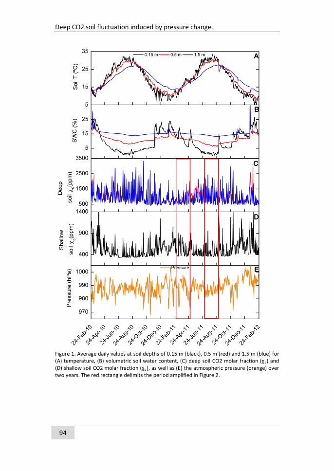
Deep CO2 soil fluctuation induced by pressure change.
94
Figure 1. Average daily values at soil depths of 0.15 m (black), 0.5 m (red) and 1.5 m (blue) for (A) temperature, (B) volumetric soil water content, (C) deep soil CO2 molar fraction (χc) and (D) shallow soil CO2 molar fraction (χc), as well as (E) the atmospheric pressure (orange) over two years. The red rectangle delimits the period amplified in Figure 2.
Results. Chapter 4
95
Soil CO2 molar fractions (χc) generally increase with depth, with a
constant baseline for each horizon over the years, but also with periodic
surges to more than double the mean value within a few days. The two deep
sensors behave similarly (Fig. 1C), with the blue line (1.5 m depth)
overlapping the red line (0.5 m depth) so nearly that the 0.5 m data are
practically obscured. They show clear annual patterns with maxima in
summer and minima in winter, similar means over the two years (χc ~1032
ppm at 0.5 m, and 994 ppm at 1.5 m) and rapid variability. By contrast, the
shallow sensor (Fig. 1D) has about half the mean (χc ~ 529 ppm CO2) and
notably less variability - in both frequency and magnitude. Also in contrast to
the deep case, shallow soil χc is highest in winter and lowest in summer.
Differences between the deep and shallow probes are less pronounced in
winter. Pressure (p) varies from 967-1007 hPa (Fig. 1E), with increased
variability in winter due to the passage of synoptic systems, and suppressed
variability in summer under the Mediterranean high. To clarify the relation
between χc and p, we focus on two different periods of 2011 (Fig. 1. Red
rectangles): the growing period from March to May and the dry period from
July to September.
Synoptic patterns
Table 1 shows the mean and standard error of environmental variables
associated with varying soil CO2 molar fractions (χc) during both periods. For
the growing period (from March to May) deep soil CO2 molar fractions (χc)
are nearly double (χc ~943 ppm at 0.5 m, and 813 ppm at 1.5 m) the shallow
χc (~515 ppm at 0.15 m). At all depths the soil temperature has a similar mean
(15.6 ºC, 15.7 ºC and 15.5 ºC at 0.15 m, 0.5 m and 1.5 m respectively) as can
be appreciated in Figure 1A, and the soil water content increases with depth
with values of 11.1 %, 11.6 %, and 15.3 %. During the dry period (from July
to September) the deep soil CO2 molar fractions (χc) are more than double (χc
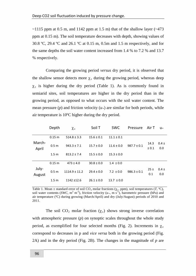
Deep CO2 soil fluctuation induced by pressure change.
96
~1115 ppm at 0.5 m, and 1142 ppm at 1.5 m) that of the shallow layer (~473
ppm at 0.15 m). The soil temperature decreases with depth, showing values of
30.8 ºC, 29.4 ºC and 26.1 ºC at 0.15 m, 0.5m and 1.5 m respectively, and for
the same depths the soil water content increased from 1.4 % to 7.2 % and 13.7
% respectively.
Comparing the growing period versus dry period, it is observed that
the shallow sensor detects more χc during the growing period, whereas deep
χc is higher during the dry period (Table 1). As is commonly found in
semiarid sites, soil temperatures are higher in the dry period than in the
growing period, as opposed to what occurs with the soil water content. The
mean pressure (p) and friction velocity (u*) are similar for both periods, while
air temperature is 10ºC higher during the dry period.
Depth χc Soil T SWC Pressure Air T u*
March-April
0.15 m 514.8 ± 3.3 15.6 ± 0.1 11.1 ± 0.1
987.7 ± 0.1 14.3 ± 0.1
0.4 ± 0.0
0.5 m 943.3 ± 7.1 15.7 ± 0.0 11.6 ± 0.0
1.5 m 813.2 ± 7.4 15.5 ± 0.0 15.3 ± 0.0
July-August
0.15 m 473 ± 4.0 30.8 ± 0.0 1.4 ± 0.0
986.3 ± 0.1 25 ± 0.1
0.4 ± 0.0
0.5 m 1114.9 ± 11.2 29.4 ± 0.0 7.2 ± 0.0
1.5 m 1142 ±12.6 26.1 ± 0.0 13.7 ± 0.0
Table 1. Mean ± standard error of soil CO2 molar fractions (χc, ppm), soil temperatures (T, ºC), soil water contents (SWC, m3 m-3), friction velocity (u*, m s-1), barometric pressure (hPa) and air temperature (ºC) during growing (March/April) and dry (July/August) periods of 2010 and 2011.
The soil CO2 molar fraction (χc) shows strong inverse correlation
with atmospheric pressure (p) on synoptic scales throughout the whole study
period, as exemplified for four selected months (Fig. 2). Increments in χc
correspond to decreases in p and vice versa both in the growing period (Fig.
2A) and in the dry period (Fig. 2B). The changes in the magnitude of p are
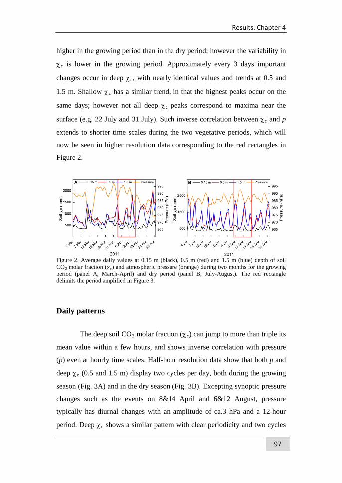
Results. Chapter 4
97
higher in the growing period than in the dry period; however the variability in
χc is lower in the growing period. Approximately every 3 days important
changes occur in deep χc, with nearly identical values and trends at 0.5 and
1.5 m. Shallow χc has a similar trend, in that the highest peaks occur on the
same days; however not all deep χc peaks correspond to maxima near the
surface (e.g. 22 July and 31 July). Such inverse correlation between χc and p
extends to shorter time scales during the two vegetative periods, which will
now be seen in higher resolution data corresponding to the red rectangles in
Figure 2.
Figure 2. Average daily values at 0.15 m (black), 0.5 m (red) and 1.5 m (blue) depth of soil CO2 molar fraction (χc) and atmospheric pressure (orange) during two months for the growing period (panel A, March-April) and dry period (panel B, July-August). The red rectangle delimits the period amplified in Figure 3.
Daily patterns
The deep soil CO2 molar fraction (χc) can jump to more than triple its
mean value within a few hours, and shows inverse correlation with pressure
(p) even at hourly time scales. Half-hour resolution data show that both p and
deep χc (0.5 and 1.5 m) display two cycles per day, both during the growing
season (Fig. 3A) and in the dry season (Fig. 3B). Excepting synoptic pressure
changes such as the events on 8&14 April and 6&12 August, pressure
typically has diurnal changes with an amplitude of ca.3 hPa and a 12-hour
period. Deep χc shows a similar pattern with clear periodicity and two cycles
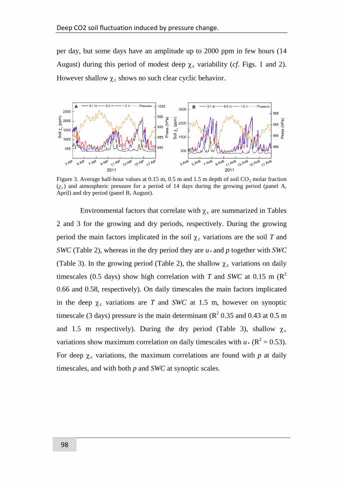
Deep CO2 soil fluctuation induced by pressure change.
98
per day, but some days have an amplitude up to 2000 ppm in few hours (14
August) during this period of modest deep χc variability (cf. Figs. 1 and 2).
However shallow χc shows no such clear cyclic behavior.
Figure 3. Average half-hour values at 0.15 m, 0.5 m and 1.5 m depth of soil CO2 molar fraction (χc) and atmospheric pressure for a period of 14 days during the growing period (panel A, April) and dry period (panel B, August).
Environmental factors that correlate with χc are summarized in Tables
2 and 3 for the growing and dry periods, respectively. During the growing
period the main factors implicated in the soil χc variations are the soil T and
SWC (Table 2), whereas in the dry period they are u* and p together with SWC
(Table 3). In the growing period (Table 2), the shallow χc variations on daily
timescales (0.5 days) show high correlation with T and SWC at 0.15 m (R2
0.66 and 0.58, respectively). On daily timescales the main factors implicated
in the deep χc variations are T and SWC at 1.5 m, however on synoptic
timescale (3 days) pressure is the main determinant (R2 0.35 and 0.43 at 0.5 m
and 1.5 m respectively). During the dry period (Table 3), shallow χc
variations show maximum correlation on daily timescales with u* (R2 = 0.53).
For deep χc variations, the maximum correlations are found with p at daily
timescales, and with both p and SWC at synoptic scales.
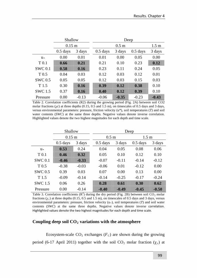
Results. Chapter 4
99
Shallow Deep
0.15 m 0.5 m 1.5 m
0.5 days 3 days 0.5 days 3 days 0.5 days 3 days
u* 0.00 0.01 0.01 0.00 0.05 0.00 T 0.1 0.66 0.21 0.21 0.10 0.23 0.12
SWC 0.1 0.58 0.16 0.23 0.11 0.24 0.05 T 0.5 0.04 0.03 0.12 0.03 0.12 0.01
SWC 0.5 0.05 0.05 0.12 0.03 0.15 0.03 T 1.5 0.30 0.16 0.39 0.12 0.38 0.10
SWC 1.5 0.37 0.16 0.40 0.12 0.39 0.10 Pressure 0.00 -0.13 -0.06 -0.35 -0.23 -0.43
Table 2. Correlation coefficients (R2) during the growing period (Fig. 2A) between soil CO2 molar fractions (χc) at three depths (0.15, 0.5 and 1.5 m), on timescales of 0.5 days and 3 days, versus environmental parameters: pressure, friction velocity (u*), soil temperatures (T) and soil water contents (SWC) at the same three depths. Negative values denote inverse correlation. Highlighted values denote the two highest magnitudes for each depth and time scale.
Shallow Deep
0.15 m 0.5 m 1.5 m
0.5 days 3 days 0.5 days 3 days 0.5 days 3 days
u* 0.53 0.24 0.04 0.05 0.08 0.06 T 0.1 0.46 0.32 0.05 0.10 0.12 0.10
SWC 0.1 -0.46 -0.33 -0.07 -0.11 -0.14 -0.12 T 0.5 -0.38 -0.03 -0.06 0.01 -0.12 0.00
SWC 0.5 0.39 0.03 0.07 0.00 0.13 0.00 T 1.5 -0.09 -0.14 -0.14 -0.25 -0.17 -0.24
SWC 1.5 0.06 0.26 0.28 0.61 0.30 0.62 Pressure 0.00 -0.14 -0.40 -0.49 -0.45 -0.50
Table 3. Correlation coefficients (R2) during the dry period (Fig. 2B) between soil CO2 molar fractions (χc) at three depths (0.15, 0.5 and 1.5 m), on timescales of 0.5 days and 3 days, versus environmental parameters: pressure, friction velocity (u*), soil temperatures (T) and soil water contents (SWC) at the same three depths. Negative values denote inverse correlation. Highlighted values denote the two highest magnitudes for each depth and time scale.
Coupling deep soil CO2 variations with the atmosphere
Ecosystem-scale CO2 exchanges (FC) are shown during the growing
period (6-17 April 2011) together with the soil CO2 molar fraction (χc) at
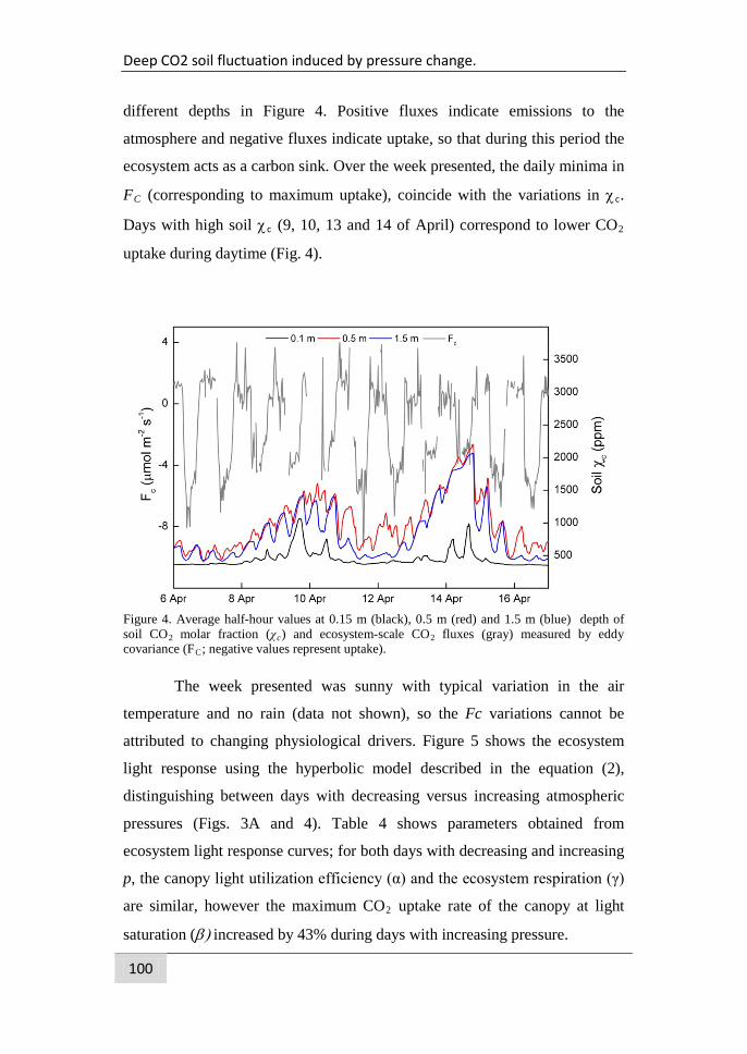
Deep CO2 soil fluctuation induced by pressure change.
100
different depths in Figure 4. Positive fluxes indicate emissions to the
atmosphere and negative fluxes indicate uptake, so that during this period the
ecosystem acts as a carbon sink. Over the week presented, the daily minima in
FC (corresponding to maximum uptake), coincide with the variations in χc.
Days with high soil χc (9, 10, 13 and 14 of April) correspond to lower CO2
uptake during daytime (Fig. 4).
Figure 4. Average half-hour values at 0.15 m (black), 0.5 m (red) and 1.5 m (blue) depth of soil CO2 molar fraction (χc) and ecosystem-scale CO2 fluxes (gray) measured by eddy covariance (FC; negative values represent uptake).
The week presented was sunny with typical variation in the air
temperature and no rain (data not shown), so the Fc variations cannot be
attributed to changing physiological drivers. Figure 5 shows the ecosystem
light response using the hyperbolic model described in the equation (2),
distinguishing between days with decreasing versus increasing atmospheric
pressures (Figs. 3A and 4). Table 4 shows parameters obtained from
ecosystem light response curves; for both days with decreasing and increasing
p, the canopy light utilization efficiency (α) and the ecosystem respiration (γ)
are similar, however the maximum CO2 uptake rate of the canopy at light
saturation (β) increased by 43% during days with increasing pressure.
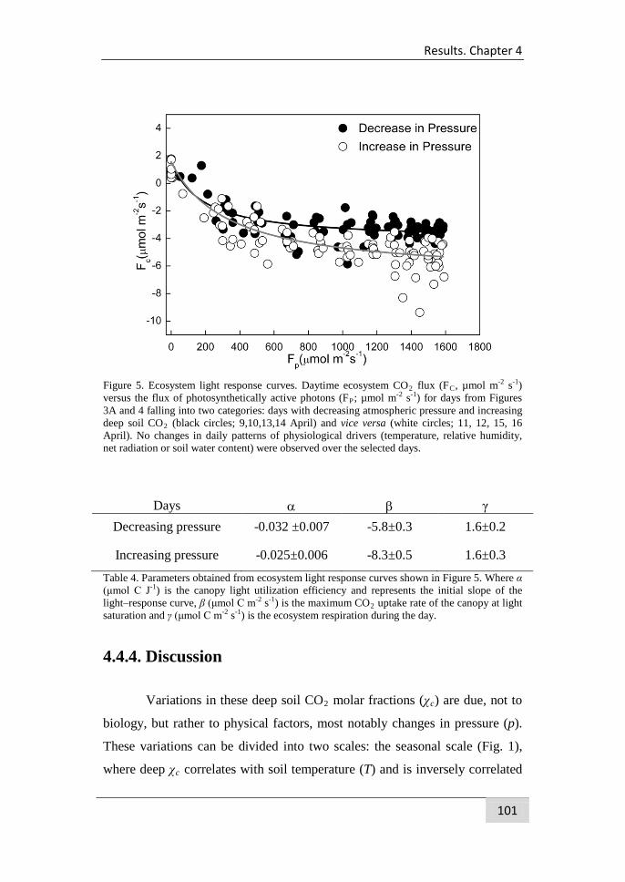
Results. Chapter 4
101
Figure 5. Ecosystem light response curves. Daytime ecosystem CO2 flux (FC, µmol m-2 s-1) versus the flux of photosynthetically active photons (FP; µmol m-2 s-1) for days from Figures 3A and 4 falling into two categories: days with decreasing atmospheric pressure and increasing deep soil CO2 (black circles; 9,10,13,14 April) and vice versa (white circles; 11, 12, 15, 16 April). No changes in daily patterns of physiological drivers (temperature, relative humidity, net radiation or soil water content) were observed over the selected days.
Days α β γ Decreasing pressure -0.032 ±0.007 -5.8±0.3 1.6±0.2
Increasing pressure -0.025±0.006 -8.3±0.5 1.6±0.3
Table 4. Parameters obtained from ecosystem light response curves shown in Figure 5. Where α (μmol C J-1) is the canopy light utilization efficiency and represents the initial slope of the light–response curve, β (μmol C m-2 s-1) is the maximum CO2 uptake rate of the canopy at light saturation and γ (μmol C m-2 s-1) is the ecosystem respiration during the day.
4.4.4. Discussion
Variations in these deep soil CO2 molar fractions (χc) are due, not to
biology, but rather to physical factors, most notably changes in pressure (p).
These variations can be divided into two scales: the seasonal scale (Fig. 1),
where deep χc correlates with soil temperature (T) and is inversely correlated
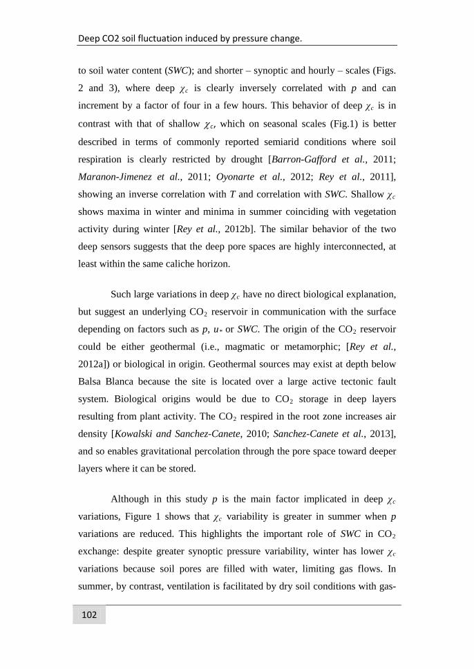
Deep CO2 soil fluctuation induced by pressure change.
102
to soil water content (SWC); and shorter – synoptic and hourly – scales (Figs.
2 and 3), where deep χc is clearly inversely correlated with p and can
increment by a factor of four in a few hours. This behavior of deep χc is in
contrast with that of shallow χc, which on seasonal scales (Fig.1) is better
described in terms of commonly reported semiarid conditions where soil
respiration is clearly restricted by drought [Barron-Gafford et al., 2011;
Maranon-Jimenez et al., 2011; Oyonarte et al., 2012; Rey et al., 2011],
showing an inverse correlation with T and correlation with SWC. Shallow χc
shows maxima in winter and minima in summer coinciding with vegetation
activity during winter [Rey et al., 2012b]. The similar behavior of the two
deep sensors suggests that the deep pore spaces are highly interconnected, at
least within the same caliche horizon.
Such large variations in deep χc have no direct biological explanation,
but suggest an underlying CO2 reservoir in communication with the surface
depending on factors such as p, u* or SWC. The origin of the CO2 reservoir
could be either geothermal (i.e., magmatic or metamorphic; [Rey et al.,
2012a]) or biological in origin. Geothermal sources may exist at depth below
Balsa Blanca because the site is located over a large active tectonic fault
system. Biological origins would be due to CO2 storage in deep layers
resulting from plant activity. The CO2 respired in the root zone increases air
density [Kowalski and Sanchez-Canete, 2010; Sanchez-Canete et al., 2013],
and so enables gravitational percolation through the pore space toward deeper
layers where it can be stored.
Although in this study p is the main factor implicated in deep χc
variations, Figure 1 shows that χc variability is greater in summer when p
variations are reduced. This highlights the important role of SWC in CO2
exchange: despite greater synoptic pressure variability, winter has lower χc
variations because soil pores are filled with water, limiting gas flows. In
summer, by contrast, ventilation is facilitated by dry soil conditions with gas-
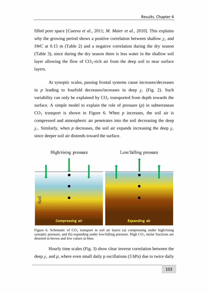
Results. Chapter 4
103
filled pore space [Cuezva et al., 2011; M. Maier et al., 2010]. This explains
why the growing period shows a positive correlation between shallow χc and
SWC at 0.15 m (Table 2) and a negative correlation during the dry season
(Table 3), since during the dry season there is less water in the shallow soil
layer allowing the flow of CO2-rich air from the deep soil to near surface
layers.
At synoptic scales, passing frontal systems cause increases/decreases
in p leading to fourfold decreases/increases in deep χc (Fig. 2). Such
variability can only be explained by CO2 transported from depth towards the
surface. A simple model to explain the role of pressure (p) in subterranean
CO2 transport is shown in Figure 6. When p increases, the soil air is
compressed and atmospheric air penetrates into the soil decreasing the deep
χc. Similarly, when p decreases, the soil air expands increasing the deep χc
since deeper soil air distends toward the surface.
Figure 6. Schematic of CO2 transport in soil air layers (a) compressing under high/rising synoptic pressure, and (b) expanding under low/falling pressure. High CO2 molar fractions are denoted in brown and low values in blue.
Hourly time scales (Fig. 3) show clear inverse correlation between the
deep χc and p, where even small daily p oscillations (3 hPa) due to twice daily
Deep CO2 soil fluctuation induced by pressure change.
104
atmospheric tides (Lindzen, 1979) generate large variations in χc at depth
(2000 ppm; e.g., falling χc on 12 August, Fig. 3B). Deep soil χc (0.5 and 1.5
m) shows two cycles per day, in rhythm with p, whereas shallow χc has just
one. This is consistent with correlations with the friction velocity and
biological drivers (T, SWC), but not with p (Table 3). Shallow χc is more
affected by friction velocity because it is in the upper part of the soil, and thus
more easily ventilated decreasing χc [Hirsch et al., 2004; Sanchez-Canete et
al., 2011]. Similarly, Rey et al. (2012a) concluded that the wind was the main
driver of the net ecosystem carbon balance at this experimental site.
The effects of emissions from deep CO2 soil were registered in the
atmosphere driven by synoptic pressure changes. The light-response curves
demonstrated that on both consecutive and non-consecutive days and near-
constant environmental conditions (temperature, relative humidity, net
radiation and soil water content), the maximum downward CO2 flux toward
the canopy at light saturation increased by 43% during days with increasing
synoptic pressure, versus those with falling pressure. This is in accordance
with the explanatory diagram of Figure 6. With rising pressure, part of the
CO2 respired by plants tends to accumulate in the soil, registering more
negative eddy fluxes and therefore obtaining a high value of β, which might
be interpreted erroneously as the maximum CO2 uptake rate of the canopy at
light saturation (as in Eq. 2). However, with falling pressure, both CO2 stored
in the soil and that respired by plants is emitted to the atmosphere, making
eddy fluxes less negative and lowering the value of β. The results presented in
this paper invite research on other semiarid ecosystems regarding the
influence of synoptic pressure changes on variations in deep soil CO2 molar
fractions and its role on the net ecosystem carbon balance.
Results. Chapter 4
105
4.4.5. Conclusions
This study reveals that during both growing periods and dry periods,
variations in the deep soil CO2 molar fraction (χc) are due predominantly to
atmospheric pressure (p) variations and not directly to biological influences.
In a few hours, the deep χc can increase or decrease fourfold, highlighting the
need for continuous (versus sporadic) monitoring of soil CO2 effluxes. Deep
χc has a pattern with two cycles per day, due to p oscillations caused by
atmospheric tides. Nonetheless shallow χc has a pattern with one cycle per
day, due to it is dependence mainly on the friction velocity during the dry
period and on biological factors during both dry and growing periods,
showing maxima for this semi-arid ecosystem when soil water content is not
limiting, with temperature dependence as well. The effects of emissions from
deep soil CO2 were registered in the atmosphere driven by synoptic pressure
changes: on days with rising pressure the downward CO2 flux is higher than
days with falling pressure because on these days CO2 respired by plants
accumulates in the soil. Future studies focused on determining the net
ecosystem carbon balance should not rely exclusively on Fick's law to
calculate soil CO2 effluxes from profile data.
Acknowledgements
This research was funded by the Andalusian regional government
project GEOCARBO (P08-RNM-3721) and GLOCHARID, including
European Union ERDF funds, with support from Spanish Ministry of Science
and Innovation projects Carbored-II (CGL2010-22193-C04-02), SOILPROF
(CGL2011-15276-E) and CARBORAD (CGL2011-27493), as well as the
European Community's Seventh Framework Programme (FP7/2007-2013)
under grant agreement n° 244122. We wish to thank Cecilio Oyonarte for
useful comments on the manuscript.
Deep CO2 soil fluctuation induced by pressure change.
106
References
Barron-Gafford, G. A., R. L. Scott, G. D. Jenerette, and T. E. Huxman (2011),
The relative controls of temperature, soil moisture, and plant
functional group on soil CO2 efflux at diel, seasonal, and annual
scales, J. Geophys. Res.-Biogeosci., 116, G01023.
Bowling, D. R., and W. J. Massman (2011), Persistent wind-induced
enhancement of diffusive CO2 transport in a mountain forest
snowpack, J. Geophys. Res.-Biogeosci., 116, G04006.
Chapin, F. S., et al. (2006), Reconciling carbon-cycle concepts, terminology,
and methods, Ecosystems, 9(7), 1041-1050.
Comas, X., L. Slater, and A. Reeve (2005), Spatial variability in biogenic gas
accumulations in peat soils is revealed by ground penetrating radar
(GPR), Geophys. Res. Lett., 32(8), L08401.
Comas, X., L. Slater, and A. Reeve (2007), In situ monitoring of free-phase
gas accumulation and release in peatlands using ground penetrating
radar (GPR), Geophys. Res. Lett., 34(6), L06402.
Comas, X., L. Slater, and A. S. Reeve (2011), Atmospheric pressure drives
changes in the vertical distribution of biogenic free-phase gas in a
northern peatland, J. Geophys. Res.-Biogeosci., 116, G04014.
Cuezva, S., A. Fernandez-Cortes, D. Benavente, P. Serrano-Ortiz, A. S.
Kowalski, and S. Sanchez-Moral (2011), Short-term CO2(g) exchange
between a shallow karstic cavity and the external atmosphere during
summer: Role of the surface soil layer, Atmospheric Environment,
45(7), 1418-1427.
Emmerich, E. W. (2003), Carbon dioxide fluxes in a semiarid environment
with high carbonate soils, Agric. For. Meteorol., 116, 91-102.
Falge, E., et al. (2002), Seasonality of ecosystem respiration and gross
primary production as derived from FLUXNET measurements, Agric.
For. Meteorol., 113(1-4), 53-74.
Results. Chapter 4
107
Falge, E., et al. (2001), Gap filling strategies for defensible annual sums of net
ecosystem exchange, Agric. For. Meteorol., 107(1), 43-69.
Fujiyoshi, R., Y. Haraki, T. Sumiyoshi, H. Amano, I. Kobal, and J. Vaupotic
(2010), Tracing the sources of gaseous components (Rn-222, CO2 and
its carbon isotopes) in soil air under a cool-deciduous stand in
Sapporo, Japan, Environmental Geochemistry and Health, 32(1), 73-
82.
Granieri, D., G. Chiodini, W. Marzocchi, and R. Avino (2003), Continuous
monitoring of CO2 soil diffuse degassing at Phlegraean Fields (Italy):
influence of environmental and volcanic parameters, Earth Planet.
Sci. Lett., 212(1-2), 167-179.
Hirsch, A. I., S. E. Trumbore, and M. L. Goulden (2004), The surface CO2
gradient and pore-space storage flux in a high-porosity litter layer,
Tellus Ser. B-Chem. Phys. Meteorol., 56(4), 312-321.
Huwald, H., J. S. Selker, S. W. Tyler, M. Calaf, N. C. van de Giesen, and M.
B. Parlange (2012), Carbon monoxide as a tracer of gas transport in
snow and other natural porous media, Geophys. Res. Lett., 39,
L02504.
Kowalski, A. S., and E. P. Sanchez-Canete (2010), A New Definition of the
Virtual Temperature, Valid for the Atmosphere and the CO2-Rich Air
of the Vadose Zone, Journal of Applied Meteorology and
Climatology, 49(8), 1692-1695.
Kowalski, A. S., P. M. Anthoni, R. J. Vong, A. C. Delany, and G. D. Maclean
(1997), Deployment and evaluation of a system for ground-based
measurement of cloud liquid water turbulent fluxes, Journal of
Atmospheric and Oceanic Technology, 14(3), 468-479.
Kowalski, A. S., P. Serrano-Ortiz, I. A. Janssens, S. Sanchez-Moraic, S.
Cuezva, F. Domingo, A. Were, and L. Alados-Arboledas (2008), Can
flux tower research neglect geochemical CO2 exchange?, Agric. For.
Meteorol., 148(6-7), 1045-1054.
Deep CO2 soil fluctuation induced by pressure change.
108
Lewicki, J. L., M. L. Fischer, and G. E. Hilley (2008), Six-week time series of
eddy covariance CO2 flux at Mammoth Mountain, California:
Performance evaluation and role of meteorological forcing, J.
Volcanol. Geotherm. Res., 171(3-4), 178-190.
Lewicki, J. L., G. E. Hilley, T. Tosha, R. Aoyagi, K. Yamamoto, and S. M.
Benson (2007), Dynamic coupling of volcanic CO2 flow and wind at
the Horseshoe Lake tree kill, Mammoth Mountain, California,
Geophys. Res. Lett., 34(3), L03401.
Maier, M., H. Schack-Kirchner, E. E. Hildebrand, and J. Holst (2010), Pore-
space CO2 dynamics in a deep, well-aerated soil, European Journal of
Soil Science, 61(6), 877-887.
Maier, M., H. Schack-Kirchner, M. Aubinet, S. Goffi, B. Longdoz, and F.
Parent (2012), Turbulence Effect on Gas Transport in Three
Contrasting Forest Soils, Soil Sci. Soc. Am. J., 76(5), 1518-1528.
Maranon-Jimenez, S., J. Castro, A. S. Kowalski, P. Serrano-Ortiz, B. R.
Reverter, E. P. Sanchez-Canete, and R. Zamora (2011), Post-fire soil
respiration in relation to burnt wood management in a Mediterranean
mountain ecosystem, Forest Ecology and Management, 261(8), 1436-
1447.
Massman, W. J., R. A. Sommerfeld, A. R. Mosier, K. F. Zeller, T. J. Hehn,
and S. G. Rochelle (1997), A model investigation of turbulence-
driven pressure-pumping effects on the rate of diffusion of CO2,
N2O, and CH4 through layered snowpacks, J. Geophys. Res.-Atmos.,
102(D15), 18851-18863.
Mielnick, P., W. A. Dugas, K. Mitchell, and K. Havstad (2005), Long-term
measurements of CO2 flux and evapotranspiration in a Chihuahuan
desert grassland, J. Arid. Environ., 60(3), 423-436.
Nachshon, U., M. Dragila, and N. Weisbrod (2012), From atmospheric winds
to fracture ventilation: Cause and effect, J. Geophys. Res.-Biogeosci.,
117.
Results. Chapter 4
109
Oyonarte, C., A. Rey, J. Raimundo, I. Miralles, and P. Escribano (2012), The
use of soil respiration as an ecological indicator in arid ecosystems of
the SE of Spain: Spatial variability and controlling factors, Ecol.
Indic., 14(1), 40-49.
Plestenjak, G., K. Eler, D. Vodnik, M. Ferlan, M. Cater, T. Kanduc, P.
Simoncic, and N. Ogrinc (2012), Sources of soil CO2 in calcareous
grassland with woody plant encroachment, Journal of Soils and
Sediments, 12(9), 1327-1338.
Reicosky, D. C., R. W. Gesch, S. W. Wagner, R. A. Gilbert, C. D. Wente, and
D. R. Morris (2008), Tillage and wind effects on soil CO2
concentrations in muck soils, Soil & Tillage Research, 99(2), 221-
231.
Rey, A., G. Etiope, L. Belelli-Marchesini, D. Papale, and R. Valentini
(2012a), Geologic carbon sources may confound ecosystem carbon
balance estimates: Evidence from a semiarid steppe in the southeast of
Spain, J. Geophys. Res.-Biogeosci., 117, G03034.
Rey, A., E. Pegoraro, C. Oyonarte, A. Were, P. Escribano, and J. Raimundo
(2011), Impact of land degradation on soil respiration in a steppe
(Stipa tenacissima L.) semi-arid ecosystem in the SE of Spain, Soil
Biol. Biochem., 43(2), 393-403.
Rey, A., L. Belelli-Marchesini, A. Were, P. Serrano-Ortiz, G. Etiope, D.
Papale, F. Domingo, and E. Pegoraro (2012b), Wind as a main driver
of the net ecosystem carbon balance of a semiarid Mediterranean
steppe in the South East of Spain, Glob. Change Biol., 18(2), 539-
554.
Rogie, J. D., D. M. Kerrick, M. L. Sorey, G. Chiodini, and D. L. Galloway
(2001), Dynamics of carbon dioxide emission at Mammoth Mountain,
California, Earth Planet. Sci. Lett., 188(3-4), 535-541.
Sanchez-Canete, E. P., P. Serrano-Ortiz, F. Domingo, and A. S. Kowalski
(2013), Cave ventilation is influenced by variations in the CO2-
dependent virtual temperature, Int. J. Speleol., 42, 1-8.
Deep CO2 soil fluctuation induced by pressure change.
110
Sanchez-Canete, E. P., P. Serrano-Ortiz, A. S. Kowalski, C. Oyonarte, and F.
Domingo (2011), Subterranean CO2 ventilation and its role in the net
ecosystem carbon balance of a karstic shrubland, Geophys. Res. Lett.,
38, L09802.
Seok, B., D. Helmig, M. W. Williams, D. Liptzin, K. Chowanski, and J.
Hueber (2009), An automated system for continuous measurements of
trace gas fluxes through snow: an evaluation of the gas diffusion
method at a subalpine forest site, Niwot Ridge, Colorado,
Biogeochemistry, 95(1), 95-113.
Serrano-Ortiz, P., M. Roland, S. Sanchez-Moral, I. A. Janssens, F. Domingo,
Y. Godderis, and A. S. Kowalski (2010), Hidden, abiotic CO2 flows
and gaseous reservoirs in the terrestrial carbon cycle: Review and
perspectives, Agric. For. Meteorol., 150(3), 321-329.
Serrano-Ortiz, P., F. Domingo, A. Cazorla, A. Were, S. Cuezva, L.
Villagarcia, L. Alados-Arboledas, and A. S. Kowalski (2009),
Interannual CO2 exchange of a sparse Mediterranean shrubland on a
carbonaceous substrate, J. Geophys. Res.-Biogeosci., 114, G04015.
Stull, R. B. (1988), An introduction to Boundary Layer Meteorology, 667 pp.,
Kluwer Academic Publishers, Dordrecht, The Netherlands.
Subke, J. A., M. Reichstein, and J. D. Tenhunen (2003), Explaining temporal
variation in soil CO2 efflux in a mature spruce forest in Southern
Germany, Soil Biol. Biochem., 35(11), 1467-1483.
Takle, E. S., W. J. Massman, J. R. Brandle, R. A. Schmidt, X. H. Zhou, I. V.
Litvina, R. Garcia, G. Doyle, and C. W. Rice (2004), Influence of
high-frequency ambient pressure pumping on carbon dioxide efflux
from soil, Agric. For. Meteorol., 124(3-4), 193-206.
Webb, E. K., G. I. Pearman, and R. Leuning (1980), Correction of flux
measurements for density effects due to heat and water vapor transfer,
Q. J. R. Meteorol. Soc., 106(447), 85-100.
Were, A., P. Serrano-Ortiz, C. M. de Jong, L. Villagarcia, F. Domingo, and A.
S. Kowalski (2010), Ventilation of subterranean CO2 and Eddy

Results. Chapter 4
111
covariance incongruities over carbonate ecosystems, Biogeosciences,
7(3), 859-867.
Wilks, D. S. (2006), Statistical Methods in the Atmospheric Sciences, 2 ed.,
649 pp., Academic Press.

Deep CO2 soil fluctuation induced by pressure change.
112
General discussion and conclusions
113
5. General discussion and conclusions
5.1 General discussion
State of the art Subterranean CO2
The study of CO2 underground in both soils and caves has been
undertaken since the late 20th century [Crowther, 1983; Ek and Gewelt, 1985;
Kiefer and Amey, 1992]. Such studies have focused mainly on measurements
in the first few centimeters of soil, through air sampling and subsequent
laboratory analysis. From the last decade of 20th century until the present,
underground CO2 studies have mainly focused on surface-atmosphere CO2
exchanges, through the use of surface chambers and disregarding what
happens at depth.
In the first decade of the 21st century new studies have arisen focused
on measurements of subterranean CO2. Hirsch et al. [2002] is one of the first
authors that monitored CO2 behavior with an automated soil gas sampling
system in a vertical profile (0-50cm), followed by others scientists [DeSutter
et al., 2006; Hirsch et al., 2004; Jassal et al., 2005; Novak, 2007; Pumpanen
et al., 2008; Risk et al., 2008; Takahashi et al., 2004; Tang et al., 2003].
Many of these authors estimated CO2 fluxes emitted by applying Fick’s Law,
also termed the gradient method. However, our studies show that Fick's law is
not applicable in semi-arid lands when the wind is high [Sanchez-Canete et
al., 2011] or when pressure changes [Sanchez-Canete et al., 2013b].
In addition, studies of CO2 in caves have focused mainly on
identifying the factors involved in cave ventilation. Until the publication of
the article by Kowalski & Sánchez-Cañete, [2010] and subsequently Sánchez-
Cañete et al. [2013a], cave ventilation was determined as a function of
differences between outside and inside temperatures. However these articles
CO2 exchanges in deep soils and caves and their role in the NEBC
114
represent a landmark because they show the importance of CO2 in
determining the cave ventilation.
Now it is necessary to change the point of view regarding CO2
exchange studies from an inappropriately conceived static system in which all
CO2 respired is directly emitted by molecular processes to the atmosphere, to
a dynamic system with gas transport by three different processes: convection,
advection and molecular diffusion. It has been observed than soils can
exchange/store large CO2 amounts as a function of numerous natural
processes. Large amounts of CO2 are stored in the soil with possibility to be
exchanged with the atmosphere [Benavente et al., 2010; Ek and Gewelt, 1985]
through processes of convection, advection or molecular diffusion.
Convective processes are mainly relevant in caves, where the values of
relative humidity, temperature and CO2 molar fraction determine the
buoyancy of the external-internal air masses, and therefore determine when
ventilation can occur [Kowalski and Sanchez-Canete, 2010; Sanchez-Canete
et al., 2013a]. These convective processes also are important in large fractures
when temperature differences between surface and depth can generate air
convection, transporting CO2 from deep layers to the atmosphere. Advective
processes occur both in caves and in soils and the CO2 exchanges are mainly
due to three factors:
1) the wind, which can penetrate into the soil permitting forcing gas
exchange [Bowling and Massman, 2011; Maier et al., 2012; Sanchez-
Canete et al., 2011];
2) changes in atmospheric pressure, which compress and expand the soil
air allowing its exchange [Comas et al., 2011; Sanchez-Canete et al.,
2013b], and
3) changes in the water table; variations in the aquifer volumes can
provoke emission or storage of CO2 within the soil pore space as
demonstrated with variations due to ocean tides [Jiao and Li, 2004;
Werner et al., 2013].
General discussion and conclusions
115
Processes due to molecular diffusion are being widely applied in the
determination of soil-atmosphere gas exchanges [Barron-Gafford et al., 2011;
Bowling et al., 2011; Davidson and Trumbore, 1995; Pingintha et al., 2010;
Pumpanen et al., 2008]. However Fick’s Law should only be applied in the
absence of advective or convective processes.
Recent relevant publications
During the years of writing this dissertation, and since publication of
the first articles, numerous papers have emerged to improve knowledge of
CO2 exchanges between the atmosphere and the subsurface (caves and soils).
Articles focused on Cave-Atmosphere exchanges have focused mainly on
determining ventilation as a function of temperature differences, disregarding
the effects of air composition on buoyancy. Following publication of the
specious Badino [2009] article entitled "The legend of carbon dioxide
heaviness", and having reviewed literature that highlights high concentrations
of CO2 in soil air, Kowalski & Sánchez-Cañete in [2010] developed some
formulas to correctly determine the buoyancy of a CO2–rich air mass. Still,
some speleologists continued to use temperature differences to incorrectly
determine ventilation [e.g., Boch et al., 2011; J. Faimon and Licbinska, 2010;
J. Faimon et al., 2012; Gregoric et al., 2011; Kowalczk and Froelich, 2010].
This motivated the publication of Sanchez-Cañete et al. [2013a], who
provided a more practical overview, showing in different caves of the world
the substantial errors that can occur when the role of carbon dioxide is
ignored. Although some authors are already using the new equations to
correctly interpret ventilation in caves [Bourges et al., 2012; Jiří Faimon and
Lang, 2013; Fairchild and Baker, 2012; Nachshon et al., 2012], studies still
may be found that do not take into account the CO2 effect [Gregoric et al.,
2013].
CO2 exchanges in deep soils and caves and their role in the NEBC
116
Regarding the research line of soil-atmosphere CO2 exchanges,
numerous contributions to the literature have appeared over the past four
years. Deserving of special attention are publications determining CO2
exchange with the atmosphere through the use of subterranean profiles, using
the gradient method [Liang et al., 2010; Pingintha et al., 2010; Sullivan et al.,
2010]. Although in less in number, other studies have also appeared showing
that the gradient method, based on the Fick’s Law, is not always applicable
because the transport of gases from the ground to the atmosphere is affected
by other factors such the wind [Bowling and Massman, 2011; Nachshon et al.,
2012; Sanchez-Canete et al., 2011], soil thermal gradients [Ganot et al., 2012;
Moore et al., 2011; Weisbrod et al., 2009], or changes in pressure [Lampkin,
2010; Rinaldi et al., 2012; Sanchez-Canete et al., 2013b]. Despite these and
other publications, knowledge of subterranean CO2 dynamics is still a novel
research area in which there remain many gaps of understanding to enable
correct modeling [Perez-Priego et al., 2013; Roland et al., 2013].
Perspectives on future research
The study of subterranean CO2 is a field which can still be explored
from many points of view. I hope to continue along this same line of research
because it offers many opportunities for advancing the state of science. Here I
outline some lines of inquiry that could generate knowledge and clarify
uncertainties.
a) Additional subterranean CO2 profiles, such as those measured in the
Sierra de Gádor and in Balsa Blanca, could be installed in other
semiarid ecosystems around the world to check whether the results
from these sites can be extrapolated elsewhere. For this reason, in my
last research visit (2011) to the Southwest Watershed Research Center
General discussion and conclusions
117
(Arizona, EE UU), we installed several profiles whose data I intend to
analyze during the summer of 2013.
b) Monitor CO2 in different boreholes of the world, to characterize the
mean CO2 molar fraction in the different ecosystems, lithologies and
depths, and so estimate at the planetary scale: how much CO2 is
stored in the vadose zone? And furthermore, what factors are
implicated in its exchange with the atmosphere?
c) Monitor CO2 and heat fluxes between the atmosphere and boreholes,
fractures or caves. We have recently initiated such an effort at the
Nerja Cave (Málaga, Spain).
d) Investigate gas emissions produced - mainly in karst areas - due to
increments in the water table and consequent displacement of the air
to the atmosphere.
5.2 Conclusions
This thesis contributes to increase scientific knowledge on CO2
exchanges between the atmosphere and deep soil, distinguishing the drivers
involved in its transport. The main conclusions of the thesis are the following:
From a methodological point of view, never before has a study has
taken into account the role of underground CO2 in modifying air density,
despite numerous studies of the buoyancy of cave air. Due to results
developed in this thesis, it is now possible to determine when ventilation may
occur due to differences between the buoyancy of air masses. It has been
shown that in cases where CO2 molar fractions of internal air exceed
atmospheric values by an order of magnitude or more, it is necessary to take
into account the heaviness of CO2 when calculating the virtual temperature
and thereby buoyancy. If CO2 is not taken into account when external and
internal air masses have the same temperature, it can cause errors close to 9ºC
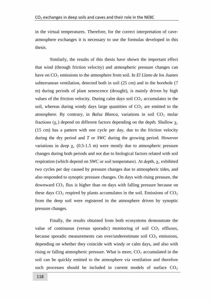
CO2 exchanges in deep soils and caves and their role in the NEBC
118
in the virtual temperatures. Therefore, for the correct interpretation of cave-
atmosphere exchanges it is necessary to use the formulas developed in this
thesis.
Similarly, the results of this thesis have shown the important effect
that wind (through friction velocity) and atmospheric pressure changes can
have on CO2 emissions to the atmosphere from soil. In El Llano de los Juanes
subterranean ventilation, detected both in soil (25 cm) and in the borehole (7
m) during periods of plant senescence (drought), is mainly driven by high
values of the friction velocity. During calm days soil CO2 accumulates in the
soil, whereas during windy days large quantities of CO2 are emitted to the
atmosphere. By contrary, in Balsa Blanca, variations in soil CO2 molar
fractions (χc) depend on different factors depending on the depth. Shallow χc
(15 cm) has a pattern with one cycle per day, due to the friction velocity
during the dry period and T or SWC during the growing period. However
variations in deep χc (0.5-1.5 m) were mostly due to atmospheric pressure
changes during both periods and not due to biological factors related with soil
respiration (which depend on SWC or soil temperature). At depth, χc exhibited
two cycles per day caused by pressure changes due to atmospheric tides, and
also responded to synoptic pressure changes. On days with rising pressure, the
downward CO2 flux is higher than on days with falling pressure because on
these days CO2 respired by plants accumulates in the soil. Emissions of CO2
from the deep soil were registered in the atmosphere driven by synoptic
pressure changes.
Finally, the results obtained from both ecosystems demonstrate the
value of continuous (versus sporadic) monitoring of soil CO2 effluxes,
because sporadic measurements can over/underestimate soil CO2 emissions,
depending on whether they coincide with windy or calm days, and also with
rising or falling atmospheric pressure. What is more, CO2 accumulated in the
soil can be quickly emitted to the atmosphere via ventilation and therefore
such processes should be included in current models of surface CO2
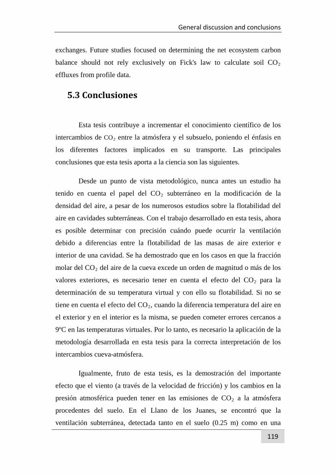
General discussion and conclusions
119
exchanges. Future studies focused on determining the net ecosystem carbon
balance should not rely exclusively on Fick's law to calculate soil CO2
effluxes from profile data.
5.3 Conclusiones
Esta tesis contribuye a incrementar el conocimiento científico de los
intercambios de CO2 entre la atmósfera y el subsuelo, poniendo el énfasis en
los diferentes factores implicados en su transporte. Las principales
conclusiones que esta tesis aporta a la ciencia son las siguientes.
Desde un punto de vista metodológico, nunca antes un estudio ha
tenido en cuenta el papel del CO2 subterráneo en la modificación de la
densidad del aire, a pesar de los numerosos estudios sobre la flotabilidad del
aire en cavidades subterráneas. Con el trabajo desarrollado en esta tesis, ahora
es posible determinar con precisión cuándo puede ocurrir la ventilación
debido a diferencias entre la flotabilidad de las masas de aire exterior e
interior de una cavidad. Se ha demostrado que en los casos en que la fracción
molar del CO2 del aire de la cueva excede un orden de magnitud o más de los
valores exteriores, es necesario tener en cuenta el efecto del CO2 para la
determinación de su temperatura virtual y con ello su flotabilidad. Si no se
tiene en cuenta el efecto del CO2, cuando la diferencia temperatura del aire en
el exterior y en el interior es la misma, se pueden cometer errores cercanos a
9ºC en las temperaturas virtuales. Por lo tanto, es necesario la aplicación de la
metodología desarrollada en esta tesis para la correcta interpretación de los
intercambios cueva-atmósfera.
Igualmente, fruto de esta tesis, es la demostración del importante
efecto que el viento (a través de la velocidad de fricción) y los cambios en la
presión atmosférica pueden tener en las emisiones de CO2 a la atmósfera
procedentes del suelo. En el Llano de los Juanes, se encontró que la
ventilación subterránea, detectada tanto en el suelo (0.25 m) como en una
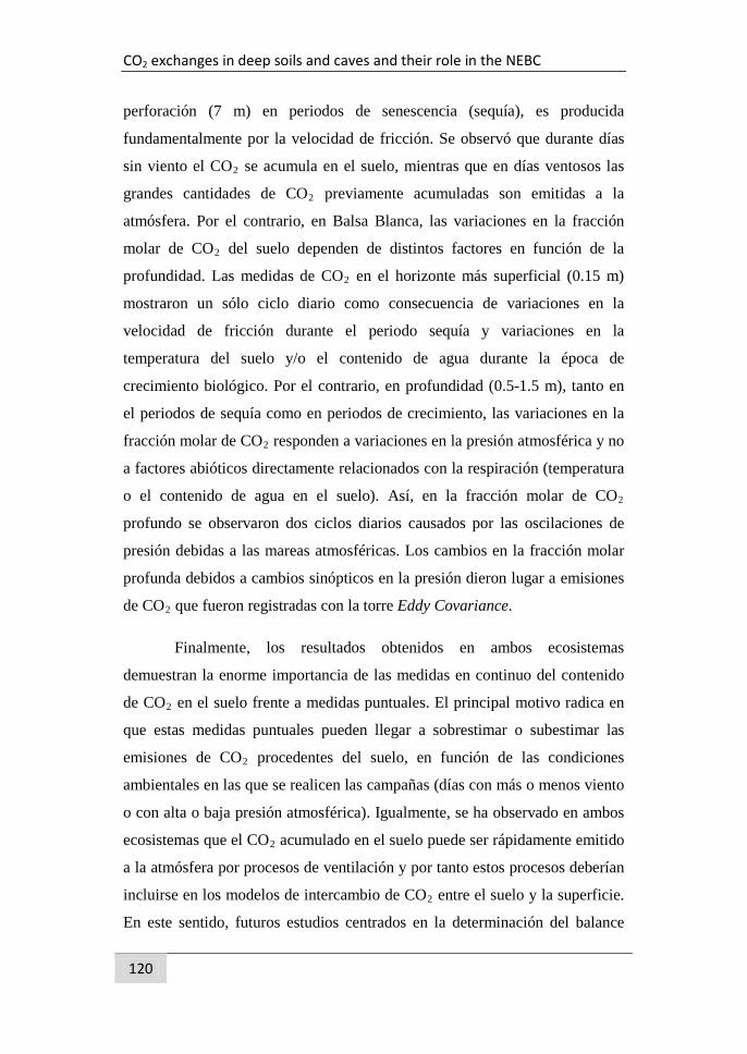
CO2 exchanges in deep soils and caves and their role in the NEBC
120
perforación (7 m) en periodos de senescencia (sequía), es producida
fundamentalmente por la velocidad de fricción. Se observó que durante días
sin viento el CO2 se acumula en el suelo, mientras que en días ventosos las
grandes cantidades de CO2 previamente acumuladas son emitidas a la
atmósfera. Por el contrario, en Balsa Blanca, las variaciones en la fracción
molar de CO2 del suelo dependen de distintos factores en función de la
profundidad. Las medidas de CO2 en el horizonte más superficial (0.15 m)
mostraron un sólo ciclo diario como consecuencia de variaciones en la
velocidad de fricción durante el periodo sequía y variaciones en la
temperatura del suelo y/o el contenido de agua durante la época de
crecimiento biológico. Por el contrario, en profundidad (0.5-1.5 m), tanto en
el periodos de sequía como en periodos de crecimiento, las variaciones en la
fracción molar de CO2 responden a variaciones en la presión atmosférica y no
a factores abióticos directamente relacionados con la respiración (temperatura
o el contenido de agua en el suelo). Así, en la fracción molar de CO2
profundo se observaron dos ciclos diarios causados por las oscilaciones de
presión debidas a las mareas atmosféricas. Los cambios en la fracción molar
profunda debidos a cambios sinópticos en la presión dieron lugar a emisiones
de CO2 que fueron registradas con la torre Eddy Covariance.
Finalmente, los resultados obtenidos en ambos ecosistemas
demuestran la enorme importancia de las medidas en continuo del contenido
de CO2 en el suelo frente a medidas puntuales. El principal motivo radica en
que estas medidas puntuales pueden llegar a sobrestimar o subestimar las
emisiones de CO2 procedentes del suelo, en función de las condiciones
ambientales en las que se realicen las campañas (días con más o menos viento
o con alta o baja presión atmosférica). Igualmente, se ha observado en ambos
ecosistemas que el CO2 acumulado en el suelo puede ser rápidamente emitido
a la atmósfera por procesos de ventilación y por tanto estos procesos deberían
incluirse en los modelos de intercambio de CO2 entre el suelo y la superficie.
En este sentido, futuros estudios centrados en la determinación del balance

General discussion and conclusions
121
neto de carbono no deberían basarse exclusivamente en la ley de Fick para
calcular las emisiones de CO2 procedentes de los datos de un perfil.
CO2 exchanges in deep soils and caves and their role in the NEBC
122
References
Badino, G. (2009), The legend of carbon dioxide heaviness, J. Cave Karst
Stud., 71(1), 100-107.
Barron-Gafford, G. A., R. L. Scott, G. D. Jenerette, and T. E. Huxman (2011),
The relative controls of temperature, soil moisture, and plant
functional group on soil CO2 efflux at diel, seasonal, and annual
scales, J. Geophys. Res.-Biogeosci., 116, G01023.
Benavente, J., I. Vadillo, F. Carrasco, A. Soler, C. Linan, and F. Moral
(2010), Air Carbon Dioxide Contents in the Vadose Zone of a
Mediterranean Karst, Vadose Zone J., 9(1), 126-136.
Boch, R., C. Spoetl, and S. Frisia (2011), Origin and palaeoenvironmental
significance of lamination in stalagmites from Katerloch Cave,
Austria, Sedimentology, 58(2), 508-531.
Bourges, F., P. Genthon, D. Genty, A. Mangin, and D. D'Hulst (2012),
Comment on "Carbon uptake by karsts in the Houzhai Basin,
southwest China" by Junhua Yan et al, J. Geophys. Res.-Biogeosci.,
117.
Bowling, D. R., and W. J. Massman (2011), Persistent wind-induced
enhancement of diffusive CO2 transport in a mountain forest
snowpack, J. Geophys. Res.-Biogeosci., 116, G04006.
Bowling, D. R., E. E. Grote, and J. Belnap (2011), Rain pulse response of soil
CO2 exchange by biological soil crusts and grasslands of the semiarid
Colorado Plateau, United States, J. Geophys. Res.-Biogeosci,
116(G3), G03028.
Comas, X., L. Slater, and A. S. Reeve (2011), Atmospheric pressure drives
changes in the vertical distribution of biogenic free-phase gas in a
northern peatland, J. Geophys. Res.-Biogeosci., 116, G04014.
Crowther, J. (1983), Carbon-dioxide concentrations in some tropical karst
soils, west Malaysia., Catena, 10(1-2), 27-39.
General discussion and conclusions
123
Davidson, E. A., and S. E. Trumbore (1995), Gas diffusivity and production
of CO2 in deep soils of the eastern amazon., Tellus Ser. B-Chem.
Phys. Meteorol., 47(5), 550-565.
DeSutter, T. M., T. J. Sauer, and T. B. Parkin (2006), Porous tubing for use in
monitoring soil CO2 concentrations, Soil Biol. Biochem., 38(9), 2676-
2681.
Ek, C., and M. Gewelt (1985), Carbon dioxide in cave atmospheres. New
results in Belgium and comparison with some other countries., Earth
Surf. Process. Landf., 10(2), 173-187.
Faimon, J., and M. Licbinska (2010), Carbon dioxide in the soils and adjacent
caves of the Moravian karst, Acta Carsologica, 39(3), 463-475.
Faimon, J., and M. Lang (2013), Variances in airflows during different
ventilation modes in a dynamic U-shaped cave, Int. J. Speleol., 42(2),
3.
Faimon, J., D. Troppova, V. Baldik, and R. Novotny (2012), Air circulation
and its impact on microclimatic variables in the Cisarska Cave
(Moravian Karst, Czech Republic), Int. J. Climatol., 32(4), 599-623.
Fairchild, I. J., and A. Baker (2012), Speleothem Science: from process to past
environments, Wiley-Blackwell.
Ganot, Y., M. I. Dragila, and N. Weisbrod (2012), Impact of thermal
convection on air circulation in a mammalian burrow under arid
conditions, J. Arid. Environ., 84, 51-62.
Gregoric, A., A. Zidansek, and J. Vaupotic (2011), Dependence of radon
levels in Postojna Cave on outside air temperature, Natural Hazards
and Earth System Sciences, 11(5), 1523-1528.
Gregoric, A., J. Vaupotic, and F. Gabrovsek (2013), Reasons for large
fluctuation of radon and CO2 levels in a dead-end passage of a karst
cave (Postojna Cave, Slovenia), NHESS, 13.
Hirsch, A. I., S. E. Trumbore, and M. L. Goulden (2002), Direct measurement
of the deep soil respiration accompanying seasonal thawing of a
boreal forest soil, J. Geophys. Res.-Atmos., 108(D3).
CO2 exchanges in deep soils and caves and their role in the NEBC
124
Hirsch, A. I., S. E. Trumbore, and M. L. Goulden (2004), The surface CO2
gradient and pore-space storage flux in a high-porosity litter layer,
Tellus Ser. B-Chem. Phys. Meteorol., 56(4), 312-321.
Jassal, R., A. Black, M. Novak, K. Morgenstern, Z. Nesic, and D. Gaumont-
Guay (2005), Relationship between soil CO2 concentrations and
forest-floor CO2 effluxes, Agric. For. Meteorol., 130(3-4), 176-192.
Jiao, J. J., and H. L. Li (2004), Breathing of coastal vadose zone induced by
sea level fluctuations, Geophys. Res. Lett., 31(11).
Kiefer, R. H., and R. G. Amey (1992), Concentrations and controls of soil
carbon-dioxide in sandy soil in the north-carolina coastal-plain,
Catena, 19(6), 539-559.
Kowalczk, A. J., and P. N. Froelich (2010), Cave air ventilation and CO2
outgassing by radon-222 modeling: How fast do caves breathe?, Earth
Planet. Sci. Lett., 289(1-2), 209-219.
Kowalski, A. S., and E. P. Sanchez-Canete (2010), A New Definition of the
Virtual Temperature, Valid for the Atmosphere and the CO2-Rich Air
of the Vadose Zone, Journal of Applied Meteorology and
Climatology, 49(8), 1692-1695.
Lampkin, D. J. (2010), Resolving barometric pressure waves in seasonal
snowpack with a prototype-embedded wireless sensor network,
Hydrological Processes, 24(14), 2014-2021.
Liang, N., T. Hirano, Z. M. Zheng, J. Tang, and Y. Fujinuma (2010), Soil
CO2 efflux of a larch forest in northern Japan, Biogeosciences, 7(11),
3447-3457.
Maier, M., H. Schack-Kirchner, M. Aubinet, S. Goffi, B. Longdoz, and F.
Parent (2012), Turbulence Effect on Gas Transport in Three
Contrasting Forest Soils, Soil Sci. Soc. Am. J., 76(5), 1518-1528.
Moore, J. R., V. Gischig, M. Katterbach, and S. Loew (2011), Air circulation
in deep fractures and the temperature field of an alpine rock slope,
Earth Surf. Process. Landf., 36(15), 1985-1996.
General discussion and conclusions
125
Nachshon, U., M. Dragila, and N. Weisbrod (2012), From atmospheric winds
to fracture ventilation: Cause and effect, J. Geophys. Res.-Biogeosci.,
117.
Novak, M. D. (2007), Determination of soil carbon dioxide source-density
profiles by inversion from soil-profile gas concentrations and surface
flux density for diffusion-dominated transport, Agric. For. Meteorol.,
146(3-4), 189-204.
Pingintha, N., M. Y. Leclerc, J. P. Beasley, G. S. Zhang, and C. Senthong
(2010), Assessment of the soil CO2 gradient method for soil CO2
efflux measurements: comparison of six models in the calculation of
the relative gas diffusion coefficient, 62, 1(47-58).
Perez-Priego, O., P. Serrano-Ortiz, E. P. Sanchez-Canete, F. Doming, and A.
S. Kowalski (2013), Isolating the effect of subterranean ventilation on
CO2 emissions from drylands to the atmosphere, Agric. For.
Meteorol. In review.
Pumpanen, J., H. Ilvesniemi, L. Kulmala, E. Siivola, H. Laakso, P. Kolari, C.
Helenelund, M. Laakso, M. Uusimaa, and P. Hari (2008), Respiration
in boreal forest soil as determined from carbon dioxide concentration
profile, Soil Sci. Soc. Am. J., 72(5), 1187-1196.
Rinaldi, A. P., J. Vandemeulebrouck, M. Todesco, and F. Viveiros (2012),
Effects of atmospheric conditions on surface diffuse degassing,
Journal of Geophysical Research-Solid Earth, 117.
Risk, D., L. Kellman, and H. Beltrami (2008), A new method for in situ soil
gas diffusivity measurement and applications in the monitoring of
subsurface CO2 production, J. Geophys. Res.-Biogeosci., 113(G2).
Roland, M., Serrano-Ortiz, P., Kowalski, A.S., Godderis, Y., Sanchez-Canete,
E.P., Ciais, P., Doming, F., Cuezva, S., Sanchez-Moral, S., Longdoz,
B., Yakir, D., Van Grieken, R., Schott, C., Cardell, C., Janssens, I.A.,
(2013). Atmospheric turbulence triggers pronounced diel pattern in
karst carbonate geochemistry. Biogeosciences Discuss. 10, 1207–
1227.
CO2 exchanges in deep soils and caves and their role in the NEBC
126
Sanchez-Canete, E. P., P. Serrano-Ortiz, F. Domingo, and A. S. Kowalski
(2013a), Cave ventilation is influenced by variations in the CO2-
dependent virtual temperature, Int. J. Speleol., 42, 1-8.
Sanchez-Canete, E. P., P. Serrano-Ortiz, A. S. Kowalski, C. Oyonarte, and F.
Domingo (2011), Subterranean CO2 ventilation and its role in the net
ecosystem carbon balance of a karstic shrubland, Geophys. Res. Lett.,
38, L09802.
Sanchez-Canete, E. P., A. S. Kowalski, P. Serrano-Ortiz, P.-P. O., and F.
Domingo (2013b), Deep CO2 soil inhalation/exhalation induced by
synoptic pressure changes and atmospheric tides in a carbonated
semiarid steppe., Biogeosciences Discuss., 10, 5591-5618.
Sullivan, B. W., S. Dore, T. E. Kolb, S. C. Hart, and M. C. Montes-Helu
(2010), Evaluation of methods for estimating soil carbon dioxide
efflux across a gradient of forest disturbance, Glob. Change Biol.,
16(9), 2449-2460.
Takahashi, A., T. Hiyama, H. A. Takahashi, and Y. Fukushima (2004),
Analytical estimation of the vertical distribution of CO2 production
within soil: application to a Japanese temperate forest, Agric. For.
Meteorol., 126(3-4), 223-235.
Tang, J. W., D. D. Baldocchi, Y. Qi, and L. K. Xu (2003), Assessing soil CO2
efflux using continuous measurements of CO2 profiles in soils with
small solid-state sensors, Agric. For. Meteorol., 118(3-4), 207-220.
Weisbrod, N., M. I. Dragila, U. Nachshon, and M. Pillersdorf (2009), Falling
through the cracks: The role of fractures in Earth-atmosphere gas
exchange, Geophys. Res. Lett., 36.
Werner, A. D., Q. Zhang, L. Xue, B. D. Smerdon, X. Li, X. Zhu, L. Yu, and
L. Li (2013), An Initial Inventory and Indexation of Groundwater
Mega-Depletion Cases, Water Resources Management, 27(2), 507-
533.
List of abbreviations
127
List of abbreviations
AR Autotrophic respiration C Carbon DIC Dissolved inorganic carbon DOC Dissolved organic carbon EC Eddy covariance GHG Greenhouse gas GHGs Greenhouse gases GPP Gross primary production HR Heterotrophic respiration IRGA Infrared gas analyzer NECB Net ecosystem carbon balance NEE Net ecosystem exchange NEP Net ecosystem production PAR Photosynthetically active radiation RH Relative humidity SWC Soil water content UN United Nations UNFCCC United Nations Framework Convention on Climate Change VOC Volatile organic carbon

CO2 exchanges in deep soils and caves and their role in the NEBC
128
List of symbols
129
List of symbols
α Canopy light utilization efficiency Ai Power received from the source in an absorbing wavelength for gas i α i Absorptance by gas i
Aio Power received from the source in a reference wavelength that does not absorb gas i
β Maximum CO2 uptake rate of the canopy at light saturation χc CO2 molar fraction εi Ratio of the molecular mass of constituent i to that of the gas mixture F Turbulent flux FC CO2 flux FP Incident photon flux γ Ecosystem respiration during the day
I0 Intensity of radiation in the absorption band with zero concentration of i present
Ii Intensity of incident radiation in the absorption band with some concentration of gas i present
m Molar mass Mi Mass of constituent i ni Number density P Pressure R Universal gas constant ρ Density Rd Particular gas constant for dry air ri Mixing ratio for constituent i σ Ratio of density of water vapor and dry air sc CO2 mixing ratio T Temperature τ Transmittance Text Internal temperature Tint Exterior temperature Tv Virtual temperature u* Friction velocity w Vertical wind
Subscripts
c Carbon dioxide (CO2) d Dry air noa Mixture of nitrogen (N2), oxygen (O2), and argon (Ar) mc Mixture of moist air including CO2 v Water vapor

CO2 exchanges in deep soils and caves and their role in the NEBC
130
Curriculum Vitae of Enrique Pérez Sánchez-Cañete
131
Curriculum Vitae of Enrique Pérez Sánchez-Cañete
Publications
Journal papers
2013 Post-fire salvage logging alters species composition and reduces cover, richness, and diversity in Mediterranean plant communities. Conservation Biology (Submitted) Leverkus. A.B., Lorite. J., Navarro. F.B., Sanchez-Canete, E. P., and Castro, J.
2013 Ecological Functioning in grass-shrub Mediterranean Ecosystems Measured by Eddy Covariance. Ecosystems (Submitted) Serrano-Ortiz, P., Oyonarte, C., Pérez-Priego, O., Were, A., Reverter, B.R., Sanchez-Canete, E. P., and Domingo, F.
2013 Isolating ventilative contributions to the net ecosystem carbon balance of drylands. Agricultural and Forest Meteorology (Submitted) Pérez-Priego, O., Serrano-Ortiz, P., Sanchez-Canete, E. P., Domingo, F., and Kowalski, A. S.
2013 Deep CO2 soil inhalation/exhalation induced by synoptic pressure changes and atmospheric tides in a carbonated semiarid steppe. Biogeosciences Discussions, 10, 5591-5618, 2013 (In Press) Sanchez-Canete, E. P., Kowalski, A. S., Serrano-Ortiz, P., Pérez-Priego, O., and Domingo, F.
2013 Atmospheric turbulence triggers pronounced diel pattern in karst
carbonate geochemistry. Biogeosciences Discussion, 10, 1207-1227, 2013 (In Press) Roland, M., Serrano-Ortiz, P., Kowalski, A. S., Goddéris, Y., Sanchez-Canete, E. P., Ciais, P., Domingo, F., Cuezva, S., Sanchez-Moral, S., Longdoz, B., Yakir, D., Van Grieken, R., Schott, J., Cardell, C., and Janssens, I. A
2013 Cave ventilation is influenced by variations in the CO2-dependent virtual temperature. International journal of speleology, 42 (1), 1-8. Sanchez-Canete, E. P., P. Serrano-Ortiz, F. Domingo and A. S. Kowalski.
2011 Subterranean CO2 ventilation and its role in the net ecosystem carbon balance of a karstic shrubland, Geophysical Research Letters, 38, L09802, doi:10.1029/2011GL047077. Sanchez-Canete, E. P., P. Serrano-Ortiz, A. S. Kowalski, C. Oyonarte, and F. Domingo
CO2 exchanges in deep soils and caves and their role in the NEBC
132
2011 Post-fire salvage logging reduces carbon sequestration in
Mediterranean coniferous forest, Forest Ecology and Management, 262(12), 2287-2296. Serrano-Ortiz, P., S. Maranon-Jimenez, B. R. Reverter, E. P. Sanchez-Canete, J. Castro, R. Zamora, and A. S. Kowalski
2011 Adjustment of annual NEE and ET for the open-path IRGA self-
heating correction: Magnitude and approximation over a range of climate, Agric. For. Meteorol., 151(12), 1856-1861. Reverter, B.R., Carrara, A., Fernandez, A., Gimeno, C., Sanz, M.J., Serrano-Ortiz, P., Sanchez-Canete, E.P., Were, A., Domingo, F., Resco, V., Burba, G.G., and Kowalski, A.S
2011 Post-fire soil respiration in relation to burnt wood management in
a Mediterranean mountain ecosystem, Forest Ecology and Management, 261(8), 1436-1447. Maranon-Jimenez, S., J. Castro, A. S. Kowalski, P. Serrano-Ortiz, B. R. Reverter, E. P. Sanchez-Canete, and R. Zamora
2011 Ground-Based Optical Measurements at European Flux Sites: A
Review of Methods, Instruments and Current Controversies, Sensors, 11(8), 7954-7981. Balzarolo, M., Anderson, K., Nichol, C., Rossini, M., Vescovo, L., Arriga, N., Wohlfahrt, G., Calvet, J.C., Carrara, A., Cerasoli, S., Cogliati, S., Daumard, F., Eklundh, L., Elbers, J.A., Evrendilek, F., Handcock, R.N., Kaduk, J., Klumpp, K., Longdoz, B., Matteucci, G., Meroni, M., Montagnani, L., Ourcival, J.M., Sanchez-Canete, E.P., Pontailler, J.Y., Juszczak, R., Scholes, B., and Martin, M.P.
2010 A New Definition of the Virtual Temperature, Valid for the
Atmosphere and the CO2-Rich Air of the Vadose Zone, Journal of Applied Meteorology and Climatology, 49(8), 1692-1695. Kowalski, A. S., and E. P. Sanchez-Canete
2010 Analyzing the major drivers of NEE in a Mediterranean alpine
shrubland, Biogeosciences, 7(9), 2601-2611. Reverter, B. R., E. P. Sanchez-Canete, V. Resco, P. Serrano-Ortiz, C. Oyonarte, and A. S. Kowalski
2010 CO2 fluxes in semi-arid sites on carbonate substrates located in
southeast, Fluxletter the Newsletter of Fluxnet, 2, 16-18. Serrano-Ortiz, P., E. P. Sanchez-Canete, Domingo, F., Were, A., Villagarcía, L., & Kowalski, A. S
Curriculum Vitae of Enrique Pérez Sánchez-Cañete
133
Book Chapters
2012 Recarbonization of the Biosphere. Ecosystems and the Global Carbon Cycle. Springer 2012, Editors: Rattan Lal, Klaus Lorenz, Reinhard F. Hüttl, Bernd Uwe Schneider, Joachim von Braun. Chapter 15: The Carbon Cycle in Drylands Penélope Serrano-Ortiz, Enrique P. Sánchez-Cañete, Cecilio Oyonarte
International Conference Contributions
2013 Deep CO2 soil inhalation/exhalation in a carbonated semiarid steppe induced by atmospheric pressure fluctuations. Oral. European Geosciences Union General Assembly 2013 (EGU). Vienna, Austria. Sanchez-Canete, E. P., Kowalski, A. S., Serrano-Ortiz, P., Pérez-Priego, O., and Domingo, F.
2013 GHG fluxes in a subtropical European wetland (Southeast Spain). Oral. European Geosciences Union General Assembly 2013 (EGU). Vienna, Austria. Serrano-Ortiz,P., Kutzbach L., Sanchez-Canete, E.P., Perez-Priego, O., Bockermann, C., Castro, J., Runkle,B., Avagyan, A., Fernandez, N., Marañon-Jimenez, S., and Kowalski A.S.
2013 Water use efficiency and functional traits of a semiarid
shrubland. Oral. European Geosciences Union General Assembly 2013 (EGU). Vienna, Austria. Pérez-Priego, O., Lopez-Ballesteros, A., Sanchez-Canete, E. P., Serrano-Ortiz, P., Carrara, A., Palomares-Palacio, A., Oyonarte, C., Domingo, F., and Kowalski, A. S
2013 Measurement of carbon and water balances of semiarid scrubs
using transient-state closed chambers. Poster. European Geosciences Union General Assembly 2013 (EGU). Vienna, Austria. Lopez-Ballesteros, A., Pérez-Priego, O., Sanchez-Canete, E. P., Serrano-Ortiz, P., Domingo, F., and Kowalski, A. S
2012 Subterranean CO2 fluctuations under different meteorological
drivers. Poster. 4th International Congress EUROSOIL 2012. Bari, Italy. Sanchez-Canete, E. P., P. Serrano-Ortiz, F. Domingo, C. Oyonarte and A. S. Kowalski
2012 Using radiometric temperature for soil and vegetation energy
fluxes Estimation in mediterranean drylands. Poster. 4th International Congress EUROSOIL 2012. Bari, Italy. L. Morillas, O. Ucles, M. García, E.P. Sanchez-Canete, L. Villagarcía , F. Domingo
CO2 exchanges in deep soils and caves and their role in the NEBC
134
2012 Partitioning Fc into biological & abiotic components for carbonate ecosystems. Poster. GHG-Europe Annual Meeting 2012. Piteşti, Romania. Pérez-Priego, P. Serrano Ortiz, Sánchez-Cañete, E. P., F. Domingo, and A. S. Kowalski
2011 CO2 ventilation in the Critical Zone: synoptic- or turbulent-scale
pressure pumping? Poster. AGU Fall Meeting. San Francisco, EEUU Sanchez-Cañete, E. P., P. Serrano Ortiz, A. S. Kowalski, C. Oyonarte, and F. Domingo
2011 Contribution of non biological CO2 flows to the net ecosystem
carbon balance Poster. AGU Fall Meeting. San Francisco, EEUU P. Serrano Ortiz, Sanchez-Cañete, E. P., F. Domingo, and A. S. Kowalski,
2011 Main drivers controlling subterranean CO2 exchanges in a
semiarid ecosystem of SE Spain. Poster. 12.European Ecological Federation Congress. Avila, Spain Sanchez-Cañete, E. P., P. Serrano Ortiz, A. S. Kowalski, C. Oyonarte, and F. Domingo
2011 Subterranean CO2 ventilation and its role in net ecosystem
exchange with the atmosphere. Poster . European Geosciences Union (EGU). Viena, Austria Sanchez-Cañete, E. P., P. Serrano Ortiz, A. S. Kowalski, C. Oyonarte, and F. Domingo
2011 Post-fire Salvage logging management represses the role of
Mediterranean coniferus forests as carbon sinks Poster . European Geosciences Union (EGU). Viena, Austria Serrano-Ortiz P., Marañón-Jiménez S., Castro J., Reverter B.R, Sanchez-Cañete E. P., Zamora R., Kowalski A.S
2011 CO2 ventilation in karst systems.
Poster. International Association of Geomorphologists. Addis Ababa, Ethiopia Sanchez-Cañete, E. P., P. Serrano Ortiz, A. S. Kowalski, C. Oyonarte, and F. Domingo
2010 Post-Fire Soil Respiration in Relation to Burnt Wood
Management. Poster . European Geosciences Union (EGU). Viena, Austria Marañón-Jiménez, S., Castro, J., Kowalski, A. S., Serrano-Ortiz, P., Ruíz, B., Sánchez-Cañete, E. P &, Zamora, R.

Curriculum Vitae of Enrique Pérez Sánchez-Cañete
135
2010 Evaluación preliminar de los intercambios de CO2 producidos por diferentes manejos de la madera quemada tras incendios. Poster. IX Congreso Nacional de la Asociación Española de Ecología Terrestre. Úbeda, Spain Sanchez-Cañete, E. P., Ruíz, B. R., Serrano-Ortiz, P., Marañón-Jiménez, S., Castro, J., Zamora, R. & Kowalski, A. S
2010 Efecto de los tratamientos forestales post-incendio sobre los flujos
de CO2 de respiración del suelo. Poster. 5º Congreso Forestal Español. Ávila, Spain Marañón-Jiménez, S., Castro, J., Kowalski, A. S., Serrano-Ortiz, P., Ruíz, B., Sánchez-Cañete, E. P &, Zamora, R.
Recommended


![Submodulo12[1].2 v8.0](https://img.pdfslide.us/doc/110x75/58ecd3391a28abd7098b46bd/submodulo1212-v80.jpg)