Flutter Shutter Video Camera for Compressive Sensing of Videos

Jason Holloway Aswin C. Sankaranarayanan Ashok Veeraraghavan Salil TambeDepartment of Electrical and Computer Engineering

Rice University

Abstract

Video cameras are invariably bandwidth limited and thisresults in a trade-off between spatial and temporal resolu-tion. Advances in sensor manufacturing technology havetremendously increased the available spatial resolution ofmodern cameras while simultaneously lowering the costs ofthese sensors. In stark contrast, hardware improvementsin temporal resolution have been modest. One solutionto enhance temporal resolution is to use high bandwidthimaging devices such as high speed sensors and camera ar-rays. Unfortunately, these solutions are expensive. An al-ternate solution is motivated by recent advances in compu-tational imaging and compressive sensing. Camera designsbased on these principles, typically, modulate the incomingvideo using spatio-temporal light modulators and capturethe modulated video at a lower bandwidth. Reconstructionalgorithms, motivated by compressive sensing, are subse-quently used to recover the high bandwidth video at high fi-delity. Though promising, these methods have been limitedsince they require complex and expensive light modulatorsthat make the techniques difficult to realize in practice.

In this paper, we show that a simple coded exposure mod-ulation is sufficient to reconstruct high speed videos. Wepropose the Flutter Shutter Video Camera (FSVC) in whicheach exposure of the sensor is temporally coded using anindependent pseudo-random sequence. Such exposure cod-ing is easily achieved in modern sensors and is already afeature of several machine vision cameras. We also developtwo algorithms for reconstructing the high speed video; thefirst based on minimizing the total variation of the spatio-temporal slices of the video and the second based on a datadriven dictionary based approximation. We perform eval-uation on simulated videos and real data to illustrate therobustness of our system.

1. IntroductionVideo cameras are inarguably the highest bandwidth

consumer device that most of us own. Recent trends aredriving that bandwidth higher as manufacturers developsensors with even more pixels and faster sampling rates.

Figure 1. Flutter Shutter Video Camera (FSVC): The exposureduration of each frame is modulated using an independent pseudo-random binary sequence. The captured video is a multiplexed ver-sion of the original video voxels. Priors about the video are usedto then reconstruct the high speed video from FSVC observations.

The escalating demand is forcing manufactures to increasethe complexity of the readout circuit to achieve a greaterbandwidth. Unfortunately, since the readout circuit sharesarea with the light sensing element of sensors, this usuallyresults in smaller pixel fill-factors and consequently reducedsignal-to-noise ratio. Further, additional circuit elementsresult in increased cost. This is why even high resolutiondigital cameras capture videos at reduced spatial resolutionso that the effective bandwidth is constrained. While thisspatio-temporal resolution trade-off seems fundamental, thefact that videos have redundancies implies that this band-width limit is artificial and can be surpassed. In fact, it isthis redundancy of videos that enables compression algo-rithms to routinely achieve 25 − 50x compression withoutany perceivable degradation.

Advances in computational cameras and compressivesensing have led to a series of compressive video acquisi-tion devices that exploit this redundancy to reduce the band-width required at the sensor. The common principle behindall of these designs is the use of spatio-temporal light modu-lators and/or exposure control in the imaging system so thatthe captured video is a multiplexed version of the originalvideo voxels. If the multiplexing is suitably controlled, then

appropriate reconstruction algorithms that exploit the re-dundancy in the videos can be used to recover the high reso-lution/high frame-rate video. One such technique is the sin-gle pixel camera [6] which reduced the bandwidth requiredfor image acquisition using a random spatial modulation.More recently, there have been a series of imaging architec-tures [4, 9, 10, 12, 19, 20, 22] that have proposed various al-ternative ways to compressively sense high speed/resolutionvideos. While many of these techniques show promising re-sults, they mostly suffer from the same handicap: the hard-ware modifications required to enable these systems is ei-ther expensive/cumbersome or is currently unavailable. Inthis paper, we propose the Flutter Shutter Video Camera(FSVC), in which the only light modulation is the codedcontrol of the exposure duration in each frame of the cap-tured video. FSVC is, in spirit, similar to many of theseabove-mentioned techniques, but unlike those techniques itis a simple modification to current digital sensors. In fact,not only are there many machine vision cameras that al-ready have this ability (e.g., Point Grey Dragonfly2), almostall CMOS and CCD sensors can be adapted easily to controlthe exposure duration.

Contributions: The contributions of this paper are

• We show that simple exposure coding in a video cam-era can be used to recover high speed video sequenceswhile reducing the high bandwidth requirements oftraditional high speed cameras.

• We show that data independent and data-dependentvideo priors can be used for recovering the high speedvideo from the captured FSVC frames.

• We discuss the invertibility and compression achiev-able by various multiplexing schemes for acquiringhigh speed videos.

2. Related WorkThe proposed FSVC relies on numerous algorithmic and

architectural modifications to existing techniques.

High speed cameras: Traditional high speed cameras re-quire sensors with high light sensitivity and massive databandwidth—both of which add significantly to the cost ofthe camera. The massive bandwidth, caused by the largeamount of data sensed over a short duration, typically re-quires a dedicated bus to the sensor [1]. High-performancecommercial systems such as the FastCam SA5 can reacha frame-rate of about 100K fps at spatial resolution of320× 192, but cost about $300K [1]. In contrast, the FSVCsignificantly mitigates the dual challenges of light sensi-tive sensors and data bandwidth by integrating over a muchlonger exposure time; this naturally increases the signal-to-noise ratio and reduces the bandwidth of the sensed data.

Motion deblurring: The ideas in this paper are closely re-lated to computational cameras first developed for the mo-tion deblurring problem. In motion deblurring [8, 13, 18],the goal is to recover a sharp image and the blurring kernelgiven a blurred image. Of particular interest, is the Flut-ter Shutter Camera [18] where the point spread function ofthe motion blur is shaped by coding the shutter during theexposure; this removes nulls in the point spread functionand regularizes the otherwise ill-conditioned forward imag-ing process. An alternative architecture [13] uses parabolicmotion of the sensor to achieve a well conditioned pointspread function. While these approaches are only applica-ble to a small class of scenes that follow a motion model,there is a fundamental difference between video sensing anddeblurring. Deblurring seeks to recover a single image andan associated blur kernel that encodes this motion. In con-trast, video sensing attempts to recover multiple frames andhence, seeks a richer description of the scene and providesthe ability to handle complex motion in natural scenes.

Temporal super-resolution: Video compressive sensing(CS) methods rely heavily on temporal super-resolutionmethods. Mahajan et al. [15] describe a method forplausible image interpolation using short exposure frames.But such interpolation based techniques suffer in dimly litscenes and cannot achieve large compression factors.

Camera arrays: There have been many methods to extendideas in temporal super-resolution to multiple cameras—wherein the spatial-temporal tradeoff is replaced by acamera-temporal tradeoff. Shechtman et al. [21] used mul-tiple cameras with staggered exposures to perform spatio-temporal super-resolution. Similarly, Wilburn et al. [24]used a dense array of several 30 fps cameras to recover a1000 fps video. Agrawal et al. [2] improved the perfor-mance of such staggered multi-camera systems by employ-ing per-camera flutter shutter. While capturing high speedvideo using camera arrays produces high quality results(especially for scenes with little or no depth variations),such camera arrays do come with significant hardware chal-lenges. Another related technique is that of Ben-Ezra andNayar [3] who built a hybrid camera that uses a noisy highframe rate sensor to estimate the point spread function fordeblurring a high resolution blurred image.

Compressive sensing of videos: There have been manynovel imaging architectures proposed for the video CSproblem. These include architectures that use coded aper-ture [16], a single pixel camera [6], global/flutter shutter[11, 22] and per-pixel coded exposure [12, 19].

For videos that can be modeled as a linear dynamicalsystem, [20] uses a single pixel camera to compressivelyacquire videos. While this design achieves a high compres-sion at sensing, it is limited to a rather small class of videosthat can be modeled as linear dynamical. In [22], the flutter

shutter (FS) architecture is extended to video sensing andis used to build a camera system to capture high-speed pe-riodic scenes. Similar to [20], the key drawback of [22] isthe use of a parametric motion model which severely limitsthe variety of scenes that can be captured. The video sens-ing architecture proposed by Harmany et al. [11], employsa coded aperture and an FS to achieve CS “snapshots” forscenes with incoherent light and high signal-to-noise ratio.In contrast, the proposed FSVC, which also employs an FS,can be used to sense and reconstruct arbitrary videos.

Recently, algorithms that employ per-pixel shutter con-trol have been proposed for the video CS problem. Bub etal. [4] proposed a fixed spatio-temporal trade-off for cap-turing videos via per-pixel modulation. Gupta et al. [10]extended the notion to flexible voxels allowing for post-capture spatio-temporal resolution trade-off. Gu et al. [9]modify CMOS sensors to achieve a coded rolling shutterthat allows for adaptive spatio-temporal trade-off. Reddyet al. [19] achieve per-pixel modulation through the use ofan LCOS mirror to sense high-speed scenes; a key prop-erty of the associated algorithm is the use of optical flow-based reconstruction algorithm. In a similar vein, Hitomiet al. [12] use per-pixel coded exposure, but, with an over-complete dictionary to recover patches of the high speedscene. The use of per-pixel coded exposure leads to power-ful algorithms capable of achieving high compressions evenfor complex scenes. Yet, hardware implementation of theper-pixel coded exposure is challenging and is a significantdeviation from current commercial camera designs. In con-trast, the FSVC only requires a global shutter control; thisgreatly reducing the hardware complexity needed as com-pared to systems requiring pixel-level shutter control. Suchexposure coding is easily achieved in modern sensors and isalready a feature of several machine vision cameras.

3. The Flutter Shutter Video CameraFlutter shutter (FS) [18] was originally designed as a way

to perform image deblurring when an object moves withconstant velocity within the exposure duration of a frame.Since FS was essentially a single frame architecture therewas very little motion information that could be extractedfrom the captured frame. Therefore, linear motion [18] orsome other restrictive parametric motion model [5] needsto be assumed in order to deblur the image. In contrast, weextend the FS camera into a video camera by acquiring a se-ries of flutter shuttered images with changing exposure codein successive frames. The key insight is that, this capturedcoded exposure video satisfies two important properties,

1. Since each frame is a coded exposure image, image de-blurring can be performed without loss of spatial reso-lution if motion information is available.

2. Multiple coded exposure frames enable motion infor-mation to be extracted locally. This allows us to handlecomplex and non-uniform motion.

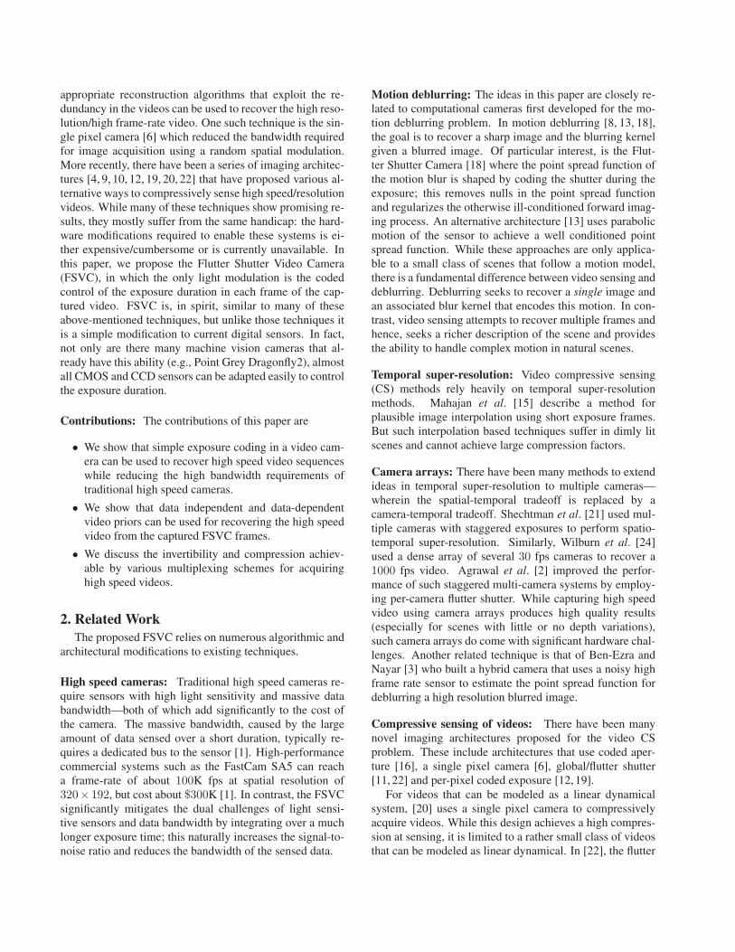
Figure 2. FSVC Architecture: Every captured frame is a sum ofa pseudo-random sampling of sub-frames.

Thus, for FSVC to work reliably, it is pertinent that bothproperties are satisfied and that several successive capturedframes are available during the decoding process. Thisstands in contrast with other methods such as [10] and [12]where motion information can be encoded within a singleframe by independently changing the exposure time for dif-ferent pixels.

3.1. Notation and problem statementLet x be a high speed video of size M×N×T and let xt

be the frame captured at time t. A conventional high speedcamera can capture x directly, whereas a low speed videocamera cannot capture all of the desired frames in x. There-fore, low speed cameras either resort to a short exposurevideo (in which the resultant frames are sharp, but noisy) orto a full-frame exposure (which results in blurred images).In either case, the resulting video is of size N ×N × (T/c)where c is the temporal sub-sampling factor. In the FSVC,we open and close the shutter using a binary pseudorandomsequence within the exposure duration of each frame. In allthree cases, the observed video frames ytl are related to thehigh speed sub-frames xt as

ytl =

tlc∑t=(tl−1)c+1

S(t)xt + ntl , (1)

where S(t) ∈ {0, 1} is the binary global shutter function, xt

is the sub-frame of x at time t, and ntl is observation noise

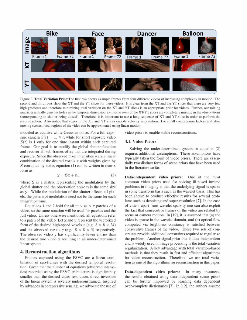
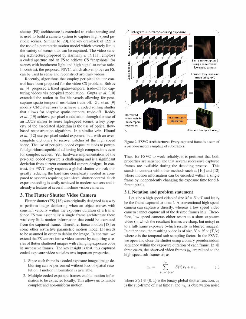
Figure 3. Total Variation Prior:The first row shows example frames from four different videos of increasing complexity in motion. Thesecond and third rows show the XT and the YT slices for these videos. It is clear from the XT and the YT slices that there are very fewhigh gradients and therefore minimizing total variation on the XT and YT slices is an appropriate prior for videos. Further, our mixingmatrix essentially punches holes in the temporal dimension, i.e., some rows of the XT-YT slices are completely missing in the observations(corresponding to shutter being closed). Therefore, it is important to use a long sequence of XT and YT slice in order to perform thereconstruction. Also notice that edges in the XT and YT slices encode velocity information. For small compression factors and slowmoving scenes, local regions of the video can be approximated using linear motion.

modeled as additive white Gaussian noise. For a full expo-sure camera S(t) = 1, ∀ t, while for short exposure videoS(t) is 1 only for one time instant within each capturedframe. Our goal is to modify the global shutter functionand recover all sub-frames of xt that are integrated duringexposure. Since the observed pixel intensities y are a linearcombination of the desired voxels x with weights given byS corrupted by noise, equation (1) can be written in matrixform as

y = Sx+ n, (2)

where S is a matrix representing the modulation by theglobal shutter and the observation noise n is the same sizeas y. While the modulation of the shutter affects all pix-els, the pattern of modulation need not be the same for eachintegration time.

Equations 1 and 2 hold for all m × m × τ patches of avideo, so the same notation will be used for patches and thefull video. Unless otherwise mentioned, all equations referto a patch of the video. Let x and y represent the vectorizedform of the desired high-speed voxels x (e.g. 8 × 8 × 24)and the observed voxels y (e.g. 8 × 8 × 3) respectively.The observed video y has significantly fewer entries thanthe desired true video x resulting in an under-determinedlinear system.

4. Reconstruction algorithmsFrames captured using the FSVC are a linear com-

bination of sub-frames with the desired temporal resolu-tion. Given that the number of equations (observed intensi-ties) recorded using the FSVC architecture is significantlysmaller than the desired video resolution, direct inversionof the linear system is severely underconstrained. Inspiredby advances in compressive sensing, we advocate the use of

video priors to enable stable reconstructions.

4.1. Video Priors

Solving the under-determined system in equation (2)requires additional assumptions. These assumptions havetypically taken the form of video priors. There are essen-tially two distinct forms of scene priors that have been usedin the literature so far.

Data-independent video priors: One of the mostcommon video priors used for solving ill-posed inverseproblems in imaging is that the underlying signal is sparsein some transform basis such as the wavelet basis. This hasbeen shown to produce effective results for several prob-lems such as denoising and super-resolution [7]. In the caseof video, apart from wavelet-sparsity one can also exploitthe fact that consecutive frames of the video are related byscene or camera motion. In [19], it is assumed that (a) thevideo is sparse in the wavelet domain, and (b) optical flowcomputed via brightness constancy is satisfied betweenconsecutive frames of the video. These two sets of con-straints provide additional constraints required to regularizethe problem. Another signal prior that is data-independentand is widely used in image processing is the total variationregularization. A key advantage with total variation-basedmethods is that they result in fast and efficient algorithmsfor video reconstruction. Therefore, we use total varia-tion as one of the algorithms for reconstruction in this paper.

Data-dependent video priors: In many instances,the results obtained using data-independent scene priorscan be further improved by learning data dependentover-complete dictionaries [7]. In [12], the authors assume

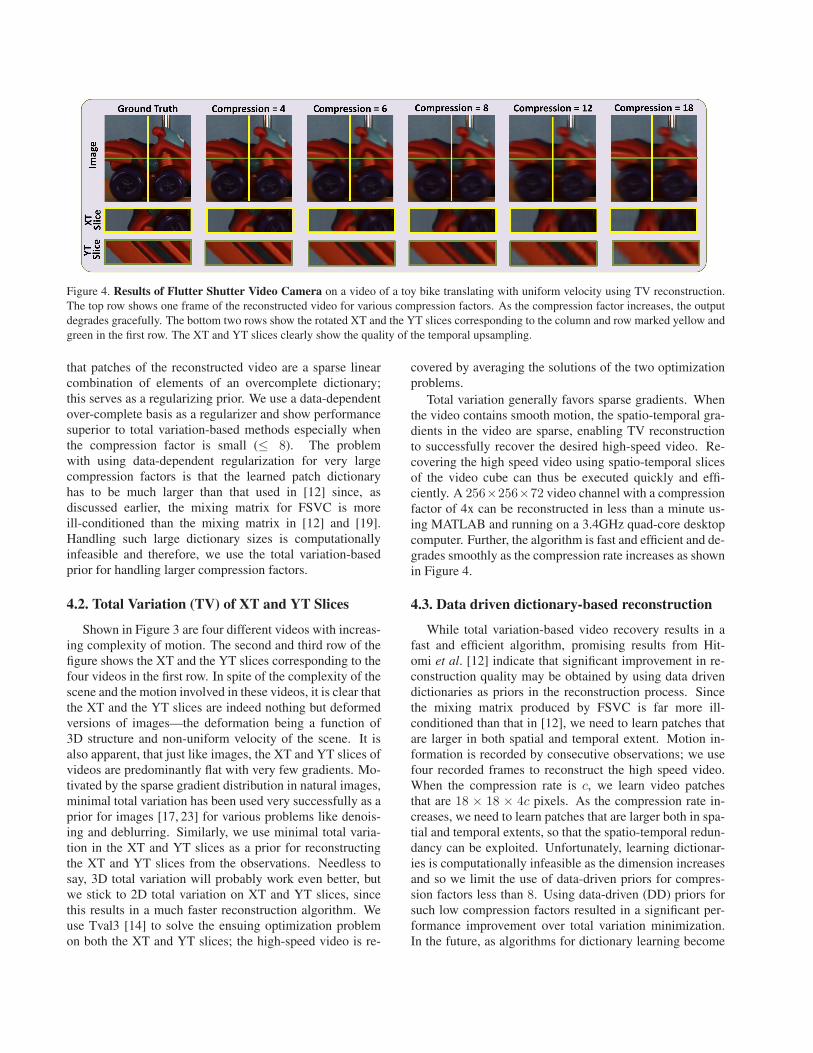
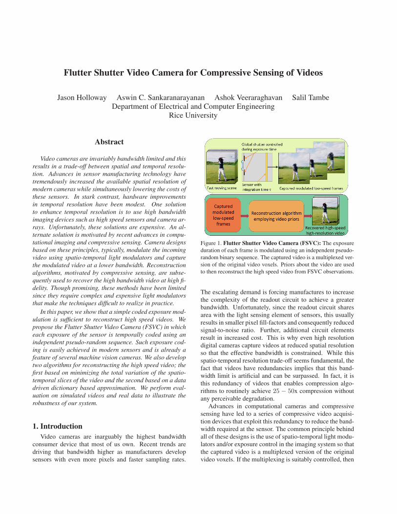
Figure 4. Results of Flutter Shutter Video Camera on a video of a toy bike translating with uniform velocity using TV reconstruction.The top row shows one frame of the reconstructed video for various compression factors. As the compression factor increases, the outputdegrades gracefully. The bottom two rows show the rotated XT and the YT slices corresponding to the column and row marked yellow andgreen in the first row. The XT and YT slices clearly show the quality of the temporal upsampling.

that patches of the reconstructed video are a sparse linearcombination of elements of an overcomplete dictionary;this serves as a regularizing prior. We use a data-dependentover-complete basis as a regularizer and show performancesuperior to total variation-based methods especially whenthe compression factor is small (≤ 8). The problemwith using data-dependent regularization for very largecompression factors is that the learned patch dictionaryhas to be much larger than that used in [12] since, asdiscussed earlier, the mixing matrix for FSVC is moreill-conditioned than the mixing matrix in [12] and [19].Handling such large dictionary sizes is computationallyinfeasible and therefore, we use the total variation-basedprior for handling larger compression factors.

4.2. Total Variation (TV) of XT and YT Slices

Shown in Figure 3 are four different videos with increas-ing complexity of motion. The second and third row of thefigure shows the XT and the YT slices corresponding to thefour videos in the first row. In spite of the complexity of thescene and the motion involved in these videos, it is clear thatthe XT and the YT slices are indeed nothing but deformedversions of images—the deformation being a function of3D structure and non-uniform velocity of the scene. It isalso apparent, that just like images, the XT and YT slices ofvideos are predominantly flat with very few gradients. Mo-tivated by the sparse gradient distribution in natural images,minimal total variation has been used very successfully as aprior for images [17, 23] for various problems like denois-ing and deblurring. Similarly, we use minimal total varia-tion in the XT and YT slices as a prior for reconstructingthe XT and YT slices from the observations. Needless tosay, 3D total variation will probably work even better, butwe stick to 2D total variation on XT and YT slices, sincethis results in a much faster reconstruction algorithm. Weuse Tval3 [14] to solve the ensuing optimization problemon both the XT and YT slices; the high-speed video is re-

covered by averaging the solutions of the two optimizationproblems.

Total variation generally favors sparse gradients. Whenthe video contains smooth motion, the spatio-temporal gra-dients in the video are sparse, enabling TV reconstructionto successfully recover the desired high-speed video. Re-covering the high speed video using spatio-temporal slicesof the video cube can thus be executed quickly and effi-ciently. A 256×256×72 video channel with a compressionfactor of 4x can be reconstructed in less than a minute us-ing MATLAB and running on a 3.4GHz quad-core desktopcomputer. Further, the algorithm is fast and efficient and de-grades smoothly as the compression rate increases as shownin Figure 4.

4.3. Data driven dictionary-based reconstruction

While total variation-based video recovery results in afast and efficient algorithm, promising results from Hit-omi et al. [12] indicate that significant improvement in re-construction quality may be obtained by using data drivendictionaries as priors in the reconstruction process. Sincethe mixing matrix produced by FSVC is far more ill-conditioned than that in [12], we need to learn patches thatare larger in both spatial and temporal extent. Motion in-formation is recorded by consecutive observations; we usefour recorded frames to reconstruct the high speed video.When the compression rate is c, we learn video patchesthat are 18 × 18 × 4c pixels. As the compression rate in-creases, we need to learn patches that are larger both in spa-tial and temporal extents, so that the spatio-temporal redun-dancy can be exploited. Unfortunately, learning dictionar-ies is computationally infeasible as the dimension increasesand so we limit the use of data-driven priors for compres-sion factors less than 8. Using data-driven (DD) priors forsuch low compression factors resulted in a significant per-formance improvement over total variation minimization.In the future, as algorithms for dictionary learning become

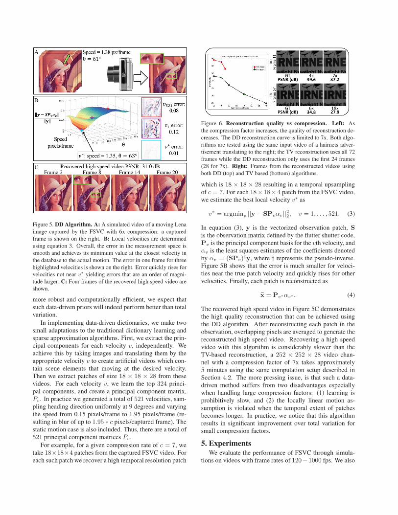
Figure 5. DD Algorithm. A: A simulated video of a moving Lenaimage captured by the FSVC with 6x compression; a capturedframe is shown on the right. B: Local velocities are determinedusing equation 3. Overall, the error in the measurement space issmooth and achieves its minimum value at the closest velocity inthe database to the actual motion. The error in one frame for threehighlighted velocities is shown on the right. Error quickly rises forvelocities not near v∗ yielding errors that are an order of magni-tude larger. C: Four frames of the recovered high speed video areshown.

more robust and computationally efficient, we expect thatsuch data-driven priors will indeed perform better than totalvariation.

In implementing data-driven dictionaries, we make twosmall adaptations to the traditional dictionary learning andsparse approximation algorithms. First, we extract the prin-cipal components for each velocity v, independently. Weachieve this by taking images and translating them by theappropriate velocity v to create artificial videos which con-tain scene elements that moving at the desired velocity.Then we extract patches of size 18 × 18 × 28 from thesevideos. For each velocity v, we learn the top 324 princi-pal components, and create a principal component matrix,Pv . In practice we generated a total of 521 velocities, sam-pling heading direction uniformly at 9 degrees and varyingthe speed from 0.15 pixels/frame to 1.95 pixels/frame (re-sulting in blur of up to 1.95 ∗ c pixels/captured frame). Thestatic motion case is also included. Thus, there are a total of521 principal component matrices Pv .

For example, for a given compression rate of c = 7, wetake 18×18×4 patches from the captured FSVC video. Foreach such patch we recover a high temporal resolution patch

Figure 6. Reconstruction quality vs compression. Left: Asthe compression factor increases, the quality of reconstruction de-creases. The DD reconstruction curve is limited to 7x. Both algo-rithms are tested using the same input video of a hairnets adver-tisement translating to the right; the TV reconstruction uses all 72frames while the DD reconstruction only uses the first 24 frames(28 for 7x). Right: Frames from the reconstructed videos usingboth DD (top) and TV based (bottom) algorithms.

which is 18 × 18 × 28 resulting in a temporal upsamplingof c = 7. For each 18× 18× 4 patch from the FSVC video,we estimate the best local velocity v∗ as

v∗ = argminv ||y − SPvαv||22, v = 1, . . . , 521. (3)

In equation (3), y is the vectorized observation patch, Sis the observation matrix defined by the flutter shutter code,Pv is the principal component basis for the vth velocity, andαv is the least squares estimates of the coefficients denotedby αv = (SPv)

†y, where † represents the pseudo-inverse.Figure 5B shows that the error is much smaller for veloci-ties near the true patch velocity and quickly rises for othervelocities. Finally, each patch is reconstructed as

x̂ = Pv∗αv∗ . (4)

The recovered high speed video in Figure 5C demonstratesthe high quality reconstruction that can be achieved usingthe DD algorithm. After reconstructing each patch in theobservation, overlapping pixels are averaged to generate thereconstructed high speed video. Recovering a high speedvideo with this algorithm is considerably slower than theTV-based reconstruction, a 252 × 252 × 28 video chan-nel with a compression factor of 7x takes approximately5 minutes using the same computation setup described inSection 4.2. The more pressing issue, is that such a data-driven method suffers from two disadvantages especiallywhen handling large compression factors: (1) learning isprohibitively slow, and (2) the locally linear motion as-sumption is violated when the temporal extent of patchesbecomes longer. In practice, we notice that this algorithmresults in significant improvement over total variation forsmall compression factors.

5. ExperimentsWe evaluate the performance of FSVC through simula-

tions on videos with frame rates of 120−1000 fps. We also

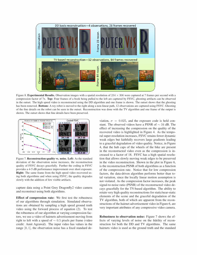
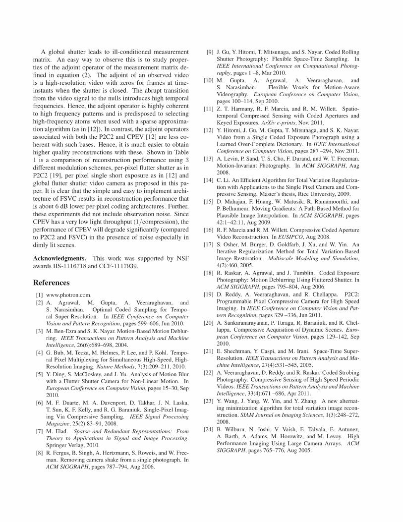
Figure 8. Experimental Results. Observation images with a spatial resolution of 234× 306 were captured at 7 frames per second with acompression factor of 7x. Top: Four frames of a book being pulled to the left are captured by FSVC, ghosting artifacts can be observedin the outset. The high speed video is reconstructed using the DD algorithm and one frame is shown. The outset shows that the ghostinghas been removed. Bottom: A toy robot is moved to the right along a non-linear path, 12 observations are captured using FSVC. Ghostingof the fine details on the robot can be seen in the outset. Reconstruction was done with the TV algorithm and one frame of the output isshown. The outset shows that fine details have been preserved.

Figure 7. Reconstruction quality vs. noise. Left: As the standarddeviation of the observation noise increases, the reconstructionquality of FSVC decays gracefully. Further the coding in FSVCprovides a 4-5 dB performance improvement over short exposure.Right: The same frame from the high speed video recovered us-ing both algorithms and when using FSVC; the quality degradesslowly with the addition of few visible artifacts.

capture data using a Point Grey Dragonfly2 video cameraand reconstruct using both algorithms.

Effect of compression rate: We first test the robustnessof our algorithms through simulation. Simulated observa-tions are obtained by sampling a high speed ground truthvideo using the forward process of equation (2). To testthe robustness of our algorithm at varying compression fac-tors, we use a video of hairnets advertisement moving fromright to left with a speed of ∼ 0.5 pixels per frame (videocredit: Amit Agrawal). The input video has values in therange [0, 1], the observation noise has a fixed standard de-

viation, σ = 0.025, and the exposure code is held con-stant. The observed videos have a PSNR of ∼ 34 dB. Theeffect of increasing the compression on the quality of therecovered video is highlighted in Figure 4. As the tempo-ral super-resolution increases, FSVC retains fewer dynamicweak edges but faithfully recovers large gradients leadingto a graceful degradation of video quality. Notice, in Figure4, that the hub caps of the wheels of the bike are presentin the reconstructed video even as the compression is in-creased to a factor of 18. FSVC has a high spatial resolu-tion that allows slowly moving weak edges to be preservedin the video reconstruction. Shown in the plot in Figure 6,is the reconstruction PSNR of both algorithms as a functionof the compression rate. Notice that for low compressionfactors, the data-driven algorithm performs better than to-tal variation, since the locally linear motion assumption isnot violated. As the compression factor increases, the peaksignal-to-noise ratio (PSNR) of the reconstructed video de-cays gracefully for the TV-based algorithm. The ability toretain very high quality reconstructions for static/near-staticelements of the scene and the graceful degradation of theTV algorithm, both of which are apparent from the recon-structions of the hairnet advertisement video in Figure 6, arevery important attributes of any compressive video camera.

Robustness to observation noise: Figure 7 shows the ef-fects of varying levels of noise on the fidelity of recon-struction for both the DD and TV algorithms. The samehairnets video is used as the ground truth and the standard

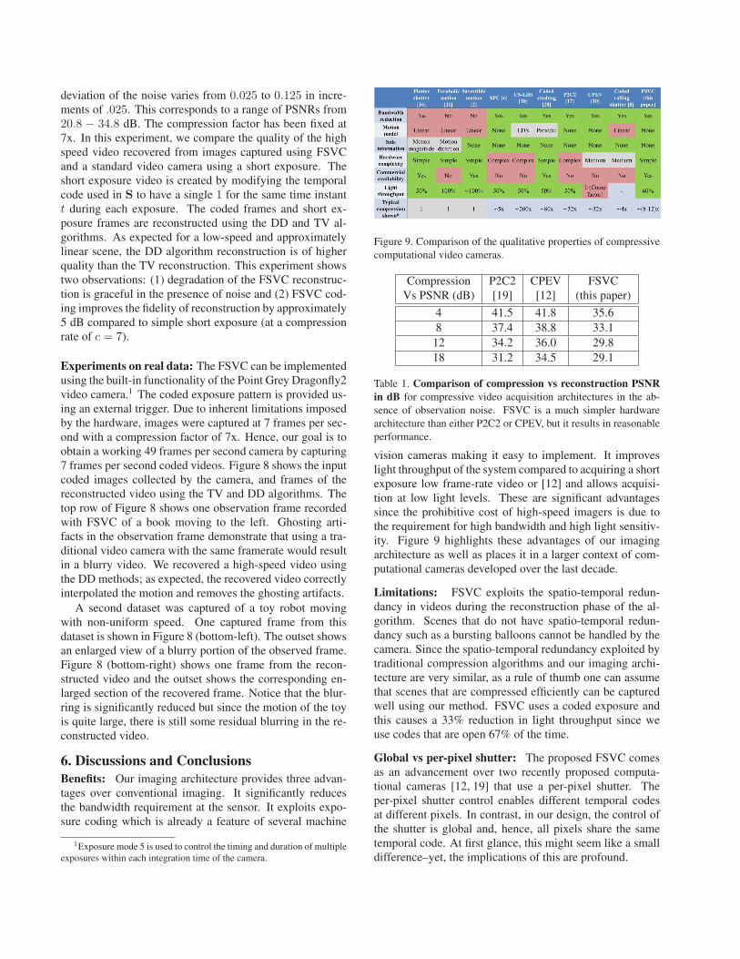
deviation of the noise varies from 0.025 to 0.125 in incre-ments of .025. This corresponds to a range of PSNRs from20.8 − 34.8 dB. The compression factor has been fixed at7x. In this experiment, we compare the quality of the highspeed video recovered from images captured using FSVCand a standard video camera using a short exposure. Theshort exposure video is created by modifying the temporalcode used in S to have a single 1 for the same time instantt during each exposure. The coded frames and short ex-posure frames are reconstructed using the DD and TV al-gorithms. As expected for a low-speed and approximatelylinear scene, the DD algorithm reconstruction is of higherquality than the TV reconstruction. This experiment showstwo observations: (1) degradation of the FSVC reconstruc-tion is graceful in the presence of noise and (2) FSVC cod-ing improves the fidelity of reconstruction by approximately5 dB compared to simple short exposure (at a compressionrate of c = 7).

Experiments on real data: The FSVC can be implementedusing the built-in functionality of the Point Grey Dragonfly2video camera.1 The coded exposure pattern is provided us-ing an external trigger. Due to inherent limitations imposedby the hardware, images were captured at 7 frames per sec-ond with a compression factor of 7x. Hence, our goal is toobtain a working 49 frames per second camera by capturing7 frames per second coded videos. Figure 8 shows the inputcoded images collected by the camera, and frames of thereconstructed video using the TV and DD algorithms. Thetop row of Figure 8 shows one observation frame recordedwith FSVC of a book moving to the left. Ghosting arti-facts in the observation frame demonstrate that using a tra-ditional video camera with the same framerate would resultin a blurry video. We recovered a high-speed video usingthe DD methods; as expected, the recovered video correctlyinterpolated the motion and removes the ghosting artifacts.

A second dataset was captured of a toy robot movingwith non-uniform speed. One captured frame from thisdataset is shown in Figure 8 (bottom-left). The outset showsan enlarged view of a blurry portion of the observed frame.Figure 8 (bottom-right) shows one frame from the recon-structed video and the outset shows the corresponding en-larged section of the recovered frame. Notice that the blur-ring is significantly reduced but since the motion of the toyis quite large, there is still some residual blurring in the re-constructed video.

6. Discussions and ConclusionsBenefits: Our imaging architecture provides three advan-tages over conventional imaging. It significantly reducesthe bandwidth requirement at the sensor. It exploits expo-sure coding which is already a feature of several machine

1Exposure mode 5 is used to control the timing and duration of multipleexposures within each integration time of the camera.

Figure 9. Comparison of the qualitative properties of compressivecomputational video cameras.

Compression P2C2 CPEV FSVCVs PSNR (dB) [19] [12] (this paper)

4 41.5 41.8 35.68 37.4 38.8 33.1

12 34.2 36.0 29.818 31.2 34.5 29.1

Table 1. Comparison of compression vs reconstruction PSNRin dB for compressive video acquisition architectures in the ab-sence of observation noise. FSVC is a much simpler hardwarearchitecture than either P2C2 or CPEV, but it results in reasonableperformance.

vision cameras making it easy to implement. It improveslight throughput of the system compared to acquiring a shortexposure low frame-rate video or [12] and allows acquisi-tion at low light levels. These are significant advantagessince the prohibitive cost of high-speed imagers is due tothe requirement for high bandwidth and high light sensitiv-ity. Figure 9 highlights these advantages of our imagingarchitecture as well as places it in a larger context of com-putational cameras developed over the last decade.

Limitations: FSVC exploits the spatio-temporal redun-dancy in videos during the reconstruction phase of the al-gorithm. Scenes that do not have spatio-temporal redun-dancy such as a bursting balloons cannot be handled by thecamera. Since the spatio-temporal redundancy exploited bytraditional compression algorithms and our imaging archi-tecture are very similar, as a rule of thumb one can assumethat scenes that are compressed efficiently can be capturedwell using our method. FSVC uses a coded exposure andthis causes a 33% reduction in light throughput since weuse codes that are open 67% of the time.

Global vs per-pixel shutter: The proposed FSVC comesas an advancement over two recently proposed computa-tional cameras [12, 19] that use a per-pixel shutter. Theper-pixel shutter control enables different temporal codesat different pixels. In contrast, in our design, the control ofthe shutter is global and, hence, all pixels share the sametemporal code. At first glance, this might seem like a smalldifference–yet, the implications of this are profound.

A global shutter leads to ill-conditioned measurementmatrix. An easy way to observe this is to study proper-ties of the adjoint operator of the measurement matrix de-fined in equation (2). The adjoint of an observed videois a high-resolution video with zeros for frames at time-instants when the shutter is closed. The abrupt transitionfrom the video signal to the nulls introduces high temporalfrequencies. Hence, the adjoint operator is highly coherentto high frequency patterns and is predisposed to selectinghigh-frequency atoms when used with a sparse approxima-tion algorithm (as in [12]). In contrast, the adjoint operatorsassociated with both the P2C2 and CPEV [12] are less co-herent with such bases. Hence, it is much easier to obtainhigher quality reconstructions with these. Shown in Table1 is a comparison of reconstruction performance using 3different modulation schemes, per-pixel flutter shutter as inP2C2 [19], per pixel single short exposure as in [12] andglobal flutter shutter video camera as proposed in this pa-per. It is clear that the simple and easy to implement archi-tecture of FSVC results in reconstruction performance thatis about 6 dB lower per-pixel coding architectures. Further,these experiments did not include observation noise. SinceCPEV has a very low light throughput (1/compression), theperformance of CPEV will degrade significantly (comparedto P2C2 and FSVC) in the presence of noise especially indimly lit scenes.

Acknowledgments. This work was supported by NSFawards IIS-1116718 and CCF-1117939.

References

[1] www.photron.com.[2] A. Agrawal, M. Gupta, A. Veeraraghavan, and

S. Narasimhan. Optimal Coded Sampling for Tempo-ral Super-Resolution. In IEEE Conference on ComputerVision and Pattern Recognition, pages 599–606, Jun 2010.

[3] M. Ben-Ezra and S. K. Nayar. Motion-Based Motion Deblur-ring. IEEE Transactions on Pattern Analysis and MachineIntelligence, 26(6):689–698, 2004.

[4] G. Bub, M. Tecza, M. Helmes, P. Lee, and P. Kohl. Tempo-ral Pixel Multiplexing for Simultaneous High-Speed, High-Resolution Imaging. Nature Methods, 7(3):209–211, 2010.

[5] Y. Ding, S. McCloskey, and J. Yu. Analysis of Motion Blurwith a Flutter Shutter Camera for Non-Linear Motion. InEuropean Conference on Computer Vision, pages 15–30, Sep2010.

[6] M. F. Duarte, M. A. Davenport, D. Takhar, J. N. Laska,T. Sun, K. F. Kelly, and R. G. Baraniuk. Single-Pixel Imag-ing Via Compressive Sampling. IEEE Signal ProcessingMagazine, 25(2):83–91, 2008.

[7] M. Elad. Sparse and Redundant Representations: FromTheory to Applications in Signal and Image Processing.Springer Verlag, 2010.

[8] R. Fergus, B. Singh, A. Hertzmann, S. Roweis, and W. Free-man. Removing camera shake from a single photograph. InACM SIGGRAPH, pages 787–794, Aug 2006.

[9] J. Gu, Y. Hitomi, T. Mitsunaga, and S. Nayar. Coded RollingShutter Photography: Flexible Space-Time Sampling. InIEEE International Conference on Computational Photog-raphy, pages 1 –8, Mar 2010.

[10] M. Gupta, A. Agrawal, A. Veeraraghavan, andS. Narasimhan. Flexible Voxels for Motion-AwareVideography. European Conference on Computer Vision,pages 100–114, Sep 2010.

[11] Z. T. Harmany, R. F. Marcia, and R. M. Willett. Spatio-temporal Compressed Sensing with Coded Apertures andKeyed Exposures. ArXiv e-prints, Nov. 2011.

[12] Y. Hitomi, J. Gu, M. Gupta, T. Mitsunaga, and S. K. Nayar.Video from a Single Coded Exposure Photograph using aLearned Over-Complete Dictionary. In IEEE InternationalConference on Computer Vision, pages 287 –294, Nov 2011.

[13] A. Levin, P. Sand, T. S. Cho, F. Durand, and W. T. Freeman.Motion-Invariant Photography. In ACM SIGGRAPH, Aug2008.

[14] C. Li. An Efficient Algorithm for Total Variation Regulariza-tion with Applications to the Single Pixel Camera and Com-pressive Sensing. Master’s thesis, Rice University, 2009.

[15] D. Mahajan, F. Huang, W. Matusik, R. Ramamoorthi, andP. Belhumeur. Moving Gradients: A Path-Based Method forPlausible Image Interpolation. In ACM SIGGRAPH, pages42:1–42:11, Aug 2009.

[16] R. F. Marcia and R. M. Willett. Compressive Coded ApertureVideo Reconstruction. In EUSIPCO, Aug 2008.

[17] S. Osher, M. Burger, D. Goldfarb, J. Xu, and W. Yin. AnIterative Regularization Method for Total Variation-BasedImage Restoration. Multiscale Modeling and Simulation,4(2):460, 2005.

[18] R. Raskar, A. Agrawal, and J. Tumblin. Coded ExposurePhotography: Motion Deblurring Using Fluttered Shutter. InACM SIGGRAPH, pages 795–804, Aug 2006.

[19] D. Reddy, A. Veeraraghavan, and R. Chellappa. P2C2:Programmable Pixel Compressive Camera for High SpeedImaging. In IEEE Conference on Computer Vision and Pat-tern Recognition, pages 329 –336, Jun 2011.

[20] A. Sankaranarayanan, P. Turaga, R. Baraniuk, and R. Chel-lappa. Compressive Acquisition of Dynamic Scenes. Euro-pean Conference on Computer Vision, pages 129–142, Sep2010.

[21] E. Shechtman, Y. Caspi, and M. Irani. Space-Time Super-Resolution. IEEE Transactions on Pattern Analysis and Ma-chine Intelligence, 27(4):531–545, 2005.

[22] A. Veeraraghavan, D. Reddy, and R. Raskar. Coded StrobingPhotography: Compressive Sensing of High Speed PeriodicVideos. IEEE Transactions on Pattern Analysis and MachineIntelligence, 33(4):671 –686, Apr 2011.

[23] Y. Wang, J. Yang, W. Yin, and Y. Zhang. A new alternat-ing minimization algorithm for total variation image recon-struction. SIAM Journal on Imaging Sciences, 1(3):248–272,2008.

[24] B. Wilburn, N. Joshi, V. Vaish, E. Talvala, E. Antunez,A. Barth, A. Adams, M. Horowitz, and M. Levoy. HighPerformance Imaging Using Large Camera Arrays. ACMSIGGRAPH, pages 765–776, Aug 2005.