PATH PLANNING AND EVOLUTIONARY OPTIMIZATION OF
WHEELED ROBOTS
DALJEET SINGH
Bachelor of Science in Computer Engineering
Cleveland State University
May 2011
A thesis submitted in partial fulfillment of the requirements for the degree of
MASTERS OF SCIENCE IN ELECTRICAL ENGINEERING
at the
Cleveland State University
May 2013
This thesis has been approved for the
Department of Electrical and Computer Engineering
and the college of Graduate Studies by
Thesis Committee Chairperson, Dr. Dan Simon
Department/Date
Dr. Nigamanth Sridhar
Department/Date
Dr. Chansu Yu
Department/Date

ACKNOWLEDGEMENT
I would like to thank my advisor Dr. Simon for his continuous support and assistance
throughout this research. In addition thanks for being my mentor and advisor for my
academic career at Cleveland State University. I would also like to thank the other thesis
committee members, Dr. Nigamanth Sridhar and Dr. Chansu Yu, for their willingness to
be on the committee. I would also like to thank my fellow students in the embedded lab
for creating a friendly and motivating environment while working on this thesis. I would
like to thank the students who built the robot in 2007 which was used for testing the
results of this thesis. Finally, I would like to thank my family and friends for their support
and patience.
iv
PATH PLANNING AND EVOLUTIONARY OPTIMIZATION OF WHEELED
ROBOTS
DALJEET SINGH
ABSTRACT
Probabilistic roadmap methods (PRM) have been a well-known solution for solving
motion planning problems where we have a fixed set of start and goal configurations in
a workspace. We define a configuration space with static obstacles. We implement PRM
to find a feasible path between start and goal for car-like robots. We further extend the
concept of path planning by incorporating evolutionary optimization algorithms to tune
the PRM parameters. The theory is demonstrated with simulations and experiments.
Our results show that there is a significant improvement in the performance metrics of
PRM after optimizing the PRM parameters using biogeography-based optimization,
which is an evolutionary optimization algorithm. The performance metrics (namely path
length, number of hops, number of loops and fail-rate) show 34.91%, 23.18%, 52.21%
and 21.21% improvement after using optimized PRM parameters. We also
experimentally demonstrate the application of path planning using PRM to mobile car-
like robots.
v
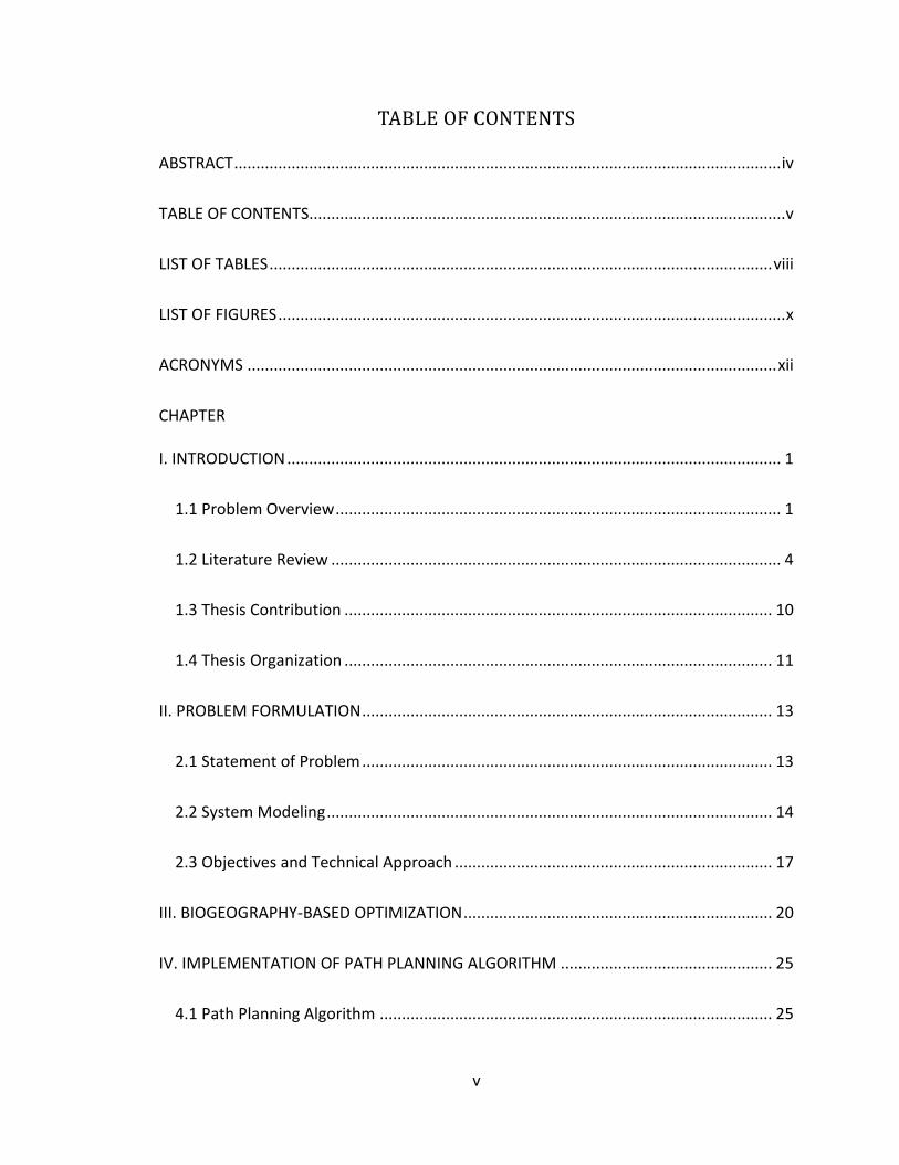
TABLE OF CONTENTS
ABSTRACT ............................................................................................................................ iv
TABLE OF CONTENTS............................................................................................................ v
LIST OF TABLES .................................................................................................................. viii
LIST OF FIGURES ................................................................................................................... x
ACRONYMS ........................................................................................................................ xii
CHAPTER
I. INTRODUCTION ................................................................................................................ 1
1.1 Problem Overview ..................................................................................................... 1
1.2 Literature Review ...................................................................................................... 4
1.3 Thesis Contribution ................................................................................................. 10
1.4 Thesis Organization ................................................................................................. 11
II. PROBLEM FORMULATION ............................................................................................. 13
2.1 Statement of Problem ............................................................................................. 13
2.2 System Modeling ..................................................................................................... 14
2.3 Objectives and Technical Approach ........................................................................ 17
III. BIOGEOGRAPHY-BASED OPTIMIZATION ...................................................................... 20
IV. IMPLEMENTATION OF PATH PLANNING ALGORITHM ................................................ 25
4.1 Path Planning Algorithm ......................................................................................... 25
vi
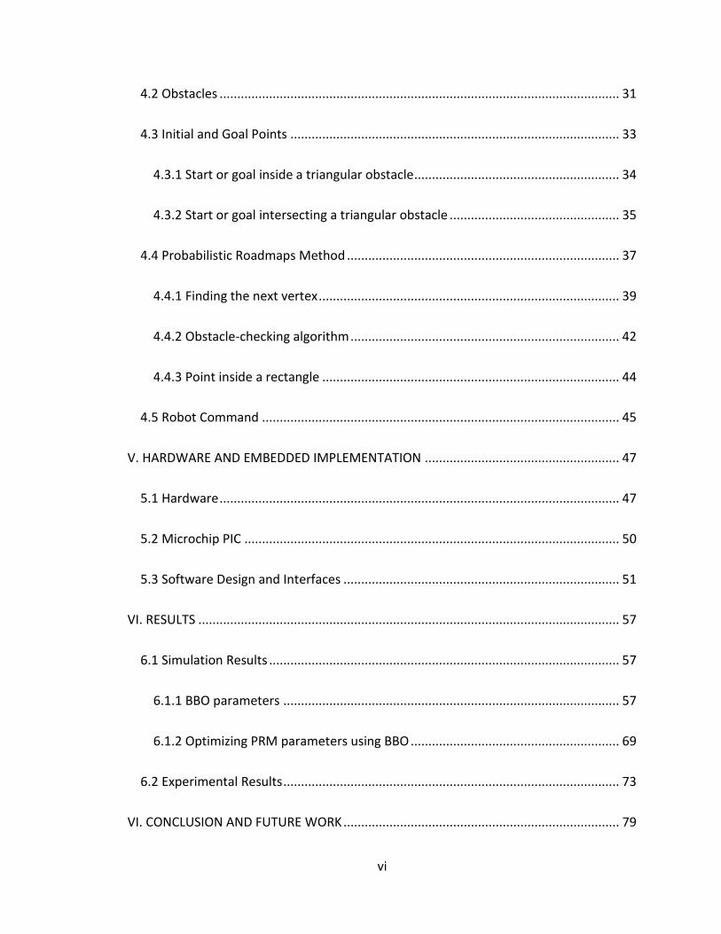
4.2 Obstacles ................................................................................................................. 31
4.3 Initial and Goal Points ............................................................................................. 33
4.3.1 Start or goal inside a triangular obstacle .......................................................... 34
4.3.2 Start or goal intersecting a triangular obstacle ................................................ 35
4.4 Probabilistic Roadmaps Method ............................................................................. 37
4.4.1 Finding the next vertex ..................................................................................... 39
4.4.2 Obstacle-checking algorithm ............................................................................ 42
4.4.3 Point inside a rectangle .................................................................................... 44
4.5 Robot Command ..................................................................................................... 45
V. HARDWARE AND EMBEDDED IMPLEMENTATION ....................................................... 47
5.1 Hardware ................................................................................................................. 47
5.2 Microchip PIC .......................................................................................................... 50
5.3 Software Design and Interfaces .............................................................................. 51
VI. RESULTS ....................................................................................................................... 57
6.1 Simulation Results ................................................................................................... 57
6.1.1 BBO parameters ............................................................................................... 57
6.1.2 Optimizing PRM parameters using BBO ........................................................... 69
6.2 Experimental Results ............................................................................................... 73
VI. CONCLUSION AND FUTURE WORK .............................................................................. 79
vii
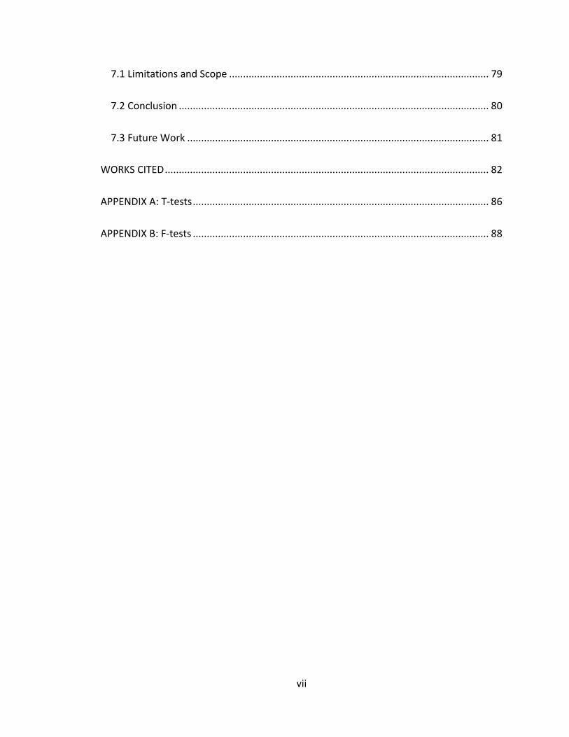
7.1 Limitations and Scope ............................................................................................. 79
7.2 Conclusion ............................................................................................................... 80
7.3 Future Work ............................................................................................................ 81
WORKS CITED .................................................................................................................... 82
APPENDIX A: T-tests .......................................................................................................... 86
APPENDIX B: F-tests .......................................................................................................... 88
viii
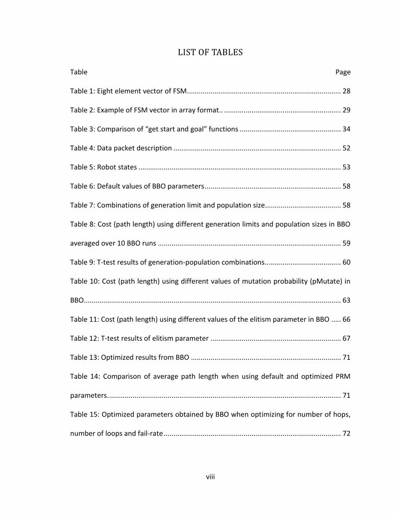
LIST OF TABLES
Table Page
Table 1: Eight element vector of FSM ............................................................................... 28
Table 2: Example of FSM vector in array format.. ............................................................ 29
Table 3: Comparison of “get start and goal” functions .................................................... 34
Table 4: Data packet description ...................................................................................... 52
Table 5: Robot states ........................................................................................................ 53
Table 6: Default values of BBO parameters ...................................................................... 58
Table 7: Combinations of generation limit and population size....................................... 58
Table 8: Cost (path length) using different generation limits and population sizes in BBO
averaged over 10 BBO runs .............................................................................................. 59
Table 9: T-test results of generation-population combinations.. ..................................... 60
Table 10: Cost (path length) using different values of mutation probability (pMutate) in
BBO.................................................................................................................................... 63
Table 11: Cost (path length) using different values of the elitism parameter in BBO ..... 66
Table 12: T-test results of elitism parameter ................................................................... 67
Table 13: Optimized results from BBO ............................................................................. 71
Table 14: Comparison of average path length when using default and optimized PRM
parameters. ....................................................................................................................... 71
Table 15: Optimized parameters obtained by BBO when optimizing for number of hops,
number of loops and fail-rate ........................................................................................... 72

ix
Table 16: Cost values when using default PRM parameters, and when using BBO-
optimized PRM parameters. ............................................................................................. 72
Table 17: Output of PRM using input parameters optimized for path length ................. 73
Table 18: Vertex-edge array and angle of rotation from PRM ......................................... 75
x
LIST OF FIGURES
Figure Page
Figure 1: Robot path planning using PRM.. ........................................................................ 3
Figure 2: Algorithm to construct roadmap [2] .................................................................... 6
Figure 3: Possible directions for robot movement ........................................................... 14
Figure 4: Flow chart of system model ............................................................................... 17
Figure 5: Species model of a single habitat [20] ............................................................... 22
Figure 6: Window angle and bias ...................................................................................... 26
Figure 7: Bias towards or away from the goal .................................................................. 28
Figure 8: Example of FSM vector in graphical format with probabilities of each state.. . 29
Figure 9: Pre-defined test obstacles ................................................................................. 32
Figure 10: Triangular obstacle ABC and point X ............................................................... 35
Figure 11: Circle-triangle intersection points. .................................................................. 36
Figure 12: Generalized PRM main loop. ........................................................................... 38
Figure 13: Next vertex based on horizontal axis............................................................... 40
Figure 14: Next vertex angle based on fixed angle ........................................................... 41
Figure 15: Next vertex based on variable window angle.................................................. 42
Figure 16: Extended next vertices .................................................................................... 43
Figure 17: Robot going over an obstacle .......................................................................... 44
Figure 18: Point X inside the rectangle ABCD. .................................................................. 45
Figure 19: Printed circuit board used in robot [24] .......................................................... 48
Figure 20: Photograph of MaxStream 9Xtend wireless radio [21] ................................... 49
xi
Figure 21: One of Cleveland State University's mobile robots ......................................... 50
Figure 22: Pin diagram of 40-pin PIC18F4520. Taken from [27] ....................................... 51
Figure 23: Communication between the computer workstation and robot .................... 54
Figure 24: Robot wheels at different velocities [28] ........................................................ 56
Figure 25: Average cost vs. generation limit / population size combinations (20, 20), (40,
10) and (10, 40) ................................................................................................................. 61
Figure 26: Average cost vs. generation limit / population size combinations (40, 10), (50,
8) and (100, 4) ................................................................................................................... 62
Figure 27: Average cost vs. mutation probability – 0.001, 0.01 and 0.1 .......................... 64
Figure 28: Average cost vs. mutation probability – 0.1, 0.2 and 0.3 ................................ 65
Figure 29: Average cost vs. elitism parameter 5, 6 and 7 ................................................. 68
Figure 30: Average cost vs. elitism parameter 6, 7 and 8 ................................................. 69
Figure 31: Average and minimum cost of BBO ................................................................. 70
Figure 32: A sample PRM-generated path from start to goal .......................................... 74
Figure 33: Robot at the start position ............................................................................... 76
Figure 34: Robot at the second vertex while going from (0.5, 0.5) to (2.5, 2.5) .............. 77
Figure 35: Robot getting to the goal point (2.5, 2.5) ........................................................ 78
xii
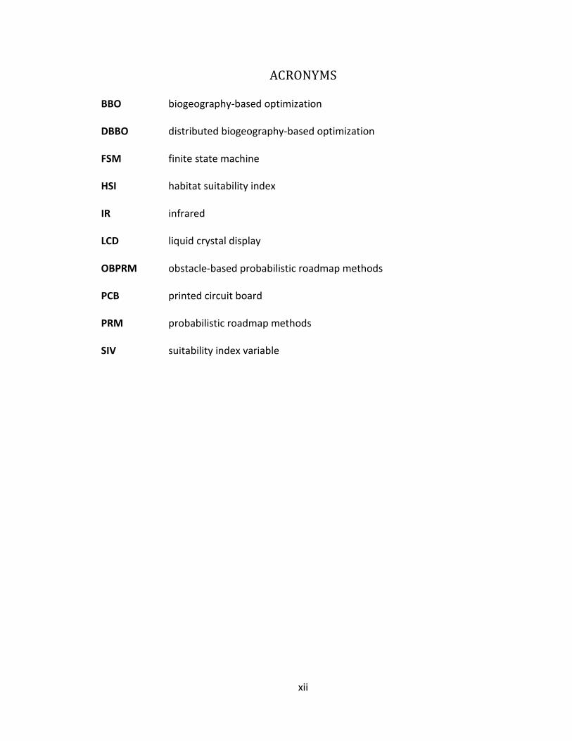
ACRONYMS
BBO biogeography-based optimization
DBBO distributed biogeography-based optimization
FSM finite state machine
HSI habitat suitability index
IR infrared
LCD liquid crystal display
OBPRM obstacle-based probabilistic roadmap methods
PCB printed circuit board
PRM probabilistic roadmap methods
SIV suitability index variable
1
CHAPTER I
INTRODUCTION
This chapter will introduce and provide the preliminary background for the research
work done for this thesis. This chapter covers the problem overview, literature review
and the contribution of this thesis. The preliminaries and the groundwork for this
research are highlighted in brief.
1.1 Problem Overview
There has been a lot of work in robot navigation field in past two decades which
relates directly to improve and enhance the quality of life [1], [2]. There are a number of
different situations or cases for motion planning problems, such as finding a path
between the start and goal in a given scenario, covering the whole area of a
configuration space, or patrolling an area of interest [3]. Robot automation enables our
society to finish more tasks in a given time. Robot automation provides us with the
2
benefit of using robots for jobs such as snow plowing, oceanographic imaging, taking
pictures of an area with radioactivity problems, space exploration and many more [1].
This leads to a need of developing successful robot navigation algorithms. Many
algorithms have been developed to tackle this problem of robot path planning. The field
of study addressed in this thesis is to optimize these robot navigation algorithms for the
best performance over a set of pre-defined metrics.
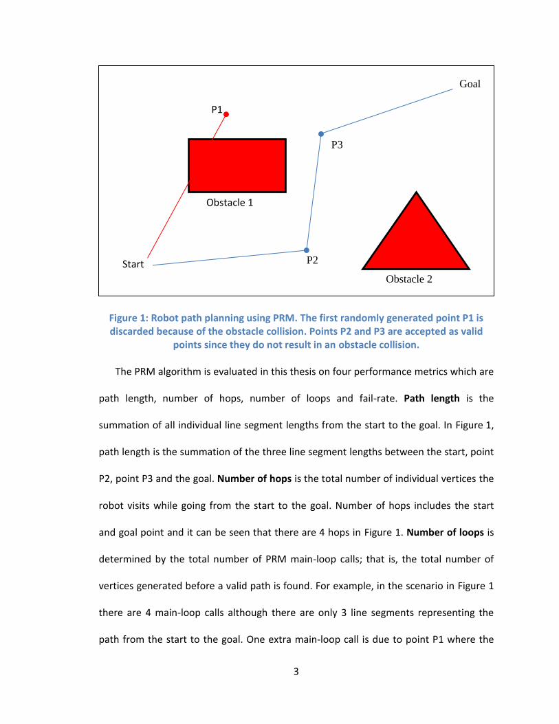
Figure 1 shows an example of robot path planning using PRM. We have a
configuration space with two obstacles as illustrated by the rectangle and the triangle.
Our goal is to find a feasible path between the start and goal points. PRM finds a
random point P1 in the configuration space. An obstacle check then determines that line
segment between the start and P1 intersects with the obstacle. PRM therefore ignores
point P1 and finds a new random point P2, which turns out to be in free space. P2 is
therefore added as the next vertex and the algorithm is repeated until the robot reaches
the goal.
3
Figure 1: Robot path planning using PRM. The first randomly generated point P1 is discarded because of the obstacle collision. Points P2 and P3 are accepted as valid
points since they do not result in an obstacle collision.
The PRM algorithm is evaluated in this thesis on four performance metrics which are
path length, number of hops, number of loops and fail-rate. Path length is the
summation of all individual line segment lengths from the start to the goal. In Figure 1,
path length is the summation of the three line segment lengths between the start, point
P2, point P3 and the goal. Number of hops is the total number of individual vertices the
robot visits while going from the start to the goal. Number of hops includes the start
and goal point and it can be seen that there are 4 hops in Figure 1. Number of loops is
determined by the total number of PRM main-loop calls; that is, the total number of
vertices generated before a valid path is found. For example, in the scenario in Figure 1
there are 4 main-loop calls although there are only 3 line segments representing the
path from the start to the goal. One extra main-loop call is due to point P1 where the
Start
Goal
P1
P2
P3
Obstacle 1
Obstacle 2
4
path was not in free space. Fail-rate is the percentage of PRM evaluations (among
several random robot/obstacle configurations) that fail to find a path to the goal within
N main loop calls, where N is a user-specified limit. For our purposes, this limit was set
to 50. The performance metrics are further discussed in Section 4.1.
1.2 Literature Review
There has been a lot of work done on motion planning in the past two decades.
Algorithms are being developed to tackle these problems in more efficient ways. Some
of the path-planning algorithms for robots are coverage path planning [1] and
probabilistic roadmap methods.
In conventional path planning we have a set of start and goal configurations and the
aim is to find a feasible path between the start and the goal. Coverage path planning, on
the other hand, addresses the problem of finding a path for a robot to cover all possible
points in the free space. This approach can be applied to robotic demining, snow
removal, lawn mowing, painting, mine hunting, harvesting, etc. [1]. The main concern in
this approach is usually the time it takes for the algorithm to cover all the free space in
the configuration space. Clearly, it may take a long time to find a path that covers all the
possible points in the configuration space. Moreover, if the configuration space has
moving obstacles, this problem becomes much more complex and computationally
demanding if PRM is used.
In [4], PRMS is extended and applied to car-like robots. This approach directly relates
to the scope of this thesis where we used car-like robots which can only move forward
(no reverse). The aim of using PRM is to find a feasible path from the start to the goal. In
5
this approach motion planning can be divided into two phases: the learning phase and
the query phase. In the learning phase a probabilistic roadmap is constructed and saved
in a vertex-edge array. In the query phase, this roadmap or vertex-edge array can be
used to find the path between a starting point and a goal point. This approach to path
planning can be successfully applied to car-like robots.
Information about the configuration space can be used to generate samples of
vertices and edges to be saved as a data structure. This information is then used to run
queries to find a path between the start and goal positions. There are a number of ways
and techniques to implement this algorithm. Many different fields are benefitting from
the improvement in motion planning algorithms, including cell structures, computer
graphics, computer assisted surgeries and computer aided design [2], [5], [6], [7], [8].
Some of the variants of PRM, such as lazy PRMs and visibility based PRMs, are examined
in [9].
Reference [2] provides a comparative study of different techniques and ideas used
to implement PRMs. However, it is hard to compare these techniques because of
differences in configuration, differences in testing spaces and differences in hardware.
In general, the motion planning problem proposes the question of computing a path
between two locations. The computed path must be collision-free. Initially the problem
was studied only in the robotics community but recently there has been a broader look
at the problem and its applications. Some of these fields are animation, virtual
environments, gaming and computational chemistry [2].
6
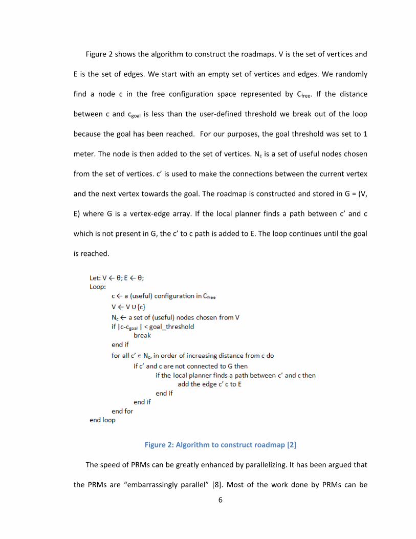
Figure 2 shows the algorithm to construct the roadmaps. V is the set of vertices and
E is the set of edges. We start with an empty set of vertices and edges. We randomly
find a node c in the free configuration space represented by Cfree. If the distance
between c and cgoal is less than the user-defined threshold we break out of the loop
because the goal has been reached. For our purposes, the goal threshold was set to 1
meter. The node is then added to the set of vertices. Nc is a set of useful nodes chosen
from the set of vertices. c’ is used to make the connections between the current vertex
and the next vertex towards the goal. The roadmap is constructed and stored in G = (V,
E) where G is a vertex-edge array. If the local planner finds a path between c’ and c
which is not present in G, the c’ to c path is added to E. The loop continues until the goal
is reached.
Figure 2: Algorithm to construct roadmap [2]
The speed of PRMs can be greatly enhanced by parallelizing. It has been argued that
the PRMs are “embarrassingly parallel” [8]. Most of the work done by PRMs can be
7
parallelized with little effort. Significant speedups can be achieved by incorporating
parallelization in any randomized motion planning algorithm. It has been noted that the
generation of nodes is very fast compared to making successful connections. On average
PRM spends 2-3% of the time in the learning phase and 97-98% of the time in the query
phase. It is shown that significant speedups are achieved by parallelizing the query
phase. For the simple parallelizing strategy, multiple processors are used to generate
nodes and find the connections simultaneously. The inherent parallelism in PRM
algorithms can easily be exploited to achieve significant and scalable speedups.
There have been a number of variants of PRM. One of the variants which apply to
closed chain systems with high degrees of freedom (DOF) is discussed in [10]. A closed
chain system is formed by multiple robots grasping an object. Degrees of freedom refer
to the number of independent variables that define the movement of a body. Here a
body is a closed-chain system of multiple robots. The robots then work in conjunction
with each other to move the object. Kinematics-based PRM is then applied to the closed
chain in a workspace with obstacles. Dynamic path planning for a robot with high DOF in
complex 3D workspaces is discussed in [5]. The novel feature of evaluating areas which
are in free-space is employed. These areas of the workspace can be assigned to ‘zones’
with different degrees of desirability. For example, a ‘zone’ which is far away from any
obstacle or workspace path will have a higher degree of desirability than a ‘zone’ which
is closer to an obstacle or the border of the workspace. This approach can be used to re-
compute paths in dynamic environments where the obstacles are moving. The quality of
a generated path is improved by using dynamic exploration of the roadmaps. A
8
comparative evaluation of different distance metrics and local planners are discussed in
[11].
An obstacle based PRM (OBPRM) is proposed in [12]. That paper has a novel idea of
generating the candidate nodes by choosing the nodes corresponding to the obstacles in
configuration space. The method can be used for OBPRM only if the change in the
environment is incremental. Various techniques to tackle the components of PRM such
as dynamic collision checking, dealing with narrow passages, multi-goal motion
planning, and manipulation planning for deformable linear objects are discussed in [13].
Path smoothing is also incorporated to optimize the path between a set of nodes in
configuration space. OBPRM is further enhanced for cluttered multi-dimensional
workspaces in [7], [14] and [15].
A different approach of obstacle avoidance in a cluttered dynamic environment is
used in [6]. That approach is incorporated with the search for the shortest path from the
PRM connections or queries. A laser range finder is used to implement obstacle
avoidance. The technique is that the robot starts moving at its full speed following the
shortest path. When an obstacle obstructs the path, the laser range finder instructs the
robot to slow its speed until the path is clear. This strategy saves time because the
learning and query phases are not re-computed when we find a dynamic obstacle
crossing the robot’s path. The point for consideration in this technique is that additional
hardware is needed to fully implement obstacle avoidance. In addition, just slowing the
speed of the robot does not ensure that it will not hit the obstacle.
9
These problems can be addressed by using real-time obstacle detection, which
includes reactive path planning [16]. Traditional PRM with dynamic constraints was
considered to tackle the problem in a real-time dynamic environment. However, the
article suggests that this approach may not be well-suited for real-time
implementations. Rapidly-exploring random trees (RRTs) can effectively solve complex
dynamic motion planning problems. This approach is further enhanced in [17] by a
waypoint cache and adaptive cost penalty, which improves the efficiency of re-planning
the path and the overall quality of generated solutions. This method is called execution
extended rapidly-exploring random trees (ERRT).
Area patrolling by multiple robots with frequency constraints and adversarial
settings is discussed in [3] and [18]. The problem of multi-robot perimeter patrol has
been discussed in [3]. A strong adversary model is implemented which knows the
location and the patrol scheme used by the robots. That paper proposes different
models to find the probability of penetration. The traditional models of robot path
planning only cover the points included in the path. The frequency of any specific point
in the path is ignored. A patrol algorithm is presented in [18] which covers all the points
in the given area with the optimal frequency. Sampling the free configuration space to
get a better coverage of the area is discussed in [19]. A new sampling strategy, Gaussian
sampling, was introduced to tackle difficult areas. It has been proposed that we do not
need a lot of sampling points in open spaces. On the other hand, it is hard to find a good
path in difficult areas such as near the obstacles or the borders of the room. The
strategy proposed in [19] is that we sample more points near the difficult areas as
10
compared to the open areas. The technique has shown improvements in random
sampling tests.
1.3 Thesis Contribution
This thesis contributes to the ongoing development and implementation of robot
path planning algorithms. PRM can be adjusted based on the system specifications and
the workspace. The path planning results, i.e., the set of nodes and edges, can then be
improved by optimizing the parameters of PRM. We successfully optimized PRM using
biogeography-based optimization. This shows that path planning results from algorithms
such as PRM can be optimized and enhanced. It further supports the theory that
biogeography-based optimization can be used to optimize complex mathematical
problems [20]. It shows a direct relation between the biological behavior of living
organisms and man-made machines.
Motion planning is a common problem in robotics. Although there has been a
tremendous amount of work in this field for past two decades, no perfect answer or
algorithm exists. The approach to solve motion planning problems depends on the given
set of parameters and configurations. This thesis covers the implementation and
optimizing of the motion planning algorithm PRM for car-like robots.
We implement the PRM algorithm for car-like robots. The results are backed up by
simulations and experiments. The microcontroller on the robot is programmed to
receive the path from PRM via radio commands. The path is then used to move the car-
like robot from the start to the goal position. The robot follows the feasible path found
by PRM in a configuration space with obstacles.
11
We use biogeography-based optimization to optimize the PRM parameters. A lot of
methods have been proposed to tackle the problem of path planning for car-like robots.
The contribution of this thesis is to show that optimization algorithms can be applied to
path planning algorithms to get better results. The traditional PRM approach can easily
be modified based on configuration-specific parameters and the inputs can be adjusted
according to the specifications.
We used a variant of PRM based on the configuration scenario used by our mobile
robot. Only one query is generated at each point and the results are directly used to find
the goal within the free space. The algorithm to find the next feasible path depends on
the set of PRM parameters.
1.4 Thesis Organization
Chapter II gives a brief overview of the formulation and statement of the robot path
planning problem. It includes system modeling and various approaches for robot
navigation.
Chapter III describes how an evolutionary algorithm such as BBO can be applied to
mathematical problems with a set of discrete parameters. That chapter also describes
how BBO is used to tune the parameters to find better PRM results. That chapter also
illustrates the success of BBO as a black-box optimizer.
Next, we cover the MATLAB functions used in the system simulations. Chapter IV
covers all the major MATLAB functions and their implementation including the pseudo
code and specifications used to simulate the robot world.
12
Chapter V covers the embedded implementation of this project, which includes the
robot and radio hardware used for this thesis. It also includes a brief description of the
software design and implementation.
Chapter VI summarizes the simulation and experimental results. We start with the
PRM simulation results and then describe the statistical tests of optimizing four input
parameters of PRM using BBO. We also demonstrate the hardware result of the robot
following the optimized path generated by PRM.
Chapter VII gives an overview of the findings and the results from this thesis. It also
covers the limitations and scope of this project in an engineering environment. It gives a
brief introduction to the future applications and possibilities for this project. It further
supports the idea presented in [20] to merge the fields of biogeography and engineering
for their mutual benefit.
13
CHAPTER II
PROBLEM FORMULATION
The purpose of this research is to study path planning problems using PRM, to use
new algorithms to optimize PRM and to verify the results in an experimental system.
This chapter introduces the statement of problem (Section 2.1), system modeling
(Section 2.2), and the objectives and technical approach (Section 2.3).
2.1 Statement of Problem
There has been a lot of work in the past for developing a better path planning
algorithm for mobile car-like robots. Over the past decade, probabilistic roadmap
methods have provided good solutions to this problem. However, PRMs can be easily
modified according to the user’s needs.
Traditionally, the approach to enhance PRM or any other path planning algorithm is
by using hardware or computational enhancements. Hardware enhancements can be
made with sensors, encoders, cameras, etc. [6], [12], [16], [20], [21]. Computational
14
enhancements can be made by parallelizing the PRM querying [8]. This thesis presents a
novel and simple idea of tuning the PRM parameters using biogeography-based
optimization.
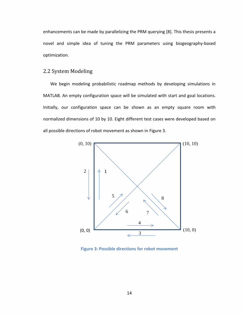
2.2 System Modeling
We begin modeling probabilistic roadmap methods by developing simulations in
MATLAB. An empty configuration space will be simulated with start and goal locations.
Initially, our configuration space can be shown as an empty square room with
normalized dimensions of 10 by 10. Eight different test cases were developed based on
all possible directions of robot movement as shown in Figure 3.
Figure 3: Possible directions for robot movement
(0, 0) (10, 0)
(0, 10) (10, 10)
1 2
5
6 7
8
4
3
15
Possible directions for robot movements as shown in Figure 3 are:
1. Up
2. Down
3. Left
4. Right
5. Diagonally up right
6. Diagonally down left
7. Diagonally up left
8. Diagonally down right
PRM operates by generating a random angle theta. This angle is then used to
determine the direction of motion. After initial testing in an obstacle free configuration
space we added three test obstacles. This led us to add obstacle checking in our
algorithm. PRMs are then adjusted for obstacle checking and ignoring the randomly-
generated nodes that result in the robot hitting an obstacle.
Cartesian coordinates are used for configuration space, obstacles and robot
locations. We use pre-defined knowledge of obstacles to determine whether the next
PRM-determined location is in free space. The robot is represented as a circle and we
test if the circle intersects the sides of the obstacles.
Random start, goal and obstacle configurations were implemented after testing was
done with pre-defined configurations. This allowed our implementation of PRM to be
more robust. It also ensured that the results could be applied to almost any
configuration.
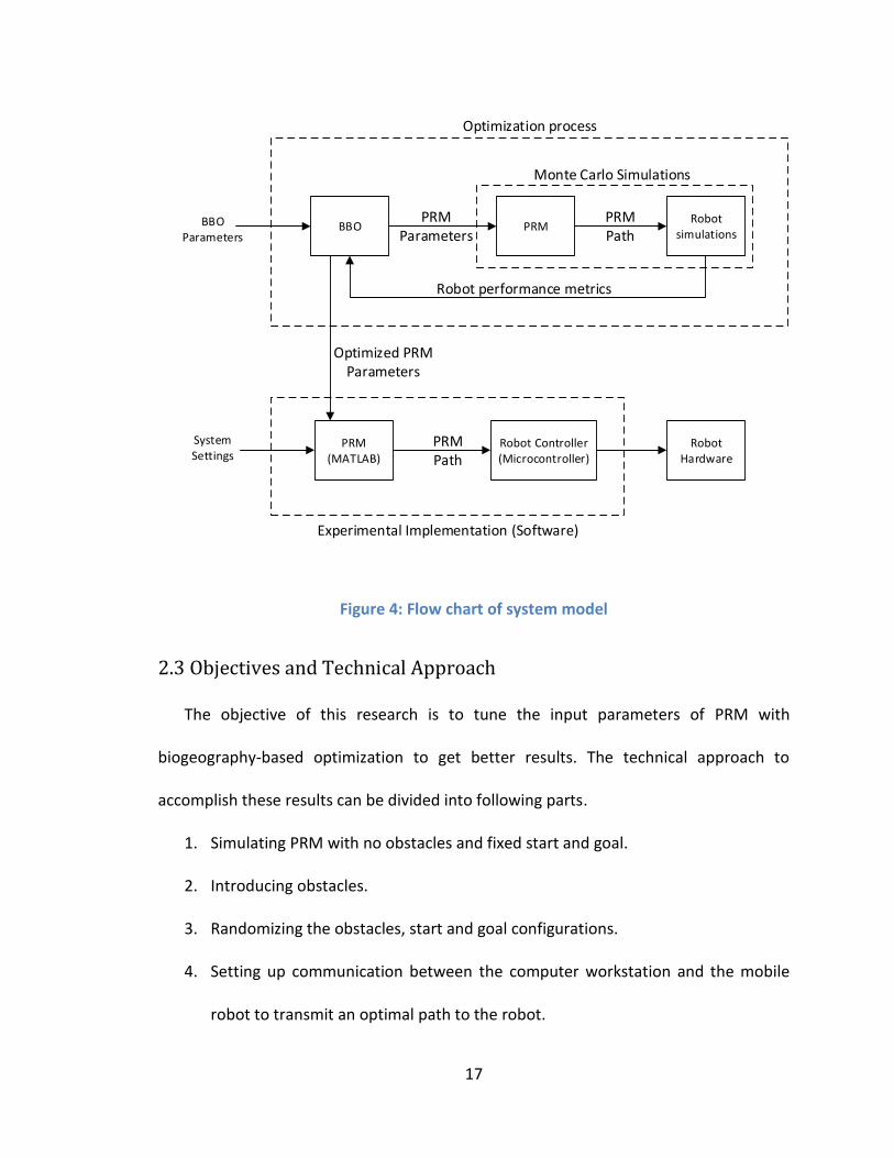
Figure 4 shows the model of the system in three major blocks. The first block
represents the optimization process where we run BBO in conjunction with PRM and
Monte Carlo simulations to optimize the PRM parameters. The BBO parameters are the
generation size, population size, mutation probability and the elitism parameter. BBO is
16
configured to optimize PRM with respect to specific robot performance metrics,
introduced in Section 1.1: path length, number of hops, number of loops and fail-rate.
The outputs of the BBO function are PRM parameters, discussed in Section 4.1, which
are then used by the PRM function to find the path. This process is repeated by the
Monte Carlo simulation function to find the optimized PRM parameters.
After the optimization process is finished, optimized PRM parameters and system
settings are used to generate a path using the PRM function. The system settings
comprise the configuration space, obstacles, start and goal locations. The PRM path is
then transmitted to the robot controller, which translates it into a series of rotate and
move commands. Those commands are then transmitted to the robot via radio, and the
robot then executes the desired motion.
17
BBO PRMRobot
simulationsBBO
Parameters
PRMParameters
PRMPath
Robot performance metrics
PRM(MATLAB)
Robot Controller(Microcontroller)
Robot Hardware
Optimized PRMParameters
SystemSettings
Optimization process
PRMPath
Experimental Implementation (Software)
Monte Carlo Simulations
Figure 4: Flow chart of system model
2.3 Objectives and Technical Approach
The objective of this research is to tune the input parameters of PRM with
biogeography-based optimization to get better results. The technical approach to
accomplish these results can be divided into following parts.
1. Simulating PRM with no obstacles and fixed start and goal.
2. Introducing obstacles.
3. Randomizing the obstacles, start and goal configurations.
4. Setting up communication between the computer workstation and the mobile
robot to transmit an optimal path to the robot.
18
5. Programming the robot to receive wirelessly transmitted motion commands
from MATLAB which executes the PRM software.
6. Integrating an LCD and encoders on the robot.
7. Using biogeography-based optimization to optimize the input parameters of
PRM.
8. Testing the optimized results using the mobile robot.
The first step was to simulate a configuration space without any obstacles, which
was used to test PRM to find a path from the start to the goal. Next we introduced some
test obstacles and implemented the algorithm to test that the next vertex found by PRM
is in free space. Once this milestone was achieved, we randomized the obstacles, start
and goal configurations.
In the fourth step we set up the communication between the computer workstation
and the mobile robot. PRM will find the next vertex or the angle of rotation based on
the configuration space. This next vertex will then be transmitted to the robot and the
robot will move or rotate based on the command sent from MATLAB. The robot we use
only rotates or moves forward. The commands sent by MATLAB are ‘rotate’ and ‘move’
commands alternatively. User input will be required to send the next command after
the robot finishes executing the current command.
A liquid-crystal display (LCD) is used on the robot for debugging and testing
purposes. The LCD displays the robot’s state and confirms that the command sent by
MATLAB is properly received and the desired action is executed. Encoders are used on
the robot wheels to keep track of the distance traveled. This can be used to reduce
19
noise problems when one wheel rotates more than the other. Encoders can also be used
to compare the distance traveled by the robots with the commanded distance sent by
MATLAB. The approach is that if the distance traveled by the robot (indicated by
encoders) reaches the reference distance sent by MATLAB, the robot stops and waits for
the next command. The same approach is valid for rotation where the angle of rotation
indicated by the wheel encoders can be compared with the reference rotation angle
commanded by MATLAB.
We then implement a robot PRM function to be optimized by BBO. This function
serves as an input to BBO and BBO optimizes the parameters used by the PRM method.
The parameters are optimized based on different performance metrics. These
performance metrics can be considered to be the scale on which we are evaluating our
results.
20
CHAPTER III
BIOGEOGRAPHY-BASED OPTIMIZATION
This chapter will review the biogeography-based optimization algorithm [20].
Biogeography can be defined as the study of geographic distribution of biological
organisms [1]. Principles found in nature can be applied to solve engineering
optimization problems. Mathematical models of biogeography explain how species
migrate from one isolated habitat, known as an ‘island,’ to another.
For our purposes, we use BBO to optimize the PRM parameters window angle, bias
and direction strategy. These parameters will be described in the following chapter. Our
goal is to tune these parameters to reduce the cost of the PRM performance, which
includes path length, number of hops, number of loops and fail-rate. These quantities
will be described in the following chapter.
In biogeography, an island is any habitat that is geographically isolated from other
habitats. Geographical areas with better characteristics for the survival of a species have
a higher habitat suitability index (HSI). Conversely, islands with poor factors for the
21
survival of a species have a lower HSI. Features or factors affecting HSI are rainfall, food,
land area, topography and weather. Variables that determine habitat suitability index
(HSI) are called suitability index variables (SIV). It can be noted that for any given island,
habitat suitability index directly depends on suitability index variables. In simpler terms,
the characteristic of how well any given island is suited for life directly depends on
factors such as rainfall or available food.
Islands that are more suitable to life have more individuals and islands that are less
suitable for life have fewer individuals. More individuals for a better habitat mean fewer
individuals coming into the habitat. This fact shows that the island with higher HSI is
saturated with life. On the other hand, islands with lower HSI will have a lot of new
individuals coming into the island, which shows that islands with lower HSI are more
dynamic than those with higher HSI.
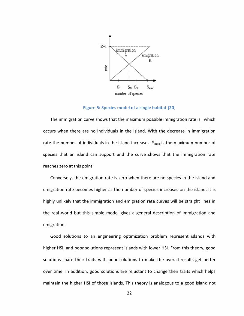
It can be seen from Figure 5 that immigration rate is zero when the number of
species is maximum, and immigration rate is maximum when the number of species is
zero. This shows that the immigration rate is zero (fewer new individuals coming in to
the island) and the emigration rate is maximum (more individuals going out of the
island) when HSI is high.
22
Figure 5: Species model of a single habitat [20]
The immigration curve shows that the maximum possible immigration rate is I which
occurs when there are no individuals in the island. With the decrease in immigration
rate the number of individuals in the island increases. Smax is the maximum number of
species that an island can support and the curve shows that the immigration rate
reaches zero at this point.
Conversely, the emigration rate is zero when there are no species in the island and
emigration rate becomes higher as the number of species increases on the island. It is
highly unlikely that the immigration and emigration rate curves will be straight lines in
the real world but this simple model gives a general description of immigration and
emigration.
Good solutions to an engineering optimization problem represent islands with
higher HSI, and poor solutions represent islands with lower HSI. From this theory, good
solutions share their traits with poor solutions to make the overall results get better
over time. In addition, good solutions are reluctant to change their traits which helps
maintain the higher HSI of those islands. This theory is analogous to a good island not
S0
23
receiving more species from the outside, but species from a better habitat will migrate
to a poor habitat. Poor solutions will benefit from this approach and the quality of the
habitat will eventually become better. This approach to problem solving is called
biogeography-based optimization (BBO).
BBO has some features in common with other biology based algorithms such as the
genetic algorithm (GA) and particle swarm optimization (PSO). The performance of BBO
compares well with other biology based algorithms as demonstrated in [20] on a set of
14 standard optimization benchmark functions. However, the focus of this thesis is to
apply biogeography-based optimization algorithm to robot navigation algorithms.
The curve of Figure 5 also shows two solutions, S1 and S2. S1 is a relatively poor
solution compared to S2. BBO can be applied to a problem where we have some
candidate solutions that are represented by vectors of real numbers. These numbers
will be called SIVs in BBO terminology. The solutions are then evaluated based on a
fitness scale and the habitats with better solutions have a high HSI and the poor
solutions are considered habitats with lower HSI. We consider that habitats with higher
HSI have more species and the habitats with lower HSI have comparatively fewer
species. The immigration and emigration curves shown in Figure 5 are considered to be
identical for all habitats (that is, all candidate solutions).
Immigration and emigration rates are used to probabilistically share information
between habitats. When a given solution is selected to be modified, immigration rate is
checked to determine whether an SIV will be modified in that solution. When a given SIV
is selected to be modified in a given solution Si, emigration rate is used to determine
24
which of the other solutions will be used to migrate or replace a selected SIV in solution
Si.
BBO also uses elitism to replace our worst two solutions with the best two from the
previous generation, or iteration. This makes sure that we never lose the best solutions
from one generation to the next.
BBO has been successfully applied to various problems. BBO was used to develop
open loop control for a semi-active hydraulic prosthetic knee [22]. The research
demonstrates that BBO is successful at finding optimal solutions of complex control
problems based on mathematical models. Distributed biogeography-based optimization
(DBBO) is an extension of the BBO which demonstrates that BBO can be successfully
used to optimize the low-level control algorithms of mobile robots [21].
For our purposes, BBO is used to optimize the bias, window angle and direction
strategy, which are described in following chapter. We used a 10 element vector to
parameterize a PRM algorithm, with the first element being the bias, the second
element being the window angle and the remaining eight elements being the direction
strategy FSM described in the following chapter. BBO was run with different
configurations to find the optimal generation size, population size, and mutation
probability, as described in Chapter VI. After optimizing the PRM parameters using BBO
we implement our results using PRM and demonstrate it using the robot.
25
CHAPTER IV
IMPLEMENTATION OF PATH PLANNING ALGORITHM
This chapter will focus on the implementation of the path planning simulation,
which includes localization of the robot, defining the robot work-space, defining the
obstacles, and checking for robot collisions with the obstacles. Section 4.1 discusses the
path planning algorithm, Section 4.2 introduces the obstacles, and Section 4.3 illustrates
the generation of the initial and goal points. Section 4.4 covers the main PRM
algorithm, including finding the next vertex (Section 4.4.1), obstacle-checking for the
path (Section 4.4.2), and obstacle checking for the current and next vertex
(Section 4.4.3). The commands sent from MATLAB to the robot controller are covered in
Section 4.5.
4.1 Path Planning Algorithm
The Monte Carlo simulation function serves as the stand-alone interactive testing
routine for PRM. PRM includes the following parameters: window angle, bias and
26
direction strategy. Biogeography-based optimization (BBO) has been used to tune these
parameters.
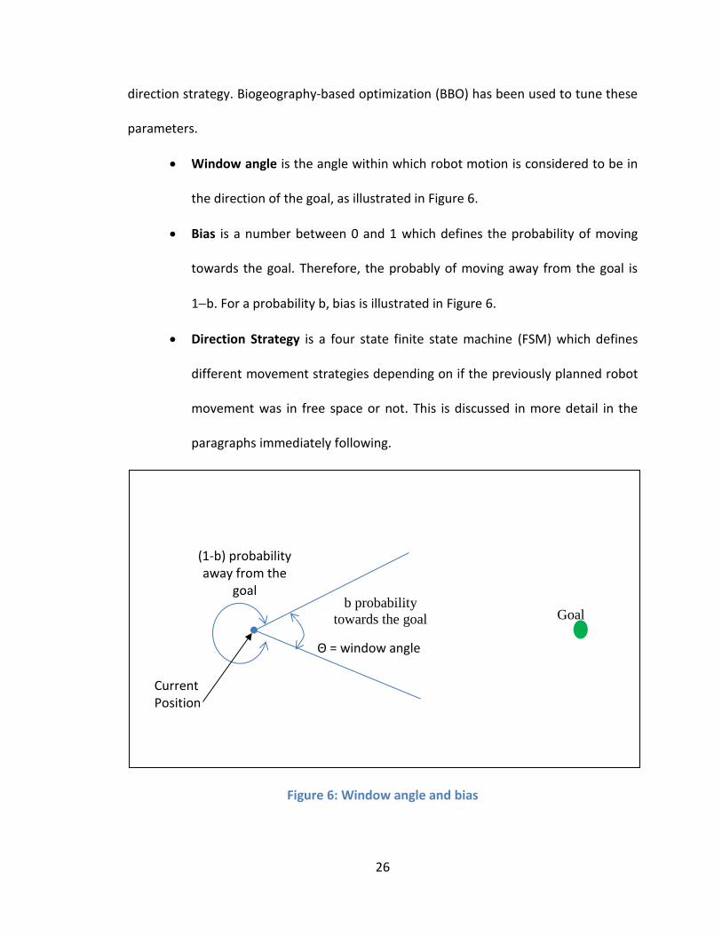
Window angle is the angle within which robot motion is considered to be in
the direction of the goal, as illustrated in Figure 6.
Bias is a number between 0 and 1 which defines the probability of moving
towards the goal. Therefore, the probably of moving away from the goal is
1b. For a probability b, bias is illustrated in Figure 6.
Direction Strategy is a four state finite state machine (FSM) which defines
different movement strategies depending on if the previously planned robot
movement was in free space or not. This is discussed in more detail in the
paragraphs immediately following.
Figure 6: Window angle and bias
Θ = window angle
Goal
Current Position
(1-b) probability away from the
goal b probability
towards the goal
27
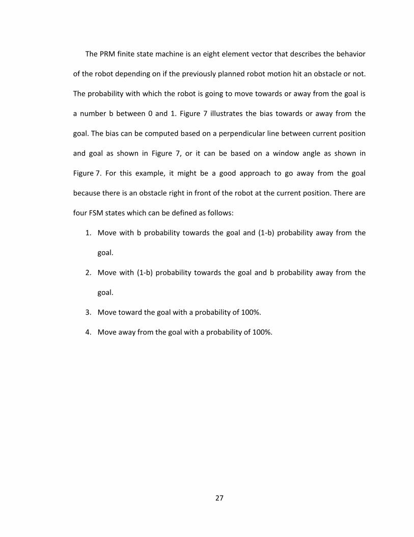
The PRM finite state machine is an eight element vector that describes the behavior
of the robot depending on if the previously planned robot motion hit an obstacle or not.
The probability with which the robot is going to move towards or away from the goal is
a number b between 0 and 1. Figure 7 illustrates the bias towards or away from the
goal. The bias can be computed based on a perpendicular line between current position
and goal as shown in Figure 7, or it can be based on a window angle as shown in
Figure 7. For this example, it might be a good approach to go away from the goal
because there is an obstacle right in front of the robot at the current position. There are
four FSM states which can be defined as follows:
1. Move with b probability towards the goal and (1-b) probability away from the
goal.
2. Move with (1-b) probability towards the goal and b probability away from the
goal.
3. Move toward the goal with a probability of 100%.
4. Move away from the goal with a probability of 100%.
28
Figure 7: Bias towards or away from the goal
The FSM is an eight element vector that includes the four states mentioned above in
case the previously planned robot motion was in free space or not. Each element of the
FSM vector is shown in Table 1. S represents the state of the FSM and F or H represents
if the previously planned robot motion was in free space or hit an obstacle. S(i, F)
indicates the state to which the robot will transition in case the robot is currently in
state i and is moving to a free space. Similarly, S(i, H) indicates the state to which the
robot will transition in case the robot is currently in state i and tried to move to a point
that was blocked by an obstacle.
S(1, F) S(1, H) S(2, F) S(2, H) S(3, F) S(3, H) S(4, F) S(4, H)
Table 1: Eight element vector of FSM
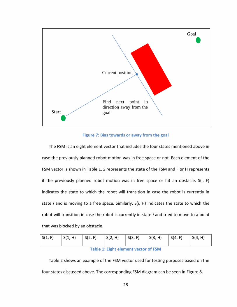
Table 2 shows an example of the FSM vector used for testing purposes based on the
four states discussed above. The corresponding FSM diagram can be seen in Figure 8.
Start
Goal
Current position
Find next point in
direction away from the
goal
29
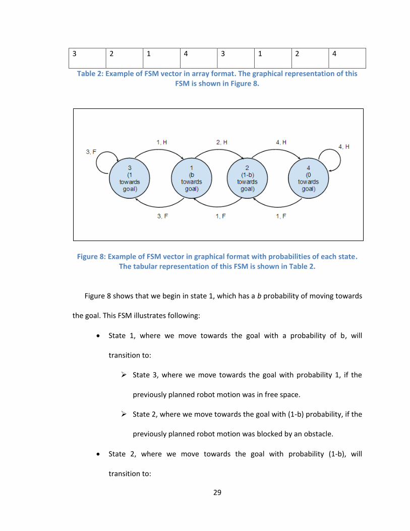
3 2 1 4 3 1 2 4
Table 2: Example of FSM vector in array format. The graphical representation of this FSM is shown in Figure 8.
Figure 8: Example of FSM vector in graphical format with probabilities of each state. The tabular representation of this FSM is shown in Table 2.
Figure 8 shows that we begin in state 1, which has a b probability of moving towards
the goal. This FSM illustrates following:
State 1, where we move towards the goal with a probability of b, will
transition to:
State 3, where we move towards the goal with probability 1, if the
previously planned robot motion was in free space.
State 2, where we move towards the goal with (1-b) probability, if the
previously planned robot motion was blocked by an obstacle.
State 2, where we move towards the goal with probability (1-b), will
transition to:
30
State 1, where we move towards the goal with b probability, if the
previously planned robot motion was in free space.
State 4, where we move away from the goal with probability 1, if the
previously planned robot motion was blocked by an obstacle.
State 3, where we move towards the goal with probability 1, will transition
to:
State 3, where we move towards the goal with probability 1, if the
previously planned robot motion was in free space.
State 1, where we move towards the goal with probability b, if the
previously planned robot motion was blocked by an obstacle.
State 4, where we move towards the goal with probability 0, will transition
to:
State 2, where we move towards the goal with probability (1-b), if the
previously planned robot motion was in free space.
State 4, where we move towards the goal with probability 0, if the
previously planned robot motion was blocked by an obstacle.
The output of the Monte Carlo simulation function is the mean of following results
(see Section 1.1) over a user-specified number of simulations:
Length of the path the robot takes to reach the goal from the start position.
Total number of hops is the number of straight-line segments that the robot
takes to reach its goal from the start position.
31
Total number of main-loop calls gives us the computational resources
utilized to find the path between the start and the goal.
Fail-rate is the percentage of PRM evaluations (over a given number of
Monte Carlo simulations) that fail to find a path to the goal within N main
loop calls, where N is a user-specified limit.
4.2 Obstacles
The “define obstacles” function will construct the random or pre-defined obstacles
for the robot world. The inputs to this function will be the number of obstacles required
for the test, the number of vertices in each obstacle, a randomness test flag, and size of
the robot world. The output of this function will be a cell array of row size one and
column size equal to the number of obstacles. Each cell in the obstacle cell array
contains the dimensions of one obstacle.
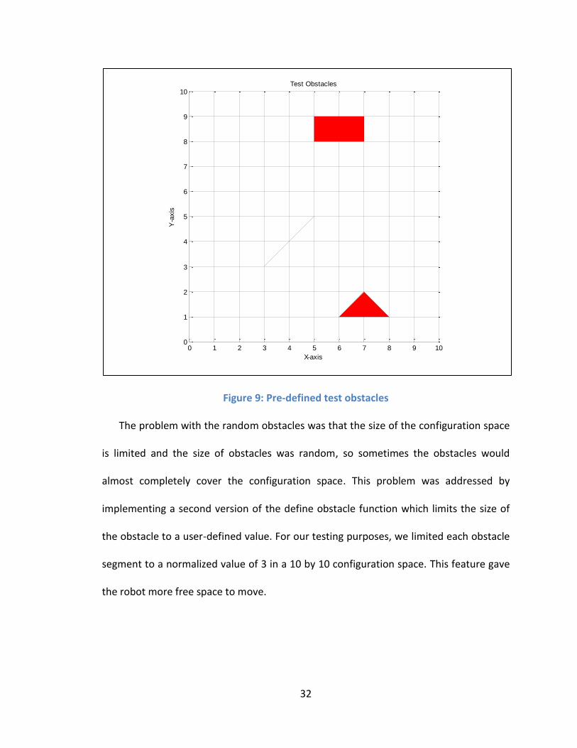
The pre-defined obstacles are used for testing and debugging purposes. The pre-
defined obstacles used for testing are a line segment, a triangle and a rectangle. Figure
9 shows the pre-defined test obstacles used for testing and debugging. We create
random obstacles in the configuration space when the randomness test flag is set.
Currently, random obstacle functionality is tested with 2 (line segment) or 3 (triangle)
point obstacles but it can be further extended to obstacles with more points with some
modification in the code.
32
Figure 9: Pre-defined test obstacles
The problem with the random obstacles was that the size of the configuration space
is limited and the size of obstacles was random, so sometimes the obstacles would
almost completely cover the configuration space. This problem was addressed by
implementing a second version of the define obstacle function which limits the size of
the obstacle to a user-defined value. For our testing purposes, we limited each obstacle
segment to a normalized value of 3 in a 10 by 10 configuration space. This feature gave
the robot more free space to move.
0 1 2 3 4 5 6 7 8 9 100
1
2
3
4
5
6
7
8
9
10
X-axis
Y-a
xis
Test Obstacles
33
4.3 Initial and Goal Points
The “get initial and goal” function will define the initial and goal locations. The
inputs to this function are a randomness flag, the number of obstacles, the radius of the
circle enclosing the robot, the robot world size, and the obstacle cell array. The output
of this function will be the X and Y coordinates of the initial and goal locations.
For the random test, this function calls two functions if the obstacles are triangles to
check if the initial or goal point is on the edges of the obstacle, or if the initial or goal
point lies inside the obstacle. If either case is true, the function gets new random initial
and goal points and starts checking the first obstacle. This loop breaks out if all the
obstacles have been checked and none of the points are inside or on the edges of any
obstacle.
A second version of this function was implemented to improve the performance of
this function. In the first version, we are finding a set of points (start and goal) which do
not lie inside any obstacle or intersect any obstacle. We were discarding the points if
either the start or goal point was not good. In the second version, we find the start and
goal separately. This allowed us to get the initial and goal points much faster than the
first version.
The problem with the first and second functions was that sometimes they would
find the start and goal very close to each other. This led us to write a third version which
takes a threshold value as an input. This threshold determines the minimum distance
between the start and goal positions.
34
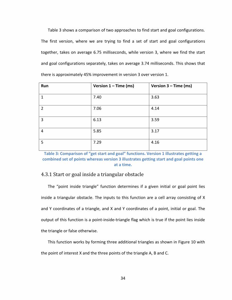
Table 3 shows a comparison of two approaches to find start and goal configurations.
The first version, where we are trying to find a set of start and goal configurations
together, takes on average 6.75 milliseconds, while version 3, where we find the start
and goal configurations separately, takes on average 3.74 milliseconds. This shows that
there is approximately 45% improvement in version 3 over version 1.
Run Version 1 – Time (ms) Version 3 – Time (ms)
1 7.40 3.63
2 7.06 4.14
3 6.13 3.59
4 5.85 3.17
5 7.29 4.16
Table 3: Comparison of “get start and goal” functions. Version 1 illustrates getting a combined set of points whereas version 3 illustrates getting start and goal points one
at a time.
4.3.1 Start or goal inside a triangular obstacle
The “point inside triangle” function determines if a given initial or goal point lies
inside a triangular obstacle. The inputs to this function are a cell array consisting of X
and Y coordinates of a triangle, and X and Y coordinates of a point, initial or goal. The
output of this function is a point-inside-triangle flag which is true if the point lies inside
the triangle or false otherwise.
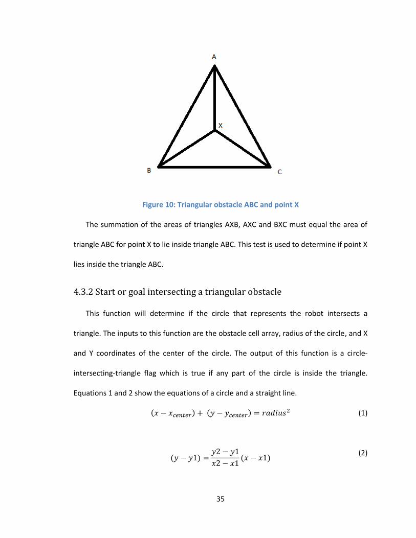
This function works by forming three additional triangles as shown in Figure 10 with
the point of interest X and the three points of the triangle A, B and C.
35
Figure 10: Triangular obstacle ABC and point X
The summation of the areas of triangles AXB, AXC and BXC must equal the area of
triangle ABC for point X to lie inside triangle ABC. This test is used to determine if point X
lies inside the triangle ABC.
4.3.2 Start or goal intersecting a triangular obstacle
This function will determine if the circle that represents the robot intersects a
triangle. The inputs to this function are the obstacle cell array, radius of the circle, and X
and Y coordinates of the center of the circle. The output of this function is a circle-
intersecting-triangle flag which is true if any part of the circle is inside the triangle.
Equations 1 and 2 show the equations of a circle and a straight line.
( ) ( ) (1)
( )
( )
(2)
36
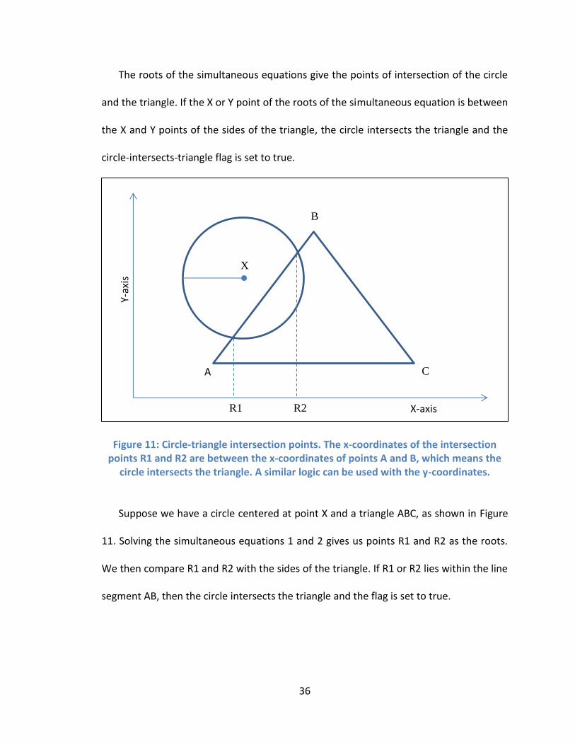
The roots of the simultaneous equations give the points of intersection of the circle
and the triangle. If the X or Y point of the roots of the simultaneous equation is between
the X and Y points of the sides of the triangle, the circle intersects the triangle and the
circle-intersects-triangle flag is set to true.
Figure 11: Circle-triangle intersection points. The x-coordinates of the intersection points R1 and R2 are between the x-coordinates of points A and B, which means the
circle intersects the triangle. A similar logic can be used with the y-coordinates.
Suppose we have a circle centered at point X and a triangle ABC, as shown in Figure
11. Solving the simultaneous equations 1 and 2 gives us points R1 and R2 as the roots.
We then compare R1 and R2 with the sides of the triangle. If R1 or R2 lies within the line
segment AB, then the circle intersects the triangle and the flag is set to true.
X-axis
Y-ax
is
A
B
C
R1 R2
X
37
4.4 Probabilistic Roadmaps Method
This function implements the idea presented in [2]. The inputs to this function are
bias, window angle and default bias. The outputs of this function are vertex-edge array,
path length, number of hops, number of loops and fail-rate. This function is also
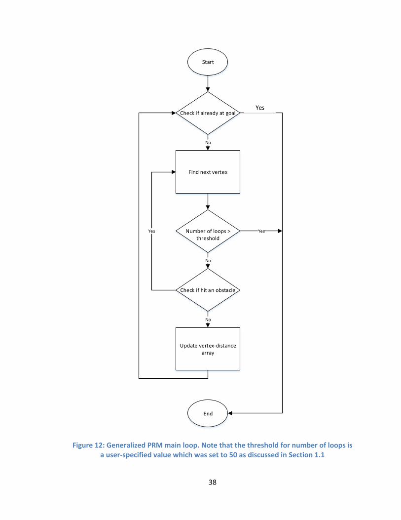
responsible for the plotting features. The main loop of this function is shown in Figure
12. We start by checking if we are already at the goal. We then find the next potential
vertex to move the robot to the next position. We then check if the node we found, and
the path to that node, is in free space. If it is in free space we update the vertex-edge
array and repeat the main loop. If it is not in free space we ignore the next vertex and
do not update the vertex-edge array, and instead find another vertex.
38
Find next vertex
Update vertex-distance array
Check if already at goal
Check if hit an obstacle
No
No
Yes Number of loops > threshold
No
Start
End
Yes
Yes
Figure 12: Generalized PRM main loop. Note that the threshold for number of loops is a user-specified value which was set to 50 as discussed in Section 1.1
39
We used the bias, window angle, locations and the direction strategy to find the
next vertex. The implementation of this modified function can be shown as follows:
1. Check to see if the robot is already at the goal.
2. Find the next vertex based on the direction strategy, bias and window angle.
3. Check if the next vertex, or the path to that vertex, intersects an obstacle.
4. Update the next vertex distance array if the vertex and the path are in free
space; otherwise go to step 2.
5. Find the next state based on the previous state.
6. Extract the new bias from the new state.
4.4.1 Finding the next vertex
This function implements the algorithm to find the next vertex depending on the
current position. The inputs to this function are current position, goal position, bias,
window angle and radius of the robot. The outputs of this function are the X and Y
coordinates of the next position. Three different approaches were used to calculate the
coordinates of the next position.
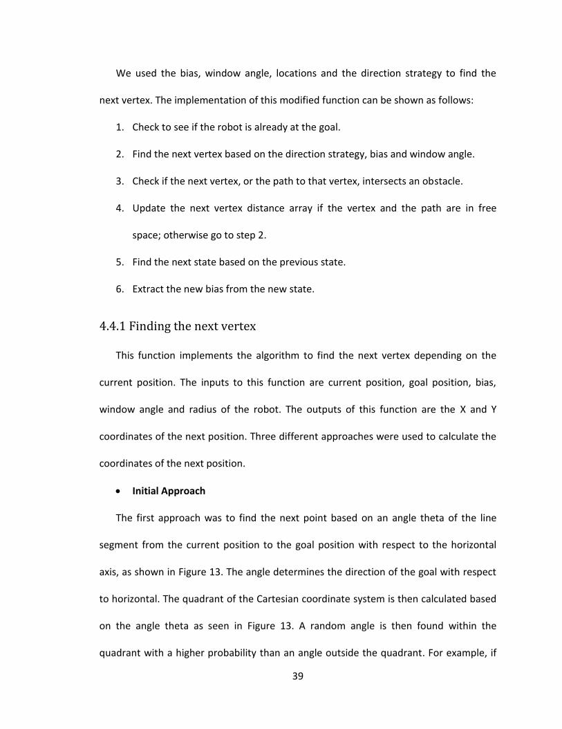
Initial Approach
The first approach was to find the next point based on an angle theta of the line
segment from the current position to the goal position with respect to the horizontal
axis, as shown in Figure 13. The angle determines the direction of the goal with respect
to horizontal. The quadrant of the Cartesian coordinate system is then calculated based
on the angle theta as seen in Figure 13. A random angle is then found within the
quadrant with a higher probability than an angle outside the quadrant. For example, if
40
the goal lies in quadrant I then a random angle between 0o and 90o is found, with
probability b. On the other hand, a random angle between 90o and 360o is found, with
probability (1-b).
Figure 13: Next vertex based on horizontal axis
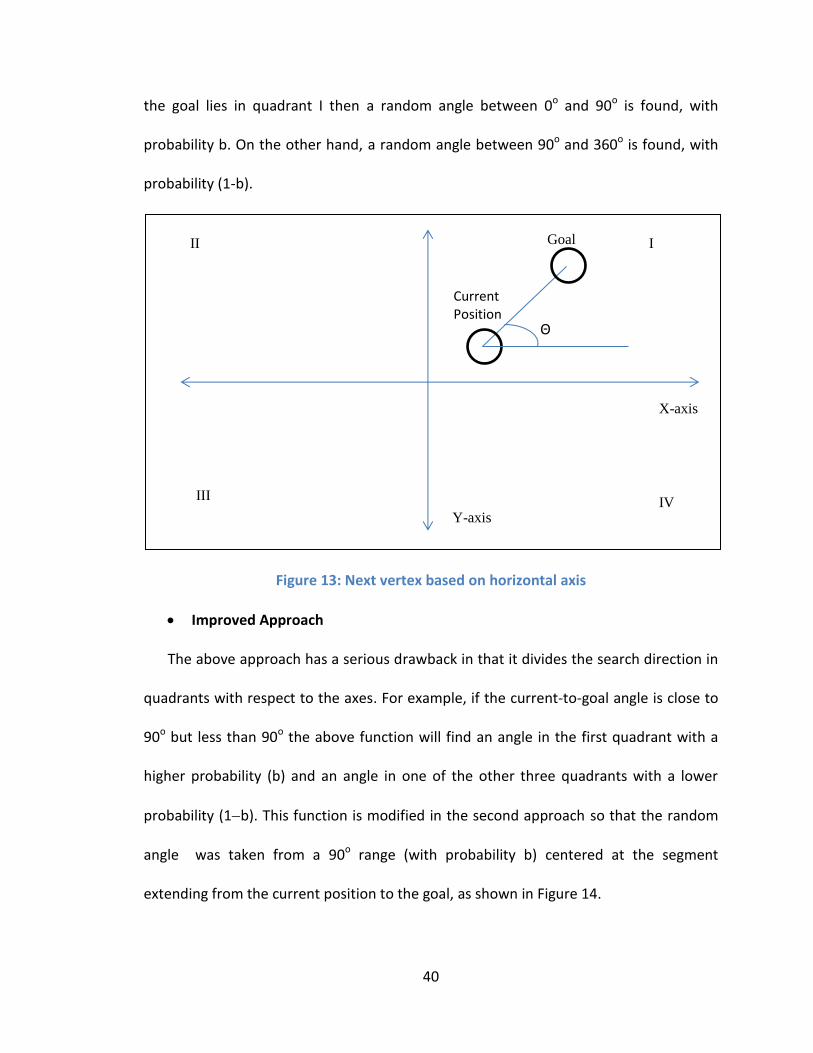
Improved Approach
The above approach has a serious drawback in that it divides the search direction in
quadrants with respect to the axes. For example, if the current-to-goal angle is close to
90o but less than 90o the above function will find an angle in the first quadrant with a
higher probability (b) and an angle in one of the other three quadrants with a lower
probability (1b). This function is modified in the second approach so that the random
angle was taken from a 90o range (with probability b) centered at the segment
extending from the current position to the goal, as shown in Figure 14.
Current Position
Goal
Y-axis
X-axis
Θ
I
IV
II
III
41
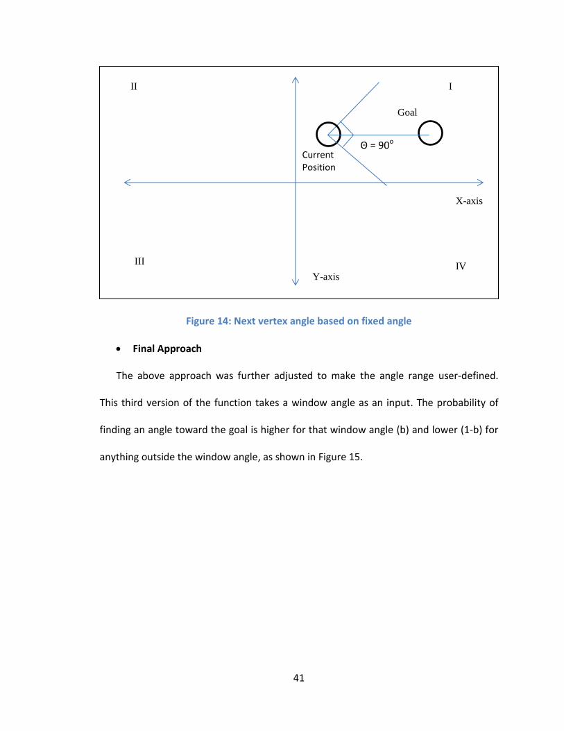
Figure 14: Next vertex angle based on fixed angle
Final Approach
The above approach was further adjusted to make the angle range user-defined.
This third version of the function takes a window angle as an input. The probability of
finding an angle toward the goal is higher for that window angle (b) and lower (1-b) for
anything outside the window angle, as shown in Figure 15.
Current Position
Goal
Y-axis
X-axis
Θ = 90o
I
IV
II
III
42
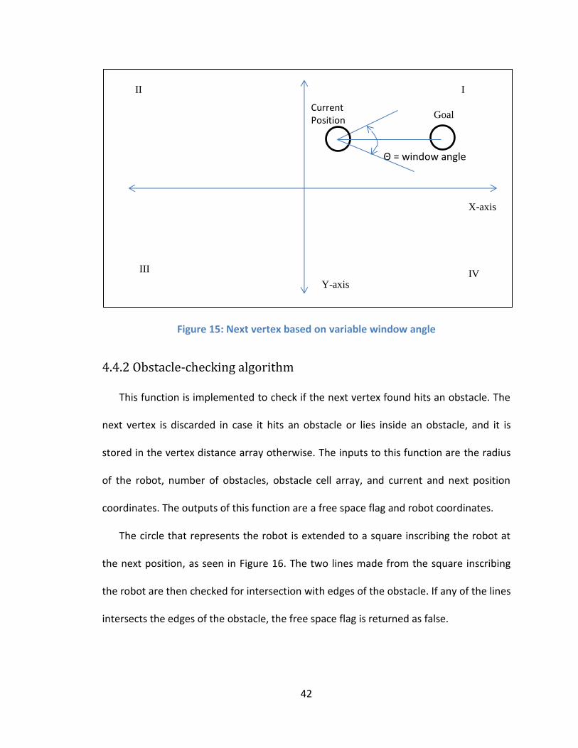
Figure 15: Next vertex based on variable window angle
4.4.2 Obstacle-checking algorithm
This function is implemented to check if the next vertex found hits an obstacle. The
next vertex is discarded in case it hits an obstacle or lies inside an obstacle, and it is
stored in the vertex distance array otherwise. The inputs to this function are the radius
of the robot, number of obstacles, obstacle cell array, and current and next position
coordinates. The outputs of this function are a free space flag and robot coordinates.
The circle that represents the robot is extended to a square inscribing the robot at
the next position, as seen in Figure 16. The two lines made from the square inscribing
the robot are then checked for intersection with edges of the obstacle. If any of the lines
intersects the edges of the obstacle, the free space flag is returned as false.
Current Position
Goal
Y-axis
X-axis
Θ = window angle
I
IV
II
III
43
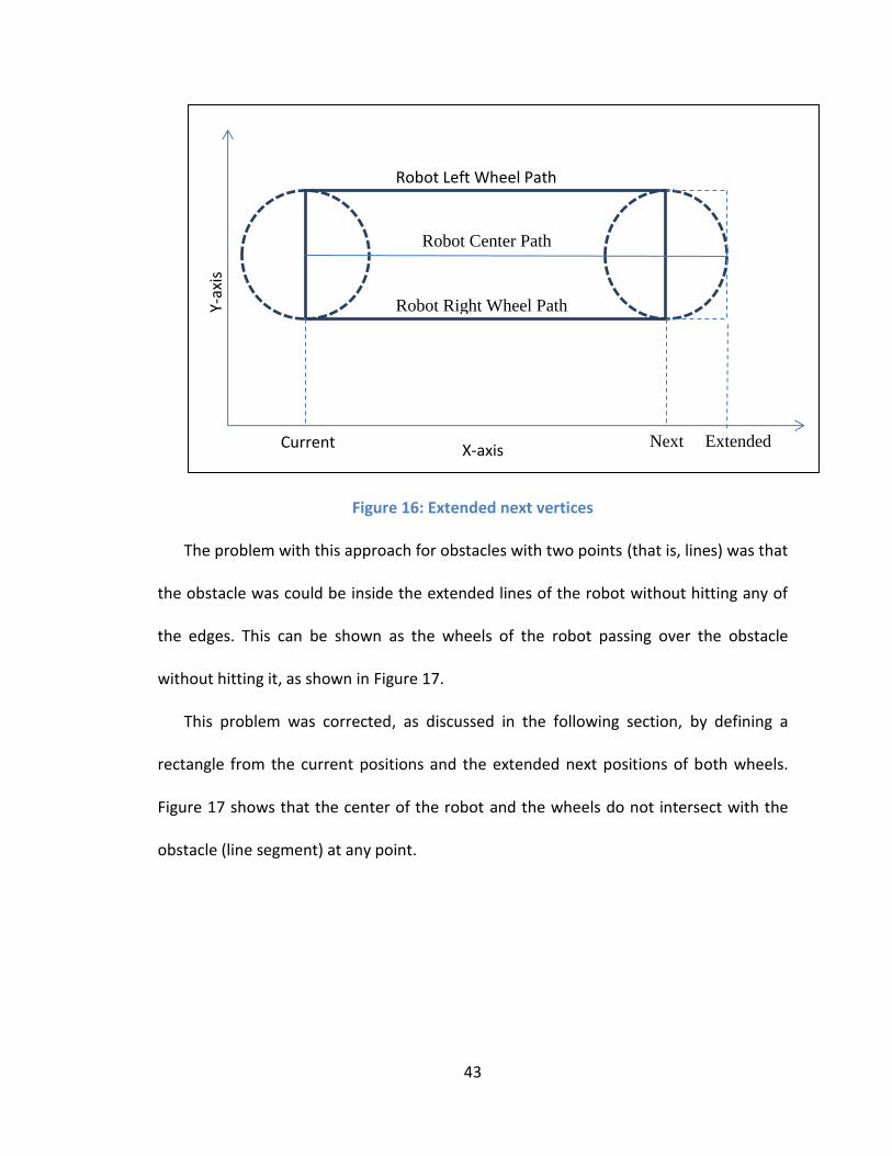
Figure 16: Extended next vertices
The problem with this approach for obstacles with two points (that is, lines) was that
the obstacle was could be inside the extended lines of the robot without hitting any of
the edges. This can be shown as the wheels of the robot passing over the obstacle
without hitting it, as shown in Figure 17.
This problem was corrected, as discussed in the following section, by defining a
rectangle from the current positions and the extended next positions of both wheels.
Figure 17 shows that the center of the robot and the wheels do not intersect with the
obstacle (line segment) at any point.
Robot Left Wheel Path
Robot Right Wheel Path
Robot Center Path
X-axis
Y-ax
is
Current Next Extended
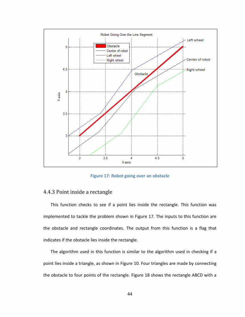
44
Figure 17: Robot going over an obstacle
4.4.3 Point inside a rectangle
This function checks to see if a point lies inside the rectangle. This function was
implemented to tackle the problem shown in Figure 17. The inputs to this function are
the obstacle and rectangle coordinates. The output from this function is a flag that
indicates if the obstacle lies inside the rectangle.
The algorithm used in this function is similar to the algorithm used in checking if a
point lies inside a triangle, as shown in Figure 10. Four triangles are made by connecting
the obstacle to four points of the rectangle. Figure 18 shows the rectangle ABCD with a
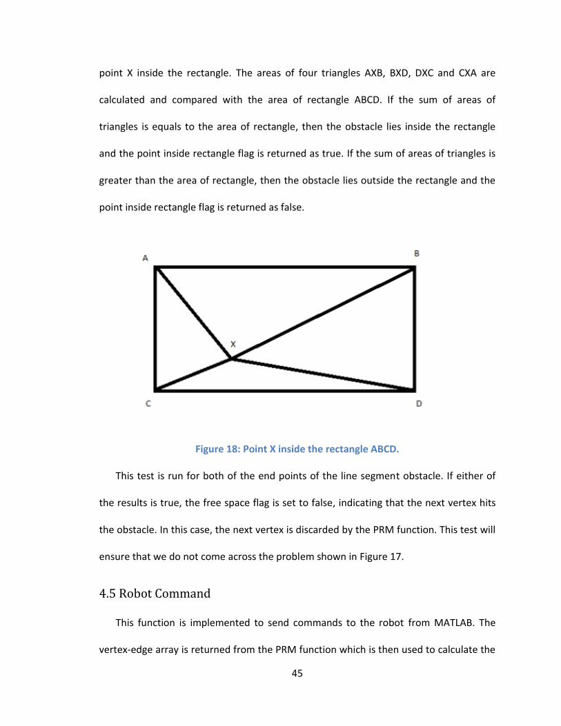
45
point X inside the rectangle. The areas of four triangles AXB, BXD, DXC and CXA are
calculated and compared with the area of rectangle ABCD. If the sum of areas of
triangles is equals to the area of rectangle, then the obstacle lies inside the rectangle
and the point inside rectangle flag is returned as true. If the sum of areas of triangles is
greater than the area of rectangle, then the obstacle lies outside the rectangle and the
point inside rectangle flag is returned as false.
Figure 18: Point X inside the rectangle ABCD.
This test is run for both of the end points of the line segment obstacle. If either of
the results is true, the free space flag is set to false, indicating that the next vertex hits
the obstacle. In this case, the next vertex is discarded by the PRM function. This test will
ensure that we do not come across the problem shown in Figure 17.
4.5 Robot Command
This function is implemented to send commands to the robot from MATLAB. The
vertex-edge array is returned from the PRM function which is then used to calculate the

46
straight-line distance in meters and the angle of rotation in degrees. This function then
opens a serial connection to the specified port and sends the command to the radio.
The command is sent as a 16-bit integer which is followed by a user prompt to press any
key which then sends the next command. The command is sent in the format of rotation
followed by distance for each hop until the goal is reached. Section 6.2 gives an example
of the commands sent from the MATLAB and how they are received by the robot
hardware to perform the desired operation.
47
CHAPTER V
HARDWARE AND EMBEDDED IMPLEMENTATION
This chapter will cover the embedded implementation of the robots. This chapter
describes the testing and implementation of simulations done in MATLAB. We will also
discuss the hardware used and the communication between various components.
Section 5.1 discusses the hardware implementation for this thesis. Section 5.2 discusses
the Microchip peripheral interface controller which serves as the brains of the robot.
Section 5.3 describes the software implementation and interface of programming the
robot hardware.
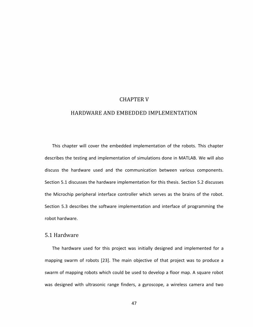
5.1 Hardware
The hardware used for this project was initially designed and implemented for a
mapping swarm of robots [23]. The main objective of that project was to produce a
swarm of mapping robots which could be used to develop a floor map. A square robot
was designed with ultrasonic range finders, a gyroscope, a wireless camera and two

48
wheel encoders. The main circuitry is mounted on a printed circuit board with a
Microchip PIC18F4520 microcontroller, which provides the brains of the robot. The
robot also has an LCD, which is used for debugging and displaying real time messages.
The PCB layout shown in Figure 19 is used in the robot.
Figure 19: Printed circuit board used in robot [24]
Communication between the robot and the base station (that is, the personal
computer) is accomplished using a MaxStream 9Xtend RF transmitter-receiver pair. This
device supports an indoor range of 900 meters and operates on a selectable output
power of either 1 mW or 1 W. This device is mounted on both the robot and the base
station. The MaxStream 9Xtend wireless radio is shown in Figure 20.

49
Figure 20: Photograph of MaxStream 9Xtend wireless radio [21]
The robot is equipped with two DC motors which are used to rotate the left and
right wheels. Nubotics Wheel Watcher 2 encoders are mounted on each wheel to
measure the distance traveled by the robot. The timers from the PIC are configured as
counters to keep track of encoder counts. There are 64 stripes on the wheel encoders.
The radius of the wheel is 3.50 cm which gives a circumference of 21.99 cm. The
conversion factor of the encoders is derived by dividing the circumference of the wheel
by the number of encoder counts in one rotation, which comes out to 0.34 cm per
encoder count. This conversion factor is then multiplied by the number of encoder
counts over a given period of time to calculate the distance traveled by the wheel. The
robot used for the testing purposes is shown in Figure 21.
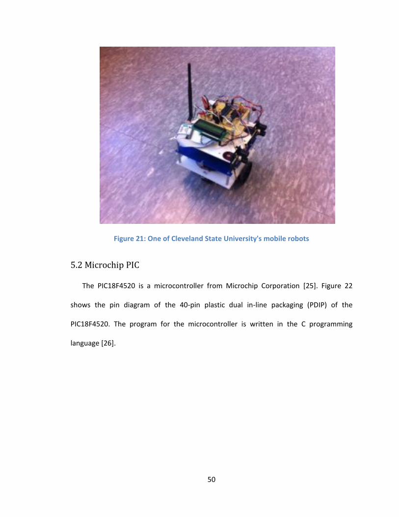
50
Figure 21: One of Cleveland State University's mobile robots
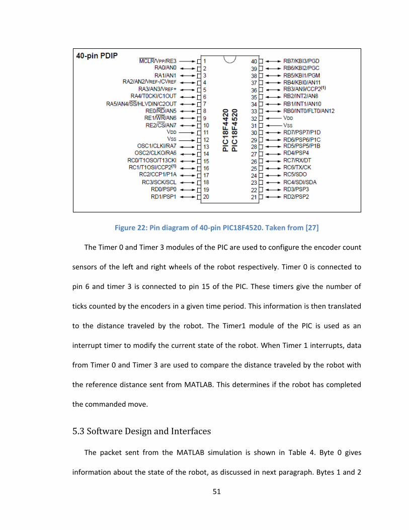
5.2 Microchip PIC
The PIC18F4520 is a microcontroller from Microchip Corporation [25]. Figure 22
shows the pin diagram of the 40-pin plastic dual in-line packaging (PDIP) of the
PIC18F4520. The program for the microcontroller is written in the C programming
language [26].
51
Figure 22: Pin diagram of 40-pin PIC18F4520. Taken from [27]
The Timer 0 and Timer 3 modules of the PIC are used to configure the encoder count
sensors of the left and right wheels of the robot respectively. Timer 0 is connected to
pin 6 and timer 3 is connected to pin 15 of the PIC. These timers give the number of
ticks counted by the encoders in a given time period. This information is then translated
to the distance traveled by the robot. The Timer1 module of the PIC is used as an
interrupt timer to modify the current state of the robot. When Timer 1 interrupts, data
from Timer 0 and Timer 3 are used to compare the distance traveled by the robot with
the reference distance sent from MATLAB. This determines if the robot has completed
the commanded move.
5.3 Software Design and Interfaces
The packet sent from the MATLAB simulation is shown in Table 4. Byte 0 gives
information about the state of the robot, as discussed in next paragraph. Bytes 1 and 2
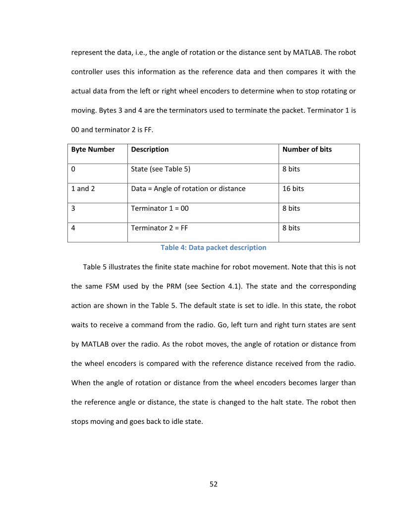
52
represent the data, i.e., the angle of rotation or the distance sent by MATLAB. The robot
controller uses this information as the reference data and then compares it with the
actual data from the left or right wheel encoders to determine when to stop rotating or
moving. Bytes 3 and 4 are the terminators used to terminate the packet. Terminator 1 is
00 and terminator 2 is FF.
Byte Number Description Number of bits
0 State (see Table 5) 8 bits
1 and 2 Data = Angle of rotation or distance 16 bits
3 Terminator 1 = 00 8 bits
4 Terminator 2 = FF 8 bits
Table 4: Data packet description
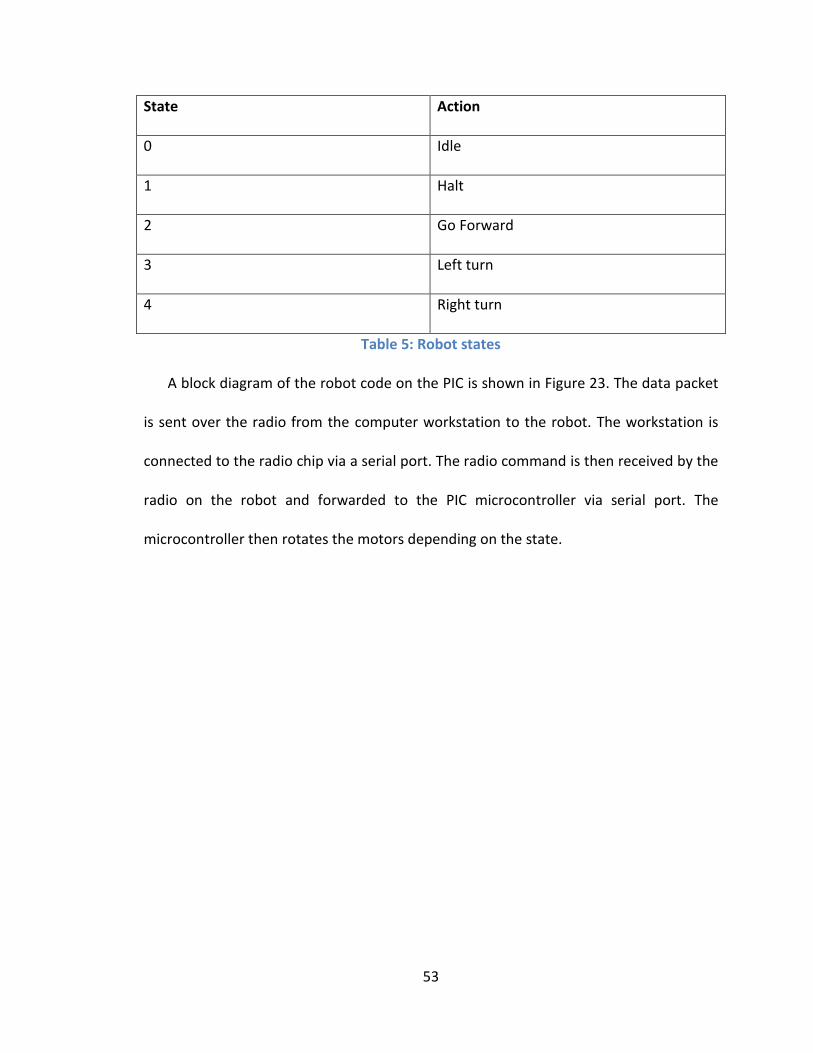
Table 5 illustrates the finite state machine for robot movement. Note that this is not
the same FSM used by the PRM (see Section 4.1). The state and the corresponding
action are shown in the Table 5. The default state is set to idle. In this state, the robot
waits to receive a command from the radio. Go, left turn and right turn states are sent
by MATLAB over the radio. As the robot moves, the angle of rotation or distance from
the wheel encoders is compared with the reference distance received from the radio.
When the angle of rotation or distance from the wheel encoders becomes larger than
the reference angle or distance, the state is changed to the halt state. The robot then
stops moving and goes back to idle state.
53
State Action
0 Idle
1 Halt
2 Go Forward
3 Left turn
4 Right turn
Table 5: Robot states
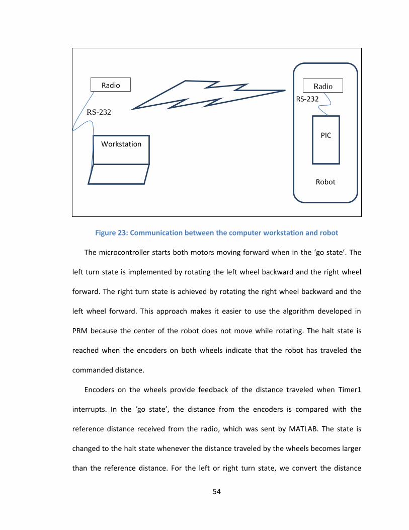
A block diagram of the robot code on the PIC is shown in Figure 23. The data packet
is sent over the radio from the computer workstation to the robot. The workstation is
connected to the radio chip via a serial port. The radio command is then received by the
radio on the robot and forwarded to the PIC microcontroller via serial port. The
microcontroller then rotates the motors depending on the state.
54
Figure 23: Communication between the computer workstation and robot
The microcontroller starts both motors moving forward when in the ‘go state’. The
left turn state is implemented by rotating the left wheel backward and the right wheel
forward. The right turn state is achieved by rotating the right wheel backward and the
left wheel forward. This approach makes it easier to use the algorithm developed in
PRM because the center of the robot does not move while rotating. The halt state is
reached when the encoders on both wheels indicate that the robot has traveled the
commanded distance.
Encoders on the wheels provide feedback of the distance traveled when Timer1
interrupts. In the ‘go state’, the distance from the encoders is compared with the
reference distance received from the radio, which was sent by MATLAB. The state is
changed to the halt state whenever the distance traveled by the wheels becomes larger
than the reference distance. For the left or right turn state, we convert the distance
Workstation
Radio
Robot
PIC
Radio
RS-232
RS-232
55
from the wheel encoders to an angle in radians and then compare it to the reference
angle received by the radio. The conversion of the wheel distance to the angle is given
as follows;
(3)
Here, theta is the angle rotated by the robot,
wheel1distance is the distance traveled by left wheel.
wheel2distance is the distance traveled by right wheel.
base_distance is the distance between the left and right wheel of the robot.
180/π is the factor to convert the angle from radians to degrees.
The derivation to find the angle of rotation is taken from [28] and is shown in Figure
24. Note that in Figure 24, wheel2distance is subtracted from wheel1distance, but we
take care of that by knowing whether we are in the left or right turn state.
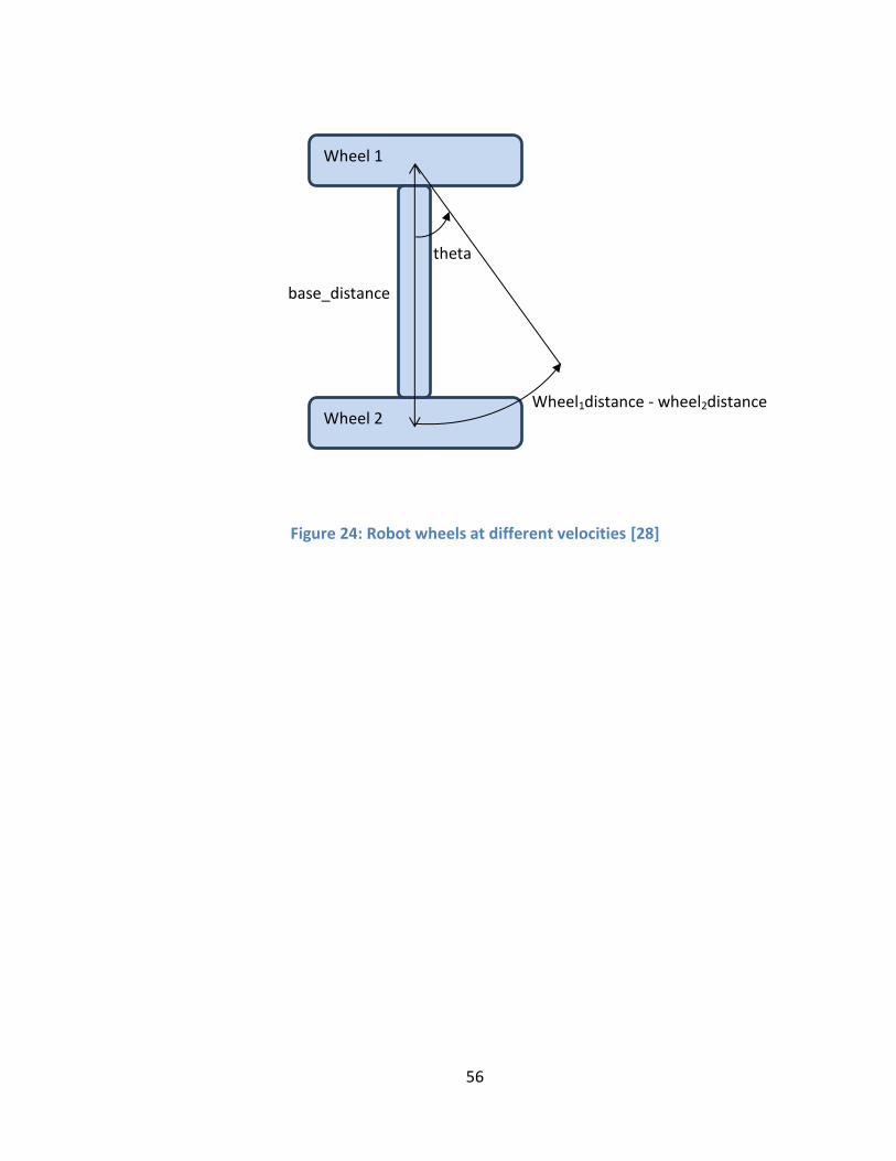
56
Figure 24: Robot wheels at different velocities [28]
Wheel 1
Wheel 2
theta
Wheel1distance - wheel2distance
base_distance
57
CHAPTER VI
RESULTS
This chapter will cover simulation and experimental results. Section 6.1 covers the
tuning of BBO parameters and using those BBO parameters to optimize PRM
parameters. Section 6.2 presents the experimental results where a mobile robot follows
the path found by PRM.
6.1 Simulation Results
6.1.1 BBO parameters
We begin by setting the default values for generation size, population size, mutation
probability and the number of individuals we want to keep for elitism in BBO. Table 6
shows the default values used in BBO.
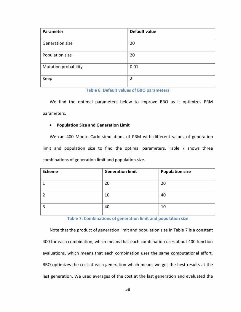
58
Parameter Default value
Generation size 20
Population size 20
Mutation probability 0.01
Keep 2
Table 6: Default values of BBO parameters
We find the optimal parameters below to improve BBO as it optimizes PRM
parameters.
Population Size and Generation Limit
We ran 400 Monte Carlo simulations of PRM with different values of generation
limit and population size to find the optimal parameters. Table 7 shows three
combinations of generation limit and population size.
Scheme Generation limit Population size
1 20 20
2 10 40
3 40 10
Table 7: Combinations of generation limit and population size
Note that the product of generation limit and population size in Table 7 is a constant
400 for each combination, which means that each combination uses about 400 function
evaluations, which means that each combination uses the same computational effort.
BBO optimizes the cost at each generation which means we get the best results at the
last generation. We used averages of the cost at the last generation and evaluated the
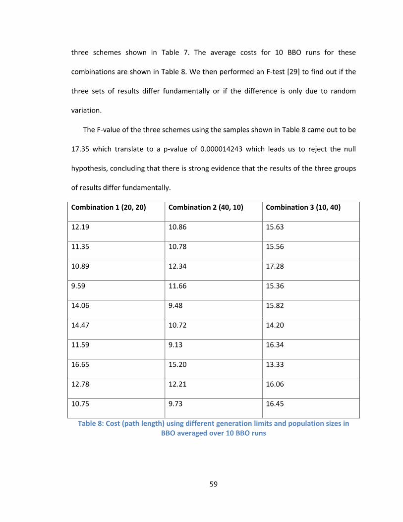
59
three schemes shown in Table 7. The average costs for 10 BBO runs for these
combinations are shown in Table 8. We then performed an F-test [29] to find out if the
three sets of results differ fundamentally or if the difference is only due to random
variation.
The F-value of the three schemes using the samples shown in Table 8 came out to be
17.35 which translate to a p-value of 0.000014243 which leads us to reject the null
hypothesis, concluding that there is strong evidence that the results of the three groups
of results differ fundamentally.
Combination 1 (20, 20) Combination 2 (40, 10) Combination 3 (10, 40)
12.19 10.86 15.63
11.35 10.78 15.56
10.89 12.34 17.28
9.59 11.66 15.36
14.06 9.48 15.82
14.47 10.72 14.20
11.59 9.13 16.34
16.65 15.20 13.33
12.78 12.21 16.06
10.75 9.73 16.45
Table 8: Cost (path length) using different generation limits and population sizes in BBO averaged over 10 BBO runs
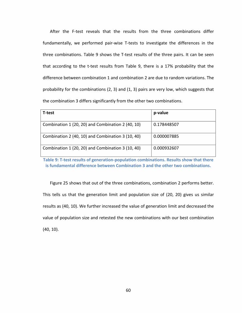
60
After the F-test reveals that the results from the three combinations differ
fundamentally, we performed pair-wise T-tests to investigate the differences in the
three combinations. Table 9 shows the T-test results of the three pairs. It can be seen
that according to the t-test results from Table 9, there is a 17% probability that the
difference between combination 1 and combination 2 are due to random variations. The
probability for the combinations (2, 3) and (1, 3) pairs are very low, which suggests that
the combination 3 differs significantly from the other two combinations.
T-test p-value
Combination 1 (20, 20) and Combination 2 (40, 10) 0.178448507
Combination 2 (40, 10) and Combination 3 (10, 40) 0.000007885
Combination 1 (20, 20) and Combination 3 (10, 40) 0.000932607
Table 9: T-test results of generation-population combinations. Results show that there is fundamental difference between Combination 3 and the other two combinations.
Figure 25 shows that out of the three combinations, combination 2 performs better.
This tells us that the generation limit and population size of (20, 20) gives us similar
results as (40, 10). We further increased the value of generation limit and decreased the
value of population size and retested the new combinations with our best combination
(40, 10).
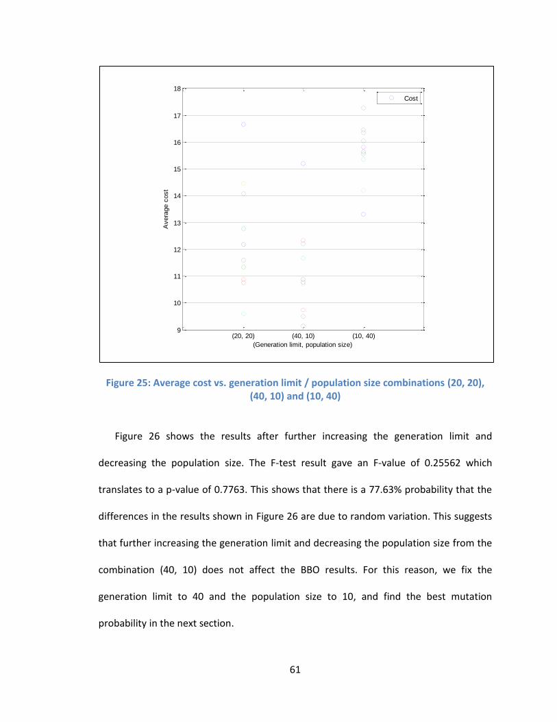
61
Figure 25: Average cost vs. generation limit / population size combinations (20, 20), (40, 10) and (10, 40)
Figure 26 shows the results after further increasing the generation limit and
decreasing the population size. The F-test result gave an F-value of 0.25562 which
translates to a p-value of 0.7763. This shows that there is a 77.63% probability that the
differences in the results shown in Figure 26 are due to random variation. This suggests
that further increasing the generation limit and decreasing the population size from the
combination (40, 10) does not affect the BBO results. For this reason, we fix the
generation limit to 40 and the population size to 10, and find the best mutation
probability in the next section.
(20, 20) (40, 10) (10, 40)9
10
11
12
13
14
15
16
17
18
(Generation limit, population size)
Avera
ge c
ost
Cost
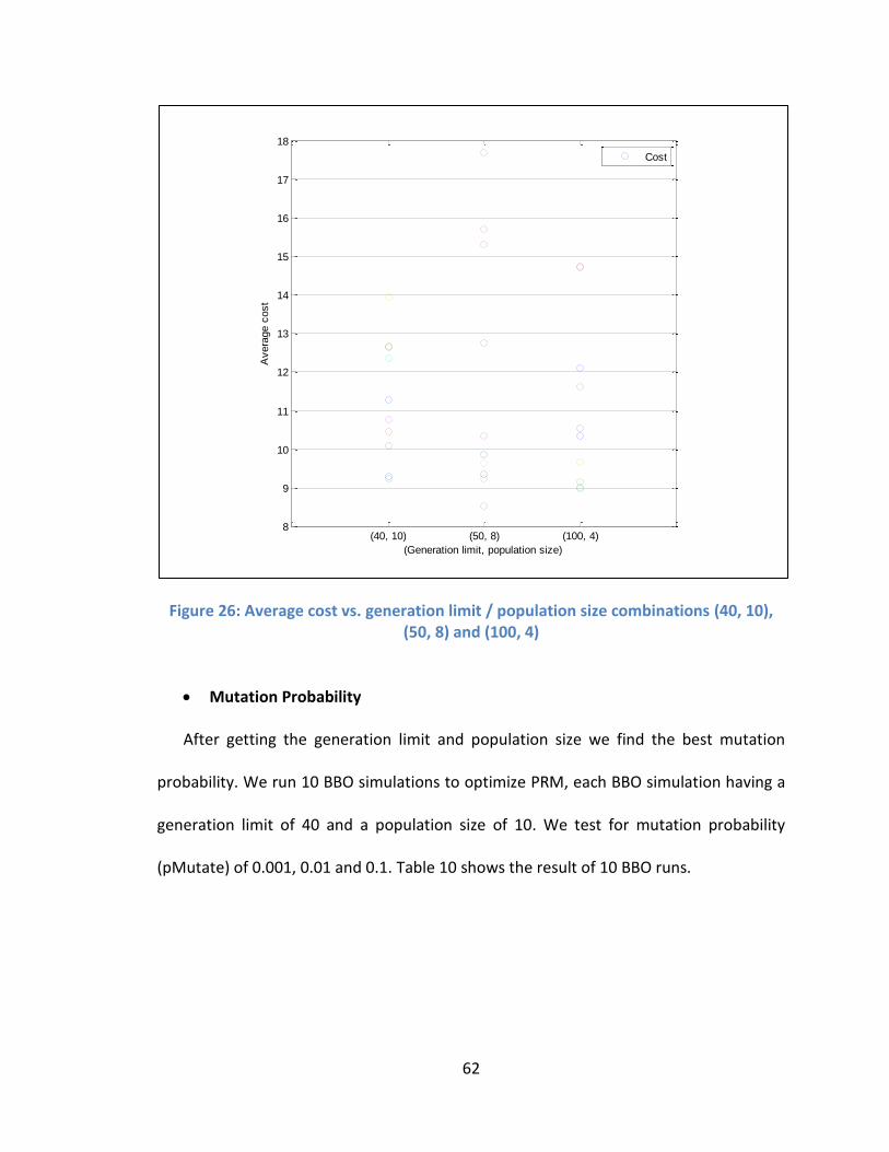
62
Figure 26: Average cost vs. generation limit / population size combinations (40, 10), (50, 8) and (100, 4)
Mutation Probability
After getting the generation limit and population size we find the best mutation
probability. We run 10 BBO simulations to optimize PRM, each BBO simulation having a
generation limit of 40 and a population size of 10. We test for mutation probability
(pMutate) of 0.001, 0.01 and 0.1. Table 10 shows the result of 10 BBO runs.
(40, 10) (50, 8) (100, 4)8
9
10
11
12
13
14
15
16
17
18
(Generation limit, population size)
Avera
ge c
ost
Cost
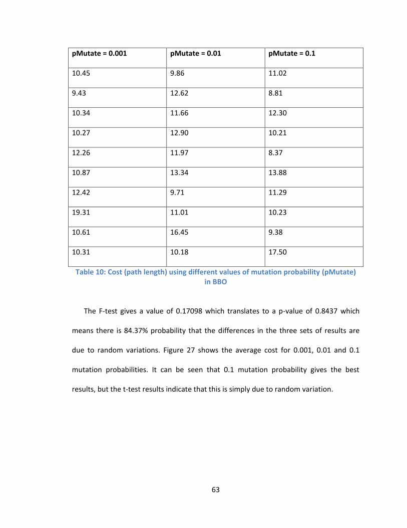
63
pMutate = 0.001 pMutate = 0.01 pMutate = 0.1
10.45 9.86 11.02
9.43 12.62 8.81
10.34 11.66 12.30
10.27 12.90 10.21
12.26 11.97 8.37
10.87 13.34 13.88
12.42 9.71 11.29
19.31 11.01 10.23
10.61 16.45 9.38
10.31 10.18 17.50
Table 10: Cost (path length) using different values of mutation probability (pMutate) in BBO
The F-test gives a value of 0.17098 which translates to a p-value of 0.8437 which
means there is 84.37% probability that the differences in the three sets of results are
due to random variations. Figure 27 shows the average cost for 0.001, 0.01 and 0.1
mutation probabilities. It can be seen that 0.1 mutation probability gives the best
results, but the t-test results indicate that this is simply due to random variation.
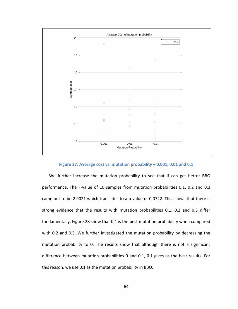
64
Figure 27: Average cost vs. mutation probability – 0.001, 0.01 and 0.1
We further increase the mutation probability to see that if can get better BBO
performance. The F-value of 10 samples from mutation probabilities 0.1, 0.2 and 0.3
came out to be 2.9021 which translates to a p-value of 0.0722. This shows that there is
strong evidence that the results with mutation probabilities 0.1, 0.2 and 0.3 differ
fundamentally. Figure 28 show that 0.1 is the best mutation probability when compared
with 0.2 and 0.3. We further investigated the mutation probability by decreasing the
mutation probability to 0. The results show that although there is not a significant
difference between mutation probabilities 0 and 0.1, 0.1 gives us the best results. For
this reason, we use 0.1 as the mutation probability in BBO.
0.001 0.01 0.18
10
12
14
16
18
20
Mutation Probability
Avera
ge c
ost
Average Cost of mutation probability
Cost
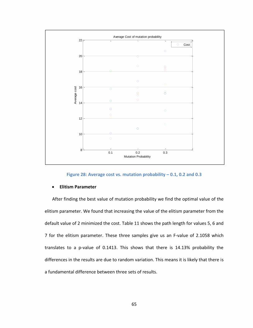
65
Figure 28: Average cost vs. mutation probability – 0.1, 0.2 and 0.3
Elitism Parameter
After finding the best value of mutation probability we find the optimal value of the
elitism parameter. We found that increasing the value of the elitism parameter from the
default value of 2 minimized the cost. Table 11 shows the path length for values 5, 6 and
7 for the elitism parameter. These three samples give us an F-value of 2.1058 which
translates to a p-value of 0.1413. This shows that there is 14.13% probability the
differences in the results are due to random variation. This means it is likely that there is
a fundamental difference between three sets of results.
0.1 0.2 0.38
10
12
14
16
18
20
22
Mutation Probability
Avera
ge c
ost
Average Cost of mutation probability
Cost
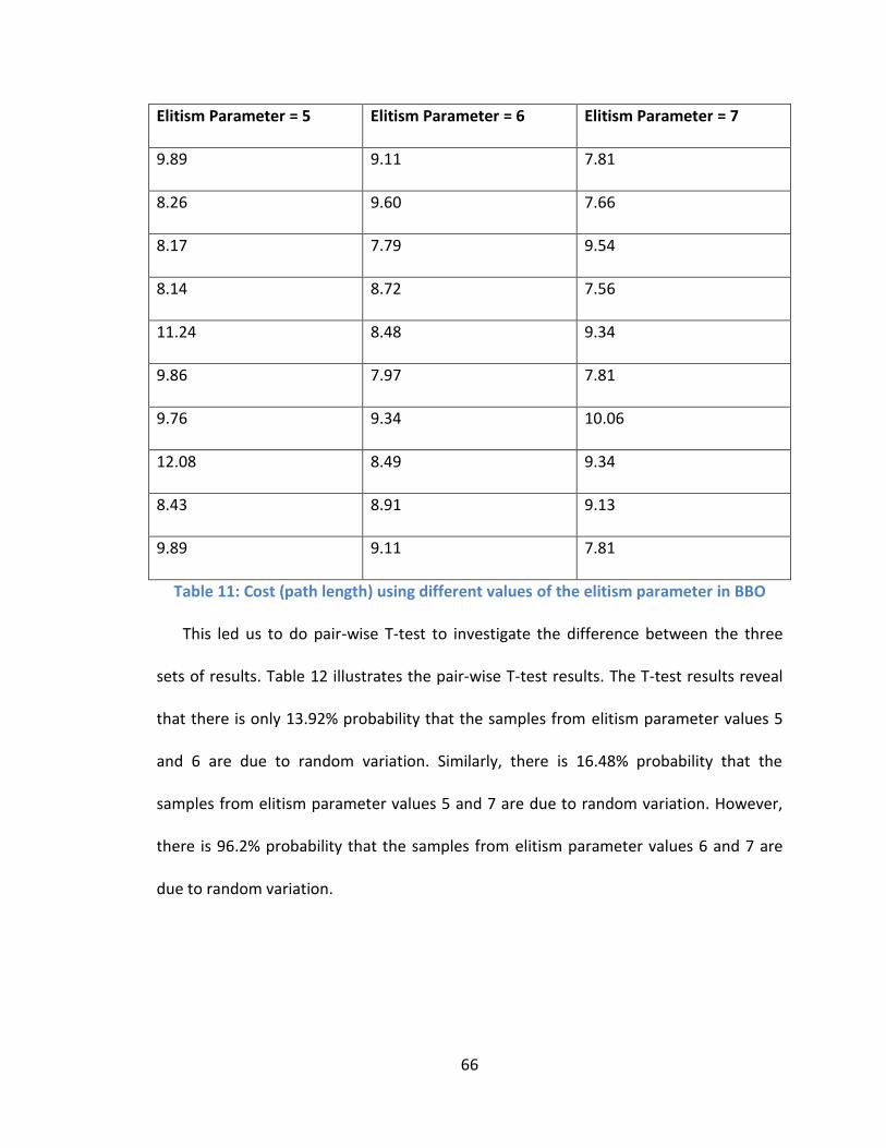
66
Elitism Parameter = 5 Elitism Parameter = 6 Elitism Parameter = 7
9.89 9.11 7.81
8.26 9.60 7.66
8.17 7.79 9.54
8.14 8.72 7.56
11.24 8.48 9.34
9.86 7.97 7.81
9.76 9.34 10.06
12.08 8.49 9.34
8.43 8.91 9.13
9.89 9.11 7.81
Table 11: Cost (path length) using different values of the elitism parameter in BBO
This led us to do pair-wise T-test to investigate the difference between the three
sets of results. Table 12 illustrates the pair-wise T-test results. The T-test results reveal
that there is only 13.92% probability that the samples from elitism parameter values 5
and 6 are due to random variation. Similarly, there is 16.48% probability that the
samples from elitism parameter values 5 and 7 are due to random variation. However,
there is 96.2% probability that the samples from elitism parameter values 6 and 7 are
due to random variation.
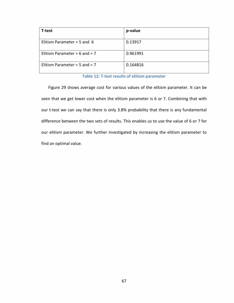
67
T-test p-value
Elitism Parameter = 5 and 6 0.13917
Elitism Parameter = 6 and = 7 0.961991
Elitism Parameter = 5 and = 7 0.164816
Table 12: T-test results of elitism parameter
Figure 29 shows average cost for various values of the elitism parameter. It can be
seen that we get lower cost when the elitism parameter is 6 or 7. Combining that with
our t-test we can say that there is only 3.8% probability that there is any fundamental
difference between the two sets of results. This enables us to use the value of 6 or 7 for
our elitism parameter. We further investigated by increasing the elitism parameter to
find an optimal value.
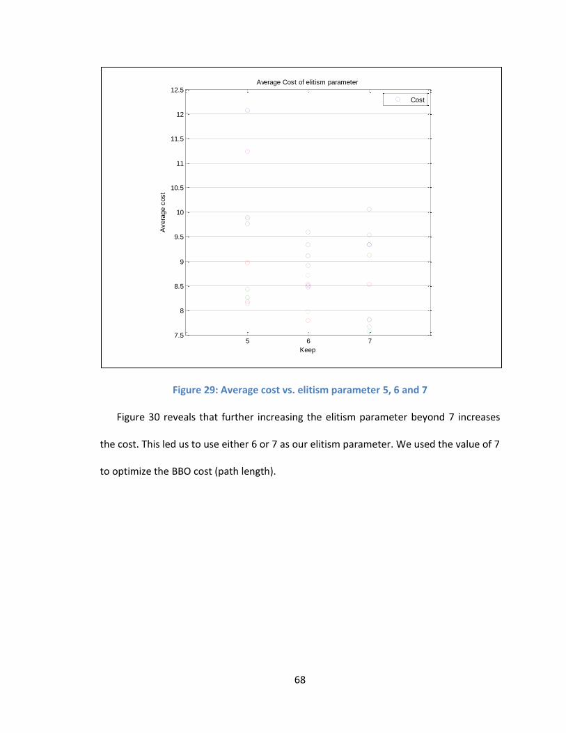
68
Figure 29: Average cost vs. elitism parameter 5, 6 and 7
Figure 30 reveals that further increasing the elitism parameter beyond 7 increases
the cost. This led us to use either 6 or 7 as our elitism parameter. We used the value of 7
to optimize the BBO cost (path length).
5 6 77.5
8
8.5
9
9.5
10
10.5
11
11.5
12
12.5
Keep
Avera
ge c
ost
Average Cost of elitism parameter
Cost
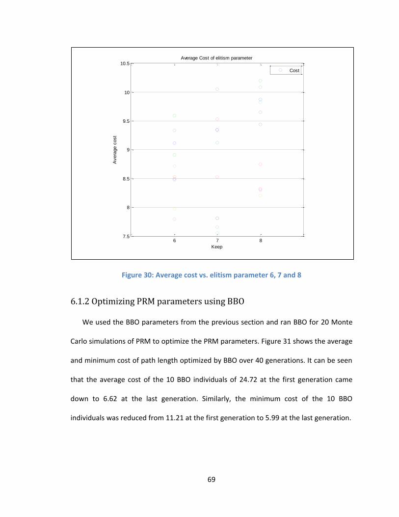
69
Figure 30: Average cost vs. elitism parameter 6, 7 and 8
6.1.2 Optimizing PRM parameters using BBO
We used the BBO parameters from the previous section and ran BBO for 20 Monte
Carlo simulations of PRM to optimize the PRM parameters. Figure 31 shows the average
and minimum cost of path length optimized by BBO over 40 generations. It can be seen
that the average cost of the 10 BBO individuals of 24.72 at the first generation came
down to 6.62 at the last generation. Similarly, the minimum cost of the 10 BBO
individuals was reduced from 11.21 at the first generation to 5.99 at the last generation.
6 7 87.5
8
8.5
9
9.5
10
10.5
Keep
Avera
ge c
ost
Average Cost of elitism parameter
Cost
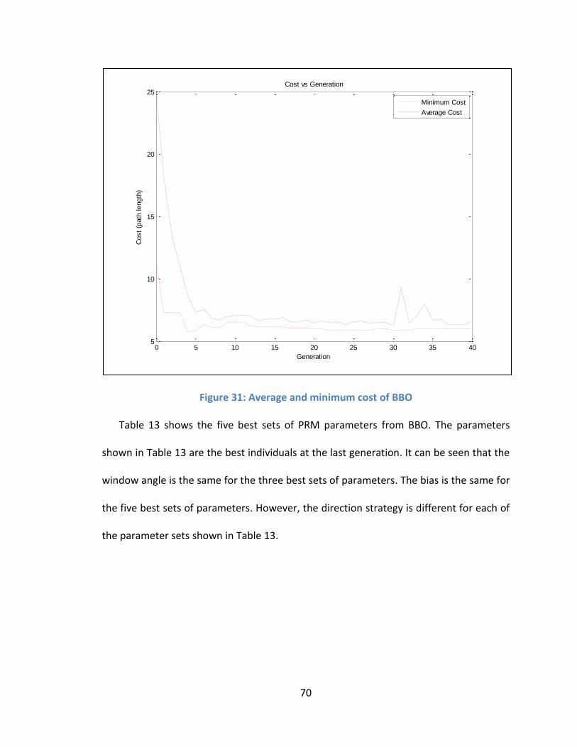
70
Figure 31: Average and minimum cost of BBO
Table 13 shows the five best sets of PRM parameters from BBO. The parameters
shown in Table 13 are the best individuals at the last generation. It can be seen that the
window angle is the same for the three best sets of parameters. The bias is the same for
the five best sets of parameters. However, the direction strategy is different for each of
the parameter sets shown in Table 13.
0 5 10 15 20 25 30 35 405
10
15
20
25
Generation
Cost
(path
length
)
Cost vs Generation
Minimum Cost
Average Cost
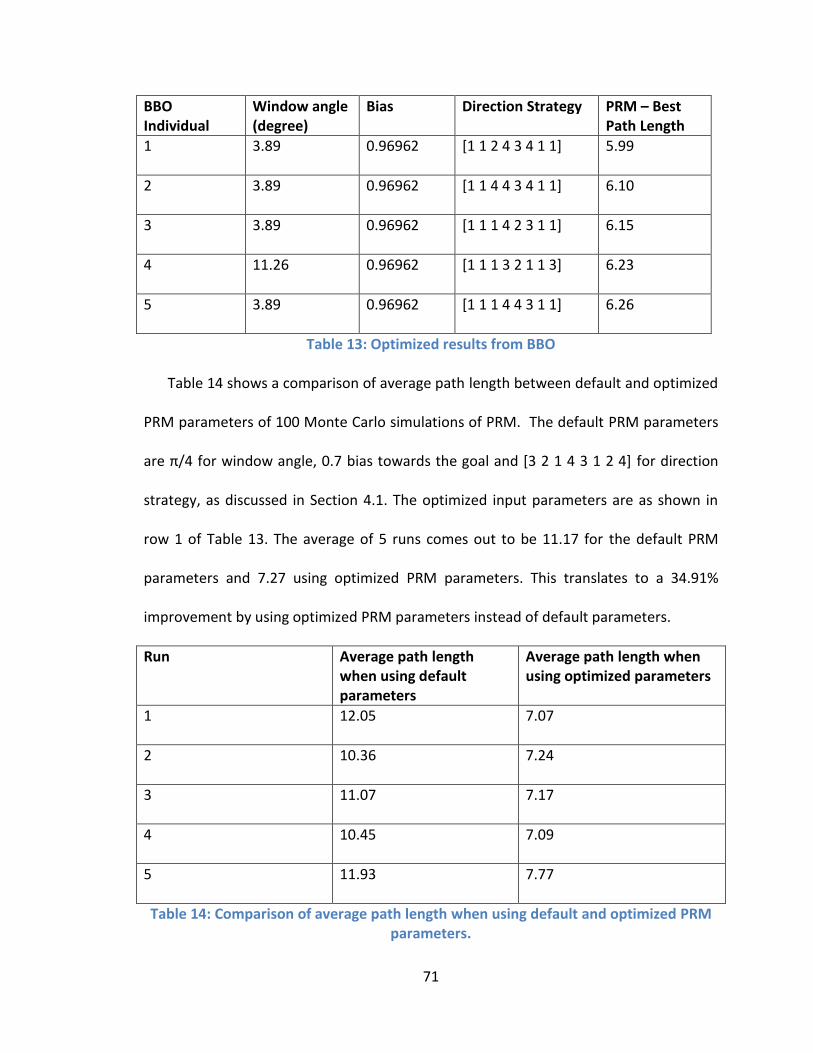
71
BBO Individual
Window angle (degree)
Bias Direction Strategy PRM – Best Path Length
1 3.89 0.96962 [1 1 2 4 3 4 1 1] 5.99
2 3.89 0.96962 [1 1 4 4 3 4 1 1] 6.10
3 3.89 0.96962 [1 1 1 4 2 3 1 1] 6.15
4 11.26 0.96962 [1 1 1 3 2 1 1 3] 6.23
5 3.89 0.96962 [1 1 1 4 4 3 1 1] 6.26
Table 13: Optimized results from BBO
Table 14 shows a comparison of average path length between default and optimized
PRM parameters of 100 Monte Carlo simulations of PRM. The default PRM parameters
are π/4 for window angle, 0.7 bias towards the goal and [3 2 1 4 3 1 2 4] for direction
strategy, as discussed in Section 4.1. The optimized input parameters are as shown in
row 1 of Table 13. The average of 5 runs comes out to be 11.17 for the default PRM
parameters and 7.27 using optimized PRM parameters. This translates to a 34.91%
improvement by using optimized PRM parameters instead of default parameters.
Run Average path length when using default parameters
Average path length when using optimized parameters
1 12.05 7.07
2 10.36 7.24
3 11.07 7.17
4 10.45 7.09
5 11.93 7.77
Table 14: Comparison of average path length when using default and optimized PRM parameters.
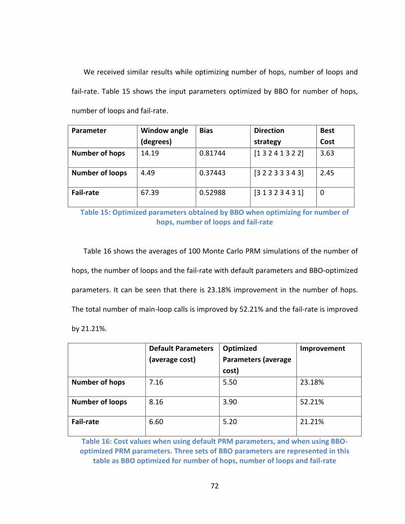
72
We received similar results while optimizing number of hops, number of loops and
fail-rate. Table 15 shows the input parameters optimized by BBO for number of hops,
number of loops and fail-rate.
Parameter Window angle
(degrees)
Bias Direction
strategy
Best
Cost
Number of hops 14.19 0.81744 [1 3 2 4 1 3 2 2] 3.63
Number of loops 4.49 0.37443 [3 2 2 3 3 3 4 3] 2.45
Fail-rate 67.39 0.52988 [3 1 3 2 3 4 3 1] 0
Table 15: Optimized parameters obtained by BBO when optimizing for number of hops, number of loops and fail-rate
Table 16 shows the averages of 100 Monte Carlo PRM simulations of the number of
hops, the number of loops and the fail-rate with default parameters and BBO-optimized
parameters. It can be seen that there is 23.18% improvement in the number of hops.
The total number of main-loop calls is improved by 52.21% and the fail-rate is improved
by 21.21%.
Default Parameters
(average cost)
Optimized
Parameters (average
cost)
Improvement
Number of hops 7.16 5.50 23.18%
Number of loops 8.16 3.90 52.21%
Fail-rate 6.60 5.20 21.21%
Table 16: Cost values when using default PRM parameters, and when using BBO-optimized PRM parameters. Three sets of BBO parameters are represented in this
table as BBO optimized for number of hops, number of loops and fail-rate

73
6.2 Experimental Results
We then used the input parameters optimized by BBO shown in the first row of
Table 13 to find the path between Cartesian coordinates (0.5, 0.5) and (2.5, 2.5). Figure
32 shows the path found by the optimized input parameters. We use two arbitrary,
predefined obstacles in the configuration space. The coordinates of the first obstacle are
(1.3, 1.1), (1.8, 1.5) and (1.0, 1.7) and the coordinates of the second obstacle are (2.1,
0.2), (2.4, 0.8) and (2.5, 0.3). The output of the PRM function is shown in Table 17.
Parameter Value
Path Length 3.5 units
Number of hops 5
Number of loops 15
Fail-rate 0%
Table 17: Output of PRM using input parameters optimized for path length
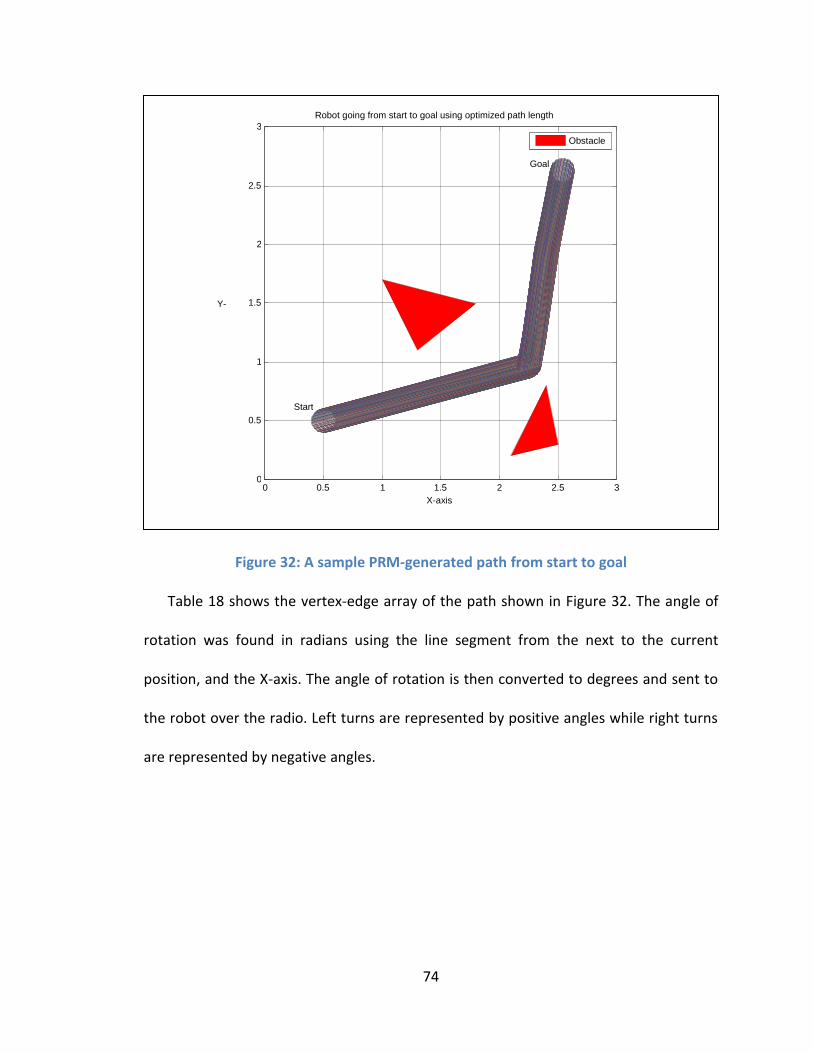
74
Figure 32: A sample PRM-generated path from start to goal
Table 18 shows the vertex-edge array of the path shown in Figure 32. The angle of
rotation was found in radians using the line segment from the next to the current
position, and the X-axis. The angle of rotation is then converted to degrees and sent to
the robot over the radio. Left turns are represented by positive angles while right turns
are represented by negative angles.
0 0.5 1 1.5 2 2.5 3 0
0.5
1
1.5
2
2.5
3
X-axis
Y-
axis
Robot going from start to goal using optimized path length
Obstacle
Start
Goal
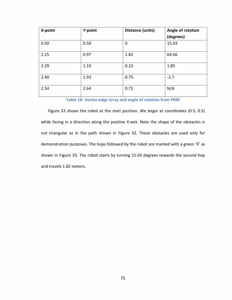
75
X-point Y-point Distance (units) Angle of rotation
(degrees)
0.50 0.50 0 15.03
2.25 0.97 1.82 64.66
2.29 1.19 0.23 1.85
2.40 1.93 0.75 -2.7
2.54 2.64 0.72 N/A
Table 18: Vertex-edge array and angle of rotation from PRM
Figure 33 shows the robot at the start position. We begin at coordinates (0.5, 0.5)
while facing in a direction along the positive X-axis. Note the shape of the obstacles is
not triangular as in the path shown in Figure 32. These obstacles are used only for
demonstration purposes. The hops followed by the robot are marked with a green ‘X’ as
shown in Figure 33. The robot starts by turning 15.03 degrees towards the second hop
and travels 1.82 meters.
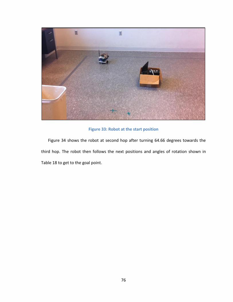
76
Figure 33: Robot at the start position
Figure 34 shows the robot at second hop after turning 64.66 degrees towards the
third hop. The robot then follows the next positions and angles of rotation shown in
Table 18 to get to the goal point.
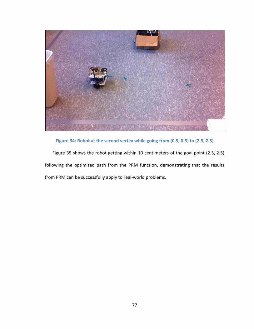
77
Figure 34: Robot at the second vertex while going from (0.5, 0.5) to (2.5, 2.5)
Figure 35 shows the robot getting within 10 centimeters of the goal point (2.5, 2.5)
following the optimized path from the PRM function, demonstrating that the results
from PRM can be successfully apply to real-world problems.
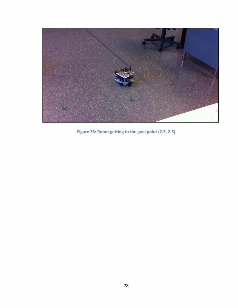
78
Figure 35: Robot getting to the goal point (2.5, 2.5)
79
CHAPTER VII
CONCLUSION AND FUTURE WORK
In this chapter all the relevant information covered in this research is summarized. In
this chapter we also shed some light on the limitations and scope of using optimization
for robot path planning. It has been shown that engineers can learn from the nature of
biological organisms, and that knowledge can be used to optimize complex engineering
problems.
7.1 Limitations and Scope
The limitations in robot path planning directly depend upon the resources involved.
Time and money are the major constraints in such a project. Use of better hardware will
ensure that the robot correctly follows the path developed by PRM and optimized by
BBO. The possibility and scope for research that addresses the path planning problem of
car-like robots are endless. Space exploration, driver-less cars and oceanographic
imaging are only a few examples where this technique can be applied.
80
The path planning algorithm can be enhanced on various scales such as
computational complexity and speed. After enhancing the input parameters using BBO,
the path planning algorithms can be tested in real-time environment. A combination of
dead-reckoning and additional hardware can be used to tackle real-world scenarios.
Camera, sensor, laser and sonar can be used in conjunction with information from
actual wheel movement to localize the robot. Additional memory can be utilized to save
the maps of already visited places. These maps can also be saved on a central server
which can then be shared among multiple mobile robots. Additional hardware will also
require more energy to run. A tradeoff will have to be made between the additional
hardware used in the robot and the overall capabilities of the robot.
7.2 Conclusion
We successfully implemented PRM for car-like robots in an obstacle filled
configuration space. The output from PRM, a vertex-edge array, was then transmitted to
the robot via radio. The demonstration shows the robot following the path found by
PRM.
We ran t-tests and F-tests to find the optimal BBO parameters. Those parameters
were then used in BBO to optimize PRM with respect to path length, number of hops,
number of loops and fail-rate. Section 6.1.2 showed that we achieved significant
improvements, ranging from approximately 21% to 52%, after using the optimized PRM
parameters.
This research shows that BBO can be used to optimize the parameters of path
planning algorithms. Our results demonstrate that the field of robot path planning can
81
benefit from evolutionary optimization algorithms. This work can be further extended to
multiple mobile-robots. The optimized parameters can be used to find the real-time
path in a configuration space with dynamic obstacles. Additional hardware can be used
to effectively tackle real-world robot path planning scenarios
7.3 Future Work
Our next suggested step is to implement a dynamic configuration space for car-like
robots. This will allow us to amend our system to make it closer to a real-world
situation. The robot code from the PIC microcontroller can also be modified to
implement reverse motion for the robot. Another step would be to use multiple robots
where a distributed biology-based optimization algorithm could be employed [21].
As discussed in the previous sections, we have multiple objectives that we are
optimizing using BBO. All of these objectives (path length, number of hops, number of
loops and fail-rate) are optimized independently from each another. A multi-objective
optimization algorithm to achieve Pareto optimality can be employed to find a desired
balance among the objectives [29]. Pareto optimality can be used when we have more
than one objective and it is not possible to make one of the objectives better without
making other objectives worse. A decision-maker is then able to find a balanced solution
from the Pareto front generated by the multi-objective optimization algorithm.
82
WORKS CITED
[1] H. Choset, "Coverage for Robotics - A Survey of Recent Results," Analysis of
Mathematics and Artificial Intelligence, vol. 31, pp. 113-126, 2001.
[2] R. Geraerts and M. Overmars, "A comparative study of probabilistic roadmap
planners," in Workshop on the Algorithmic Foundations of Robotics, Nice, France,
2002, pp. 43-57.
[3] N. Agmon, S. Kraus, and G. Kaminka, "Multi-Robot Perimeter Patrol in Adversarial
Settings," in IEEE International Conference on Robotics and Automation, Pasadena,
CA, 2008, pp. 2339-2345.
[4] P. Svestka and M. Overmars, "Motion Path Plannign for Car-like Robots using a
Probabilistic Learning Approach," International Journal of Robotics Research, pp.
119-143, 1997.
[5] K. Belghith, F. Kabanza, L. Hartman, and R. Nkambou, "Anytime Dynamic Path
Planning with Flexible Probabilistic Roadmaps," in IEEE International Conference on
Robotics and Automation, 2006, pp. 2372-2377.
[6] R. Al-Hmouz, T. Gulrez, and A. Al-Jumaily, "Probabilistic Road Maps with Obstacle
Avoidance in Cluttered Dynamic Environments," in Proc. of Intelligent Sensor,
Sensor Networks and Information Processing Conference, 2004, pp. 241-245.
[7] N. Amato, O. Bayazit, L. Dale, C. Jones, and D. Vallejo, "OBPRM: An Obstacle-Based
PRM for 3D Workspaces," in Robotics: The algorithmic perspective., 1998, pp. 155-
168.
83
[8] N. Amato and L. Dale, "Probabilistic Roadmap Methods are Embarrassingly
Parallel," in IEEE International Conference on Robotics and Automation, 1999, pp.
688-694.
[9] S. Carpin, "Randomized Motion Planning - A Tutorial," International Journal of
Robotics and Automation, vol. 3, no. 21, pp. 184-196, 2006.
[10] N. Amato and D. Xie, "A Kinematics-Based Probabilistic Roadmap Method for High
DOF Closed Chain Systems," Texas A&M University, Texas, Technical Report TR03-
007, 2003.
[11] N. Amato, O. Bayazit, L. Dale, C. Jones, and D. Vallejo, "Choosing good distance
metrics and local planners for probabilistic roadmap methods," in IEEE International
Conference on Robotics and Automation, 1998, pp. 630-637.
[12] Y. Wu, "An Obstacle-Based Probabilistic Roadmap Method for Path Planning," Texas
A&M University, Texas, Master's Thesis 1996.
[13] M. Saha, "Motion Planning With Probabilistic Roadmaps," Stanford University, PhD
Thesis 2006.
[14] P. Svestka and M. Overmars, "Coordinated Path Planning for Multiple Robots," in
Robotics and Autonomous Systems, 1998, pp. 125-152.
[15] L. Kavraki, P. Svestka, J. Latombe, and M. Overmars, "Probabilistic Roadmaps for
Path Planning in High-Dimensional Configuration Spaces," IEEE Transactions on
Robotics and Automation, vol. 12, no. 4, pp. 566-580, August 1996.
[16] J. Redding et al., "A Real-time Obstacle Detection and Reactive Path Planning
84
System for Autonomous Small-Scall Helicopters," in AIAA Guidance, Navigation and
Control Conference and Exhibit, Hilton Head, August 2007, pp. 20-23.
[17] J. Bruce and M. Veloso, "Real-Time Randomized Path Planning for Robot
Navigation," in IEEE International Conference on Intelligent Robots and Systems,
2002, pp. 2383-2388.
[18] Y. Elmaliach, N. Agmon, and G. Kaminka, "Multi-Robot Area Patrol under Frequency
Constraints," in IEEE International Conference on Robotics and Automation, 2007,
pp. 385-390.
[19] V. Boor, M. Overmars, and A. Stappen, "The gaussian sampling strategy for
probabilistic roadmap planners," in IEEE International Conference on Robotics and
Automation, Detriot, Michigan, 1999, pp. 1018-1023.
[20] D. Simon, "Biogeography-Based Optimization," IEEE Transactions on Evolutionary
Computation, vol. 12, no. 6, pp. 702-713, December 2008.
[21] A. Shah, "Distributed Biogeography Based Optimization for Mobile Robots,"
Cleveland State University, Cleveland, Master's Thesis 2012.
[22] T. Wilmot, "Intelligent Controls for a Semi-active Hydaulic Prosthetic Knee,"
Cleveland State University, Cleveland, Master's Thesis August 2011.
[23] C. Churavy et al., "Effective implementation of a mapping swarm of robots," IEEE
Potentials, pp. 28-33, July/August 2008.
[24] P. Lozovyy, G. Thomas, and D. Simon, "Biogeography-Based Optimization for Robot
Controller Tuning," in Computational Modeling and Simulation of Intellect, B.
85
Igelnik, Ed. USA: IGI Global, 2011, ch. 7, pp. 162-181.
[25] T. Green. (2008) Embedded systems programming with the PIC16F877. [Online].
http://academic.csuohio.edu/simond/courses/eec417/ESPWithThePIC16F877.pdf
[26] Y. Kanetkar, Let us C, 2nd ed. New Delhi, India: BPB Publications, 1996.
[27] Microchip Technology, PIC18F2420/2520/4420/4520., 2004.
[28] G. Lucas. (2001) The Rossum Project. [Online].
http://rossum.sourceforge.net/papers/DiffSteer/#d7
[29] D. Simon, Evolutionary Optimization Algorithms. New Jersey, United States of
America: John Wiley & Sons, Inc., 2013.
[30] A. Hayter, Probability and Statistics for engineers and scientists, 3rd ed. Belmont,
United States of America: Thomson Brooks/Cole, 2007.
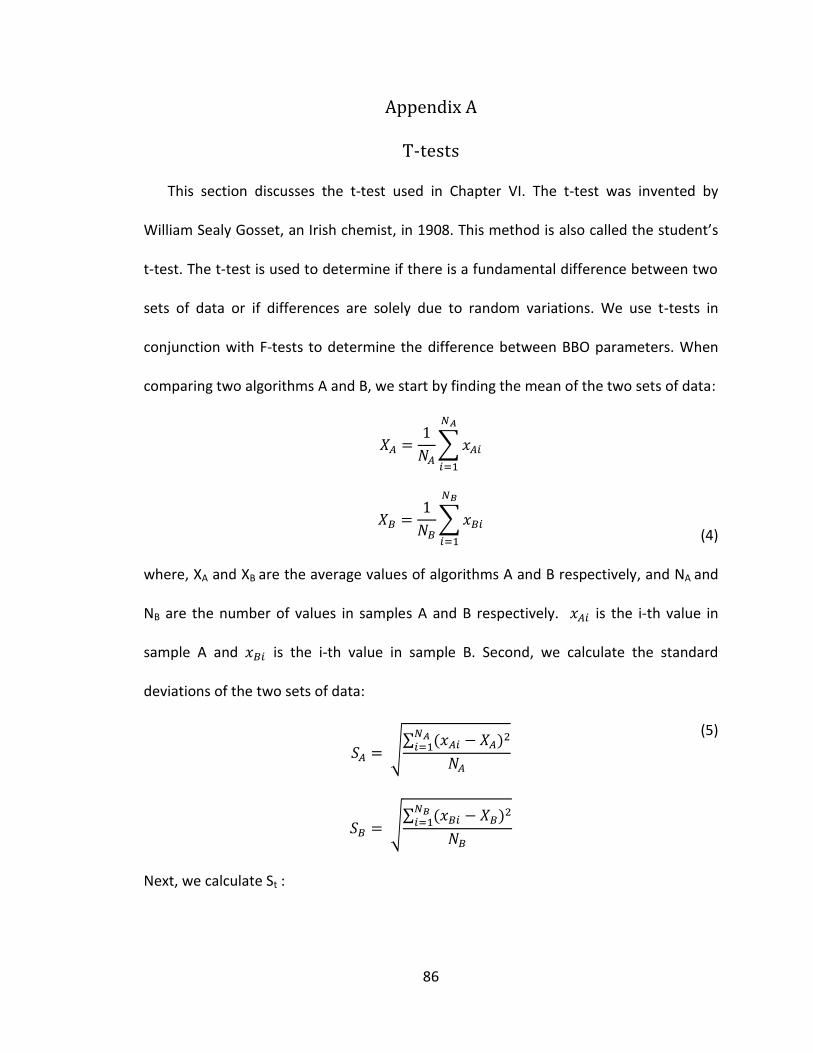
86
Appendix A
T-tests
This section discusses the t-test used in Chapter VI. The t-test was invented by
William Sealy Gosset, an Irish chemist, in 1908. This method is also called the student’s
t-test. The t-test is used to determine if there is a fundamental difference between two
sets of data or if differences are solely due to random variations. We use t-tests in
conjunction with F-tests to determine the difference between BBO parameters. When
comparing two algorithms A and B, we start by finding the mean of the two sets of data:
∑
∑
(4)
where, XA and XB are the average values of algorithms A and B respectively, and NA and
NB are the number of values in samples A and B respectively. is the i-th value in
sample A and is the i-th value in sample B. Second, we calculate the standard
deviations of the two sets of data:
√∑ ( )
√∑ ( )
(5)
Next, we calculate St :
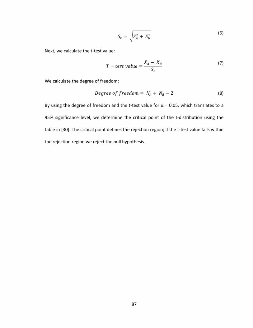
87
√
(6)
Next, we calculate the t-test value:
(7)
We calculate the degree of freedom:
(8)
By using the degree of freedom and the t-test value for α = 0.05, which translates to a
95% significance level, we determine the critical point of the t-distribution using the
table in [30]. The critical point defines the rejection region; if the t-test value falls within
the rejection region we reject the null hypothesis.
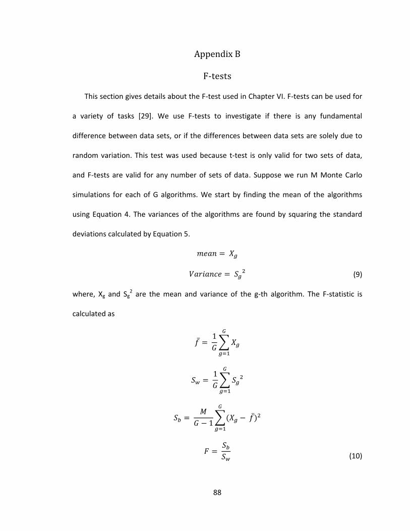
88
Appendix B
F-tests
This section gives details about the F-test used in Chapter VI. F-tests can be used for
a variety of tasks [29]. We use F-tests to investigate if there is any fundamental
difference between data sets, or if the differences between data sets are solely due to
random variation. This test was used because t-test is only valid for two sets of data,
and F-tests are valid for any number of sets of data. Suppose we run M Monte Carlo
simulations for each of G algorithms. We start by finding the mean of the algorithms
using Equation 4. The variances of the algorithms are found by squaring the standard
deviations calculated by Equation 5.
(9)
where, Xg and Sg2 are the mean and variance of the g-th algorithm. The F-statistic is
calculated as
∑
∑
∑( )
(10)
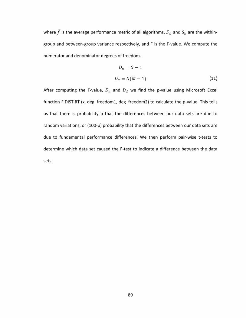
89
where is the average performance metric of all algorithms, and are the within-
group and between-group variance respectively, and F is the F-value. We compute the
numerator and denominator degrees of freedom.
( ) (11)
After computing the F-value, and we find the p-value using Microsoft Excel
function F.DIST.RT (x, deg_freedom1, deg_freedom2) to calculate the p-value. This tells
us that there is probability p that the differences between our data sets are due to
random variations, or (100-p) probability that the differences between our data sets are
due to fundamental performance differences. We then perform pair-wise t-tests to
determine which data set caused the F-test to indicate a difference between the data
sets.
Recommended


![Developing Multiple Topologies of Path Generating ... · PDF fileGenerating Compliant Mechanism (PGCM) using Evolutionary Optimization ... [23–26] and path generating ... generated](https://img.pdfslide.us/doc/110x75/5a84477c7f8b9a001c8b6ef2/developing-multiple-topologies-of-path-generating-compliant-mechanism-pgcm.jpg)