Dipartimento Interateneo di FisicaCorso di Laurea Magistrale in Fisica
TESI DI LAUREA MAGISTRALE
Particle models of atmospheric-pressuremicrodischarges in Ar and N2
Relatore: Laureando:Prof. Savino Longo Fabrizio PellegriniCorrelatore:Dott. Francesco Taccogna
Anno Accademico 2016/2017

Contents
Introduction 3
1 Physics of Plasmas and Discharges 6
1.1 Fluid approach and fundamental concepts . . . . . . . . . . . . . . . 9
1.1.1 Debye shielding . . . . . . . . . . . . . . . . . . . . . . . . . . 12
1.1.2 Plasma frequency . . . . . . . . . . . . . . . . . . . . . . . . . 14
1.2 Breakdown and discharge regimes . . . . . . . . . . . . . . . . . . . . 15
1.2.1 Townsend mechanism . . . . . . . . . . . . . . . . . . . . . . 16
1.2.2 Glow regime . . . . . . . . . . . . . . . . . . . . . . . . . . . . 20
1.2.3 Streamer mechanism . . . . . . . . . . . . . . . . . . . . . . . 24
1.2.4 Homogeneous vs lamentary mode in atmospheric pressure
discharges . . . . . . . . . . . . . . . . . . . . . . . . . . . . . 27
1.3 Sheaths . . . . . . . . . . . . . . . . . . . . . . . . . . . . . . . . . . 31
1.3.1 High voltage sheath . . . . . . . . . . . . . . . . . . . . . . . 34
1.4 Non-equilibrium in low-temperature plasmas at atmospheric pressure 36
2 Kinetic Simulation of Electric Discharges 40
2.1 Introduction . . . . . . . . . . . . . . . . . . . . . . . . . . . . . . . . 40
2.2 Overview of simulation methods . . . . . . . . . . . . . . . . . . . . 41
2.3 The Particle-In-Cell method . . . . . . . . . . . . . . . . . . . . . . . 45
2.3.1 The particle mover . . . . . . . . . . . . . . . . . . . . . . . . 51
2.3.2 Particle and eld weighting . . . . . . . . . . . . . . . . . . . 55
2
CONTENTS 3
2.3.3 The eld solver . . . . . . . . . . . . . . . . . . . . . . . . . . 58
2.4 The Monte Carlo Collision method . . . . . . . . . . . . . . . . . . . 60
3 Description of the PIC-MCC model developed 65
3.1 Physical system and numerical parameters . . . . . . . . . . . . . . . 65
3.2 Modelling of elementary processes: N2 . . . . . . . . . . . . . . . . . 68
3.2.1 Analytic cross sections for e−N2 collisions and e−N+2 recom-
binations . . . . . . . . . . . . . . . . . . . . . . . . . . . . . 69
3.2.2 Calculation of post-collision velocities in e−N2 collisions . . 70
3.2.3 The Nanbu-Kitatani model for ion-neutral collisions . . . . . 72
3.3 Modelling of elementary processes: Ar . . . . . . . . . . . . . . . . . 76
4 Simulation results 77
4.1 Streamer evolution . . . . . . . . . . . . . . . . . . . . . . . . . . . . 77
4.2 Streamer spatial structure . . . . . . . . . . . . . . . . . . . . . . . . 82
4.3 Comparison among dierent cases . . . . . . . . . . . . . . . . . . . . 87
Conclusions 89
A Cross sections data 91
B Box-Muller transform 94

Introduction
This thesis work is concerned with the computer simulation of electric discharges at
atmospheric pressure.
Electric discharges consist essentially in the ionization of a previously non-conducting
gaseous medium, caused by the application of a suciently large electric eld which
accelerates free charged particles. The electric breakdown which follows leads to
the creation of a plasma, i.e. a mixture of electrons, ions and neutral atoms or
molecules. Plasmas are a complicating but fascinating subject, because of the variety
of behaviours that they can show depending on the conditions under which they
evolve. Electric discharges can be observed in nature (lightnings, blue jets, sprites)
or can be produced articially, in the laboratory. At atmospheric pressure, the main
advantage is that a vacuum system is not required; this makes possible the use of
these kind of discharges in the biomedical eld, or in the aerodynamic control for
airplane wings, for example.
Historically, electric discharges were studied in the laboratory starting from the last
decades of 1800, using low-pressure vacuum tubes.
The work of J. S. Townsend (who collaborated with J. J. Thomson) at the turn of
the century was very important in order to provide the rst quantitative treatment
of electric breakdown in a gas. His theory was used successfully until some severe
discrepancies with experimental results at high pressure led to the development of a
theory based on a dierent breakdown mechanism (i.e. streamer), due to the work
of J. M. Meek in the 40's.
4

The mathematical treatment of highly collisional plasmas is very complicated, there-
fore computer simulations oer an ideal tool to investigate their properties. In par-
ticular, the Particle-In-Cell method which will be used in this work is based on a
kinetic approach which allows large spatial and temporal resolution, while providing
precious information about non-equilibrium of the dierent species involved. Colli-
sional processes among charged and neutral species will be treated with the Monte
Carlo Collision method, i.e. a stochastic approach.
This is the outline of this thesis work:
• Chapter 1: it deals with some general concepts about plasmas, provides a short
introduction to the uid approach and introduces the fundamental length and
time scales in plasma physics. Furthermore, the two main mechanisms of elec-
tric breakdown are explained, sheaths (i.e. the boundary region which connects
a plasma with a wall or an electrode) are considered. The last paragraph deals
with non equilibrium at atmospheric pressure.
• Chapter 2: after a brief overview of the possible choices of simulation methods,
the Particle-In-Cell and Monte Carlo Collision methods are described in detail.
In particular, the PIC is given a sound mathematical basis.
• Chapter 3: the main features of the model developed in order to simulate a
dielectric barrier discharge (DBD) powered by a nanosecond voltage pulse are
described. The dynamics at the nanosecond timescale is still poorly under-
stood, and the interest of the plasma community has ourished only in the last
decade.
In the last two paragraphs, the treatment of collisional processes is explained
for the two case study gases, N2 and Ar.
• Chapter 4: in the last chapter, we present the results of our simulations.
5

Chapter 1
Physics of Plasmas and Discharges
Plasmas are usually referred to as the fourth state of matter. The meaning of this
sentence can be understood if we think that heating a solid, it undergoes a phase
transition becoming a liquid; further heating causes the liquid-gas phase transition.
At temperatures as high as tens of thousands K, electrons are stripped from neutral
atoms and molecules by collisional processes, and a plasma is formed.
A plasma can so be dened as a mixture of electrons, positively ionized and neutral
species, which preserves quasi-neutrality and shows collective behavior. [1]
What we mean by collective behavior and quasi-neutrality will become clearer in
the next paragraph, but qualitatively collective behavior is a consequence of the
Coulomb force which acts upon charged particles: while in a neutral gas particles
interact essentially only through forces which are very short-range, every region of a
plasma is aected by far away regions. Information does not propagate only through
collisions, but also through electromagnetic elds. Quasi-neutrality means that,
although a plasma is neutral as a whole, charge density can be dierent from zero,
on a suciently small scale (Debye length, see 1.1.1). As a result, large electric elds
develop in order to restore neutrality.
Plasmas are ubiquitous in nature: they can be found in stars, interstellar space,
planetary atmospheres (ionosphere), lightnings. They can also be produced arti-
cially in electrical discharges, by applying a suciently strong electromagnetic eld,
so that free electrons gain enough energy, in a mean free path, to ionize atoms and
molecules. Fig.1.1 shows a schematic representation of a typical discharge tube. It
can be lled with various gases.
6

CHAPTER 1. PHYSICS OF PLASMAS AND DISCHARGES 7
Figure 1.1: Schematic view of a discharge tube (Raizer, [2])
Electrical discharges and their simulation will be the subject of this thesis work;
they are often characterized by the fact that electrons, ions and neutrals can have
dierent temperatures, i.e. they are non-equilibrium plasmas.. Although the rela-
tionship between dierent plasma temperatures in non-thermal plasmas can be quite
sophisticated, it can be conventionally presented in collisional weakly ionized plas-
mas as Te > Tv > Tr ≈ Ti ≈ T0. This means that the highest temperature is that
of electrons (of the order of a few eV, i.e. tens of thousands of K), followed by that
of vibrational degrees of freedom of molecules, while rotational degrees of freedom,
ions and neutrals usually share the room temperature (of the order of tens of meV).
On the contrary, plasmas in stars or in fusion reactors are thermal plasmas, and all
the species can be considered to have the same temperature.
Plasmas produced in gas discharges can be used for a great variety of applications.
We may subdivide them in volume and surface processes.
In the former case, plasmas can be seen as chemical reactors. In fact, excited species
created through collisions are most eciently converted into nal products. As an
example, we can mention CO2 dissociation into CO+O. This can be done with
high-energy eciency and high selectivity in a cold discharge. In fact, electrons
with energies around 1 eV primarily transfer their energy into molecular vibrational
excitations. In this way, it is possible to selectively introduce up to 90% of the total
discharge power in CO production. Electronically excited metastable states also
have a signicant role in plasma chemistry, for example oxygen molecules O2(1∆g)
(singlet oxygen), which eectively participate in the plasma-stimulated oxidation
process in polymer processing, and biological and medical applications [3].
Plasmas are also used to modify the surface properties of materials. Plasma-based
surface processes are indispensable for manufacturing the integrated circuits (ICs)
used by the electronics industry. For microfabrication of an IC, one-third of the
tens to hundreds of fabrication steps are typically based on discharge application.
Silicon etching, i.e. the process through which layers of a silicon wafer are removed,
CHAPTER 1. PHYSICS OF PLASMAS AND DISCHARGES 8
is among the dierent processes the most important. Following Lieberman [4], we
can etch silicon starting with an inert molecular gas, CF4, and sustain a discharge
through electron-neutral dissociative ionization:
e+ CF4 → 2e+ CF+3 + F.
Then, a highly-reactive species is created by electronneutral dissociation:
e+ CF4 → e+ F + CF3 → e+ 2F + CF2
In this case, the etching species is atomic uoride: it reacts with solid silicon, yielding
the volatile etch product SF4:
Si(s) + 4F (g) → SiF4(g)
This nal product is then pumped away.
In the way we have just described, silicon is etched isotropically. If we use CF+3
ions to bombard the substrate, a directional/anisotropic etching can be obtained.
In addition, one can control reactive species densities, their energies and uxes to
the targets. So, a detailed knowledge of the fundamental processes by which these
species are created is required. Also, a knowledge of gas-phase and surface chemistry
is needed.
In this work, the streamer regime will result as a fundamental mechanism to sustain
the electrical breakdown in atmospheric pressure discharges; they are involved in nu-
merous natural phenomena: lightnings, sprites observed between about 40 and 90 km
height in the mesosphere and blue jets in the higher regions of the atmosphere above
thunderclouds (stratosphere). Due to their peculiar nature, the streamer regime is
characterized by a high production rate of reactive species and strong movement
of space charge regions. For these reasons, they are also used in dierent techno-
logical applications ranging from chemical (production of ozone, CO2 conversion)
to biomedical (living tissues treatment and plasma-cellular membrane electrophore-
sis), energy (plasma-assisted ignition and combustion) and hydrodynamic (plasma
actuator and ame control) uses.

CHAPTER 1. PHYSICS OF PLASMAS AND DISCHARGES 9
1.1 Fluid approach and fundamental concepts
We want to introduce now some very basic concepts in plasma physics. In order to
do so, we need to acquire some knowledge of the so-called uid approach, which is
a simplied, although very useful, description of the behavior of a system composed
of a large number of particles. Its main disadvantage is that all kinetic information
are missed. We will return to simulation issues in the next chapter.
The statistical description of an ensemble of a large number of particles is usually
made in terms of a distribution function dened in the single particle phase-space,
fα(r,v, t), where the subscript is referred to the species α.
It is dened so that fα(r,v, t) d3r d3v represents the number of particles with velocity
in [v,v + dv] and position in [r, r + dr].
The distribution function obeys Boltzmann's equation (we will drop the index of
the species for the remainder of this paragraph):
∂f
∂t+ v · ∇rf + a · ∇vf =
(∂f
∂t
)c
(1.1)
where a is the particle acceleration, and the right-hand side represents the eect of
collisions, i.e. particle-particle interactions. It takes into account elastic and inelastic
processes.
Being interested in plasmas, where external forces are electromagnetic, (1.1) takes
the form:
∂f
∂t+ v · ∇rf +
q
m(E + v ×B) · ∇vf =
(∂f
∂t
)c
(1.2)
The exact knowledge of the state of a plasma is based on the solution of the previous
equation. This is notoriously a very hard task. The thermal equilibrium solution is
well known, i.e. the Maxwell distribution.
As we anticipated, a description of the system can be made on the basis of a simplied
set of equations in which few macroscopic variables appear. These equations can be
derived by taking the rst velocity moments of Boltzmann's equation. In other
words, we want to drop the particle velocities dependence from our description of
the system.

CHAPTER 1. PHYSICS OF PLASMAS AND DISCHARGES 10
• Continuity equation
By taking the integral of (1.2) over velocity space, the last term on the lhs vanishes
and so does the rhs if there are no source or loss processes, leading to:
∫ (∂f
∂t+ v · ∇rf
)d3v = 0
Recalling that the zeroth and rst order moment of the distribution are the particle
number density and particle ux, respectively, we get:
∂n
∂t+∇r · (nu) = 0 (1.3)
This is the continuity equation. If there is contribution from ionization (i.e. density
sources) and recombination or boundary absorption (i.e. density losses), their rate
is to be added consistently to the rhs.
• Momentum transfer equation
Multiplying (1.2) by v, integrating over velocity space and using the continuity
equation, we get:
mn
[∂u
∂t+ u · ∇u
]= qn(E + u×B)−∇ ·Π+ f c (1.4)
The second term on the rhs is the force density due to the divergence of the stress
tensor, which is dened as:
Πij = m ⟨(vi − u)(vj − u)⟩
where the term in brackets is averaged over the distribution; i and j are two cartesian
directions.
In the case of an isotropic distribution (e.g. absence of magnetic elds) the stress
tensor becomes diagonal:
Π =
p 0 0
0 p 0
0 0 p

CHAPTER 1. PHYSICS OF PLASMAS AND DISCHARGES 11
where p is the pressure; in this case, the simple gradient of p appears in the momen-
tum transfer equation.
The collisional term can be very complicated; in most uid treatment, it is approxi-
mated by:
fc = −mn(u− u0)
τc
where u0 is the mean velocity of the dominant species (neutrals, in weakly ionized
plasmas) and τc is the mean free time between collisions.
Equation (1.4) can be compared with Navier-Stokes equation in ordinary hydrody-
namics:
ϱ
[∂u
∂t+ u · ∇u
]= −∇p+ ϱν∇2u (1.5)
The last term in the rhs, where ν is the kinematic viscosity coecient, is the viscosity
term. The two equations are formally identical, except for the electromagnetic term.
• Energy conservation
The last equation describing the plasma in the uid approach is the energy conser-
vation equation. It is obtained by multiplying by 12mv2 Boltzmann's equation and
integrating.
It can be written in the following form:
∂
∂t
(3
2p
)+∇ ·
(3
2pu
)+ p∇ · u+∇ · J =
∂
∂t
(3
2p
)c
(1.6)
where 32p is the thermal energy density, 3
2pu is the macroscopic thermal energy
ux, the third term gives the heating or cooling of the uid due to compression or
expansion of its volume, J is the microscopic thermal energy ux, usually modeled
by −kT∇T (Fourier law) and the rhs is the time variation of thermal energy density
due to collisions.
The set of equations (1.3), (1.4) and (1.6), one for each species, must be closed with
Maxwell's equations, if the electromagnetic eld must be calculated self-consistently.
The last step consists in obtaining Boltzmann's relation, which expresses the density
of electrons as a function of electrostatic potential.

CHAPTER 1. PHYSICS OF PLASMAS AND DISCHARGES 12
Boltzmann's relation
Let's start from the uid equation of motion for electrons in an electric eld, assuming
an unmagnetized plasma:
mne
[∂u
∂t+ u · ∇u
]= −eneE−∇p+ fc (1.7)
Assuming collisions negligible and that there's no drift (u=0), the previous equation
becomes:
eneE+∇p = 0
If electrons can be considered isothermal, then p = nekTe. By substituting this
relation and E = −∇ϕ, we get:
ene∇ϕ−∇(nekTe) = 0
i.e. e∇ϕ = kTe∇(ln ne).
Integrating, we get:
ne(r) = n0eeϕ(r)kTe (1.8)
where n0 is the density where the potential is 0. This is Boltzmann's relation. It
reects the tendency of electrons to move towards regions of positive potential.
We are now in a position to introduce the fundamental length and time scales of
plasma physics.
1.1.1 Debye shielding
We can use Boltmann's relation to determine the characteristic length scale of electric
elds shielding in a plasma. This is our rst example of collective behavior.
Suppose we introduce a negatively charged sheet in an innitely extended plasma,
at x=0. We will also assume innitely massive singly charged ions, so that they can
be considered as forming a 'frozen' positive charge backgroung; instead, electrons
move away as they are repelled from the sheet.
CHAPTER 1. PHYSICS OF PLASMAS AND DISCHARGES 13
In the direction x perpendicular to the sheet, Poisson's equation can be written as:
d2ϕ
dx2=
e
ϵ0(ne − ni)
Using Boltzmann's relation for electrons density, and setting ni = n0 (ions are
unpertubed) we get:
d2ϕ
dx2=
en0
ϵ0
(e
eϕ(x)kTe − 1
)Supposing eϕ ≪ kTe, by a Taylor expansion which neglects second and higher order
terms:
d2ϕ
dx2=
e2n0
ϵ0kTeϕ
The solution satisfying boundary condition (ϕ(|x| → 0) = ϕ0 and ϕ(|x| → ∞) = 0)
is:
ϕ(x) = ϕ0e− x
λD (1.9)
where λD is called Debye length and is dened as:
λD =
√ϵ0kTe
e2n0(1.10)
From (1.9), it is clear that the Debye length is a measure of the length scale over
which external charges or elds eects are screened.
Another simple example of Debye shielding is given by thinking of a point charge
immersed in the plasma; in this case, its electric potential doesn't decrease as r−1,
but has a Yukawa form: r−1e−r/λD .
Debye shielding gives us the chance of understanding quasi-neutrality, as well.
Let's consider what happens on length scales l ≫ λD: Poisson's equation can be
written approximately as ϕl2
∼∣∣∣ eϵ0(ni − ne)
∣∣∣. Moreover, we can write ϕ ∼ kTee =
eϵ0neλ
2D. Plugging this into Poisson's equation and considering our scale length, we
obtain:
CHAPTER 1. PHYSICS OF PLASMAS AND DISCHARGES 14
|ni − ne| ≪ ne
That is to say, the plasma can be considered neutral on length scales much greater
than Debye length.
A more rened expression of Debye length which can be derived considering ions as
mobile species is:
λD =
√ϵ0k/e2
ne/Te +∑
i z2i ni/Ti
where ni, zie and Ti are the i-th ion species density, charge and temperature, respec-
tively.
1.1.2 Plasma frequency
Plasma frequency
If the Debye length is the fundamental length scale in plasma physics, what can be
said about timescales?
As we will see later, dierent timescales exist and must be taken into consideration
according to our particular interest. However, plasma frequency is certainly one of
the most important, and will be fundamental for our future task (i.e. computer
simulation of electrical discharges).
Plasma frequency is a concept which naturally emerges if one considers the following
elementary theory of plasma electron oscillations in one dimension: suppose ions
are frozen as in the previous section, and electrons neutralize them, at rst. Let's
neglect ions and electrons thermal motion, and suppose charge neutrality is disturbed
by displacing electrons from their equilibrium positions by an amount ζ(x) .
Consider the parallel planes at x1 and x2 and the electrons displaced into the volume
bounded by x1 + ζ1 and x2 + ζ2.
As a consequence of this displacement, the change in electron density can be written
as:
∆ne = −neζ2 − ζ1x2 − x1

CHAPTER 1. PHYSICS OF PLASMAS AND DISCHARGES 15
if, as we suppose, ζ ≪ x2 − x1.
By taking the limit, we get:
∆ne = −ne∂ζ
∂x
Now we use this expression in Poisson's equation as a source for the electric eld:
∂E
∂x= −e∆ne
ϵ0=
nee
ϵ0
∂ζ
∂x
The electric eld generated by the displacement can thus be written as E = neϵ0ζ.
This eld can be plugged into the equation of motion for the electrons:
d2ζ
dt2= − nee
2
meϵ0ζ (1.11)
Equation (1.11) shows that electrons oscillate harmonically about their equilibrium
position with a characteristic frequency given by:
ωp =
√nee2
meϵ0(1.12)
This is called plasma frequency ; we see that it increases with plasma density.
Considering a density value of 1016m−3, we get a frequency of the order of 1 GHz,
in the microwaves. This will be a lower bound for our case of interest.
Strictly speaking, our previous equation denes the electron plasma frequency. Also
ions have their own plasma frequency, which will be much smaller than that of
electrons because of their mass.
1.2 Breakdown and discharge regimes
In this paragraph we want to illustrate the fundamental process of electrical break-
down, which consists in the transition from an insulating gaseous medium to a con-
ducting one. This transition is caused by ionization, through collisions, of the initially
non-conducting gas.
We will consider Townsend mechanism at rst, followed by an introduction to the
CHAPTER 1. PHYSICS OF PLASMAS AND DISCHARGES 16
main features of the glow discharge regime, which constitutes the diuse opera-
tional mode of atmospheric pressure discharges. Then, we will focus on avalanche-
to-streamer transition; streamers are at the basis of the lamentary operational mode
of atmospheric pressure discharges.
1.2.1 Townsend mechanism
Suppose we apply a potential dierence between two electrodes separated by a gap d.
If this potential is under a certain threshold value, the only current which reaches the
electrodes is that due to the charge carriers always present in a gaseous medium and
produced by radioactivity or photoionization. This current is negligibly small, and
rapidly saturates because no new charges are produced during the electrons drift.
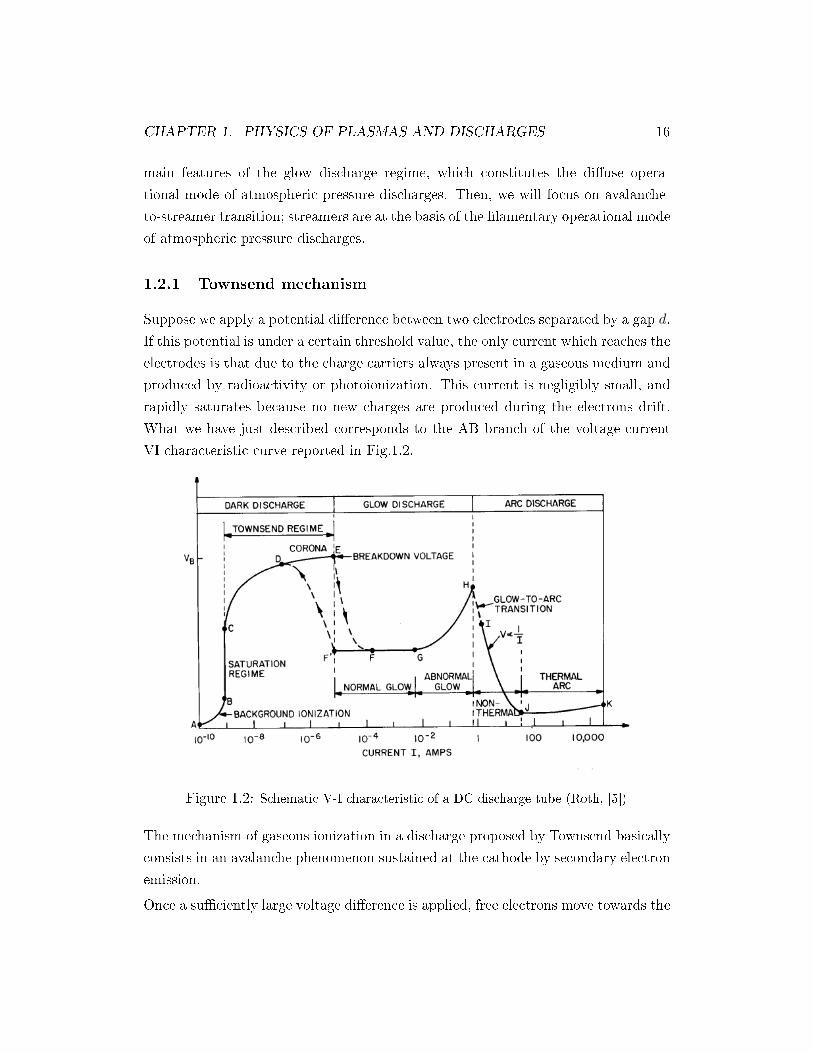
What we have just described corresponds to the AB branch of the voltage-current
VI characteristic curve reported in Fig.1.2.
Figure 1.2: Schematic V-I characteristic of a DC discharge tube (Roth, [5])
The mechanism of gaseous ionization in a discharge proposed by Townsend basically
consists in an avalanche phenomenon sustained at the cathode by secondary electron
emission.
Once a suciently large voltage dierence is applied, free electrons move towards the
CHAPTER 1. PHYSICS OF PLASMAS AND DISCHARGES 17
anode and gain enough energy to ionize neutral molecules or atoms. The electrons
produced, in turn, ionize other neutrals and so on, leading to an amplication of the
free charge carriers. Ions drift towards the cathode and, once they reach it, secondary
emission of electrons takes place. The current correspondingly grows by orders of
magnitude, but tipically remains quite small. This regime corresponds to the CE
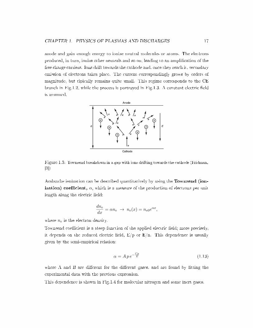
branch in Fig.1.2, while the process is portrayed in Fig.1.3. A constant electric eld
is assumed.
Figure 1.3: Townsend breakdown in a gap with ions drifting towards the cathode (Fridman,
[3])
Avalanche ionization can be described quantitatively by using the Townsend (ion-
ization) coecient, α, which is a measure of the production of electrons per unit
length along the electric eld:
dne
dx= αne → ne(x) = ne0e
αx,
where ne is the electron density.
Townsend coecient is a steep function of the applied electric eld; more precisely,
it depends on the reduced electric eld, E/p or E/n. This dependence is usually
given by the semi-empirical relation:
α = Ap e−CpE (1.13)
where A and B are dierent for the dierent gases, and are found by tting the
experimental data with the previous expression.
This dependence is shown in Fig.1.4 for molecular nitrogen and some inert gases.

CHAPTER 1. PHYSICS OF PLASMAS AND DISCHARGES 18
Figure 1.4: Experimental values of Townsend coecient for inert (left) and molecular
(right) gases (Lozansky [6], von Engel [7])
An analytical condition for Townsend breakdown can be derived in the following
way: each primary electron generated near the cathode produces eαd1 positive
ions, which move back to the cathode itself. By their impact, these ions extract
γ(eαd1) electrons, where γ is the ion-induced secondary electron emission coecient
(typically in the 0.01-0.1 range). If we call i0 the primary electron current, we can
write, for the total electron current at the cathode:
icath = i0 + icathγ(eαd1)
On the other hand, the total current at the anode is due only to the amplication
of the cathode electron current:
i = icatheαd
By combining the two previous relations, we get the Townsend formula for the total
current in the external circuit:
i =i0e
αd
1− γ(eαd1)(1.14)
When the denominator is positive, the discharge is in non-self-sustaining regime;
Townsend criterion for the breakdown is that the denominator goes to zero:

CHAPTER 1. PHYSICS OF PLASMAS AND DISCHARGES 19
Figure 1.5: Paschen curves for dierent atomic and molecular gases (Raizer, [2])
γ(eαd1) = 1 → α(Eb) =1
dln
(1
γ+ 1
)(1.15)
In the last equation of (1.15), Eb is the breakdown electric eld, i.e. the critical value
for which the current is self-sustained.
The physical interpretation of the criterion expressed by the rst equation of (1.15)
is that the ions ux at the cathode caused by a single primary electron leads to the
emission of one secondary electron on average. In this way, the discharge is indipen-
dent from external ionization phenomenon and can be considered self-sustained; if
γ(eαd1) < 1, on the contrary, the discharge is dependent on external sources of
ionization.
If we combine Eqs. (1.13) and (1.15), we get a very important and classical result,
i.e. the dependence of the breakdown potential, Vb = Eb d, from the product of
pressure and gap size:
Vb =B(pd)
C + ln(pd)(1.16)
where C = lnA − ln(ln
(1γ + 1
))is almost a constant. This relation is called
Paschen law, and is shown graphically in Fig.1.5 for some atomic and molecular
gases.

CHAPTER 1. PHYSICS OF PLASMAS AND DISCHARGES 20
It is interesting to note that it has a minimum, also known as Stoletov point,
which corresponds to the most ecient conditions for breakdown. The minimum
is expected because, as pressure is increased, the mean-free-path between ionizing
collisions decreases and so a stronger eld is required to sustain the discharge; the
same conclusion holds at lower pressures, but this time because there are fewer
collisions per electron.
Townsend disharges are usually called 'dark' discharges, because they are charac-
terised by such weak currents (less than 10−4A) that no appreciable light emission
occurs.
1.2.2 Glow regime
The term glow is historically used to describe a kind of low-pressure DC regime,
and the treatment which follows is essentially referred to this situation; on the other
hand, we will be concerned with high pressure discharges powered by very short
voltage pulses. Nonetheless, some of the features which we describe here have been
found to be useful in the context of high pressure discharges as well.
In Fig.1.6, the typical pattern of bright and dark layers of a DC glow discharge at
steady state is represented, together with the qualitative distribution of the most
important physical parameters. The two main regions in a glow discharge are the
cathode layer and the positive column. The former is found close to the cathode and
consists of Aston dark space, cathode glow and cathode dark space; the latter is a
region of quasi-neutral, weakly-ionized, non-equilibrium plasma, whose presence is
not mandatory and develops only if the gap is suciently large. The length of the
cathode layer varies roughly as p−1, so it can be found also in microdischarges at
atmospheric pressure, where gaps can be as small as hundreds of micrometers.
The glow regime is sustained by cathode secondary emission due to ionic impact,
similarly to a dark discharge. What sets the two regimes apart is the strong electric
eld distortion, due to space-charge eects in the cathode region of a glow discharge,
while currents and charge densities in a dark discharge are so small that the external
electric eld remains uniform along the entire gap length. The charge distribution,
as evident in Fig.1.6, gives rise to a large electric eld near the cathode; it then
decreases and eventually cancels at the end of the negative glow.
In order to understand the transition from a dark to a glow discharge, we can start

CHAPTER 1. PHYSICS OF PLASMAS AND DISCHARGES 21
Figure 1.6: DC glow discharge layers and potential, electric eld magnitude, current density
and charge distributions (Fridman, [3])
CHAPTER 1. PHYSICS OF PLASMAS AND DISCHARGES 22
with Townsend's mechanism. The following relations for electronic and ion currents
are easily obtained at steady state ([2], par. 8.3.1):
jej
= e−α(d−x),j+j
= 1− e−α(d−x),j+je
= eα(d−x) − 1 (1.17)
where x is the distance from cathode and j, the total current, is constant across the
gap. One clearly sees that the ionic current is larger then the electronic one in the
vicinity of the cathode; In fact, typically eαd ≫ 1. The dierence between ionic and
electronic densities is even greater because of the dierence in mobilities:
n+
ne=
µej+µ+je
(1.18)
Ions mobility can be hundreds of times smaller than electron mobility, so that close
to the cathode, n+ ≫ ne.
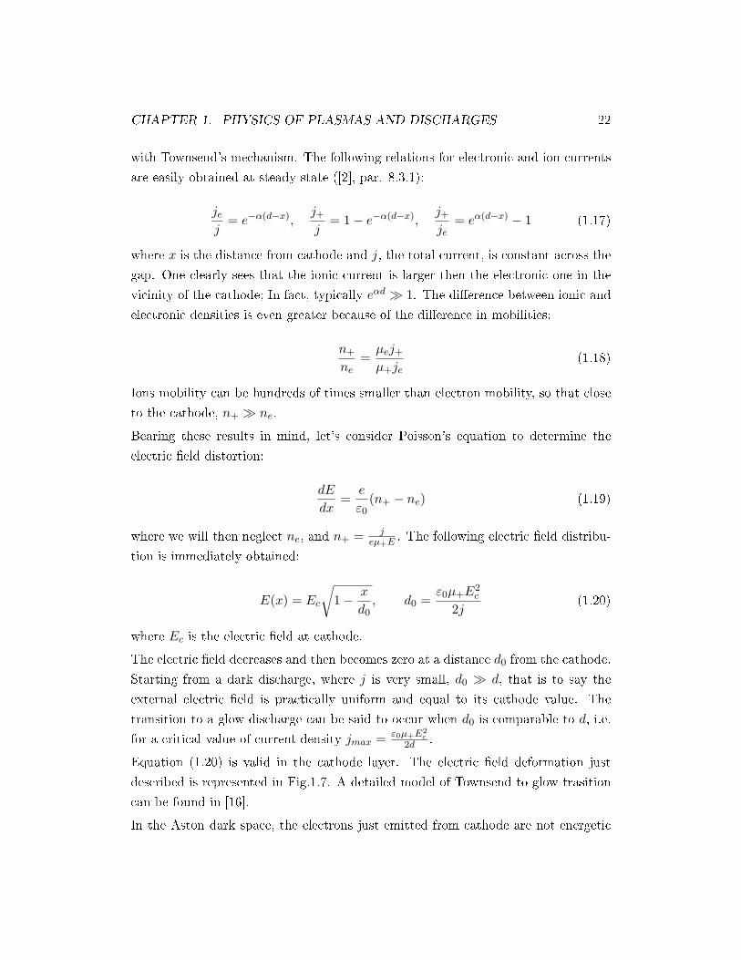
Bearing these results in mind, let's consider Poisson's equation to determine the
electric eld distortion:
dE
dx=
e
ε0(n+ − ne) (1.19)
where we will then neglect ne, and n+ = jeµ+E . The following electric eld distribu-
tion is immediately obtained:
E(x) = Ec
√1− x
d0, d0 =
ε0µ+E2c
2j(1.20)
where Ec is the electric eld at cathode.
The electric eld decreases and then becomes zero at a distance d0 from the cathode.
Starting from a dark discharge, where j is very small, d0 ≫ d, that is to say the
external electric eld is practically uniform and equal to its cathode value. The
transition to a glow discharge can be said to occur when d0 is comparable to d, i.e.
for a critical value of current density jmax = ε0µ+E2c
2d .
Equation (1.20) is valid in the cathode layer. The electric eld deformation just
described is represented in Fig.1.7. A detailed model of Townsend to glow trasition
can be found in [16].
In the Aston dark space, the electrons just emitted from cathode are not energetic

CHAPTER 1. PHYSICS OF PLASMAS AND DISCHARGES 23
Figure 1.7: Evolution of electric eld as current density increases in a dark to glow discharge
transition. Et is the breakdown eld. (Fridman, [3])
enough to cause electronic excitations or ionizations. In the next region, the cath-
ode glow, electronic excitations prevail, while in cathode dark space the avalanche
multiplication of charge takes place, and the discharge becomes self-sustaining. As
is apparent from Fig.1.6, electronic density reaches a maximum there, and the eld
its minimum: this is a clear evidence of nonlocal eects.
The positive column closes the electric circuit between the cathode layer and the an-
ode. The electric eld here is high enough to sustain the current and to compensate
the electrons and ions losses. At low pressures, electron losses are dominated by dif-
fusion, while at atmospheric pressure, bulk processes such as electron-ion dissociative
recombination become important.
What we have just described is the so-called normal glow regime (FG segment in
Fig.1.2). An important feature of this regime is its constant current density. When
current increases, then, the cross-section of the ionized channel grows until all the
anode area is occupied. At this point, the abnormal glow regime is entered, where
the current density increases and cathode emission intensies (GH segment). This
implies a cathode heating, until ionic impact emission is substituted by thermoionic
emission.
This new regime, where current can get as high as hundreds of A, is qualitatively
dierent from the previous, and is called arc regime. Apart from the cathode
emission mechanism, it is dierent also because it is formed by an equilibrium plasma.
Ions and neutrals, which usually remain at room temperature in glow and streamer
discharges, heat up considerably and reach electrons temperature.
Glow discharges are easily obtained and maintained in low-pressure conditions; at

CHAPTER 1. PHYSICS OF PLASMAS AND DISCHARGES 24
atmospheric-pressure, though, they tend to become unstable and constrict, giving
rise to a spark/arc transition. Thus, at atmospheric pressure, it is necessary to
use special geometries, electrodes, or excitation methods to obtain diuse glow dis-
charges.
1.2.3 Streamer mechanism
The Townsend mechanism denitely dominates at low values of p d (lower than 200
Torr·cm); at atmospheric pressure and centimeter size gaps, however, it could not
account for a number of phenomena, and a new theory was required to explain
extremely short-lived discharges. As experimental techniques improved, in fact, it
became clear that cathode secondary emission could not sustain the development of
such transient phenomena.
A new theory of electrical breakdown was thus developed by Meek [8], Loeb and
Raether in the 40's.
The fundamental idea is that if the external electric eld is high enough, the mul-
tiplication of charges in a primary avalanche is greatly enhanced by self-generated
electric elds, leading to the formation of a conducting channel between the two
electrodes. Let us now see the details.
The rst step, as in any breakdown process, is an electron avalanche. The propa-
gation of an avalanche initiated by a single electron near the cathode is illustrated
in Fig.1.8. The electrons move towards the anode with a drift velocity vd = µeE0,
where E0 is the applied electric eld. At the same time, the electron cloud spreads
by diusion around its central point x0 = vdt, r = 0, measured starting from the
cathode.
The radius of the propagating avalanche increases in time by the characteristic dif-
fusion law:
rD(t) =√
4Det =
√4Dex0µeE0
=
√8εmx03eE0
, (1.21)
where εm is the mean energy of electrons. This can be considered valid until charge
density is not too large.
As for the second step, we recall that the Townsend coecient, α, which regulates
charge multiplication, is a steep function of the electric eld. Therefore, if the latter

CHAPTER 1. PHYSICS OF PLASMAS AND DISCHARGES 25
Figure 1.8: Electron avalanche at two consecutive moments in time. E0 is the applied
electric eld. (Raizer, [2])
is large enough, the ionization process becomes so ecient that a considerable space
charge is produced. By considerable, we mean that its own electric eld (E′) is
comparable to the external one, and the two must be added up vectorially. This
means that a distortion of E0 takes place in the vicinity of the avalanche. This is
made clearer in Fig.1.9.
Figure 1.9: Field distortion in an avalanche to streamer transition. Left: E0 and E′ lines
shown separately. Right: resulting electric eld lines. (Fridman, [3])
From the gure, we see that the negative and positive centers of charge are separated;
this is because of electrons and ions dierent mobilities. Ions are in fact essentially
left behind by the negative front propagating towards the anode. This dipole
charge distribution causes the enhancement of electric eld at the head and tail of
the avalanche, and its reduction in the central region.

CHAPTER 1. PHYSICS OF PLASMAS AND DISCHARGES 26
Figure 1.10: Anode-directed (or negative) streamer with eld lines in the vicinity of the
head. (Raizer, [2])
The avalanche which propagates and grows by the mechanism just oulined, is the
precursor of the conducting channel, the actual streamer.
Two kinds of streamer are possible: cathode-directed (or positive) and anode-
directed (or negative) streamers. The former is initiated at the anode surface and
propagates towards the cathode. These streamers are sustained by photoionization1,
which causes secondary avalanches whose electrons move towards the positive head.
Our simulation model will not include photoionization, so we will not give further
details.
Anode-directed streamer can develop in suciently large gaps and/or at high over-
voltages. In this case, in fact, the avalanche transforms into a streamer before it
reaches the anode. This is portrayed in Fig.1.10.
The ionization front propagates at the expense of the electrons of the front, while
the electrons behind the front, moving in a weaker eld, do not separate from the
ions, forming a quasineutral plasma.
Streamer channels usually have diameters in the range 0.01-0.1 cm, and their growth
time-scale is of the order of tens of nanoseconds, i.e. they usually develop much
faster than the time necessary for ions to cross the gap and provide the secondary
emission. Furthermore, they usually branch in complicated ways, with dierent1Although this is still highly debated in the scientic community, even for the most basic aspects.
CHAPTER 1. PHYSICS OF PLASMAS AND DISCHARGES 27
branches getting at the electrode at slightly dierent times (see 1.2.4).
We now want to give a simplied criterion which can be used to roughly determine
whether a streamer is expected or not.
One necessary condition for avalanche-to-streamer transition is that the multiplica-
tion of charge carriers becomes so ecient that the electric eld of the avalanche is
comparable to the external one. Thus, if we assume that the charges of both signs
are within a sphere of radius R, the eld at its surface can be estimated as:
E′ =e
4πε0
eαx
R2(1.22)
where the leftmost e is the electron charge. Provided the amplication factor is
below 106, the diusion radius (1.21) can be used for R, but typical values can reach
the order of 108. In this case, Raizer suggests to use the inverse of the Townsend
coecient, i.e. R ∼ α−1, because the process is not diusion-dominated, but rather
Coulomb repulsion must be taken as the main source of the electronic cloud spread-
ing.
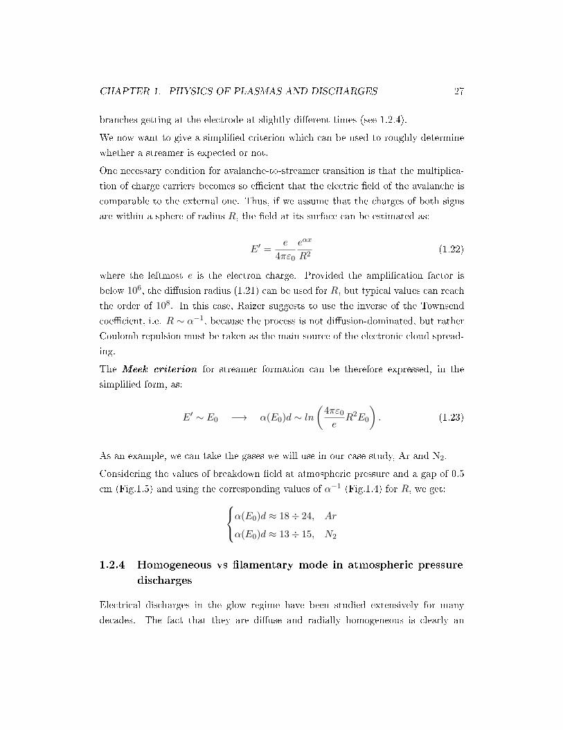
The Meek criterion for streamer formation can be therefore expressed, in the
simplied form, as:
E′ ∼ E0 −→ α(E0)d ∼ ln
(4πε0e
R2E0
). (1.23)
As an example, we can take the gases we will use in our case study, Ar and N2.
Considering the values of breakdown eld at atmospheric pressure and a gap of 0.5
cm (Fig.1.5) and using the corresponding values of α−1 (Fig.1.4) for R, we get:α(E0)d ≈ 18÷ 24, Ar
α(E0)d ≈ 13÷ 15, N2
1.2.4 Homogeneous vs lamentary mode in atmospheric pressure
discharges
Electrical discharges in the glow regime have been studied extensively for many
decades. The fact that they are diuse and radially homogeneous is clearly an

CHAPTER 1. PHYSICS OF PLASMAS AND DISCHARGES 28
advantage for homogeneous treatment of surfaces or deposition of thin lms. They
were (and still are, of course) tipically produced at low pressures (order of 1 mbar)
between two electrodes separated by gaps of few centimeters.
As anticipated in the previous paragraph, one of the rst issues with atmospheric
pressure discharges its their tendency to become unstable and constrict, in the sense
that a glow-to-arc transition easily occurs. A way to avoid the transition is to use one
or more layers of dielectric material between the electrodes. This kind of discharges
are known as dielectric barrier discharges (DBDs). They constitute our case
study. Basically, they prevent the transition to an arc by collecting charges on the
dielectric surfaces, thus generating an electric eld which gradually compensates the
external one; the discharge goes on until the breakdown condition isn't no longer
satised, and then it ceases. For this reason, DBDs must be powered in AC, or
through some pulsed voltage. Through the negative feedback mechanism we have
just outlined, an indenite growth of current density is prevented.
Traditional DBDs are generated by using alternating voltages with frequency in the
range 1-20 KHz. More recently, nanosecond-pulse DBDs have attracted wide interest.
In both cases, two regimes are possible, provided the arc regime is succesfully avoided:
homogenous and lamentary.
The rst mode, known in the literature as atmospheric-pressure glow discharge
(APGD), was rst described by Kanazawa [17]. It has several features in common
with the low-pressure analogue: for example, it is still a non-equilibrium discharge
(Te ≫ Ti,n), still works at the Stoletov point and is obviously sustained by secondary
emission at the cathode. Two dierences must be highlighted: in the atmospheric
pressure case, bulk loss processes are dominant (e.g., electron-ion ricombinative disso-
ciation), while at low pressure diusive processes are more important. Furthermore,
sheaths regions (see 1.3) are highly collisional, so that ions hit the electrodes with
much smaller energies.
The second mode, the lamentary discharge, is based on the streamer mechanism,
i.e. on the amplication of the electric eld on the ionization front of a propagating
avalanche. In this case discharges consist of thin ionized channels of diameters of
the order of 100 µm. In Fig.1.11, we present the visual dierence between the two
regimes, as reported in [12].
The two discharge modes can be distinguished through spectroscopic analysis, i.e.

CHAPTER 1. PHYSICS OF PLASMAS AND DISCHARGES 29
Figure 1.11: Homogeneous (a) vs lamentary mode (b) appereance in a parallel plate
dielectric barrier discharge, in N2. [12]
Figure 1.12: Voltage-current waveforms in homogeneous (c) and lamentary (d) mode in
a parallel plate dieletric barrier discharge in N2 (signal frequency: 20 KHz). [12]
by measuring the radiation they emit, but they can also be identied through the
current-voltage characteristic which is qualitatively dierent in the two cases, as
shown in Fig.1.12.
In the APGD case, for each semiperiod a single current peak is observed (lasting
about 10 µs), while in the lamentary mode one observes a series of short, intense
pulses which last about 20 ns each. Those closely spaced peaks are the result of
branches of the same streamer hitting the electrode at slightly dierent times, and
dierent streamers started at dierent places in the gap. It must be noted that,
in both cases, the homogeneous discharge or the series of microdischarges cease
when the maximum (or minimum) of the applied signal is reached, and they start
again after the polarity switches. This is due to the previously described charge
accumulation on the dielectric surfaces.
CHAPTER 1. PHYSICS OF PLASMAS AND DISCHARGES 30
In [12], the transition between the two regimes is studied with dielectric surfaces
covered by a polymer or alumina. In both cases the transition from glow to lamen-
tary mode is found to occur when the power dissipated in the discharge increases
(thresholds are found to be 3 and 10 W/cm3, respectively).
In [15], where an APGD is studied in a noble gas, He, it is shown that the homo-
geneous regime can be maintained until the breakdown is governed by Townsend's
mechanism, while the Meek criterion for the streamer formation isn't matched.
This situation is realized when enough seed electrons are homogeneously distributed
in the volume, to allow the formation of a number of small avalanches under low
electrical elds, inducing a progressive ionization of the gas and its Townsend break-
down, leading eventually to a glow discharge ([13]). This is conrmed also in the
case of a molecular gas as N2, where the discharge can be sustained in glow mode
provided a minimum density of metastable states (excited by impact) is reached.
They create seed electrons in the idle phase of the discharge, through Penning eect
([12]).
Recently, another version of DBDs has gained interest in the non-equilibrium plasma
community: nanosecond-pulsed DBDs. They are powered by applying a voltage
pulse with a width of tens of nanoseconds and repetition frequency varying from
single shot to 2 KHz. They have shown interesting behavior: researchers have found
that these discharges can reach higher current density [18], enhance discharge e-
ciency [19], and sustain higher density [20] than typical AC-powered DBDs. One of
their several applications consists in actuators for aerodynamic ow control. They
work almost always in the streamer regime, as found in [21].
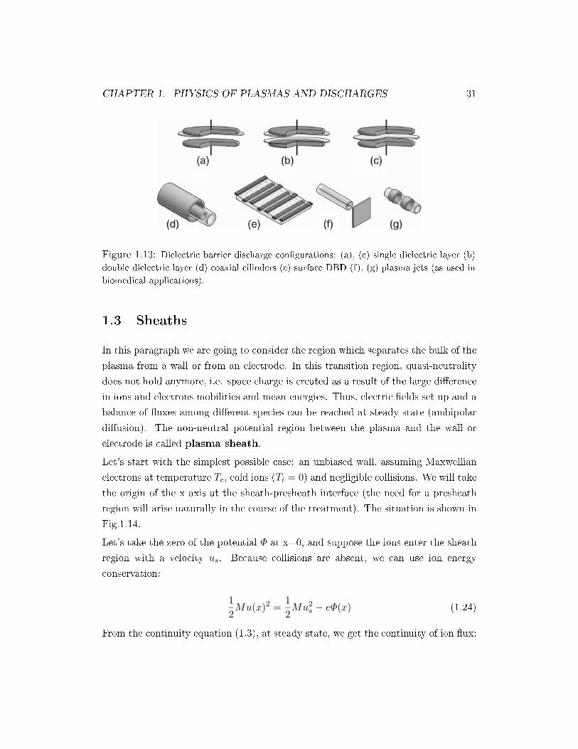
We show some of the most used congurations of DBD reactors in the following
gure.
CHAPTER 1. PHYSICS OF PLASMAS AND DISCHARGES 31
Figure 1.13: Dielectric barrier discharge congurations: (a), (c) single dielectric layer (b)
double dielectric layer (d) coaxial cilinders (e) surface DBD (f), (g) plasma jets (as used in
biomedical applications).
1.3 Sheaths
In this paragraph we are going to consider the region which separates the bulk of the
plasma from a wall or from an electrode. In this transition region, quasi-neutrality
does not hold anymore, i.e. space charge is created as a result of the large dierence
in ions and electrons mobilities and mean energies. Thus, electric elds set up and a
balance of uxes among dierent species can be reached at steady state (ambipolar
diusion). The non-neutral potential region between the plasma and the wall or
electrode is called plasma sheath.
Let's start with the simplest possible case: an unbiased wall, assuming Maxwellian
electrons at temperature Te, cold ions (Ti = 0) and negligible collisions. We will take
the origin of the x axis at the sheath-presheath interface (the need for a presheath
region will arise naturally in the course of the treatment). The situation is shown in
Fig.1.14.
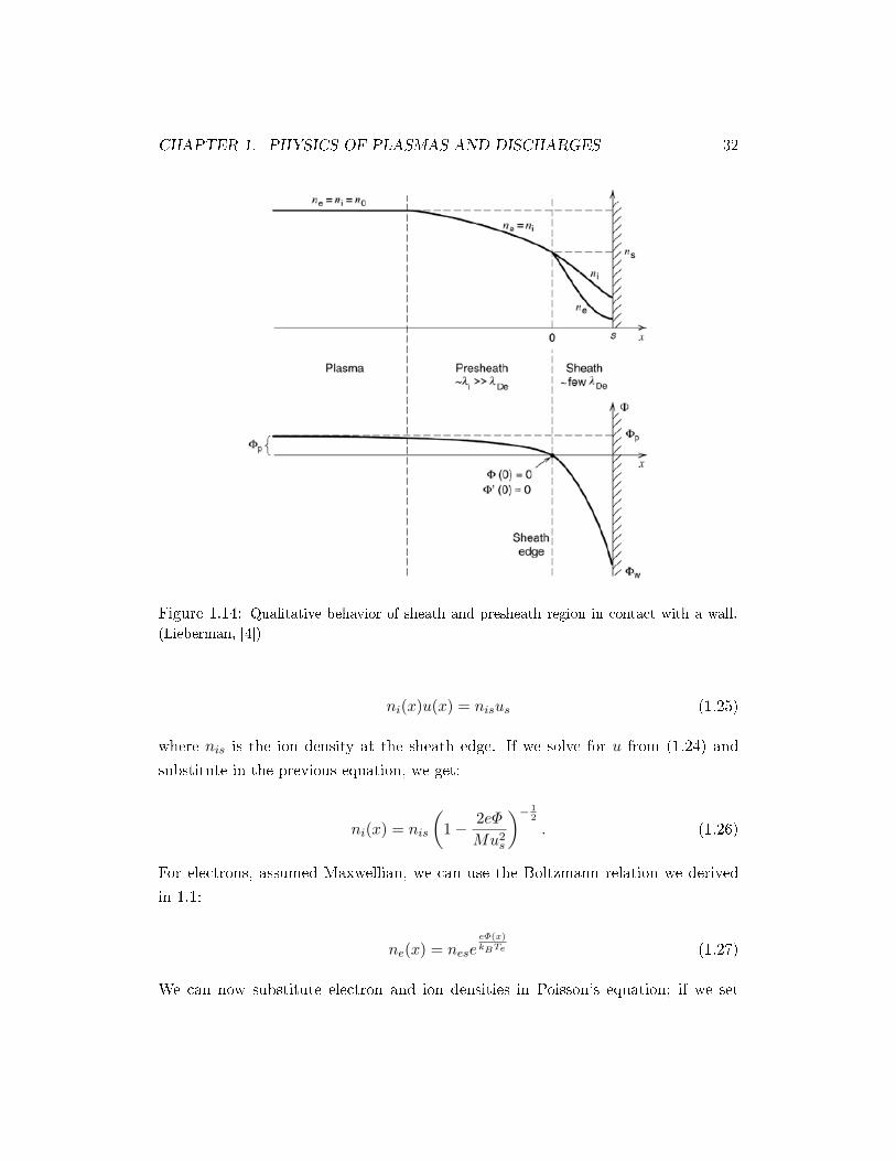
Let's take the zero of the potential Φ at x=0, and suppose the ions enter the sheath
region with a velocity us. Because collisions are absent, we can use ion energy
conservation:
1
2Mu(x)2 =
1
2Mu2s − eΦ(x) (1.24)
From the continuity equation (1.3), at steady state, we get the continuity of ion ux:
CHAPTER 1. PHYSICS OF PLASMAS AND DISCHARGES 32
Figure 1.14: Qualitative behavior of sheath and presheath region in contact with a wall.
(Lieberman, [4])
ni(x)u(x) = nisus (1.25)
where nis is the ion density at the sheath edge. If we solve for u from (1.24) and
substitute in the previous equation, we get:
ni(x) = nis
(1− 2eΦ
Mu2s
)− 12
. (1.26)
For electrons, assumed Maxwellian, we can use the Boltzmann relation we derived
in 1.1:
ne(x) = neseeΦ(x)kBTe (1.27)
We can now substitute electron and ion densities in Poisson's equation; if we set
CHAPTER 1. PHYSICS OF PLASMAS AND DISCHARGES 33
nis = nes ≡ ns at the sheath edge, we get:
d2Φ
dx2=
ens
ϵ0
[e
eΦkBTe −
(1− 2eΦ
Mu2s
)−1/2]
(1.28)
This is the fundamental nonlinear equation governing the sheath potential.
By manipulating it, it is easy to show that, for a solution to exist, us cannot assume
any value ; it must satisfy the so called Bohm sheath criterion:
us ≥ uB =
√kBTe
M, (1.29)
i.e. ions must enter the sheath with speeds at least equal to the ionic speed of sound,
known in this context as the Bohm velocity uB. The electric eld in the bulk of the
plasma is usually quite small, so a region with a suciently high potential drop must
develop in order to accelerate ions before they enter the sheath; this is called the
presheath region (see Fig.1.14).
We now want to estimate the potential drop in the sheath: we consider the ions and
electrons ux at the wall:
Γi = nsuB, (1.30)
Γe =1
4nsvee
eΦwkBTe , (1.31)
where Φw is the potential of the wall with respect to the sheath-presheath edge (x=0)
and ve = (8kBTe/πm)1/2 is the mean electron speed. Substituting for Bohm velocity
uB and setting the uxes equal to each other, we nally get:
Φw = −kBTe
eln
(M
2πm
) 12
. (1.32)
As expected, this potential is negative, i.e. electrons get conned in the bulk plasma
by an electric eld directed to the wall, while ions are accelerated towards it. The
potential drop is proportional to Te, with a factor dependent on the ratio of ions and
electrons masses. For Ar, for example, ln (M/2πm)12 = 4.8.
Undriven sheaths widths are typically a few Debye lengths.
CHAPTER 1. PHYSICS OF PLASMAS AND DISCHARGES 34
1.3.1 High voltage sheath
If the previously considered unbiased wall is substituted by a high-negative-voltage
driven electrode, i.e. the applied potential is much greater than Te, then the electron
density in the sheath is very small ne ∼ ns eeΦ
kBTe → 0. Thus, it is reasonable to make
the assumptions ne = 0, ni = ns; this is known as the matrix sheath.
Choosing x=0 at the sheath-plasma edge as before, and being s the sheath thickness,
we write:
dE
dx=
ens
ϵ0
which yelds a linear variation of the electric eld:
E =ens
ϵ0x
Integrating once again, we obtain a parabolic prole for the electrostatic potential:
Φ = −ens
2ϵ0x2
If we denote by −V0 the applied negative potential, i.e. Φ(s) = −V0, we get an
expression for the sheath thickness:
s =
√2ϵ0V0
ens(1.33)
or, in terms of the Debye length at the sheath edge:
s = λDs
√2V0
Te. (1.34)
We see that in this case the sheath width can be tens of Debye lengths.
In the steady state, the matrix sheath assumption is not consistent, because ions
accelerate during their motion and so their density cannot be constant. An expression
for ni(x) can be derived analogously to what we have done at the beginning of the
paragraph, by using ion energy and ux conservation, obtaining:

CHAPTER 1. PHYSICS OF PLASMAS AND DISCHARGES 35
ni(x) =J0e
(−2eΦ(x)
M
)−1/2
, (1.35)
where J0 is the constant ion ux. We use this in Poisson's equation:
d2Φ(x)
dx2= −J0
ϵ0
(−2eΦ(x)
M
)−1/2
. (1.36)
We multiply (1.36) by dΦ/dx and integrate from 0 to x, getting:
1
2
(dΦ
dx
)2
= 2J0ϵ0
(2e
M
)−1/2√−Φ (1.37)
with boundary conditions dΦ/dx = 0 at x=0. Taking the negative square root and
integrating again, we have
−Φ3/4 =3
2
(J0ϵ0
)1/2( 2e
M
)−1/4
x (1.38)
Finally, evaluating at x=s and solving for J0, we obtain the relation among the ion
current density, the applied voltage and the sheath thickness, a result sometimes
referred to as the Child-Langmuir law :
J0 =4
9ϵ0
(2e
M
)1/2 V3/20
s2(1.39)
All the previous results were obtained under the assumption of collisionless sheath;
at high pressure, however, collisions are very frequent, and the ion motion is mobility
dominated. If one supposes that ionization is negligible in the sheath, current con-
servation still holds, but the ion velocity must be expressed as µiE. Proceeding in
a similar fashion as in the previous case, Poisson's equation can be integrated twice
to give the collisional version of the Chil-Langmuir law:
J0 =
(2
3
)(5
3
)3/2
ϵ0
(2eλi
πM
)V
3/20
s5/2(1.40)
where λi is the ion mean free path.
However, high collisionality and a non-negligible ionization rate in the sheaths lead

CHAPTER 1. PHYSICS OF PLASMAS AND DISCHARGES 36
to very complicated analytical treatment, and no general solution is known. The
alternative, thus, is a kinetic numerical simulation, and the Particle-In-Cell (see
next chapter) method is one the most promising tool to investigate this region of the
discharge.
1.4 Non-equilibrium in low-temperature plasmas at at-
mospheric pressure
Low-temperature (or cold) plasmas are characterised by temperatures of the elec-
tron gas Te ≳ 1 eV , while ions and neutrals are often near room-temperature. One
of their most important feature is that they are often far from thermodynamic equi-
librium. In a context like this, the concept of temperature is almost never valid, and
will be used as an approximation.
The input source of energy in electrical discharges is the electric eld. Electrons
absorb energy more eectively because of their higher mobility. This energy is then
redistributed among the dierent degrees of freedom of the physical system: if the
rate of input is much smaller than the characteristic rates of redistribution through
collisions, we are in quasi-equilibrium conditions. Using high rates of energy input
and high rates of change increases the degree of non-equilibrium of the system; in
DBDs, this is achieved by applying nanosecond pulsed voltages or radio-frequency
signals.
The way light electrons transfer energy to heavy neutrals (atoms or molecules) is
strongly dependent on their kinetic energy. In atomic gases, for example, the energy
transfer from the electrons (for electron temperatures below 3 eV) to the heavy
particles is mainly due to elastic collisions, but this is highly inecient because
of the mass ratio of the particles involved (me/mg = O(10−5 ÷ 10−4)). In the
case of molecular gases, in the same range of energies, vibrational excitation can
be the dominant process. In any case, inelastic collisions (i.e. vibro-roto-electronic
excitation and ionization) have a threshold energy up to a couple of tens of eV.
A non-equilibrium plasma is of great interest, among other reasons, because it al-
lows in principle the selective production of reactive species (including electronic or
vibrational excited states, radicals, ions, photons), which can be in turn percursors
for desired chemical species. The latter can thus be obtained much more eciently

CHAPTER 1. PHYSICS OF PLASMAS AND DISCHARGES 37
than in thermal plasmas.
To x ideas, let's consider the following elementary process:
e+M(i) → e+M(f) (1.41)
where an electron excites a molecule from the initial state i to the nal state f. The
rate at which the nal state is produced starting from initial state is given by:
νif = Nikif = Ni
∫σif (v)vfp(v)dv [s−1] (1.42)
where Ni is the density of target particles in the initial state, kif is the reaction rate
coecient (i.e. the rate per unit density), σif (v) is the state-selective cross section
for the process at hand and fp(v) is the distribution function of the projectile. The
initial and nal state in the example can be any vibrational, rotational, electronic
level of the target species. Of course, analogous expressions are valid for all two-body
collisions: ionization, dissociation or recombination processes.
It's clear that the rate of the process is strongly dependent on the distribution of the
projectile (electrons in (1.41)), and thus the production of M(f) can be enhanced or
suppressed according to the distribution obtained in the discharge. In other words, if
one can nd working conditions such as the functional integral in (1.42) is maximized,
then the electron distribution function can be tailored for a specic application.
Under equilibrium conditions, the electron velocity distribution function (EVDF) is
the well known Maxwellian distribution at temperature Te:
fMaxw(v) =
(m
2πkBTe
) 32
exp
(− mv2
2kBTe
)(1.43)
while the corresponding electron energy distribution function (EEDF) is given by:
fMaxw(ε) = 2
√ε
π(kBTe)3exp
(− ε
kBTe
), (1.44)
which has units of eV −1. It is often convenient to consider the so called electron
energy probability function (EEPF), dened as f(ε)/√ε, with units of eV −3/2. In
the Maxwellian case, the EEPF is a straight line in a semi-log plot, whose slope is
inversely proportional to Te.

CHAPTER 1. PHYSICS OF PLASMAS AND DISCHARGES 38
In atmospheric pressure microdischarges, EEPFs are usually strongly time-modulated
and non-Maxwellian, despite the high collisionality (λ ∼ 0.1µm). This is clearly ev-
ident from [23] whose results are reported in Figure 1.15. Here, time evolution of
EEPFs in radio-frequency atmospheric-pressure microdischarges is shown along the
entire cycle for three dierent discharge gaps. A three-energy group distribution is
observed: low-energy electrons (ε <∼ 2 eV ) are trapped between the two oscillating
sheaths while the relatively weak electric eld of the bulk heat them ineciently;
midenergy electrons (2 eV < ε <∼ 20 eV ) result from the avalanches in the sheaths,
caused by high-energy electrons which are mainly secondaries produced at electrodes,
and accelerated in the sheaths. We can clearly see that mid- and high-energy elec-
trons do not last the whole rf cycle: the latter cause ionizations in the sheaths and
then rapidly lose their energy once they reach the bulk plasma, while the former are
also lost to the electrodes when the sheaths collapse.
Another example of deviation from Maxwellian behavior in atmospheric pres- sure
microdischarge is reported by a numerical model [20]. In Figure 1.16, the time
evolution of the EEDF is shown in the case of a nanosecond pulsed DBD in Ar. In the
initial stage of the discharge, i.e. during the rise time of the voltage pulse, the EEDF
is dominated by electrons with energy smaller than 15.76 eV, the ionization threshold
for Ar. As the applied voltage increases, more electrons with energy exceeding 15.76
eV turn up, but they are completely depleted after about 20 ns (during the plateau
of the applied voltage), because of collisions with neutrals.

CHAPTER 1. PHYSICS OF PLASMAS AND DISCHARGES 39
Figure 1.15: Time evolution of EEPF in a radio-frequency (13.56 MHz - 1 A/cm2)
atmospheric-pressure microdischarge in He, for three gap spacings. a) EEPF for electrons
in the whole gap. b) Space and time averaged EEPF. [23]
Figure 1.16: Time evolution of EEDF in a nanosecond-pulsed DBD in Ar (rise time 15 ns,
peak voltage 7 kV) [20]

Chapter 2
Kinetic Simulation of Electric
Discharges
2.1 Introduction
The study of low-temperature plasmas can be approached theoretically, experimen-
tally or through computer simulations. Diagnostic for microdischarges has only
recently made substantial progresses; in the past decades, the use of electrostatic
probes essentially developed for low-pressure (and thus relatively large-size) dis-
charges constituted a serious problem for microdischarge since they can heavily
perturb it and because the steep gradients obtained in such small systems require
remarkable time and space resolution. To circumvent these diculties, computer
simulation has always been a privileged tool, to which the plasma physics commu-
nity largely resort to identify research guidelines, nd optimum operating conditions
or propose novel designs for performance improvements. It goes without saying,
simulations acquire a growing importance as computer performances improve.
Simulating plasma dynamics may appear as a formidable task, if one looks at all the
processes that should be taken into account: solution of neutral and charged par-
ticle kinetics, radiation transport, Maxwell equations and large numbers of volume
and surface reactions. This should be done, obviously, in a self-consistent manner,
considering all the timescales shown in Fig. 2.1. In fact, incorporating all these
aspects in one detailed model would result in an untreatable and immeasurably
40

CHAPTER 2. KINETIC SIMULATION OF ELECTRIC DISCHARGES 41
Figure 2.1: Typical timescales of relevant processes in AP discharges. [22]
time-consuming simulation. So, one must consider simplied models and simula-
tion techniques, which can nonetheless be appropriate, if wisely chosen, to examine
particular problems.
After a brief overview of simulation methods, we will dive in the detailed description
of the Particle-In-Cell (PIC) - Monte Carlo Collision (MCC) method: this is the
simulation method on which our work is based. In the next chapter, we will de-
scribe the original code which has been written for the simulation of our case study:
nanosecond-pulsed DBDs.
2.2 Overview of simulation methods
The most used methods to simulate low-temperature plasmas are, in order of in-
creasing complexity:
1. State-to-state chemical kinetics models
2. Fluid models
3. Particle-based models
In the state-to-state chemical kinetics models, every excited state of atoms
or molecules is considered as an indipendent species. This leads to a system of
CHAPTER 2. KINETIC SIMULATION OF ELECTRIC DISCHARGES 42
master equations, which describe the temporal evolution of the population densities
of excited states under the action of collisional processes.
The kinetic equations for the i-th level population density (ni) in the case of an
atomic plasma can be written as:
dni
dt=
∑j>i
njAji + ne
∑j =i
njkji + n2en+kion + nen+βi
−ni
∑j<i
Aij − nine
∑j =i
kij − ninek3b ∀i (2.1)
while the electrons (ne) and ions (n+) densities come from the conservation equation:
dne
dt=
dn+
dt= −
∑i
dni
dt
where kij , kji, kion and k3b are the electron-impact rate coecient of excitation,
relaxation, ionization and three-body recombination processes, respectively. Aij is
the radiative transition probability and βi is the radiative recombination coecient.
The solution of the system of equations is based on the calculation of the dierent rate
coecients, where the EEDF often comes from a 2-term expansion approximation
of the Boltzmann equation. This method is by far the simplest and fastest.
We gave an introduction to the principles of uid models in 1.1. Fluid models
aim to describe the plasma dynamics by few quantities, namely plasma density,
mean velocity and mean energy. The equations for each of these quantities are
obtained, as shown, by taking velocity moments of the Boltzmann equation: they are
the continuity equation, the momentum transfer equation and the energy equation.
Maxwell equations (or Poisson's equation in the electrostatic case) must then be
coupled with uid equations to obtain self-consistent electromagnetic elds.
In the case of atmospheric pressure DBDs, where the momentum transfer collisional
frequency is usually larger than the radio-frequency driving frequency, the drift-
diusion (DD) approximation is often used. In this approximation, the charged
particles momentum equations are equivalent to, and thus substituted with, the
charged particles uxes written as the sum of a drift term and a diusion term. This
also implies that the inertia of the particles is assumed negligible.

CHAPTER 2. KINETIC SIMULATION OF ELECTRIC DISCHARGES 43
The following equations are a typical set which can be used to simulate a low-
temperature plasma in the electrostatic case [25]. The DD approximation is used
for electrons, while ions are considered massive and so the full ux equation is used
for them. In this example, ions are considered at the same temperature as the
background neutrals, so their energy balance equation is not solved.
Electrons:
∂ne∂t +∇ · Γe = Se (continuity)
Γe = −µeE −∇(Dene) (ux-DD)
∂(neεe)∂t +∇ ·
(53εeΓe − 2
3κ∇εe)= −eΓe ·E − neεcνiz (energy)
Ions:
∂ni∂t +∇ · Γi = Si (continuity)
∂Γi∂t + (ui · ∇)Γi =
ZieniMi
E − ∇(niTi)Mi
− νiNΓi (ux)
Field:
∇ · (ϵ∇ϕ) = −e(Zini − ne) (Poisson)
where e is the elementary charge, Zi the charge of ion species in units of e; Γe(= neue)
and Γi(= niui) the electron and ion uxes; ue and ui the electron and ion mean
velocities; Se and Si the source terms for electrons and ions resulting from colli-
sional processes; νiz and νeN the electron ionization and electron momentum transfer
rates; νiN the ion-neutral momentum transfer rate; εc(Te) the mean energy loss per
electron-ion pair created; εe(= 32Te) the mean electron energy; Te and Ti the electron
and ion temperatures in units of eV; µe(= e/meνeN ) and De(= Te/meνeN ) the elec-
tron mobility and diusion coecient; κ(= 52neDe) the scalar thermal conduction
coecient.
The above set of equations is not closed because the ionization and momentum
transfer rates cannot be expressed as functions of density, mean velocity and mean
energy. As we explained in 1.4, these rates must be expressed as averages over the
distribution function of the species at hand:
νif = Nikif = Ni
∫σif (v)vfp(v)dv (2.2)

CHAPTER 2. KINETIC SIMULATION OF ELECTRIC DISCHARGES 44
Therefore, one must choose fp(v) a priori, because the Boltzmann equation is not
solved. Of course, the simulation results will depend on the assumption. This
constitutes perhaps the main drawback of the uid approach to simulations, because
electrons (and other species as well) distributions can be very far from a Maxwellian,
which is commonly assumed as the energy distribution for each species (in this
case the frequencies and, as a consequence, the transport coecients are functions
of the particle mean energy, i.e. of the temperature). Other distributions (e.g.
Druyvesteyn) might also be considered.
One of the simplest alternative choices, however, is the local eld approximation
(LFA), which is based on the assumption that charged species gain energy from the
electric eld and lose this energy locally as a result of collisions. The LFA is then
valid when the following conditions are satised:
1
λm,E(z, t)≫ 1
E(z, t)∂zE(z, t),
νm,E(z, t) ≫1
E(z, t)∂tE(z, t),
where λm and νm are the mean-free-path and frequency for momentum trasfer, while
λE = λm
√νm/3νE and νE are the energy relaxation length and frequency.
Under this hypothesis the frequencies of the various elementary processes and the
transport coecients can be expressed as functions of the local reduced electric eld
E(x)/nN ; furthermore, the energy balance equation doesn't need to be solved. The
LFA fails in regions of strong eld gradients, in the case of high rates of change of the
applied eld or when non-local eects become important for the case under study.
The latter is often true in ns-pulsed atmospheric pressure microdischarges.
Despite their limitations, uid simulations are widely used to simulate plasmas in
a great variety of conditions, because of their advantage in computational speed,
which allows to treat without diculties 2D or even 3D cases. They are employed
very often to simulate complicated chemistry with lots of reactions involved.
Particle-based models are the most accurate among the possible choices, because
they are based on the numerical solution of the Boltzmann equation and so no
assumption about the distribution function is required; this aspect makes them the
ideal tool for studying the kinetics of the charged species. The particle-in-cell method

CHAPTER 2. KINETIC SIMULATION OF ELECTRIC DISCHARGES 45
will be explained in detail in the next paragraph.
2.3 The Particle-In-Cell method
The Particle-In-Cell (PIC) method is a powerful tool for the simulation of plasma
physics. Its introduction, due to the work of Buneman [27], Dawson [28], Hockney,
Birdsall, Morse and others, dates back to the end of the fties.
The basic idea on which the PIC method is based is rather simple, in principle:
charged particles are moved according to their equations of motion, and their posi-
tions and velocities are used as sources for the Maxwell equations which are solved
on an appropriate mesh. The elds are then interpolated to calculate the forces
acting on the particles.
The PIC method is also referred to as particle-mesh (PM), because the simulated
particles are converted into a set of density values on an appropriate mesh, thus al-
lowing the solution of the eld equations. This is the choice in plasma computational
physics; other possibilities are: particle-particle (PP) in which binary interactions
among particles are considered and PP-PM in which both types of interactions are
used. PP methods are not feasible in the case of plasmas because the computational
cost scales as N2 (N is the number of simulated particles) or at best as N log(N); it
is nonetheless widely used in molecular dynamics, where fewer particles need to be
simulated.
Let's introduce now the formal basis of the PIC in the context of plasma physics.
From the mathematical point of view our aim is to solve the Boltzmann equation
coupled with Maxwell equations:
∂fi(r,v,t)∂t = F fi(r,v, t) +Cfi(r,v, t)
1µ0∇×B = J + ε0
∂E∂t
∇×E = −∂B∂t
∇ ·E = ρε0
∇ ·B = 0
(2.3)
where i is the i-th charged species (electrons or ions); F and C are the collective
and collisional operator, respectively:
CHAPTER 2. KINETIC SIMULATION OF ELECTRIC DISCHARGES 46
F fi(r,v, t) = −v · ∂fi(r,v, t)∂r
− q
m(E + v ×B) · ∂fi(r,v, t)
∂v(2.4)
Cfi(r,v, t) =
(∂fi(r,v, t)
∂t
)coll
(2.5)
The coupling is accomplished through the source quantities, which are evaluated as
the rst two moments of the distribution functions:ρ =∑
i qi∫dvfi(r,v, t)
J =∑
i qi∫dv vfi(r,v, t)
If we consider time as discrete, Boltzmann equation becomes:
∆fi(r,v, t)
∆t= F fi(r,v, t) +Cfi(r,v, t) −→
fi(r,v, t+∆t) = [1 + (F +C)∆t] fi(r,v, t).
Neglecting second order terms, the previous can be written as:
fi(r,v, t+∆t) = (1 +C∆t)(1 + F∆t)fi(r,v, t),
and nally, splitting the collective and collisional part of the evolution, we get the
following recursive rule:f′i (r,v, t+∆t) = (1 + F∆t)fi(r,v, t)
f′′i (r,v, t+∆t) = (1 +C∆t)f
′i (r,v, t+∆t)
(2.6)
The rst of (2.6) corresponds to the evolution of the distribution function due to
volume forces (electromagnetic) while the second corresponds to the eect of col-
lisions. In this way, we have decoupled two dierent kinds of dynamics which can
be considered separately. Collisions will be treated in the next paragraph, in the
context of Monte Carlo collision method. For the present, we are going to focus on
the eect of the collective operator, introducing the concept of superparticle.
The fundamental assumption of the PIC method is that the distribution function

CHAPTER 2. KINETIC SIMULATION OF ELECTRIC DISCHARGES 47
of every charged species can be written as the superposition of several elements (we
drop the index i of the species):
f(r,v, t) =
N∑p=1
wpfp(r,v, t), (2.7)
where:
fp(r,v, t) = δ(v − vp(t))S(n)
(r − rp(t)
∆p
). (2.8)
The sum in (2.7) is the Klimontovich-Dupree discrete representation of the dis-
tribution function. It corresponds to a discretization of the phase space of the
species, which is divided into N small volumes called superparticles (or some-
times macroparticles). These little volumes in phase space are centered around the
position rp(t) and velocity vp(t), and each of them represents a bunch of wp phys-
ical particles, i.e. every macroparticle has an appropriate statistical weight. The
time evolution of macroparticle positions and velocities will give the solution to the
collisionless part of the Boltzmann equation.
The tensor product of (2.8) is the usual form for the distribution of a macroparticle,
although more general forms are sometimes used; δ is the Dirac delta distribution,
while S(n) is always chosen as a n-th order b-spline1, centered around rp(t), with ∆p
a xed parameter corresponding to the nite-size of the superparticle and related to
the cell size of the mesh used to solve Maxwell equations (discussed below).
In the context of the PIC method, S(n) are called shape functions of the macroparticle
and they are required to satisfy a number of properties:
1. Their support must be closed
1B-spline functions are piecewise polynomial functions. They can be obtained recursively start-
ing from the rst, at-top spline; in the one-dimensional case:
b0(x) =
1 |x| < 1/2
0 otherwise−→ bn(x) =
+∞w−∞
b0(x− x′)bn−1(x′)dx′

CHAPTER 2. KINETIC SIMULATION OF ELECTRIC DISCHARGES 48
2. Their integral is unitary:
+∞w−∞
S(n)
(r − rp∆p
)dr = 1
3. They are symmetric:
S(n)
(r − rp∆p
)= S(n)
(rp − r
∆p
)
B-splines satisfy all these requirements.
The next step consists in substituting (2.7) with (2.8) into the rst of (2.6), i.e. the
collective part of the Boltzmann evolution. The result is ([30], [32]):
f ′p
(rp + vp∆t,vp +
qpmp
(E + vp ×B)∆t, t+∆t
)= fp(rp,vp, t), (2.9)
for each of the N macroparticles, with qp = qwp and mp = mwp their charge and
mass, respectively.
This is a fundamental result: it states that the p-th macroparticle's distribution
function doesn't change along a trajectory given by the classical Newton equation
with the Lorentz force:
drp
dt = vp
mpdvp
dt = qp(E + vp ×B)(2.10)
We can thus solve the collisionless part of BE (which can in fact be written, using the
comoving derivative, as df/dt = 0), by simply following every macroparticle along
its trajectory, determined by the self-consistent electromagnetic eld. In this way,
we have formally justied the reasonable idea that our plasma can be simulated by
moving a certain large number of charged particles. It must be noted that the charge
to mass ratio is the same for the physical and computational particles, so that they
move along the same trajectories: qp/mp = q/m.
There is, however, an aspect we have just touched lightly, that is to say the nite
size of the superparticles which has emerged in (2.8), through the parameter ∆p. We
want to elaborate a bit on this now; what follows is the line of reasoning used by

CHAPTER 2. KINETIC SIMULATION OF ELECTRIC DISCHARGES 49
Figure 2.2: Force law between nite-size spherical particles in 2D for various particles size
(assuming gaussian-shaped charge-density prole) [29].
Dawson [29].
We know that the force between two charged point particles becomes very large as
they approach. On the other hand, the slow fallo of the Coulomb force with distance
gives rise to collective eect which we have considered in Chapter 1 and which we
surely want to retain in the computer simulation. If we replace point particles with
nite-size particles which are free to pass through each other, their interaction with
distance is modied as shown in Fig. 2.2.
We see that as the distance increases and becomes eventually greater than their size,
the interaction is the same as the Coulomb force between point particles, but when
the superparticles overlap the inteaction goes to zero. The use of nite-size particles
thus allows to correctly describe the collective behavior which is a characteristic
feature of plasmas, but the rapidly varying forces associated with close encounters
are greatly reduced.
That this last eect is advantageous for our purposes, can be understood by intro-
ducing the plasma coupling parameter, dened essentially as the ratio of the

CHAPTER 2. KINETIC SIMULATION OF ELECTRIC DISCHARGES 50
thermal (i.e. mean kinetic) and mean potential energy of the particles:
Λ =kBT
q2/4πϵ0d(2.11)
where d is the mean interparticle distance. The system is said to be strongly coupled
if Λ ≪ 1, because in this case the trajectories are strongly aected by near neighbour
interactions (Coulomb collisions are important); the converse is true if Λ ≫ 1, and
the plasma is weakly coupled.
Finite-size particles, as we have just seen, are characterised by a reduced potential
energy, for the same kinetic energy. The consequence of this situation is that the
same plasma coupling parameter as the real plasma is reached with fewer particles,
a very useful eect from the computational point of view.
The size of the superparticles, which appears in the tensor product of fp as ∆p,
must clearly be related to the length scales that we wish to resolve. We know
from Chapter 1 that the fundamental length scale in plasmas is the Debye length,
λD; it represents the typical distance over which charges or elds are shielded in
the plasma and, accordingly, over which there can be remarkable deviations from
the macroscopic neutrality of the system. We certainly want to faithfully simulate
what happens on this natural scale, but at the same time we cannot resolve density
variations over regions smaller than the size of the macroparticles, because they are,
so to speak, "rigid" objects. These two facts dictate the following constraint:
∆p ≲ λD. (2.12)
For the same reasons, in making calculations, we may divide the space into cells
which are about the size of the particles (∆x ∼ ∆p), because the dynamics on smaller
scales is not realistically simulated. This reasoning has so led us quite naturally to
the introduction of amesh, which will be used for the solution of the eld equations:
the idea is to solve them on this computational grid. We are thus faced with the
problem of discretizing these equations.
The number of physical particles which make up a superparticle, wp, has to be large
enough so that a reasonable number of superparticles is simulated; at the same time,
it has to be small enough so that the number of particles per cell is statistically
signicant.

CHAPTER 2. KINETIC SIMULATION OF ELECTRIC DISCHARGES 51
Figure 2.3: General scheme of a PIC simulation
We have presented here the main basic ideas and motivations behind the PIC
method. We must now ll the gap between the equations derived and the self-
consistent solution of our problem through a computer. We will do this in the next
paragraphs. The logical order of the PIC routine is represented in the Figure 2.3.
2.3.1 The particle mover
As in all numerical codes, time (as well as space) must be discretized in order to
turn dierential equations into algebraic equations; let's denote by ∆t the chosen
time step, and by Ak the value of the physical quantity A at time tk = t0 + k∆t,
with k an integer.
Positions and velocities must be updated according to the equation of motion EOM
(2.10); a widely used discretized form of the equations of motion is given by the
leap-frog scheme :
rk+1 − rk∆t
= vk+1/2 (2.13)
vk+1/2 − vk−1/2
∆t=
qpmp
(Ek +
vk+1/2 + vk−1/2
2×Bk
). (2.14)
Positions and velocities are not evaluated at the same time step, in fact velocities

CHAPTER 2. KINETIC SIMULATION OF ELECTRIC DISCHARGES 52
Figure 2.4: Leap-frog scheme update of position and velocity. [30]
are updated at tk+1/2 instead of tk+1; this allows to write time-centered equations.
Moreover, leap-frog is an explicit solver, i.e. velocities are updated using forces from
the previous time step. The leap-frog scheme is illustrated in Figure (2.4).
Time integration schemes of EOM must satisfy a series of criteria in order to guaran-
tee that the nite-dierence approximation of the continuous equations makes sense.
They can be grouped in the following way (Hockney-Eastwood, [30]):
• Consistency
• Accuracy
• Stability
• Eciency
Consistency requires that the chosen discrete equation tends to the respective
dierential equation as ∆t → 0. That this is true for the leap-frog scheme can be
easily shown by a Taylor expansion of the advanced positions and velocities around
their old values. Another consistency requirement is that symmetry under time-
reversal is maintained: time-centered equations are employed (also) for this reason.2
A time scheme satises the requirement of accuracy if the dierence between the
computed values and the solution of the dierential equation decreases as the time
step decreases, as we intuitively expect. To be more precise, the order of a time
integration scheme is p if the error scales, in a time step, as ∆tp. Thus, accuracy2Sometimes, time-centered equations lead to implicit schemes, using forces evaluated at the new
time step; this in turn leads to equations which must be inverted. The computational cost of
inversion cannot usually be aorded, and so explicit schemes which are not time-centered are used.
CHAPTER 2. KINETIC SIMULATION OF ELECTRIC DISCHARGES 53
has to do with local errors, essentially due to roundo and truncation. The order of
the leap-frog scheme is now derived.
Let's combine the two equations of the scheme, eliminating velocity and obtaining:
rk+1 − 2rk + rk−1
∆t2=
F k
mp, (2.15)
where F k is the force at time k. If we callR the solution to the continuous dierential
equation of motion (d2R/dt2 = F /m), and we substitute it in the previous, we can
write:
Rk+1 − 2Rk +Rk−1
∆t2=
F k
mp− δk, (2.16)
where δk is the truncation error at time k. By a Taylor expansion of Rk+1 and Rk−1
around Rk, we get:
d2R
dt2+
∆t2
12
d4R
dt4+ o(∆t2) =
F k
mp− δk, (2.17)
from which we get δk ∼ ∆t2, i.e. the leapfrog is second-order accurate. The general
requirement is that p > 1.
Stability is a global requirement: a time integration scheme is said to be stable if
local errors do not grow with time, i.e. a small error at any time step does not lead
to a larger error later on.
In order to determine whether a scheme is stable or not, one has to nd the equation
for the time evolution of errors and analyze its solutions. We will give a trace of the
ideas involved for the leapfrog method (for notational simplicity, we consider the one
dimensional case).
We dene the error in the position at time step k as:
ϵk ≡ xk −Xk. (2.18)
After some mathematical handlings, the following evolution equation is obtained
[30]:

CHAPTER 2. KINETIC SIMULATION OF ELECTRIC DISCHARGES 54
ϵk+1 − 2ϵk + ϵk−1 = − 1
m
∣∣∣∣ ∂F∂xp∣∣∣∣max
∆t2ϵk
= −Ω2∆t2ϵk, (2.19)
where an oscillatory solution has been assumed. In this case, the solutions will be of
the form ϵk = λk ∼ exp(iωn∆t), where λk is the k-th power of λ. We then substitute
this solution in the previous and we divide by λk−1, obtaining the characteristic
equation:
λ2 − 2λ+ 1 = − (Ω∆t)2 λ (2.20)
It has two solutions, λ±(Ω∆t). The general solution of (2.19) can be written as:
ϵk = αλk+ + βλk
− (2.21)
where all the quantities on the rhs may be complex.
We now clearly see that the propagation of errors depends on the solutions of the
characteristic equation; more precisely, the amplitude of the error depend on the
modulus of λ±.
An integration scheme can thus be said to be stable if the characteristic solutions
of the error evolution equation both lie within or on the unit circle in the complex
plane (|λ| ≤ 1).
In order to understand how the stability is aected by the choice of the parameter ∆t
on which λ± depend, one can analyze how these solutions move across the complex
plane as ∆t is increased from zero to innity. When any root cross the unit circle,
the scheme becomes unstable. This gives a constraint on the choice of timestep. In
the case of the leapfrog, the analysis gives the following limit for the stability of the
scheme:
∆t <2
ωp,
where ωp is the electron plasma frequency. Very often, a more restrictive condition
is used:

CHAPTER 2. KINETIC SIMULATION OF ELECTRIC DISCHARGES 55
∆t ≤ 0.2
ωp(2.22)
in order to get more accurate results.
This constraint on the timestep is not surprising: the reciprocal of the plasma fre-
quency gives the typical timescale of the response of our system to external pertur-
bations. We certainly want to resolve these eects and so ∆t < ω−1p is a reasonable
assumption in the rst place.
Two other restrictions on the choice of timestep are:
a) ∆t ≤ 0.1νcoll
, where νcoll is the total electron-neutral collision frequency. This is
necessary in order to faithfully represent the eect of collisions in the MCC.
b) the Courant-Friedrich-Levy (CFL) stability condition: ∆t ≤ ∆xvd
, where vd is the
electron drift velocity µeEx, and ∆x is the cell size. In other words, a superparticle
must not cross the boundary of a cell in a timestep. This is a general result for the
stability of the numerical solution of a dierential equation [31].
Eciency requires to use memory and time in the best possible way, provided the
constraints due to accuracy and stability are satised. Of course, eciency and ac-
curacy are usually competitive factors, and a compromise is in demand. In practice,
very often the best compromise is reached by using time integration schemes which
are second-order accurate (e.g. leapfrog) and adjusting the timestep accordingly.
2.3.2 Particle and eld weighting
Plasma governing equations are non-linear and they give rise to self-consistent struc-
tures: superparticles must be moved according to electric and magnetic elds whose
sources are the densities and currents of the superparticles themselves; these elds
superimpose to externally applied ones. Therefore, at every timestep, the elds must
be updated as well, solving the appropriate Maxwell equations on a computational
mesh. The problem then arises of assigning suitable values for the densities and
currents to the mesh points. This process, which we now describe, is called particle
weighting.
The case treated in the present thesis is electrostatic. Therefore, the Maxwell system
reduces to Poisson's equation:
CHAPTER 2. KINETIC SIMULATION OF ELECTRIC DISCHARGES 56
∇2φ = −ρ(r)
ε0. (2.23)
Furthermore, we will consider a one-dimensional system. Our problem is to establish
a procedure to assign a value to ρ(xk) ≡ ρk (where xk is the centre of the k-th cell of a
1D mesh with constant spacing∆x), starting from the positions of the superparticles.
The most straightforward approach is starting from the average charge density cen-
tered at xk:
ρ(xk) =1
∆x
∫ xk+1/2
xk−1/2
ρ(x)dx, (2.24)
where xk±1/2 are the cell vertices, which are ∆x/2 distant from xk. The previous
expression can be written, remembering the denition of the zero-th order spline, as:
ρ(xk) =1
∆x
∫ +∞
−∞b0
(x− xk∆x
)ρ(x)dx. (2.25)
We now recall the expression of ρ(x) (we assume there's only one charged species for
notational simplicity but the generalization is trivial):
ρ(x) = q
∫f(x, v, t)dv =
N∑p=1
qwp
∫fp(x, v, t)dv
=
N∑p=1
qwp
∫δ(v − vp)S
(n)
(x− xp∆p
)dv =
N∑p=1
qwpS(n)
(x− xp∆p
), (2.26)
where we have used the Klimontovich representation (2.7) and (2.8). Substituting
in (2.25), we obtain:
ρ(xk) =
∑Np=1 qp
∆x
∫ +∞
−∞b0
(x− xk∆x
)S(n)
(x− xp∆p
)dx, (2.27)
with qp the charge of the macroparticle.
We dene the weighting function as:
W (xk − xp) ≡∫ +∞
−∞b0
(x− xk∆x
)S(n)
(x− xp∆p
)dx (2.28)

CHAPTER 2. KINETIC SIMULATION OF ELECTRIC DISCHARGES 57
Figure 2.5: Weighting functions for the NGP and CIC schemes (1D). [33]
so that the nal expression for the charge density at mesh point xk is:
ρ(xk) =1
∆x
N∑p=1
qpW (xk − xp). (2.29)
The role of the weighting function is fundamental: it gives the contribution of a
macroparticle whose center is at xp, to the charge density at xk. A particularly
simple case occurs if the particle size and grid spacing are assumed equal (∆p = ∆x);
in fact, recalling the recursive denition of the b-spline (see footnote at page 47), in
this hypothesis we can write:
W (xk − xp) = bn+1
(xk − xp∆x
)The higher the order of the splines, the more accurate the weighting scheme. On the
other hand, the cost of using high-order splines aects heavily the execution time
of the simulation, because weighting must be performed at each timestep, for every
particle. In practice, in the great majority of cases, the two schemes are used: zero or
rst-order weighting schemes, known respectively as nearest-grid-point (NGP) and
cloud-in-cell (CIC). The weighting functions for these cases are shown in Figure 2.5.
The NGP scheme assigns every macroparticle to its nearest neighbor in the mesh,
with weight equal to one; the CIC, instead, uses the two nearest neighbors, assigning
to each of them a weight which is proportional to the distance of the centre of the
macroparticle from them, hence its alternative name, linear weighting. The latter is
more accurate and more often used than the NGP because it gives smoother forces,
and avoids more eciently the articial heating of electrons which can occur because
of the discontinuous variation of ρ as the superparticles cross cell boundaries (see
[30], chapter 5).

CHAPTER 2. KINETIC SIMULATION OF ELECTRIC DISCHARGES 58
The weighting function for the CIC, which is our choice in the simulation, is:
W (xk − xp) =
1− |xk−xp|∆x |xk − xp| ≤ ∆x
0 otherwise. (2.30)
Once Poisson's equation has been solved (see next section), we have at our disposal
the potential calculated at mesh points. The electric eld is then determined by the
space-centered equation:
Ek = −φk+1 − φk−1
2∆x. (2.31)
Particles move in a continuum, so we need to interpolate the elds from mesh points
to particle locations. This problem is called eld weighting. In order to assure
momentum conservation, eld and particle weighting are choosen to use the same
weighting function, so that:
E(x) =∑k
E(xk)W (x− xk) (2.32)
where the sum is over the grid points.
For completeness, we stress that another condition is necessary for momentum con-
servation, namely that the eld solver has the proper space symmetry, so that the
eld can be expressed as E(xk) =∑
i gkiρ(xi), with gki = −gik. In this way, it can
be shown that action-reaction law is valid, and self-forces are zero [33].
2.3.3 The eld solver
Particle weighting determines the source of Poisson's equation, i.e. charge density,
on each grid point. The methods used to solve the eld equation belong, in general,
to dierent classes and there is not a method which is the best a priori. A broad
classication is the following:
• Mesh-relaxation methods: the solution is at rst guessed on the grid, and
then relaxed to the nal solution, with the desired accuracy;
• Matrix methods: in this case the dierential equations are approximated

CHAPTER 2. KINETIC SIMULATION OF ELECTRIC DISCHARGES 59
as a system of linear nite-dierence equations and solved by some matrix
method;
• Rapid elliptic solvers: they use special techniques based on Fast Fourier
Transform and cyclic reduction.
Crucial discriminating factors are whether the equation is linear or not, and the
separability of the operator which acts on the eld. The nature of the boundary
conditions may play an important role, as well.
In the case of interest, i.e. 1D-cartesian electrostatic, the laplacian operator can be
discretized as:
∂2φ
∂x2−→ akφk+1 + bkφk + ckφk−1
∆x2. (2.33)
The system of linear equations have the following form:
akφk+1 + bkφk + ckφk−1 = dk k = 1, ..., Ng (2.34)
where Ng is the number of grid points and dk represents the charge density source.
For the solution of this set of equations we have choosen the Thomas Tridiagonal
Algorithm, which belongs to the class of matrix methods. It is based on two
iterative steps:
• Forward elimination:
ω1 =c1b1, ωi =
cibi − aiωi−1
i = 2, 3, ..., Ng − 1
g1 =d1b1
, gi =di − aigi−1
bi − aiωi−1i = 2, 3, ..., Ng
• Backward substitution:
φNg = gNg , φi = gi − ωiφi+1 i = Ng − 1, ..., 2, 1.
We now want to determine the coecients a, b and c, requiring second-order accuracy
for our scheme. So, we return to (2.33).
CHAPTER 2. KINETIC SIMULATION OF ELECTRIC DISCHARGES 60
The coecients are in our case constant, i.e. they do not vary sweeping the grid.
From symmetry we have a = c. By Taylor expanding around φk, we obtain:
φk±1 = φk +∆xφ′k +
∆x2
2φ
′′k ±
∆x3
6φ
′′′k +
∆x4
24φ(4)k + ... (2.35)
so that:
aφk+1 + bφk + cφk−1 = φk(2a+ b) + φ′′ka∆x2 + φ
(4)k a
∆x4
12+ ... (2.36)
If one then chooses a = c = 1 and b = −2, the dierence between the continuous
and discretized derivative becomes:
∂2φ
∂x2− φk+1 − 2φk + φk−1
∆x2= φ
(4)k
∆x2
12+O(∆x4), (2.37)
i.e. a second-order accuracy.
2.4 The Monte Carlo Collision method
Up to now, we have described how to move the superparticles in a self-consisted
eld, thus solving the collisionless part of the Boltzmann equation (known also as
Vlasov equation), i.e. the rst of (2.6). We must now devise a treatment for the
collisions, so that also the second of those equations is solved.
In a plasma, lots of types of collisions can take place; in our case study, because of
the weak ionization of the plasma, Coulomb collisions will be neglected, i.e. only
electron-neutral, ion-neutral collisions and, in the molecular gas case, electron-ion
recombination processes will be considered. Therefore, we will give here the ele-
mentary basis of the stochastic treatment of collisions involving charged and neutral
species; further details which apply to our specic simulation hypoteses and complete
these general considerations will be given in the Chapter 3 on code analysis.
Collisions between a charged particle, say an electron, and a neutral particle can be
treated basically by: a) Direct Monte Carlo Collision (DMC) and b) Null-Collision
Method.

CHAPTER 2. KINETIC SIMULATION OF ELECTRIC DISCHARGES 61
Direct Monte Carlo Collision
In this method, the time between two successive collisions is considered as a random
variable whose distribution is:
P (t) = 1− e−νt. (2.38)
Here, ν is the total collision frequency, i.e. the sum over all possible elementary
processes considered in the specic simulation model, ν =∑
i νi, while the i-th
collision frequency is given by:
νi = nNg σi(g),
where nN is the local density of neutrals (in general, of the target particles), σi(g) the
total cross section of the i-th process and g = |v − V | the relative speed of colliding
particles; if the target particle is much heavier than the incident one, very often the
cold target approximation is used: g = v, i.e. the information on target motion is
completely discarded. The collision frequency for a given process is dependent on a
local quantity, the target density, and basically the energy of the projectile.
The DMC is based on the sampling of the free ight time from the distribution
function (2.38). In general, if f(x) is the normalized distribution of the random
variable x with values in the range [0,+∞], then the sampling of the distribution is
accomplished by generating a set of numbers Rj uniformly distributed in the [0, 1]
range, and then solving for yj in the expression Rj =∫ yj0 f(x)dx. In other words, yj
can be shown to be distributed according to f(x).
In the case of (2.38), the time after which a particle collides is given by:
tcoll = − lnR
ν; (2.39)
this means that a counter must be used: it is given the zero value just after the
previous collision and is incremented at each timestep until tcoll > k∆t, where k is
an integer. When tcoll ≤ k∆t, the particle undergoes a collision.
If we suppose that m elementary processes are included in the model for the species
at hand, the rst type of collision is picked if

CHAPTER 2. KINETIC SIMULATION OF ELECTRIC DISCHARGES 62
r ≤ P1(tcoll)
P (tcoll)=
1− e−ν1tcoll
P (tcoll),
where r is a uniformly distributed random number; otherwise the second type is
picked if
P1(tcoll)
P (tcoll)< r ≤ P1(tcoll) + P2(tcoll)
P (tcoll)
and so on until r falls in the right interval.
We stress that, in general, ν∆t ≪ 1, i.e. on the average the particle collides after
lots of timesteps have elapsed (recall the constraint a explained at page 55).
Null Collision method
In the DMC, all particles have to be analyzed and followed until a collision occurs.
A more eective alternative is the Null Collision method. It exploits the fact that
collisions among charged particles and neutrals are relatively rare events, i.e. at each
timestep only a small part of the particles collides. Therefore, one can estimate the
maximum probability for such an event to occur in a timestep of the PIC:
Pmax = 1− e−νmax∆t
This represents the fraction of charged particles which are analyzed per timestep, i.e.
Nnc = PmaxN ≪ N . The procedure is much more ecient because a much smaller
number of particles is considered and no time counter is required.
Once this number is determined, the procedure is identical to the DMC, except for
the fact that the colliding particles are choosen by uniformly sweeping the charged
particles population:
j = RiN, i = 1, ..., Nnc
where Ri is uniformly distributed in [0, 1].

CHAPTER 2. KINETIC SIMULATION OF ELECTRIC DISCHARGES 63
Determining post-collision velocities
Once a particle collides with a neutral, its post-collision velocity must be determined.
From a formal point of view, this information comes as part of the solution of the
collisional part of the Boltzmann equation, the second of (2.6). Following Nanbu
[34], the probability density function of the p-th particle at time t+∆t has the form:
f ′′p (v, t+∆t) = (1− Pp)δ
(3)(v − vp) + PpQp(v) (2.40)
where Pp is the probability for a collision to occur; we have just treated this part
of the evolution. We will instead focus on the Qp term and its meaning; it can be
written as:
Qp(v) =
Nn∑q=1
Ppq
PpQpq(v) (2.41)
Here, Nn is the number of neutrals in the cell where the incident particle is located,
Ppq/Pp is the conditional probability that the collision partner of the particle is the
q-th neutral if a collision occurs in ∆t, and Qpq(v) is the probability density function
for the post-collision velocity. Its expression is the following:
Qpq(v) =σdiff (gqp, θ, ϕ)
σ(gqp)sinθ dθ dϕ δ(
∣∣g′qp
∣∣− gqp)dg′qp, (2.42)
where the rst term is the ratio of dierential and total cross section, gqp = vp−V q
is the relative velocity of particle and target before the collision. Through this
relation, the magnitude and direction of g′qp can be determined, and eventually the
post-collision velocity of the projectile is evaluated as:
v =1
mp +Mq(mpvp +MqV q +Mqg
′qp) (2.43)
Depending on the specic case, the target post-collision velocity update may be dis-
regarded, the selection phase of the collision partner may be skipped and, especially
for electrons, the gas initial velocity may be neglected.
What we have just described are the general principles on which collisions treatment
is based. As anticipated, we will give the explicit details of the procedure used in

CHAPTER 2. KINETIC SIMULATION OF ELECTRIC DISCHARGES 64
our case in the next chapter, where we are going to consider the particular features
of the code developed for the case studies.
Chapter 3
Description of the PIC-MCC
model developed
In this chapter we will describe the main features of the code developed at CNR-
NANOTEC of Bari implemented to simulate ns-pulsed driven dielectric barrier dis-
charge at atmospheric pressure.
3.1 Physical system and numerical parameters
The model developed consists in a fully kinetic PIC-MCC simulation,that is to say
each charged species is represented by macroparticles with equal weight and moved
according to Newton's equation. Neutrals are not followed during their motion.
The simulation is 1D-3V electrostatic: all particles are moved in one spatial di-
mension (normal to the electrodes) while all the three components of their velocities
are updated. Poisson's equation is solved in one dimension to evaluate the electric
potential φ(z).
From a physical point of view, the one-dimensional assumption corresponds to the
hypothesis that the transport along transversal (normal to z) directions is much
slower than the one along the z axis (see Figure 3.1).
Because we are 'neglecting' two spatial dimensions, the charge of every macroparticle
q has units of C/m2 and we cannot evaluate currents, but only current densities.
65

CHAPTER 3. DESCRIPTION OF THE PIC-MCC MODEL DEVELOPED 66
The discharge is ignited between two electrodes separated by a distance L of 1 cm,
by applying a high-voltage negative pulse (HVNP) of trapezoidal shape to one of
them, while the other is covered with a 0.5 cm thick dielectric layer (ϵ = 3.5ϵ0) and
grounded. This kind of electrical discharges are known as capacitive dielectric-
barrier microdischarges.
The geometry and the shape of the applied voltage (with some typical values) are
illustrated in Figure 3.1. The gap is the region comprised between the dielectric
surface, at zd, and the rightmost electrode: it is therefore 0.5 cm wide in our case
(i.e. L− zd).
Figure 3.1: Geometry with boundary conditions of our case study (top);
Voltage applied to the biased electrode (bottom)
Poisson's equation ∇ · (ϵ(r)∇φ(r)) = −ρ(r) is solved in 1D with the following
boundary conditions:
1. φ(0) = 0 (grounded electrode)
2. ϵ0∂φ(z→z−d )
∂z − ϵ∂φ(z→z+d )
∂z = σ(zd) (dielectric-gap interface)
3. φ(L) = φapp(t) (biased electrode)
CHAPTER 3. DESCRIPTION OF THE PIC-MCC MODEL DEVELOPED 67
The eect of four values of applied voltage at the plateau (60 kV in the gure)
is studied: 10, 15, 30 and 60 kV, corresponding to reduced electric elds E/n in
the interval 80 - 480 Td, all above the breakdown values for gases analyzed: pure
molecular (N2) and pure atomic (Ar).
The rise-time, plateau-time and fall-time are xed at 10, 20 and 10 ns, respectively.
The total pulse duration is therefore 40 ns.
Neutrals are considered as an uniform and xed background whose density is deter-
mined by the perfect gas law (n = p/kBT , with p = 1.013 · 105 Pa and T = 300K).
This hypotesis is justied because we are considering a weakly ionized plasma, i.e.
the density of neutrals is orders of magnitude greater than the density of charged
particles: (ne/nN )max ∼ 10−6.
In all simulation runs, we use a cell size of ∆z = 0.67µm, close to the minimum
value of Debye length detected in the evolution of the discharge, and a timestep
∆t = 3 · 10−13s = 0.3 ps. The weight of each macroparticle is set to w = 1010.
In order to start the breakdown process, the system cannot be completely neutral,
i.e. some seed electrons must always be present so that avalanches can start and
develop. This is guaranteed, in nature as well as in the laboratory, by natural
ionizing radiation; in our code, we inject 100 macroelectrons and macroions in one
cell located close to the biased electrode1 at the beginning of the simulation.
These particles are distributed at random positions in this cell, while their veloc-
ities are generated from a full Maxwellian using a Box-Muller transformation (see
Appendix B): electrons and ions initial temperatures are respectively Te0 = 1160K
and Ti0 = 300K.
When the coordinate and velocity of charged particles are updated according to the
leapfrog method, the corresponding routine also checks that each of them has not
reached the boundaries, namely the dielectric or the rightmost electrode.
If one particle reaches the dielectric, it is removed from the simulation domain, the
charge density σ(zd) is updated accordingly and used to solve Poisson's equation
together with the charge density. If this particle is an ion, then secondary electron
emission is taken into account by a constant2 emission coeent equal to 0.05. This1corresponding to an initial plasma density of 2 · 1016 m−3.2Although secondary emission can be dependent on the incident particle energy and impact
direction, a constant emission coecient is a very common choice in PIC simulations.

CHAPTER 3. DESCRIPTION OF THE PIC-MCC MODEL DEVELOPED 68
means that an electron is emitted from the dielectric if R ≤ 0.05, where R is a
random uniform number in [0, 1].
Secondary electron emission is considered also when an ion reaches the rightmost
electrode, with the same coecient. All particles reaching the the dielectric surface
and the biased electrode are removed from the simulation domain.
The velocities of the emitted electrons are generated by the Box-Muller transform,
with Te = 1160K.
3.2 Modelling of elementary processes: N2
A number of collisional processes are included in our simulations. As anticipated,
we will now give explicit details about their treatment in the code, with complete
information about the database of cross sections used in the code.
In the case of nitrogen molecules, the following processes are considered:
1. Elastic collision: e(v) +N2 −→ e(v′) +N2
2. Vibrational excitation: e+N2(v) −→ e+N2(v′)
3. Electronic excitation (14 channels, see Table A.1 and A.2): e+N2 −→ e+N∗2
4. Dissociation: e+N2 −→ e+ 2N
5. Ionization (5 channels):
5.1 e+N2 −→ 2e+N+2
5.2 e+N2 −→ 2e+N+ +N
5.3 e+N2 −→ 3e+N+ +N+
5.4 e+N2 −→ 3e+N++ +N
5.5 e+N2 −→ 4e+N++ +N+
6. Dissociative recombination: e+N+2 −→ N +N
7. Ion-neutral collision (MT+CX): N+2 +N2 −→ N2 +N+
2
We do not consider photons-related phenomena, such as photoemission or photoion-
ization.

CHAPTER 3. DESCRIPTION OF THE PIC-MCC MODEL DEVELOPED 69
Let's focus on reactions involving electrons, at rst. The processes from 1 to 5 are
electron-neutral collisions, while process 6 is an electron-ion dissociative recombi-
nation. When an electron is picked as a candidate for a collisional process by the
null-collision method described in the previous chapter, the collision routine must
choose one among these dierent processes; a fundamental step is thus the calcula-
tion of cross sections.
3.2.1 Analytic cross sections for e−N2 collisions and e−N+2 recom-
binations
For processes from 1 to 6 we have used the approach and data of [38]. This paper
collects experimental data from dierent authors and provides analytic expressions
for calculating the cross sections of interest. Their formulae are based on the semiem-
pirical equations derived by Green and McNeal [40]. The values of the coecients
which appear in the equations (1) to (7) are determined by tting experimental data
with the method of least squares.
The cross section calculation is based on these three dierent functions of the form:
f1(x; c1, c2) = σ0c1(x/ER)c2 ,
f2(x; c1, c2, c3, c4) = f1(x; c1, c2)/ [1 + (x/c3)c2+c4 ] ,
f3(x; c1, c2, c3, c4, c5, c6) = f1(x; c1, c2)/ [1 + (x/c3)c2+c4 + (x/c5)
c2+c6 ],
where σ0 = 1 · 10−20m2, ER = 1.361 · 10−2 keV (i.e. one Rydberg), while x and ci
are dummy variables.
The cross sections for the processes 1÷6 are calculated according to one of the
following expressions, which make use of the functions written above:
σ = f2(E1; a1, a2, a3, a4) (1)
σ = f2(E1; a1, a2, a3, a4) + f2(E1; a5, a6, a7, a4) (2)
σ = f2(E1; a1, a2, a3, a4) + f2(E1; a5, a6, a7, a8) (3)
σ = f2(E1; a1, a2, a3, a4) + f2(E1; a5, a6, a7, a8)+

CHAPTER 3. DESCRIPTION OF THE PIC-MCC MODEL DEVELOPED 70
f2(E1; a9, a10, a11, a12) (4)
σ = f3(E1; a1, a2, a3, a4, a5, a6) (5)
σ = f3(E1; a1, a2, a3, a4, a5, a6) + f2(E1; a7, a8, a9, a10) (6)
σ = σ0 a1 ln(E/Eth + a2)/ [EthE(1 + a3/E1)a4 ] (7)
where E is the energy of the incident electron in keV, Eth is the threshold energy
for the reaction under examination in keV and E1 = E−Eth. In Table A.1 and A.2,
provided in Appendix A, we give the values of the coecients used for each process,
together with energy thresholds and the number which identies the equation used
to calculate the cross section3. A graphical representation of these cross sections as
a function of incident electron energy is also given in Figure A.1, in Appendix A.
We highlight that the total scattering cross section (process 1) is given by the sum
of elastic and momentum transfer cross sections, and that the cross-section for vi-
brational excitation (process 2) is given by the sum over all possible nal states for
molecules in the electronic ground state and it is integrated over all initial vibrational
states distributed according to a Boltzmann at room temperature.
From the point of view of simulation, we stress that, while in the e-N2 processes the
partner selection phase is skipped, the N+2 ion which recombines with the electron
is chosen with equal probability among the ions which occupy the same cell as
the electron. Obviously, the colliding particles are eliminated from the simulation
domain.
3.2.2 Calculation of post-collision velocities in e−N2 collisions
Once an electron and a nitrogen molecule collide, the post-collision velocities of
electrons must be calculated (we recall that neutral particles motion, both molecules
and atoms, is not tracked in our simulation). In each of these processes, target
neutrals are considered to be at rest.
For elastic collisions, the momentum transfer to the target is highly inecient, in
fact it depends on√
me/MN2 . Therefore, we consider the speed of the electron
unchanged. The process is illustrated schematically in Figure 3.2, where A is the
point of impact, and |v| = |v′|.3 In the table, 5.7·10−3 is written as 5.7-3

CHAPTER 3. DESCRIPTION OF THE PIC-MCC MODEL DEVELOPED 71
Figure 3.2: Schematic of electron-N2 elastic collision in the laboratory frame.
The scattering is assumed to be isotropic, so that the scattering angles θ and ϕ (the
latter not shown in the gure) are determined as:
θ = cos−1(1− 2R1)
ϕ = 2πR2
The new velocity components can thus be evaluated as:
v′x = vxcos(θ)−√
v2z + v2y sin(θ) cos(ϕ)
v′y = vy cos(θ) +vz |v|√v2z+v2y
sin(θ) sin(ϕ) +vyvx√v2z+v2y
sin(θ) cos(ϕ)
v′z = vz cos(θ) +vy|v|√v2z+v2y
sin(θ) sin(ϕ) + vzvx√v2z+v2y
sin(θ) cos(ϕ).
The vibrational excitation, electronic excitations and molecular dissociation are
threshold processes which are treated in the same way as elastic collisions, with
the dierence that the threshold energy is initially subtracted from the energy of
the incident electron. Therefore, the pre-collision velocity of the incident electron is
transformed as:
v −→ v′ = v
√1− Eth
E; (3.1)
the remaining quantities are identical to the elastic case.
CHAPTER 3. DESCRIPTION OF THE PIC-MCC MODEL DEVELOPED 72
Finally, ionization channels produce secondary particles, electrons and ions.
To x our ideas, let's consider the rst channel: e+N2 −→ 2e+N+2 . To determine
the electrons velocities, rst of all the ionization energy (in this case, 15.6 eV) is
subtracted from the energy of the primary electron, and then the remaing energy is
randomly divided between the primary and secondary electrons:
E1 = (E − Eth)(1− R
2
)E2 = (E − Eth)
R2
The velocities of the two electrons are determined as: v′1 = v
√E1/E and v′
2 =
v√E2/E . The procedure is then identical to the elastic case.
The ion N+2 is introduced in the simulation domain at the same position as the
electrons, while its velocity components are determined by a Box-Muller transform
using the temperature of the neutrals, i.e. room temperature.
The remaining ionization channels, consisting in dissociative ionizations, can produce
two, three or four electrons, and atomic ions. They are treated in completely anal-
ogous ways, dividing the primary electron residual energy among all the electrons
and generating ions velocities from a Maxwellian at room temperature.
3.2.3 The Nanbu-Kitatani model for ion-neutral collisions
Ion-neutral collisions are treated according to the model developed by Nanbu and
Kitatani [35]. Their model can be considered as a generalization of the work of
Langevin (1905) and Hassé (1926), who treated ion-neutral collisions considering a
polarization potential with a hard core. Nanbu and Kitatani added a semiclassical
description of charge exchange.
The two processes we are considering are therefore:
N+2 +N2 −→ N+
2 +N2 (Momentum transfer)
N+2 +N2 −→ N2 +N+
2 (Charge exchange).
Momentum transfer (MT) is an elastic collision where particles retain their identities,
while charge exchange (CX) is a collision where the ion strips, so to speak, an electron

CHAPTER 3. DESCRIPTION OF THE PIC-MCC MODEL DEVELOPED 73
from the neutral. In both cases, we are interested in determining the nal velocity
of the ion.
We will now outline the quantities of interest for the process, and then give the
details of the model.
The collision probability of an ion during a PIC timestep ∆t is:
Pc = ngσT∆t, (3.2)
where n is the density of neutrals, g = |V − v| is the neutral-ion relative speed, σT is
the total cross-section. While in electron-neutral collision we could safely neglect the
neutral velocity, here we must generate V by the well known Box-Muller transform.
If an ion collides, the post-collision velocities of ion and neutral after an elastic
collision are, respectively [42]:
v′ = v +1
2[g(1− cos(χ′)) + h sin(χ′)] (3.3)
V ′ = V − 1
2[g(1− cos(χ′)) + h sin(χ′)], (3.4)
where χ′ (comprised between 0 and π) is the angle of deection of g′ = V ′−v′ with
respect to g, and the components of h are:
hx =√
g2 − g2x cos(ϕ) (3.5)
hy = −gxgycos(ϕ) + ggzsin(ϕ)√g2 − g2x
(3.6)
hz = −gxgzcos(ϕ)− ggysin(ϕ)√g2 − g2x
(3.7)
If MT occurs, then the ion post-collision velocity is given by (3.3), while it is given
by (3.4) for CX.
We must now describe the procedure through which χ′ and ϕ are calculated, and
give an expression for σT , so that Pc can be evaluated. These quantities depend
fundamentally on the choice for the interaction potential which, as mentioned before,

CHAPTER 3. DESCRIPTION OF THE PIC-MCC MODEL DEVELOPED 74
is a polarization potential (with a rigid core):
V (r) = − a
r4,
where r is the internuclear distance, while a = αde2/
[2 (4πϵ0)
2]and αd is the
polarizability of molecule.
The fundamental parameter of the Nanbu-Kitatani model is the dimensionless im-
pact parameter, dened as:
β = b( ε
4a
)1/4, (3.8)
where b is the impact parameter and ε = µg2/2 is the kinetic energy of the relative
motion (µ is the reduced mass).
In order to avoid divergence of total cross section, a cut-o β∞ is introduced, which is
thus a free parameter of the model. Therefore, σT = πb2∞, where b∞ = β∞ (4a/ε)1/4
. Substituting in (3.2), we get:
Pc = nπβ2∞
√8a
µ. (3.9)
A collision occurs if R ≤ Pc. We note that this expression for the collision probability
is now a constant, which is computationally advantageous.
The fate of an ion which collides with a neutral depends on the value of its dimen-
sionless impact parameter. It is determined through a sampling of the distribution
2β/β2∞, i.e. β = β∞
√R.
The model distiguishes between two cases:
• β > 1 (anisotropic scattering)
In this case the ion deection angle χ (not to be confused with the relative velocity
deection angle χ′) is given by:
χ(β) = π − 2θ0(β) (3.10)
with:

CHAPTER 3. DESCRIPTION OF THE PIC-MCC MODEL DEVELOPED 75
θ0(β) =
√2β
ξ1F(π2, ζ), (3.11)
where ζ =
[β2−(β4−1)
1/2]1/2
[β2+(β4−1)1/2
]1/2 and F (Λ, ζ) is the elliptic integral of the rst kind:
F (Λ, ζ) =
∫ Λ
0
dx√1− ζ2sin2x
.
The code uses a le containing tabulated values of χ(β). A linear interpolation is
used to obtain values of χ for βi < β < βi+1. Nanbu and Kitatani suggest to use
this table for β in the interval 1÷3, and to use the following asymptotic expression
for β > 3:
χ(β) = −3π
16β−4 (3.12)
Finally, the angle χ′ is evaluated as |χ| if |χ| ≤ π, while χ′ = 2π − |χ| for |χ| > π.
• β < 1 (isotropic scattering)
In this case the ion collides with the rigid core. A simplication is possible, so that
the scattering law is replaced by an isotropic one. The result is this set of simplied
equations:
v′ =1
2(v + V − gu) (3.13)
V ′ =1
2(v + V + gu) (3.14)
where u is a unit vector with random direction.
In both cases, ϕ must be generated uniformly, i.e. ϕ = 2πR.
We are left with the problem of determining wether the collision occurs with MT or
CX.
The process of charge-exchange is implemented assuming Pex = 12 for b ≤ bex and
Pex = 0 for b > bex; therefore, the authors introduce a second free parameter.

CHAPTER 3. DESCRIPTION OF THE PIC-MCC MODEL DEVELOPED 76
The corresponding dimensionless parameter is βex = bex(ε/4a)1/4 = Aε1/4. The
probability for CX is thus:
Pex =
1/2 β ≤ βex(ε)
0 β > βex(ε)
The values of the free parameters used in our simulations are: β∞ = 9 and A =
2.5 J−1/4.
3.3 Modelling of elementary processes: Ar
In the atomic case, we have choosen Argon as our case study gas. The following
processes are considered in our code:
1. Elastic collision: e+Ar −→ e+Ar
2. Electronic excitation: e+Ar −→ e+Ar∗
3. Ionization: e+Ar −→ 2e+Ar+
4. Ion-neutral collision (MT+CX): Ar+ +Ar −→ Ar +Ar+
While for molecular nitrogen we use analytic expressions for cross sections, for e-Ar
collisions (1÷3) we use the collection of experimental data compiled by Phelps [39];
a cross sections graph is reported in Figure A.2 in Appendix A.
In elastic collision cross sections, the contribution of momentum transfer is not in-
cluded; electronic excitation cross sections are given by the contribution of all pos-
sible nal states, integrating over all initial states which are assumed ditributed
according to a Boltzmann at room temperature. Energy thresholds are 12.7 eV for
total electronic excitation, 16 eV for ionization.
Post-collision velocities are treated in the exact same way as for molecular nitrogen,
both for elastic and inelastic processes. Ion-neutral collisions are treated according
to the Nanbu-Kitatani model explained in the previous paragraph, using the same
values for the free parameters.
Chapter 4
Simulation results
The results of our simulations are presented in this chapter.
We will immediately stress that we have not found any evidence of secondary emis-
sion sustained at the cathode by ionic impact, i.e. the glow regime has not been
observed. This is not surprising, since the nanosecond pulsed signal is too fast for
the ions ux at the cathode to play any role. On the other hand, we have found
clear evidence of the streamer regime, which we will now describe in detail.
4.1 Streamer evolution
The rst evidence of an anode-directed (or negative) streamer is presented in Figure
4.1 and 4.2, which are referred to the case of Ar gas and a maximum applied voltage
of 60 kV. We will refer to these conditions for the remainder of the paragraph.
The evolution of the electron density and electric eld proles in the gap is shown,
between t=4.5 ns and 15 ns; the region of the dielectric is not represented.
For the rst 5 ns, an avalanche propagates from the cathode towards the anode,
but the transition to the streamer regime has not occurred, yet. This is evident
from Figure 4.2, because the electric eld at 4.5 ns is only slightly perturbed and is
practically uniform all over the gap (Ez ≃ 30 kV/cm), i.e. space-charge eects are
negligible.
The situation changes starting from about 5 ns: the externally applied voltage is
still increasing (we recall that rise time is 10 ns) and ionization becomes so eective
77
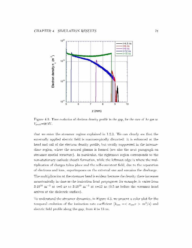
CHAPTER 4. SIMULATION RESULTS 78
Figure 4.1: Time evolution of electron density prole in the gap, for the case of Ar gas at
Vpeak=60 kV.
that we enter the streamer regime explained in 1.2.3. We can clearly see that the
externally applied electric eld is macroscopically distorted: it is enhanced at the
head and tail of the electron density prole, but totally suppressed in the interme-
diate region, where the neutral plasma is formed (see also the next paragraph on
streamer spatial structure). In particular, the rightmost region corresponds to the
non-stationary cathode sheath formation, while the leftmost edge is where the mul-
tiplication of charges takes place and the self-consistent eld, due to the separation
of electrons and ions, superimposes on the external one and sustains the discharge.
The multiplication at the streamer head is evident because the density there increases
monotonically in time as the ionization front propagates; for example, it varies from
3·1018 m−3 at t=6 ns to 3·1019 m−3 at t=12 ns (0.5 ns before the streamer head
arrives at the dielectric surface).
To understand the streamer dynamics, in Figure 4.3, we present a color plot for the
temporal evolution of the ionization rate coecient (kion =< σionv > m3/s) and
electric eld prole along the gap, from 4 to 13 ns.

CHAPTER 4. SIMULATION RESULTS 79
Figure 4.2: Time evolution of electric eld prole in the gap, for the case of Ar gas at
Vpeak=60 kV.
It is evident that, while the streamer propagates from the cathode to the anode, the
streamer head is where the ionization takes place with ionization frequencies greater
than 1010 s−1; the intermediate region is in fact characterised by such a weak eld
that no appreciable charge multiplication was expected there.
The ionization front reaches the dielectric surface at 12.48 ns, moving with an average
speed of 5.1·105 m/s, in agreement with the classical prediction based on a uid model
[43]. A large current density is measured at the dielectric, with a duration of slightly
less than 0.5 ns and with a maximum value of 2.25·106 A/m2. The maximum charge
density mesured at the dielectric is 2.3·10−4 C/m2. On the other hand, no current is
meaured at the cathode, i.e. ions can be considered 'frozen' in the timespan of the
applied signal (40 ns).
During the electric charge deposition on the dielectric surface, a non-zero ionization
rate is observed along the gap, with the exception of the rightmost region (about 1
mm from the cathode). This is due to the redistribution of the electric potential in
the gap: as the streamer head reaches the dielectric, the boundary conditions in the
gap change, and this causes the electric eld to penetrate in the bulk plasma, which

CHAPTER 4. SIMULATION RESULTS 80
had been eectively shielded up to now. A brief phase of charge multiplication is
thus sustained by this non-zero electric eld in a region with conspicuous electron
density. This also explains why, in Figure 4.1, the green density prole (t=15 ns) is
qualitatively dierent from the proles at 6, 9 and 12 ns.
Figure 4.3: Time evolution of ionization rate coecient and electric eld proles for the
case of Figure 4.1 and 4.2.

CHAPTER 4. SIMULATION RESULTS 81
Figure 4.4: Time evolution of electric eld prole corresponding to electric potential redis-
tribution in the gap following charge deposition at the dielectric surface.
The electric eld in the intermediate region is very rapidly suppressed, however, by
the enhanced plasma density in the gap; on the other hand, the high collisionality
causes the loss of electron energy. The entire phenomenon lasts less than 0.5 ns.
The extremely quick penetration and suppression of electric eld in the plasma bulk is
illustrated more clearly in Figure 4.4, where its evolution in the interval 12.48÷12.72ns is shown. We can clearly distinguish an initial phase of eld enhancement (rst
three curves) and a nal phase of eld suppression (last two curves).
The heating of electrons at the streamer head is evident in Figure 4.5, which is a
scatter plot of the macroelectrons population in phase space (z,vz), at four dierent
times. As the streamer front moves towards the anode, we distinguish an increasing
spread of the velocity distribution around1 vz=0, which is interpreted as an increase
in temperature (more precisely, mean energy). The black snapshot, corresponding1Naively, it might be thought that the distribution should be strongly asymmetric around vz=0,
because the electrons move leftward, but the eect of velocity spread is much more important.

CHAPTER 4. SIMULATION RESULTS 82
to t = 15 ns, is referred to the gap completely lled with plasma: the electric eld
is totally screened and the electron mean energy is too low to sustain ionization.
Figure 4.5: Scatter plot of macroelectrons population in phase space at t = 6, 9, 12 and
15 ns.
4.2 Streamer spatial structure
The spatial structure of the streamer can be illustrated with the aid of the following
two gures. The rst is a snapshot of the entire gap and shows both electron and
ion densities, along with electron temperature prole for Ar gas with Vpeak=30 kV
(reduced electric eld E/n=240 Td); the second shows a zoomed view of the streamer
head in the same case.
The prole shown can be subdivided in ve regions:
1. The leftmost region is where the temperature (violet curve, see Fig. 4.7) shows
a pronounced gradient in less than 5 Debye lengths, calculated using local
values of electron density and temperature. The latter has a maximum of 4

CHAPTER 4. SIMULATION RESULTS 83
Figure 4.6: Electron density, ion density and electron temperature proles along the entire
gap for the case of Ar gas and Vpeak=30 kV at t=17.4 ns
eV, which occurs around 0.05 mm ahead of the electron density peak. This
region is where the ionization rate and electric eld are high, and the electric
discharge is sustained.
We highlight the pronounced temperature uctuations in leftmost region of
the temperature prole, due to the very low electron density there. This can
be considered an unavoidable feature of the PIC method.
2. The streamer head is the region where a net negative space charge is observed,
see Fig. 4.7. This separation of positive and negative charges is responsible
for the plasma self-consistent eld, (see Fig. 4.2 and related comments). The
streamer head has a length of about 0.15 mm, corresponding to about 20 Debye
lengths; electron density reaches a maximum of 6·1018 m−3, then decreasing
until ion and electron densities become equal at about z = 5.45 mm, the
beginning of the plasma bulk.

CHAPTER 4. SIMULATION RESULTS 84
3. The plasma bulk is a neutral region where the electric eld is totally screened.
It constitutes the conductive channel which is left behind by the propagating
ionization front. We can see that both particle densities and electron temper-
ature decrease moving rightward. This last feature is a consequence of electric
eld suppression and high collisionality at atmospheric pressure.
4. The tail of the plasma bulk is characterized by a plasma density depression
and a rise in electron temperature; however, the latter is never greater than
0.06 eV, i.e. much smaller than the values measured in the streamer head, of
the order of few eV.
5. The cathode sheath, with a thickness of slightly less than 1.2 mm. The electron
density therein is practically zero while the ion density decreases from 1018 m−3
to zero moving towards the anode. This can be considered a matrix sheath; no
plasma is formed there despite the very large electric eld, because no electrons
can enter it.
Figure 4.7: Zoomed view of the streamer head region for the case of Fig. 4.6.
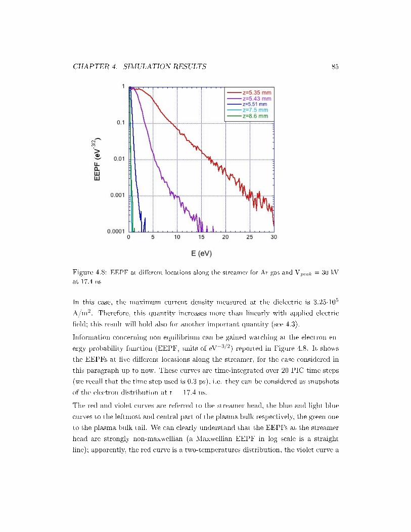
CHAPTER 4. SIMULATION RESULTS 85
Figure 4.8: EEPF at dierent locations along the streamer for Ar gas and Vpeak = 30 kV
at 17.4 ns
In this case, the maximum current density measured at the dielectric is 3.25·105
A/m2. Therefore, this quantity increases more than linearly with applied electric
eld; this result will hold also for another important quantity (see 4.3).
Information concerning non-equilibrium can be gained watching at the electron en-
ergy probability function (EEPF, units of eV−3/2) reported in Figure 4.8. It shows
the EEPFs at ve dierent locations along the streamer, for the case considered in
this paragraph up to now. These curves are time-integrated over 20 PIC time steps
(we recall that the time step used is 0.3 ps), i.e. they can be considered as snapshots
of the electron distribution at t = 17.4 ns.
The red and violet curves are referred to the streamer head, the blue and light blue
curves to the leftmost and central part of the plasma bulk respectively, the green one
to the plasma bulk tail. We can clearly understand that the EEPFs at the streamer
head are strongly non-maxwellian (a Maxwellian EEPF in log scale is a straight
line); apparently, the red curve is a two-temperatures distribution, the violet curve a
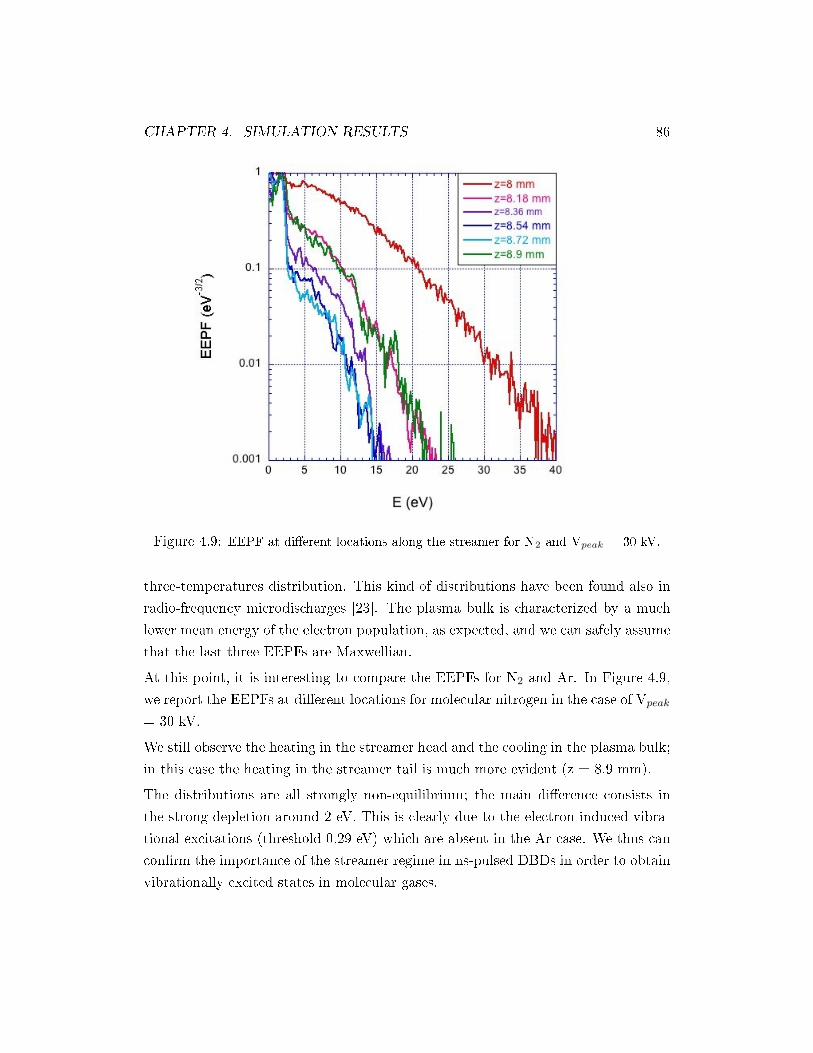
CHAPTER 4. SIMULATION RESULTS 86
Figure 4.9: EEPF at dierent locations along the streamer for N2 and Vpeak = 30 kV.
three-temperatures distribution. This kind of distributions have been found also in
radio-frequency microdischarges [23]. The plasma bulk is characterized by a much
lower mean energy of the electron population, as expected, and we can safely assume
that the last three EEPFs are Maxwellian.
At this point, it is interesting to compare the EEPFs for N2 and Ar. In Figure 4.9,
we report the EEPFs at dierent locations for molecular nitrogen in the case of Vpeak
= 30 kV.
We still observe the heating in the streamer head and the cooling in the plasma bulk;
in this case the heating in the streamer tail is much more evident (z = 8.9 mm).
The distributions are all strongly non-equilibrium; the main dierence consists in
the strong depletion around 2 eV. This is clearly due to the electron-induced vibra-
tional excitations (threshold 0.29 eV) which are absent in the Ar case. We thus can
conrm the importance of the streamer regime in ns-pulsed DBDs in order to obtain
vibrationally excited states in molecular gases.
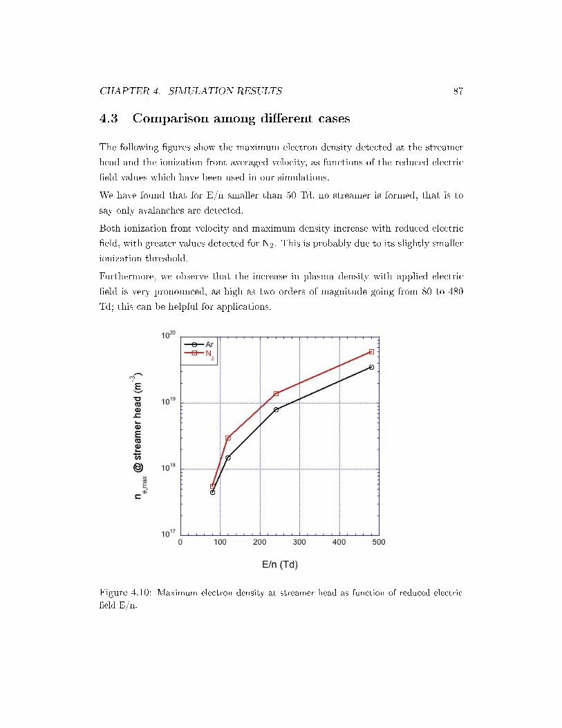
CHAPTER 4. SIMULATION RESULTS 87
4.3 Comparison among dierent cases
The following gures show the maximum electron density detected at the streamer
head and the ionization front averaged velocity, as functions of the reduced electric
eld values which have been used in our simulations.
We have found that for E/n smaller than 50 Td, no streamer is formed, that is to
say only avalanches are detected.
Both ionization front velocity and maximum density increase with reduced electric
eld, with greater values detected for N2. This is probably due to its slightly smaller
ionization threshold.
Furthermore, we observe that the increase in plasma density with applied electric
eld is very pronounced, as high as two orders of magnitude going from 80 to 480
Td; this can be helpful for applications.
Figure 4.10: Maximum electron density at streamer head as function of reduced electric
eld E/n.

CHAPTER 4. SIMULATION RESULTS 88
Figure 4.11: Ionization front averaged velocity as function of reduced electric eld E/n.

Conclusions
In this thesis work, we have considered dielectric barrier discharges at atmospheric
pressure, powered by a nanosecond pulsed trapezoidal signal applied to the exposed
electrode, for Ar and N2 gases. Traditionally, DBDs were powered in the kHz fre-
quency range, while the dynamics in the ns regime is relatively poor studied and
understood.
We have found clear evidence of the streamer regime as the breakdown mechanism
which sustains the discharge. The PIC/MCC method has allowed the spatial res-
olution of the streamer structure as it evolved and propagated along the gap; fur-
thermore, non-equilibrium has been conrmed as having an important role in the
streamer head, aecting the rate of inelastic processes occurring therein, while the
plasma formed in the intermediate region rapidly thermalize. Fluid models must
necessarily take into account the strong gradients at the streamer front which have
been highlighted in this and similar works, as well as the two- and three-temperatures
structure of the electron distribution functions.
Numerous extensions of our work (submitted and under review [44]) are possible and
must be implemented in order to give useful guidelines for applications and, from
a more fundamental point of view, to allow a more thorough understanding of the
streamer regime. As an example, it is necessary to extend our model from 1D to
3D, so that the radial structure of the streamer and the formation of geometrical
89
patterns on the dielectric surface could be analyzed; furthermore, photoionization
and photoemission must be included in order to study positive (i.e. cathode-directed)
streamers as well.
Also, it is necessary to consider a longer timespan (and possibly to include a multiple
rather than a single-shot signal) because, when the plasma is formed and occupies
the entire gap, the dynamics can change remarkably with respect to the case in which
the streamer breakdown is triggered starting from few macroelectrons.
Our values of plasma density, ionization front velocity and their dependence on
applied electric eld can however be used as benchmarks for uid simulations in the
same conditions, for example in the study of actuators.
Results based on fully kinetic (PIC) simulations will remain a fundamental tool for
electric discharge physics: on one hand, the spatial and temporal resolution allowed
are orders of magnitude greater than the ones permitted by even the most advanced
experimental probes, so that this is at present probably the best tool to investigate
the ne structure and time evolution of plasmas; on the other, PIC simulations can
consitute the test for theories trying to explain the most fundamental features of cold
plasmas at atmospheric pressure (e.g. a general theory of plasma sheath formation
is still missing at high pressure because of the high collisional frequency).
Cold plasmas have gained, in the last decades, a multitude of applications in a great
variety of elds. In principle, they oer the possibility of tailoring the electron distri-
bution function for a particular task, maximizing the rate coecient of a particular
reaction channel. A detailed knowledge of the physics involved in every regime can
thus open new paradigms, not only based on a trial-and-error kind of procedure, but
on a more sound basis.
90
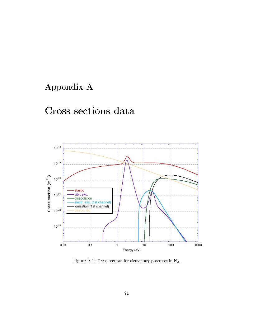
Appendix A
Cross sections data
Figure A.1: Cross sections for elementary processes in N2.
91
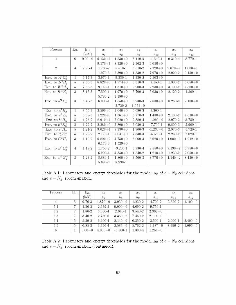
Table A.1: Parameters and energy thresholds for the modelling of e−N2 collisionsand e−N+
2 recombination.
Table A.2: Parameters and energy thresholds for the modelling of e−N2 collisionsand e−N+
2 recombination (continued).
92

Figure A.2: Cross sections for e-Ar elementary processes considered in our simulations; the
Ramsauer minimum is visible in the elastic cross section at 0.2 eV.
93

Appendix B
Box-Muller transform
The Box-Muller transform is a computationally ecient alternative to the inverse
transform method for generating random numbers (an example of which we have
seen in the Direct Monte Carlo scheme, par. 2.4). It allows to generate couples of
independent, normally distributed random numbers starting from couples of inde-
pendent, uniformly distributed random numbers in the interval [0, 1].
In fact, it can be shown that if R1 and R2 are two such numbers, then:
Z1 =√
−2 lnR1 cos(2πR2),
Z2 =√
−2 lnR1 sin(2πR2)
are gaussian, indipendent variables with zero expectation values and unit variance.
This is the basic form of the BM transform.
We use this approach every time we need to generate the velocity components of a
charged particle assumed distributed according to a Maxwellian. More explicitly, as
an example, when we inject the electrons and ions at the beginning of the simulation,
we use the BM transform twice:
vx =
√−2 lnR1
kBTe
mecos(2πR2)
vy =
√−2 lnR1
kBTe
mesin(2πR2)
94

the rst time, and a second time to generate vz for the present particle and the next
one.
The same is done for ions, with their temperature (300 K) and mass.
95

Bibliography
[1] Chen F., Introduction to Plasma Phyics, New York: Plenum Press, 1974
[2] Raizer Y. P., Gas Discharge Physics, Berlin Heidelberg: Springer, 2011
[3] Fridman A., Plasma Chemistry, New York: Cambridge University Press, 2008
[4] Lieberman M., Lichtenberg A., Principles of Plasma Discharges and Materials
Processing, Hoboken: John Wiley & Sons, 2005
[5] Roth J. R., Industrial Plasma Processing. 1. Principles, Bristol: Institute of
Physics Publishing, 1995
[6] Lozansky E. D., Firsov O. B., Theory of Sparks, Moscow: Atomizdat, 1975
[7] von Engel A., Handbuch der Physik Bd.21, Berlin: Springer, 1956
[8] Meek J.M., 'A theory of spark discharge', Phys. Rev. 57 (8), 722 (1940)
[9] Kunhardt E.E., Tzeng Y., 'Development of an electron avalanche and its tran-
sition into streamers', Phys. Rev. A 38 (3), 1410 (1988)
[10] Meek J. M., Craggs J. D., Electrical Breakdown of Gases, New York: Wiley,
1978
[11] Ebert, U., Brau, F., Derks, G., Hundsdorfer, W., Kao, C.Y., Li, C., Luque,
A., Meulenbroek, B., Nijdam, S., Ratushnaya, V., Schäfer, L., and Tanveer, S.,
'Multiple scales in streamer discharges, with an emphasis on moving boundary
approximations' Nonlinearity, 24, C1 (2011).
96

[12] Gherardi N., Gouda G., Gat E., Ricard A., Massines F., 'Transition from glow
silent discharge to micro-discharges in nitrogen gas', Plasma Sources Sci. Tech-
nol. 9 340 (2000)
[13] Massines F., Rabehi A., Decomps P., Ben Gadri R., Ségur P., 'Experimental
and theoretical study of a glow discharge at atmospheric pressure controlled by
dielectric barrier', J. Appl. Phys. 83 2950 (1998)
[14] Okazaki S, Kogoma M, Uehara M and Kimura Y, 'Appearance of stable glow
discharge in air, argon, oxygen and nitrogen at atmospheric pressure using a 50
Hz source' J. Phys. D: Appl. Phys. 26 889 (1993)
[15] Shin J., Raja L., Dynamics of pulse phenomena in helium dielectric-barrier
atmospheric-pressure glow discharges, J. Appl. Phys. 94 7408 (2003)
[16] ijacic D.D., Ebert U., Transition from townsend to glow discharge: subcritical,
mixed, or super- critical characteristics Phys. Rev. E 66 (6), 066410 (2002)
[17] Kanazawa S., Kogoma M., Moriwaki T. and Okazaki S., J. Phys. D: Appl. Phys.,
Stable glow plasma at atmospheric pressure 21 836 (1988)
[18] Shao T., Long K., Zhang C., Wang J., Zhang D., Yan P. and Zhang S., Electri-
cal characterization of dielectric barrier discharge driven by repetitive nanosec-
ond pulses in atmospheric air J. Electrostat. 67 215 (2009)
[19] Walsh J. L. and Kong M. G., 10 ns pulsed atmospheric air plasma for uniform
treatment of polymeric surfaces Appl. Phys. Lett. 91 251504 (2007)
[20] Sang C., Sun J., Wang D., Plasma density enhancement in atmospheric-
pressure dielectric-barrier discharges by high-voltage nanosecond pulse in the
pulse-on period: a PIC simulation , J. Phys. D: Appl. Phys. 43 045202 (2010)
[21] Starikovskii A. Y., Nikipelov A., Nudnova M. M., Roupassov D. V., Plasma
Sources Sci. Technol., SDBD plasma actuator with nanosecond pulse periodic
discharge 18 034015 (2009)
[22] Bruggeman P., Brandeburg R., Atmospheric pressure discharge laments and
microplasmas: physics, chemistry and diagnostics, J. Phys. D: Appl. Phys. 46
464001 (2013)
97
[23] Iza F., Lee J. K., Kong M. G., Electron Kinetics in Radio-Frequency
Atmospheric-Pressure Microplasmas, Phys. Rev. Lett. 99 075004 (2007)
[24] Taccogna F., Dilecce G., Non-equilibrium in low-temperature plasmas , Eur.
Phys. J. D 70 251 (2016)
[25] Kim H. C.,Iza F., Yang S. S., Radmilovi¢-Radjenovi¢ M., Lee J. K., Particle
and uid simulations of low-temperature plasma discharges: benchmarks and
kinetic eects, J. Phys. D: Appl. Phys. 38 R283R301 (2005)
[26] Unfer T., Boeuf J. P., Modelling of a nanosecond surface discharge actuator,
J. Phys. D: Appl. Phys. 42 194017 (2009)
[27] Buneman O., Dissipation of currents in ionized media Phys. Rev. 115 503-517
(1959)
[28] Dawson J. M., One-dimensional plasma model , Phys. Fluids, 5 445-459 (1962)
[29] Dawson J. M., Particle simulation of plasmas , Rev. Mod. Phys. 55 403 (1983)
[30] Hockney R. W., Eastwood J. W., Computer Simulation Using Particles, New
York: Hilger, 1988
[31] Courant R., Friedrichs K., Lewy H., On the Partial Dierence Equations of
Mathematical Physics, IBM J., 11 215-234 (1967)
[32] Taccogna F., Monte Carlo Collision method for low temperature plasma simu-
lation , J. Plasma Physics 81 (1) 305810102 (2015)
[33] Tskhakaya D., Matyash K., Schneider R., Taccogna F., The Particle-In-Cell
Method , Contrib. Plasma Phys. 47 (8-9) 563 (2007)
[34] Nanbu K., Probability Theory of ElectronMolecule, IonMolecule,
MoleculeMolecule, and Coulomb Collisions for Particle Modeling of Materi-
als Processing Plasmas and Gases, IEEE Trans. on Pl. Sci., 28 (3) (2000)
[35] Nanbu K., Kitatani Y., An ion-neutral species collision model for particle sim-
ulation of glow discharge, J. Phys. D: Appl. Phys. 28 324 (1995)
98

[36] Skullerud H. R., The stochastic computer simulation of ion motion in a gas
subjected to a constant electric eld, J. Phys. D: Appl. Phys. 1 1567-1569
(1968).
[37] Longo S., Monte Carlo models of electron and ion transport in non-equilibrium
plasmas , Plasma Sources Sci. Technol. 9 468 (2000)
[38] Tabata T., Shirai T., Sataka M., Kubo H., Analytic cross sections for elec-
tron impact collisions with nitrogen molecules, Atomic Data and Nuclear Data
Tables 92 375406 (2006)
[39] http://jila.colorado.edu/~avp/collision_data/electronneutral/
ELECTRON.TXT
[40] Green A., McNeal R. J., Analytic cross sections for inelastic collisions of protons
and hydrogen atoms with atomic and molecular gases, J. Geophys. Res. 76 133
(1971)
[41] Mul P. M., McGowan J. W., J. Phys. B 12 1591 (1979)
[42] Vincenti W. G., Kruger C. H. Jr, Introduction to Physical Gas Dynamics, New
York: Wiley, 1967
[43] Ebert U., van Saarloos W., Caroli C., Propagation and structure of planar
streamer fronts, Phys. Rev. E 55 1530 (1997)
[44] Taccogna F., Pellegrini F. (2017), Kinetics of Plasma Streamer, Submitted to:
Journal of Physics D: Applied Physics
99
Recommended