Paraphrases for Statistical Machine Translationby
Ramtin Mehdizadeh Seraj
B.Sc., Amirkabir University of Technology, 2013
Thesis Submitted in Partial Fulfillment
of the Requirements for the Degree of
Master of Science
in the
School of Computing Science
Faculty of Applied Sciences
c© Ramtin Mehdizadeh Seraj 2015SIMON FRASER UNIVERSITY
Fall 2015
All rights reserved.However, in accordance with the Copyright Act of Canada, this work may be reproduced
without authorization under the conditions for “Fair Dealing.” Therefore, limitedreproduction of this work for the purposes of private study, research, criticism, review andnews reporting is likely to be in accordance with the law, particularly if cited appropriately.
Approval
Name: Ramtin Mehdizadeh Seraj
Degree: Master of Science (Computing Science)
Title: Paraphrases for Statistical Machine Translation
Examining Committee: Dr. Arrvindh Shriraman (chair)Assistant Professor
Dr. Anoop SarkarSenior SupervisorProfessor
Dr. Fred PopowichSupervisorProfessor
Dr. Giuseppe CareniniExternal ExaminerAssociate ProfessorDepartment of Computer ScienceUniversity of British Columbia
Date Defended: Sep 25th, 2015
ii
Abstract
Statistical Machine Translation (SMT) is the task of automatic translation between two natural
languages (source language and target language) by using bilingual corpora. To accomplish this
goal, machine learning models try to capture human translation patterns inside a bilingual cor-
pus. An open challenge for SMT is finding translations for phrases which are missing in the
training data (out-of-vocabulary phrases). We propose to use paraphrases to provide translations
for out-of-vocabulary (OOV) phrases. We compare two major approaches to automatically ex-
tract paraphrases from corpora: distributional profile (DP) and bilingual pivoting. The multilingual
Paraphrase Database (PPDB) is a freely available automatically created (using bilingual pivoting)
resource of paraphrases in multiple languages. We show that a graph propagation approach that
uses PPDB paraphrases can be used to improve overall translation quality. We provide an extensive
comparison with previous work and show that our PPDB-based method improves the BLEU score
by up to 1.79 percent points. We show that our approach improves on the state of the art in three
different settings: when faced with limited amount of parallel training data; a domain shift between
training and test data; and handling a morphologically complex source language.
Keywords: Natural Language Processing; Statistical Machine Translation; Paraphrase Database;
resource poor languages; morphologically complex languages; Graph-based semi-supervised method;
multilingual resources; PPDB; out-of-vocabulary; OOV
iii

Dedication
To my loving parents whose words of encouragement and push for tenacity ring in my ears.
iv
Acknowledgements
First, I would like to express my endless gratitude towards my senior supervisor Dr. Anoop Sarkar,
for his brilliant insights, encouragement, and patience during my Master’s career. Without his great
supervision this work would not have been possible. I have been very fortunate to have Dr. Fred
Popowich and Dr. Giuseppe Carenini on my committee and their valuable comments and feedback
helped me improve this thesis, of which I am appreciative. Several people in the Department of
Computing Science helped along the way. I am grateful to Dr. Greg Mori, Dr. Oliver Schulte,
Dr. Alexandra Fedorova.
I learned a lot from the present and past members who have been my colleagues in the Natural
Language Processing lab (natlang). Many ideas were developed in discussions with Mark Schmidt,
Maryam Siahbani, Jasneet Sabharwal, Baskaran Sankaran, Anahita Mansouri, Golnar Sheikhshab,
Mehdi Soleimani, Hassan Shavarani, Bradley Ellert, Ann Clifton, Rohit Dholakia, Milan Tofiloski,
Bruce Krayenhoff. I owe special thanks to Maryam Siahbani for all of the brainstorming during the
course of writing this dissertation. Outside of the lab, I thank Arash Vahdat, Mehran Khodabande,
Hossein Hajimirsadeghi, Sajjad Gholami, Hengameh Mirzaalian, Nastaran Hajinazar.
I had a whale of time in Vancouver. This I owe to the friends I spent time with: Bamdad, Sanam,
Mahsa, Sina, Atiyeh, Amirabbas, Ali, Haniye, Mehran, Mahan, Behdad, and Sara. Thank you all
for keeping me sane.
Finally, I would like to express my gratitude towards my family. I am extremely fortunate for
having been blessed with my incredible parents who always supported me with their unconditional
love.
v
Table of Contents
Approval ii
Abstract iii
Dedication iv
Acknowledgements v
Table of Contents vi
List of Tables viii
List of Figures ix
1 Introduction 11.1 Motivation . . . . . . . . . . . . . . . . . . . . . . . . . . . . . . . . . . . . . . . 1
1.2 Comparison to Related Work . . . . . . . . . . . . . . . . . . . . . . . . . . . . . 3
1.3 Contributions . . . . . . . . . . . . . . . . . . . . . . . . . . . . . . . . . . . . . 5
1.4 An Overview of This Thesis . . . . . . . . . . . . . . . . . . . . . . . . . . . . . 5
2 Background 72.1 Generative Machine Translation . . . . . . . . . . . . . . . . . . . . . . . . . . . 7
2.1.1 Language Modelling . . . . . . . . . . . . . . . . . . . . . . . . . . . . . 8
2.1.2 Translation Modeling . . . . . . . . . . . . . . . . . . . . . . . . . . . . . 9
2.2 Discriminative Machine Translation . . . . . . . . . . . . . . . . . . . . . . . . . 13
2.3 Evaluation of MT Systems . . . . . . . . . . . . . . . . . . . . . . . . . . . . . . 14
2.4 Semi-Supervised Learning (SSL) . . . . . . . . . . . . . . . . . . . . . . . . . . . 15
2.4.1 Transductive versus Inductive . . . . . . . . . . . . . . . . . . . . . . . . 15
2.4.2 Graph Based methods . . . . . . . . . . . . . . . . . . . . . . . . . . . . 16
2.5 Summary . . . . . . . . . . . . . . . . . . . . . . . . . . . . . . . . . . . . . . . 16
3 Automatic Paraphrase Extraction Methods 173.1 Paraphrases from Distributional Profiles . . . . . . . . . . . . . . . . . . . . . . . 17
3.2 Paraphrases from Bilingual Pivoting . . . . . . . . . . . . . . . . . . . . . . . . . 19
vi
3.2.1 PPDB . . . . . . . . . . . . . . . . . . . . . . . . . . . . . . . . . . . . . 20
3.3 Summary . . . . . . . . . . . . . . . . . . . . . . . . . . . . . . . . . . . . . . . 22
4 Methodology 234.1 Overview . . . . . . . . . . . . . . . . . . . . . . . . . . . . . . . . . . . . . . . 23
4.2 Transferring Translations . . . . . . . . . . . . . . . . . . . . . . . . . . . . . . . 24
4.2.1 Naive Approach . . . . . . . . . . . . . . . . . . . . . . . . . . . . . . . 24
4.2.2 Graph Propagation . . . . . . . . . . . . . . . . . . . . . . . . . . . . . . 24
4.3 Phrase Table Integration . . . . . . . . . . . . . . . . . . . . . . . . . . . . . . . 29
4.4 Summary . . . . . . . . . . . . . . . . . . . . . . . . . . . . . . . . . . . . . . . 29
5 Analysis of the Framework 305.1 Propagation of poor translations . . . . . . . . . . . . . . . . . . . . . . . . . . . 30
5.1.1 Graph pruning and PPDB sizes . . . . . . . . . . . . . . . . . . . . . . . . 30
5.1.2 Pruning the translation candidates . . . . . . . . . . . . . . . . . . . . . . 31
5.1.3 External Resources for Filtering . . . . . . . . . . . . . . . . . . . . . . . 32
5.2 Path sensitivity . . . . . . . . . . . . . . . . . . . . . . . . . . . . . . . . . . . . 32
5.2.1 Pre-structuring the graph . . . . . . . . . . . . . . . . . . . . . . . . . . . 33
5.2.2 Graph random walks . . . . . . . . . . . . . . . . . . . . . . . . . . . . . 33
5.2.3 Early stopping of propagation . . . . . . . . . . . . . . . . . . . . . . . . 33
5.3 Summary . . . . . . . . . . . . . . . . . . . . . . . . . . . . . . . . . . . . . . . 33
6 Evaluation 346.1 Experimental Setup . . . . . . . . . . . . . . . . . . . . . . . . . . . . . . . . . . 34
6.2 Impact of OOVs: Oracle experiment . . . . . . . . . . . . . . . . . . . . . . . . . 35
6.3 Case 1: Limited Parallel Data . . . . . . . . . . . . . . . . . . . . . . . . . . . . . 37
6.4 Case 2: Domain Adaptation . . . . . . . . . . . . . . . . . . . . . . . . . . . . . . 38
6.5 Case 3: Morphologically Rich Languages . . . . . . . . . . . . . . . . . . . . . . 38
6.6 Examples . . . . . . . . . . . . . . . . . . . . . . . . . . . . . . . . . . . . . . . 39
6.7 Summary . . . . . . . . . . . . . . . . . . . . . . . . . . . . . . . . . . . . . . . 39
7 Conclusion and Future work 407.1 Future work . . . . . . . . . . . . . . . . . . . . . . . . . . . . . . . . . . . . . . 40
Bibliography 42
vii
List of Tables
Table 3.1 A subset of PPDB showing paraphrases in different levels . . . . . . . . . . 20
Table 3.2 Scoring paraphrase pairs by linear combination of features inside the PPDB . 21
Table 3.3 English PPDB version 1 statistics (number of rules) . . . . . . . . . . . . . 21
Table 4.1 Naive approach example . . . . . . . . . . . . . . . . . . . . . . . . . . . . 24
Table 4.2 Statistics of the graph constructed using the English lexical PPDB . . . . . . 25
Table 4.3 Phrase table augmentation with the new phrase pairs . . . . . . . . . . . . . 29
Table 6.1 Statistics of OOVs for each setting in Sec. 6. . . . . . . . . . . . . . . . . . 35
Table 6.2 The impact of translating OOVs. . . . . . . . . . . . . . . . . . . . . . . . 35
Table 6.3 Case 1: Limited Parallel Data - Results of PPDB and DP techniques . . . . . 37
Table 6.4 Case 2: Domain Adaptation - Results of PPDB and DP techniques . . . . . 38
Table 6.5 Case 3: Morphologically Rich Source Language - Results of PPDB and DP
techniques for Arabic-English. . . . . . . . . . . . . . . . . . . . . . . . . . 39
Table 6.6 Examples comparing DP versus PPDB outputs on the test sets. . . . . . . . 39
viii
List of Figures
Figure 2.1 An example of alignments between an English sentences and a German
Sentence. . . . . . . . . . . . . . . . . . . . . . . . . . . . . . . . . . . 9
Figure 2.2 Architecture of a generative machine translation system. . . . . . . . . . . 12
Figure 2.3 Architecture of a descriminative machine translation system. . . . . . . . 13
Figure 2.4 Cases that unlabeled data can improve decision boundary selection. . . . . 15
Figure 3.1 A good example of distributional profiling for extracting paraphrase. . . . 18
Figure 3.2 A bad example of distributional profiling for extracting paraphrase. . . . . 19
Figure 3.3 English paraphrases extracted by pivoting over German shared translation. 20
Figure 4.1 An overview of an SMT system . . . . . . . . . . . . . . . . . . . . . . . 23
Figure 4.2 Modified Adsorption objective function visualization. . . . . . . . . . . . 26
Figure 4.3 Graph propagation feature 1 - filtering unrelated translations . . . . . . . 27
Figure 4.4 Graph propagation feature 2 - multi-hop translation transferring . . . . . . 27
Figure 4.5 Graph propagation feature 3 - enriching translation options for morpholog-
ical variants of a phrase . . . . . . . . . . . . . . . . . . . . . . . . . . . 28
Figure 4.6 A small sample of the real graph constructed from the Arabic PPDB for
Arabic to English translation . . . . . . . . . . . . . . . . . . . . . . . . 28
Figure 5.1 Cases that K-nearest neighbours graph pruning fails. . . . . . . . . . . . . 31
Figure 5.2 Cases that e-neighbourhood graph pruning fails. . . . . . . . . . . . . . . 31
Figure 5.3 Effect of PPDB size on improving BLEU score. . . . . . . . . . . . . . . 32
Figure 5.4 Sensitivity issue in graph propagation for translations. “Lager” is a trans-
lation candidate for “stock”, which is transferred to “majority” after 3 iter-
ations. . . . . . . . . . . . . . . . . . . . . . . . . . . . . . . . . . . . . 32
Figure 6.1 The structure of oracle experiment for baseline . . . . . . . . . . . . . . . 35
Figure 6.2 The structure of oracle experiment for lexical OOVs . . . . . . . . . . . . 36
Figure 6.3 The structure of oracle experiment for phrasal OOVs . . . . . . . . . . . 36
Figure 6.4 The structure of oracle experiment for complete OOVs . . . . . . . . . . 36
Figure 7.1 SMT results for infrequent phrases. . . . . . . . . . . . . . . . . . . . . 41
ix
Chapter 1
Introduction
1.1 Motivation
Statistical Machine Translation (SMT) is the task of translating between two languages by exploit-
ing bilingual parallel corpora using data-driven machine learning techniques. A parallel corpus
is a sequence of sentences in the source language with human provided translations in the target
language. Such parallel corpora are often available from sources such as parliament proceedings or
similar venues where multi-lingual data is created in large scale by trained human translators. These
techniques automatically capture co-occurrence relations between words in the source language and
corresponding words in the target language.These word alignments are used to extract phrase trans-
lation rules along with several probabilistic feature functions. These stochastic translation rules are
combined using a discriminative log-linear model. The weights for this log-linear model are learned
by minimizing a loss function that rewards matches against human translations.
After recent achievements in SMT, many potential applications, e.g. real time multilingual
translation in e-commerce websites, have been emerging very fast. Despite satisfactory results in
some of these applications, many of them are facing problems caused by a rudimentary assumption
in most SMT methods: availability of sufficient parallel corpora; this assumption, high dependence
of methods on existence of parallel corpora, is not true in many cases and limits the progress.
First case comes up when a limited amount of parallel data exists for resource poor languages.
With over 6,500 world natural languages, such large bilingual corpora are only available for the
official languages of the European Union (EU), Arabic, Chinese, and Russian. This problem become
worse considering language pairs instead of individual languages [50]. Lack of resources in these
languages, in the first step will increase Out-of-vocabulary (OOV) words, unseen words in bilingual
corpus, which dramatically reduce translation quality and fluency. The quality is not desirable due
to lack of translation for these new words, and also this has an adverse effect on reordering models
inside decoder resulting in reduced fluency.
Even for resource rich languages, lack of resources in certain domains (e.g. biomedical) leads
to poor quality translations (second case). Domain shift increases the number of OOVs and also
1
might cause nonsensical translations for phrases. For example, in social networks like Twitter,
several spelling variants of existing words and informal words are missing in the training set, which
requires domain adaptations methods. Even with a training data size of 10 million word tokens,
source vocabulary coverage in unseen data does not go above 90% [10]. The problem is worse with
multi-word OOV phrases.
Morphologically complex languages (e.g. Finnish, Arabic, ...) present the third case of situ-
ations, in which MT systems will not come up with words forms that have not observed. Many
of morphological variants of a phrase are missing even in high amount of parallel corpora, which
reduce the chance of finding a correct translation. For example, Arabic verbs, as in other Semitic
languages, are extremely complex; many grammatical functions like tense, person, number, mood,
voice are applied on a root made up of three consonants to build a correct verb for a sentence.
This fact exacerbates the sparsity problem for these languages; in other words, the more complex
structure a language has, the more data a machine translation system requires to capture the right
translation patterns.
Copying OOVs to the output is the most common solution. However, even noisy translations of
OOVs can improve reordering and language model scores [73]. Obtaining more parallel data is time
consuming, expensive, and requires domain experts. Although alternatives to alleviate this problem
like crowdsourcing in [58] have been suggested, achieving more parallel data is not always feasible
for machine translation. Transliteration is not a panacea for the OOV problem [28]. OOVs can be
divided into two categories: 1) named entities 2) non-named entities. Identifying named entities
like person names, organizations, dates, etc. inside a text, is another task in NLP. For the first
category, applying deterministic approaches like transliteration on top of identified named-entites in
the source side, provides good translations. Our target in this thesis is non-named entities, therefore
we find and remove the named entities, dates, etc. in the source and focus on the use of paraphrases
to help translate the remaining OOVs. In Chapter 6 we show that handling such OOVs correctly
does improve translation scores.
All of these cases illuminate the need of incorporating other types of resources including mono-
lingual corpus on the source side, paraphrase databases, dictionaries, morphological analyzers and
bridge language resources. Therefore, new robust methods that do not just rely on parallel corpora
are required to tackle these problems. For instance, [36] was one of the earliest works to find lexical
translations by using monolingual resources of the source and target language.
In this thesis, we build on the following research: Bilingual lexicon induction is the task of
learning translations of words from monolingual data from the source and target [64, 37, 24]. The
distributional profile (DP) approach uses context vectors to link words as potential paraphrases to
translation candidates [59, 37, 24, 22]. DPs have been used in SMT to assign translation candidates
to OOVs [45, 16, 29, 27]. Graph-based semi-supervised methods extend this approach and prop-
agate translation candidates across a graph with phrasal nodes connected via weighted paraphrase
relationships [60, 62]. Saluja et al. extend paraphrases for SMT from the words to phrases, which
we also do in this work [62]. Bilingual pivoting uses parallel data instead of context vectors for
2
paraphrase extraction [43, 64, 3, 10, 76, 9]. Ganitkevitch and his colleagues [20] published a large-
scale multilingual Paraphrase Database (PPDB) 1 which includes lexical, phrasal, and syntactic
paraphrases (with 170 million paraphrases for 22 languages).
PPDB is a natural resource for paraphrases. However, PPDB was not built with the specific
application to SMT in mind. Other applications such as text-to-text generation have used PPDB [21]
but SMT brings along a specific set of concerns when using paraphrases: translation candidates
should be transferred suitably across paraphrases. There are many cases, e.g. when faced with
different word senses where transfer of a translation is not appropriate. Our proposed methods of
using PPDB use graph propagation to transfer translation candidates in a way that is sensitive to the
mentioned SMT concerns.
Using PPDB has several advantages: 1) Resources such as PPDB can be built and used for
many different tasks including but not limited to SMT. 2) PPDB contains many features that are
useful to rank the strength of a paraphrase connection and with more information than distributional
profiles. 3) Paraphrases in PPDB are often better than paraphrases extracted from monolingual or
comparable corpora because a large-scale multilingual paraphrase database such as PPDB can pivot
through a large amount of data in many different languages. It is not limited to using the source
language data for finding paraphrases which distinguishes it from previous uses of paraphrases for
SMT.
Our framework has three stages: 1) a novel graph construction approach for PPDB paraphrases
linked with phrases from parallel training data. 2) Graph propagation that uses PPDB paraphrases.
3) An SMT model that incorporates new translation candidates. Chapter 4 explains these three
stages in detail.
1.2 Comparison to Related Work
There have been some attempts in using paraphrases to improve the performance of machine trans-
lation in different levels. Paraphrase pairs can be defined as lexical paraphrases, phrasal paraphrases
and sentential paraphrases.
Sentence level paraphrasing has been used to generate alternative reference translations to im-
prove discriminative training for SMT [42, 31], or augmenting the training data with sentential
paraphrases [5, 49, 47]. Using sentence level paraphrases to augment the underlying SMT model is
not scalable as there are exponentially many paraphrases if you consider each phrase in a sentence.
Another line of work, is to use lexical/phrasal paraphrases, hence human-generated version of
these resources are not available. Resnik et al (2010) use crowd-sourcing to obtain paraphrases for
source phrases corresponding to mistranslated target phrase [61]. Although using crowd-sourcing,
this approach is expensive and also is not applicable to all languages and domains. Thus, it is
essential to have accurate automatic ways to find paraphrase pairs. Many possible solution for auto-
matic paraphrase extraction has been proposed, one of the recent ones, is to use word embeddings1http://paraphrase.org
3
extracted using neural networks (i.e. the continuous representations often tend to cluster similar
words). Although these bilingual and multilingual word and phrase representation using neural net-
works have been applied to machine translation successfully [77, 46, 72], these embeddings are not
accurate for rare word or phrases [75]. Since having accurate (high precision) paraphrases espe-
cially for OOVs is a must for our problem, we decided not to use these methods. The remaining
two major ways of extracting paraphrases are: distributional profiling and bilingual pivoting which
is discussed in Chapter 3 in details. The first one uses monolingual corpora to extract paraphrases
while the second one uses bilingual resources.
Back to our problem, we want to use lexical/phrasal paraphrase pairs to improve translation
quality and alleviate the problem of OOV phrases. To improve the OOV phrase coverage different
parts of SMT can be altered. Two of the promising ones are changing the decoding stage and
augmenting phrase table. There are some works on using phrasal paraphrasing in lattice decoding
as well [55, 17]. They build paraphrase lattices for the source sentences which is given to the
lattice decoder to select the best one. Alexandrescu and Kirchhoff (2009) [1] use a graph-based
semi-supervised model determine similarities between sentences, then use it to re-rank the n-best
translation hypothesis. Liu et al. (2012) [41] extend this model to derive some features to be used
during decoding. These approaches are dependent on the decoding technique and are orthogonal
to our approach. Our approach, which is in the second category, augment the phrase table and any
type of decoder can benefits from that.
Similar to our approach, in augmenting the phrase table, Irvine and her colleagues [27] generate
a large, noisy phrase table by composing unigram translations which are obtained by a supervised
method from a limited parallel data and a bilingual lexicon induced from monolingual data [26].
Comparable monolingual data is used to re-score and filter the phrase table. Zhang et al. [74] use a
large manually generated lexicon for domain adaptation.
As mentioned before, the most similar works to ours are done by Razmara et al. and Saluja
et al. [60, 62]. [60] use graph-based semi-supervised methods extend this approach and propagate
translation candidates across a graph with phrasal nodes connected via weighted paraphrase rela-
tionships. Saluja et al. (2014) [62] extend the previous work by using Structured Label Propaga-
tion [41] in two parallel graphs constructed on source and target paraphrases. Our work is different
from their work in many aspects. First, we used a different (less noisy) approach to extract para-
phrases (bilingual pivoting) than distributional profiling. Second, their work is not scalable to the
n-grams longer than trigrams and extremely expensive, but our PPDB-based approach covers any
length phrases. Finally, because of different accurate filters used for extracting PPDB paraphrases,
in experiments we showed that it has a better performance when compared to the work by Razmara
et al. [60]. We can not directly compare our results to [62] because they exploit several external
resources such as a morphological analyzer and also had different sizes of training and test. In our
experiments (Chapter 6) we obtained comparable BLEU score improvement on Arabic-English by
using bilingual pivoting only on source phrases. [62] also use methods similar to [23] that expand
the phrase table with spelling and morphological variants of OOVs in test data.
4
1.3 Contributions
The primary contributions of this thesis can be summarized as follows:
• For the first time, we did a comprehensive study of the use of PPDB for statistical machine
translation model training. We showed that this resource is useful in all mentioned cases that
SMT suffers from a lack of translation for OOVs.
• We compare two major approaches of paraphrase extraction methods (PPDB versus DP) in
terms of their effectiveness in solving OOVs problem.
• We introduce a novel method for constructing a graph out of PPDB, and analyze the advan-
tageous and drawbacks of different graph construction methods. We also evaluate the impact
of constraints like graph pruning (K-nearest neighbours or e-radius) on improving our frame-
work.
1.4 An Overview of This Thesis
The chapters in this thesis are organized as follows:
Chapter 2 provides relevant background from the machine learning and machine translation liter-
ature. This chapter will covers definition and explanation of Statistical Machine Translation
approaches from different perspectives. A brief survey of semi-supervised machine learning
techniques is the last section of this chapter.
Chapter 3 introduce and compare major ways to automatically extract paraphrase pairs for a lan-
guage (DP versus PPDB). Distributional profiling (DP) uses monolingual corpora to find
paraphrases according to context, while (PPDB) uses bilingual pivoting over a parallel cor-
pus, to find paraphrases.
Chapter 4 explores possible approaches to transfer translations from seen phrases to unseen phrases.
We compare possible options and explain our framework step by step and its desirable fea-
tures.
Chapter 5 analyze our framework in terms of sensitivity to error and required consideration for
SMT. we discuss potential ways to improve the performance of our approach.
Chapter 6 compares our approach with the state-of-the-art in three different settings in SMT: 1)
when faced with limited amount of parallel training data; 2) a domain shift between training
and test data; and 3) handling a morphologically complex source language. In each case, we
show that our PPDB-based approach outperforms the distributional profile approach.
5

Chapter 7 summarizes the specific results achieved in the previous chapters on improving statis-
tical machine translations by using paraphrases. I then discuss possible avenues for future
research.
6
Chapter 2
Background
This chapter covers the background material for the topics that are relevant for this thesis. We
start by defining and explaining Statistical Machine Translation approaches (Generative versus Dis-
criminative). We illustrate levels of generative models (word-base, phrase-based and hierarchical),
followed by a brief description of word-alignment, language model and automatic machine transla-
tion evaluation measures. Then, we introduce discriminative machine translation methods. Finally,
we review semi-supervised machine learning approaches and close this chapter with a discussion
on a graph-based semi-supervised methods and their importance.
2.1 Generative Machine Translation
Machine Translation (MT) is the attempt to automate the process of translating from one natural
language (F ) to another (E). Statistical machine translation (SMT) is an approach to MT charac-
terized by the use of machine learning techniques. SMT models break languages into small units,
sentences, and try to translate sentence independently, based on the assumption that each sentence
conveys sufficient information. Therefore, the input of the most of machine translation models is a
large collection of sentences in the source language and it’s corresponding human translation in the
target language (parallel corpus or bitext).
Bitext(F,E) = {(f1, e1), (f2, e2), (f3, e3), . . . | fi/ei is in source (F) / target language (E) }
Given a source sentence f (e.g. French sentence), our MT model tries to find the target sentence
e (e.g. English sentence), that is most likely translation; in other words, given f , it search for the e
that maximize the probability P (e|f). Because of the close relationship of machine translation to
decipherment this step is called decoding.
best translation = argmaxe∈EP (e|f) (2.1)
7

Searching over all sentence in language E is very time consuming and not feasible even if you
limit the length of English translations to arbitrary length. To tackle this problem, by exploiting
Bayes Rule and The Noisy Channel concept, the above formula can be rewritten as :
argmaxe∈EP (e|f) = argmaxe∈EP (e) · P (f |e)P (f) (2.2)
Note that p(f) is a fix number inside the argmax and can be ignored.
argmaxe∈EP (e|f) = argmaxe∈EP (e) · P (f |e) (2.3)
This generative model has many benefits such as separating the score of fluency P (e) and trans-
lation score P (f |e). The first term, P (e), is the probability of sentence e in the language E and
the second one, P (f |e), is the probability translating sentence e into sentence f . But, where P (e)and P (f |e) are coming from? The two following subsections explains how to compute these prob-
abilities, where the first one is called language model and the second one is translation model. In
decoding stage, steps of generation of the target translation e from the source sentence f is the fol-
lowing: Segment the sentence f into units of translations, find the translations of these units in a
bilingual dictionary, and finally reorder the translated phrases.
2.1.1 Language Modelling
The goal of language modelling is to compute probability of occurrence of each sentence e in the
language E; which a good measure to see how fluent a sequence of words e = w0 w1 w2 w3 . . . is
in this language [7]. To find such a probability distribution, in the simplest case we can compute the
frequency of occurrence of each word and then multiply them to find probability of sentence e.
P (e) = p(w0) · p(w1) · p(w2) . . . (2.4)
This approach seems pretty straight forward, but it ignores the context around each word. To fix this
issue, computers break sentences into smaller substrings bigger than word. An n-word substring is
called an n-gram. Computing counts for each n-gram will help to capture more information about
the context of each word. For example, after computing counts for bi-grams we can compute the
probability of sentence e by multiplying conditional probabilities of words.
P (e) = p(w0) · p(w1|w0) · p(w2|w1) . . . (2.5)
Now this question comes into mind that why not moving to bigger n-grams or why not just using
occurrence of sentences by themselves in the language. The answer is sparsity. When moving to
higher n-grams, more training data are required. Even in computing counts for tri-grams, many of
the possible trigrams are missing inside the training data. Smoothing techniques can alleviate this
8
problem by saving probabilities for cases not observed before, but it can not completely solve this
problem.
2.1.2 Translation Modeling
Computing P (f |e) is more tricky than computing P (e), since monolingual resources are more
available than bilingual resources. P (f |e) is the target in this thesis, and we would like to provide
probability distribution for unseen e inside the training data.
Word-based Translation Models
Translation models can be computed in several levels based on their unit of translation.The first
level is to do the translation considering words as units of translations [6, 8, 4]. To do so, the
model should compute the probability distribution over possible translations for given a word in the
source language. Word-based machine translation models exploits unsupervised machine learning
techniques (e.g Expectation Maximization(EM), Variational Bayes, . . . ) to compute mentioned
probability distribution. Fundamentally, alignment is the task of producing bisegmentation relations
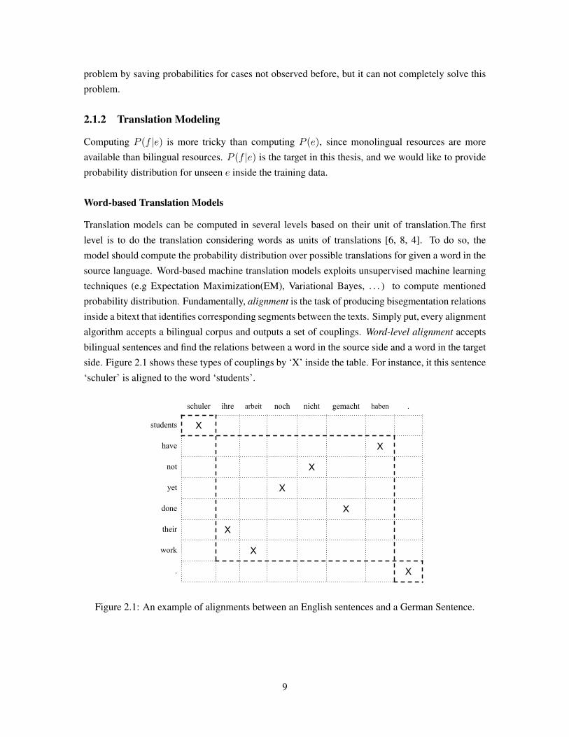
inside a bitext that identifies corresponding segments between the texts. Simply put, every alignment
algorithm accepts a bilingual corpus and outputs a set of couplings. Word-level alignment accepts
bilingual sentences and find the relations between a word in the source side and a word in the target
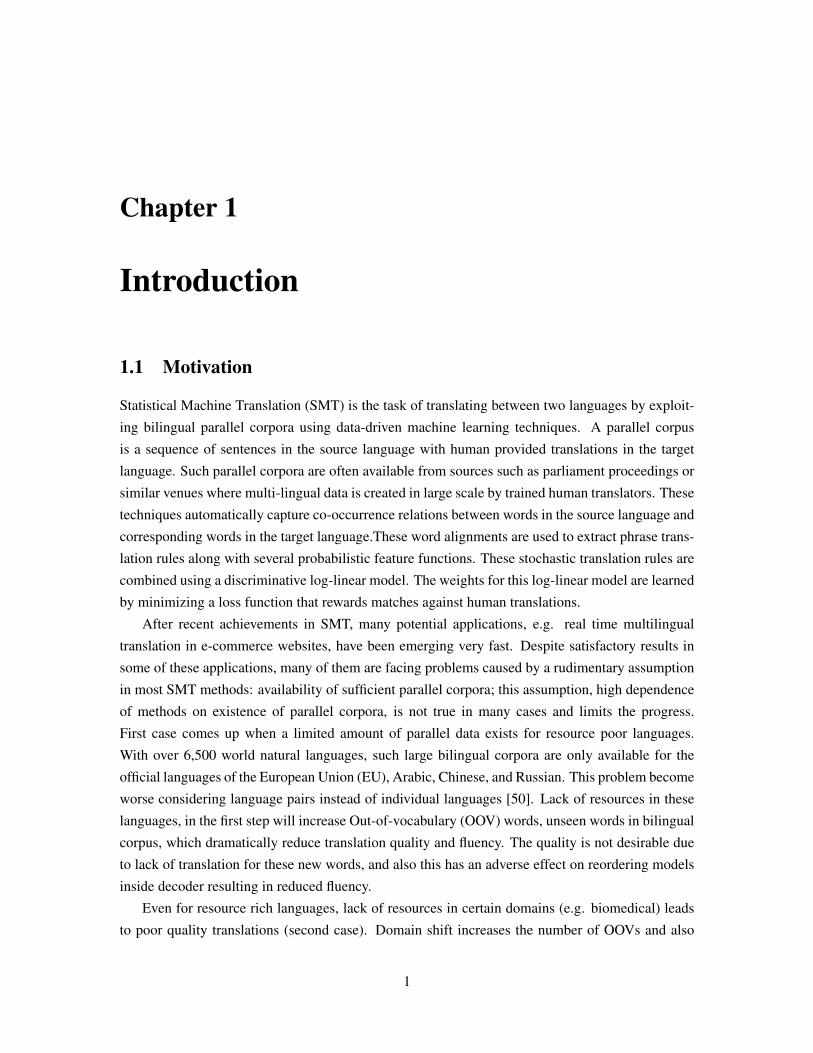
side. Figure 2.1 shows these types of couplings by ‘X’ inside the table. For instance, it this sentence
‘schuler’ is aligned to the word ‘students’.
schuler ihre arbeit noch nicht gemacht haben .
students X
have X
not X
yet X
done X
their X
work X
. X
Figure 2.1: An example of alignments between an English sentences and a German Sentence.
9
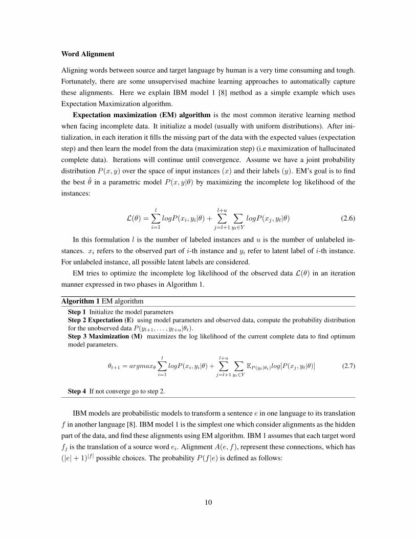
Word Alignment
Aligning words between source and target language by human is a very time consuming and tough.
Fortunately, there are some unsupervised machine learning approaches to automatically capture
these alignments. Here we explain IBM model 1 [8] method as a simple example which uses
Expectation Maximization algorithm.
Expectation maximization (EM) algorithm is the most common iterative learning method
when facing incomplete data. It initialize a model (usually with uniform distributions). After ini-
tialization, in each iteration it fills the missing part of the data with the expected values (expectation
step) and then learn the model from the data (maximization step) (i.e maximization of hallucinated
complete data). Iterations will continue until convergence. Assume we have a joint probability
distribution P (x, y) over the space of input instances (x) and their labels (y). EM’s goal is to find
the best θ in a parametric model P (x, y|θ) by maximizing the incomplete log likelihood of the
instances:
L(θ) =l∑
i=1logP (xi, yi|θ) +
l+u∑j=l+1
∑yt∈Y
logP (xj , yt|θ) (2.6)
In this formulation l is the number of labeled instances and u is the number of unlabeled in-
stances. xi refers to the observed part of i-th instance and yi refer to latent label of i-th instance.
For unlabeled instance, all possible latent labels are considered.
EM tries to optimize the incomplete log likelihood of the observed data L(θ) in an iteration
manner expressed in two phases in Algorithm 1.
Algorithm 1 EM algorithmStep 1 Initialize the model parametersStep 2 Expectation (E) using model parameters and observed data, compute the probability distributionfor the unobserved data P (yl+1, . . . , yl+u|θt).Step 3 Maximization (M) maximizes the log likelihood of the current complete data to find optimummodel parameters.
θt+1 = argmaxθ
l∑i=1
logP (xi, yi|θ) +l+u∑j=l+1
∑yt∈Y
EP (yt|θt)log[P (xj , yt|θ)] (2.7)
Step 4 If not converge go to step 2.
IBM models are probabilistic models to transform a sentence e in one language to its translation
f in another language [8]. IBM model 1 is the simplest one which consider alignments as the hidden
part of the data, and find these alignments using EM algorithm. IBM 1 assumes that each target word
fj is the translation of a source word ei. Alignment A(e, f), represent these connections, which has
(|e|+ 1)|f | possible choices. The probability P (f |e) is defined as follows:
10
P (f |e) =∑
a∈A(e,f)P (f, a|e) =
∑a∈A(e,f)
ε
(|e|+ 1)|f ||f |∏
j=1t(fj |eaj ) (2.8)
Where aj means the alignment for the j-th position. ε is a fixed number and t(fj |eaj ) is trans-
lation probability.
By having the optimum parameter θ we can do the alignment inside our bilingual corpus. After
finding alignments inside the bilingual corpus, for each word pair (f ′, e′), P (f ′|e′) can be computed
by :
P (f ′|e′) = Count(e′, f ′)∑f ′ Count(e′, f ′)
(2.9)
The final outcome of the model is a big table, called phrase table, containing word pairs (f ′, e′),
where f ′ is a word in language F and e′ is a word in language E with their corresponding transla-
tion probability P (f ′|e′). Note that, a wide variety of advanced alignments methods exists, which
explaining them is out of the scope of this thesis.
Phrase-based Translation Models
As expected word level modelling of translation misses the context and cannot translate properly
sentence containing multi-word phrases like idioms. The next level of models, break sentences
into collection of phrases. In this level of decomposition, translation probability is computed by
probability of translation of each phrase [51, 44, 38] . Note that a phrase is a subsequence of words,
and is not necessarily a syntactic or semantic unit; thus, every subsequence of a source sentence and
target sentence can be a potential phrase pair. However, because of huge space of all possible phrase
pairs, its not computationally practical to compute alignments using mentioned algorithm. Instead,
we can apply heuristics on top of word level alignments to extract phrases and alignments between
them. Starting from an alignment between the source and target sentences, only the consistent
phrase pairs are extracted [38]. Consistency means there is at least one alignment link between
the source phrase and target phrase and no word in source phrase should be aligned with words
outside the the target phrase. For example, according to Figure 2.1, phrase pair (‘have not yet done
their work’,‘hire albeit notch nicht gametes haven’) is a consistent and phrase pair (‘students have’,‘
scholar here’) is a non-consistent phrase pair. Now we can augment our phrase table with these
phrase pairs and their corresponding scores.
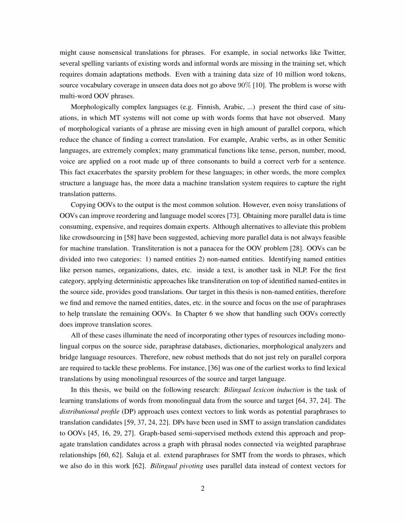
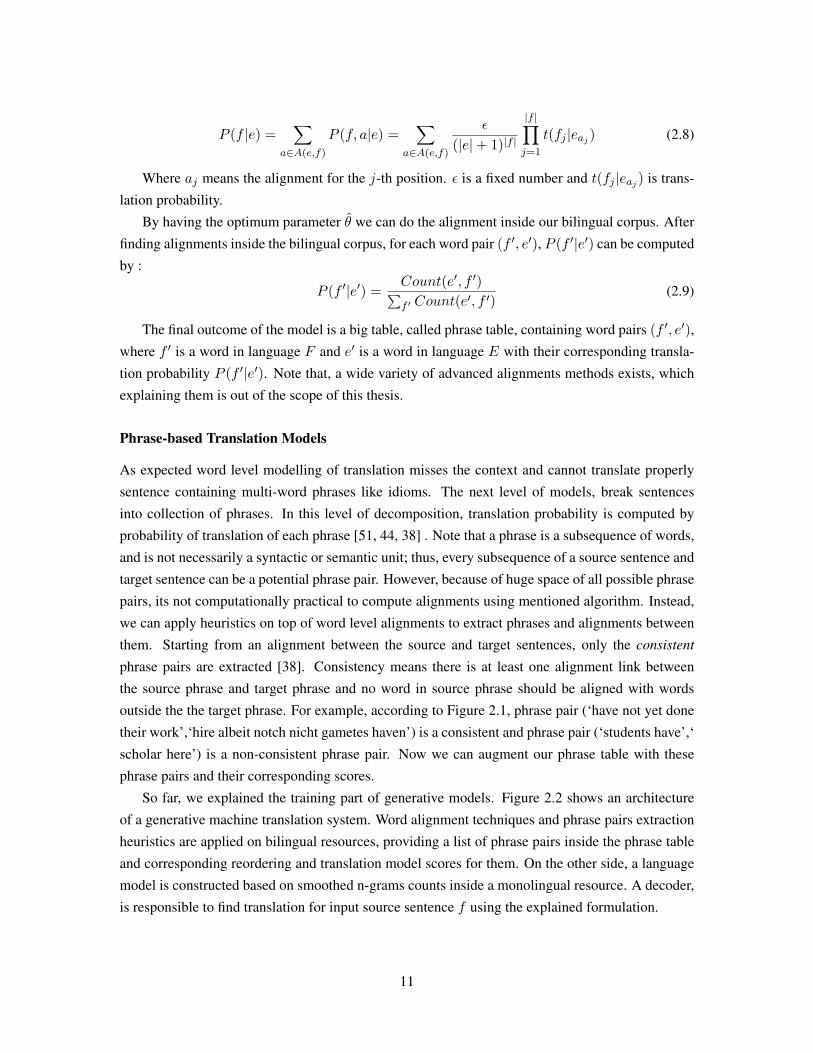
So far, we explained the training part of generative models. Figure 2.2 shows an architecture
of a generative machine translation system. Word alignment techniques and phrase pairs extraction
heuristics are applied on bilingual resources, providing a list of phrase pairs inside the phrase table
and corresponding reordering and translation model scores for them. On the other side, a language
model is constructed based on smoothed n-grams counts inside a monolingual resource. A decoder,
is responsible to find translation for input source sentence f using the explained formulation.
11
Translation ModelP(f | e)
Language ModelP(e)
source sentence
Monolingual resourceson target
N-gram countingSmoothing
target sentence
Reordering model
Bilingual resources
Word Alignment
phrase extraction
Phrase table
Phrase-based Decoder
Figure 2.2: Architecture of a generative machine translation system.
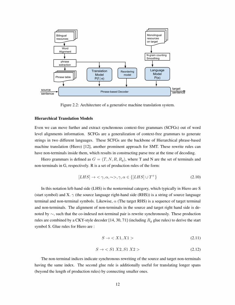
Hierarchical Translation Models
Even we can move further and extract synchronous context-free grammars (SCFGs) out of word
level alignments information. SCFGs are a generalization of context-free grammars to generate
strings in two different languages. These SCFGs are the backbone of Hierarchical phrase-based
machine translation (Hiero) [12], another prominent approach for SMT. These rewrite rules can
have non-terminals inside them, which results in constructing parse tree at the time of decoding.
Hiero grammars is defined as G = (T,N,R,Rg), where T and N are the set of terminals and
non-terminals in G, respectively. R is a set of production rules of the form:
[LHS]→ < γ, α,∼>, γ, α ∈ {[LHS] ∪ T+} (2.10)
In this notation left-hand side (LHS) is the nonterminal category, which typically in Hiero are S
(start symbol) and X. γ (the source language right-hand side (RHS)) is a string of source language
terminal and non-terminal symbols. Likewise, α (The target RHS) is a sequence of target terminal
and non-terminals. The alignment of non-terminals in the source and target right hand side is de-
noted by ∼, such that the co-indexed not-terminal pair is rewrite synchronously. These production
rules are combined by a CKY-style decoder [14, 30, 71] (including Rg glue rules) to derive the start
symbol S. Glue rules for Hiero are :
S → < X1, X1 > (2.11)
S → < S1 X2, S1 X2 > (2.12)
The non-terminal indices indicate synchronous rewriting of the source and target non-terminals
having the same index. The second glue rule is additionally useful for translating longer spans
(beyond the length of production rules) by connecting smaller ones.
12
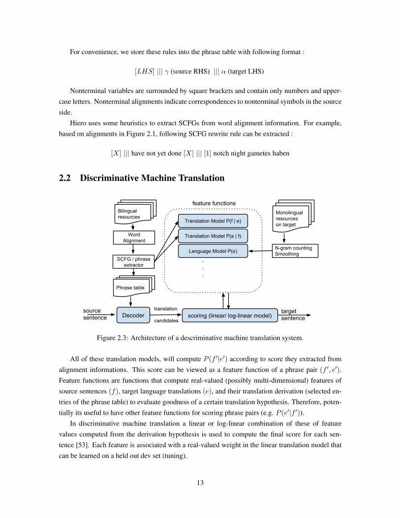
For convenience, we store these rules into the phrase table with following format :
[LHS] ||| γ (source RHS) ||| α (target LHS)
Nonterminal variables are surrounded by square brackets and contain only numbers and upper-
case letters. Nonterminal alignments indicate correspondences to nonterminal symbols in the source
side.
Hiero uses some heuristics to extract SCFGs from word alignment information. For example,
based on alignments in Figure 2.1, following SCFG rewrite rule can be extracted :
[X] ||| have not yet done [X] ||| [1] notch night gametes haben
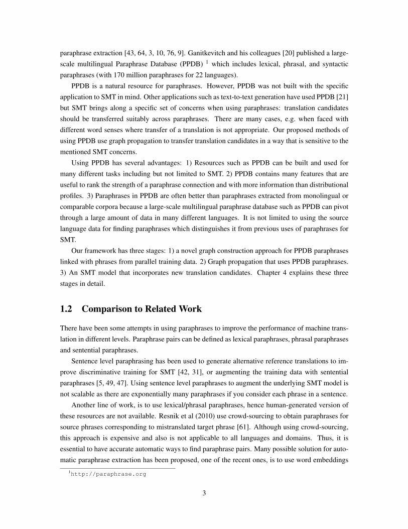
2.2 Discriminative Machine Translation
Translation Model P(f | e)
source sentence
Bilingual resources
Monolingual resourceson target
Word Alignment
N-gram countingSmoothing
target sentence
translation
candidatesDecoder
SCFG / phrase extractor
Phrase table
scoring (linear/ log-linear model)
feature functions
Translation Model P(e | f)
Language Model P(e)
.
.
.
Figure 2.3: Architecture of a descriminative machine translation system.
All of these translation models, will compute P (f ′|e′) according to score they extracted from
alignment informations. This score can be viewed as a feature function of a phrase pair (f ′, e′).
Feature functions are functions that compute real-valued (possibly multi-dimensional) features of
source sentences (f), target language translations (e), and their translation derivation (selected en-
tries of the phrase table) to evaluate goodness of a certain translation hypothesis. Therefore, poten-
tially its useful to have other feature functions for scoring phrase pairs (e.g. P (e′|f ′)).
In discriminative machine translation a linear or log-linear combination of these of feature
values computed from the derivation hypothesis is used to compute the final score for each sen-
tence [53]. Each feature is associated with a real-valued weight in the linear translation model that
can be learned on a held out dev set (tuning).
13
Previously we have explained the combination of generative translation model log probability
and target language model log probability for finding the best translation. In this framework these
two are also considered as features. Standard feature functions in this framework are conditional
translation probabilities p(e|f) and p(f |e), conditional lexical weights plex(e|f) and plex(f |e),
phrase penalty, word penalty, glue rule weight and language model.
An standard statistical model of SMT (Hiero) [53] uses a log linear model to score each possible
Hiero derivation in terms of different feature functions as :
P (derivation) ∝ (k−1∏i=1
∏r∈Rd
Φi(r)wi)Plm(e)wk (2.13)
where k is the total number of features and wi denote the weights of the feature function Φi. The
LM feature is the k-th feature which computed for the target sentence. While other features are
computed for each rule r that is used in derivation. These feature weights can be optimized with
respect to an automatic evaluation metric.
2.3 Evaluation of MT Systems
Human quality judgment is a good measure to evaluate the output of machine translation but its
subjective, time consuming, expensive, and sometimes tough because of ambiguity. An automatic
evaluation metric for machine translation is a must; hence it is still an open challenge. The root
of difficulty of automatic evaluation is the fact that there is no gold standard translation output for
each input sentence. Even a sentence in the source language might have many correct translations
which are different in structure and words. Among many possible measures have been proposed,
some of them are more common and preferred by researchers in this line of research. These metrics
evaluate the quality of SMT-generated translation relative to one or more human-generated reference
translation.
BLEU The bilingual evaluation understudy (BLEU) score is geometric mean of n-gram precisions
that is scaled by a brevity penalty to prevent very short sentences with some matching material
from being given inappropriately high scores [57].
TER Translation Edit Rate (TER) measures the amount of editing that a human would have to
perform to change a system output so it exactly matches a reference translation [65].
METEOR is an automatic metric for machine translation evaluation that is based on a general-
ized concept of unigram matching between the machine-produced translation and human-
produced reference translations. Unigrams can be matched based on their surface forms,
stemmed forms, and meanings; furthermore, METEOR can be easily extended to include
more advanced matching strategies [2].
Linear combinations of these metrics has shown promising results recently [63].
14
In this thesis, we have selected to use BLEU score [57] for automatic evaluating machine trans-
lation quality; since it is the most trusted measure and it does not require any type of external
resources like METEOR.
2.4 Semi-Supervised Learning (SSL)
Most of famous supervised machine learning methods have some mechanism to avoid overfitting;
Support Vector Machine (SVM) maximize the margin to data instances, Maximum Entropy (Max-
Ent) models try to minimize the risk of unpredictable data instances. Hence, most of these methods
relay on the availability of a good labeled slice of the whole data instances.
Another line of works that recently became a hot topic, is the usage of unlabeled data along-
side labeled data known as Semi-Supervised Learning (SSL). Collecting huge amount of unlabeled
data is cheaper, faster and sometimes more effective than labeling instances in small portion. For
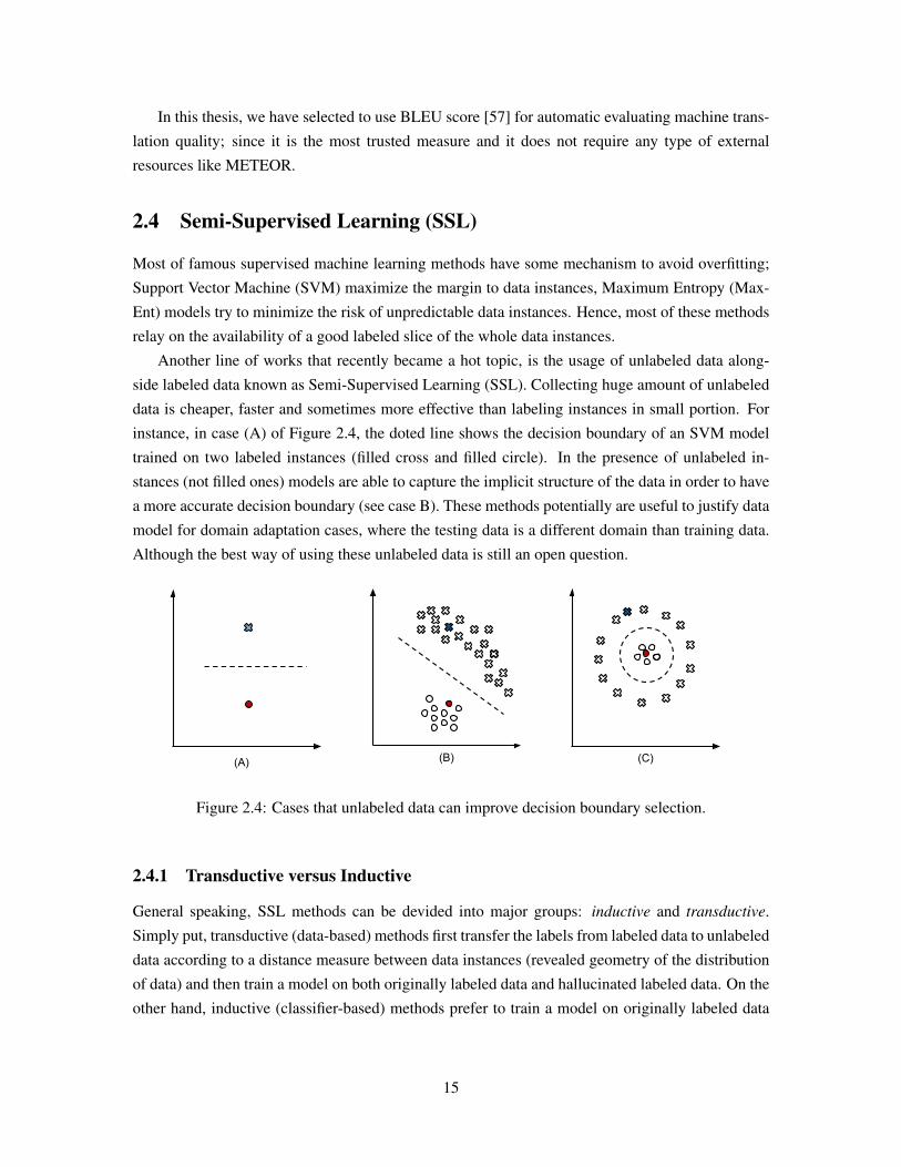
instance, in case (A) of Figure 2.4, the doted line shows the decision boundary of an SVM model
trained on two labeled instances (filled cross and filled circle). In the presence of unlabeled in-
stances (not filled ones) models are able to capture the implicit structure of the data in order to have
a more accurate decision boundary (see case B). These methods potentially are useful to justify data
model for domain adaptation cases, where the testing data is a different domain than training data.
Although the best way of using these unlabeled data is still an open question.
(A) (B) (C)
Figure 2.4: Cases that unlabeled data can improve decision boundary selection.
2.4.1 Transductive versus Inductive
General speaking, SSL methods can be devided into major groups: inductive and transductive.
Simply put, transductive (data-based) methods first transfer the labels from labeled data to unlabeled
data according to a distance measure between data instances (revealed geometry of the distribution
of data) and then train a model on both originally labeled data and hallucinated labeled data. On the
other hand, inductive (classifier-based) methods prefer to train a model on originally labeled data
15
and then use their model to predict the label for unlabeled data and gradually produce new training
data by injecting (noisy) labels to unlabeled data, and iteratively learn new classifier(s).
Whether to select transductive methods rather than inductive ones are an open discussion be-
tween researchers, and there are some cases that one of them fails. Case (c) in Figure 2.4 shows one
of cases that inductive methods might fail to fit properly.
2.4.2 Graph Based methods
Transferring the labels between data instances is another view for classifying these methods. One
of the most preferred methods is to use a graph structure between data instances and transfer labels
based on their distance in graph. Graph based methods have some advantageous: 1) In many cases
the unlabeled data are naturally expressed in a graph structure (e.g. social network information), 2)
they show more flexibility to be scalable, because of research going on parallelize graph processing,
3) many tools and frameworks have been developed to work with graphs [66]. Scalability is an
important concern when using semi-supervised methods, since most of them are non-parametric
(i.e. number of parameters grows with data size).
In graph-based transductive methods, a graph is constructed using a similarity measure defined
between data instances, then transferring labels occurs based on smoothness assumption. Smooth-
ness assumption implies that if two instances (nodes in the graph) are similar then the output la-
bels for them should be similar. Note that meaning of similarity is highly correlated on the task,
therefore, there is no big graph available for all machine learning techniques and creating a graph
according to each task is a critical step in these methods.
We built a graph of source language phrases and according to our task (machine translation),
we considered the relationship between nodes (phrases), to be paraphrase of each other. If two
nodes are paraphrase of each other, they should be close to each other in the graph. For each
node we have a distribution over labels. Labels in our graph are translations of a phrase (node)
in the target language. Therefore, for each source phrase inside the graph we have a distribution
of possible translations. Paraphrases are phrases which share the same meaning but expressed in
different words and structure; which is totally in harmony of our task. We would like to transfer the
translation from labeled nodes to unlabeled nodes and then train a SMT.
2.5 Summary
In this chapter, we reviewed all the background knowledge needed to follow the rest of the the-
sis, including: Phrase-based Statistical Machine Translation, Hierarchical Machine Translation and
Semi-supervised Learning.
16
Chapter 3
Automatic Paraphrase ExtractionMethods
Our goal is to produce translations for OOV phrases by exploiting paraphrases from the multilingual
PPDB [20] and by using graph propagation. Since our approach relies on phrase-level paraphrases
we compare with the current state of the art approaches that use monolingual data and distributional
profiles to construct paraphrases and use graph propagation [60, 62].
3.1 Paraphrases from Distributional Profiles
A distributional profile (DP) of a word or phrase was first proposed in [59] for SMT. Given a word
f , its distributional profile is:
DP (f) = {〈A(f, wi)〉 | wi ∈ V }
V is the vocabulary and the surrounding words wi are taken from a monolingual corpus using a
fixed window size. We use a window size of 4 words based on the experiments in [60]. The counts
of words in the surrounding context can be positional or non-positional. Following [60], we use
non-positional counts to alleviate sparsity problem. DPs need an association measure A(·, ·) to
compute distances between potential paraphrases. A comparison of different association measures
appears in [45, 60, 62] and our preliminary experiments validated the choice of the same association
measure as in these papers, namely Point-wise Mutual Information [40] (PMI). For each potential
context word wi:
PMI(f, wi) = log2P (f, wi)P (f)P (wi)
(3.1)
Positive values of PMI shows that under standard independence assumptions, the given words co-
occur more than what we expect [40]. We refer to PMI using the notation A(·, ·). To evaluate the
similarity between two phrases we use cosine similarity. The cosine coefficient of two phrases f1
17
and f2 is:
S(f1, f2) = cos(DP (f1), DP (f2)) =∑wi∈V A(f1, wi)A(f2, wi)√∑
wi∈V A(f1, wi)2√∑
wi∈V A(f2, wi)2
(3.2)
where V is the vocabulary. Note that in Eqn. (3.2) wi’s are the words that appear in the context of
f1 or f2, otherwise the PMI values would be zero.
Considering all possible candidate paraphrases is very expensive. Thus, we use the heuristic
applied in previous works [45, 60, 62] to reduce the search space. For each phrase we just keep
candidate paraphrases which appear in one of the surrounding context (e.g. Left Right) among all
occurrences of the phrase.
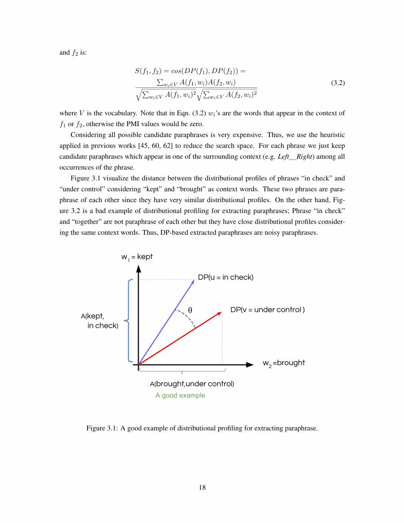
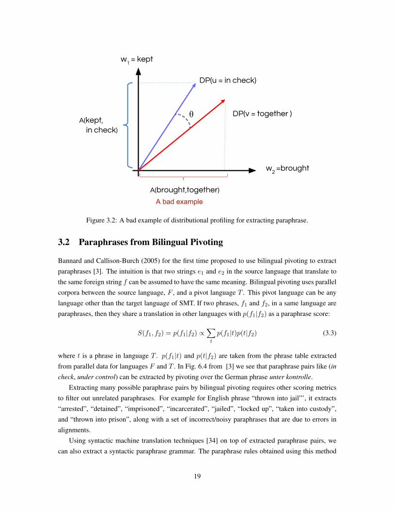
Figure 3.1 visualize the distance between the distributional profiles of phrases “in check” and
“under control” considering “kept” and “brought” as context words. These two phrases are para-
phrase of each other since they have very similar distributional profiles. On the other hand, Fig-
ure 3.2 is a bad example of distributional profiling for extracting paraphrases; Phrase “in check”
and “together” are not paraphrase of each other but they have close distributional profiles consider-
ing the same context words. Thus, DP-based extracted paraphrases are noisy paraphrases.
A(kept,
in check)
A(brought,under control)
w1
= kept
w2
=brought
DP(u = in check)
DP(v = under control ) θ
A good example
Figure 3.1: A good example of distributional profiling for extracting paraphrase.
18
A(kept,
in check)
A(brought,together)
w1
= kept
w2
=brought
DP(u = in check)
DP(v = together ) θ
in |V| dimensional space
A bad example
Figure 3.2: A bad example of distributional profiling for extracting paraphrase.
3.2 Paraphrases from Bilingual Pivoting
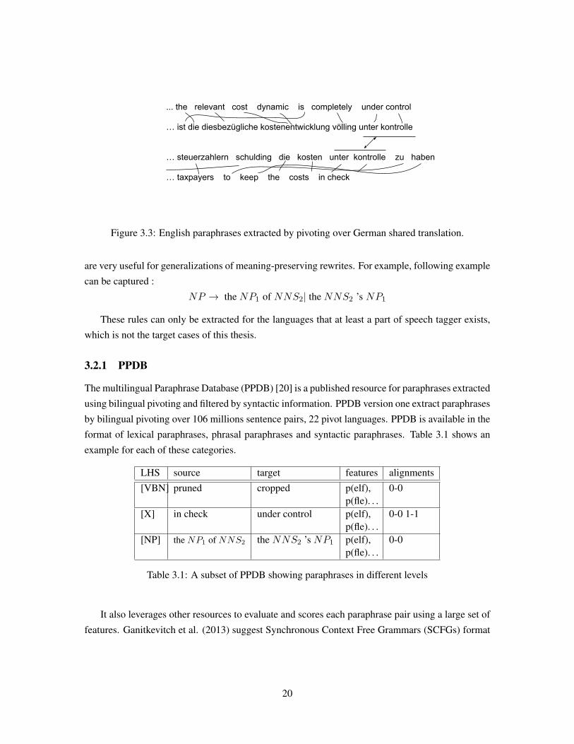
Bannard and Callison-Burch (2005) for the first time proposed to use bilingual pivoting to extract
paraphrases [3]. The intuition is that two strings e1 and e2 in the source language that translate to
the same foreign string f can be assumed to have the same meaning. Bilingual pivoting uses parallel
corpora between the source language, F , and a pivot language T . This pivot language can be any
language other than the target language of SMT. If two phrases, f1 and f2, in a same language are
paraphrases, then they share a translation in other languages with p(f1|f2) as a paraphrase score:
S(f1, f2) = p(f1|f2) ∝∑
t
p(f1|t)p(t|f2) (3.3)
where t is a phrase in language T . p(f1|t) and p(t|f2) are taken from the phrase table extracted
from parallel data for languages F and T . In Fig. 6.4 from [3] we see that paraphrase pairs like (in
check, under control) can be extracted by pivoting over the German phrase unter kontrolle.
Extracting many possible paraphrase pairs by bilingual pivoting requires other scoring metrics
to filter out unrelated paraphrases. For example for English phrase “thrown into jail”’, it extracts
“arrested”, “detained”, “imprisoned”, “incarcerated”, “jailed”, “locked up”, “taken into custody”,
and “thrown into prison”, along with a set of incorrect/noisy paraphrases that are due to errors in
alignments.
Using syntactic machine translation techniques [34] on top of extracted paraphrase pairs, we
can also extract a syntactic paraphrase grammar. The paraphrase rules obtained using this method
19
... the relevant cost dynamic is completely under control
… ist die diesbezügliche kostenentwicklung völling unter kontrolle
… steuerzahlern schulding die kosten unter kontrolle zu haben
… taxpayers to keep the costs in check
Figure 3.3: English paraphrases extracted by pivoting over German shared translation.
are very useful for generalizations of meaning-preserving rewrites. For example, following example
can be captured :
NP → the NP1 of NNS2| the NNS2 ’s NP1
These rules can only be extracted for the languages that at least a part of speech tagger exists,
which is not the target cases of this thesis.
3.2.1 PPDB
The multilingual Paraphrase Database (PPDB) [20] is a published resource for paraphrases extracted
using bilingual pivoting and filtered by syntactic information. PPDB version one extract paraphrases
by bilingual pivoting over 106 millions sentence pairs, 22 pivot languages. PPDB is available in the
format of lexical paraphrases, phrasal paraphrases and syntactic paraphrases. Table 3.1 shows an
example for each of these categories.
LHS source target features alignments[VBN] pruned cropped p(elf),
p(fle). . .0-0
[X] in check under control p(elf),p(fle). . .
0-0 1-1
[NP] the NP1 of NNS2 the NNS2 ’s NP1 p(elf),p(fle). . .
0-0
Table 3.1: A subset of PPDB showing paraphrases in different levels
It also leverages other resources to evaluate and scores each paraphrase pair using a large set of
features. Ganitkevitch et al. (2013) suggest Synchronous Context Free Grammars (SCFGs) format
20
to store paraphrase relationship in paraphrase databases.
LHS ||| source ||| target ||| (feature = value)∗ ||| alignment
For example :
[V BN ] ||| pruned ||| cropped ||| p(e|f) = 4.33, p(f |e) = 4.88 . . . ||| 0− 0
This format allows us to store additional feature scores for each paraphrase pair, since there are
various ways to estimate score S(f1, f2). These features can also contains monolingual information
like the scores from the previous technique, which we found very useful.
LHS source target features alignment[NN] issue matter p(elf) xW1+
p(fle) xW2+Lex(fle) xW3+Lex(elf) xW4+p(elf,LHS) xW5+GoogleNgram-Sim xW6+. . .
0-0
= score(issue,matter)
Table 3.2: Scoring paraphrase pairs by linear combination of features inside the PPDB
These features can be used by a log linear model to score paraphrases [76]. We used a linear
combination of these features using the equation in Sec. 3 of [20] to score each paraphrase pair (see
Table 3.2). PPDB version 1 is broken into different levels of coverage. The smaller sizes contain
only better-scoring, high-precision paraphrases, while larger sizes aim for high coverage. Table 3.3
shows number of rules available inside English PPDB for each size divided into different categories.
Size lexical one-to-many phrasal syntacticS 31K 47K 637K 585KM 69K 94K 1.2M 1.0ML 198K 188K 3.0M 2.2MXL 548K 376K 6.9M 4.4MXXL 2.1M 752K 29.2M 9.3MXXXL 7.6M 1.5M 68.4M 16.1M
Table 3.3: English PPDB version 1 statistics (number of rules)
21
3.3 Summary
We describe two major methods for automatically acquiring paraphrase pairs, then we introduce
PPDB, a multi-lingual paraphrase database, and its desirable properties. We have chosen PPDB as
a paraphrase database for the rest of this work because of the following reasons:
• DP-based paraphrases are noisy in compare to bilingual pivoted extracted paraphrases
• Computing distributional profile for n-grams higher than bigrams is computationally intractable
• PPDB provides many features for each paraphrase pair including features extracted from
monolingual resources.
In chapter 6 we examine DP-based paraphrases in compare to PPDB paraphrases in the task of
machine translation.
22
Chapter 4
Methodology
4.1 Overview
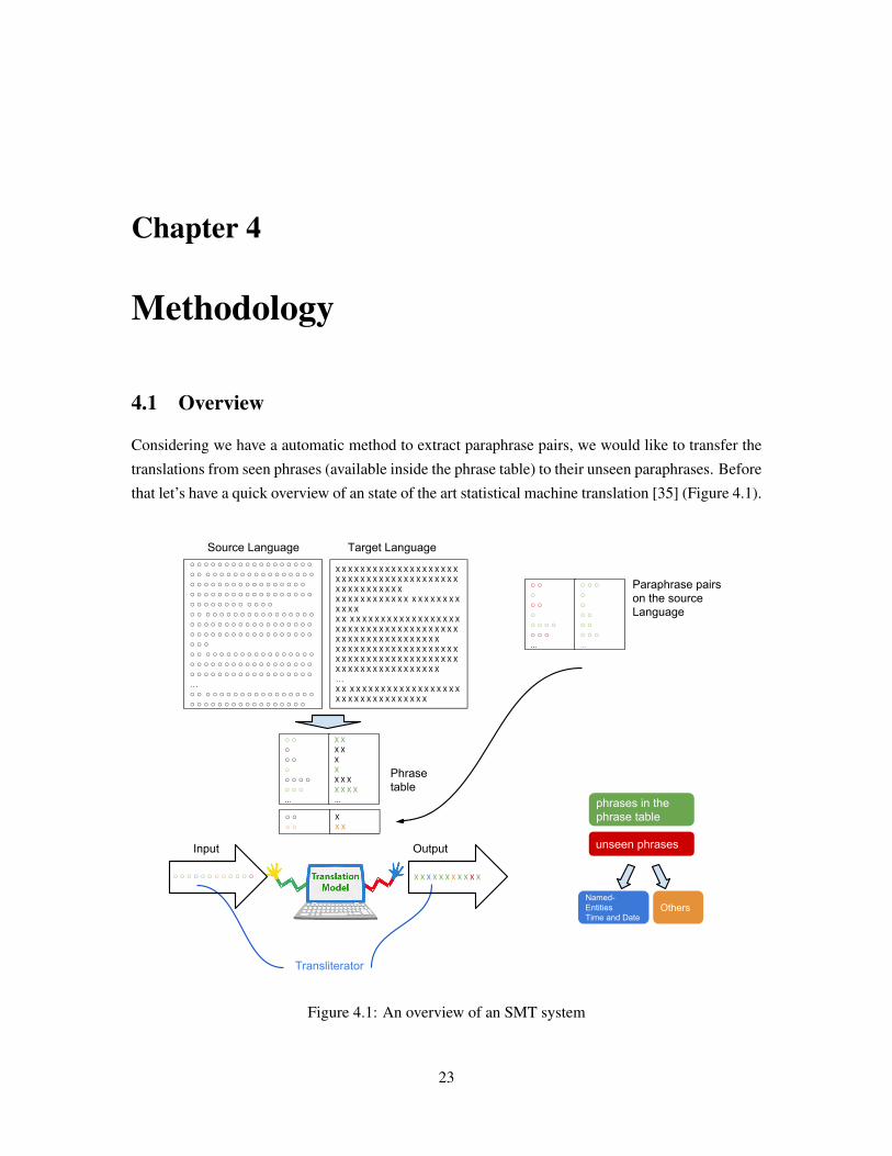
Considering we have a automatic method to extract paraphrase pairs, we would like to transfer the
translations from seen phrases (available inside the phrase table) to their unseen paraphrases. Before
that let’s have a quick overview of an state of the art statistical machine translation [35] (Figure 4.1).
○ ○ ○ ○ ○ ○ ○ ○ ○ ○ ○ ○ ○ ○ ○ ○ ○ ○ ○ ○ ○ ○ ○ ○ ○ ○ ○ ○ ○ ○ ○ ○ ○ ○ ○ ○ ○ ○ ○ ○ ○ ○ ○ ○ ○ ○ ○ ○ ○ ○ ○ ○ ○ ○ ○ ○ ○ ○ ○ ○ ○ ○ ○ ○ ○ ○ ○ ○ ○ ○ ○ ○ ○ ○ ○ ○ ○ ○ ○ ○ ○ ○ ○ ○ ○ ○ ○ ○ ○ ○ ○ ○ ○ ○ ○ ○ ○ ○ ○ ○ ○ ○ ○ ○ ○ ○ ○ ○ ○ ○ ○ ○ ○ ○ ○ ○ ○ ○ ○ ○ ○ ○ ○ ○ ○ ○ ○ ○ ○ ○ ○ ○ ○ ○ ○ ○ ○ ○ ○ ○○ ○ ○ ○ ○ ○ ○ ○ ○ ○ ○ ○ ○ ○ ○ ○ ○ ○ ○ ○ ○ ○ ○ ○ ○ ○ ○ ○ ○ ○ ○ ○ ○ ○ ○ ○ ○ ○ ○ ○ ○ ○ ○ ○ ○ ○ ○ ○ ○ ○ ○ ○ ○ ○ …○ ○ ○ ○ ○ ○ ○ ○ ○ ○ ○ ○ ○ ○ ○ ○ ○ ○ ○ ○ ○ ○ ○ ○ ○ ○ ○ ○ ○ ○ ○ ○ ○ ○ ○
X X X X X X X X X X X X X X X X X X X X X X X X X X X X X X X X X X X X X X X X X X X X X X X X X X X X X X X X X X X X X X X X X X X X X X X X X X X X X X X X X X X X X X X X X X X X X X X X X X X X X X X X X X X X X X X X X X X X X X X X X X X X X X X X X X X XX X X X X X X X X X X X X X X X X X X X X X X X X X X X X X X X X X X X X X X X X X X X X X X X X X X X X X X X X …X X X X X X X X X X X X X X X X X X X X X X X X X X X X X X X X X X X
Source Language Target Language
○ ○ ○ ○ ○ ○ ○ ○ ○ ○ ○ ○ ○ ...
X X X X XX X X X X X X X...
Phrase table
○ ○ ○ ○ ○ ○ ○ ○ ○ ○ ○ ○ ○ ...
○ ○ ○○ ○ ○ ○○ ○ ○ ○ ○ ...
Paraphrase pairson the source Language
Input
○ ○ ○ ○ ○ ○ ○ ○ ○ ○ ○ ○ X X X X X X X X X X X
Output
Transliterator
Input
○ ○ ○ ○ ○ ○ ○ ○ ○ ○ ○ ○ X X X X X X X X X X X
Output unseen phrases
phrases in the phrase table
Named-Entities Time and Date
Others
○ ○ ○ ○
X X X
Figure 4.1: An overview of an SMT system
23
For translating from a source language to a target language a bilingual parallel corpus is re-
quired. According to translation patterns inside the parallel sentence a phrase table can be extracted
which later on used by a translation system. Translation system tries to search for the phrases of
any input sentence inside the phrase table. Not surprising, some of these phrases are not available
inside the phrase table (shown by red color), which we call it OOV phrases. A group of these OOV
phrases are Named-Entities, which can be translated using a transliterator [32]. Even if we remove
these Named-Entities, there still a huge collection of unseen phrases missing inside the phrase table.
We want to use a paraphrase database to transfer the translation from seen phrase to their unseen
paraphrases and augment the phrase table with these new translation. These new translations can
potentially increase the OOV coverage at the test time. The remaining question is how to transfer
these translations.
4.2 Transferring Translations
4.2.1 Naive Approach
A naive approach for transferring the translation is to use the following formulation :
P (translation|unseen phrase) =∑
para ∈ { paraphrases }
P (translation|para) · P (para|unseen phrase)
In this formulation we pivot over paraphrases and multiple paraphrase probability and translation
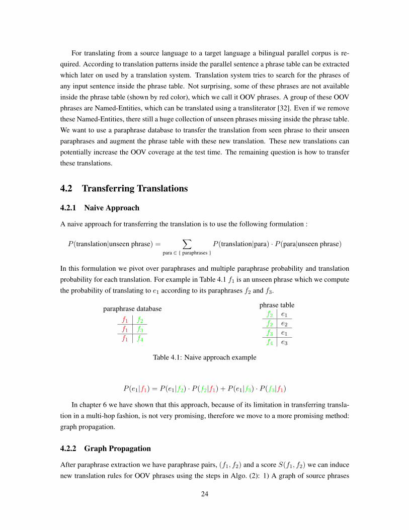
probability for each translation. For example in Table 4.1 f1 is an unseen phrase which we compute
the probability of translating to e1 according to its paraphrases f2 and f3.
paraphrase databasef1 f2f1 f3f1 f4
phrase tablef2 e1f2 e2f3 e1f4 e3
Table 4.1: Naive approach example
P (e1|f1) = P (e1|f2) · P (f2|f1) + P (e1|f3) · P (f3|f1)
In chapter 6 we have shown that this approach, because of its limitation in transferring transla-
tion in a multi-hop fashion, is not very promising, therefore we move to a more promising method:
graph propagation.
4.2.2 Graph Propagation
After paraphrase extraction we have paraphrase pairs, (f1, f2) and a score S(f1, f2) we can induce
new translation rules for OOV phrases using the steps in Algo. (2): 1) A graph of source phrases
24
Algorithm 2 PPDB Graph Propagation for SMTPhrTable = PhraseTableGeneration();ParaDB = ParaphraseExtraction(); (Sec. 3)InitGraph = GraphConstruct(PhrTable, ParaDB); (Sec. 4.2.2)PropGraph = GraphPropagation(InitGraph); (Sec. 4.2.2)for phrase ∈ {OOVs} do
newTrans = TranslationFinder(PropGraph, phrase);Augment(PhrTable, newTrans); (Sec. 4.3)
TuneMT(PhrTable);
Size Nodes Edges MaxNeigh.
AveNeigh.
S 23K 31K 32 1.38M 41K 69K 33 1.69L 74K 199K 67 2.69XL 103K 548K 330 5.33XXL 122K 2073K 1231 16.968XXXL 125K 7558K 5255 60.27
Table 4.2: Statistics of the graph constructed using the English lexical PPDB
is constructed as in [60]; containing both sides of paraphrase pairs and source side of phrase table;
2) translations are propagated as labels through the graph as explained in Fig. 4.6; and 3) new
translation rules obtained from graph-propagation are integrated with the original phrase table.
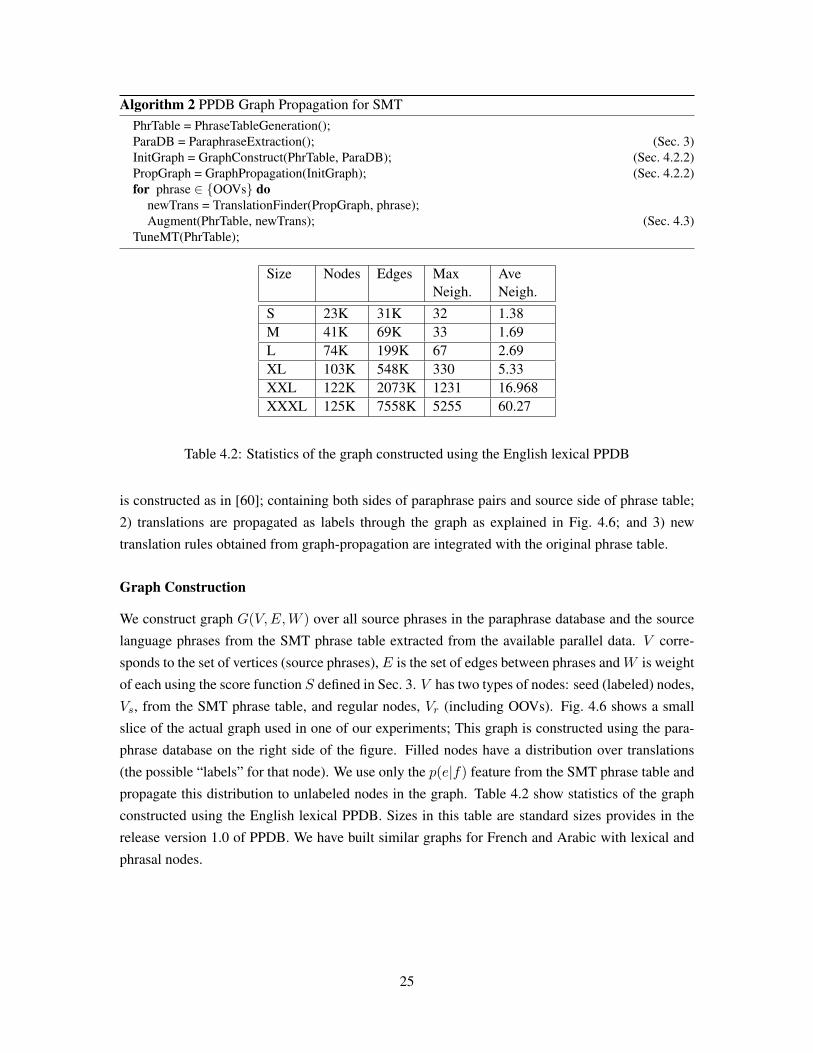
Graph Construction
We construct graph G(V,E,W ) over all source phrases in the paraphrase database and the source
language phrases from the SMT phrase table extracted from the available parallel data. V corre-
sponds to the set of vertices (source phrases), E is the set of edges between phrases andW is weight
of each using the score function S defined in Sec. 3. V has two types of nodes: seed (labeled) nodes,
Vs, from the SMT phrase table, and regular nodes, Vr (including OOVs). Fig. 4.6 shows a small
slice of the actual graph used in one of our experiments; This graph is constructed using the para-
phrase database on the right side of the figure. Filled nodes have a distribution over translations
(the possible “labels” for that node). We use only the p(e|f) feature from the SMT phrase table and
propagate this distribution to unlabeled nodes in the graph. Table 4.2 show statistics of the graph
constructed using the English lexical PPDB. Sizes in this table are standard sizes provides in the
release version 1.0 of PPDB. We have built similar graphs for French and Arabic with lexical and
phrasal nodes.
25
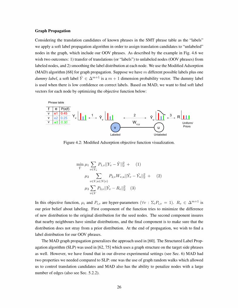
Graph Propagation
Considering the translation candidates of known phrases in the SMT phrase table as the “labels”
we apply a soft label propagation algorithm in order to assign translation candidates to “unlabeled”
nodes in the graph, which include our OOV phrases. As described by the example in Fig. 4.6 we
wish two outcomes: 1) transfer of translations (or “labels”) to unlabeled nodes (OOV phrases) from
labeled nodes, and 2) smoothing the label distribution at each node. We use the Modified Adsorption
(MAD) algorithm [68] for graph propagation. Suppose we havem different possible labels plus one
dummy label, a soft label Y ∈ ∆m+1 is a m + 1 dimension probability vector. The dummy label
is used when there is low confidence on correct labels. Based on MAD, we want to find soft label
vectors for each node by optimizing the objective function below:
v uWv,u
Labeled
Phrase table
Unlabeled
f e P(e|f)
vvv
e1 0.45e2 0.25e3 0.30
ŶvYv Ŷu
RUniform/ Priors
1 32
Figure 4.2: Modified Adsorption objective function visualization.
minY
µ1∑
v∈Vs
P1,v||Yv − Y ||22 + (1)
µ2∑
v∈V,u∈N(v)P2,vWv,u||Yv − Yu||22 + (2)
µ3∑v∈V
P3,v||Yv −Rv||22 (3)
In this objective function, µi and Pi,v are hyper-parameters (∀v : ΣiPi,v = 1). Rv ∈ ∆m+1 is
our prior belief about labeling. First component of the function tries to minimize the difference
of new distribution to the original distribution for the seed nodes. The second component insures
that nearby neighbours have similar distributions, and the final component is to make sure that the
distribution does not stray from a prior distribution. At the end of propagation, we wish to find a
label distribution for our OOV phrases.
The MAD graph propagation generalizes the approach used in [60]. The Structured Label Prop-
agation algorithm (SLP) was used in [62, 75] which uses a graph structure on the target side phrases
as well. However, we have found that in our diverse experimental settings (see Sec. 6) MAD had
two properties we needed compared to SLP: one was the use of graph random walks which allowed
us to control translation candidates and MAD also has the ability to penalize nodes with a large
number of edges (also see Sec. 5.2.2).
26
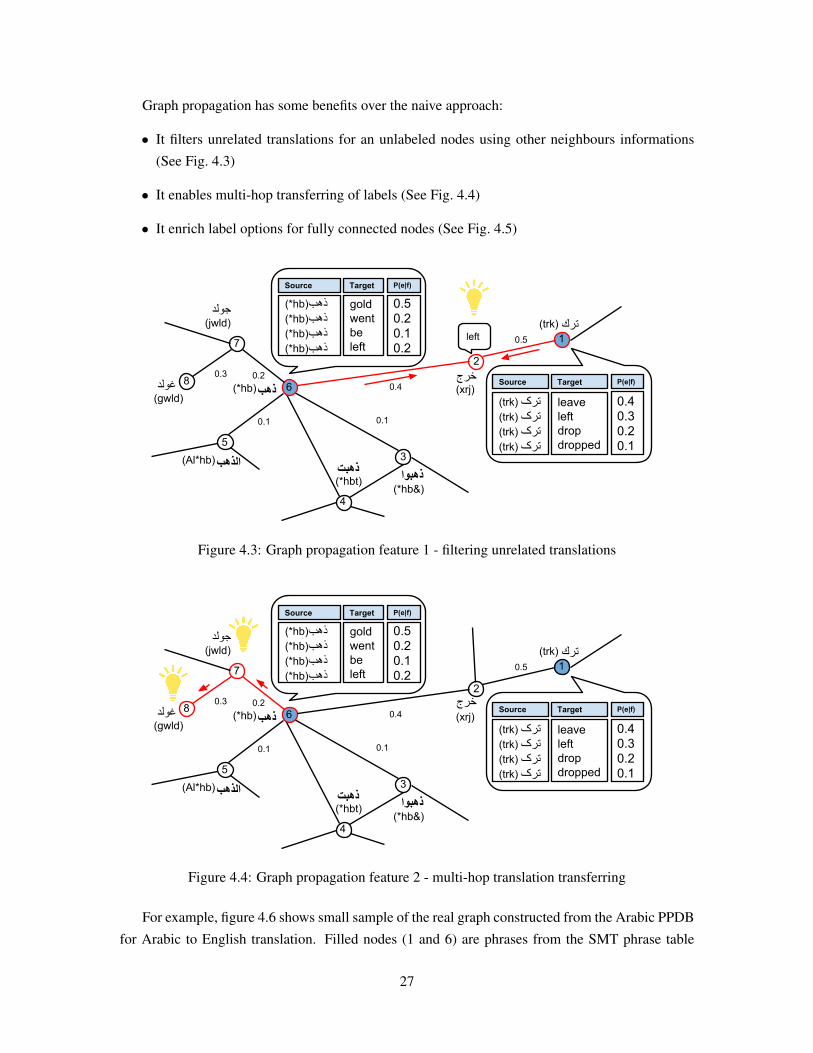
Graph propagation has some benefits over the naive approach:
• It filters unrelated translations for an unlabeled nodes using other neighbours informations
(See Fig. 4.3)
• It enables multi-hop transferring of labels (See Fig. 4.4)
• It enrich label options for fully connected nodes (See Fig. 4.5)
2
8
7
3
4
ذھبت
ذھب
ترك
ذھبوا
جولد
غولد
(trk)
(xrj)
(jwld)
(gwld)(*hb)
(*hb&)(*hbt)
1
6
5(Al*hb)الذھب
0.3خرج 0.2
0.1 0.1
0.4
0.5
(*hb)ذھب(*hb)ذھب(*hb)ذھب(*hb)ذھب
goldwent be left
0.50.2 0.1 0.2
Source Target P(e|f)
(trk) ترک(trk) ترک(trk) ترک(trk) ترک
Source
leaveleftdropdropped
0.40.3 0.2 0.1
Target P(e|f)
left
Figure 4.3: Graph propagation feature 1 - filtering unrelated translations
8
7
3
4
ذھبت
ذھب
ترك
ذھبوا
جولد
غولد
(trk)
(xrj)
(jwld)
(gwld)(*hb)
(*hb&)(*hbt)
2
1
6
5(Al*hb)الذھب
0.3خرج 0.2
0.1 0.1
0.4
0.5
(*hb)ذھب(*hb)ذھب(*hb)ذھب(*hb)ذھب
goldwent be left
0.50.2 0.1 0.2
Source Target P(e|f)
(trk) ترک(trk) ترک(trk) ترک(trk) ترک
Source
leaveleftdropdropped
0.40.3 0.2 0.1
Target P(e|f)
Figure 4.4: Graph propagation feature 2 - multi-hop translation transferring
For example, figure 4.6 shows small sample of the real graph constructed from the Arabic PPDB
for Arabic to English translation. Filled nodes (1 and 6) are phrases from the SMT phrase table
27
ذھبت
ذھب
ترك
ذھبوا
جولد
غولد
3
(trk)
(xrj)
(jwld)
(gwld)(*hb)
(*hb&)(*hbt)
8
2
1
6
5(Al*hb)الذھب
4
خرج
7
0.3 0.2
0.1 0.1
0.4
0.5
(*hb)ذھب(*hb)ذھب(*hb)ذھب(*hb)ذھب
goldwent be left
0.50.2 0.1 0.2
Source Target P(e|f)
(trk) ترک(trk) ترک(trk) ترک(trk) ترک
Source
leaveleftdropdropped
0.40.3 0.2 0.1
Target P(e|f)
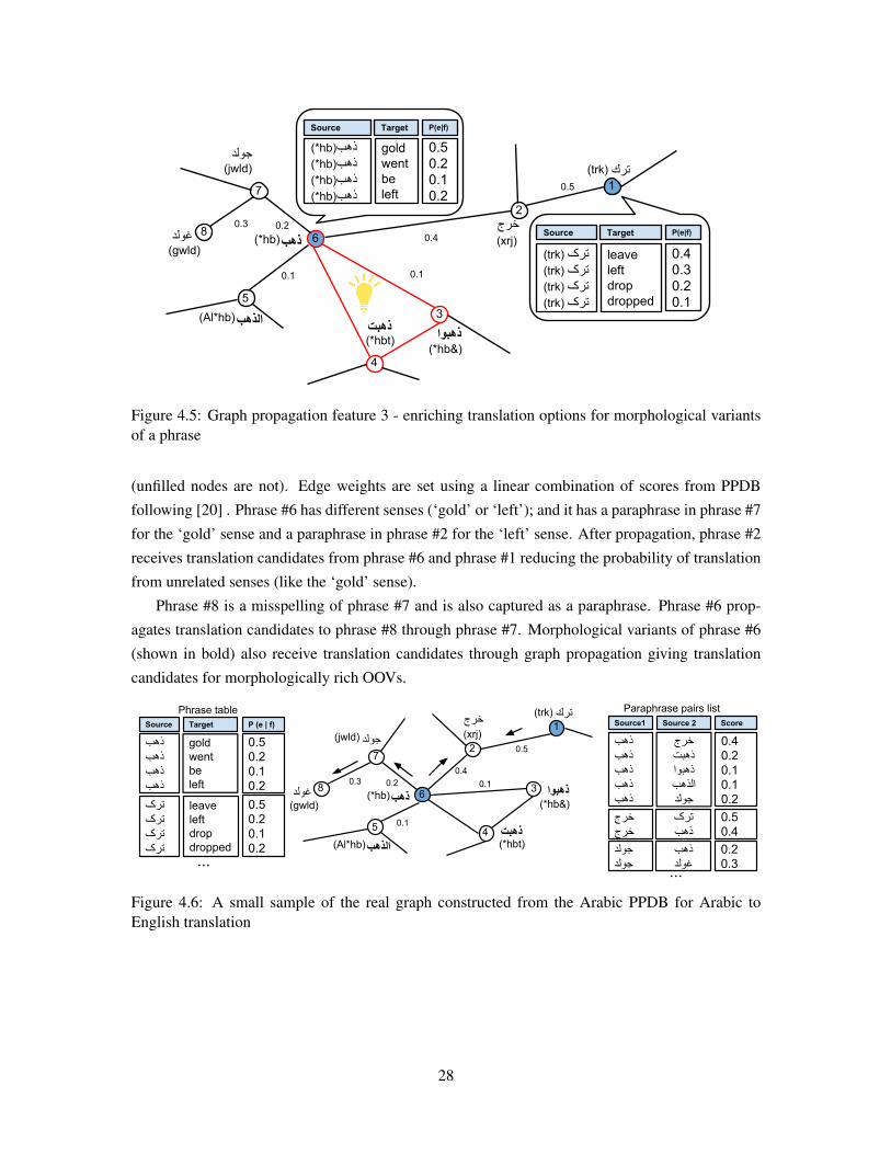
Figure 4.5: Graph propagation feature 3 - enriching translation options for morphological variantsof a phrase
(unfilled nodes are not). Edge weights are set using a linear combination of scores from PPDB
following [20] . Phrase #6 has different senses (‘gold’ or ‘left’); and it has a paraphrase in phrase #7
for the ‘gold’ sense and a paraphrase in phrase #2 for the ‘left’ sense. After propagation, phrase #2
receives translation candidates from phrase #6 and phrase #1 reducing the probability of translation
from unrelated senses (like the ‘gold’ sense).
Phrase #8 is a misspelling of phrase #7 and is also captured as a paraphrase. Phrase #6 prop-
agates translation candidates to phrase #8 through phrase #7. Morphological variants of phrase #6
(shown in bold) also receive translation candidates through graph propagation giving translation
candidates for morphologically rich OOVs.
خرج
ذھبت
ذھب
الذھب
ذھبذھبذھب ذھب
goldwent be left
ترکترکترکترک
Phrase table ترك
ذھبوا
جولد
غولد
Paraphrase pairs list
0.50.2 0.1 0.2
leaveleftdropdropped
0.50.2 0.1 0.2
Source Target P (e | f)
ذھبذھبذھبذھب ذھب
خرج ذھبت ذھبواالذھبجولد
0.40.2 0.1 0.1 0.2
Source1 Source 2 Score
خرجخرج
ترکذھب
0.50.4
جولدجولد
ذھبغولد
0.20.3...
0.40.2
0.5
0.10.3
0.1
...
1
2
3
4 5
6
7
8
(trk)
(xrj)(jwld)
(gwld)(*hb)
(Al*hb)
(*hb&)
(*hbt)
Figure 4.6: A small sample of the real graph constructed from the Arabic PPDB for Arabic toEnglish translation
28
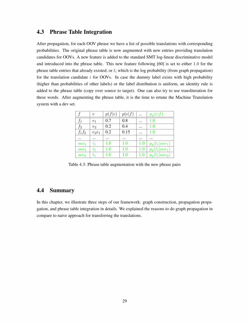
4.3 Phrase Table Integration
After propagation, for each OOV phrase we have a list of possible translations with corresponding
probabilities. The original phrase table is now augmented with new entries providing translation
candidates for OOVs. A new feature is added to the standard SMT log-linear discriminative model
and introduced into the phrase table. This new feature following [60] is set to either 1.0 for the
phrase table entries that already existed; or `i which is the log probability (from graph propagation)
for the translation candidate i for OOVs. In case the dummy label exists with high probability
(higher than probabilities of other labels) or the label distribution is uniform, an identity rule is
added to the phrase table (copy over source to target). One can also try to use transliteration for
these words. After augmenting the phrase table, it is the time to retune the Machine Translation
system with a dev set.
f e p(f |e) p(e|f) ... pg(e|f)f1 e1 0.7 0.8 ... 1.0f2 e2 0.2 0.4 ... 1.0f1f2 e2e1 0.2 0.15 ... 1.0... ... ... ... ... ...oov1 t1 1.0 1.0 1.0 pg(t1|oov1)oov1 t2 1.0 1.0 1.0 pg(t2|oov1)oov2 t1 1.0 1.0 1.0 pg(t1|oov2)
Table 4.3: Phrase table augmentation with the new phrase pairs
4.4 Summary
In this chapter, we illustrate three steps of our framework: graph construction, propagation propa-
gation, and phrase table integration in details. We explained the reasons to do graph propagation in
compare to naive approach for transferring the translations.
29
Chapter 5
Analysis of the Framework
5.1 Propagation of poor translations
Automatic paraphrase extraction generates many possible paraphrase candidates and many of them
are likely to be false positives for finding translation candidates for OOVs. Distributional profiles
rely on context information which is not sufficient to derive accurate paraphrases for many phrases
and this results in many low quality paraphrase candidates. For example, fruit names apple and
orange occur in similar context, but if we translate apple to naranja in Spanish, it conveys the
wrong meaning. Thus, filtering the paraphrase database by other resources like syntactic infor-
mation can be useful. Bilingual pivoting uses word alignments which can also introduce errors
depending on the size and quality of the bilingual data used. Alignment errors also introduce poor
translations. In graph propagation, these errors may be propagated and result in poor translations
for OOVs.
We could address this issue by aggressively pruning the potential paraphrase candidates to im-
prove the precision. However, this results in a dramatic drop in coverage and many OOV phrases do
not obtain any translation candidates. We use a combination of the following three steps to augment
our graph propagation framework.
5.1.1 Graph pruning and PPDB sizes
Pruning the graph avoids error propagation by removing unreliable edges. Pruning removes edges
with an edge weight lower than a minimum threshold (e- Neighbourhood) or by limiting the number
of neighbours to the top-K edges(K-NN) [67]. Each of these methods has their own advantageous
and disadvantageous. Figure 5.1 shows cases that K-NN will result in a asymmetric graph (case
A) or an irregular graph (Case B). On the other hand, e-neighbourhood method is very sensitive to
the value of e (i.e. this method can lead to disconnected components or uncultured structure) (see
Figure 5.2)
PPDB version 1 provides different sizes with different levels of accuracy and coverage. We can
do graph pruning simply by choosing to use different sizes of PPDB. As we can see in Fig. 5.3 results
30
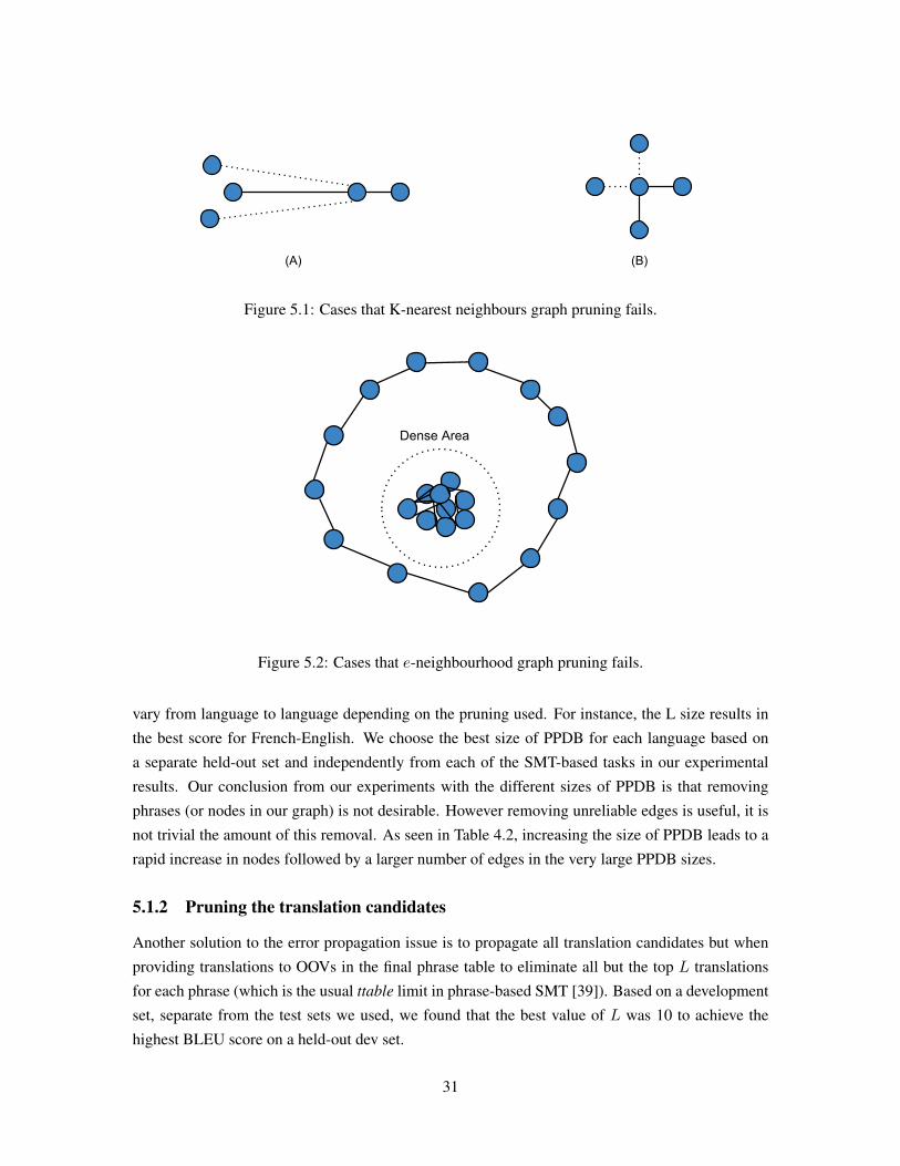
(A) (B)
Figure 5.1: Cases that K-nearest neighbours graph pruning fails.
Dense Area
Figure 5.2: Cases that e-neighbourhood graph pruning fails.
vary from language to language depending on the pruning used. For instance, the L size results in
the best score for French-English. We choose the best size of PPDB for each language based on
a separate held-out set and independently from each of the SMT-based tasks in our experimental
results. Our conclusion from our experiments with the different sizes of PPDB is that removing
phrases (or nodes in our graph) is not desirable. However removing unreliable edges is useful, it is
not trivial the amount of this removal. As seen in Table 4.2, increasing the size of PPDB leads to a
rapid increase in nodes followed by a larger number of edges in the very large PPDB sizes.
5.1.2 Pruning the translation candidates
Another solution to the error propagation issue is to propagate all translation candidates but when
providing translations to OOVs in the final phrase table to eliminate all but the top L translations
for each phrase (which is the usual ttable limit in phrase-based SMT [39]). Based on a development
set, separate from the test sets we used, we found that the best value of L was 10 to achieve the
highest BLEU score on a held-out dev set.
31
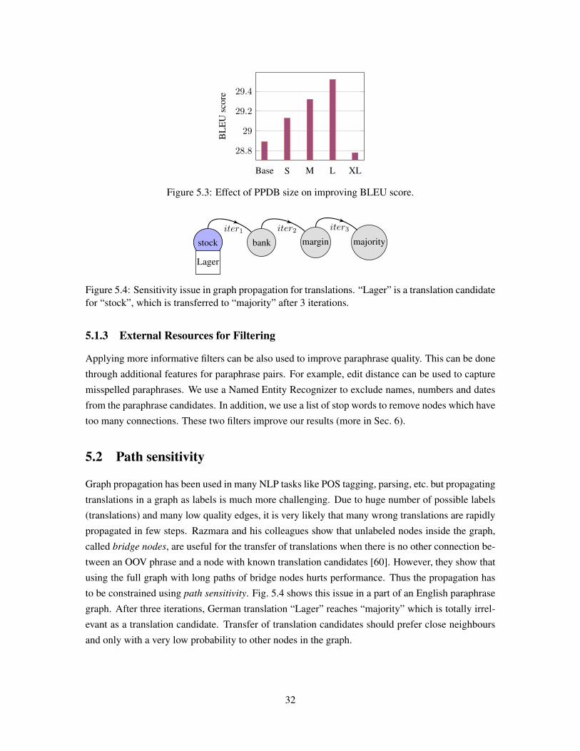
Base S M L XL
28.8
29
29.2
29.4
BL
EU
scor
e
Figure 5.3: Effect of PPDB size on improving BLEU score.
stock bank margin majoritystock
Lager
iter1 iter2 iter3
Figure 5.4: Sensitivity issue in graph propagation for translations. “Lager” is a translation candidatefor “stock”, which is transferred to “majority” after 3 iterations.
5.1.3 External Resources for Filtering
Applying more informative filters can be also used to improve paraphrase quality. This can be done
through additional features for paraphrase pairs. For example, edit distance can be used to capture
misspelled paraphrases. We use a Named Entity Recognizer to exclude names, numbers and dates
from the paraphrase candidates. In addition, we use a list of stop words to remove nodes which have
too many connections. These two filters improve our results (more in Sec. 6).
5.2 Path sensitivity
Graph propagation has been used in many NLP tasks like POS tagging, parsing, etc. but propagating
translations in a graph as labels is much more challenging. Due to huge number of possible labels
(translations) and many low quality edges, it is very likely that many wrong translations are rapidly
propagated in few steps. Razmara and his colleagues show that unlabeled nodes inside the graph,
called bridge nodes, are useful for the transfer of translations when there is no other connection be-
tween an OOV phrase and a node with known translation candidates [60]. However, they show that
using the full graph with long paths of bridge nodes hurts performance. Thus the propagation has
to be constrained using path sensitivity. Fig. 5.4 shows this issue in a part of an English paraphrase
graph. After three iterations, German translation “Lager” reaches “majority” which is totally irrel-
evant as a translation candidate. Transfer of translation candidates should prefer close neighbours
and only with a very low probability to other nodes in the graph.
32
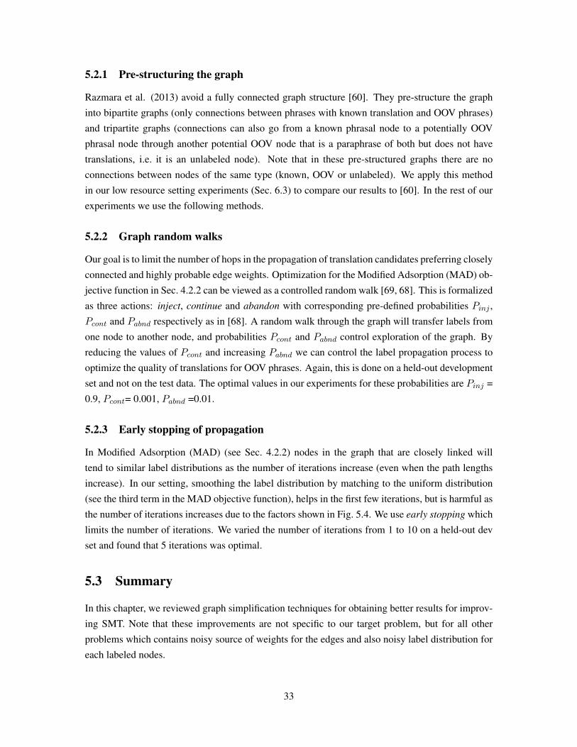
5.2.1 Pre-structuring the graph
Razmara et al. (2013) avoid a fully connected graph structure [60]. They pre-structure the graph
into bipartite graphs (only connections between phrases with known translation and OOV phrases)
and tripartite graphs (connections can also go from a known phrasal node to a potentially OOV
phrasal node through another potential OOV node that is a paraphrase of both but does not have
translations, i.e. it is an unlabeled node). Note that in these pre-structured graphs there are no
connections between nodes of the same type (known, OOV or unlabeled). We apply this method
in our low resource setting experiments (Sec. 6.3) to compare our results to [60]. In the rest of our
experiments we use the following methods.
5.2.2 Graph random walks
Our goal is to limit the number of hops in the propagation of translation candidates preferring closely
connected and highly probable edge weights. Optimization for the Modified Adsorption (MAD) ob-
jective function in Sec. 4.2.2 can be viewed as a controlled random walk [69, 68]. This is formalized
as three actions: inject, continue and abandon with corresponding pre-defined probabilities Pinj ,
Pcont and Pabnd respectively as in [68]. A random walk through the graph will transfer labels from
one node to another node, and probabilities Pcont and Pabnd control exploration of the graph. By
reducing the values of Pcont and increasing Pabnd we can control the label propagation process to
optimize the quality of translations for OOV phrases. Again, this is done on a held-out development
set and not on the test data. The optimal values in our experiments for these probabilities are Pinj =
0.9, Pcont= 0.001, Pabnd =0.01.
5.2.3 Early stopping of propagation
In Modified Adsorption (MAD) (see Sec. 4.2.2) nodes in the graph that are closely linked will
tend to similar label distributions as the number of iterations increase (even when the path lengths
increase). In our setting, smoothing the label distribution by matching to the uniform distribution
(see the third term in the MAD objective function), helps in the first few iterations, but is harmful as
the number of iterations increases due to the factors shown in Fig. 5.4. We use early stopping which
limits the number of iterations. We varied the number of iterations from 1 to 10 on a held-out dev
set and found that 5 iterations was optimal.
5.3 Summary
In this chapter, we reviewed graph simplification techniques for obtaining better results for improv-
ing SMT. Note that these improvements are not specific to our target problem, but for all other
problems which contains noisy source of weights for the edges and also noisy label distribution for
each labeled nodes.
33
Chapter 6
Evaluation
We first show the effect of OOVs on translation quality, then evaluate our approach in three different
SMT settings: low resource SMT, domain shift, and morphologically complex languages. In each
case, we compare results of using paraphrases extracted by Distributional Profile (DP) and PPDB
in an end-to-end SMT system.
Important: no subset of the test data is used in the paraphrase extraction process.
6.1 Experimental Setup
We use CDEC1 [19] as an end-to-end SMT pipeline with its standard features2. fast_align [18]
is used for word alignment, and weights are tuned by minimizing BLEU loss on the dev set using
MIRA [15]. This setup is used for most of our experiments: oracle (Sec. 6.2), domain adaptation
(Sec. 6.4) and morphologically complex languages (Sec. 6.5). But as we wish to fairly compare our
approach with Razmara et al. (2013) [60] on low resource setting, we follow their setup in Sec. 6.3:
Moses [35] as SMT pipeline, GIZA++ [54] for word alignment and MERT [52] for tuning. We add
our own feature as described in Sec. 4.3.
KenLM [25] is used to train a 5-gram language model on English Gigaword (V5: LDC2011T07).
For scalable graph propagation we use the Junto framework3. We use maximum phrase length 10
to make it computationally intractable in propagation and decoding phases.
For French, we apply a simple heuristic to detect named entities: words that are capitalized in
the original dev/test set that do not appear at the beginning of a sentence are named entities. The
reasons to use this simple heuristic is the fact that no accurate named entities recognizer is available
for many resource poor languages. Note that using a more accurate named-entity recognizer and
more removal of named-entities will improve the results even more. Based on eyeballing the results,
this works very well in our data. For Arabic, AQMAR is used to exclude named-entities [48].1http://www.cdec-decoder.org2EgivenFCoherent, SampleCountF, CountEF, MaxLexFgivenE, MaxLexEgivenF, IsSingletonF, IsSingletonEF3Junto : https://github.com/parthatalukdar/junto
34
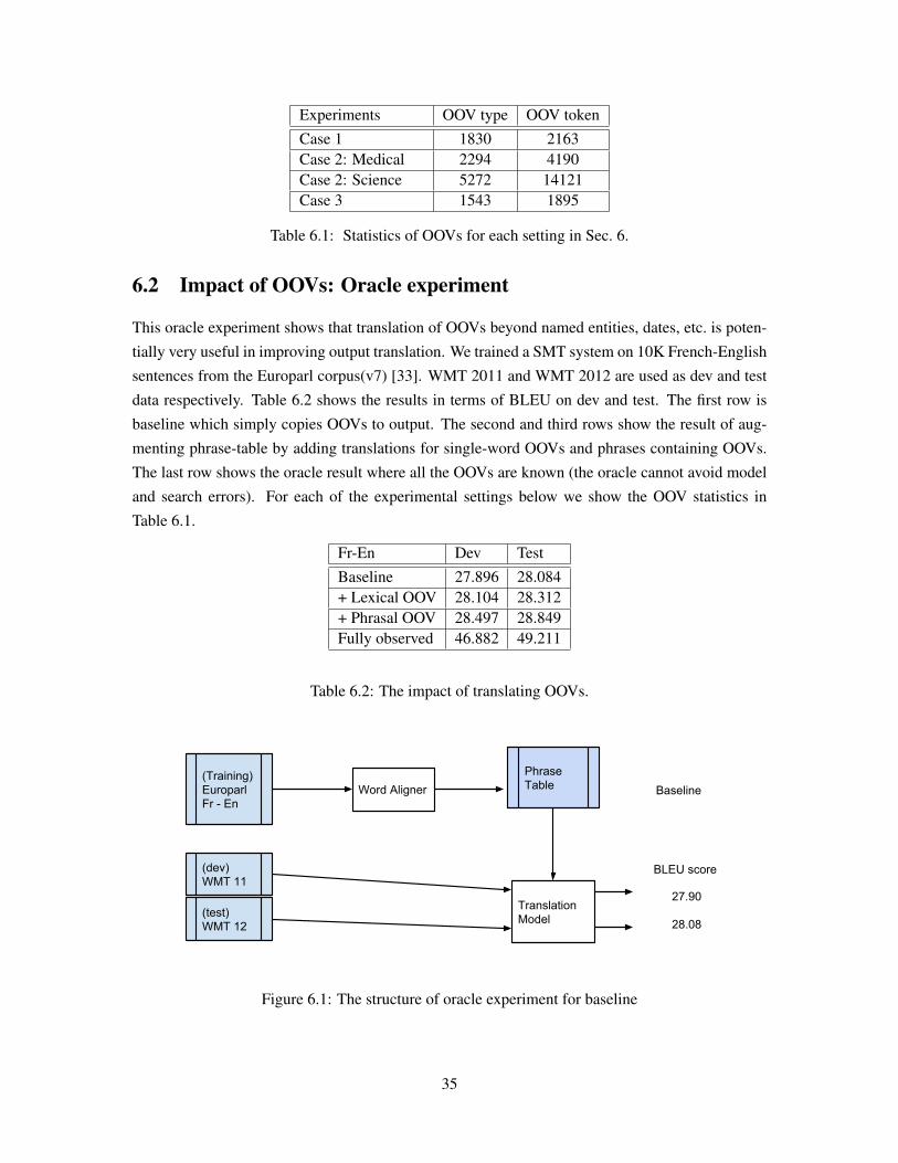
Experiments OOV type OOV tokenCase 1 1830 2163Case 2: Medical 2294 4190Case 2: Science 5272 14121Case 3 1543 1895
Table 6.1: Statistics of OOVs for each setting in Sec. 6.
6.2 Impact of OOVs: Oracle experiment
This oracle experiment shows that translation of OOVs beyond named entities, dates, etc. is poten-
tially very useful in improving output translation. We trained a SMT system on 10K French-English
sentences from the Europarl corpus(v7) [33]. WMT 2011 and WMT 2012 are used as dev and test
data respectively. Table 6.2 shows the results in terms of BLEU on dev and test. The first row is
baseline which simply copies OOVs to output. The second and third rows show the result of aug-
menting phrase-table by adding translations for single-word OOVs and phrases containing OOVs.
The last row shows the oracle result where all the OOVs are known (the oracle cannot avoid model
and search errors). For each of the experimental settings below we show the OOV statistics in
Table 6.1.
Fr-En Dev TestBaseline 27.896 28.084+ Lexical OOV 28.104 28.312+ Phrasal OOV 28.497 28.849Fully observed 46.882 49.211
Table 6.2: The impact of translating OOVs.
Word Aligner(Training)Europarl Fr - En
(dev) WMT 11
(test) WMT 12
Phrase Table
Translation Model
BLEU score
Baseline
27.90
28.08
phrasal OOVs gold translations
Figure 6.1: The structure of oracle experiment for baseline
35
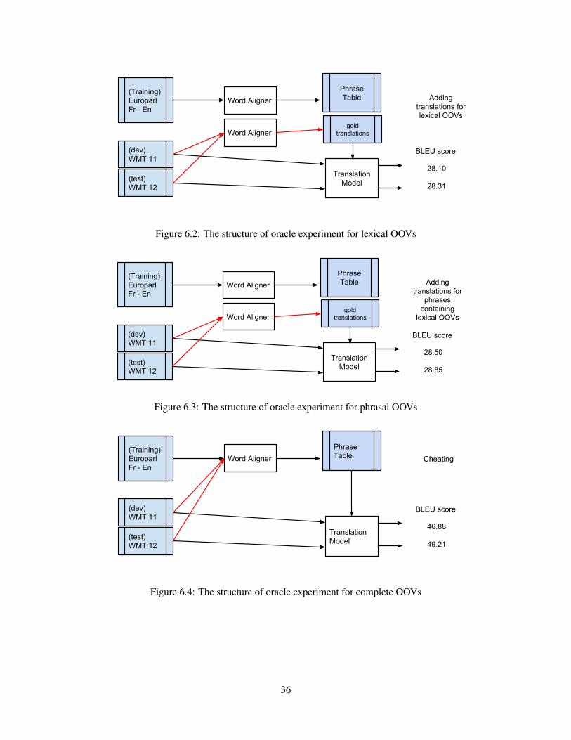
Word Aligner(Training)Europarl Fr - En
(dev) WMT 11
(test) WMT 12
Phrase Table
Translation Model
BLEU score
Adding translations for lexical OOVs
28.10
28.31
gold translationsWord Aligner
Figure 6.2: The structure of oracle experiment for lexical OOVs
Word Aligner(Training)Europarl Fr - En
(dev) WMT 11
(test) WMT 12
Phrase Table
Translation Model
BLEU score
Adding translations for
phrases containing
lexical OOVs
28.50
28.85
gold translationsWord Aligner
Figure 6.3: The structure of oracle experiment for phrasal OOVs
Word Aligner(Training)Europarl Fr - En
(dev) WMT 11
(test) WMT 12
Phrase Table
Translation Model
BLEU score
Cheating
46.88
49.21
phrasal OOVs gold translations
Figure 6.4: The structure of oracle experiment for complete OOVs
36
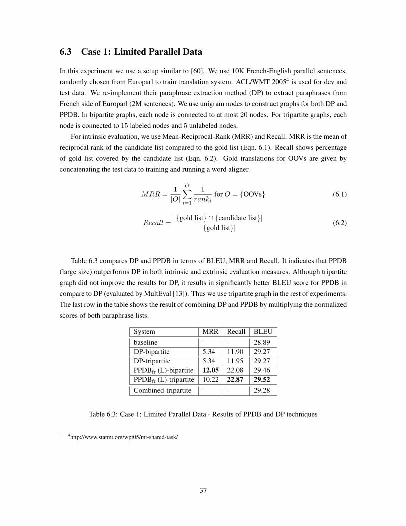
6.3 Case 1: Limited Parallel Data
In this experiment we use a setup similar to [60]. We use 10K French-English parallel sentences,
randomly chosen from Europarl to train translation system. ACL/WMT 20054 is used for dev and
test data. We re-implement their paraphrase extraction method (DP) to extract paraphrases from
French side of Europarl (2M sentences). We use unigram nodes to construct graphs for both DP and
PPDB. In bipartite graphs, each node is connected to at most 20 nodes. For tripartite graphs, each
node is connected to 15 labeled nodes and 5 unlabeled nodes.
For intrinsic evaluation, we use Mean-Reciprocal-Rank (MRR) and Recall. MRR is the mean of
reciprocal rank of the candidate list compared to the gold list (Eqn. 6.1). Recall shows percentage
of gold list covered by the candidate list (Eqn. 6.2). Gold translations for OOVs are given by
concatenating the test data to training and running a word aligner.
MRR = 1|O|
|O|∑i=1
1ranki
for O = {OOVs} (6.1)
Recall = |{gold list} ∩ {candidate list}||{gold list}|
(6.2)
Table 6.3 compares DP and PPDB in terms of BLEU, MRR and Recall. It indicates that PPDB
(large size) outperforms DP in both intrinsic and extrinsic evaluation measures. Although tripartite
graph did not improve the results for DP, it results in significantly better BLEU score for PPDB in
compare to DP (evaluated by MultEval [13]). Thus we use tripartite graph in the rest of experiments.
The last row in the table shows the result of combining DP and PPDB by multiplying the normalized
scores of both paraphrase lists.
System MRR Recall BLEUbaseline - - 28.89DP-bipartite 5.34 11.90 29.27DP-tripartite 5.34 11.95 29.27PPDBfr (L)-bipartite 12.05 22.08 29.46PPDBfr (L)-tripartite 10.22 22.87 29.52Combined-tripartite - - 29.28
Table 6.3: Case 1: Limited Parallel Data - Results of PPDB and DP techniques
4http://www.statmt.org/wpt05/mt-shared-task/
37
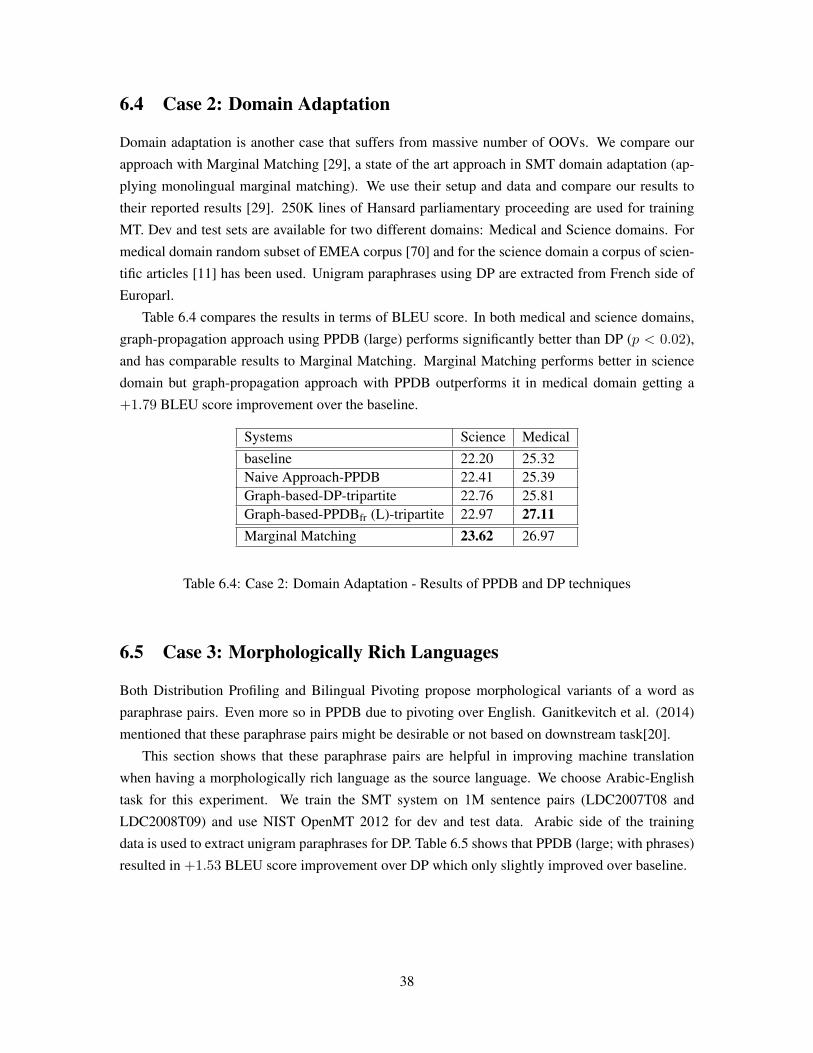
6.4 Case 2: Domain Adaptation
Domain adaptation is another case that suffers from massive number of OOVs. We compare our
approach with Marginal Matching [29], a state of the art approach in SMT domain adaptation (ap-
plying monolingual marginal matching). We use their setup and data and compare our results to
their reported results [29]. 250K lines of Hansard parliamentary proceeding are used for training
MT. Dev and test sets are available for two different domains: Medical and Science domains. For
medical domain random subset of EMEA corpus [70] and for the science domain a corpus of scien-
tific articles [11] has been used. Unigram paraphrases using DP are extracted from French side of
Europarl.
Table 6.4 compares the results in terms of BLEU score. In both medical and science domains,
graph-propagation approach using PPDB (large) performs significantly better than DP (p < 0.02),
and has comparable results to Marginal Matching. Marginal Matching performs better in science
domain but graph-propagation approach with PPDB outperforms it in medical domain getting a
+1.79 BLEU score improvement over the baseline.
Systems Science Medicalbaseline 22.20 25.32Naive Approach-PPDB 22.41 25.39Graph-based-DP-tripartite 22.76 25.81Graph-based-PPDBfr (L)-tripartite 22.97 27.11Marginal Matching 23.62 26.97
Table 6.4: Case 2: Domain Adaptation - Results of PPDB and DP techniques
6.5 Case 3: Morphologically Rich Languages
Both Distribution Profiling and Bilingual Pivoting propose morphological variants of a word as
paraphrase pairs. Even more so in PPDB due to pivoting over English. Ganitkevitch et al. (2014)
mentioned that these paraphrase pairs might be desirable or not based on downstream task[20].
This section shows that these paraphrase pairs are helpful in improving machine translation
when having a morphologically rich language as the source language. We choose Arabic-English
task for this experiment. We train the SMT system on 1M sentence pairs (LDC2007T08 and
LDC2008T09) and use NIST OpenMT 2012 for dev and test data. Arabic side of the training
data is used to extract unigram paraphrases for DP. Table 6.5 shows that PPDB (large; with phrases)
resulted in +1.53 BLEU score improvement over DP which only slightly improved over baseline.
38
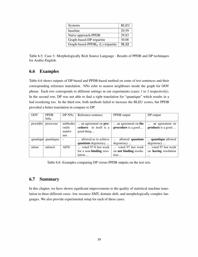
Systems BLEUbaseline 29.59Naive approach-PPDB 29.83Graph-based-DP-tripartite 30.08Graph-based-PPDBfr (L)-tripartite 31.12
Table 6.5: Case 3: Morphologically Rich Source Language - Results of PPDB and DP techniquesfor Arabic-English.
6.6 Examples
Table 6.6 shows outputs of DP-based and PPDB-based method on some of test sentences and their
corresponding reference translation. NNs refer to nearest neighbours inside the graph for OOV
phrase. Each row corresponds to different settings in our experiments (cases 1 to 3 respectively).
In the second row, DP was not able to find a right translation for “quantique” which results in a
bad reordering too. In the third row, both methods failed to increase the BLEU scores, but PPDB
provided a better translation in compare to DP.
OOV PPDBNNs
DP NNs Reference sentence PPDB output DP output
procédés processus méthodesoutilsmatéri-aux
... an agreement on pro-cedures in itself is agood thing ...
... an agreement on theprocedure is a good ...
... an agreement onproducts is a good ...
quantique quantiques - ... allowed us to achievequantum degeneracy ...
... allowed quantumdegeneracy ...
... quantique alloweddegeneracy ...
mlzm mlzmA ADTr ... voted 97-0 last weekfor a non-binding reso-lution ...
... voted 97 last weekon not binding resolu-tion ...
... voted 97 last weekon having resolution...
Table 6.6: Examples comparing DP versus PPDB outputs on the test sets.
6.7 Summary
In this chapter, we have shown significant improvements to the quality of statistical machine trans-
lation in three different cases: low resource SMT, domain shift, and morphologically complex lan-
guages. We also provide experimental setup for each of these cases.
39
Chapter 7
Conclusion and Future work
We presented improvements to Statistical Machine Translation system to alleviate the problem of
OOVs. In the first part of the thesis research, we focused on the task of automatic paraphrase
extraction and explained the two major method distributional profiling and bilingual pivoting. We
compared these two methods and introduced PPDB, a large-scale paraphrase database extracted
using bilingual pivoting but re-scored using monolingual resource.
Next, we highlighted the importance of the graph-based semi-supervised techniques for im-
proving SMT, followed by an analysis of these methods. In the experiments, we showed that
PPDB-based paraphrases pairs are more accurate than DP-based paraphrase, which results in better
improvements for the task of machine translation. We have shown significant improvements to the
quality of statistical machine translation in three different cases: low resource SMT, domain shift,
and morphologically complex languages. In conclusion, PPDB has been successfully used in other
NLP tasks so far, but for the first time we showed that through the use of semi-supervised graph
propagation, a large scale multilingual paraphrase database can be used to improve the quality of
statistical machine translation.
7.1 Future work
In future work, we would like to include translations for infrequent phrases which are not OOVs.
For example, in Figure 7.1 we used a very resource rich SMT trained on millions lines of English-
French parallel sentence. “early bird” is an unseen or infrequent phrase, which result in a wrong
translation.
Furthermore, we would like to explore new propagation methods that can directly use confi-
dence estimates and control propagation based on label sparsity. One of these methods Graph-Based
Transduction with Confidence (TACO) [56] which consider confidence measure for any possible la-
bels. In other words, it consider noisy seed label distributions.
40
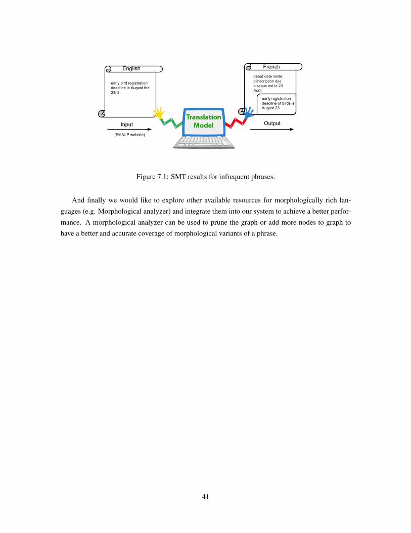
early bird registration deadline is August the 23rd
début date limite d'inscription des oiseaux est le 23 Août.
Input Output
FrenchEnglish
early registration deadline of birds is August 23
(EMNLP website)
Figure 7.1: SMT results for infrequent phrases.
And finally we would like to explore other available resources for morphologically rich lan-
guages (e.g. Morphological analyzer) and integrate them into our system to achieve a better perfor-
mance. A morphological analyzer can be used to prune the graph or add more nodes to graph to
have a better and accurate coverage of morphological variants of a phrase.
41
Bibliography
[1] Andrei Alexandrescu and Katrin Kirchhoff. Graph-based learning for statistical machine trans-lation. In NAACL 2009, 2009.
[2] Satanjeev Banerjee and Alon Lavie. Meteor: An automatic metric for mt evaluation withimproved correlation with human judgments. In Proceedings of the acl workshop on intrinsicand extrinsic evaluation measures for machine translation and/or summarization, volume 29,pages 65–72, 2005.
[3] Colin Bannard and Chris Callison-Burch. Paraphrasing with bilingual parallel corpora. InACL 2005, 2005.
[4] Adam L Berger, Peter F Brown, Stephen A Della Pietra, Vincent J Della Pietra, Andrew SKehler, and Robert L Mercer. Language translation apparatus and method using context-basedtranslation models, April 23 1996. US Patent 5,510,981.
[5] Francis Bond, Eric Nichols, Darren Scott Appling, and Michael Paul. Improving statisticalmachine translation by paraphrasing the training data. In IWSLT 2008, 2008.
[6] Peter F Brown, John Cocke, Stephen A Della Pietra, Vincent J Della Pietra, Fredrick Jelinek,John D Lafferty, Robert L Mercer, and Paul S Roossin. A statistical approach to machinetranslation. Computational linguistics, 16(2):79–85, 1990.
[7] Peter F. Brown, Peter V. deSouza, Robert L. Mercer, Vincent J. Della Pietra, and Jenifer C. Lai.Class-based n-gram models of natural language. Comput. Linguist., 18(4):467–479, December1992.
[8] Peter F Brown, Vincent J Della Pietra, Stephen A Della Pietra, and Robert L Mercer. Themathematics of statistical machine translation: Parameter estimation. Computational linguis-tics, 19(2):263–311, 1993.
[9] Chris Callison-Burch. Syntactic constraints on paraphrases extracted from parallel corpora. InProceedings of the 2008 Conference on Empirical Methods in Natural Language Processing,2008.
[10] Chris Callison-Burch, Philipp Koehn, and Miles Osborne. Improved statistical machine trans-lation using paraphrases. In NAACL 2006, 2006.
[11] Marine Carpuat, H Daumé III, Alexander Fraser, Chris Quirk, Fabienne Braune, Ann Clifton,et al. Domain adaptation in machine translation: Final report. In 2012 Johns Hopkins SummerWorkshop, 2012.
42
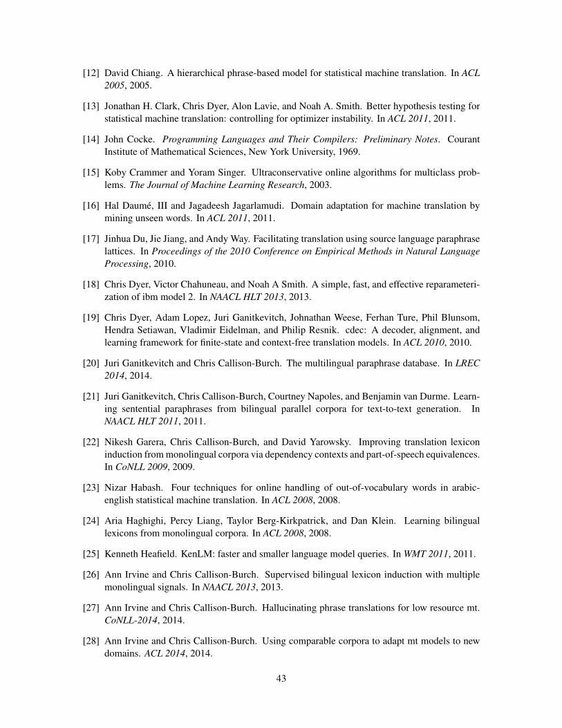
[12] David Chiang. A hierarchical phrase-based model for statistical machine translation. In ACL2005, 2005.
[13] Jonathan H. Clark, Chris Dyer, Alon Lavie, and Noah A. Smith. Better hypothesis testing forstatistical machine translation: controlling for optimizer instability. In ACL 2011, 2011.
[14] John Cocke. Programming Languages and Their Compilers: Preliminary Notes. CourantInstitute of Mathematical Sciences, New York University, 1969.
[15] Koby Crammer and Yoram Singer. Ultraconservative online algorithms for multiclass prob-lems. The Journal of Machine Learning Research, 2003.
[16] Hal Daumé, III and Jagadeesh Jagarlamudi. Domain adaptation for machine translation bymining unseen words. In ACL 2011, 2011.
[17] Jinhua Du, Jie Jiang, and Andy Way. Facilitating translation using source language paraphraselattices. In Proceedings of the 2010 Conference on Empirical Methods in Natural LanguageProcessing, 2010.
[18] Chris Dyer, Victor Chahuneau, and Noah A Smith. A simple, fast, and effective reparameteri-zation of ibm model 2. In NAACL HLT 2013, 2013.
[19] Chris Dyer, Adam Lopez, Juri Ganitkevitch, Johnathan Weese, Ferhan Ture, Phil Blunsom,Hendra Setiawan, Vladimir Eidelman, and Philip Resnik. cdec: A decoder, alignment, andlearning framework for finite-state and context-free translation models. In ACL 2010, 2010.
[20] Juri Ganitkevitch and Chris Callison-Burch. The multilingual paraphrase database. In LREC2014, 2014.
[21] Juri Ganitkevitch, Chris Callison-Burch, Courtney Napoles, and Benjamin van Durme. Learn-ing sentential paraphrases from bilingual parallel corpora for text-to-text generation. InNAACL HLT 2011, 2011.
[22] Nikesh Garera, Chris Callison-Burch, and David Yarowsky. Improving translation lexiconinduction from monolingual corpora via dependency contexts and part-of-speech equivalences.In CoNLL 2009, 2009.
[23] Nizar Habash. Four techniques for online handling of out-of-vocabulary words in arabic-english statistical machine translation. In ACL 2008, 2008.
[24] Aria Haghighi, Percy Liang, Taylor Berg-Kirkpatrick, and Dan Klein. Learning bilinguallexicons from monolingual corpora. In ACL 2008, 2008.
[25] Kenneth Heafield. KenLM: faster and smaller language model queries. In WMT 2011, 2011.
[26] Ann Irvine and Chris Callison-Burch. Supervised bilingual lexicon induction with multiplemonolingual signals. In NAACL 2013, 2013.
[27] Ann Irvine and Chris Callison-Burch. Hallucinating phrase translations for low resource mt.CoNLL-2014, 2014.
[28] Ann Irvine and Chris Callison-Burch. Using comparable corpora to adapt mt models to newdomains. ACL 2014, 2014.
43
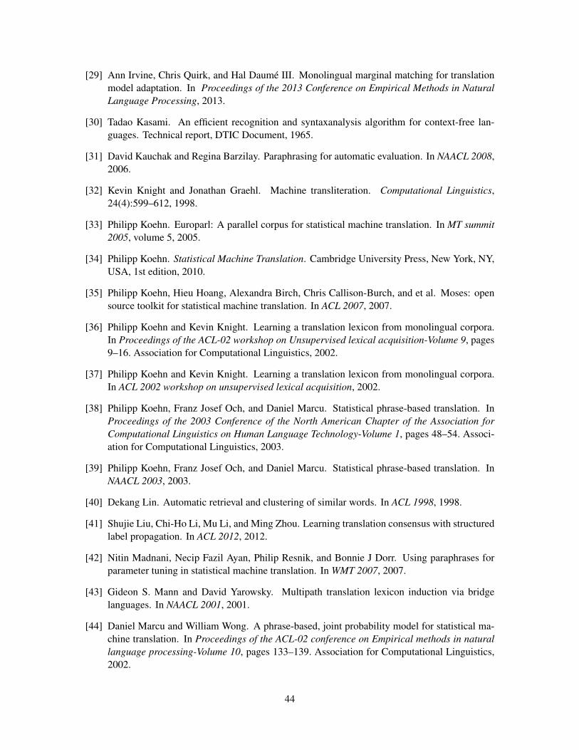
[29] Ann Irvine, Chris Quirk, and Hal Daumé III. Monolingual marginal matching for translationmodel adaptation. In Proceedings of the 2013 Conference on Empirical Methods in NaturalLanguage Processing, 2013.
[30] Tadao Kasami. An efficient recognition and syntaxanalysis algorithm for context-free lan-guages. Technical report, DTIC Document, 1965.
[31] David Kauchak and Regina Barzilay. Paraphrasing for automatic evaluation. In NAACL 2008,2006.
[32] Kevin Knight and Jonathan Graehl. Machine transliteration. Computational Linguistics,24(4):599–612, 1998.
[33] Philipp Koehn. Europarl: A parallel corpus for statistical machine translation. In MT summit2005, volume 5, 2005.
[34] Philipp Koehn. Statistical Machine Translation. Cambridge University Press, New York, NY,USA, 1st edition, 2010.
[35] Philipp Koehn, Hieu Hoang, Alexandra Birch, Chris Callison-Burch, and et al. Moses: opensource toolkit for statistical machine translation. In ACL 2007, 2007.
[36] Philipp Koehn and Kevin Knight. Learning a translation lexicon from monolingual corpora.In Proceedings of the ACL-02 workshop on Unsupervised lexical acquisition-Volume 9, pages9–16. Association for Computational Linguistics, 2002.
[37] Philipp Koehn and Kevin Knight. Learning a translation lexicon from monolingual corpora.In ACL 2002 workshop on unsupervised lexical acquisition, 2002.
[38] Philipp Koehn, Franz Josef Och, and Daniel Marcu. Statistical phrase-based translation. InProceedings of the 2003 Conference of the North American Chapter of the Association forComputational Linguistics on Human Language Technology-Volume 1, pages 48–54. Associ-ation for Computational Linguistics, 2003.
[39] Philipp Koehn, Franz Josef Och, and Daniel Marcu. Statistical phrase-based translation. InNAACL 2003, 2003.
[40] Dekang Lin. Automatic retrieval and clustering of similar words. In ACL 1998, 1998.
[41] Shujie Liu, Chi-Ho Li, Mu Li, and Ming Zhou. Learning translation consensus with structuredlabel propagation. In ACL 2012, 2012.
[42] Nitin Madnani, Necip Fazil Ayan, Philip Resnik, and Bonnie J Dorr. Using paraphrases forparameter tuning in statistical machine translation. In WMT 2007, 2007.
[43] Gideon S. Mann and David Yarowsky. Multipath translation lexicon induction via bridgelanguages. In NAACL 2001, 2001.
[44] Daniel Marcu and William Wong. A phrase-based, joint probability model for statistical ma-chine translation. In Proceedings of the ACL-02 conference on Empirical methods in naturallanguage processing-Volume 10, pages 133–139. Association for Computational Linguistics,2002.
44
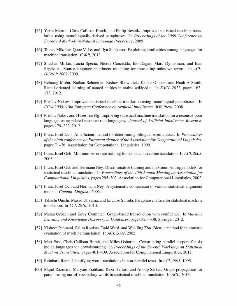
[45] Yuval Marton, Chris Callison-Burch, and Philip Resnik. Improved statistical machine trans-lation using monolingually-derived paraphrases. In Proceedings of the 2009 Conference onEmpirical Methods in Natural Language Processing, 2009.
[46] Tomas Mikolov, Quoc V. Le, and Ilya Sutskever. Exploiting similarities among languages formachine translation. CoRR, 2013.
[47] Shachar Mirkin, Lucia Specia, Nicola Cancedda, Ido Dagan, Marc Dymetman, and IdanSzpektor. Source-language entailment modeling for translating unknown terms. In ACL-IJCNLP 2009, 2009.
[48] Behrang Mohit, Nathan Schneider, Rishav Bhowmick, Kemal Oflazer, and Noah A Smith.Recall-oriented learning of named entities in arabic wikipedia. In EACL 2012, pages 162–173, 2012.
[49] Preslav Nakov. Improved statistical machine translation using monolingual paraphrases. InECAI 2008: 18th European Conference on Artificial Intelligence. IOS Press, 2008.
[50] Preslav Nakov and Hwee Tou Ng. Improving statistical machine translation for a resource-poorlanguage using related resource-rich languages. Journal of Artificial Intelligence Research,pages 179–222, 2012.
[51] Franz Josef Och. An efficient method for determining bilingual word classes. In Proceedingsof the ninth conference on European chapter of the Association for Computational Linguistics,pages 71–76. Association for Computational Linguistics, 1999.
[52] Franz Josef Och. Minimum error rate training for statistical machine translation. In ACL 2003,2003.
[53] Franz Josef Och and Hermann Ney. Discriminative training and maximum entropy models forstatistical machine translation. In Proceedings of the 40th Annual Meeting on Association forComputational Linguistics, pages 295–302. Association for Computational Linguistics, 2002.
[54] Franz Josef Och and Hermann Ney. A systematic comparison of various statistical alignmentmodels. Comput. Linguist., 2003.
[55] Takashi Onishi, Masao Utiyama, and Eiichiro Sumita. Paraphrase lattice for statistical machinetranslation. In ACL 2010, 2010.
[56] Matan Orbach and Koby Crammer. Graph-based transduction with confidence. In MachineLearning and Knowledge Discovery in Databases, pages 323–338. Springer, 2012.
[57] Kishore Papineni, Salim Roukos, Todd Ward, and Wei-Jing Zhu. Bleu: a method for automaticevaluation of machine translation. In ACL 2002, 2002.
[58] Matt Post, Chris Callison-Burch, and Miles Osborne. Constructing parallel corpora for sixindian languages via crowdsourcing. In Proceedings of the Seventh Workshop on StatisticalMachine Translation, pages 401–409. Association for Computational Linguistics, 2012.
[59] Reinhard Rapp. Identifying word translations in non-parallel texts. In ACL 1995, 1995.
[60] Majid Razmara, Maryam Siahbani, Reza Haffari, and Anoop Sarkar. Graph propagation forparaphrasing out-of-vocabulary words in statistical machine translation. In ACL, 2013.
45
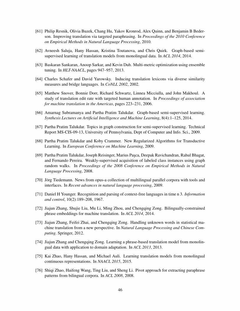
[61] Philip Resnik, Olivia Buzek, Chang Hu, Yakov Kronrod, Alex Quinn, and Benjamin B Beder-son. Improving translation via targeted paraphrasing. In Proceedings of the 2010 Conferenceon Empirical Methods in Natural Language Processing, 2010.
[62] Avneesh Saluja, Hany Hassan, Kristina Toutanova, and Chris Quirk. Graph-based semi-supervised learning of translation models from monolingual data. In ACL 2014, 2014.
[63] Baskaran Sankaran, Anoop Sarkar, and Kevin Duh. Multi-metric optimization using ensembletuning. In HLT-NAACL, pages 947–957, 2013.
[64] Charles Schafer and David Yarowsky. Inducing translation lexicons via diverse similaritymeasures and bridge languages. In CoNLL 2002, 2002.
[65] Matthew Snover, Bonnie Dorr, Richard Schwartz, Linnea Micciulla, and John Makhoul. Astudy of translation edit rate with targeted human annotation. In Proceedings of associationfor machine translation in the Americas, pages 223–231, 2006.
[66] Amarnag Subramanya and Partha Pratim Talukdar. Graph-based semi-supervised learning.Synthesis Lectures on Artificial Intelligence and Machine Learning, 8(4):1–125, 2014.
[67] Partha Pratim Talukdar. Topics in graph construction for semi-supervised learning. TechnicalReport MS-CIS-09-13, University of Pennsylvania, Dept of Computer and Info. Sci., 2009.
[68] Partha Pratim Talukdar and Koby Crammer. New Regularized Algorithms for TransductiveLearning. In European Conference on Machine Learning, 2009.
[69] Partha Pratim Talukdar, Joseph Reisinger, Marius Pasca, Deepak Ravichandran, Rahul Bhagat,and Fernando Pereira. Weakly-supervised acquisition of labeled class instances using graphrandom walks. In Proceedings of the 2008 Conference on Empirical Methods in NaturalLanguage Processing, 2008.
[70] Jörg Tiedemann. News from opus-a collection of multilingual parallel corpora with tools andinterfaces. In Recent advances in natural language processing, 2009.
[71] Daniel H Younger. Recognition and parsing of context-free languages in time n 3. Informationand control, 10(2):189–208, 1967.
[72] Jiajun Zhang, Shujie Liu, Mu Li, Ming Zhou, and Chengqing Zong. Bilingually-constrainedphrase embeddings for machine translation. In ACL 2014, 2014.
[73] Jiajun Zhang, Feifei Zhai, and Chengqing Zong. Handling unknown words in statistical ma-chine translation from a new perspective. In Natural Language Processing and Chinese Com-puting. Springer, 2012.
[74] Jiajun Zhang and Chengqing Zong. Learning a phrase-based translation model from monolin-gual data with application to domain adaptation. In ACL 2013, 2013.
[75] Kai Zhao, Hany Hassan, and Michael Auli. Learning translation models from monolingualcontinuous representations. In NAACL 2015, 2015.
[76] Shiqi Zhao, Haifeng Wang, Ting Liu, and Sheng Li. Pivot approach for extracting paraphrasepatterns from bilingual corpora. In ACL 2008, 2008.
46

[77] Will Y. Zou, Richard Socher, Daniel Cer, and Christopher D. Manning. Bilingual word em-beddings for phrase-based machine translation. In Proceedings of the 2013 Conference onEmpirical Methods in Natural Language Processing, 2013.
47
Recommended