
8 POWER SYSTEM STABILITY
8.1 Elementary Concepts
Maintaining synchronism between the various elements of a power system has become an important task in power system operation as systems expanded with increasing inter connection
of generating stations and load centres. The electromechanical dynamic behaviour of the prime mover-generator-excitation systems, various types of motors and other types of loads with widely varying dynamic characteristics can be analyzed through some what oversimplified methods for understanding the processes involved. There are three modes of behaviour generally identified for the power system under dynamic condition. They are
(a) Steady state stability
(b) Transient stability
(c) Dynamic stability
Stability is the ability of a dynamic system to remain in the same operating state even after a disturbance that occurs in the system.
Stability when used with reference to a power system is that attribute of the system or part of the system, which enables it to develop restoring forces between the elements thereof, equal to or greater than the disturbing force so as to restore a state of equilibrium between the elements.

260 Power System Analysis
A power system is said to be steady state stable for a specific steady state operating condition, if it returns to the same st~ady state operating condition following a disturbance. Such disturbances are generally small in nature.
A stability limit is the maximum power flow possible through some particular point in the system, when the entire system or part of the system to which the stability limit refers is operating with stability.
Larger disturbances may change the operating state significantly, but still into an acceptable steady state. Such a state is called a transient state.
The third aspect of stability viz. Dynamic stability is generally associated with excitation system response and supplementary control signals involving excitation system. This will be dealt with later.
Instability refers to a conditions involving loss of 'synchronism' which in also the same as 'falling out o'fthe step' with respect to the rest of the system.
8.2 Illustration of Steady State Stability Concept
Consider the synchronous generator-motor system shown in Fig. 8.1. The generator and motor have reactances Xg and Xm respectively. They ~re connected through a line of reactance Xe' The various voltages are indicated.
Xe
Fig. 8.1
From the Fig. 8.1
E=E +J·xJ· g m '
Eg -Em 1= .x where X = X + X + X J gem
Power del ivered to motor by the generator is
P = Re [E J*]
Power System Stability 261
E 2 Eg Em = -g- Cos 90° - Cos (90 + 0)
X X
..... (8.1 )
P is a maximum when 0 = 90°
Eg Em P = --=---
max X ..... (8.2)
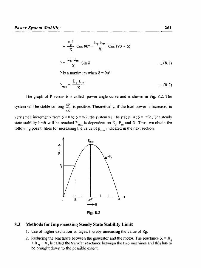
The graph of P versus 0 is called power angle curve and is shown in Fig. 8.2. The
system will be stable so long dP is positive. Theoretically, if the load power is increased in do
very small increments from 0 = 0 to 0 = rr./2, the system will be stable. At 8 = rr./2. The steady
state stability limit will be reached.,p max is dependent on Eg, Em and X. Thus, we obtain the
following possibilities for increasing the value of Pmax indicated in the next section.
Fig. 8.2
8.3 Methods for Improcessing Steady State Stability Limit
1. Use of higher excitation voltages, thereby increasing the value of Eg.
2. Reducing the reactance between the generator and the motor. The reactance X = Xg + Xm + Xe is called the transfer reactance between the two machines and this has to be brought do\\-n to the possible extent.

262 Power System Analysis
8.4 Synchronizing Power Coefficient
Eg Em P = Sin 0
X We have
The quantity
is called Synchronizing power coefficient or stiffness.
For stable operation dP, the synchronizing coefficient must be positive. do
8.5 Transient Stability
..... (8.3)
Steady state stability studies often involve a single machine or the equivalent to a few machines connected to an infinite bus. Undergoing small disturbances. The study includes the behaviour of the machine under small incremental changes in operating conditions about an operating point on small variation in parameters.
When the disturbances are relatively larger or faults occur on the system, the system enters transient state. Transient stability of the system involves non-linear models. Transient
internal voltage E; and transient reactances X~ are used in calculations.
The first swing of the machine (or machines) that occur in a shorter time generally does not include the effect off excitation system and load-frequency control system. The first swing transient stability is a simple study involving a time space not exceeding one second. If the machine remains stable in the first second, it is presumed that it is transient stable for that disturbances. However, where disturbances are larger and require study over a longer period beyond one second, multiswong studies are performed taking into effect the excitation and turbine-generator controls. The inclusion of any control system or supplementary control depends upon the nature of the disturbances and the objective of the study.
8.6 Stability of a Single Machine Connected to Infinite Bus
Consider a synchronous motor connected to an infinite bus. Initially the motor is supplying a mechanical load P rno while operating at a power angle 00, The speed is the synchronous speed ())s' Neglecting losses power in put is equal to the mechanical load supplied. If the load on the motor is suddenly increased to PmI' this sudden load demand will be met by the motor by giving up its stored kinetic energy and the motor, therefore, slows down. The torque angle 0 increases from 00 to 01 when the electrical power supplied equals the mechanical power demand at b as shown in Fig. 8.3. Since, the motor is decelerating, the speed, however, is

Power System Stability 263
less than Ns at b. Hence, the torque 'angle ()' increases further to ()2 where the electrical power Pe is greater than Pml , but N = Ns at point c. At this point c further increase of () is arrested as P e > P ml and N = Ns. The torque angle starts decreasing till °1 is reached at b but due to the fact that till point b is reached Pe is still greater than Pm!' speed is more than Ns. Hence, () decreases further till point a is reacted where N = Ns but Pml > Pe• The cycle of oscillation continues. But, due to the damping in the system that includes friction and losses, the rotor is brought to the new operating point b with speed N = Ns.
In Fig. 8.3 area 'abd' represents deceleration and area bce acceleration. The motor will reach the stable operating point b only if the accelerating energy AI represented by bce equals the decelerating energy A2 represented by area abd.
It
Fig. 8.3 Stability of synchronous motor connected to infinite bus.
8.7 The Swing Equation
The interconnection between electrical and mechanical side of the synchronous machine is provided by the dynamic equation for the acceleration or deceleration ofthe combined-prime mover (turbine) - synchronous machine roter. This is usually called swing equation.
The net torque acting on the rotor of a synchronous machine
where
WR 2
T=--a. g
T = algebraic sum of all torques in Kg-m.
a = Mechanical angular acceleration
WR2 = Moment of Inertia in kg-m2
..... (8.4 )
264 Power System Analysis
Electrical angle ..... (8.5)
Where 11 m is mechanical angle and P is the number of poles
The frequency PN
f= 120
Where N is the rpm.
60f P
rpm 2
(60f) 11e = -- 11m rpm
..... (8.6)
..... (8.7)
The electrical angular position d in radians of the rotor with respect to a synchronously
rotating reference axis is be = 11 e - coot ..... (8.8)
Where Wo = rated synchronous speed in rad./sec
And t = time in seconds (Note: 8 + coat = 11 e)
The angular acceleration taking the second derivative of eqn. (8.8) is given by
From eqn. (8.7) differentiating twice
d 2 11 ( 60 f) d 2 11 _e=l- _m dt 2 rpm dt 2
From eqn. (8.4)
T = WR 2 r rpm) d 2 11 e = WR 2 (rpm ') d 2 8 g ,60f dt 2 g 60f dt 2 ..... (8.9)

Power System Stability
Let the base torque be defined as
torque in per unit
Kinetic energy K.E.
Where
Defining
I WR 2 2
= ---0)0 2 g
') rpm COo = ... 1(--
60
H kinetic energy at rated speed
baseKYA
_ ~ WR 2 (,",1( rpm)2 ___ _ -? g v~ 60 base K Y A
KE atrated speed
265
..... (8.10)
..... (8.11 )
. .... (8.12)
..... (8.13 )
The torque acting on the rotor of a generator includes the mechanical input torque from
the prime mover, torque due to rotational losses [(i.e. friction, windage and core loss)], electrical
output torque and damping torques due to prime mover generator and power system.
The electrical and mechanical torques acting on the rotor of a motor are of opposite sign and are a result of the electrical input and mechanical load. We may neglect the damping and
rotational losses, so that the accelerating torque.
T =T -T a In e
Where Te is the air-gap electrical torque and Tin the mechanical shaft torque.
266 Power System Analysis
..... (8.14)
(i.e.,) d 28 = 7tf (T _ T ) dt2 H In e
..... (8.15)
Torque in per unit is equal to power in per unit if speed deviations are neglected. Then
The eqn. (8.15) and (8.16) are called swing equations.
It may be noted, that, since 8 = S - mot
d8 dS d"t=d"t- mo
Since the rated synchronous speed in rad/sec is 27tf
dS d8 ---+m dt - dt ()
we may put the equation in another way.
1 Kinetic Energy = 2" 1m2 joules
..... (8.16)
The moment of inertia I may be expressed in louie - (Sec)2/(rad)2 since m is in rad/sec. The stored energy of an electrical machine is more usually expressed in mega joules and angles
in degrees. Angular momentum M is thus described by mega joule - sec. per electrical degree
M = l.m
Where m is the synchronous speed of the machine and M is called inertia constant. In practice m is not synchronous speed while the machine swings and hence M is not strictly a constant.
The quantity H defined earlier as inertia constant has the units mega Joules.
stored energy in mega joules H = -----~---.:"---"-----
machine rating in mega voltampers(G)
1 2 1 but stored energy = -1m = - MOl
2 2
..... (8.17)
Power System Stability
In electrical degrees (j) = 360f (= 2nD
1 I GH = - M(360f) = - M2nf = Mnf
2 2
GH M = nf mega joule - sec/elec degree
H In the per unit systems M = nf
So that d20 = nf(p _P)
dt2 H In e
which may be written also as
This is another form of swing equation.
Further
So that
with usual notation.
EV S· s;: p = - lllu e X
8.8 Equal Area Criterion and Swing Equation
267
..... (8.18)
..... (8.19)
..... (8.20)
..... (8.21 )
. .... (8.22)
..... (8.23)
Equal area criterion is applicable to single machine connected to infinite bus. It is not directly applicable to multi machine system. However, the criterion helps in understanding the factors that influence transient stability.
The swing equation connected to infinite bus is given by
H dro --- =p -p =p n f d t 2 mea
..... (8.24)
or ..... (8.25)
268 Power System Analysis
Also ..... (8.26)
Now as t increases to a maximum value 8max where d8 = 0, Multilying eqn (8. I I) on dt
d8 both sides by 2 dt we obtain
2 d28 db = Pa 2 db
dt 2 dt M dt
Integrating both sides
(d8)2 = ~ fp d8 dt M a
db =~~ r<' P d8 dt M 1<>0 a
1t
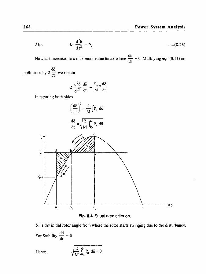
Fig. 8.4 Equal area criterion.
80
is the initial rotor angle from where the rotor starts swinging due to the disturbance.
d8 For Stability dt = °
Hence,

Power System Stability 269
i.e.,
The system is stable, if we could locate a point c on the power angle curve such that areas Al and A2 are equal. Equal area criterion states that whenever, a disturbance occurs, the acclerating and decelerating energies involved in swinging of the rotor of the synchronous
machine must equal so that a stable operating point (such as b) could be located.
But
i.e.,
But
Hence
A I ~ A2 = 0 means that,
P e = P max sin (5
Pm «51 - (50) + Pmax (cos (51 - cos (50) I
P max (cos (51 - cos (52) + P ml «52 - (51) = 0
p ml [(52 - (50] = P max [COS (50 - COS (52)
Pml COS (50 - COS (52 = -P- [(52 - (50]
max
..... (8.27)
The above is a transcendental equation and hence cannot be solved using nonnal algebraic methods.
8.9 Transient Stability Limit
Now consider that the change in Pm is larger than the change shown in Fig. 8.5. This is
illustrated in Fig. 8.5.
In the case AI> A2. That is, we fail to locate an area A2 that is equal to area AI. Then, as stated the machine will loose its stability since the speed cannot be restored to Ns.
Between these two cases of stable and unstable operating cases, there must be a limiting case where A2 is just equal to AI as shown in Fig. 8.6. Any further increase in P ml will cause

270 Power System Analysis
A2 to be less than AI' P ml - P mO in Fig. 8.6 is the maximum load change that the machine can sustain synchronism and is thus the transient stability limit.
180
Fig. 8.5 Unstable system (A1 > A2) .
MW
a pl----f
1t
Fig. 8.6 Transient stability limit.
8.10 Frequency of Oscillations
Consider a small change in the operating angle <>0 due to a transient disturbance by 60. Corresponding to this we can write
0 = 0° + 60
and
where 6Pe is the change in power and POe' the initial power at 0°
(P e + 6P e) = P max sin 0° + P max cos 0°) 60
Power System Stability
Also,
Hence,
Pm = P eO = P max sin 8°
(P m - Peo + ilPe)
= Pmax sin 8° - [P max sin 8° - [P max cos 8°) il8]
= (P max as 8°) il8
P d d~ is the synchronizing coefficient S.
The swing equation is
2H d28° ___ = P = P _ P 0
00 dt 2 a m e
Again,
Hence,
where So is the synchronizing coefficient at Peo.
Therefore,
271
which is a linear second-order differential equation. The solution depends upon the sign of 8°. If 8° is positive, the equation represents simple harmonic motion.
The frequency of the undamped oscillation in
00 =)00 8° m 2 H ..... (8.28)
The frequency f is given by
f = _I)oo80
2n 2 H ..... (8.29)
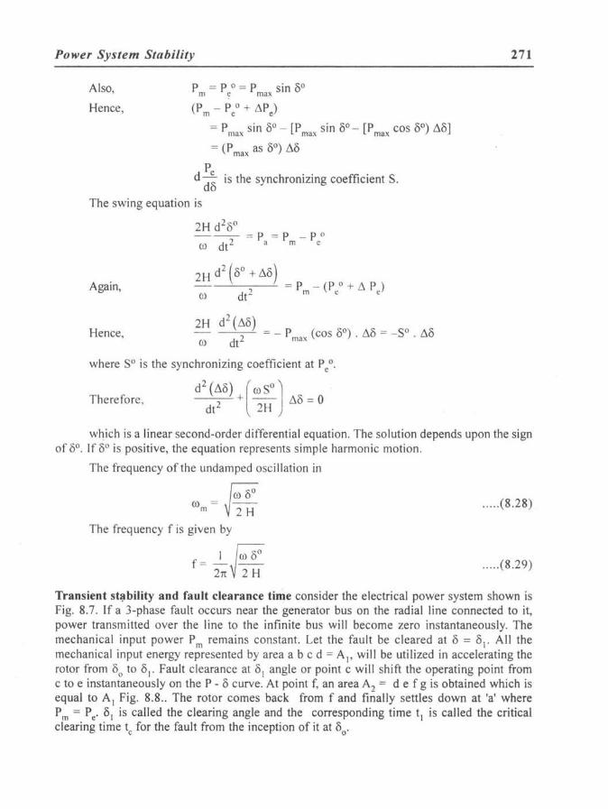
Transient st~bility and fault clearance time consider the electrical power system shown is Fig. 8.7 . If a 3-phase fault occurs near the generator bus on the radial line connected to it, power transmitted over the line to the infinite bus will become zero instantaneously. The mechanical input power Pm remains constant. Let the fault be cleared at 8 = 0\ . All the mechanical input energy represented by area abc d = AI' will be utilized in accelerating the rotor from 8
0 to 8\ . Fault clearance at 8\ angle or point c will shift the operating point from
c to e instantaneously on the P - 8 curve. At point f, an area A2 = d e f g is obtained which is equal to A\ Fig. 8.8 .. The rotor comes back from f and finally settles down at 'a' where Pm = P e' 8\ is called the clearing angle and the corresponding time t\ is called the critical clearing time tc for the fault from the inception of it at 80'

272 Power System Analysis
Line
p Inf. bus
Radial line
Fig. 8.7
8.11 Critical Clearing Time and Critical Clearing Angle
If, in the previous case, the clearing time is increased from tl to tc such that °1 is 0e as shown in Fig. 8.9, Where AI is just equal to A 2, Then, any furter increase in the fault cleaing time tl
Pe
----~------------------~~o 01
Fig. 8.8
beyond te, would not be able to enclosed an area A2 equal to AI' This is shown in Fig. 8.10. Beyond 0e' A2 starts decreasing. Fault clearance cannot be delayed beyond te' This limiting fault clearance angle De is caIled critical clearing angle and the corresponding time to clear the fault is called critical clearing time te'
Pe e
~----------~--~~~8
Fig. 8.9

Power System Stability 273
Fig. 8.10
-From Fig. 8.9-
8max = 1t - 80
Pm = P max sin 00
A2
= (max(Pmaxsina-Pm) deS
= P max (cos <\ - cos 0maJ - Pm (Omax - <\) AI =A2 gives
Pm cos 8 = -- [( 1t - ° ) -° ] + cos (1t - 8 )
C P max o· 0 0
..... (8.30)
During the period of fault the swing equation is given by
dr8 1t f - = - (P - P ). But since P = 0 d t r H me. e

274
During the fault period
dro 1t f -=-P d{ H m
1 dro dt £1tf Integrating both sides --2- = -H Pm dt
dt
do 1tf -=- P t dt H m
and integrating once again
1tf 0=-Pt2 +K
c 2H m
At t = 0; 0 = 00
, Hence K = 00
Hence
Hence the critical cleaning time tc =
Power System Analysis
~.-... (8.3l )
sec. ..... (8.32)
8.12 Fault on a Double-Circit Line
Consider a single generator or generating station sup lying power to a load or an infinite ·bus through a double circuit line as shown in Fig. 8.11.
,
v
Generator ~I------C-~ Infinite bus x~.E
Fig.8.11 Double-circuit line and fault.
EV 1 1 1 The eletrical power transmitted is given by P e = --:--, -- sin 0 where - = - + -
12 Xd + X12 X12 Xl X2
and xd is the transient reactance of the generator. Now, if a fault occurs on line 2 for example,
then the two circuit-brea~ers on either side will open and disconnect the line 2. Since, XI > xI2 (two lines in parallel), the P - 0 curve for one line in operation is given by
EV Pel = sin 0
Xd + xI

Power System Stability 275
. win be below the P - 8 curve P as shwon in Fig. 8.12. The operating point shifts from a to b on p~ curve P e and the rotor ~IJcelerates to poin 0 where 8 = 81, Since the rotor speed is not synchronous, thk rotor decelerates till point d is reched at 8 = 82 so that area AI (= area a b c) is equal to area A2 (= area c d e). The rotor will finally settle down at point c due to damping. At point c
P = P m e l
Fig. 8.12
8.13 Transient Stability When Power is Transmitted During the Fault
Consider the case where during the fault period some load power is supplied to the load or to the infinite bus. If the P-8 curve during the fault is represented by curve 3 in Fig. 8.13 .
p
I I I outpu :during fault
ClUVe 3 d
Fig. 8.13

276 Power System Analysis
Upon the occurrence of fault, the operating point moves from a to b on the during the
fault curve 3. When the fault is cleared at 0 = 0l' the operating point moves from b to c along
the curve Pe3 and then shifts to point e. If area d e f g e could equal area abc d (A2= AI) then
the system wUl be stable.
If the fault clearance is delayed till 81 = Oc as shown in Fig. 8.14 such that area abc d
(A I) is just equal to and e d f (A2) then
r8C (Pmax sino-Pm)do= r,max(pm:x sino-Pm) do ko c
Pel before fault
P.2 after fault
Fig. 8.14 Critical clearing angle-power transmitted during fault.
It is clear from the Fig. 8.14 that 0max = 1t - 00
= 1t - sin-I ~ Pmax2
Integrating
(Pm' 0 + Pmax'COS 0) (: + (pmax 2 COSO-Pm·O) ,tu=O
Pm (Oc - oJ + P max 3 (cos 0c - cos 00 ) + Pm (Omax - 0c)
+ P max2 (cos 0max - cos 0c) = 0
The angles are all in radians.
..... (8.33)

Power System Stability 277
8.14 Fault Clearance and Reclosure in Double-Circuit System
Consider a double circuit system as in section 8.12. If a fault occurs on one of the lines while
supplying a power of P mo; as in the previous case then an area A2 = AI will. be located and the
operating characteristic changes from pre-fault to during the fault. If the faulted line is removed
then power transfer will be again shifted to post-fault characteristic where line I only is in
operation. Subsequently, if the fault is cleared and line 2 is reclosed, the operation once again
shifts back to pre-fault characteristic and normalcy will be restored. For stable operation area
AI (= area abcd) should be equal to areaA2 (= area defghk). The maximum angle the rotor
swings is 53' For stability °2 should be lessthan om' The illustration in Fig. 8.15 assumes fault
clearance and instantaness recJosure.
p
Fig. 8.15 Fault clearance and reclosing .
8.15 Solution to Swing Equation Step-by-Step Method Solution to swing equation gives the change in 5 with time. Uninhibited increase in the value of
5 will cause instability. Hence, it is desired to solve the swing equation to see that the value of
5 starts decreasing after an initial period of increase, so that at some later point in time, the
machine reaches the stable state. Gnerally 8, 5, 3 or 2 cycles are the times suggested for circuit
breaker interruption after the fault occurs. A variety of numerical step-by-step methods are
available for solution to swing equation. The plot of 5 versus t in seconds is called the swing
curve. The step-by-step method suggested here is suitable for hand calculation for a single
machine connected to system.

278 Power System Analysis
Since 8 is changing continuously, both the assumption are not true. When ~t is made very, small, the calculated values become more accurate.
Let the time intervals be ~t
Consider, (n - 2), (n - I) and nth intervals. The accelerating power Pais computed at the end of these intervals and plotted at circles in Fig. 8.16 (a).
(a) Pa(n-2)
Pa(n-2)
Pa (n)
Pa
n-2 n - l n
Assumed (b) Actual
OJ",, - '/,
OJ"n - 312
ffi,
(c)
. -} • _ _ _ _ t./5n
}t./5 - 1 • ___ ___ __ 0
n-2 n - l n
Fig. 8.16 Plotting swing curve.
Note that these are the beginnings for the next intervals viz., (n - I), nand (n + I). Pais kept constant between the mid points of the intervals.
Likewise, wr ' the difference betwen wand W s is kept constant throughout the interval at the value calculated at the mid point. The angular speed therefore is assumed to change between (n - 3/2) and (n - 1/2) ordinates
dO) we know that ~O) = dt' ~t

Power System Stability 279
Note that these are the beginnings for the next intervals viz., (n - I), nand (n + I).
Pais kept constant between the mid points of the intervals.
Likewise, wr' the difference betwen wand Ws is kept constant throughout the interval at
the value calculated at the mid point. The angular ,speed therefore is assumed to change between
(n - 3/2) and (n - 1/2) ordinates
dro we know that ilro = dt' ilt
Hence _ d28 ilt = 180f P ilt
ror(n-l)-ror(n-3/2)- dt 2 ' H a(n-l)' ..... (8.34)
Again change in 8
d8 il8 = dt . ilt
i.e., ..... (8.35)
for (n - I )th inteJl.Yal
and il8n = 8n - 8n _ 1 = ror (n _ 112) • ilt ..... (8.36)
From the two equations (8.16) and (8.15) we obtain
..... (8.37)
Thus, the plot of 8 with time increasing after a transient disturbance has occured or
fault takes place can be plotted as shown in Fig. 8.16 (c).
8.16 Factors Affecting Transient Stability
Transient stability is very much affected by the type of the fault. A three phase dead short
circuit is the most severe fault; the fault severity decreasing with two phase fault and single
line-to ground fault in that order.
If the fault is farther from the generator the severity will be less than in the case of a
fault occurring at the terminals of the generator.
Power transferred during fault also plays a major role. When, part of the power generated
is transferred to the load, the accelerating power is reduced to that extent. This can easily be
understood from the curves of Fig. 8.16.

280 Power System Analysis
Theoretically an increase in the value of inertia constant M reduces the angle through
which the rotor swings farther during a fault. However, this is not a practical proposition
since, increasing M means, increasing the dimensions of the machine, which is uneconomical.
The dimensions of the machine are determined by the output desired from the machine and
stability cannot be the criterion. Also, increasing'M may interfere with speed governing system.
Thus looking at the swing equations
M d 220 = P
a = P _ P = P _ EV Sino
dt m e m Xl2
the possible methods that may improve the transient stability are:
(i) Increase of system voltages, and use of automatic voltage regulators.
(ii) Use of quick response excitation systems
(iii) Compensation for transfer reactance XI2 so that Pe increases and Pm - Pe = PI
reduces.
(iv) Use of high speed circuit breakers which reduce the fault duration time and
hence the acclerating power.
When faults occur, the system voltage drops. Support to the system voltages by automatic
voltage controllers and fast acting excitation systems will improve the power transfer during
the fault and reduce the rotor swing.
Reduction in transfer reactance is possible only when parallel lines are used in place of
single line or by use of bundle conductors. Other theoretical methods such as reducing the
spacing between the conductors-and increasing the size of the conductors dre not practicable
and are uneconomical.
Quick opening of circuit breakers and single pole reclosing is helpful. Since majority of
the faults are line~to-ground faults selective single pole opening and reclosing will ensure transfer
of power during the fault and improve stability.
8.17 Dynamic Stability
Consider a synchronous machine with terminal voltage Vt • The voltage due to excitation acting
along the quadrature axis is Eq and E~ is the voltage along this axis. The direct axis rotor angle
with respect to a synchronously revolving axis is d. If a load change occurs and the field current If is not changed then the various quantities mentioned change with the real power delivered P as shown in Fig. 8.17 (a).

Power System Stability 281
1)
"'I E' q
VI Vt
1)
p
Fig. 8.17 (a)
In case the field current If is changed such that the transient flux linkages along the
q-axis E~ proportional to the field flux linkages is maintained constant the power transfer
could be increased by 30-60% greater than case (a) and the quantities for this case are plotted in Fig. 8.17 (b).
Eq :q I------T---E~ VI 1)
~----------------~p
Fig. 8.17 (b)
If the field current If is changed alongwith P simultaneously so that Vt
is maintained constant, then it is possible to increase power delivery by 50-80% more than case (a). This is shown in Fig. 8.17 (c).
Eq
Eq 1 I::::::::::=----r-- E~ EI
q
Vt
1)
~----------------~p
Fig. 8.17 (c)

282 Power System Analysi~
It can be concluded from the above, that excitation control has a great role to play in power system stability and the speed with which this control is achieved is very important in this context.
E.V Note that Pm ax = X
and increase of E matters in increasing P max'
In Russia and other countries, control signals utilizing the derivatives of output current and terminal voltage deviation have been used for controlling the voltage in addition to propostional control signals. Such a situation is termed 'forced excitation' or 'forced field control'. Not only the first derivatives of L'11 and L'1 Yare used, but also higher derivatives have been used for voltage control on load changes.
There controller have not much control on the first swing stability, but have effect on the operation subsequent swings.
This way of system control for satisfactory operation under changing load conditions using excitation control comes under the purview of dynamci stability.
Power System Stabilizer
An voltage, regulator in the forward path of the exciter-generator system will introduce a damping torque and under heavy load contions'this damping torque may become ndegative. This is a situation where dynamic in stability may occur and casue concern. It is also observed that the several time constants in the forward path of excitation control loop introduce large phase lag at low frequencies just baoe the natural frequency of the excitation system.
To overcome there effects and toi improve the damping, compensating networks are introduced to produce torque in phase with the speed.
Such a network is called "Power System Stabilizer" (PSS).
8.18 Node Elimination Methods
In all stability studies, buses which are excited by internal voltages of the machines only are considered. Hence, load buses are eliminated. As an example consider the system shown in Fig. 8.18.
&J X/l I C\
~,rl>----X-'2-----I~ Infm;to b",
Fig. 8.18
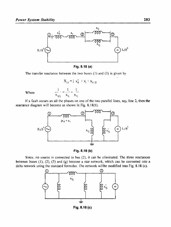
Power System Stability 283
Fig. 8.18 (a)
The transfer reactance between the two buses (I) and (3) is given by
1 1 1 Where --=-+-
X /ll2 XII XIZ
If a fault occurs an all the phases on one of the two parallel lines, say, line 2, then the reactance diagram will become as shown in Fig. 8.18(b).
Fig. 8.18 (b)
Since, no source is connected to bus (2), it can be eliminated. The three reactances between buses (1), (2), (3) and (g) become a star network, which can be converted into a delta network using the standard formulas. The network willbe modified into Fig. 8.18 (c).
<D Q)
Fig. 8.18 (c)

284 Power System Analysis
X:3 is the transfer reactance between buses (I) and (3).
Consider the same example with delta network reproduced as in Fig. 8.18 (d).
Q) t----'
Fig. 8.18 (d)
For a three bus system, the nodal equations are
Since no source is connected to bus (2), it can be eliminated.
Le., 12 has to be mode equal to zero
y 21 V 1 + Y 22 V 2 + Y 23 V 3 = 0
Hence V - Y21 V - Y 23 V 2-- Y 1 Y 3
22 22
This value of V 2 can be substituted in the other two equation of ( ) so that V 2 is eliminated

Power System Stability 185
Worked Examples
E 8. t A 4-pole, 50 Hz, 11 KV turbo generator is rated 75 MW and 0.86 power factor lagging. The machine rotor has a moment of intertia of 9000 Kg-m2. Find the inertia constant in MJ / MVA and M constant or momentum in MJs/elec degree
Solution:
co = 211:f = 100 11: rad/sec
. . 1 2 1 2 Kmetlc energy = 2")eo = 2" x 9000 + (10011:)
= 443.682 x 10⁶ J
= 443.682 MH
75 MYA rating of the machine = 0.86 = 87.2093
MJ 443.682 H = MY A = 87.2093 = 8.08755
GH 87.2093 x 5.08755 M = 180f = 180 x 50
= 0.0492979 MJS/O dc
E 8.2 Two generaton rated at 4-pole, 50 Hz, 50 Mw 0.85 p.f (lag) with moment of inertia 28,000 kg-m1 .ad l-pole, 50Hz, 75 MW 0.82 p.f (lag) with moment of inertia t 5,000 kg_m1 are eoaRected by a transmission line. Find the inertia constant of each machine and tile inertia constant of single equivalent machine connected to infinite bus. Take 100 MVA base.
Solution:
For machine I
1 K.E = 2" x 28,000 x (10011:)2 = 1380.344 x 106 J
50 MVA = 0.85 = 58.8235
1380.344 HI = 58.8235 = 23.46586 MJ!MYA
58.8235 x 23.46586 1380.344 MI =
180 x 50 180x 50
= 0.15337 MJS/degree elect. For the second machine

286 Power System Analysis
1 1 K.E = "2 x 15,000 "2 x (100 n)2 = 739,470,000 J
= 739.470 MJ
75 MVA = 0.82 = 91.4634
739.470 H2 = 91.4634 = 8.0848
91.4634 x 8.0848 M2 = 180 x 50 = 0.082163 MJS/oEIc
M1M2 0.082163xO.15337 M = --'---"--
Ml+M2 0.082163+0.15337
0.0126 0.235533 = 0.0535 MJS/Elec.degree
GH = 180 x 50 x M = 180 x 50 x 0.0535
= 481.5 MJ
on 100 MVA base, inertia constant.
481.5 H = 100 = 4.815 MJIMVA
E 8.3 A four pole synchronous generator rated no MVA 12.5 KV, 50 HZ has an inertia constant of 5.5 MJIMVA
(i) Determine the stored energy in the rotor at synchronous speed.
(ii) When the generator is supplying a load of 75 MW,the input is increased by 10 MW. Determine the rotor acceleration, neglecting losses.
(iii) If the rotor acceleration in (ii) is maintained for 8 cycles, find the change in the torque angle and the rotor speed in rpm at the end of 8 cycles
Solution:
(i) Stored energy = GH = 110 x 5.5 = 605 MJ where G = Machine rating
(ii) P a = The acclerating power = 10 MW
d20 GH d20 10 MW = M dt2 = 180f dt2

Power System Stability 287
=10 180 x 50 dt 2
d28 d28 10 0.0672 dt2 = 10 or dt2 = 0.0672 = 148.81
a = 148.81 elec degrees/sec2
(iii) 8 cyles = 0.16 sec.
Change in 8= !..xI48.8Ix(0.16)2 2
Rotor speed at the end of 8 cycles
__ 120f .(1:) x t __ 120 x 50 P u 4 x 1.904768 x 0.16
= 457.144 r.p.m
E 8.4 Power is supplied by a generator to a motor over a transmission line as shown in Fig. E8.4(a). To the motor bus a capacitor of 0.8 pu reactance per phase is connected through a switch. Determine the steady state power limit with and without the capacitor in the circuit.
Generator~ ~-+I ___ X':':'hn::.::e_=_0_.2.:.P_'U __ ~-+_~ ~Motorv= Ip.u
x l1 =O.lp.u l xl2
=O.lp.u Xd = 0.8p.u T'= E = 1.2p.u
Xc = 0.5p.u
Fig. E.8.4 (a)
Steady state power limit without the capacitor
1.2 x 1 1.2 P = ::=- = 0.6 pu
ma,1 0.8 + 0.1 + 0.2 + 0.8 + 0.1 2.0
With the capacitor in the circuit, the following circuit is obtained.
0.8 0.1 0.2 0.1 0.8
Fig. E.8.4 (b)

288 Power System Analysis
Simplifying
jl.1 j 0.9
E = 1.2 - j 0.8
Fig. E.S.4 (c)
Converting the star to delta network, the transfer reactance between the two nodes X12.
Fig. E.S.4 (d)
(j1.1)(j0.9) + (j0.9)(-jO.8) + (-jO.8 x jl.1) X\2 = -jO.8
-0.99 + 0.72 + 0.88 -0.99 + 1.6 jO.61 ------= =--
- jO.8 - jO.8 0.8
= jO.7625 p.u
1.2x 1 Steady state power limit = 0.7625 = 1.5738 pu
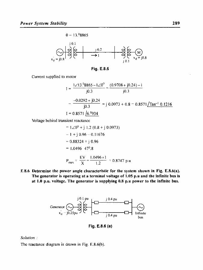
E 8.5 A generator rated 75 MVA is' delivering 0.8 pu power to a motor through a transmission line of reactance j 0.2 p.u. The terminal voltage of the generator is 1.0 p.u and that of the motor is also 1.0p.u. Determine the genera,tor e.m.f behind transient reactance. Find also the maximum power that can be transferred.
Solution:
When the power transferred is 0,8 p.u
1.0 x 1.0 sin a 1 0.8 = (0.1 + 0.2) = 0.3 sin e
- Sin e = 0.8 x 0.3 = 0.24
Power System Stability
j 0.1
,~ ~ ~_+-I __ ~--,=-J O_I·2 __ -+_~ ffi, J 0.1
Fig. E.8.5
Current supplied to motor
lL13.o8865 -lLOo 1=
jO.3
(0.9708 + jO.24) -I
jO.3
-0.0292 + jO.24 jO.3 = j 0.0973 + 0.8 = 0.8571/Tan-1 0.1216
1 = 0.8571 /6.0934
Voltage behind transient reactance
= lLOo + j 1.2 (0.8 + j 0.0973)
= 1 + j 0.96 - 0.11676
= 0.88324 +.i 0.96
= 1.0496 47°.8
EV 1.0496xl Pmax = X = 1.2 = 0.8747 p.u
289
E 8.6 Determine the power angle characteristic for the system shown in Fig. E.8.6(a). The generator is operating at a terminal voltage of 1.05 p.u and the infinite bus is at 1.0 p.u. voltage. The generator is supplying 0.8 p.u power to the infinite bus.
Gen~:: ~.~r--_J_. O_.4_p_u_....,~, j 0.4 pu bus
Fig. E.8.6 (a)
Solution:
The reactance diagram is drawn in Fig. E.8.6(b).

290 Power System Analysis
j 0.4 pu
Fig. E.8.6 (b)
jO.4 The transfer reactance between.V
I and V is = j 0.1 + -2- = j 0.3 p.u
we have Vt V . ~ (1.05)(1.0) . -x Sin u == 0.3 Sin 0 = 0.8
Solving for 0, sin 0 = 0.22857 and 0 = 13°.21
The terminal voltage is 1.05/130.21 '
1.022216 + j 0.24
The current supplied by the generator to the infinite bus
1= 1.022216 + jO.24 - (1 + jO)
jO.3
(0.022216+ jO.24) jO.3 • = 0.8 - j 0.074
= 1.08977/5.°28482 p.u
The transient internal voltage in the generator
EI = (0.8 - j 0.074) j 0.25 + 1.22216 + j 0.24
= j 0.2 + 0.0185 + 1.02216 + j 0.24
= 1 .040 + j 0.44
= 1.1299 /22°.932
The total transfer reactance between El and V
. . jO.4. = J 0.25 + J 0.1 + -2- = J 0.55 p.u
The power angle characteristic is given by
p = E I V sin 0 == (1.1299).(1.0) sin 0 e X jO.55
P e = 2.05436 sin 0

Power System Stability 291
E 8.7 Consider the system in E 8.1 showin in Fig. E.8.7. A three phase fault occurs at point P as shown at the mid pOint on line 2. Determine the power angle characteristic for the system with the fault persisting.
Lme!
Fig. E.8.7
Solution:
The reactance diagram is shown in Fig. E.8.7(a).
i 0.4
Fig. E.S.7 (a)
Infinite bus
The admittance diagram is shown in Fig. E.8.7(b).
- j 2.5
(D...---J
- j 5.0 - j 5.0
Fig. E.8.7 (b)
292 Power System Analysis
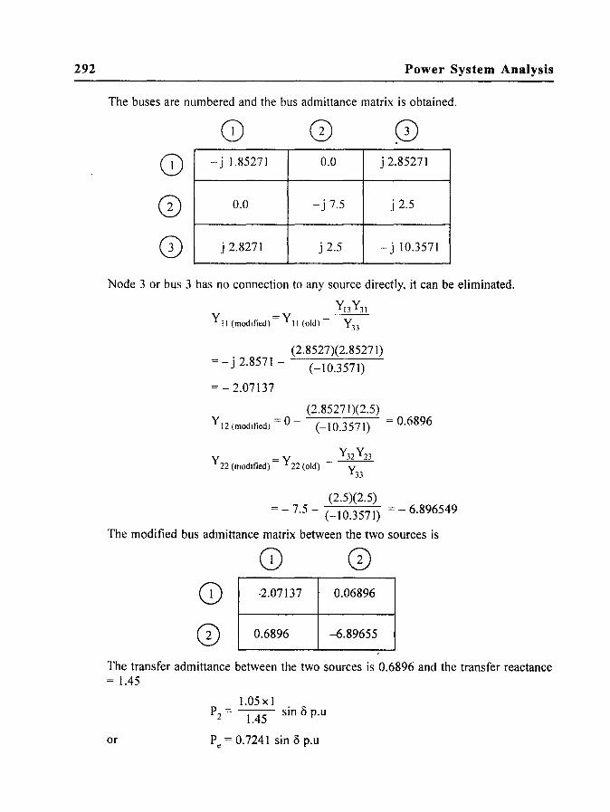
The buses are numbered and the bus admittance matrix is obtained.
(2)
CD
- j 1.85271
0.0
j 2.8271
0.0 j 2.85271
- j 7.5 j 2.5
j 2.5 - j 10.3571
Node 3 or bus 3 has no connection to any source directly, it can be eliminated.
Yl3 Y31 Y II (modIfied) = Y II (old) -~
(2.8527)(2.85271) = - j 2.8571 - (-10.3571)
= - 2.07137
(2.85271)(2.5) Y I2 (modlfied)=0- (-10.3571) =0.6896
_ Y32 Y23 Y22 (modlfied)-Y22 (old) - -Y-
33
(2.5)(2.5) = - 7.5 - (-10.3571) = - 6.896549
The modified bus admittance matrix between the two sources is
CD (2)
CD -2.07137 0.06896
(2) 0.6896 -6.89655
The transfer admittance between the two sources is 0.6896 and the transfer reactance = 1.45
1.05 x 1 P2 = 1.45 sin 8 p.u
or Pe = 0.7241 sin 8 p.u

Power System Stability 293
E 8.8 For the system considered in E.8.6 if the H constant is given by 6 MJ/MVA obtain the swing equation
Solution:
H d20 The swing equation is -f -) = P - Pe = Pa, the acclerating power
7t dt- In
If 0 is in electrical radians
ISOx 50 P _ 6 a - 1500 Pa
E 8.9 In E8.7 jf the 3-phase fault i,s cleared on line 2 by operating the circuit breakers on both sides of the line, determine the post fault power angle characteristic.
Solution: The net transfer reactance between EI and Va with only line 1 operating is
j 0.25 + j 0.1 + j 0.4 = j 0.75 p.u
P = e
(1.05)(1.0)
jO.75 Sin 0 = 1.4 Sin 0
E8.10 Determine the swing equation for the condition in E 8.9 when 0.8 p.u power is delivered.
Given
Solution:
1 M = 1500
ISOf lS0x50 ==
H 6
1 d20
= 1500
1500 dt2' = O.S - 1.4 sin 0 is the swing equation
where 0 in electrical·degrees.
E8.11 Consider example E 8.6 with the swing equation
Pe = 2.05 sin 0
If the machine is operating at 28° and is subjected to a small transient disturbance, determine the frequency of oscillation and also its period.
Given H = 5.5 MJIMVA
P e = 2.05 sin 28° = 0.9624167
Solution:
dPe do = 2.05 cos 28° = 1.7659

294 Power System Analysis
The angular frequency of oscillation = con
CO = )COSO = 21tx50x1.7659
n 2H 2x5.5
= 7.099888 = 8 elec rad/sec.
I 4 f = - x 8 = - = 1.2739 Hz n 21t 1t
1 1 Period of oscillation = T = fll = 1.2739 = T = 0.785 sec
E8.12 The power angle characteristic for a synchronous generator supplying infinite bus is given by
Pe = 1.25 sin 8
The H constant is 5 sec and initially it is delivering a load of 0.5 p.u. Determine the critical angle.
Solution:
Pmo 0.5 -P- = I 25 = 0.4 = Sind 8
0 ; 80 = 23°.578
max .
Cos 80 = 0.9165
80 in radians = 0.4113
280 = 0.8226
1t - 280 = 2.7287
Cos 8e = 1.09148 - 0.9165 = 0.17498
be = 79°.9215
E8.13 Consider the system shown in Fig. E.8.13.
Fig. E.8.13

Power System Stability 295
x~ = 0.25 p.u
lEI = 1.25 p.u and IVI = 1.0 p.lI ; XI = X2 = 0.4 p.u
Initially the system is operating stable while delivering a load of 1.25 p.lI. Determine the stability of the system when one of the lines is switched off due to a fault.
Solution.
When both the lines are working
1.25 x I 1.25 Pe max = 0.25 + 0.2 = 0.45 = 2.778 p.u
When one line is switched off
At point C
pI = 1.25 x I = 1.25 = emax 0.25 + 0.4 0.65 1.923 p.u
Pea = 2.778 Sin 80 = 1.25 p.u
Sin 80 = 0.45
80 = 26°.7437 = 0.4665 radinas
P~ = 1.923 Sin 8 1 = 1.25
Sin 8 1 = 0.65
81 = 40°.5416
== 0.7072 radian

296 Power· System Analysis
0] 07072
A] = area abc = f(P2-P~)dO= fO.25 -1.923sino)do 00 04665
0.7072
= 1.25 I + 1.923 Cos 0
0.4665
= 0.300625 + (-0.255759) = 0.0450
Maximum area available = area c d f g c = A2 max
Om ax 1t-0 7072
A = 2 max f (P:-P,)do= f (1.923Sino-1.25)do 0] 07072
139°.46
= -1.923 Cos 0 I 40°.5416
= 0.7599 - 1.25 x 1.7256
1.25 (2.4328 - 0.7072)
= 0.7599 - 2.157 = -1.3971 »A]
The system is stable
[Note: area A] is below P2 = 1.25 line and
area A2 is above P 2 = 1.25 line; hence the negative sign]
ES.14 Determine the maximum value of the rotor swing in the example ES.13.
Solution:
Maximum value of the rotor swing is given by condition
AI =A2
AI = 0.044866
02
A2 = f(-1.25 + 1.923 Sino}do oj
= (-1.25 O2 + 1.25 x 0.7072) - 1.923 (Cos O2 - 0.76)
i.e., = + 1.923 Cos O2 + 1.25 °2 = 2.34548 - 0.0450
i.e., = 1.923 Cos O2 + 1.25 °2 = 2.30048
By trial and error °2 = 55°.5

Power System Stability 297
E8.15 The M constant for a power system is 3 x 10⁻⁴ S2/elec. degree
The prefault, during the fault and post fault power angle characteristics are given by
P = 2.45 Sin ° el
and
P = 0.8 Sin ° e2
Pe = 2.00 Sin ° respectively 3
choosing a time interval of 0.05 second obtain the swing curve for a sustained fault on
the system. The prefault power transfer is 0.9 p.u.
SolutIOn:
P = 0.9 = 2.45 Sin ° el °
(0.9 )
The initial power angle 0o = Sin-I 2.45
= 21.55°
At t = 0_ just before the occurrence of fault.
P max = 2.45
Sin 0o = Sin 21 °.55 = 0.3673
Pe = P max Sin 0o = 0.3673 x 2.45 = 0.9
Pa = 0
At t = 0+, just after the occurrence of fault
P max = 0.8; Sin °0 = 0.6373 and hence
Pe = 0.3673 x 0.8 = 0.2938
Pa, the acclerating power = 0.9 - Pe
= 0.9 - 0.2938 = 0.606
Hence, the average acclerating powr at t = 0ave
0+0.606
2 = 0.303
I (~t)2 P _ (0.05 x 0.05) _ _ x _ °
M a - 3 X 10⁻⁴ - 8.33 Pa - 8.33 0.303 - 2 .524
~o = 2°.524 and 0° = 21 °.55.
The calculations are tabulated upto t = 0.4 sec.

298 Power S.ystem 1nalysis
Table 8.1
S.No t (sec) Pmax Sin .s P = P = (~t)2 M .s --• a M
(p.u.) P max Sin .s 0.9- p. p. = 8.33 x p.
I. 0- 2.45 0.3673 0.9 0 - - 2155°
0+ 0.8 0.3673 0.2938 0.606 - - 21.55°
°ave 0.3673 - 0.303 2.524 2°.524 24°.075
2. 0.05 0.8 0.4079 0.3263 0.5737 4.7786 7°.3 24°.075
3. 0.10 0.8 0.5207 0.4166 0.4834 4.027 II °.327° 31.3766
4. 0.15 0.8 0.6782 0.5426 0.3574 2.977 14°.304 42°.7036
5. 0.20 0.8 08357 0.6709 0.2290 1.9081 16°.212 570.00
6. 0.25 0.8 0.9574 0.7659 0.1341 1.1170 170.329 73°.2121
7. 0.30 0.8 0.9999 0.7999 0.1000 08330 18°.1623 90.5411
8. 0.35 0.8 0.9472 0.7578 0.1422 1.1847 19°.347 108.70
9 0.40 0.8 0.7875 0.6300 0.2700 2.2500 21°.596 128.047
149°.097
Table of results for E8.1S.
From the table it can be seen that the angle 0 increases continuously indicating instability.
160 E (8.15)
140 \ '" " tb 120 '"
Curve I
0
<.0 100
1 80
60
40
• 20
0.0 0.1 0.2 0.3 0.4 • 0.5 t(sec)~
Power System Stability 299
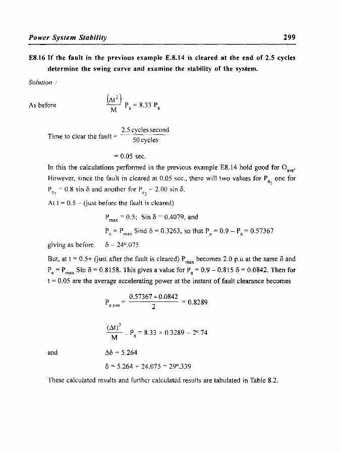
ES. t 6 If the fault in the previous example E.S. t 4 is cleared at the end of 2.5 cycles
determine the swing curve and examine the stability of the system.
Solution:
As before (M2 )
P = 8 33 P M a . a
2.5 cycles second Time to clear the fault = 50 cycles
= 0.05 sec.
In this the calculations performed in the previous example E8. 14 hold good for Dave'
However, since the fault in cleared at 0.05 sec., there will two values for P one for a1
Pe = 0.8 sin 8 and another for P = 2.00 sin 8. 2 e3
At t = 0.5 - Gust before the fault is cleared)
P max = 0.5; Sin 8 = 0.4079, and
Pe = P max Sind 8 = 0.3263, so that Pa = 0.9 - Pe = 0.57367
giving as before 8 = 24°.075
But, at t = 0.5+ Gust after the fault is cleared) P max becomes 2.0 p.u at the same 8 and
Pe = P max Sin 8 = 0.8158. This gives a value for Pa = 0.9 - 0.8158 = 0.0842. Then for
t = 0.05 are the average accelerating power at the instant of fault clearance becomes
and
Pa ave = 0.57367 + 0.0842
2 = 0.8289
(~t)2 M . Pa = 8.33 x 0.3289 = 2°.74
A8 = 5.264
8 = 5.264 + 24.075 = 29°.339
These calculated results and further calculated results are tabulated in Table 8.2.

300 Power System Analysis
Table 8.2
S.No t Pm •• Sin /) P = P = (dt)2 d/) /)
• • M
P max Sin /) 0.9 - p. p. = 8.33 x p.
I. 0- 2.45 0.3673 0.9 0 - - 21.55°
O~ 0.8 03673 0.2938 0.606 - - 21.55°
°ave 0.3673 - 0.303 2.524 2.524 24.075
2. 0.05 0.8 0.4079 0.3263 0.5737 - - --
0.05+ 2.0 0.4079 0.858 0.0842 - - -
O.O\ve 0.4079 - 0.3289 2.740 5.264 29.339
3. 0.10 2.0 0.49 0.98 -0.08 -0.6664 4.5976 33.9J67
4. 0.15 2.0 0.558 1.1165 -0.2165 -1.8038 2.7937 36.730
5. 0.20 2.0 0.598 1.1196 -0.296 -2.4664 0.3273 37.05
6. 0.25 2.0 0.6028 1.2056 -0.3056 -2.545 -2.2182 34°.83
7. 0.39 2.0 0.5711 1.1423 -0.2423 -2.018 -4.2366 30°.5933
Table of results for E8.15.
The fact that the increase of angle 8, started decreasing indicates stability of the system.
ES.17 A synchronous generator represented by a voltage source of 1.1 p.u in series with a transient reactance of jO.1S p.u and an inertia constant H = 4 sec is connected to an infinit~ bus through a transmission line. The line has a series reactance of j0.40 p.u while the infinite bus is represented by a voltage source of 1.0 p.u.
The generator is transmitting an active power of 1.0 p.u when a 3-phase fault occurs at its terminals. Determine the critical clearing time and critical clearing angle. Plot the swing curve for a sustained fault..
Solution:

Power System Stability _
8e = COS-I [(1t - 280}sin 8
0 - COS 8
0]
= COS-I [(ISOo - 2 x 30° )Sin 30° - Cos 30° ]
= cos-I[~-0.S66] = COS-I [l.S07]
= 79°.59 Critical clearing angle = 79°.59
Critical clearing time =
49.59 x 3.14 8 - 8 = 79° 59 -30° = 49 59° = rad
e 0 - - ISO
t = e
= 0.S6507 rad
2 x 4 x 0.S6507
Ix3.14x50 = 0.2099 sec
Calculation for the swing curve
Let
_ (ISOf) 2 [\8n-8n_ l + H [\t Pa(n-I)
[\t = 0.05 sec
8n _ 1 =30°
ISOf ISOx50 --=
H 4 = 2250
H I M = ISOf = 2250 = 4.44 x 10⁻⁴
([\t)2 P = (0.05 x 0.05) P = 5.63 P M a (4,44 x 10⁻⁴ ) a a
Accelerating power before the occurrence of the fault = P a- = 2 Sin 80
- 1.0 = 0
Accelerating power immediately after the occrrence of the fault
Pa+ = 2 Sin 80
- 0 = I p.u
0+1
301
Average acclerating powr = -2- = 0.5 p.u. Change in the angle during 0.05 s~c after
fault occurrence.

302
~81 = 5.63 )( 0.5 = iO.81 81 = 30° + 2°.S1 = 32°.S1
The results are plotted in Fig. ES.17.
Power System Analysis
One-machine system swing curve. Fault cleared at Infs 1400
1200 "1' ....
1000 .... , ............ r············\"" ........ t············:···········
800
600
400
200 ....... : ....... ,!' ....... : ...... .
0.2 0.4 0.6 0.8 1.2 1.4 t, sec
Fig. E.8.17 (a)
One-machine system swing curve. Fault cleared at Infs 90r---.---~---r--~---,----r---r---r---~--,
: : : 80 ....... ; ........... \ ......... ..;. .......... \ ............. ( ........ ! ......... ,. .......... : .......... '" ... .
70 ... . ... , ............ i .......... : ........... 1... ......... j ......... + ......... , ......... .i.. ........ ; ......... . : : . : ; : : :
60 ... : .... ; ......... ; .......... ; ....... (·······t········1·········;····· .. ! ........... ; ........ . 50 ..... . . : ...... ~ ........... ~ .. .
40 ....
300~~~--~--~--~---7----~--~--~--~~ 0.06 0.08 0.1 0.12 0.14 0.16 0.18 0.2
t, sec
Fig. E.8.17 (b)
The system is unstable.

Power Sy!tem Stability 303
E8.18 In example no. E8.17, if the fault is cleared in 100 msec, obtain the swing curve.
Solution:
The swing curve is obtained using MATLAB and plotted in Fig. E.S.IS.
One-machine system swing curve. Fault cleared at 0.1 s 70. .' . .
60' ... ; .... , .\~ .. : ........... . : . ~ :
50 .. : .. : ... : :.. ., ...... .
. ':' .• \" 40
30
~: ..... , ..... , :., ........... \ ... ;'.:" .. :'.: .. " .. .
o . ."i~ -10~~ __ ~~ __ ~~ __ ~~ __ ~ __ ~~
o 0.1 0.2 0.3 0.4 0.5 0.6 0.7 0.8 0.9 1 t, sec
Fig. E8.18 The system is stable.
Problems
PS.I A 2 pole, 50 Hz, II KV synchronous generator with a rating of 120 Mw and 0.S7 lagging power factor has a moment of inertia of 12,000 kg-m2. Calculate the constants HandM.
PS.2 A 4-pole synchronous generator supplies over a short line a load of 60 Mw to a load bus. If the maximum steady stae capacity of the transmission line is 110 Mw, determine the maximum sudden increase in the load that can be tolerated by the system without loosing stability.
PS.3 The prefault power angle chracteristic for a generator infinite bus system is given by Pe = 1.62 Sin 0 I .
and the initial load supplied is I R.U. During the fault power angle characteristic is given by . Pe = 0.9 Sin 0
2 Determine the critical clearing angle and the clearing time.
PS.4 Consider the system operating at 50 Hz.
G 81---'1~_P2_-+_0,7_5P_,u ----111--18 1 X = 0.25 p.ll 0
xd = 0.25p.u I LO H=2.3 sec
If a 3-phase fault occurs across the generator terminals plot the swing curve. Plot also the swing curve, if the fault is cleared in 0.05 sec.

304 Power System Analysis
Questions
8.1 Explain the terms
(a) Steady state stability (b) Transient stabiltiy (c) Dynamic stability
8.2 Discuss the various methods of improving steady state stability.
8.3 Discuss the various methods of improving transient stability.
8.4 Explain the term (i) critical clearing angle and (ii) critical clearing time
8.5 Derive an expression for the critical clearing angle for a power system consisting of a single machine supplying to an infinite bus, for a sudden load increment.
8.6 A double circuit line feeds an infinite bus from a power statio'll. If a fault occurs on one of the lines and the line is switched off, derive an expression for the critical clearing angle.
8.7 Explain the equal area critrion.
8.8 What are the various applications of equal area criterion? Explain.
8.9 State and derive the swing equations
8.10 Discuss the method of solution for swing equation.
Recommended


![Unlocking the Power of LinkedIn Career Pages [Webinar]](https://img.pdfslide.us/doc/110x75/55d5a5d5bb61eb57678b462f/unlocking-the-power-of-linkedin-career-pages-webinar.jpg)