Overhead labour costs in a neo-Kaleckian growth model with
autonomous expenditures
Won Jun Nah Associate Professor, School of Economics and Trade, Kyungpook National University, 80 Daehakro, Bukgu, Daegu, 41566 Korea [email protected] Marc Lavoie* Senior Research Chair, University of Sorbonne Paris Cité (University of Paris 13, CEPN) 99 ave. Jean-Baptiste Clément, 93430 Villetaneuse, France [email protected]
*For this research, Lavoie has benefitted in the past from a grant for the study of income
distribution issues provided by the Institute for New Economic Thinking (INET).
July 2018
Abstract One of the most notable features of income distribution is the widening wage
differential among workers: there is a redistribution in favor of top management at the
detriment of ordinary workers. The paper incorporates this distinction between overhead
managerial labour and direct labour into a neo-Kaleckian growth model with target-return
pricing, where an autonomously growing demand component ultimately determines the
long-run path of an economy. Our aim is to explore the role of overhead labour costs in the
coevolution of income distribution and economic growth. When overhead labour is taken
into account, the share of profits becomes an increasing function of the rate of utilization
of capacity. This implies that empirical research based on the post-Kaleckian specification
of the investment function may fail to isolate the pure profitability effects and is likely to
be biased in finding a profit-led regime.
Our model features convergence to a fully-adjusted position in the long run. This
is achieved by simultaneous path-dependent adjustments, both in the normal rate of
utilization of capacity and in the growth rate of sales expected by firms. We examine the
parametric conditions under which the model achieves a wage-led growth regime, in the
2
restricted sense that both the average rates of accumulation and utilization decrease during
the transitional dynamics arising from an upward adjustment of the normal rate of profit.
Moreover, it is shown that a more equitable wage distribution between the ‘working rich’
and the ‘working poor’ will strengthen the wage-led nature of the economy.
Key words: neo-Kaleckian, growth, overhead labour, autonomous expenditures, target-
return pricing
JEL codes: E11, E37, O41
Overhead labour costs in a neo-Kaleckian growth model with autonomous
expenditures
1. INTRODUCTION
The popular success of the book of Thomas Piketty (2014) has rekindled interest in the
study of income inequality (and possibly wealth inequality) among all strands of economic
thought. One of the key features of post-Keynesian economics is its concern with the
effects of changes in functional income distribution on economic activity as well as the
impact of the evolution of economic activity on income distribution. Over the last twenty
years, an enormous literature has been developed by post-Keynesian authors on the
relationship between the profit share, or the wage share, and economic activity or economic
growth, both from a theoretical angle and through empirical studies (Lavoie and
Stockhammer 2013). What the work of Piketty and his colleagues throughout the world
has however also underlined is the importance of income inequality arising from an
unequal income distribution within wageearners – a feature that had been left relatively
unexplored by post-Keynesian authors.
Thus one of most notable feature of income distribution over the last 40 years is the
widening wage differential among workers: there is a redistribution in favor of top
management at the detriment of ordinary workers. How can this be taken into account
within a macroeconomic model of growth and income distribution which, by tradition, only
distinguished between wages and profits, or at best between wages, net profits and rentier
income? In this paper we propose to subdivide wage-earners into two categories, overhead
labour and direct labour. Overhead labour, or white-collar workers, will be associated with
‘rich’ households, and hence with persons holding managerial positions or what the Bureau
of Labor Statistics (BLS) in the United States calls supervisory workers. By contrast, direct
labour, or blue-collar workers, will be associated with ‘poor’ households, and hence as
persons designated as non-supervisory workers.
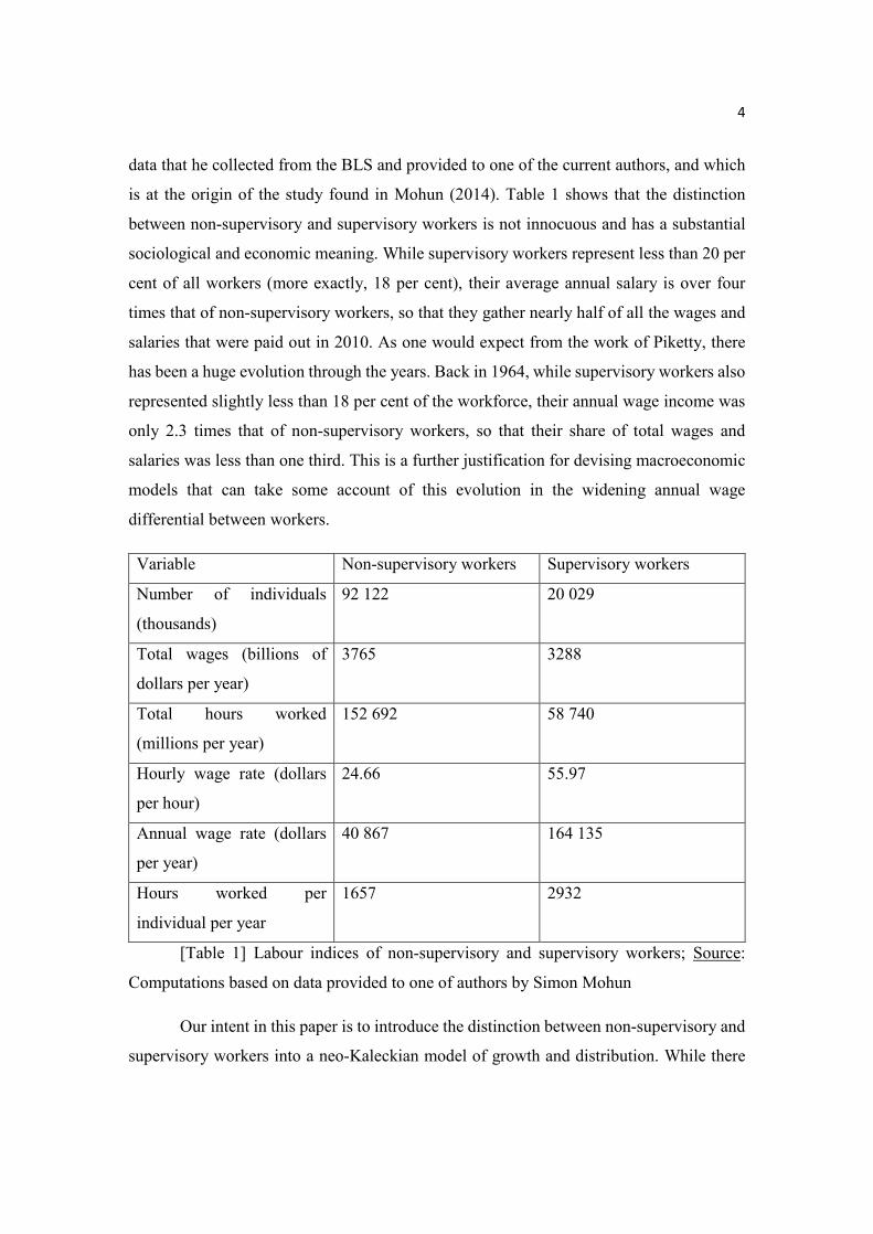
Simon Mohun is one of the few scholars who has taken interest in this distinction
at the empirical level. Table 1 below shows numbers for the year 2010 and is taken from
4
data that he collected from the BLS and provided to one of the current authors, and which
is at the origin of the study found in Mohun (2014). Table 1 shows that the distinction
between non-supervisory and supervisory workers is not innocuous and has a substantial
sociological and economic meaning. While supervisory workers represent less than 20 per
cent of all workers (more exactly, 18 per cent), their average annual salary is over four
times that of non-supervisory workers, so that they gather nearly half of all the wages and
salaries that were paid out in 2010. As one would expect from the work of Piketty, there
has been a huge evolution through the years. Back in 1964, while supervisory workers also
represented slightly less than 18 per cent of the workforce, their annual wage income was
only 2.3 times that of non-supervisory workers, so that their share of total wages and
salaries was less than one third. This is a further justification for devising macroeconomic
models that can take some account of this evolution in the widening annual wage
differential between workers.
Variable Non-supervisory workers Supervisory workers
Number of individuals
(thousands)
92 122 20 029
Total wages (billions of
dollars per year)
3765 3288
Total hours worked
(millions per year)
152 692 58 740
Hourly wage rate (dollars
per hour)
24.66 55.97
Annual wage rate (dollars
per year)
40 867 164 135
Hours worked per
individual per year
1657 2932
[Table 1] Labour indices of non-supervisory and supervisory workers; Source:
Computations based on data provided to one of authors by Simon Mohun
Our intent in this paper is to introduce the distinction between non-supervisory and
supervisory workers into a neo-Kaleckian model of growth and distribution. While there
5
are dozens of such models, only very few of them incorporate this distinction. The first
authors to do so, but in static models, were Asimakopulos (1970) and Harris (1974). In
growth models, the distinction was introduced by Rowthorn (1981), Kurz (1990), Nichols
and Norton (1991), Lavoie (1992, 1995, 1996a, 2009, 2014), and more recently Dutt (2012),
Tavani and Vasudevan (2014), Nikiforos (2017) and Palley (2015, 2017).1
Relative to these previous works, the peculiarity of our paper is that the distinction
between overhead and direct labour is set within a neo-Kaleckian growth model with
autonomously-growing expenditures that do not by themselves create production capacity.
There is now a general recognition that this may be an appropriate way to model basic
stylized facts of modern economies with access to credit. Published papers developing this
new approach, which is related to the so-called Sraffian supermultiplier of Freitas and
Serrano (2015), can be found in Allain (2015; 2018), Lavoie (2016), Nah and Lavoie (2017)
and Hein (2018), with a number of other papers extending this line of research in various
directions, as in Dutt (2015), Lavoie (2017), Nah and Lavoie (2018a; 2018b) and Fazzari
et al. (2018). Indeed, in a sense, this new variant in the way neo-Kaleckian models are
being formalized is closer to the empirical work that has been pursued on the basis of the
post-Kaleckian model of Bhaduri and Marglin (1990). Empirical works assess whether
changes in income distribution have an effect on the level of economic activity while
standard neo-Kaleckian growth models show that such changes affect the growth rate of
economic activity. By contrast the new neo-Kaleckian growth models such as the one
presented here show that changes in income distribution have an effect on the level of
economic activity and not on its growth rate, except as a temporary phenomenon that
occurs during the transition towards the new long-run equilibrium.
The next section presents the key equations of our model, notably how the amount
of direct and overhead labour are determined, and it calculates the algebraic values of the
various shares of income that go to profits, managers and direct labour when firms set
prices on the basis of a target-return pricing formula. We shall see that the profit share and
the share of income going to managers depend on the realized rate of capacity utilization.
1 As far as we know, Rolim (2017) is the only empirical work on wage-led and profit-led demand regimes that splits the wage share into the shares going to supervisory and non-supervisory workers.
6
In the third section we analyze the determinants of the short-run equilibrium, having
previously discussed the shape of the saving and investment functions. In particular we
discuss the conditions under which an increase in the target rate of return or in the wage
rate of managers relative to that of direct workers has a negative impact on the rate of
capacity utilization. In the fourth section, we shall study the long-run equilibrium of the
model. At this stage we introduce two path-dependent adjustments, such that both the
normal rate of capacity utilization and the growth rate of sales expected by firms react to
realized values. We examine the parametric conditions under which the model achieves a
wage-led growth regime, in the restricted sense that both the average rates of accumulation
and of utilization decrease during the transitional dynamics arising from an upward
adjustment of the target rate of return in the pricing equation. We also examine what
happens in the long run when a less equitable wage distribution between the ‘working rich’
and the ‘working poor’ is being imposed to our model economy. In the fifth section, we
report numerical simulation results for the calibrated model as an illustration. The last
section will recap the main innovative features of the model and our main results.
2. THE MODEL ECONOMY
The model economy is a closed economy with no government, where households and
monopolistically competitive firms interact. We borrow the basic assumptions from Lavoie
(2009) for our artificial economy. Firms are owned and managed by a subset of households,
who are the ‘working rich’ in the sense that they comprise shareholders and at the same
time provide managerial, or supervisory, i.e., overhead labour services for the firms. On
the other hand, the rest of households, who are the ‘working poor’, do not save and provide
ordinary, i.e., direct labour services for the firms. The (nominal) wage rate is given by
for direct labour and for overhead labour, where we assume > 1.
The number of direct workers, , varies proportionally to the level of production, , while that of overhead workers, , hinges on productive capacity, . For some
constants and , we have =
and = ⁄ .This implies that direct labour costs are variable and overhead labour
7
costs are fixed with respect to , once the stock of capital, , is given. With ≡ ⁄ ,
we can measure the size of relative to when the economy is operating at full capacity
(when = ). The productivity of direct labour is given by .
National income is divided into profits and wages, and the latter is again divided
into wages to overhead labour and wages to direct labour. Let denote the net share of
profits out of national income, while , where stands for ‘managers’, denotes the share
of national income that goes to overhead labour. Hence, ( + ) amounts to the gross
share of profits. From now on we will refer to as simply the share of profits.
Let us assume that workers involved with direct labour, that is, poor households,
save nothing and consume all their wages. In our model economy, total saving is then made
up of three components: saving from firms, saving from rich households providing
overhead labour, and a negative component, which is dissaving due to autonomous
consumption by rich households. Let us further assume that firms retain a proportion of
their net profits, and that rich households save a constant proportion of both components
of their income, which includes overhead wages and the dividends that they receive from
firms. These dividends are thus a proportion (1 − ) of net profits. We assume that 0 < < 1 and 0 < < 1 . With the real autonomous consumption expenditure, total
saving can then be expressed as: + [ + 1 − ] − [1]
Dividing [1] by , we have a saving function expressed in growth terms, , such that
= + + 1 − −
[2]
where = ⁄ is the rate of utilization of capacity, = ⁄ is the capital-to-capacity
output ratio which is assumed to be constant, and where = ⁄ is the relative magnitude
of autonomous expenditures compared to the volume of capital.
There is quite a bit of empirical evidence that firms use target-return pricing (Lee
8
1998). Under this pricing procedure, the price is set in such a way that a normal rate of
profit will be achieved when the economy is running at the normal rate of utilization of
capacity, i.e., when = .2 Lavoie (2014, p. 333) shows that under these conditions the
price is given by:
= + −
[3]
For [3] to be positive, it must be that >. [4]
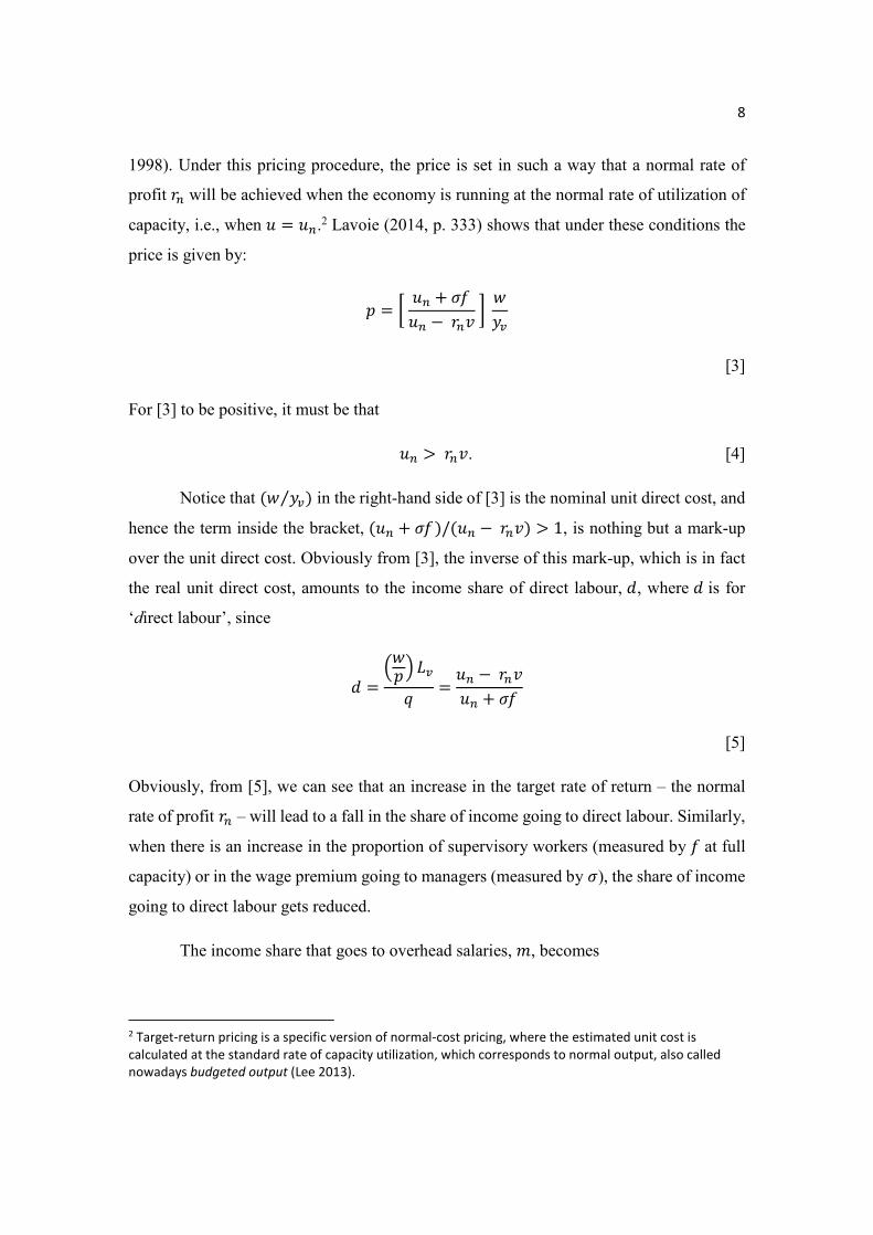
Notice that ( ⁄ ) in the right-hand side of [3] is the nominal unit direct cost, and
hence the term inside the bracket, ( + )/( −) > 1, is nothing but a mark-up
over the unit direct cost. Obviously from [3], the inverse of this mark-up, which is in fact
the real unit direct cost, amounts to the income share of direct labour, , where is for
‘direct labour’, since
= = − +
[5]
Obviously, from [5], we can see that an increase in the target rate of return – the normal
rate of profit – will lead to a fall in the share of income going to direct labour. Similarly,
when there is an increase in the proportion of supervisory workers (measured by at full
capacity) or in the wage premium going to managers (measured by ), the share of income
going to direct labour gets reduced.
The income share that goes to overhead salaries, , becomes
2 Target-return pricing is a specific version of normal-cost pricing, where the estimated unit cost is calculated at the standard rate of capacity utilization, which corresponds to normal output, also called nowadays budgeted output (Lee 2013).
9
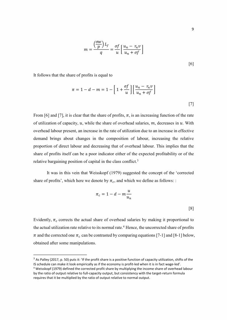
= = − + [6]
It follows that the share of profits is equal to
= 1 − − = 1 − 1 + − + [7]
From [6] and [7], it is clear that the share of profits, , is an increasing function of the rate
of utilization of capacity, , while the share of overhead salaries, , decreases in . With
overhead labour present, an increase in the rate of utilization due to an increase in effective
demand brings about changes in the composition of labour, increasing the relative
proportion of direct labour and decreasing that of overhead labour. This implies that the
share of profits itself can be a poor indicator either of the expected profitability or of the
relative bargaining position of capital in the class conflict.3
It was in this vein that Weisskopf (1979) suggested the concept of the ‘corrected
share of profits’, which here we denote by , and which we define as follows: :
= 1 − −
[8]
Evidently, corrects the actual share of overhead salaries by making it proportional to
the actual utilization rate relative to its normal rate.4 Hence, the uncorrected share of profits and the corrected one can be contrasted by comparing equations [7-1] and [8-1] below,
obtained after some manipulations.
3 As Palley (2017, p. 50) puts it: ‘If the profit share is a positive function of capacity utilization, shifts of the IS schedule can make it look empirically as if the economy is profit-led when it is in fact wage-led’. 4 Weisskopf (1979) defined the corrected profit share by multiplying the income share of overhead labour by the ratio of output relative to full-capacity output, but consistency with the target-return formula requires that it be multiplied by the ratio of output relative to normal output.
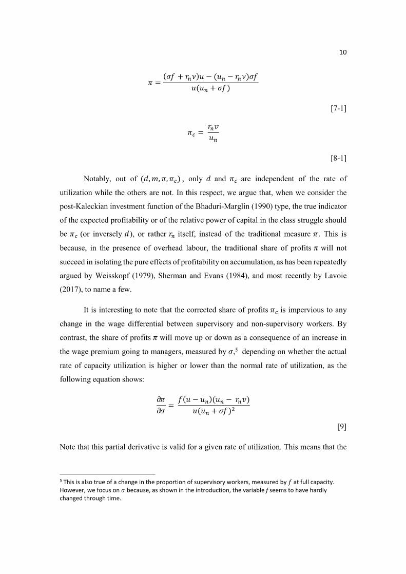
10 = ( + ) − ( − )( + )
[7-1]
=
[8-1]
Notably, out of (,, , ) , only and are independent of the rate of
utilization while the others are not. In this respect, we argue that, when we consider the
post-Kaleckian investment function of the Bhaduri-Marglin (1990) type, the true indicator
of the expected profitability or of the relative power of capital in the class struggle should
be (or inversely ), or rather itself, instead of the traditional measure . This is
because, in the presence of overhead labour, the traditional share of profits will not
succeed in isolating the pure effects of profitability on accumulation, as has been repeatedly
argued by Weisskopf (1979), Sherman and Evans (1984), and most recently by Lavoie
(2017), to name a few.
It is interesting to note that the corrected share of profits is impervious to any
change in the wage differential between supervisory and non-supervisory workers. By
contrast, the share of profits will move up or down as a consequence of an increase in
the wage premium going to managers, measured by ,5 depending on whether the actual
rate of capacity utilization is higher or lower than the normal rate of utilization, as the
following equation shows: = ( − )( −)( + )
[9]
Note that this partial derivative is valid for a given rate of utilization. This means that the
5 This is also true of a change in the proportion of supervisory workers, measured by at full capacity. However, we focus on because, as shown in the introduction, the variable f seems to have hardly changed through time.
11
profit-share curve seen from the supply side [7-1], drawn in (, ) space, shifts down if < and shifts up if > as increases. This is illustrated in [Figure 1].
[Figure 1] around here
We may now deal with the last elements of the model. The saving function can be
reformulated with an explicit consideration of our target-return pricing formula as can be
found in Appendix 1. In this paper, we assume that the investment function takes the
standard form of those neo-Kaleckian models that are concerned with a possible
convergence towards the normal rate of capacity utilization. = + ( − ) [10] is the rate of accumulation of capital, i.e., investment divided by . The first term on
the right-hand side, , represents the secular expected growth rate of sales. The coefficient captures the sensitivity of induced investment to changes in effective demand, i.e., to
changes in the rate of capacity utilization.
3. EQUILIBRIUM IN THE SHORT RUN
For analytical tractability, we introduce a distinction between the short and the long run
into our model economy. We define the short run as the time period during which the
capital stock, , does not change, thus implying that there is no expansion of production
capacity as of yet. It is also assumed that over the short run there is no change in the normal
rate of capacity utilization, , the expectation of the firms about future sales growth, ,
and the autonomous consumption by the working rich, . All these variables will be
allowed to adjust in the long run.
The short-run equilibrium is achieved by adjustments in the rate of utilization of
capacity so as to equate to (so that saving equals investment, or alternatively, so that
aggregate supply equates aggregate demand). The equilibrium rate of utilization of
capacity will be denoted by ∗, as determined in Appendix 1. For the short-run equilibrium
to be stable, the following Keynesian stability condition must be met.
12 (1 − ) + ( + ) − ( + ) ≡ > 0 [11]
We can also obtain the short-run equilibrium values of the share of profits, ∗, the rate of
profit, ∗, and the rate of accumulation, ∗, as found in Appendix 1 .
A simple comparative statics exercise shows that both the short-run equilibrium
values of the rate of capacity utilization and of the rate of accumulation are lower when
there is a higher normal rate of profit . This reveals the wage-led nature of demand and
accumulation of the present model in the short run. ∗ = − (1 − ) + ∗(1 − ) + < 0
[12] ∗ = ∗ < 0
[13]
Furthermore, we can evaluate the short-run effects of widening the gap between
the wage rate obtained by overhead labour and the wage rate of direct labour. We have ∗ = ( − )(1 − ) − ∗(1 − ) + ( + ) . [14]
Three cases need to be considered:
(a) ∗ ⁄ > 0 and ∗ ⁄ > 0, if
∗ < (1 − )(1 − ) + , [14-1]
(b) ∗ ⁄ < 0 and ∗ ⁄ < 0, if
13 ∗ > (1 − )(1 − ) + ,
[14-2]
And finally, (c) ∗ ⁄ = 0 and ∗ ⁄ = 0, if
∗ = (1 − )(1 − ) + . [14-3]
A permanent increase in has a twofold effect. Obviously, it directly increases
overhead expenses incurred by firms. This reallocates income from the firms to the
working rich. With income going to firms, only the ratio (1 − )(1 − ) gets to be spent
on consumption by rich households; with income going directly to the households of the
working rich, the ratio (1 − ) gets spent. The former is strictly less than the latter.
Moreover, when the value of is higher, the difference between the former and the latter
gets bigger. Thus, an increase in may lead to an increase in consumption and in the rate
of utilization as in the (a) case, and this positive redistribution effect is amplified with a
bigger . We can see that, the higher is , the more likely is the (a) case, since the term
inside the squared bracket on the far right of (a) increases in . Notice that ∗ is more
likely to be smaller once the term inside the bracket is big enough, and vice versa. (1 − )(1 − ) + > 0. [15-1]
However, this is not the whole story. As is evident from [5], an increase in lowers
the income share that goes to the households of the working poor, whose propensity to
consume is assumed to be unitary. This is because of the target-return pricing strategy: as
equation [3] shows, an increase in overhead costs will lead to an increase in the mark-up
over direct unit labour costs and hence to a fall in the real wage of direct labour. A widening
gap in wage rates shifts income away from the poor to the rich. Due to the difference in
14
their respective propensities to save, this change yields a shrinking effect on the economy
as in the (b) case. This is to be expected because if rich households receive higher wages
but save most of it, the potential positive effect of this change will be that much smaller.
Also, it is apparent that, as gets smaller, the difference in the propensities to consume
of the poor and the rich diminishes, and hence the negative effect caused by the
redistribution towards the rich is dampened. This makes the (b) case less likely. It is
consistent with the fact that the term in the squared bracket on the far right of (b) decreases
in . (1 − )(1 − ) + < 0. [15-2]
These two effects are in conflict with each other. The former positive effect is due
to the redistribution towards the working rich away from the retained earnings of the firms,
and the latter negative effect is due to the redistribution towards the working rich away
from the working poor. Unless the former dominates the latter, the less equitable structure
of wages resulting from an increase in turns out to reduce effective demand in the short
run, as in the (b) case. From the discussions above, we can conclude that the (b) case is
more likely to occur than the (a) case when the marginal propensity to save of the working
rich, which is , is high and when the retention ratio of firms, which is , is low. We can
also conclude from [14-1] that in the neighbourhood of the normal rate of capacity
utilization , the effect on economic activity of an increase in wage dispersion will be
negative.
Coming now to the effects on the profit share as a consequence of an increase in
the wage premium obtained by overhead labour, i.e., of an increase in wage dispersion, we
plug [6] into the saving function [2], thus obtaining a saving function with only the profit
share and the rate of utilization as endogenous variables, and then equate this saving
function to the investment function [10] to get the profit share as a function of the rate of
utilization:
15 = 1 + (1 − ) − − + + ( − + ) + (1 − )
[7-2]
Equation [7-2] is the profit share seen from the demand side and can be contrasted with [7-
1], which is seen from the opposite cost side. Evaluating the partial derivative with respect
to , while holding the rate of utilization constant in [7-2], we have: = − ( − ) + 1 − ( + ) < 0
[16]
This implies that the profit-share curve seen from the demand side [7-2], drawn in (, ) space, shifts down in a parallel fashion when increases, as is illustrated in either [Figure
2A] or [Figure 2B], depending on whether the term ( − + ) in [7-2] is positive or
negative.
[Figure 2A] around here
[Figure 2B] around here
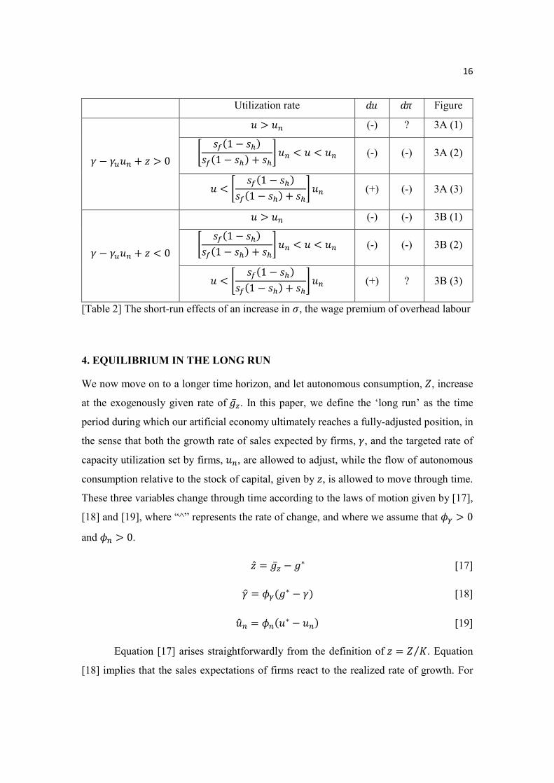
[Table 2] summarizes the effects of an increase in (the wage premium of
overhead labour) on the rate of utilization and on the share of profits when the combined
effects on the demand and supply sides are taken into consideration. With regards to the
impact of an increase in the wage differential on the short-run equilibrium share of profit,
an analytical discussion is provided in Appendix 2. As to the impact of this increase on the
rate of capacity utilization, the possible cases were explained above with the help of
equations [14]. The detailed graphical illustrations corresponding to the various cases of
[Table 2] can be found in [Figure 3A] and [Figure 3B].
[Figure 3A] around here
[Figure 3B] around here
16
Utilization rate Figure
− + > 0
> (-) ? 3A (1) (1 − )(1 − ) + < < (-) (-) 3A (2)
< (1 − )(1 − ) + (+) (-) 3A (3)
− + < 0
> (-) (-) 3B (1) (1 − )(1 − ) + < < (-) (-) 3B (2)
< (1 − )(1 − ) + (+) ? 3B (3)
[Table 2] The short-run effects of an increase in , the wage premium of overhead labour
4. EQUILIBRIUM IN THE LONG RUN
We now move on to a longer time horizon, and let autonomous consumption, , increase
at the exogenously given rate of . In this paper, we define the ‘long run’ as the time
period during which our artificial economy ultimately reaches a fully-adjusted position, in
the sense that both the growth rate of sales expected by firms, , and the targeted rate of
capacity utilization set by firms, , are allowed to adjust, while the flow of autonomous
consumption relative to the stock of capital, given by , is allowed to move through time.
These three variables change through time according to the laws of motion given by [17],
[18] and [19], where “^” represents the rate of change, and where we assume that > 0
and > 0. = − ∗ [17] = (∗ − ) [18] = (∗ − ) [19]
Equation [17] arises straightforwardly from the definition of = ⁄ . Equation
[18] implies that the sales expectations of firms react to the realized rate of growth. For
17
instance, when the actual growth rate of the economy turns out to be unexpectedly high,
the expected growth rate of sales will be modified upwards accordingly. This reaction
function is often referred to as the Harrodian instability mechanism. Equation [19] provides
a long-run endogenous adjustment in the normal rate of capacity utilization. The argument
is that if the realized rates of utilization exceed persistently the rate construed as being
normal, it seems quite possible that firms would change their view about what the normal
rate of utilization ought to be, making it higher, both for their investment and pricing
decisions. Symmetrically, if the actual rate of utilization is systematically below the normal
rate, the convention about what the normal rate ought to be may be given a lower value.
A number of authors in the past have provided different arguments to the effect
that the normal rate of capacity utilization is likely to be influenced by the values being
taken by the actual rate of utilization. The argument was first made by Amadeo (1986) and
Ciccone (1986), and was picked up by Hein et al. (2012) and by Lavoie (1995, 1996b,
2010, 2014) in a number of papers, on the grounds that the normal rate is a convention
adopted by the accountants of the firms that ought to change with past trends. More recently,
more sophisticated arguments have been provided by Dutt (1997), Nikiforos (2016) and
Tavani and Petach (2018), which have been endorsed by Dávila-Fernández et al. (2017).
Thus, the introduction of equation [19] in a neo-Kaleckian growth model is not something
new. Combining equations [18] and [19] in such a model is not new either: it was vaguely
suggested as a possibility in Lavoie (1992: 330) and formalized in Lavoie (1995, 1996b),
in Cassetti (2006) and in Hein et al. (2012).6 The novel feature of the present study is that
we introduce for the first time the combined adjustment mechanisms given by equations
[18] and [19] into the recent Kaleckian literature incorporating autonomous non-capacity
creating expenditures.
As a consequence of the introduction of [19], which makes endogenous the normal
6 The empirical support for this combination has been provided by Lavoie, Rodriguez, and Seccareccia (2004), where they claimed the relevance of the Kaleckian investment equation with hysteresis. Further empirical support can be found in Schoder (2012), Nikiforos (2016) and Setterfield (2017). In addition, Fiebiger (2018b) shows that there is a tight visual relationship between the HP-filtered data representing industry-level rates of utilization and the growth rate of industry value added, thus suggesting some degree of endogeneity in the normal rate of utilization.
18
rate of capacity utilization, the long-run position of the model is not an exogenously given
solution anymore, stuck at a fixed target rate of capacity utilization.
From [17] and [18], the long-run equilibrium solutions are given by: ∗∗ = [20] ∗∗ = [21]
However, there is a caveat. Equations [18] and [19] are not orthogonal, since we
have from [10]:
= . [22]
Let us define an initial point for (, ) to be (, ) . Then the long-run
equilibrium rate of utilization, ∗∗ = ∗∗, can be obtained from [22]:
∗∗ = ∗∗ = 1 + ( − ) [23]
This clearly shows that the final position of the system in its long-run is affected by
its initial condition. In this respect, our long-run equilibrium becomes a path-dependent
equilibrium.
The long-run values of other variables can be determined. Straightforwardly from
[7-1], the long-run share of profits, ∗∗, is equal to
∗∗ = ∗∗ [7-3]
As to the long-run income shares of direct wages, ∗∗, and overhead salaries, ∗∗, they are:
19 ∗∗ = ∗∗ − ∗∗ +
[5-1]
∗∗ = ∗∗ ∗∗ − ∗∗ + [6-1]
Then from [2], we have
∗∗ = (1 − ) + + ∗∗ − ∗∗ + −
[24]
It is shown in Appendix 3 that, essentially, in this model of autonomously growing
non-capacity creating expenditures with overhead labour costs, just as in the standard
model without such costs, the presence of the short-run Keynesian stability condition,
which is > 0 , also guarantees dynamic stability towards a long-run fully-adjusted
position, provided there exists a Harrodian adjustment mechanism tied to the investment
function and provided this Harrodian instability mechanism is sufficiently weak so that it
gets tamed by the growth of autonomous expenditures.
We have seen that should be small enough to meet the stability requirement.
However, as is clear from [18], also governs the adjustment speed of . The smaller is
the value of , the more the system is likely to be stable, but also the slower will be its
process of convergence. We believe this possible trade-off between the probability and the
speed of long-run convergence needs to be carefully handled.
Finally, we evaluate some of the important partial derivatives of ∗∗. ∗∗ = (1 − ) + ∗∗∗∗ + > 0
[25]
20 ∗∗ = ∗∗∗∗(∗∗ + ) > 0
[26]
Recall that the numerator of grows at a constant rate. Hence, [25] implies that
when there is an upward adjustment to the target rate of return set by firms, on average the
stock of capital grows more slowly than do autonomous expenditures (which grow at the
rate ) during the whole traverse between the old and the new long-run equilibrium.
Considering the transition dynamics after the change, we can say that the average rate of
accumulation has gone down. This is indicative of the wage-led nature of growth in the
long run, in the restricted sense that the rate of capital accumulation on average gets
reduced during the traverse, until it reaches a new long-run position after an increase in the
normal rate of profit. This means that the level of output will be lower than otherwise it
would have been if firms had not decided to raise the target rate of return. What we have
is a level effect, similar to those effects identified in empirical work trying to ascertain the
demand regime of an economy.
Likewise, for the same reasons, [26] implies that a widening gap in the wage
obtained by overhead workers relative to that attained by direct workers slows down the
accumulation of capital during the traverse to the new long-run solution. During the
transition period from the initial to the final state, the average rate of accumulation goes
down after an increase in the wage differential between supervisory and non-supervisory
workers. This can be interpreted as supporting the prospect for the so-called ‘income (or
wage) equality-led growth’ and/or ‘solidarity wage policy’.
Last but not least, the wage-led nature of growth in the present model economy,
which is evident from [25], can be shown to be more prominent when wage distribution is
more equitable, and hence when the relative wage gap is smaller. This can be demonstrated
by [27] below. ∗∗ < 0
[27]
21
In words, an economy where wage distribution is highly unequal, all else equal,
will turn out to be less strongly wage-led in the long run. The positive association that our
paper reveals between the wage-led feature of growth and a more equal wage distribution
is in line with the recent claims of Carvalho and Rezai (2016) and Palley (2017).
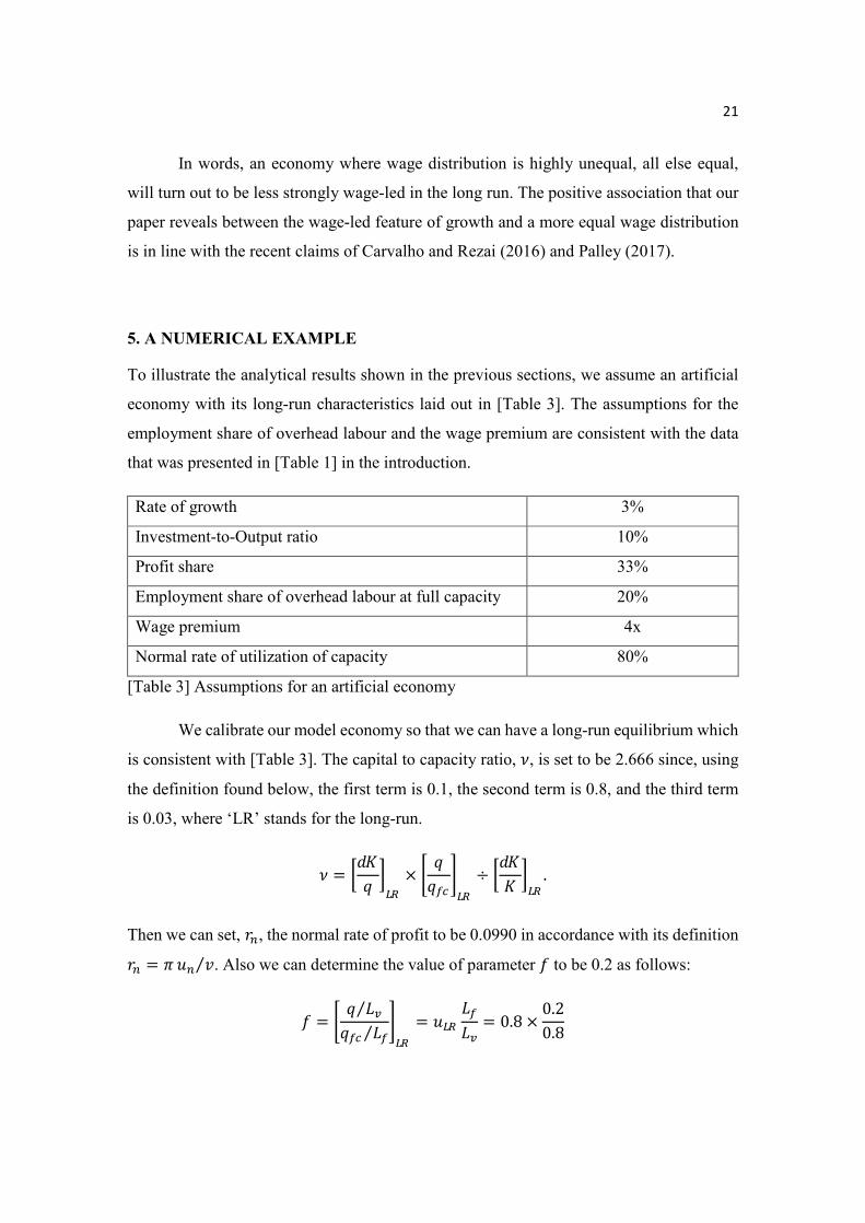
5. A NUMERICAL EXAMPLE
To illustrate the analytical results shown in the previous sections, we assume an artificial
economy with its long-run characteristics laid out in [Table 3]. The assumptions for the
employment share of overhead labour and the wage premium are consistent with the data
that was presented in [Table 1] in the introduction.
Rate of growth 3%
Investment-to-Output ratio 10%
Profit share 33%
Employment share of overhead labour at full capacity 20%
Wage premium 4x
Normal rate of utilization of capacity 80%
[Table 3] Assumptions for an artificial economy
We calibrate our model economy so that we can have a long-run equilibrium which
is consistent with [Table 3]. The capital to capacity ratio, , is set to be 2.666 since, using
the definition found below, the first term is 0.1, the second term is 0.8, and the third term
is 0.03, where ‘LR’ stands for the long-run.
= × ÷ . Then we can set, , the normal rate of profit to be 0.0990 in accordance with its definition = ⁄ . Also we can determine the value of parameter to be 0.2 as follows:
= ⁄ ⁄ = = 0.8 × 0.20.8
22
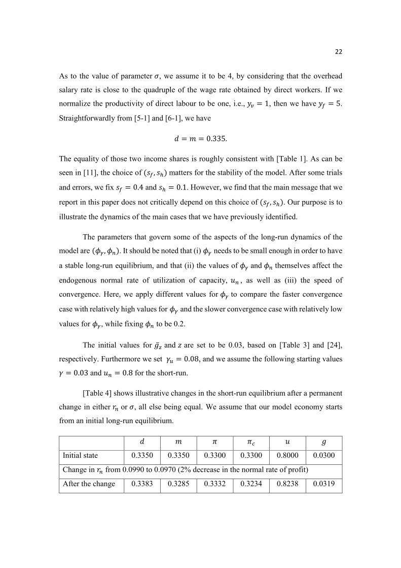
As to the value of parameter , we assume it to be 4, by considering that the overhead
salary rate is close to the quadruple of the wage rate obtained by direct workers. If we
normalize the productivity of direct labour to be one, i.e., = 1, then we have = 5.
Straightforwardly from [5-1] and [6-1], we have = = 0.335. The equality of those two income shares is roughly consistent with [Table 1]. As can be
seen in [11], the choice of (, ) matters for the stability of the model. After some trials
and errors, we fix = 0.4 and = 0.1. However, we find that the main message that we
report in this paper does not critically depend on this choice of (, ). Our purpose is to
illustrate the dynamics of the main cases that we have previously identified.
The parameters that govern some of the aspects of the long-run dynamics of the
model are (, ). It should be noted that (i) needs to be small enough in order to have
a stable long-run equilibrium, and that (ii) the values of and themselves affect the
endogenous normal rate of utilization of capacity, , as well as (iii) the speed of
convergence. Here, we apply different values for to compare the faster convergence
case with relatively high values for and the slower convergence case with relatively low
values for , while fixing to be 0.2.
The initial values for and are set to be 0.03, based on [Table 3] and [24],
respectively. Furthermore we set = 0.08, and we assume the following starting values = 0.03 and = 0.8 for the short-run.
[Table 4] shows illustrative changes in the short-run equilibrium after a permanent
change in either or , all else being equal. We assume that our model economy starts
from an initial long-run equilibrium.
Initial state 0.3350 0.3350 0.3300 0.3300 0.8000 0.0300
Change in from 0.0990 to 0.0970 (2% decrease in the normal rate of profit)
After the change 0.3383 0.3285 0.3332 0.3234 0.8238 0.0319
23
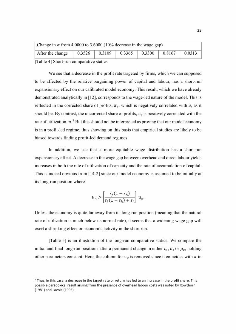
Change in from 4.0000 to 3.6000 (10% decrease in the wage gap)
After the change 0.3526 0.3109 0.3365 0.3300 0.8167 0.0313
[Table 4] Short-run comparative statics
We see that a decrease in the profit rate targeted by firms, which we can supposed
to be affected by the relative bargaining power of capital and labour, has a short-run
expansionary effect on our calibrated model economy. This result, which we have already
demonstrated analytically in [12], corresponds to the wage-led nature of the model. This is
reflected in the corrected share of profits, , which is negatively correlated with , as it
should be. By contrast, the uncorrected share of profits, , is positively correlated with the
rate of utilization, .7 But this should not be interpreted as proving that our model economy
is in a profit-led regime, thus showing on this basis that empirical studies are likely to be
biased towards finding profit-led demand regimes
In addition, we see that a more equitable wage distribution has a short-run
expansionary effect. A decrease in the wage gap between overhead and direct labour yields
increases in both the rate of utilization of capacity and the rate of accumulation of capital.
This is indeed obvious from [14-2] since our model economy is assumed to be initially at
its long-run position where
> (1 − )(1 − ) + . Unless the economy is quite far away from its long-run position (meaning that the natural
rate of utilization is much below its normal rate), it seems that a widening wage gap will
exert a shrinking effect on economic activity in the short run.
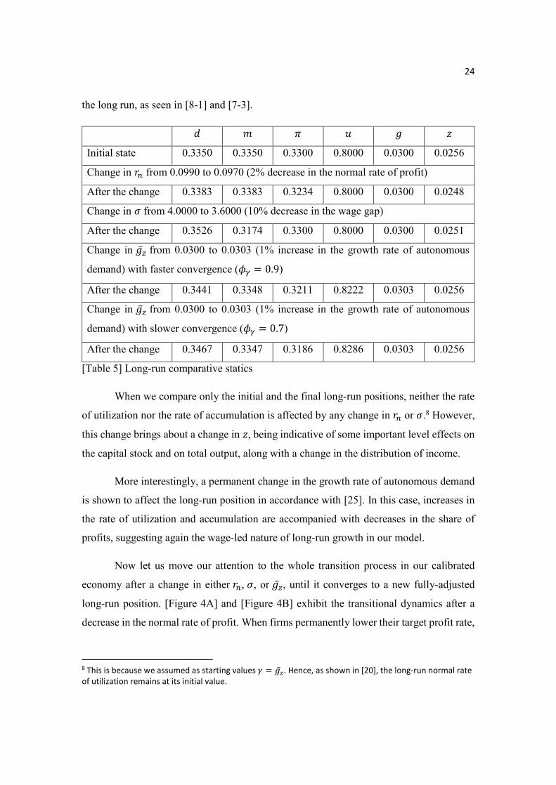
[Table 5] is an illustration of the long-run comparative statics. We compare the
initial and final long-run positions after a permanent change in either , , or , holding
other parameters constant. Here, the column for is removed since it coincides with in
7 Thus, in this case, a decrease in the target rate or return has led to an increase in the profit share. This possible paradoxical result arising from the presence of overhead labour costs was noted by Rowthorn (1981) and Lavoie (1995).
24
the long run, as seen in [8-1] and [7-3].
Initial state 0.3350 0.3350 0.3300 0.8000 0.0300 0.0256
Change in from 0.0990 to 0.0970 (2% decrease in the normal rate of profit)
After the change 0.3383 0.3383 0.3234 0.8000 0.0300 0.0248
Change in from 4.0000 to 3.6000 (10% decrease in the wage gap)
After the change 0.3526 0.3174 0.3300 0.8000 0.0300 0.0251
Change in from 0.0300 to 0.0303 (1% increase in the growth rate of autonomous
demand) with faster convergence ( = 0.9)
After the change 0.3441 0.3348 0.3211 0.8222 0.0303 0.0256
Change in from 0.0300 to 0.0303 (1% increase in the growth rate of autonomous
demand) with slower convergence ( = 0.7)
After the change 0.3467 0.3347 0.3186 0.8286 0.0303 0.0256
[Table 5] Long-run comparative statics
When we compare only the initial and the final long-run positions, neither the rate
of utilization nor the rate of accumulation is affected by any change in or .8 However,
this change brings about a change in , being indicative of some important level effects on
the capital stock and on total output, along with a change in the distribution of income.
More interestingly, a permanent change in the growth rate of autonomous demand
is shown to affect the long-run position in accordance with [25]. In this case, increases in
the rate of utilization and accumulation are accompanied with decreases in the share of
profits, suggesting again the wage-led nature of long-run growth in our model.
Now let us move our attention to the whole transition process in our calibrated
economy after a change in either , , or , until it converges to a new fully-adjusted
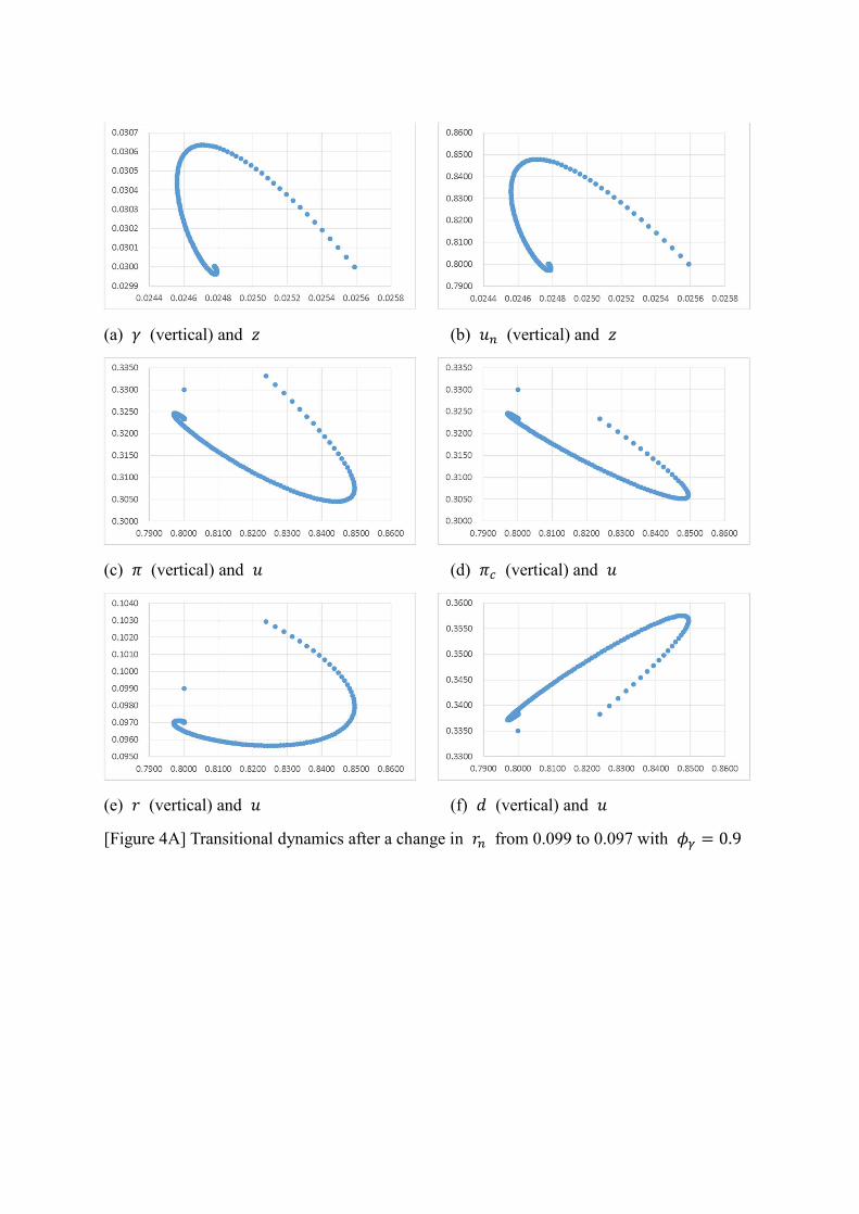
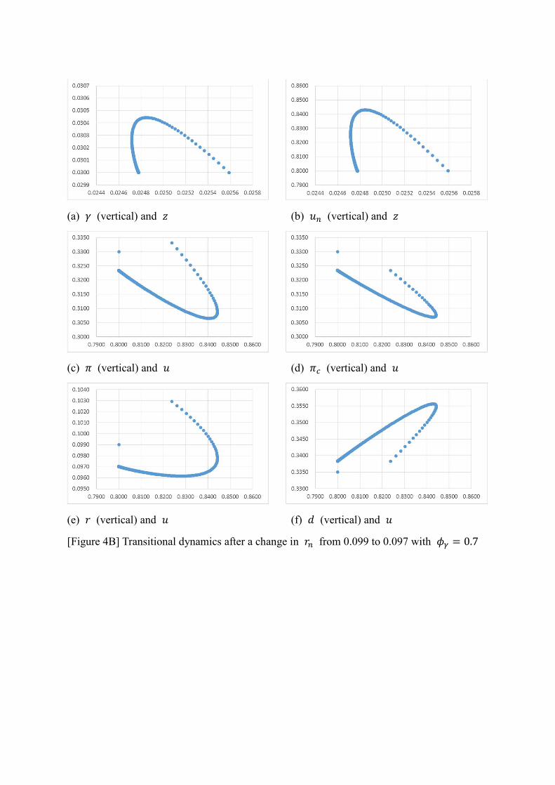
long-run position. [Figure 4A] and [Figure 4B] exhibit the transitional dynamics after a
decrease in the normal rate of profit. When firms permanently lower their target profit rate,
8 This is because we assumed as starting values = . Hence, as shown in [20], the long-run normal rate of utilization remains at its initial value.
25
we see that the rate of utilization stays at a higher level than its initial normal rate for a
while and then gradually comes back to its initial normal rate in the long run.
[Figure 4A] around here
[Figure 4B] around here
One thing that stands out is that we generate here a clockwise loop in (, ) space.
Also, it seems that whether the share of profits is corrected or not matters in accounting for
the very early phase of expansion. The uncorrected one, , increases initially, and this at
first glance seems to indicate that an increase in contributes to an initial increase in the
rate of profit together with an increase in the rate of utilization. However, the corrected one, , does not go up when the economy expands as we can see in (d). We know that, if
increases while does not, then this increase in is solely due to an increase in the rate
of utilization. Thus, comparing (c) and (d), we can conclude that the increase in the rate of
profit during the initial expansionary phase reflects the increase in effective demand caused
by the decrease in the target rate return of firms, which could arise as a consequence of the
strengthening bargaining power of labour unions or as the consequence of foreign
competition.
[Figure 4C] and [Figure 4D] exhibit the long-run level effects on the capital stock
and output of a permanent decrease in . The graph describes the level of capital and
output relative to the case of no change in . For instance, when = 0.9, the long-run
output level with = 0.097 is around 3% higher than the one with = 0.099 under the
current calibration. Apparently, the increase in the relative bargaining position of workers,
which may result in a decrease in the normal rate of profit, seems to have a long-run
expansionary effect on the economy.
[Figure 4C] around here
[Figure 4D] around here
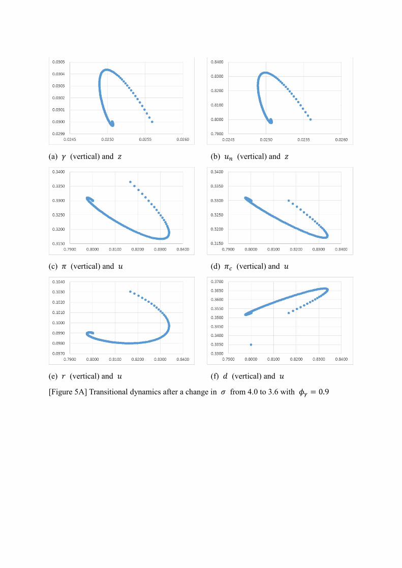
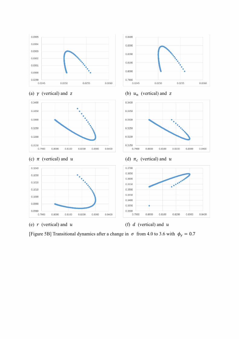
[Figure 5A] and [Figure 5B] show the transitional dynamics after a decrease in the
wage premium. We can see that the rate of utilization initially increases and then comes
back to its initial level in the long run. Once more, despite the wage-led nature of our model
26
economy, the change generates a clockwise loop in (, ) space. The initial increase in the
rate of profit in the early expansion is entirely due to the increase in the rate of utilization.
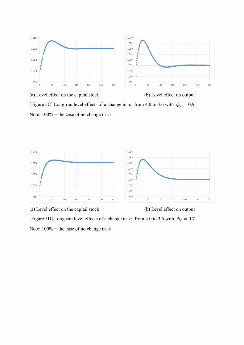
[Figure 5C] and [Figure 5D] also illustrate the positive level effects of a more equitable
wage distribution on the capital stock and on output.
[Figure 5A] around here
[Figure 5B] around here
[Figure 5C] around here
[Figure 5D] around here
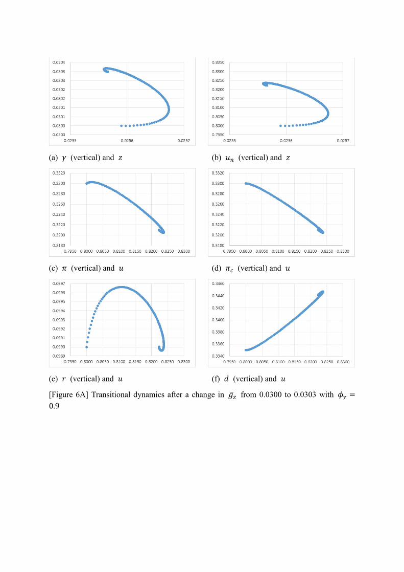
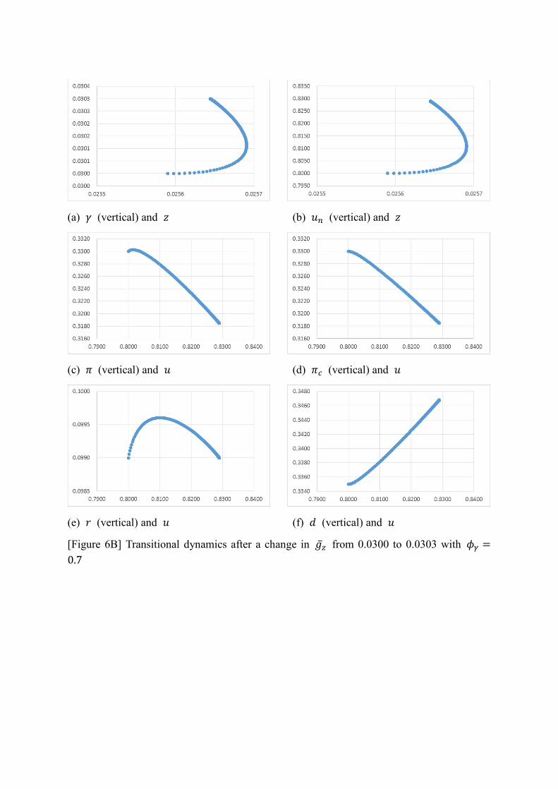
Finally, [Figure 6A], [Figure 6B], [Figure 6C] and [Figure 6D] illustrate the case
of a permanent increase in the growth rate of autonomous consumption. Such a change
generates an increase in the rate of capacity utilization and a fall in the profit share. It is
particularly interesting to note that the faster growth rate of autonomous consumption
generates a dynamic evolution of the profit rate relative to the rate of utilization that takes
a bell shape when the profit rate is measured on the vertical axis. This dynamic bell-shaped
relationship is remindful of the shape of the so-called distributive curve assumed by a
variety of authors, who argued, on the basis of observed behaviour, that there would be a
positive relationship between the profit rate and the rate of utilization at low rates of
utilization, and a negative relationship at high rates of utilization, thus claiming that the
economy would be wage led at low rates of utilization and profit led at high rates (Gordon
1994, 152; You 1994, 222; Nikiforos and Foley 2012). Here the profit rate is fully
endogenous and its bell-shaped evolution is not caused by any change in the bargaining
position of the various income classes.
[Figure 6A] around here
[Figure 6B] around here
[Figure 6C] around here
[Figure 6D] around here
27
6. CONCLUSION
We have devised a neo-Kaleckian model of growth and distribution where capital
accumulation depends on the expected growth rate of sales and on the discrepancy between
the actual and the normal rate of capacity utilization, but where the economy is driven by
the growth rate of autonomous non-capacity creating expenditures, more specifically by
the growth rate of autonomous consumption expenditures, those that Fiebiger (2018a) calls
semi-autonomous household expenditures.
There are three novel features in the present model. First, we distinguish between
managerial labour – white-collar or supervisory workers, the working rich – on the one
hand, and direct labour – blue-collar or non-supervisory workers, the working poor – on
the other hand. Blue-collar workers do not save, whereas white-collar workers have a given
marginal propensity to save out of their salaries and out of the capital income they receive
from firms. The white-collar workers are the social class that has autonomous consumption
expenditures. The saving function is thus more complex than usual in this kind of model.
The employment of direct labour moves proportionately with the level of actual
output whereas the employment of managers is tied to the level of full-capacity output. In
accordance with the stylized facts noted in the introduction, there is a substantial
differential between the wage rate received by managers compared to that obtained by non-
supervisory workers. It follows that the profit share becomes an endogenous variable,
which is a positive function of the level of capacity utilization, as is often observed in the
early phase of the business cycle.
The second innovative feature of our model is that we suppose that firms set prices
on the basis of a target-return pricing formula. As a consequence, an increase in the wage
rate of supervisory workers relative to that of non-supervisory workers will lead to an
increase in the mark-up set by firms, thus modifying in general the income distribution
between profits and wages, as well as the distribution between wages going to managers
and wages going to direct workers.
28
The third innovation of the present model with autonomous consumption
expenditures is that in the long run we assume the combination of two adjustment
mechanisms. As done in previous neo-Kaleckian models with autonomous non-capacity
creating expenditures, we introduce a slow Harrodian instability mechanism, whereby
firms increase the expected growth rate of sales when the actual growth rate is above the
one expected by firms. The second long-run adjustment mechanism concerns the normal
rate of utilization, which plays a role both in the investment function and in the pricing
formula. It is assumed that the normal rate of capacity utilization is a convention, and that
this normal rate of utilization will tend to slowly increase whenever the realized rates of
utilization will surpass the normal rate.
Several interesting results directly arise from the target-return pricing formula
combined to the distinction between supervisory and non-supervisory workers. First an
increase the target rate of return or in the relative real wage of supervisory workers, at a
given rate of capacity utilization, leads to a fall in the income share of non-supervisory
workers. Second, at a given rate of capacity utilization, this increase in the relative real
wage of supervisory workers will lead to an increase (decrease) in the profit share if this
given actual rate of capacity utilization is bigger (smaller) than the normal rate.
Third, in an economy with overhead labour, all else equal, that is, with no change
whatsoever in the mark-up over unit direct labour costs, an increase in the rate of utilization
leads to a fall in the share of managerial income and an increase in the share of profits.
Thus, unless the measures of the profit share are corrected for this effect, statistical
enquiries will be biased towards finding that the aggregate demand regime is profit-led.
We have computed an amended version of the corrected profit share suggested by
Weisskopf (1979), where the share of managers is corrected by the actual rate of utilization
relative to the normal rate, and have shown that this measure is both impervious to a change
in the actual rate of capacity utilization and in the wage differential between supervisory
and non-supervisory workers, as it ought to be when firms use a target-return pricing
formula.
Combining now the above supply-side and demand-side effects, we have shown
that in the short run an increase in the bargaining power of firms as reflected by their target
29
rate of return always leads to a fall in the equilibrium rate of capacity utilization and in the
rate of accumulation. The model is thus wage-led in the short run. We have also identified
the conditions under which an increase in the wage differential favouring supervisory
workers will lead in the short run to a fall in the rate of capacity utilization and in the rate
of accumulation. This will necessarily occur when the actual rate of utilization is higher
than the normal rate of utilization, but it may also happen if the actual rate of utilization is
smaller than the normal rate of utilization, provided the actual rate is greater than a certain
fraction of the normal rate. This fraction depends on the retention ratio of firms and on the
marginal propensity to save of rich households. The higher is this marginal propensity to
save of supervisory workers, the smaller will that fraction be, and hence the more likely it
is that more inequality in the distribution of wages will generate lower rates of utilization
and of accumulation. This result is intuitive because the redistribution of income from non-
supervisory workers, who do not save, towards supervisory workers, who do save, will
reduce aggregate demand, so this negative effect will be particularly strong if the marginal
propensity to save of supervisory workers is high.
As to the effect of a redistribution of income towards overhead labour on the short-
run equilibrium profit share, we have shown that its effect is particularly uncertain. The
only thing that can be said with certainty is that if the actual rate of utilization is in-between
the same fraction of the normal rate of utilization evoked above and the normal rate of
utilization, then more wage inequality will generate a fall in the short-run equilibrium value
of the profit share.
Finally we consider the results obtained for the long-run equilibrium of the model.
The two adjustment mechanisms involving the expected growth rate of sales (the Harrodian
instability mechanism) and the normal rate of capacity utilization, combined with the
dynamic behaviour of the relative weight of the autonomous consumption expenditures,
drive the economy towards a fully-adjusted state, at a normal rate of capacity utilization,
provided the Keynesian short-run stability condition holds and provided Harrodian
instability is not overly strong. The system of dynamic equations is however path
dependent so that the long-run solution depends on the initial conditions of the model as
well as on the strength of the adjustment mechanisms during the transition – an interesting
30
case of hysteresis. This is what Setterfield (1993) calls a case of deep endogeneity.
We have shown that an increase in the target rate of return set by firms leads to a
fall in the average growth rate during the traverse to the new long-run equilibrium – a result
which is consistent with what we had observed in the short run. The economy is thus clearly
wage led, a result which is not really surprising given the formulation of the investment
function, given by equation [10], which does not include a term ascertaining expected
profitability (at the normal rate of capacity utilization), in contrast to the post-Kaleckian
model of Bhaduri and Marglin (1990).
What is more surprising and particularly interesting in the study of the long-run
effects of our model is that, despite the ambiguous short-run effect on the rate of capacity
utilization and the rate of accumulation of an increase in the wage differential favouring
supervisory workers, there is no ambiguity with respect to the long-run effect. We have
demonstrated that increased inequality in wage distribution necessarily leads to a fall in the
average rate of growth of the economy during the traverse from the old to the new long-
run equilibrium, thus implying a lower level of economic activity and lower potential
output in the long run compared to a situation with no change in wage dispersion.
All of the above algebraic results have been verified with simulations on a
calibrated version of our algebraic model. In particular, the cyclical behaviour of our model
has been shown in both cases of slow and fast adjustments. Despite the wage-led nature of
our model economy, an increase in the target profit rate or in the share of wages going to
supervisory workers generates a clockwise loop in (, ) space, a kind of loop which is
usually associated with a Goodwin model, with its profit-led demand regime combined to
a profit-squeeze distributive curve. This is reminiscent of the apparent Goodwin cycles
generated by Minskyan debt effects, as shown by Stockhammer and Michell (2017).
The main implication of these results, if the model is sufficiently faithful to reality,
is that governments should pursue policies that tend to reduce wage dispersion between
managerial jobs and non-supervisory jobs, as Palley (2017) also concludes. This calls for
a return to egalitarian wage policies or solidarity wage policies. In other words, besides the
possibility of a wage-led growth regime, our long-run results provide support for a growth
31
strategy based on wage equality and the imposition of constraints on the perks and salaries
obtained by executive managers, such as the imposition of a maximum ratio between
executive income and the average or medium wage of the other employees of a firm.
32
REFERENCES
Allain, O. (2015), ‘Tackling the instability of growth: a Kaleckian-Harrodian model with an autonomous expenditure component’, Cambridge Journal of Economics, 39 (5), 1351-1371.
Allain, O. (2018), ‘Demographic growth, Harrodian (in)stability and the supermultiplier’, Cambridge Journal of Economics, Advanced access, https://doi.org/10.1093/cje/bex082
Amadeo, E.J. (1986), ‘Notes on capacity utilization, distribution and accumulation’, Contributions to Political Economy, 5 (1), March, 83-94.
Asimakopulos, A. (1970), ‘A Robinsonian growth model in one-sector notation – an amendment’, Australian Economic Papers, December, 171-176.
Bhaduri, A. and S. Marglin (1990), ‘Unemployment and the real wage: the economic basis for contesting political ideologies’, Cambridge Journal of Economics, 14 (4), December, 375-393.
Carvalho, L. and A. Rezai (2016), ‘Personal income inequality and aggregate demand’, Cambridge Journal of Economics, 40 (2), 491-505.
Cassetti, M. (2006) ‘A note on the long-run behaviour of Kaleckian models’, Review of Political Economy, 18 (4), October, 497-508.
Ciccone, R. (1986), ‘Accumulation and capacity utilization: some critical considerations on Joan Robinson's theory of distribution’, Political Economy: Studies in the Surplus Approach, 2 (1), 17-36.
Dávila-Fernández, M.J., Oreiro, J.L., and Punzo, L.F. (2017). Inconsistency and over-determination in neo-Kaleckian growth models: A note. Metroeconomica, Advanced access, doi.org/10.1111/meca.12190
Dutt, A.K. (1997), ‘Equilibrium, path dependence and hysteresis in post-Keynesian models’, in P. Arestis, G. Palma and M. Sawyer (eds), Markets, Unemployment and Economic Policy: Essays in Honour of Geoff Harcourt, Volume Two, London: Routledge, pp. 238-253.
Dutt, A.K. (2012): Growth, distribution and crises, in: H. Herr, T. Niechoj, C. Thomasberger, A. Truger and T. van Treeck (eds), From Crisis to Growth? The Challenge of Debt and Imbalances, Metropolis, Marburg, 33-59.
Dutt, A. K. (2015), ‘Growth and distribution with exogenous autonomous demand growth and normal capacity utilization’, Workshop on Analytical Political Economy, Tohoku University, Sendai, Japan.
Fazzari, S., P. Ferri and A.M. Variato (2018), ‘Demand-led growth and accommodating supply’, FFM Working paper No 15, Hans-Böckler-Stiftung.
33
Fiebiger, B. (2018a), ‘Semi-autonomous household expenditures as the causa causans of postwar US business cycles: the stability and instability of Luxemburg-type external markets’, Cambridge Journal of Economics, 42 (1), 155-175.
Fiebiger, B. (2018b), ‘Some suggestions on endogeneity in the normal rate of capacity utilization’, mimeo, July 2018.
Freitas, F. and F. Serrano (2015), ‘Growth rate and level effects: the stability of the adjustment of capacity to demand and the Sraffian supermultiplier’, Review of Political Economy, 27 (3), 258-281.
Gordon, D.M. (1994), ‘Putting heterodox macro to the test: comparing post-Keynesian, Marxian, and Social Structuralist macroeconometric models of the post-war US economy’, in M.A. Glick (ed.), Competition, Technology and Money: Classical and Post-Keynesian Perspectives, Cheltenham: Edward Elgar, pp. 143-185.Harris, D.J. (1974), ‘The price policy of firms, the level of employment and distribution of income in the short run’, Australian Economic Papers, 13 (22), June, 144-151.
Hein, E. (2018), ‘Autonomous government expenditure growth, deficits, debt and distribution in a neo-Kaleckian growth model’, Journal of Post Keynesian Economics, 41 (2), 316-338.
Hein, E., M. Lavoie, and T. Van Treeck (2012), ‘Harrodian instability and the normal rate of capacity utilization in Kaleckian models of distribution and growth – a survey’, Metroeconomica, 63 (1), 39-69.
Kurz, H.D. (1990), ‘Technical change, growth and distribution: A steady state approach to unsteady growth’, in Kurz, H.D., Capital, Distribution and Effective Demand: Studies in the Classical Approach to Economic Theory, Cambridge: Polity Press, pp. 210-239.
Lavoie, M. (1992), Foundations of Post-Keynesian Economic Analysis, Edward Elgar: Aldershot.
Lavoie, M. (1995), ‘The Kaleckian model of growth and distribution and its neo-Ricardian and neo-Marxian critiques’, Cambridge Journal of Economics, 19 (6), 789-818.
Lavoie, M. (1996a), ‘Unproductive outlays and capital accumulation with target-return pricing’, Review of Social Economy, 54 (3), Fall, 303-321.
Lavoie, M. (1996b), ‘Traverse, hysteresis, and normal rates of capacity utilization in Kaleckian models of growth and distribution, Review of Radical Political Economics, 28 (4), 113-147.
Lavoie, M. (2009), ‘Cadrisme within a Kaleckian model of growth and distribution’, Review of Political Economy, 21 (3), July, 371-393.
Lavoie, M. (2010), ‘Surveying long-run and short-run stability issues with the Kaleckian model of growth’, in Setterfield, M. (ed.): Handbook of Alternative Theories of Economic Growth, Edward Elgar, Cheltenham.
Lavoie, M. (2014), Post-Keynesian Economics: New Foundations, Cheltenham: Edward Elgar.
34
Lavoie, M. (2016), ‘Convergence towards the normal rate of capacity utilization in neo-Kaleckian models: The role of non-capacity creating autonomous expenditures’, Metroeconomica, 67 (1), 172-201.
Lavoie, M. (2017), ‘The origins and evolution of the debate on wage-led and profit-led regimes’, European Journal of Economics and Economic Policies: Intervention, 14 (2), 200-221.
Lavoie, M., Rodríguez, G., Seccareccia, M. (2004), ‘Similitudes and discrepancies in post-Keynesian and Marxist theories of investment: A theoretical and empirical investigation’, International Review of Applied Economics, 18 (2), 127-149.
Lavoie, M., Stockhammer, E. (2013), Wage-led Growth: An Equitable Strategy for Economic Recovery, Basingstoke: Palgrave Macmillan.
Lee, F.S. (1998), Post Keynesian Price Theory, Cambridge: Cambridge University Press.
Lee, F.S. (2013), ‘Post-Keynesian price theory’, in Harcourt, G.C. and Kriesler, P. (eds), The Oxford Handbook of Post-Keynesian Economics: Volume I: Theory and Origins, Oxford: Oxford University Press, pp. 467-484.
Mohun, S. (2014), ‘Unproductive labor in the U.S. economy: 1964-2010’, Review of Radical Political Economics, 46 (3), 355-379.
Nah, W.J. and M. Lavoie (2017), ‘Long-run convergence in a neo-Kaleckian open-economy model with autonomous export growth’, Journal of Post Keynesian Economics, 40 (2), 223-238.
Nah, W.J. and M. Lavoie (2018a), ‘Convergence in a neo-Kaleckian model with endogenous technical progress and autonomous demand growth’, Review of Keynesian Economics, forthcoming.
Nah, W.J. and M. Lavoie (2018b), ‘The role of autonomous demand growth in a neo-Kaleckian conflicting-claims framework’, FMM working paper, https://www.boeckler.de/pdf/p_fmm_imk_wp_22_2018.pdf
Nichols, L.M. and N. Norton (1991), ‘Overhead workers and political economy macro models’, Review of Radical Political Economy, 23 (1-2), Spring-Summer, 47-54.
Nikiforos, M. (2016), ‘On the utilization controversy: A theoretical and empirical discussion of the Kaleckian model of growth and distribution’, Cambridge Journal of Economics, 40 (2), 437-467.
Nikiforos, M. (2017), ‘Uncertainty and contradiction: An essay on the business cycle’, Review of Radical Political Economics, 49 (2), 247-264.
Nikiforos, M. and Foley, D.K. (2012), ‘Distribution and capacity utilization: conceptual issues and empirical evidence’, Metroeconomica, 63 (1), 200-229.
35
Palley, T.I. (2015), ‘The middle class in macroeconomics and growth theory: a three-class neo-Kaleckian-Goodwin model’, Cambridge Journal of Economics, 39 (1), 221-243.
Palley, T.I. (2017), ‘Wage- vs profit-led growth: the role of the distribution of wages in determining regime character’, Cambridge Journal of Economics, 41 (1), 49-61.
Piketty, T. (2014), Capital in the Twenty-First Century, Cambridge (Mass.): Harvard University Press.
Rolim, L.N. (2017), ‘Overhead labour and feedback effects between capacity utilization and income distributions: Estimations for the USA economy’, https://www.boeckler.de/pdf/v_2017_11_10_nogueira_rolim.pdf
Rowthorn, B. (1981), ‘Demand, real wages and economic growth’, Thames Papers in Political Economy, Autumn, 1-39.
Schoder, C. (2012), ‘Endogenous capital productivity in the Kaleckian growth models: theory and evidence’, available at http://www.boeckler.de/pdf/p_imk_wp_102_2012.pdfhttp://www.boeckler.de/pdf/p_imk_wp_102_2012.pdf
Setterfield, M. (1993): Towards a long-run theory of effective demand: Modelling macroeconomic systems with hysteresis, Journal of Post Keynesian Economics, 15 (3), 347-364.
Setterfield, M. (2017): Long-run variations in the rate of capacity utilization in the presence of a fixed normal rate, Working paper 1704, Department of Economics, New School for Social Research.
Sherman, H.J., Evans, G.R. (1984): Macro-Economics: Keynesian, Monetarist and Marxist Views, New York: Harper & Row.
Stockhammer, E. and Michell, J. (2017), ‘Pseudo-Goodwin cycles in a Minsky model’, Cambridge Journal of Economics, 41 (1), 105-125.
Tavani, D., Petach, L. (2018), ‘No one is alone: strategic complementarities, capacity utilization, growth, and distribution’. FMM working papers, https://www.boeckler.de/pdf/p_fmm_imk_wp_19_2018.pdf
Tavani, D., Vasaudevan, R. (2014), ‘Capitalists, workers, and managers: Wage inequality and effective demand’, Structural Dynamics and Economic Change, 30 (1), 120-131.
Weisskopf, T.E. (1979), ‘Marxian crisis theory and the rate of profit in the postwar U.S. economy’, Cambridge Journal of Economics, 3(4), 341-378.
You, J.I. (1994), ‘Macroeconomic structures, endogenous technical change and growth’, Cambridge Journal of Economics, 18 (2), 213-233.
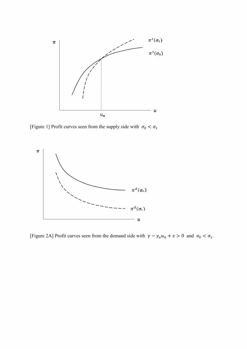
[Figure 1] Profit curves seen from the supply side with <
[Figure 2A] Profit curves seen from the demand side with − + > 0 and < .
() ()
()
()
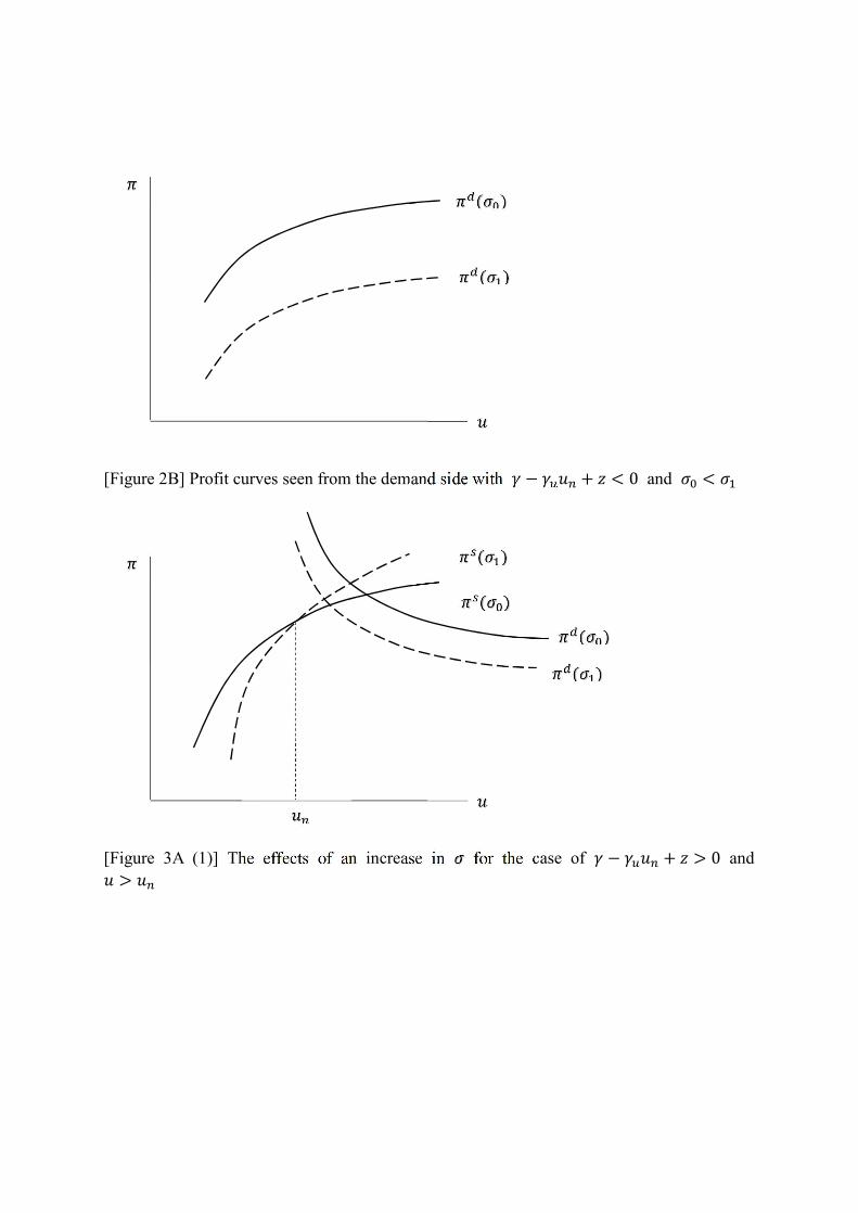
[Figure 2B] Profit curves seen from the demand side with − + < 0 and <
[Figure 3A (1)] The effects of an increase in for the case of − + > 0 and >
() ()
() ()
() ()
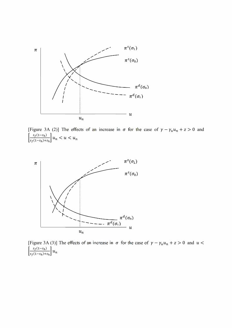
[Figure 3A (2)] The effects of an increase in for the case of − + > 0 and ()() < <
[Figure 3A (3)] The effects of an increase in for the case of − + > 0 and < ()()
() ()
() ()
() ()
() ()
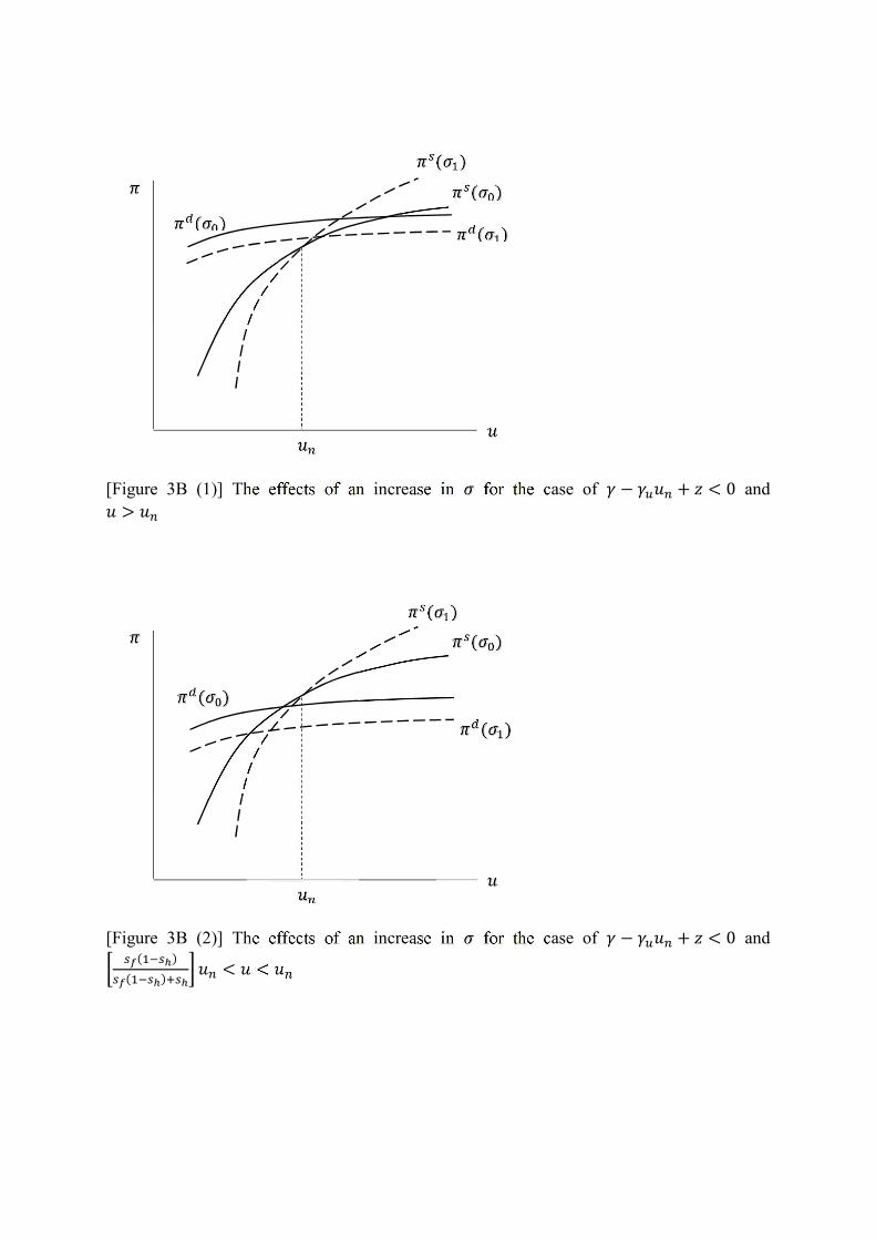
[Figure 3B (1)] The effects of an increase in for the case of − + < 0 and >
[Figure 3B (2)] The effects of an increase in for the case of − + < 0 and ()() < <
() ()
() ()
()
() () ()
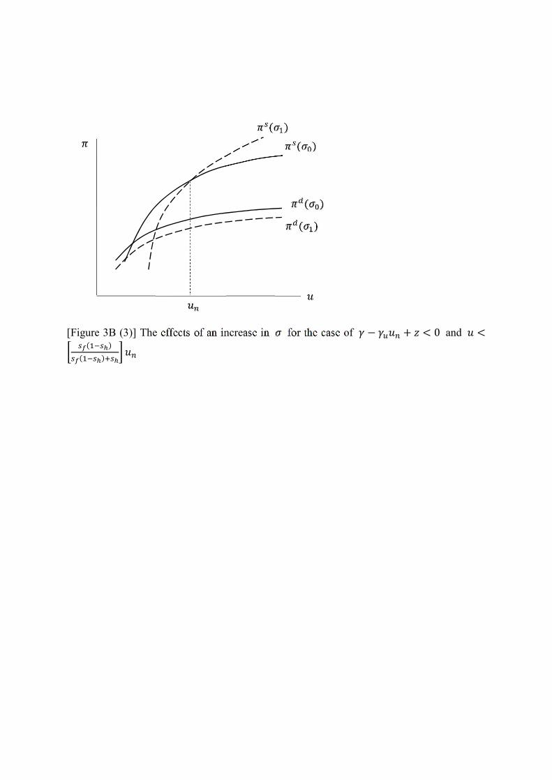
[Figure 3B (3)] The effects of an increase in for the case of − + < 0 and < ()()
()
() ()
()
(a) (vertical) and (b) (vertical) and
(c) (vertical) and (d) (vertical) and
(e) (vertical) and (f) (vertical) and
[Figure 4A] Transitional dynamics after a change in from 0.099 to 0.097 with = 0.9
(a) (vertical) and (b) (vertical) and
(c) (vertical) and (d) (vertical) and
(e) (vertical) and (f) (vertical) and
[Figure 4B] Transitional dynamics after a change in from 0.099 to 0.097 with = 0.7
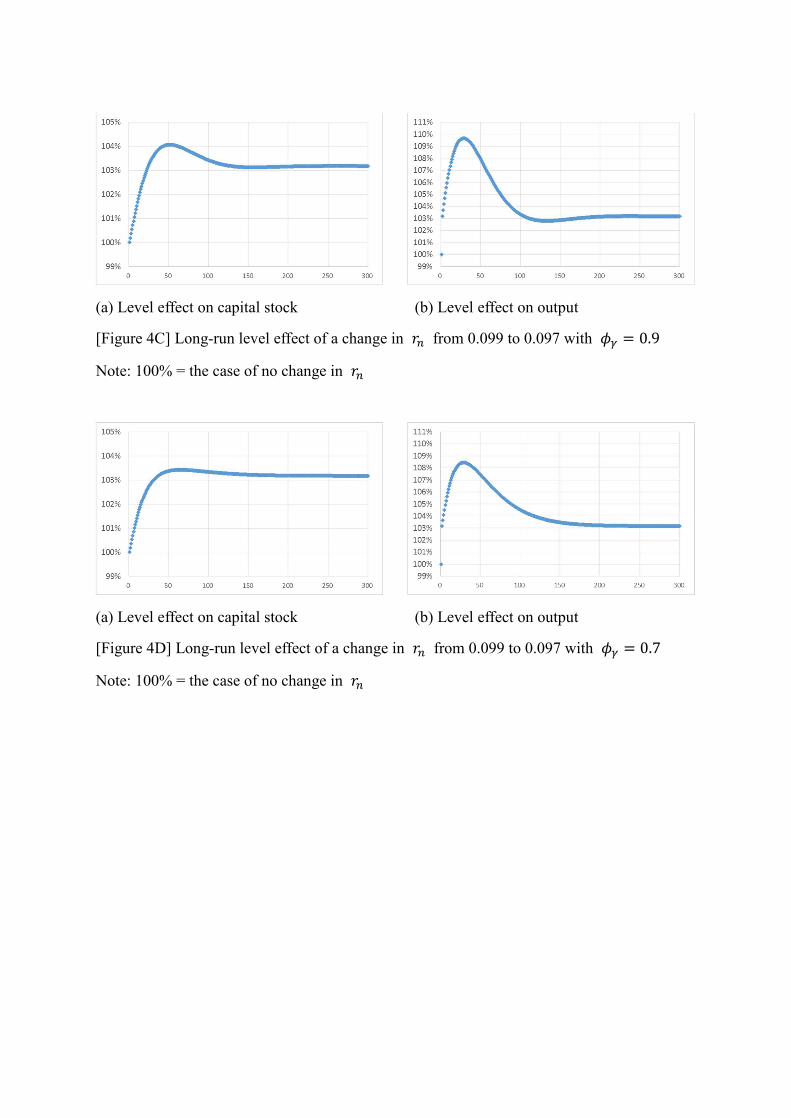
(a) Level effect on capital stock (b) Level effect on output
[Figure 4C] Long-run level effect of a change in from 0.099 to 0.097 with = 0.9
Note: 100% = the case of no change in
(a) Level effect on capital stock (b) Level effect on output
[Figure 4D] Long-run level effect of a change in from 0.099 to 0.097 with = 0.7
Note: 100% = the case of no change in
(a) (vertical) and (b) (vertical) and
(c) (vertical) and (d) (vertical) and
(e) (vertical) and (f) (vertical) and
[Figure 5A] Transitional dynamics after a change in from 4.0 to 3.6 with = 0.9
(a) (vertical) and (b) (vertical) and
(c) (vertical) and (d) (vertical) and
(e) (vertical) and (f) (vertical) and
[Figure 5B] Transitional dynamics after a change in from 4.0 to 3.6 with = 0.7
(a) Level effect on the capital stock (b) Level effect on output
[Figure 5C] Long-run level effects of a change in from 4.0 to 3.6 with = 0.9
Note: 100% = the case of no change in
(a) Level effect on the capital stock (b) Level effect on output
[Figure 5D] Long-run level effects of a change in from 4.0 to 3.6 with = 0.7
Note: 100% = the case of no change in
(a) (vertical) and (b) (vertical) and
(c) (vertical) and (d) (vertical) and
(e) (vertical) and (f) (vertical) and
[Figure 6A] Transitional dynamics after a change in from 0.0300 to 0.0303 with =0.9
(a) (vertical) and (b) (vertical) and
(c) (vertical) and (d) (vertical) and
(e) (vertical) and (f) (vertical) and
[Figure 6B] Transitional dynamics after a change in from 0.0300 to 0.0303 with =0.7
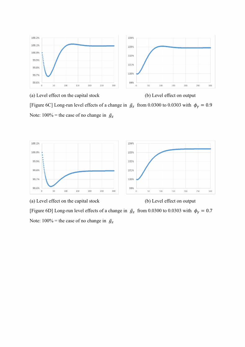
(a) Level effect on the capital stock (b) Level effect on output
[Figure 6C] Long-run level effects of a change in from 0.0300 to 0.0303 with = 0.9
Note: 100% = the case of no change in
(a) Level effect on the capital stock (b) Level effect on output
[Figure 6D] Long-run level effects of a change in from 0.0300 to 0.0303 with = 0.7
Note: 100% = the case of no change in
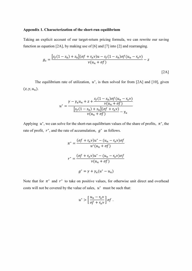
Appendix 1. Characterization of the short-run equilibrium
Taking an explicit account of our target-return pricing formula, we can rewrite our saving
function as equation [2A], by making use of [6] and [7] into [2] and rearranging.
= (1 − ) + ( + ) − (1 − )( − )( + ) −
[2A]
The equilibrium rate of utilization, ∗, is then solved for from [2A] and [10], given (, , ).
∗ = − + + (1 − )( − )( + )(1 − ) + ( + )( + ) −
Applying ∗, we can solve for the short-run equilibrium values of the share of profits, ∗, the
rate of profit, ∗, and the rate of accumulation, ∗ as follows.
∗ = ( + )∗ − ( − )∗( + )
∗ = ( + )∗ − ( − )( + )
∗ = + (∗ − )
Note that for ∗ and ∗ to take on positive values, for otherwise unit direct and overhead
costs will not be covered by the value of sales, ∗ must be such that:
∗ > − + .
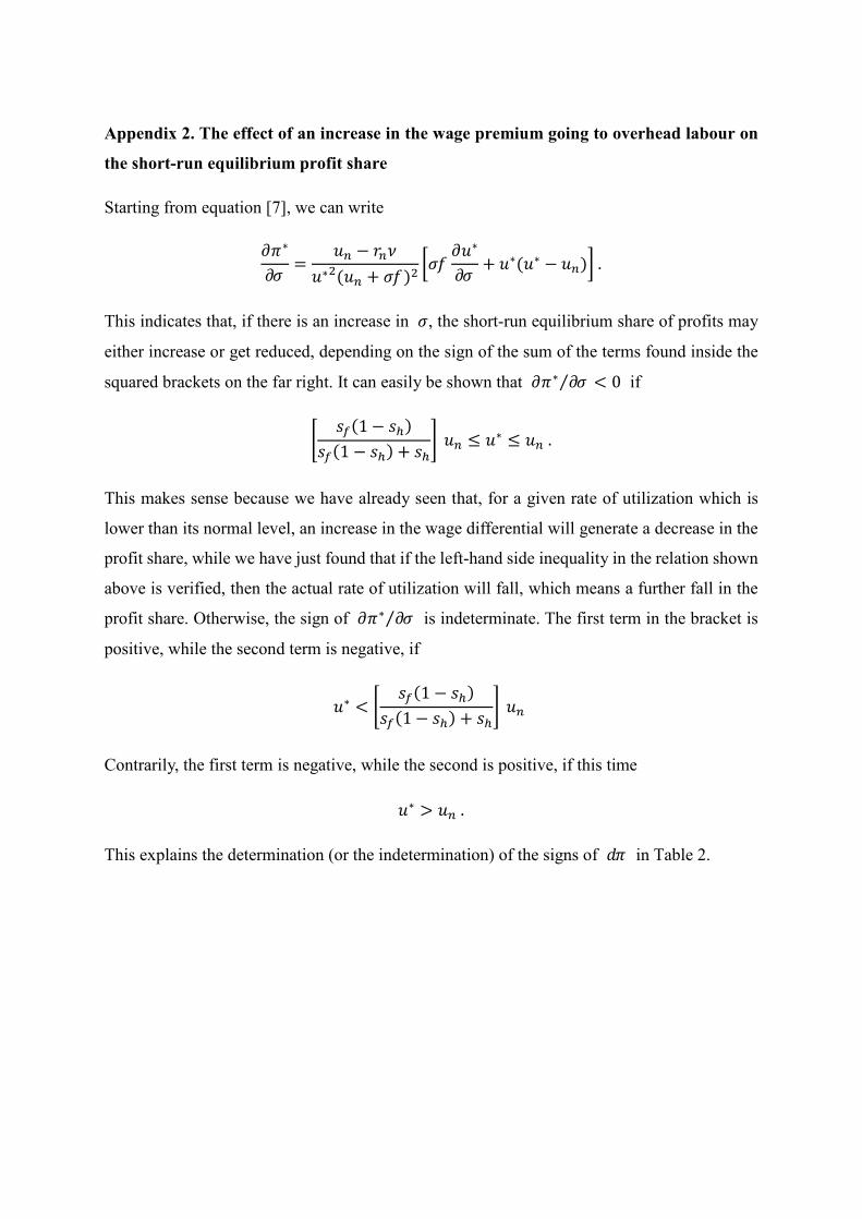
Appendix 2. The effect of an increase in the wage premium going to overhead labour on
the short-run equilibrium profit share
Starting from equation [7], we can write ∗ = − ∗( + ) ∗ + ∗(∗ − ). This indicates that, if there is an increase in , the short-run equilibrium share of profits may
either increase or get reduced, depending on the sign of the sum of the terms found inside the
squared brackets on the far right. It can easily be shown that ∗ ⁄ < 0 if
(1 − )(1 − ) + ≤ ∗ ≤ . This makes sense because we have already seen that, for a given rate of utilization which is
lower than its normal level, an increase in the wage differential will generate a decrease in the
profit share, while we have just found that if the left-hand side inequality in the relation shown
above is verified, then the actual rate of utilization will fall, which means a further fall in the
profit share. Otherwise, the sign of ∗ ⁄ is indeterminate. The first term in the bracket is
positive, while the second term is negative, if
∗ < (1 − )(1 − ) + Contrarily, the first term is negative, while the second is positive, if this time ∗ > . This explains the determination (or the indetermination) of the signs of in Table 2.
Appendix 3. Long-run stability
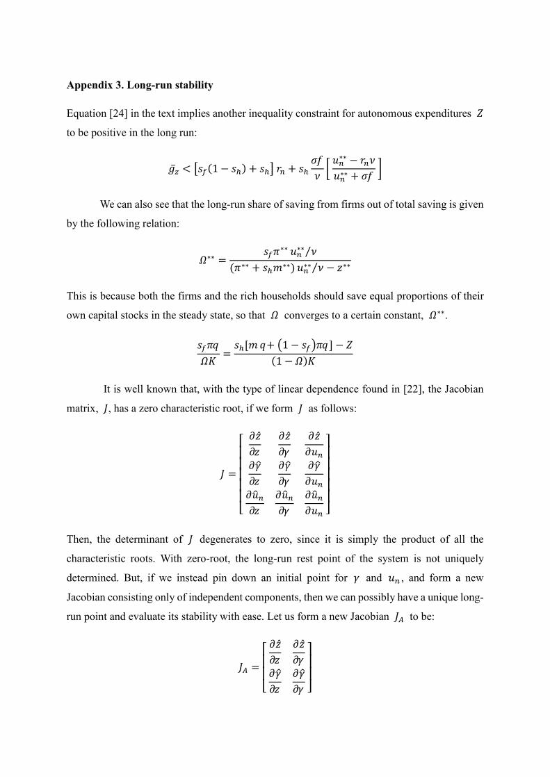
Equation [24] in the text implies another inequality constraint for autonomous expenditures
to be positive in the long run:
< (1 − ) + + ∗∗ − ∗∗ +
We can also see that the long-run share of saving from firms out of total saving is given
by the following relation:
∗∗ = ∗∗ ∗∗ ⁄(∗∗ + ∗∗) ∗∗ ⁄ − ∗∗
This is because both the firms and the rich households should save equal proportions of their
own capital stocks in the steady state, so that converges to a certain constant, ∗∗. = [ + 1 − ] − (1 − )
It is well known that, with the type of linear dependence found in [22], the Jacobian
matrix, , has a zero characteristic root, if we form as follows:
=⎣⎢⎢⎢⎢⎢⎡
⎦⎥⎥⎥⎥⎥⎤
Then, the determinant of degenerates to zero, since it is simply the product of all the
characteristic roots. With zero-root, the long-run rest point of the system is not uniquely
determined. But, if we instead pin down an initial point for and , and form a new
Jacobian consisting only of independent components, then we can possibly have a unique long-
run point and evaluate its stability with ease. Let us form a new Jacobian to be:
= ⎣⎢⎢⎡ ⎦⎥⎥
⎤
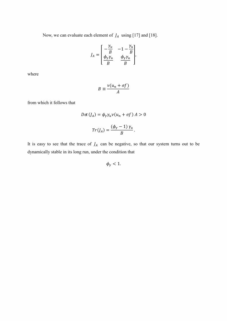
Now, we can evaluate each element of using [17] and [18].
= − −1 − , where
≡ ( + )
from which it follows that () = ( + ) > 0
() = ( − 1) . It is easy to see that the trace of can be negative, so that our system turns out to be
dynamically stable in its long run, under the condition that < 1.
Recommended


![[moves] - Neo-Arcadianeo-arcadia.com/neoencyclopedia/last_blade2_moves.pdf · - no tick damage with normal moves - can use cha in combos - can do an overhead mo ve by pressing](https://img.pdfslide.us/doc/110x75/5bdd891009d3f2321d8d78f7/moves-neo-arcadianeo-no-tick-damage-with-normal-moves-can-use-cha-in.jpg)