University of California
Santa Cruz
Routing in Packet-Switched Networks Using Path-Finding
Algorithms
A dissertation submitted in partial satisfactionof the requirements for the degree of
Doctor of Philosophy
inComputer Engineering
byShree Murthy
September 1996
The dissertation of Shree Murthy isapproved:
Prof. J. J. Garcia-Luna-Aceves
Prof. Patrick Mantey
Prof. Darrell Long
Dean of Graduate Studies and Research

Report Documentation Page Form ApprovedOMB No. 0704-0188
Public reporting burden for the collection of information is estimated to average 1 hour per response, including the time for reviewing instructions, searching existing data sources, gathering andmaintaining the data needed, and completing and reviewing the collection of information. Send comments regarding this burden estimate or any other aspect of this collection of information,including suggestions for reducing this burden, to Washington Headquarters Services, Directorate for Information Operations and Reports, 1215 Jefferson Davis Highway, Suite 1204, ArlingtonVA 22202-4302. Respondents should be aware that notwithstanding any other provision of law, no person shall be subject to a penalty for failing to comply with a collection of information if itdoes not display a currently valid OMB control number.
1. REPORT DATE SEP 1996 2. REPORT TYPE
3. DATES COVERED 00-09-1996 to 00-09-1996
4. TITLE AND SUBTITLE Routing in Packet-Switched Networks Using Path-Finding Algorithms
5a. CONTRACT NUMBER
5b. GRANT NUMBER
5c. PROGRAM ELEMENT NUMBER
6. AUTHOR(S) 5d. PROJECT NUMBER
5e. TASK NUMBER
5f. WORK UNIT NUMBER
7. PERFORMING ORGANIZATION NAME(S) AND ADDRESS(ES) University of California at Santa Cruz,Department of ComputerEngineering,Santa Cruz,CA,95064
8. PERFORMING ORGANIZATIONREPORT NUMBER
9. SPONSORING/MONITORING AGENCY NAME(S) AND ADDRESS(ES) 10. SPONSOR/MONITOR’S ACRONYM(S)
11. SPONSOR/MONITOR’S REPORT NUMBER(S)
12. DISTRIBUTION/AVAILABILITY STATEMENT Approved for public release; distribution unlimited
13. SUPPLEMENTARY NOTES
14. ABSTRACT
15. SUBJECT TERMS
16. SECURITY CLASSIFICATION OF: 17. LIMITATION OF ABSTRACT
18. NUMBEROF PAGES
165
19a. NAME OFRESPONSIBLE PERSON
a. REPORT unclassified
b. ABSTRACT unclassified
c. THIS PAGE unclassified
Standard Form 298 (Rev. 8-98) Prescribed by ANSI Std Z39-18

Copyright c by
Shree Murthy
1996
iii
Contents
Abstract x
Acknowledgments xii
1 Introduction 1
1.1 Problem Formulation : : : : : : : : : : : : : : : : : : : : : : : : : : : : : : : 51.2 Dissertation Overview : : : : : : : : : : : : : : : : : : : : : : : : : : : : : : 8
2 Background 10
2.1 Network Model : : : : : : : : : : : : : : : : : : : : : : : : : : : : : : : : : : 122.2 Notations and De�nitions : : : : : : : : : : : : : : : : : : : : : : : : : : : : 132.3 Evolution of Distance-Vector Algorithms : : : : : : : : : : : : : : : : : : : : 152.4 Path-Finding Algorithms : : : : : : : : : : : : : : : : : : : : : : : : : : : : 17
3 New Path-Finding Algorithms 193.1 Path-Finding Algorithm : : : : : : : : : : : : : : : : : : : : : : : : : : : : : 19
3.1.1 PFA Description : : : : : : : : : : : : : : : : : : : : : : : : : : : : : 203.1.2 Simulation Environment : : : : : : : : : : : : : : : : : : : : : : : : : 223.1.3 Instrumentation : : : : : : : : : : : : : : : : : : : : : : : : : : : : : 233.1.4 Simulation Results : : : : : : : : : : : : : : : : : : : : : : : : : : : : 24
3.2 Loop-Free Path-Finding Algorithm : : : : : : : : : : : : : : : : : : : : : : : 313.2.1 LPA Description : : : : : : : : : : : : : : : : : : : : : : : : : : : : : 323.2.2 Correctness of LPA : : : : : : : : : : : : : : : : : : : : : : : : : : : : 423.2.3 Simulation Results : : : : : : : : : : : : : : : : : : : : : : : : : : : : 47
3.3 Summary : : : : : : : : : : : : : : : : : : : : : : : : : : : : : : : : : : : : : 53
4 A Hierarchical Routing Algorithm 55
4.1 Prior Work : : : : : : : : : : : : : : : : : : : : : : : : : : : : : : : : : : : : 564.2 Network Model : : : : : : : : : : : : : : : : : : : : : : : : : : : : : : : : : : 594.3 HIPR : : : : : : : : : : : : : : : : : : : : : : : : : : : : : : : : : : : : : : : 60
4.3.1 Design Principle : : : : : : : : : : : : : : : : : : : : : : : : : : : : : 604.3.2 Information Maintained at a Router : : : : : : : : : : : : : : : : : : 624.3.3 Information Exchanged between Nodes : : : : : : : : : : : : : : : : : 64

iv
4.3.4 Distance Table Updating : : : : : : : : : : : : : : : : : : : : : : : : 654.3.5 Blocking Temporary Loops : : : : : : : : : : : : : : : : : : : : : : : 674.3.6 Routing Table Updating : : : : : : : : : : : : : : : : : : : : : : : : : 684.3.7 Processing of Queries and Replies : : : : : : : : : : : : : : : : : : : 694.3.8 Example : : : : : : : : : : : : : : : : : : : : : : : : : : : : : : : : : : 70
4.4 Correctness of HIPR : : : : : : : : : : : : : : : : : : : : : : : : : : : : : : : 724.5 Performance of HIPR : : : : : : : : : : : : : : : : : : : : : : : : : : : : : : 75
4.5.1 Network Topologies : : : : : : : : : : : : : : : : : : : : : : : : : : : 754.5.2 Simulation Results : : : : : : : : : : : : : : : : : : : : : : : : : : : : 77
4.6 Summary : : : : : : : : : : : : : : : : : : : : : : : : : : : : : : : : : : : : : 83
5 Routing in Wireless Networks 845.1 Wireless Routing Protocol : : : : : : : : : : : : : : : : : : : : : : : : : : : : 86
5.1.1 Overview : : : : : : : : : : : : : : : : : : : : : : : : : : : : : : : : : 865.1.2 Information Maintained at Each Node : : : : : : : : : : : : : : : : : 875.1.3 Information Exchanged among Nodes : : : : : : : : : : : : : : : : : 905.1.4 Routing-Table Updating : : : : : : : : : : : : : : : : : : : : : : : : : 91
5.2 Correctness of WRP : : : : : : : : : : : : : : : : : : : : : : : : : : : : : : : 945.3 Simulation Results : : : : : : : : : : : : : : : : : : : : : : : : : : : : : : : : 95
5.3.1 Dynamics with Mobile Nodes : : : : : : : : : : : : : : : : : : : : : : 975.4 Implementation Status : : : : : : : : : : : : : : : : : : : : : : : : : : : : : : 100
5.4.1 Optimization : : : : : : : : : : : : : : : : : : : : : : : : : : : : : : : 1005.5 Summary : : : : : : : : : : : : : : : : : : : : : : : : : : : : : : : : : : : : : 101
6 Congestion-Oriented Routing 1026.1 Prior Work : : : : : : : : : : : : : : : : : : : : : : : : : : : : : : : : : : : : 1026.2 Protocol Description : : : : : : : : : : : : : : : : : : : : : : : : : : : : : : : 105
6.2.1 Basic Credit-based Mechanism : : : : : : : : : : : : : : : : : : : : : 1066.2.2 Message Types : : : : : : : : : : : : : : : : : : : : : : : : : : : : : : 1076.2.3 Packet Scheduling and Transmission : : : : : : : : : : : : : : : : : : 1086.2.4 Credit-based Congestion Mechanism : : : : : : : : : : : : : : : : : : 1116.2.5 Correctness of Credit-based Scheme : : : : : : : : : : : : : : : : : : 1196.2.6 Maintenance of Loop-Free Multipaths : : : : : : : : : : : : : : : : : 121
6.3 Worst-Case Steady-State Delay : : : : : : : : : : : : : : : : : : : : : : : : : 1276.3.1 Negligible Packet Size : : : : : : : : : : : : : : : : : : : : : : : : : : 1306.3.2 Non-negligible Packet Size : : : : : : : : : : : : : : : : : : : : : : : : 134
6.4 Two-Tier Architecture : : : : : : : : : : : : : : : : : : : : : : : : : : : : : : 1366.4.1 End-to-End Model : : : : : : : : : : : : : : : : : : : : : : : : : : : : 1376.4.2 Connectionless Model : : : : : : : : : : : : : : : : : : : : : : : : : : 1376.4.3 Node Model : : : : : : : : : : : : : : : : : : : : : : : : : : : : : : : : 1386.4.4 Flow Multiplexing : : : : : : : : : : : : : : : : : : : : : : : : : : : : 139
6.5 Correctness of Scheduling Mechanism : : : : : : : : : : : : : : : : : : : : : 1406.6 Supporting Subnets : : : : : : : : : : : : : : : : : : : : : : : : : : : : : : : 141
6.6.1 Credit Aggregation : : : : : : : : : : : : : : : : : : : : : : : : : : : : 1416.6.2 Fairness : : : : : : : : : : : : : : : : : : : : : : : : : : : : : : : : : : 143
v
6.7 Summary : : : : : : : : : : : : : : : : : : : : : : : : : : : : : : : : : : : : : 143
7 Summary and Future Work 1457.1 New Path-Finding Algorithms : : : : : : : : : : : : : : : : : : : : : : : : : : 1467.2 Hierarchical Routing Algorithm : : : : : : : : : : : : : : : : : : : : : : : : : 1467.3 Wireless Routing Protocol : : : : : : : : : : : : : : : : : : : : : : : : : : : : 1467.4 Congestion-Oriented Routing : : : : : : : : : : : : : : : : : : : : : : : : : : 1477.5 Future Work : : : : : : : : : : : : : : : : : : : : : : : : : : : : : : : : : : : 147

vi
List of Figures
2.1 Counting-to-In�nity Problem : : : : : : : : : : : : : : : : : : : : : : : : : : 162.2 Path Traversal using Predecessor Information : : : : : : : : : : : : : : : : : 17
3.1 Example of PFA's Operation : : : : : : : : : : : : : : : : : : : : : : : : : : 213.2 Simulated Topologies : : : : : : : : : : : : : : : : : : : : : : : : : : : : : : : 223.3 ARPANET Link Failure : : : : : : : : : : : : : : : : : : : : : : : : : : : : : 253.4 ARPANET Link Recovery : : : : : : : : : : : : : : : : : : : : : : : : : : : : 253.5 ARPANET Router Failure : : : : : : : : : : : : : : : : : : : : : : : : : : : : 263.6 ARPANET Router Recovery : : : : : : : : : : : : : : : : : : : : : : : : : : 263.7 Avg pkt len for Link Failure : : : : : : : : : : : : : : : : : : : : : : : : : : : 283.8 Avg pkt len for Link Recovery : : : : : : : : : : : : : : : : : : : : : : : : : 283.9 Prob of pkts for Link Failure : : : : : : : : : : : : : : : : : : : : : : : : : : 283.10 Prob of pkts for Link Recovery : : : : : : : : : : : : : : : : : : : : : : : : : 283.11 Avg num of pkts for Link Failure : : : : : : : : : : : : : : : : : : : : : : : : 283.12 Avg num of pkts for Link Recovery : : : : : : : : : : : : : : : : : : : : : : : 283.13 Avg pkt len for Router Failure : : : : : : : : : : : : : : : : : : : : : : : : : 293.14 Avg pkt len for Router Recovery : : : : : : : : : : : : : : : : : : : : : : : : 293.15 Prob of pkts for Router Failure : : : : : : : : : : : : : : : : : : : : : : : : : 293.16 Prob of pkts for Router Recovery : : : : : : : : : : : : : : : : : : : : : : : : 293.17 Avg num of pkts for Router Failure : : : : : : : : : : : : : : : : : : : : : : : 293.18 Avg num of pkts for Router Recovery : : : : : : : : : : : : : : : : : : : : : 293.19 Average Number of Messages : : : : : : : : : : : : : : : : : : : : : : : : : : 303.20 Average Message Length : : : : : : : : : : : : : : : : : : : : : : : : : : : : : 303.21 LPA Speci�cation : : : : : : : : : : : : : : : : : : : : : : : : : : : : : : : : : 343.22 LPA Speci�cation (cont...) : : : : : : : : : : : : : : : : : : : : : : : : : : : : 353.23 Updating Mechanism : : : : : : : : : : : : : : : : : : : : : : : : : : : : : : : 363.24 Possibility of a Loop : : : : : : : : : : : : : : : : : : : : : : : : : : : : : : : 363.25 Example of LPA's Operation : : : : : : : : : : : : : : : : : : : : : : : : : : 393.26 ARPANET Link Failure : : : : : : : : : : : : : : : : : : : : : : : : : : : : : 483.27 ARPANET Link Recovery : : : : : : : : : : : : : : : : : : : : : : : : : : : : 483.28 ARPANET Node Failure : : : : : : : : : : : : : : : : : : : : : : : : : : : : : 48

vii
3.29 ARPANET Node Recovery : : : : : : : : : : : : : : : : : : : : : : : : : : : 483.30 Probability of packets in transit for Link Failure : : : : : : : : : : : : : : : 503.31 Probability of packets in transit for Link Recovery : : : : : : : : : : : : : : 503.32 Average number of packets for Link Failure : : : : : : : : : : : : : : : : : : 503.33 Average number of packets for Link Recovery : : : : : : : : : : : : : : : : : 503.34 Probability of packets in transit for Node Failure : : : : : : : : : : : : : : : 503.35 Probability of packets in transit for Node Recovery : : : : : : : : : : : : : : 503.36 Average number of packets for Node Failure : : : : : : : : : : : : : : : : : : 523.37 Average number of packets for Node Recovery : : : : : : : : : : : : : : : : : 523.38 Average Number of Messages when messages are in Transit : : : : : : : : : 523.39 Average Message Length : : : : : : : : : : : : : : : : : : : : : : : : : : : : : 523.40 Average Number of Messages in Transit : : : : : : : : : : : : : : : : : : : : 533.41 Probability that Update Messages are in Transit : : : : : : : : : : : : : : : 53
4.1 Example of the Hierarchical Network Topology : : : : : : : : : : : : : : : : 604.2 Hierarchical Routing Trees at Nodes : : : : : : : : : : : : : : : : : : : : : : 604.3 Hierarchical Routing Trees Sent by Border Nodes : : : : : : : : : : : : : : : 614.4 HIPR Speci�cation : : : : : : : : : : : : : : : : : : : : : : : : : : : : : : : : 654.5 HIPR Speci�cation (cont...) : : : : : : : : : : : : : : : : : : : : : : : : : : : 664.6 Example of HIPR : : : : : : : : : : : : : : : : : : : : : : : : : : : : : : : : : 714.7 Modi�ed Doe-Esnet Topology : : : : : : : : : : : : : : : : : : : : : : : : : : 764.8 Modi�ed Doe-Esnet Link Failure : : : : : : : : : : : : : : : : : : : : : : : : 774.9 Modi�ed Doe-Esnet Link Recovery : : : : : : : : : : : : : : : : : : : : : : : 784.10 Modi�ed Doe-Esnet Node Failure : : : : : : : : : : : : : : : : : : : : : : : : 784.11 Modi�ed Doe-Esnet Node Recovery : : : : : : : : : : : : : : : : : : : : : : : 784.12 Modi�ed Doe-Esnet: Average Duration : : : : : : : : : : : : : : : : : : : : 794.13 Modi�ed Doe-Esnet: Average Number of Messages : : : : : : : : : : : : : : 794.14 Modi�ed Doe-Esnet: Average Number of Operations : : : : : : : : : : : : : 794.15 Random Graph (Topology 2): Average Duration : : : : : : : : : : : : : : : 804.16 Random Graph (Topology 2): Average Number of Messages : : : : : : : : : 814.17 Random Graph (Topology 2): Average Number of Operations : : : : : : : : 814.18 Random Graph (Topology 3): Average Duration : : : : : : : : : : : : : : : 824.19 Random Graph (Topology 3): Average Number of Messages : : : : : : : : : 824.20 Random Graph (Topology 3): Average Number of Operations : : : : : : : : 83
5.1 Protocol Speci�cation : : : : : : : : : : : : : : : : : : : : : : : : : : : : : : 885.2 Protocol Speci�cation (Cont..) : : : : : : : : : : : : : : : : : : : : : : : : : 895.3 Los-Nettos : : : : : : : : : : : : : : : : : : : : : : : : : : : : : : : : : : : : : 995.4 Nsfnet : : : : : : : : : : : : : : : : : : : : : : : : : : : : : : : : : : : : : : : 995.5 ARPANET : : : : : : : : : : : : : : : : : : : : : : : : : : : : : : : : : : : : 99
6.1 Basic Credit-based Scheme : : : : : : : : : : : : : : : : : : : : : : : : : : : 1056.2 Credit Aggregation : : : : : : : : : : : : : : : : : : : : : : : : : : : : : : : : 1096.3 Multipath Graph : : : : : : : : : : : : : : : : : : : : : : : : : : : : : : : : : 1116.4 Credit Distribution Mechanism : : : : : : : : : : : : : : : : : : : : : : : : : 1146.5 Distance Table at node i for destination j : : : : : : : : : : : : : : : : : : : 117

viii
6.6 SMRA Speci�cation : : : : : : : : : : : : : : : : : : : : : : : : : : : : : : : 1236.7 SMRA Speci�cation (cont...) : : : : : : : : : : : : : : : : : : : : : : : : : : 1246.8 Maximum Allowable Distance Condition : : : : : : : : : : : : : : : : : : : : 1276.9 Source Model : : : : : : : : : : : : : : : : : : : : : : : : : : : : : : : : : : : 1376.10 Node Model : : : : : : : : : : : : : : : : : : : : : : : : : : : : : : : : : : : : 1396.11 Credit Distribution at Source : : : : : : : : : : : : : : : : : : : : : : : : : : 1406.12 Credit Aggregation : : : : : : : : : : : : : : : : : : : : : : : : : : : : : : : : 142

ix
List of Tables
1.1 Comparison of Datagram and Virtual Circuit Networks : : : : : : : : : : : 2
3.1 Routing Algorithm Response to a Change in Link Cost : : : : : : : : : : : 49
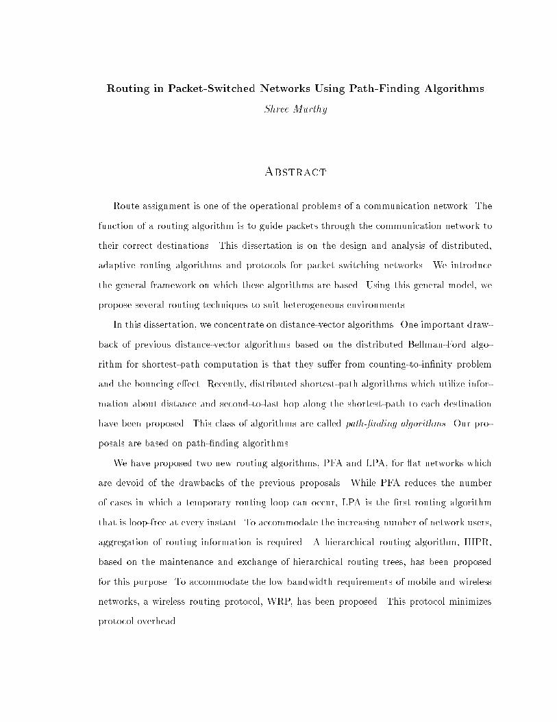
Routing in Packet-Switched Networks Using Path-Finding Algorithms
Shree Murthy
Abstract
Route assignment is one of the operational problems of a communication network. The
function of a routing algorithm is to guide packets through the communication network to
their correct destinations. This dissertation is on the design and analysis of distributed,
adaptive routing algorithms and protocols for packet switching networks. We introduce
the general framework on which these algorithms are based. Using this general model, we
propose several routing techniques to suit heterogeneous environments.
In this dissertation, we concentrate on distance-vector algorithms. One important draw-
back of previous distance-vector algorithms based on the distributed Bellman-Ford algo-
rithm for shortest-path computation is that they su�er from counting-to-in�nity problem
and the bouncing e�ect. Recently, distributed shortest-path algorithms which utilize infor-
mation about distance and second-to-last hop along the shortest-path to each destination
have been proposed. This class of algorithms are called path-�nding algorithms. Our pro-
posals are based on path-�nding algorithms.
We have proposed two new routing algorithms, PFA and LPA, for at networks which
are devoid of the drawbacks of the previous proposals. While PFA reduces the number
of cases in which a temporary routing loop can occur, LPA is the �rst routing algorithm
that is loop-free at every instant. To accommodate the increasing number of network users,
aggregation of routing information is required. A hierarchical routing algorithm, HIPR,
based on the maintenance and exchange of hierarchical routing trees, has been proposed
for this purpose. To accommodate the low bandwidth requirements of mobile and wireless
networks, a wireless routing protocol, WRP, has been proposed. This protocol minimizes
protocol overhead.
To increase the responsiveness of a routing protocol and to guarantee the quality of ser-
vice required by the user, routing and congestion control mechanisms have been integrated.
This protocol ensures that packets arriving into a packet-switched network will be delivered
unless a resource failure prevents it. Using this mechanism, we can ensure certain level of
performance guarantees for network ows.

xii
Acknowledgments
Several people supported me during my graduate study and I would like to thank them
all. First of all, I would like to thank my advisor J.J. Garcia-Luna-Aceves for all his
encouragement, patience and invaluable guidance. He was always there for me whenever I
needed any sort of guidance. I feel very fortunate to have got an opportunity to work with
him and I look forward to work with him in the coming years.
I would like to thank Anujan Varma for being in my proposal committee and for his
valuable comments and suggestions. Many thanks to Patrick Mantey and Darrell Long for
being in my committee and for their valuable suggestions.
Thanks are due to Bill Zaumen for answering all my questions on Drama very patiently
and for making it possible for me to work with Drama for my simulations. Thanks are also
due to Dr. Raphael Rom, for providing support and for bearing with my irregularities in
the work schedule.
Thanks to the coco-group and especially to Jochen and Chane for making working in
the lab so very enjoyable. Thanks to Atul, Hari, Vijay, Pratibha and Jyoti just for being
there. Thanks to Jyoti, Hari and Ewerton for going through my dissertation and for their
suggestions.
Thanks also to Nagesh, Ingrid for their encouragement and to little Kiran.
Most importantly, I would like to thank my parents for all their encouragement, love
and support that has enabled me to live my dreams. Finally, I would like to thank God but
for his grace, nothing would have been possible.
This work was funded in part by the o�ce of Naval Research (ONR) under Grant No. N-
00014-92-J-1807 and by the Defense Advanced Research Projects Agency (DARPA) under
Grant No. DAAB07-95-C-D157.

1
Chapter 1
Introduction
One of the important components of a computer network is the communication subnetwork
which includes the hardware and the software required for the transmission of data within
the network. Traditionally, two di�erent types of networks have supported the communi-
cation needs of end users: the telecom networks (telephone, cable and satellite networks)
and data networks (Internet). The telephone network is designed to support high quality
audio communications. These networks are engineered to provide low delay and �xed band-
width service. Telecom networks are based on circuit-switching mode of operation in which,
at the start of each session, the network determines the connection route and establishes
end-to-end path from sender to receiver. In contrast, data networks are usually based on
packet-switching, where there is no �xed physical path between a sender and a receiver.
Instead, when a sender has a block of data to send, it is received in its entirety and then
forwarded to the next hop along the path to the destination. Even though providing service
guarantees is easier in circuit-switched mode of operation, because of the bursty nature of
the tra�c, packet-switching is favored in the present day Internet. Also, with the increasing
demand for mobile and wireless communication, better techniques need to be developed for
data transfer in a packet-switched environment.
In the context of the internal operation of a network, a connection is usually called
virtual circuit in analogy with the physical circuits setup by the telephone system. The
independent packets of the connectionless organization are called datagrams, in analogy
with data networks. The idea behind a virtual circuit is to avoid having to make routing

2
Table 1.1: Comparison of Datagram and Virtual Circuit Networks
Each packet contains a short VCnumber
Each packet contains the source
Each packet is routedindependently
All VCs passing through thefailed resource are terminated
Resource failure
Suitability
State Information
Congestion control
Connection-oriented and
Routing
Addressing
Route is chosen when VC is setup.All packets follow this route
ISSUE DATAGRAM
State information about each VC
is maintained
and the destination address
Easy if enough buffers can beallocated in advance
Connection-oriented service
Does not hold packet level state
information
VIRTUAL CIRCUIT
Difficult
Packets are lost only duringresource failure
connectionless service
decisions for every packet sent. The route from a source to a destination is chosen as part
of the connection setup mechanism.
In contrast, with a datagram network, no routes are setup in advance. Each packet
is routed independently. Successive packets may follow di�erent routes. While datagram
networks have to do more work, they are more robust and adapt to congestion and fail-
ures easily. Table 1.1 summarizes some of the di�erences between datagrams and virtual
circuits [Tan91].
Routing forms an integral part of the communications subnetwork. The routing algo-
rithm is a part of the network layer which is responsible for deciding on which outbound
queue an incoming packet should be transmitted. It guides packets through the communi-
cation network to their correct destinations. If the network uses datagrams internally, this
decision must be made for every arriving data packet. However, if virtual circuits are used
internally, routing decisions are made only when a new virtual circuit is being set up. The

3
selection of the path towards a destination itself is made by a well-de�ned decision rule
which is referred to as the routing policy.
Regardless of whether routes are chosen independently for each packet or only when new
connections are established, certain properties are desirable in a routing algorithm. Some
of them are:
� Simplicity: Simple algorithms are preferred for ease of implementation and higher
e�ciency in operational networks.
� Robustness with respect to failures and changing conditions: The algorithm must be
able to adjust the routing decisions when tra�c conditions change or when there is
a resource failure. The algorithm monitors the network constantly and updates the
routing information
� Stability of the routing decisions: The routing algorithms should adapt smoothly to
changes in operating conditions. i.e., a small change in operating conditions should
provide a comparatively small change in routing decisions.
� Fairness of the resource allocation: Data ows with the same characteristics should
result in similar packet delay and throughput.
� Optimality of the packet travel times: The routing algorithm should maximize the
network designer's objective function, while satisfying design constraints.
� Loop freedom: At any instant, the paths implied from the routing tables of all hosts
taken together should not have loops. Each router in the path from a source to
destination should be visited only once.
� Convergence characteristics: Time required to converge after a topology change should
not be high. This is required to maintain up-to-date network state information.
� Processing and memory e�ciency: The resources used at each router should be mini-
mal. The computation time spent at a node a�ects the convergence time of the routing
algorithm.
4
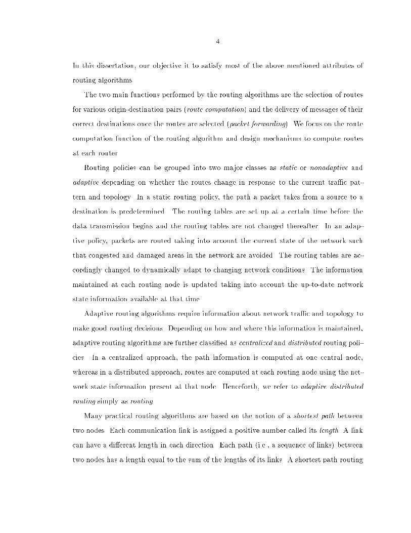
In this dissertation, our objective it to satisfy most of the above mentioned attributes of
routing algorithms.
The two main functions performed by the routing algorithms are the selection of routes
for various origin-destination pairs (route computation) and the delivery of messages of their
correct destinations once the routes are selected (packet forwarding). We focus on the route
computation function of the routing algorithm and design mechanisms to compute routes
at each router.
Routing policies can be grouped into two major classes as static or nonadaptive and
adaptive depending on whether the routes change in response to the current tra�c pat-
tern and topology. In a static routing policy, the path a packet takes from a source to a
destination is predetermined. The routing tables are set up at a certain time before the
data transmission begins and the routing tables are not changed thereafter. In an adap-
tive policy, packets are routed taking into account the current state of the network such
that congested and damaged areas in the network are avoided. The routing tables are ac-
cordingly changed to dynamically adapt to changing network conditions. The information
maintained at each routing node is updated taking into account the up-to-date network
state information available at that time.
Adaptive routing algorithms require information about network tra�c and topology to
make good routing decisions. Depending on how and where this information is maintained,
adaptive routing algorithms are further classi�ed as centralized and distributed routing poli-
cies. In a centralized approach, the path information is computed at one central node,
whereas in a distributed approach, routes are computed at each routing node using the net-
work state information present at that node. Henceforth, we refer to adaptive distributed
routing simply as routing.
Many practical routing algorithms are based on the notion of a shortest path between
two nodes. Each communication link is assigned a positive number called its length. A link
can have a di�erent length in each direction. Each path (i.e., a sequence of links) between
two nodes has a length equal to the sum of the lengths of its links. A shortest path routing

5
algorithm routes each packet along a minimum length (shortest) path between the origin
and destination nodes of the packet. The simplest possibility is for each link to have unit
length (one hop), in which case a shortest path is simply a path with minimum number
of links (hop count). More generally, the length may depend on transmission capacity and
tra�c load. The idea of shortest path algorithms is that the path should contain relatively
few and uncongested links.
Distributed routing algorithms can be subdivided into distance vector algorithms (DVA)
and link-state algorithms (LSA) depending on the method adopted to maintain routing in-
formation in router databases. In a distance vector algorithm, each node has knowledge
of only the local links. The shortest paths are computed using a distributed version of
Bellman-Ford algorithm [BG92] in which nodes exchange their shortest path lengths to
other nodes with their neighbors periodically or on a event-driven basis. Using this infor-
mation received from its neighbors, each node constructs a routing table containing the
distance of the shortest path to every destination in the network. In other words, the pro-
cess of route computation is carried out in a distributed way with each node performing
part of the computation. Examples of distance-vector protocols include the old Arpanet
algorithm [MW77], RIP [Hed88] and Cisco's IGRP [Hed].
In a link-state algorithm, each node has complete information of the network topology
using which each node computes routes independently. When a node detects any change in
the link distances, it sends out an update to all other nodes by broadcasting. Upon receiving
an update, each node recomputes shortest paths to all other nodes using Dijkstra's shortest
path algorithm [BG92] and constructs its new routing table. Some of the link state protocols
are the new Arpanet routing protocol [MRR80], OSPF [Moy94] and ISO's IS-IS [Ora90].
1.1 Problem Formulation
In this dissertation, we concentrate on routing techniques for packet-switched networks using
distance-vector algorithms. These algorithms are applicable to circuit-switched networks
also. In the next few paragraphs we outline the motivation for our work. The main focus of
6
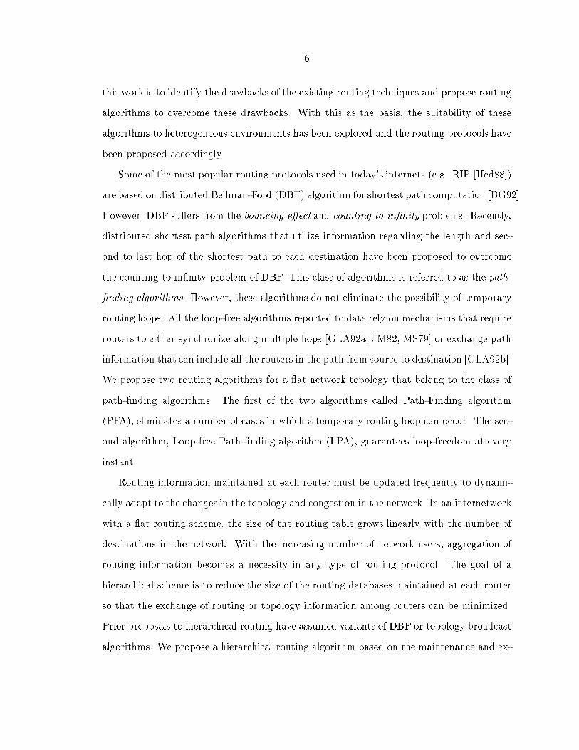
this work is to identify the drawbacks of the existing routing techniques and propose routing
algorithms to overcome these drawbacks. With this as the basis, the suitability of these
algorithms to heterogeneous environments has been explored and the routing protocols have
been proposed accordingly.
Some of the most popular routing protocols used in today's internets (e.g. RIP [Hed88])
are based on distributed Bellman-Ford (DBF) algorithm for shortest path computation [BG92].
However, DBF su�ers from the bouncing-e�ect and counting-to-in�nity problems. Recently,
distributed shortest path algorithms that utilize information regarding the length and sec-
ond to last hop of the shortest path to each destination have been proposed to overcome
the counting-to-in�nity problem of DBF. This class of algorithms is referred to as the path-
�nding algorithms. However, these algorithms do not eliminate the possibility of temporary
routing loops. All the loop-free algorithms reported to date rely on mechanisms that require
routers to either synchronize along multiple hops [GLA92a, JM82, MS79] or exchange path
information that can include all the routers in the path from source to destination [GLA92b].
We propose two routing algorithms for a at network topology that belong to the class of
path-�nding algorithms. The �rst of the two algorithms called Path-Finding algorithm
(PFA), eliminates a number of cases in which a temporary routing loop can occur. The sec-
ond algorithm, Loop-free Path-�nding algorithm (LPA), guarantees loop-freedom at every
instant.
Routing information maintained at each router must be updated frequently to dynami-
cally adapt to the changes in the topology and congestion in the network. In an internetwork
with a at routing scheme, the size of the routing table grows linearly with the number of
destinations in the network. With the increasing number of network users, aggregation of
routing information becomes a necessity in any type of routing protocol. The goal of a
hierarchical scheme is to reduce the size of the routing databases maintained at each router
so that the exchange of routing or topology information among routers can be minimized.
Prior proposals to hierarchical routing have assumed variants of DBF or topology broadcast
algorithms. We propose a hierarchical routing algorithm based on the maintenance and ex-
7
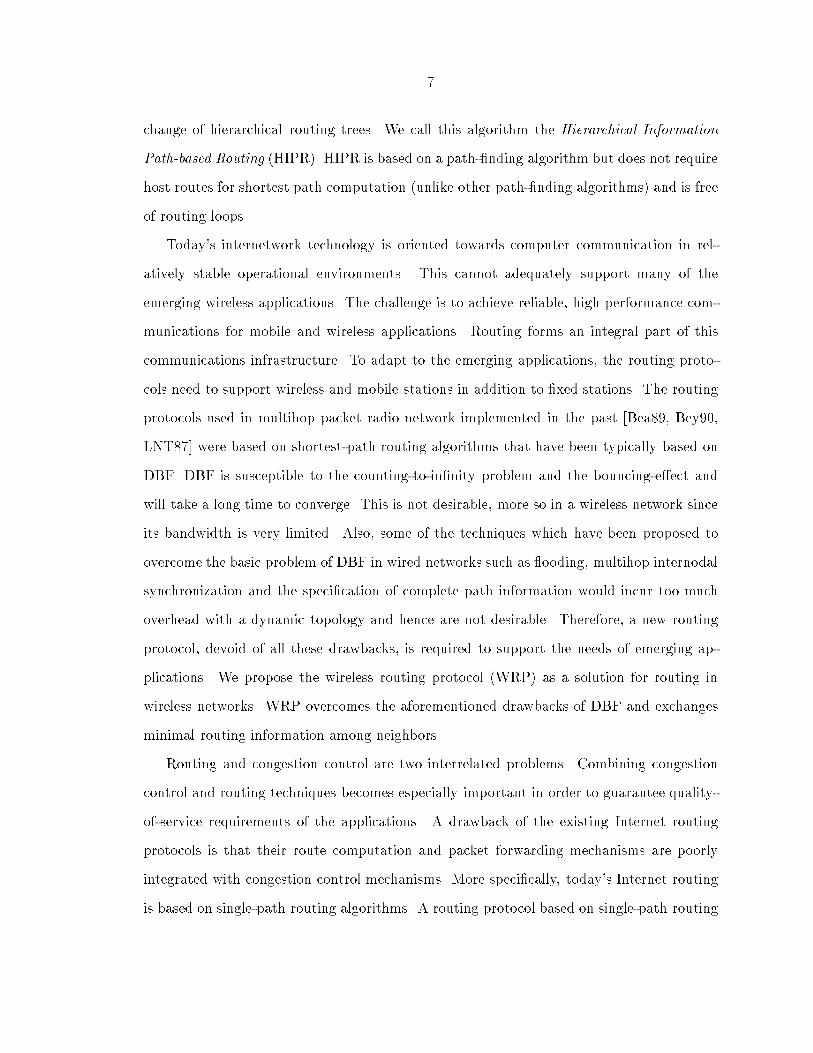
change of hierarchical routing trees. We call this algorithm the Hierarchical Information
Path-based Routing (HIPR). HIPR is based on a path-�nding algorithm but does not require
host routes for shortest path computation (unlike other path-�nding algorithms) and is free
of routing loops.
Today's internetwork technology is oriented towards computer communication in rel-
atively stable operational environments. This cannot adequately support many of the
emerging wireless applications. The challenge is to achieve reliable, high performance com-
munications for mobile and wireless applications. Routing forms an integral part of this
communications infrastructure. To adapt to the emerging applications, the routing proto-
cols need to support wireless and mobile stations in addition to �xed stations. The routing
protocols used in multihop packet radio network implemented in the past [Bea89, Bey90,
LNT87] were based on shortest-path routing algorithms that have been typically based on
DBF. DBF is susceptible to the counting-to-in�nity problem and the bouncing-e�ect and
will take a long time to converge. This is not desirable, more so in a wireless network since
its bandwidth is very limited. Also, some of the techniques which have been proposed to
overcome the basic problem of DBF in wired networks such as ooding, multihop internodal
synchronization and the speci�cation of complete path information would incur too much
overhead with a dynamic topology and hence are not desirable. Therefore, a new routing
protocol, devoid of all these drawbacks, is required to support the needs of emerging ap-
plications. We propose the wireless routing protocol (WRP) as a solution for routing in
wireless networks. WRP overcomes the aforementioned drawbacks of DBF and exchanges
minimal routing information among neighbors.
Routing and congestion control are two interrelated problems. Combining congestion
control and routing techniques becomes especially important in order to guarantee quality-
of-service requirements of the applications. A drawback of the existing Internet routing
protocols is that their route computation and packet forwarding mechanisms are poorly
integrated with congestion control mechanisms. More speci�cally, today's Internet routing
is based on single-path routing algorithms. A routing protocol based on single-path routing

8
is ill-suited to cope with congestion, because the only thing the protocol can do to react
to congestion is to change the route used to reach a destination, and this could lead to
unstable oscillatory behavior [Ber82]. In many networks there are several paths between
pairs of nodes that are almost equally good. Better performance can be achieved by split-
ting the tra�c over several paths to reduce the load on each of the links. This technique
of using multiple routes between a single pair of nodes is called multipath routing. This is
similar to inverse multiplexing in circuit-switched networks where the primary motivation
is to provide high bandwidth with the limitation of low bandwidth links. Furthermore, in
a datagram network, routers forward packets only on a best-e�ort basis and drop the pack-
ets when congestion occurs. The routers adapt to congestion only after network resources
have already been wasted. We propose a new framework for dynamic multipath routing in
packet-switched networks that attempts to prevent the over-utilization of network resources
and hence avoid congestion. This protocol illustrates the provision of performance guaran-
tees in a connectionless routing architecture. Using this approach, we propose a two-tier
architecture in which the end users can request performance guarantees similar to a connec-
tion oriented architecture and, within the network, packet transmission is done hop-by-hop
as in a connection-less network.
1.2 Dissertation Overview
This dissertation is organized as follows:
Chapter 2 gives an overview of the routing algorithms that are being used in today's
internetwork. We highlight the problems in the existing algorithms and explain the
working of the basic path-�nding algorithm. We also introduce the network model
and some of the terminologies used in the dissertation.
Chapter 3 presents two path-�nding algorithms, PFA and LPA, which eliminate the loop-
ing problem of the existing distance-vector routing algorithms. We show through sim-

9
ulations that these two algorithms have better performance than the state of the art
routing algorithms such as DUAL and an ideal link-state algorithm.
Chapter 4 proposes a novel methodology for routing in hierarchical networks. We formally
verify the hierarchical routing algorithm and present some simulation results. The
performance of this algorithm is compared with that of OSPF.
Chapter 5 describes a wireless routing protocol which is suitable in a packet-radio net-
work. Simulation results of the basic routing algorithm are presented to evaluate the
performance of the proposed protocol. Some implementation issues are also discussed.
Chapter 6 proposes a novel approach for integrating routing with congestion control. A
worst-case delay bound for this dynamic solution is derived. A two-tier architecture
is also proposed for mapping connection-oriented ows to connection-less ows and
thereby guaranteeing certain level of QoS to end users of a packet-switched network.
Chapter 7 gives a summary of this work, together with some conclusions and directions
for future research.
10
Chapter 2
Background
As explained in the previous chapter, routing algorithms are responsible for forwarding the
data packets over routes to provide good or optimal performance. Consequently, a routing
protocol is required to maintain the status of all the routes in the network. A router
runs a speci�ed routing algorithm to compute routes to all known destinations. A routing
algorithm mainly consists of two parts { an initialization step and a recurring step that is
repeated until the algorithm terminates. The recurring step involves updating the minimum
distance of each router for all destinations until the algorithm converges to correct shortest
path distances. The routing algorithms di�er in the way by which the updating step is
implemented. There are two types of adaptive routing algorithms { link state and distance
vector algorithms.
Link-state Algorithms: In the link-state approach, each router maintains a complete
view of the network topology and the cost associated with each link [MRR78, MRR80].
The topology information is updated regularly. A router broadcasts regularly the link state
information of all its outgoing links to all other routers by ooding. A complete computation
of the best routes is done at each node using the information present in its local topology
database. When a router receives information about the change in the link cost, it updates
its view of the network and applies a shortest path algorithm to choose its next hop to each
destination.
Link state algorithms are basically free of long-term loops. Routers may not always
have a consistent view of the network topology, because of the time updates take to reach
11
all routers. This inconsistent view of the network can lead to the formation of loops, which
are temporary and disappear in the time it takes for all routers to have the same topological
information.
Link state algorithms have a disadvantage of not being scalable in terms of number of
messages exchanged and the memory required to maintain the state of the entire network
topology. Each time the topology changes, all network nodes have to recompute their
routing tables, which creates a peak of activity.
Shortest Path First (SPF) [McQ74] is a link-state protocol in which each node computes
and broadcasts the costs of its outgoing links periodically and applies Dijkstra's shortest
path algorithm [BG92] to determine the next hop; other routing protocols that work on the
same link-state approach are IS-IS [Ora90, Per91], and OSPF [Moy94].
Distance-Vector Algorithms: Distance-vector algorithms are often referred to as Bellman-
Ford algorithms because they are based on the shortest-path computation algorithm by R.E.
Bellman [Bel57]. Distance-vector algorithms have been used in several packet-switched net-
works such as Arpanet.
In a distance-vector algorithm, a router knows the length of the shortest-path (distance)
from each of its neighbors to every destination in the network and uses this information to
compute its own distance and the next router (successor) to each destination. Well-known
examples of routing protocols which are based on distance-vector algorithms (DVA), are the
routing information protocol (RIP) [Hed88], the HELLO protocol [Mil83a], the gateway-to-
gateway protocol (GGP) [HS82], the exterior gateway protocol (EGP) [Mil83b] and the old
Arpanet routing protocol [McQ74]. All these DVAs have used variants of the distributed
Bellman-Ford algorithm (DBF) for shortest-path computation [BG92].
Distance-vector algorithms perform their route computation on a per-destination basis.
If a link fails, only routes for those destinations which were routed over the failed link need
to be recomputed. Moreover, the computation is localized to one part of the network only
{ the routers upstream of the failed link. Therefore, distance-vector algorithms are simpler.

12
The primary disadvantages of DBF are routing-table loops and counting-to-in�nity prob-
lem [GLA]. A routing-table loop is a path speci�ed in the routers' routing tables at a
particular point in time, such that the path visits the same router more than once before
reaching the intended destination. A router is said to be counting-to-in�nity when it incre-
ments its distance to a destination until it reaches a prede�ned maximum distance value.
Some solutions such as split horizon and poisson reverse have been proposed to overcome
these basic problems [Hui95].
2.1 Network Model
A computer network G is modeled as an undirected graph represented as G(V;E), where
V is the set of nodes and E is the set of edges or links connecting nodes. Each node
represents a router and is a computing unit involving a processor, local memory, and input
and output queues with unlimited capacity. Extending the model to account for end node
(link) destinations attached to routers is trivial. A functional bidirectional link connecting
nodes i and j is denoted by (i; j) and is assigned a positive weight in each direction. A link
is assumed to exist in both directions at the same time. All messages received (transmitted)
by a node are put in the input (output) queue on a �rst-come-�rst-serve (FCFS) basis and
are processed in that order. An underlying protocol assures that:
� Every node knows who its neighbors are; this implies that a node within a �nite time
detects the existence of a new neighbor or the loss of connectivity with a neighbor, or
the change in the cost of an adjacent link.
� All packets transmitted over an operational link are received correctly and in the
proper sequence within a �nite time. (This assumption is made for convenience.
Reliable message transmission can be easily incorporated into the routing protocol
(e.g. [MGLA95, Moy94])
� All update messages, changes in the link-cost, link failures and link recoveries are
processed one at a time in the order in which they occur.

13
Each node is given a unique identi�er. Any link cost can vary over time but is always
positive. The distance between the two nodes in the network is measured as the sum of the
link costs of the shortest path between nodes.
When a link fails, the corresponding distance entry in a node's distance and routing
tables are marked as in�nity. A node failure is modeled as all links incident on that node
failing at the same time. A change in the operational status of a link or a node is assumed
to be noti�ed to its neighboring nodes within a �nite time. These services are assumed to
be reliable and are provided by the lower level protocols.
Routing updates which are sent by a router to all its neighboring nodes can be of two
types { periodic (time driven) and triggered (event driven). Periodic routing updates are sent
periodically when the periodic update timer expires. The value of this timer depends on the
network propagation delay and latency. Triggered updates increases the responsiveness of
the protocol by requesting routers to send updates as soon as certain event occurs. Typical
events are the changing of a local metric value, or the reception of a routing table update
from a neighbor. This procedure speeds up the convergence time of the routing algorithm.
The algorithms we propose use event-driven updating mechanism.
2.2 Notations and De�nitions
A path from node i to node j is a sequence of nodes where (i; n1), (nx; nx+1), (nr; j) are
links in the path. A simple path from i to j is a sequence of nodes in which no node is
visited more than once. A implicit path from i to j is a path that is derived from predecessor
node information. The paths between any pair of nodes and their corresponding distances
change over time in a dynamic network. At any point in time, node i is connected to node
j if a path exists from i to j at that time. The network is said to be connected if every pair
of operational nodes are connected at a given time.
14
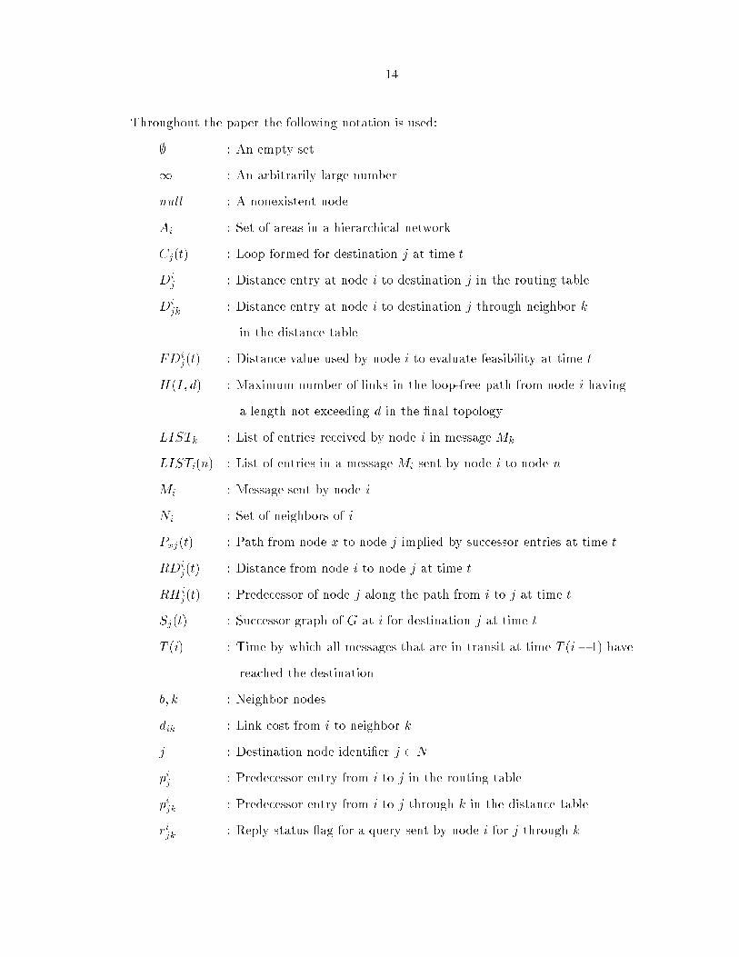
Throughout the paper the following notation is used:
; : An empty set.
1 : An arbitrarily large number.
null : A nonexistent node.
Ai : Set of areas in a hierarchical network
Cj(t) : Loop formed for destination j at time t
Dij : Distance entry at node i to destination j in the routing table
Dijk : Distance entry at node i to destination j through neighbor k
in the distance table
FDij(t) : Distance value used by node i to evaluate feasibility at time t
H(I; d) : Maximum number of links in the loop-free path from node i having
a length not exceeding d in the �nal topology
LISTk : List of entries received by node i in message Mk.
LISTi(n) : List of entries in a message Mi sent by node i to node n.
Mi : Message sent by node i.
Ni : Set of neighbors of i
Pxj(t) : Path from node x to node j implied by successor entries at time t
RDij(t) : Distance from node i to node j at time t
RH ij(t) : Predecessor of node j along the path from i to j at time t
Sj(t) : Successor graph of G at i for destination j at time t
T (i) : Time by which all messages that are in transit at time T (i� 1) have
reached the destination
b; k : Neighbor nodes
dik : Link cost from i to neighbor k
j : Destination node identi�er j 2 N
pij : Predecessor entry from i to j in the routing table
pijk : Predecessor entry from i to j through k in the distance table
rijk : Reply status ag for a query sent by node i for j through k

15
sij : Successor from node i to j
tagij(t) : Tag at node i for destination j at time t
uij(t) : Update ag
The time at which the value of a variable applies is speci�ed only when it is necessary.
The successor to destination j for any node is simply referred to as the successor of that
node, and the same reference applies to other information maintained by a node. Similarly,
updates, queries and responses refer to destination j, unless stated otherwise.
In the algorithm's description, the time at which the value of a variable X of the algo-
rithm applies is speci�ed only when it is necessary; the value of X at time t is denoted by
X(t).
2.3 Evolution of Distance-Vector Algorithms
One of the earliest implementations of DVA was the routing protocol implemented in the
Arpanet in the early 1970s. In this protocol, every router in the networkmaintains a distance
and a routing table. The shortest path information for all destinations is maintained in the
routing table. A router examines its routing table entries to determine the shortest path to
a particular destination before sending a packet to that destination.
Many approaches have been proposed in the past to solve, at least in part, the looping
problems in DVAs. A widely known proposal is the split-horizon technique, which avoids
ping-pong looping, whereby two nodes choose each other as the successor to a destination
[Ceg75, Sch86]. Another well known technique which has been proposed is the use of
hold downs. Both of these approaches do not completely solve the counting-to-in�nity
problem [GLA]. Some other solutions have also been proposed to overcome this problem
[GLA].
Figure 2.1 illustrates the looping and bouncing e�ect scenarios. Consider a three-node
network with n1 being the destination node. Assume initially all nodes maintain correct
routing table entries. Nodes n2 and n3 choose nodes n1 and n2 as their successors respec-

16
n31
n1
n2
1100
Figure 2.1: Counting-to-In�nity Problem
tively. Now, if link (n1; n2) fails, based on the distance table entries, node n2 will choose
n3 as its successor to destination n1. This information is sent to n3 (i.e., n2 announces a
distance of 3 to reach n1), which leads to the formation of a routing loop between nodes
n2 and n3. Furthermore, since the distances of n2 and n3 are much less than 100, which
is the cost of the link (n1; n3), nodes n2 and n3 will keep increasing their distances till a
distance value > 100 is reached. After this, the distance converges and the correct path
is chosen. Thus, we can see that, using DBF, nodes have to go through a long period of
message exchanges among nodes belonging to loops before the algorithm converges. This
is referred to as the counting-to-in�nity problem.
Some of the most popular routing protocols used in today's Internet (e.g., RIP [Hed88])
are based on the distributed Bellman-Ford algorithm (DBF) for shortest-path computa-
tion [BG92]. The counting-to-in�nity problem is overcome in one of the three ways in
existing Internet routing protocols. OSPF [Moy94] relies on broadcasting complete topol-
ogy information among routers, and organizes the Internet hierarchically to cope with the
overhead incurred with topology broadcast. BGP [RL94] exchanges distance vectors that
specify complete paths to destinations. EIGRP [Far93] uses a loop-free routing algorithm
called DUAL [GLA92a], which is based on internodal coordination that can span multiple
hops; DUAL also eliminates temporary routing loops.
Recently, distributed shortest-path algorithms [CRKGLA89, Hag83, Hum91, RF91,
Mur94] that utilize information regarding the length and second-to-last hop (predecessor

17
Dest
Routing
Table of n1
n1
n2
n3
n4
n5
n6
n7
3, n6, n5
4, n6, n2
6, n6, n7
2, n6, n6
1, n6, n1
5, n6 n3
0, *, *
(d)
Dest
Routing
Table of n1
n1
n2
n3
n4
n5
n6
n7
3, n6, n5
4, n6, n2
6, n6, n7
2, n6, n6
1, n6, n1
5, n6 n3
0, *, *
Dest
Routing
Table of n1
n1
n2
n3
n4
n5
n6
n7
3, n6, n5
4, n6, n2
6, n6, n7
2, n6, n6
1, n6, n1
5, n6 n3
0, *, *
Dest
Routing
Table of n1
n1
n2
n3
n4
n5
n6
n7
3, n6, n5
4, n6, n2
6, n6, n7
2, n6, n6
1, n6, n1
5, n6 n3
0, *, *
(a) (b) (c)
Figure 2.2: Path Traversal using Predecessor Information
or node next to the last hop) of the shortest path to each destination have been proposed
(path-�nding algorithms) to eliminate the counting-to-in�nity problem of DBF.
2.4 Path-Finding Algorithms
Path-�nding algorithms eliminate the counting-to-in�nity problem of DBF using predecessor
information. Predecessor information can be used to infer an implicit path to a destination.
Using this path information, routing loops can be detected. Each distance entry in the
distance and routing tables is associated with the predecessor node information. The design
of the path-�nding algorithm is such that at all times, the distance and routing table entries
satisfy the following property:
The path implicit in a distance entry from router i to destination j through a
neighbor k, Dkij, with associated predecessor h
kij = h, is the path implicit to node
h, Dkih, augmented by link (h; j).
If each column in the distance and routing tables of a router satis�es this property at all
times, then it can be used to maintain only simple paths to destinations.
Figure 2.2 illustrates the path traversal using predecessor information. Let n1{n7 be
the nodes in a network. The �gure shows the routing table entries at node n1. A routing
table is a vector with each entry specifying the destination j, current shortest distance Dij ,
successor sij and the predecessor pij . In�nite distance is represented as1 and null path by *.

18
Suppose node n1 want to determine if its neighbor n7 is in the shortest path to destination
n2. Node n1 starts the trace from the entry for destination n2 (Figure 2.2(a)) and �nds
that the predecessor to n2 is node n5. Subsequently, n1 walks through the predecessors of
its path to n5 and n6 until it reaches node n1 itself (Figure 2.2(d)). From this, node n1
determines n7 is not in the path from n1 to n2 (not encountered during the trace). The
sequence of predecessors encountered during such a trace represents a path from n1 to n2.
This is referred to as the implicit path or the path extracted from the predecessor node
information [CRKGLA89].
Although path-�nding algorithms provide a marked improvement over DBF, the exist-
ing path-�nding algorithms [CRKGLA89, GLA86, Hag83, Hum91, RF91] do not eliminate
the possibility of temporary loops. The algorithms we have proposed are similar to previ-
ous path-�nding algorithms with respect to maintaining predecessor information in distance
and routing tables. Because each router reports to its neighbors the predecessor to each
destination, any router can traverse the path speci�ed by the predecessors from any desti-
nation back to a neighbor router to determine if using that neighbor as its successor would
create a path that contains a loop (i.e., involves the router itself). Furthermore, a router
detects a temporary loop within a �nite time that depends on the speed with which correct
predecessor information reaches the router, and not on the distance values of the paths
o�ered by its neighbors; therefore, temporary loops are detected much faster than in DBF
and its variations.
The next chapter describes the two algorithms, path-�nding algorithm (PFA) and loop-
free path-�nding algorithm (LPA) and present some of their performance results. This
forms the basis of our discussion in this dissertation.

19
Chapter 3
New Path-Finding Algorithms
This chapter describes two routing algorithms which we propose for a at network. The
two algorithms, path-�nding algorithm (PFA) and loop-free path-�nding algorithm (LPA),
belong to the class of path-�nding algorithms which forms the basis of our discussion in the
rest of the dissertation. The working of the basic path-�nding algorithm has been explained
in the previous chapter.
3.1 Path-Finding Algorithm
PFA uses predecessor information to extract implicit paths from its distance and routing
tables without excessive overhead. It substantially reduces the number of cases in which
routing loops can occur. Each node maintains the shortest-path spanning tree reported
by its neighbors, and uses this information and the information regarding the cost of the
adjacent links to generate its own shortest-path spanning trees. The fact that PFA reduces
temporary looping accounts for its superior performance over DUAL and the ideal link
state algorithm (ILS). In addition to this, PFA also has an e�cient updating mechanism.
Each time an update is received by a router, the distance table and routing table entries
are updated to re ect the change in the network state and thus maintain correct path
information to all destinations.

20
3.1.1 PFA Description
Each node maintains a distance table, a routing table and a link-cost table. The distance
table at node i is a matrix containing the distance (Dijk) and predecessor (pijk) entries
(path information) for all destinations (j) through all its neighbors (k). The routing table
is a column vector of minimum distance to each destination (dij) and its corresponding
predecessor (pij) and successor (sij) information. The link-cost table lists the cost of each
link adjacent to the node (lik); the cost of a failed link is considered to be in�nity. An
update message contains the source and the destination node identi�ers, and the distance
and predecessor for one or more destinations.
When a node i receives an update message from its neighbor k regarding destination
j, the distance and the predecessor entries in the distance table are updated (Step 1). A
unique feature of PFA is that node i also determines if the path to destination j through
any of its other neighbors fb 2 Nijb 6= kg includes node k. If the path implied by the
predecessor information reported by node b includes node k, then the distance entry of that
path is also updated as Dijb = Di
kb +Dkj and the predecessor is updated as pijb = pkj . Thus,
a node can determine whether or not an update received from k a�ects its other distance
and routing table entries. Before updating the routing table, node i checks for all simple
paths to j reported by its neighbors, and the shortest of these simple paths becomes the
path from i to j. This implies that at each stage node i checks for the simple paths and
avoids loops. Link or node failures, recoveries and link-cost changes are handled similarly.
In contrast to PFA, which makes a node i check the consistency of predecessor informa-
tion reported by all its neighbors each time it processes an event involving a neighbor k,
all previous path-�nding algorithms [CRKGLA89, Hum91, RF91] check the consistency of
the predecessor only for the neighbor associated with the input event. This unique feature
of PFA accounts for its fast convergence after a single resource failure or recovery as it
eliminates more temporary looping situations than previous path-�nding algorithms.
The following example illustrates the working of the algorithm. Consider a four node
network shown in Figure 3.1(a). Let PFA be used at each node in this network. All links

21
(10,i)
(b)
(c) (d)
(a)
1
1
1
10
510
(infinity,-)
(infinity,-)
j
bi
k k
b i
k
bi
j
j
ij
k
b
(0,j)
(2,k)
(1,k)
(2,k)
(10,i)
(0,j)
(10,b)
(0,j)
(2,k)(2,k)
(0,j)
(11,b)
Figure 3.1: Example of PFA's Operation
and nodes are assumed to have the same propagation delay. Link-costs are as indicated in
the �gure and are assumed to be the same in both the directions. Node i is the source, j
is the destination and nodes k and b are the neighbors of node i. The directed lines next
to links indicate the direction of update messages and the label in parentheses gives the
distance and the predecessor to destination j. This �gure focuses on update messages to
destination j only.
When link (j; k) fails, nodes j and k send update messages to their neighboring nodes
as shown in Figure 3.1(b). In this example, node k is forced to report an in�nite distance
to j as nodes b and i have reported node k as part of their path to destination j. Node
b processes node k's update and selects link (b; j) to destination j. This is because of
the e�cient updating mechanism of PFA that forces node b to purge any path to node
j involving node k. Also, when i gets node k's update message, i updates its distance
table entry through neighbor k and checks for the possible paths to destination j through
any other neighboring nodes. Thus, a node examines the available paths through its other
neighboring nodes and updates the distance and the routing table entries accordingly. This
results in the selection of the link (i; j) to the destination j (Figure 3.1(c)). When node i
receives b's update reporting an in�nite distance, node i does not need to update its routing

22
LOS-NETTOS NSFNET-T1
ARPANET
Figure 3.2: Simulated Topologies
table as it already has correct path information (Figure 3.1(d)). Similarly, updates sent by
node k reporting a distance of 11 to destination j will not a�ect the path information of
nodes i and b. This illustrates how the e�cient updating mechanism of PFA helps in the
reduction of the formation of temporary routing loops in the explicit paths.
The proofs of correctness, convergence and complexity of PFA are given elsewhere [Mur94].
The worst-case complexity of PFA has been found to be O(h) for single recovery/failure, h
being the height of the tree.
3.1.2 Simulation Environment
The performance of the proposed routing algorithms is evaluated by simulations. The
simulation results of these algorithms have been compared with that of DUAL and an ideal
link-state algorithm (ILS), which uses Dijkstra's shortest path algorithm for shortest path
computation.
The di�using update algorithm (DUAL) proposed by J.J. Garcia-Luna-Aceves aims at
removing transient temporary loops. DUAL is based on the di�using algorithm for partial
route updates proposed by E.W. Dijkstra and C.S. Scholten in 1980 [DS80] and on the
remark that one cannot create a loop by picking a shorter path to the destination [Jaf88].
23
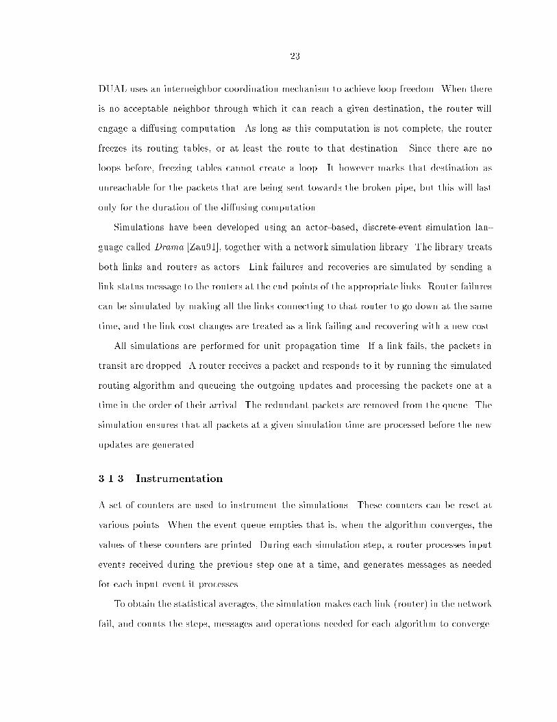
DUAL uses an interneighbor coordination mechanism to achieve loop freedom. When there
is no acceptable neighbor through which it can reach a given destination, the router will
engage a di�using computation. As long as this computation is not complete, the router
freezes its routing tables, or at least the route to that destination. Since there are no
loops before, freezing tables cannot create a loop. It however marks that destination as
unreachable for the packets that are being sent towards the broken pipe, but this will last
only for the duration of the di�using computation.
Simulations have been developed using an actor-based, discrete-event simulation lan-
guage called Drama [Zau91], together with a network simulation library. The library treats
both links and routers as actors. Link failures and recoveries are simulated by sending a
link status message to the routers at the end points of the appropriate links. Router failures
can be simulated by making all the links connecting to that router to go down at the same
time, and the link cost changes are treated as a link failing and recovering with a new cost.
All simulations are performed for unit propagation time. If a link fails, the packets in
transit are dropped. A router receives a packet and responds to it by running the simulated
routing algorithm and queueing the outgoing updates and processing the packets one at a
time in the order of their arrival. The redundant packets are removed from the queue. The
simulation ensures that all packets at a given simulation time are processed before the new
updates are generated.
3.1.3 Instrumentation
A set of counters are used to instrument the simulations. These counters can be reset at
various points. When the event queue empties that is, when the algorithm converges, the
values of these counters are printed. During each simulation step, a router processes input
events received during the previous step one at a time, and generates messages as needed
for each input event it processes.
To obtain the statistical averages, the simulation makes each link (router) in the network
fail, and counts the steps, messages and operations needed for each algorithm to converge.

24
It then makes the same link (router) recover and repeats the process. The average is then
taken over all link (router) failures and recoveries. The routing algorithm was allowed to
converge after each such change. In all cases, routers were assumed to perform computations
in zero time and links were assumed to provide one time unit of delay. For the failure and
recovery runs, the costs are set to unity. Both the mean and the standard deviation are
computed for each counter; the four counters used are
� Update Count: The total number of updates (including queries and replies where
applicable) and changes in link status processed by routers.
� Message Count: The total number of packets transmitted over the network. Each
packet may contain multiple updates.
� Duration: The total elapsed time it takes for an algorithm to converge.
� Operations: The total number of operations performed by all nodes in the network.
The operation count is incremented whenever an event occurs, but also counts the
number of times the statement within a for or (while) loop are executed.
There is no sampling error for the results because all possible cases are covered in the
simulations. Both the mean and the standard deviation of the distributions are given.
3.1.4 Simulation Results
The performance of PFA has been compared with DBF, DUAL and ILS. The simulations
were run on several network topologies such as Los-Nettos, Nsfnet and Arpanet (Figure 3.2).
We choose these topologies to compare the performance of routing algorithms for well-known
cases, given that we cannot sample a large enough number of networks to make statistically
justi�able statements about how an algorithm scales with network parameters. Here we
present the simulation results of Arpanet topology only.
For the routing algorithms under consideration, there is only one shortest path between a
source and a destination pair and we do not consider null paths from a router to itself. Data
was collected for a large number of topology changes to determine statistical distributions.

25
10
100
1000
10000
0 10 20 30 40 50 60 70
ME
SS
AG
ES
LINK FAILURES
PFADBF
DUALILS
0
10
20
30
40
50
60
0 10 20 30 40 50 60 70
ST
EP
S
LINK FAILURES
PFADBF
DUALILS
Figure 3.3: ARPANET Link Failure
0
50
100
150
200
250
300
350
0 10 20 30 40 50 60 70
ME
SS
AG
ES
LINK RECOVERIES
PFADBF
DUALILS
0
5
10
15
20
0 10 20 30 40 50 60 70
ST
EP
S
LINK RECOVERIES
PFADBF
DUALILS
Figure 3.4: ARPANET Link Recovery
Total Response to a Single Resource Change
The graphs in Figures 3.3 and 3.4 depicts the number of messages exchanged and the number
of steps required before each algorithm converges for every link failing and recovering in
the Arpanet topology. Similar graphs for every router failing and recovering is given in
Figures 3.5 and 3.6 respectively. All topology changes are performed one at a time and the
algorithms were allowed to converge after each such change before the next resource change
occurs. The ordinates of the graphs represents the identi�ers of the links and the nodes
while the data points show the number of messages exchanged after each resource change
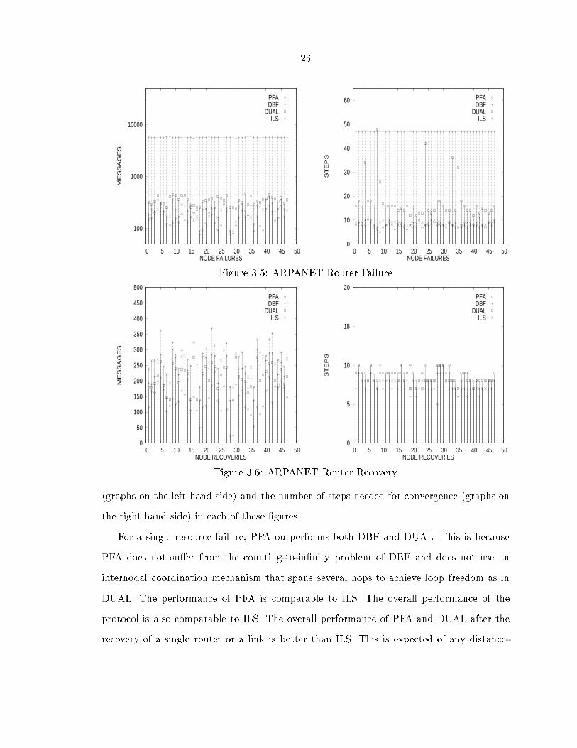
26
100
1000
10000
0 5 10 15 20 25 30 35 40 45 50
ME
SS
AG
ES
NODE FAILURES
PFADBF
DUALILS
0
10
20
30
40
50
60
0 5 10 15 20 25 30 35 40 45 50
ST
EP
S
NODE FAILURES
PFADBF
DUALILS
Figure 3.5: ARPANET Router Failure
0
50
100
150
200
250
300
350
400
450
500
0 5 10 15 20 25 30 35 40 45 50
ME
SS
AG
ES
NODE RECOVERIES
PFADBF
DUALILS
0
5
10
15
20
0 5 10 15 20 25 30 35 40 45 50
ST
EP
S
NODE RECOVERIES
PFADBF
DUALILS
Figure 3.6: ARPANET Router Recovery
(graphs on the left hand side) and the number of steps needed for convergence (graphs on
the right hand side) in each of these �gures.
For a single resource failure, PFA outperforms both DBF and DUAL. This is because
PFA does not su�er from the counting-to-in�nity problem of DBF and does not use an
internodal coordination mechanism that spans several hops to achieve loop freedom as in
DUAL. The performance of PFA is comparable to ILS. The overall performance of the
protocol is also comparable to ILS. The overall performance of PFA and DUAL after the
recovery of a single router or a link is better than ILS. This is expected of any distance-
27
vector algorithm. The convergence time of PFA and DUAL is also comparable to that of
ILS. For a single resource recovery also PFA and DUAL are superior to ILS.
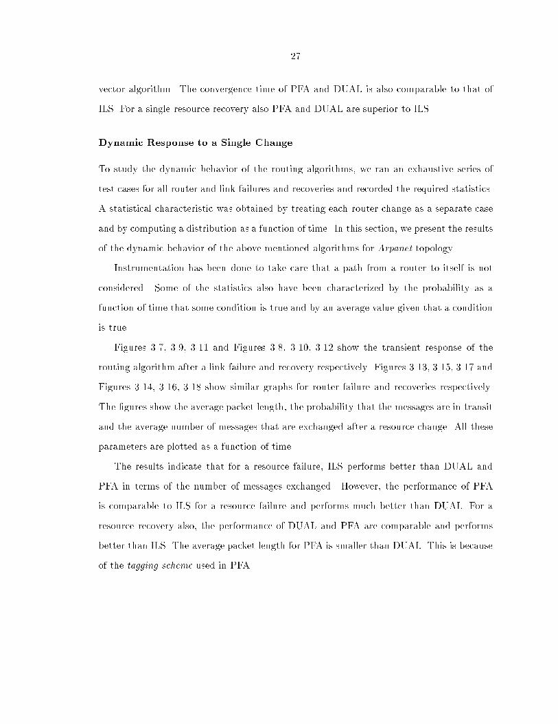
Dynamic Response to a Single Change
To study the dynamic behavior of the routing algorithms, we ran an exhaustive series of
test cases for all router and link failures and recoveries and recorded the required statistics.
A statistical characteristic was obtained by treating each router change as a separate case
and by computing a distribution as a function of time. In this section, we present the results
of the dynamic behavior of the above mentioned algorithms for Arpanet topology.
Instrumentation has been done to take care that a path from a router to itself is not
considered. Some of the statistics also have been characterized by the probability as a
function of time that some condition is true and by an average value given that a condition
is true.
Figures 3.7, 3.9, 3.11 and Figures 3.8, 3.10, 3.12 show the transient response of the
routing algorithm after a link failure and recovery respectively. Figures 3.13, 3.15, 3.17 and
Figures 3.14, 3.16, 3.18 show similar graphs for router failure and recoveries respectively.
The �gures show the average packet length, the probability that the messages are in transit
and the average number of messages that are exchanged after a resource change. All these
parameters are plotted as a function of time.
The results indicate that for a resource failure, ILS performs better than DUAL and
PFA in terms of the number of messages exchanged. However, the performance of PFA
is comparable to ILS for a resource failure and performs much better than DUAL. For a
resource recovery also, the performance of DUAL and PFA are comparable and performs
better than ILS. The average packet length for PFA is smaller than DUAL. This is because
of the tagging scheme used in PFA.

28
0.0
2.0
4.0
6.0
8.0
10.0
12.0
5 10 15 20 25
AV
ER
AG
E P
AC
KE
T L
EN
GT
H
TIME AFTER LINK FAILURE
PFADUAL
ILS
Figure 3.7: Avg pkt len for Link Fail-ure
0.0
2.0
4.0
6.0
8.0
10.0
12.0
14.0
2 4 6 8 10 12 14
AV
ER
AG
E P
AC
KE
T L
EN
GT
H
TIME AFTER LINK RECOVERY
PFADUAL
ILS
Figure 3.8: Avg pkt len for Link Re-covery
0.0
0.2
0.4
0.6
0.8
1.0
5 10 15 20 25
PR
OB
AB
ILIT
Y
TIME AFTER LINK FAILURE
PFADUAL
ILS
Figure 3.9: Prob of pkts for LinkFailure
0.0
0.2
0.4
0.6
0.8
1.0
2 4 6 8 10 12 14
PR
OB
AB
ILIT
Y
TIME AFTER LINK RECOVERY
PFADUAL
ILS
Figure 3.10: Prob of pkts for LinkRecovery
0.0
5.0
10.0
15.0
20.0
25.0
30.0
35.0
5 10 15 20 25
AV
ER
AG
E N
UM
BE
R O
F P
AC
KE
TS
TIME AFTER LINK FAILURE
PFADUAL
ILS
Figure 3.11: Avg num of pkts forLink Failure
0.0
5.0
10.0
15.0
20.0
25.0
30.0
35.0
2 4 6 8 10 12 14
AV
ER
AG
E N
UM
BE
R O
F P
AC
KE
TS
TIME AFTER LINK RECOVERY
PFADUAL
ILS
Figure 3.12: Avg num of pkts forLink Recovery

29
0.0
2.0
4.0
6.0
8.0
10.0
12.0
0 5 10 15 20 25 30 35 40 45 50
AV
ER
AG
E P
AC
KE
T L
EN
GT
H
TIME AFTER NODE FAILURE
PFADUAL
ILS
Figure 3.13: Avg pkt len for RouterFailure
0.0
10.0
20.0
30.0
40.0
50.0
60.0
70.0
0 5 10 15 20
AV
ER
AG
E P
AC
KE
T L
EN
GT
H
TIME AFTER NODE RECOVERY
PFADUAL
ILS
Figure 3.14: Avg pkt len for RouterRecovery
0.0
0.2
0.4
0.6
0.8
1.0
0 5 10 15 20 25 30 35 40 45 50
PR
OB
AB
ILIT
Y
TIME AFTER NODE FAILURE
PFADUAL
ILS
Figure 3.15: Prob of pkts for RouterFailure
0.0
0.2
0.4
0.6
0.8
1.0
0 5 10 15 20
PR
OB
AB
ILIT
Y
TIME AFTER NODE RECOVERY
PFADUAL
ILS
Figure 3.16: Prob of pkts for RouterRecovery
0.0
10.0
20.0
30.0
40.0
50.0
60.0
0 5 10 15 20 25 30 35 40 45 50
AV
ER
AG
E N
UM
BE
R O
F P
AC
KE
TS
TIME AFTER NODE FAILURE
PFADUAL
ILS
Figure 3.17: Avg num of pkts forRouter Failure
0.0
10.0
20.0
30.0
40.0
50.0
60.0
70.0
0 5 10 15 20
AV
ER
AG
E N
UM
BE
R O
F P
AC
KE
TS
TIME AFTER NODE RECOVERY
PFADUAL
ILS
Figure 3.18: Avg num of pkts forRouter Recovery

30
1.0
10.0
100.0
1 10 100 1000 10000AV
E N
UM
OF
MS
GS
WH
EN
MS
GS
AR
E IN
TR
AN
SIT
INTERARRIVAL TIME
PFADUAL
ILS
Figure 3.19: Average Number of Messages
0.1
1.0
10.0
100.0
1 10 100 1000 10000
AV
ER
AG
E M
ES
SA
GE
LE
NG
TH
INTERARRIVAL TIME
PFADUAL
ILS
Figure 3.20: Average Message Length
Response to Multiple Link-Cost Changes
The steady-state behavior of the algorithms is more interesting with multiple link-cost
changes than the transient response after each topology change. Figures 3.19 and 3.20
shows the average number of update messages when messages are in transit and the average
length of messages as a function of the interarrival times between link-cost changes for PFA,
DUAL and ILS respectively. This again is for Arpanet topology. From [ZGLA92], it has
been observed that the behavior of DUAL and ILS for multiple link-cost changes is similar
for di�erent network topologies; our conjecture is that the same is true for PFA also.
For very long interarrival times, the number of messages during busy periods is inde-
pendent of the interarrival time because the probability of two topology changes occurring
simultaneously is small. In this case, the performance approaches that of single link-cost
change. When the interarrival time approaches the network diameter, this situation changes
and the number of messages during the busy period increases because of multiple topology
changes occurring simultaneously.
The average number of messages exchanged when messages are in transit is slightly less
for PFA compared to DUAL and ILS. This is because PFA does not use any interneighbor
coordination mechanism to eliminate all temporary looping cases.

31
3.2 Loop-Free Path-Finding Algorithm
All the loop-free algorithms reported to date rely on mechanisms that require routers to
either synchronize along multiple hops [GLA92a, JM82, MS79], or exchange path informa-
tion that can include all the routers in the path from a source to destination [GLA92b].
We present the loop-free path-�nding algorithm (LPA), which is the �rst routing algorithm
that is loop-free at every instant and does not use either of these two techniques.
Updates take time to propagate and routers have to update their routing tables using
information that can be out of date, which can lead to temporary routing loops. In LPA,
when a router detects that it can create routing table loops if it changes its successor to a
destination, it blocks such a potential loop. The router accomplishes this by reporting an
in�nite distance for the destination to all its neighbors and by waiting for those neighbors
to acknowledge its message with their own distances and predecessor information, before
the router changes its successor. Because of the overhead involved, a router should not send
a query every time it has to change its successor to a destination; a router decides when
to block a potential loop by comparing the distances reported by its neighbors against a
feasible distance, which is de�ned to be the smallest value achieved by the router's own
distance since the last query sent by the router. The router is forced to block a potential
loop with a query only when no neighbor reports a distance smaller than the router's own
feasible distance. This feature accounts for the low overhead incurred in LPA to accomplish
loop-free paths at every instant. Furthermore, a router detects a temporary loop within a
�nite time that depends on the speed with which correct predecessor information reaches
the router, and not on the distance values of the paths o�ered by its neighbors; therefore,
temporary loops are detected much faster than in DBF and its variations.
32
3.2.1 LPA Description
Information Maintained and Exchanged
Each router maintains a distance table, a routing table and a link-cost table. The distance
table at each router i is a matrix containing, for each destination j and for each neighbor
k of router i, the distance and the predecessor reported by router k, denoted by Dijk and
pijk, respectively. The set of neighbors of router i is denoted by Ni.
The routing table at router i is a column vector containing, for each destination j, the
minimum distance (denoted by Dij), the predecessor (denoted by p
ij), the successor (denoted
by sij), and a marker (denoted by tagij) used to update the routing table. For destination
j, tagij speci�es whether the entry corresponds to a simple path (tagij = correct), a loop
(tagij = error) or a destination that has not been marked (tagij = null).
The link-cost table lists the cost of each link adjacent to the router. The cost of the link
from i to k is denoted by dik and is considered to be in�nity when the link fails.
An update message from router i consists of a vector of entries reporting incremental
updates to its routing table; each entry speci�es an update ag (denoted by uij), a des-
tination j, the reported distance to that destination (denoted by RDij), and the reported
predecessor in the path to the destination (denoted by rpij). The update ag indicates
whether the entry is an update (uij = 0), a query (uij = 1) or a reply to a query (uij = 2).
The distance in a query is always set to 1.
Because every router reports to its neighbors the second-to-last hop in the shortest path
to each destination, the complete path that a router assumes to any destination (called
its implicit path to the destination) at a given time t0is known by the router's neighbors
at a subsequent time t00> t
0. This is done by means of a path traversal routine on the
predecessor entries reported by the router. In the speci�cation of LPA, the successor to
destination j for any router is simply referred to as the successor of the router, and the
same reference applies to other information maintained by a router. Similarly, updates,
queries and replies refer to destination j, unless stated otherwise. Figures 3.21 and 3.22

33
specify LPA in pseudo-code. The rest of this section provides an informal description of
LPA.
The procedures used for initialization are Init1 and Init2; ProcedureMessage is executed
when a router processes an update message; procedures linkUp, linkDown and linkChange
are executed when a router detects a new link, the failure of a link, or the change in the cost
of a link. We refer to these procedures as event-handling procedures. For each entry in an
update message, Procedure Message calls procedure Update, Query, or Reply to handle an
update, a query, or a reply, respectively. An important characteristic of all event-handling
procedures is that they mark tagij = null for each destination j a�ected by the input event.
Router i initializes itself in passive state with an in�nite distance for all its known
neighbors and with a zero distance to itself. After initialization, router i sends updates
containing the distance to itself to all its neighbors.
Distance Table Updating
When router i receives an input event regarding neighbor k (an update message from
neighbor k or a change in the cost or status of link (i; k)), it updates its link-cost table
with the new value of link dik if needed, and then executes procedure DT . The intent
of this procedure is for the router to erase the outdated path information in the distance
table by making path information from all neighbors consistent with the latest update.
To accomplish this, DT updates the distance and predecessor entries of neighbor k as
Dijk = Dk
j +dik and pijk = pik for each destination j a�ected by the input event. In addition,
DT determines whether the path to any destination j through any of the other neighbor of
router i includes neighbor k. This is done by traversing the path speci�ed by the predecessor
entries reported by a neighbor from destination j towards node i. If the path implied by
the predecessor reported by router b (b 6= k and b 2 Ni) to destination j includes router k,
then i assumes that b has outdated path information and substitutes the subpath from k
to j reported by b as part of its path to j with the path reported by k itself. This is done
by updating Dijb = Di
kb +Dkj and pijb = pkj .

34
Procedure Init1when router i initializes itselfdo begin
set a link-cost table withcosts of adjacent links;N fig;Ni fx j dix <1g;for each (x 2 Ni)do begin
N N [ x; tagix null;
six null; pix null;
Dix 1; FDix 1end
sii i; pi
i i; tagi
i correct;
Dii 0; FDi
i 0;
for each j 2 N call Init2(x, j);for each (n 2 Ni) doadd (0, i, 0, i) to LISTi(n);call Send
end
Procedure Init2(x, j)begin
Dijx 1; pi
jx null;
sijx null; ri
jx 0;
end
Procedure Sendbegin
for each (n 2 Ni)do begin
if (LISTi(n) is not empty)then send message withLISTi(n) to n
empty LISTi(n)end
end
Procedure Reply(j, k)begin
rijk 0;
if (rijn
= 0; 8n 2 Ni)
then if ((9x 2 Ni j Dijx
<1)
or (Dij<1))
then call PU(j)else call AU(j, k)
end
Procedure Messagewhen router i receives a messageon link (i; k)
begin
for each entry (ukj; j; RDk
j; rpk
j)
such that j 6= i
do beginif (j 62 N)then begin
if (RDkj=1)
then delete entryelse begin
N N [ fjg; FDij=1;
for each x 2 Nicall Init2(x, j)
tagij null;
call DT(j; k)end
endelse
tagij null; call DT(j; k)
end
for each entry (ukj; j; RDk
j; rpk
j) left
such that j 6= i
do case of value of uij
0: [Entry is an update]call Update(j, k)
1: [Entry is a query]call Query(j, k)
2: [Entry is a reply]call Reply(j, k)
endcall Send
end
Procedure Update(j, k)begin
if (rijx
= 0; 8x 2 Ni)
then begin
if ((sij= k) or (Di
jk< Di
j))
then call PU(j)endelse call AU(j, k)
end
Procedure PU(j)begin
DTmin MinfDijx8 x 2 Nig;
FCSET fn j n 2 Ni; Dijn
= DTmin,
Dnj< FDi
jg;
if (FCSET 6= ;) then begincall TRT(j, DTmin);
FDij MinfDi
j; FDi
jg
endelse begin
FDij= 1; ri
jx= 1; 8x 2 Ni ;
Dij= Di
j sij
;
pij= pi
j sij
;
if (Dij=1) then si
j null;
8 x 2 Ni do beginif (query and x = k)
then rijk 0;
else add (1, j, 1, null)to LISTi(x)
endend
end
Procedure Query(j, k)begin
if (rijx
= 08x 2 Ni)
then begin
if (Dij=1 and Di
jk=1)
then add (2, j, Dij, pi
j)
to LISTi(k)else begin
call PU(j);
add (2, j, Dij, pij)
to LISTi(k);end
else call AU(j, k)end
Figure 3.21: LPA Speci�cation
The example in Figure 3.23 illustrates how procedure DT helps to expedite LPA's con-
vergence. In the example, router x has reported to i its predecessors to y and j, and i infers
that x's path to j is xyj. Router c has reported to i its predecessors to d, a, b and j, and
i infers that c's path to j is cdabj. Router a has reported to i its predecessors to b and
j, and i infers that a's path to j is abj. With these conditions, assume that a sends i an
update stating that Daj =1 and paj = null. Router i uses procedure DT to ensure that the
path information from the other neighbors re ects the most recent update obtained from
any other neighbors for any destination. Since c's path to j includes a, i substitutes the
out-of-date sub-path abj in c's path information with the information supplied by a, which
makes the path from c to j non-existent. The path from x to j does not include a and i

35
Procedure Link Up (i; k; dik)when link (i; k) comes up do begin
dik cost of new link;if (k 62 N) then begin
N N [ fkg; tagik null;
Dik 1; FDi
k 1;
pik null; si
k null;
for each x 2 Ni do call Init2(x, k)endNi Ni [ fkg;for each j 2 N do call Init2(k, j);
for each j 2 N � k j Dij<1 do
add (0, j, Dij, pij) to LISTi(k);
call Sendend
Procedure Link Down(i; k)when link (i; k) fails do begin
dik 1;for each j 2 N do begin
call DT(j, k);
if (k = sij) then tagi
j null
enddelete column for k in distance table;Ni Ni � fkg;
delete rijk
;
for each j 2 (N � i) j k = sij
call Update(j, k)call Send
end
Procedure AU(j, k)begin
if (k = sij) then begin
Dij Di
jk; pi
j pi
jk;
endend
Procedure DT(j; k)begin
Dijk RDk
j+ dik ; p
ijk rpk
j;
for each neighbor b do beginh j;
while (h 6= i or k or b) do h pbh;
if (h = k) then begin
Dijb Di
kb+ RDk
j; pijb rpk
j;
endif (h = i) then begin
Dijb 1; pi
jb null;
endend
end
Procedure Link Change (i; k; dik)when dik changes value do begin
old dik ;dik new link cost;for each j 2 N do begin
call DT(j, k);for each j 2 N
do if (Dij> Di
jkor k = si
j)
then tagij null;
endfor each j 2 N do begin
if (dik < old)
then for each j 2 N � i j Dij> Di
jkdo call Update(j, k)
else for each j 2 N � i j k = sij
do call Update(j, k)endcall Send
end
Procedure TRT(j, DTmin)begin
if (Dij si
j
= DTmin)
then ns sij;
else ns b j fb 2 Ni and Dijb
= DTming;
x j;
while (Dix ns = MinfDixb8 b 2 Nig
and (Dixns <1) and (tagix = null))
do x pix ns;
if (pix ns = i or tagix = correct)
then tagij correct;
else tagij error;
if (tagij= correct)
then begin
if (Dij6= DTmin or pi
j6= pi
j ns)
then add (0, j, DTmin , pij ns
)
to LISTi(x) 8x 2 Ni;
Dij DTmin; p
ij pi
j ns;
sij ns;
endelse begin
if (Dij<1)
then add (0, j, 1, null)to LISTi(x) 8x 2 Ni ;
Dij 1; pi
j null;
sij null;
endend
Figure 3.22: LPA Speci�cation (cont...)
does not change x's information. Note that i does not have to wait for an update from c to
infer that it should not use c as successor to j.
Blocking Temporary Loops
The example shown in Figure 3.24 illustrates the possibility of looping, even when path
information is used. In the example, it is assumed that a has reported the implicit path aj
to i and that b has reported the implicit path bcdj to i. Furthermore, this path information

36
1
x a
d
b
j
ic
y
1 1
11
10
1
21
Figure 3.23: Updating Mechanism
old
i e
a
j d
b
c
new
Figure 3.24: Possibility of a Loop
is outdated, because c has changed its successor from d to e and the new path information
has not reached i. If link (i; a) failed, simply using path information would permit i to use
b as successor to j. However, this would create a temporary routing loop.
To eliminate temporary loops, a router i forces its neighbors not to use it as a successor
(next hop) when it detects the possibility of creating a temporary loop, before i changes its
own successor. This is done using interneighbor synchronization mechanism based on the
notion of feasible distance.

37
The feasible distance of router i for destination j (denoted by FDij) is the smallest
value achieved by its own distance to j since the last time i initialized itself or sent a query
reporting an in�nite distance to j. LPA allows a router to use a neighbor k as its successor
to destination j only if it satis�es the following condition.
Feasibility Condition (FC): If at time t router i needs to update its current successor,
it can choose as its new successor sij(t) any router n 2 Ni(t) such that Dijn(t) + din(t) =
Dmin(t) =MinfDijx(t)+dix(t)jx 2 Ni(t)g and D
ijn(t) < FDi
j(t). If no such neighbor exists
and Dij(t) <1, router i must keep its current successor. If Dmin(t) =1 then sij(t) = null.
FC is used to establish an ordering of routers along a given loop-free path to j, i.e.,
all the routers in a loop-free path to j have feasible distances to j that decrease as j is
approached. If router i does not �nd neighbor that satis�es FC, it is forced to send a query
to its neighbors reporting an in�nite distance to j and wait for the replies before it can
change its own route. Because every router uses FC to decide whether to adapt a successor
or to block paths through itself (described next), no temporary loops can exist.
Routing Table Updating
After procedure DT is executed, the way in which router i updates its routing table for
a given destination depends on whether router i is passive or active for that destination.
A router is passive if it has a feasible successor, or has determined that no such successor
exists and is active if it is searching for a feasible successor. A feasible successor for router
i with respect to destination j is a neighbor router that satis�es FC.
When router i is passive, it reports the current value of Dij in all its updates and replies.
While router i is active, it sends an in�nite distance in its replies and queries. An active
router cannot send an update regarding the destination for which it is active; this is because
any update sent during active state would necessarily have to report an in�nite distance to
ensure the correct operation of the inter-neighbor synchronization mechanism used in LPA.
If router i is passive when it processes an update for destination j, it determines whether
or not it has a feasible successor, i.e., a neighbor router that satis�es FC.

38
If router i �nds a feasible successor, it sets FDij equal to the smaller of the updated
value of Dij and the present value of FDi
j . In addition, it updates its distance, predecessor,
and successor making sure that only simple paths are used, as described in Section 2.4.
Router i then prepares an update message to its neighbors if its routing table entry
changes. Alternatively, if router i �nds no feasible successor, then it sets FDij = 1 and
updates its distance and predecessor entries to re ect the information reported by its current
successor. If Dij(t) =1, then sij(t) = null. Router i also sets the reply status ag (rijk = 1)
for all k 2 Ni and sends a query to all its neighbors. Router i is then said to be active, and
cannot change its path information until it receives all the replies to its query.
The tagging mechanism used for routing table updating ensures that only those routing
table entries a�ected by the input event will be traversed and updated. i.e., if there is a
topology change in the existing routing tree, then only nodes which are downstream to that
topological change need to be updated since the nodes upstream to the topological change
will not be a�ected. This mechanism minimizes the processing that has to be done for each
update message.
A path P ijk(t) is de�ned by the predecessors reported by neighbor k to router j stored
in i's distance table at time t. To ensure loop-free paths, path traversal from j back to k is
made using the predecessor information. Complete or partial path can be traversed. Path
traversal ends when either a predecessor x for which tagix = correct or tagix = error or
neighbor k is reached. If tagix = error, then tagij is set to error also; otherwise, the neighbor
k or a correct tag must be reached in which case tagij is set to correct. This mechanism
ensures loop-free paths without having to traverse the entire routing table.
Processing Queries and Replies
Queries and replies are processed in a manner similar to the processing of an update de-
scribed above. If the input event that causes router i to become active is a query from its
neighbor k, router i sends a reply to router k reporting an in�nite distance. This is the case,
because router k's query, by de�nition, reports the latest information from router k, and
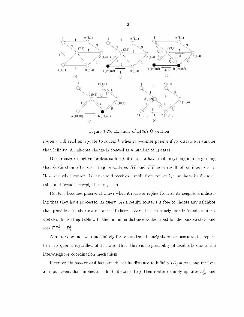
39
(e)
a (1,1)
1
j e (1,1)
b (3,3)
d (2,2)
1
99
8
1
1
5
1
(a)
j 1 e (1,1)
9
1
b (3,3)a (inf,inf)
8
95
d (2,2)
1
Q
Q c (4,4)
(b)
c (4,4)
a (inf,inf) b (inf,inf)
c (4,4)
e (1,1)j
d (9,2)9
5
Q Q
Q, R
UR
UU
(c)
b (inf,inf)
e (1,1)j
c (10,4)
a (10,10) R
9
RR
U
U
U
e (1,1)
c (10,4)
a (10,10) b (10,10)
d (9,2)d (9,2)
j1
95
18
1
U
U
U
1
1
(d)
Figure 3.25: Example of LPA's Operation
router i will send an update to router k when it becomes passive if its distance is smaller
than in�nity. A link-cost change is treated as a number of updates.
Once router i is active for destination j, it may not have to do anything more regarding
that destination after executing procedures RT and DT as a result of an input event.
However, when router i is active and receives a reply from router k, it updates its distance
table and resets the reply ag (rijk = 0).
Router i becomes passive at time t when it receives replies from all its neighbors indicat-
ing that they have processed its query. As a result, router i is free to choose any neighbor
that provides the shortest distance, if there is any. If such a neighbor is found, router i
updates the routing table with the minimum distance as described for the passive state and
sets FDij = Di
j .
A router does not wait inde�nitely for replies from its neighbors because a router replies
to all its queries regardless of its state. Thus, there is no possibility of deadlocks due to the
inter-neighbor coordination mechanism.
If router i is passive and has already set its distance to in�nity (Dij =1), and receives
an input event that implies an in�nite distance to j, then router i simply updates Dijk and

40
dik and sends a reply to router k with an in�nite distance if the input event is a query
from router k. This ensures that updates messages will stop when a destination becomes
unreachable.
Figure 3.25 illustrates LPA's interneighbor coordination mechanism. The number ad-
jacent to each link represents the weight of that link; U indicates updates, Q represents
queries and R replies. The arrowhead from node x to node y indicates that node y is the
successor of node x towards destination j; i.e., sxj = y. The label in the parenthesis assigned
to node x indicates current distance (Dxj ) and the feasible distance from x to destination j
(FDxj ). Active nodes are indicated in black.
In the example (Figure 3.25), we assume that messages propagate across all links at the
same speed, which is considered a step. Nodes process all messages received in the previous
step in zero time.
When link (a; j) fails, node a updates its distance table by setting the distances from d
and b to j equal to 1, because the paths to j reported by both b and d include a. After
that, node a is unable to �nd a feasible successor to j, because Dajb = Da
jd =1 > 1 = FDaj .
Accordingly, it sends a query to all its neighbors (Figure 3.25(b)).
When node d receives a's query, it updates its distance table as follows: it sets Ddja =1
because a reports Daj =1, and it sets Dd
jb = Ddjc =1, because the paths to j reported by
b and d include node a. Because d uses a to reach j, d must also update its routing table.
After updating its distance table, the neighbor that o�ers the shortest distance to j is j
itself. Furthermore, Ddjj = 0 < 2 = FDd
j , and d sends an update to all its neighbor with
Ddj = 1 + 9 = 10 and a reply to node a (Figure 3.25(c)).
When node b receives a's query (before receiving a new update from d), it must set
Dbja = Db
jd = Dbjc = 1, because all its neighbors have reported a path to j that include
node a. Because b's own path to j includes node a, it must update its routing table. Node
b sends a query to its neighbors because every distance to j through any neighbor is in�nity
(Figure 3.25(c)).

41
When a receives the replies from d and b, it makes node d its new successor and also
sends a reply to b (Figure 3.25(d)). When c receives the update from d and the query from
b, it makes e its successor, because Dcje = 1 < 4 = FDc
j and e o�ers the shortest path to j
among all of c's neighbors. Accordingly, c sends an update with its new distance of 10 and
a reply to b's query.
Finally, when b receives all the replies to its queries, it sets d as its successor and sends
updates accordingly (Figure 3.25(e)).
Ensuring Simple Paths
Before updating the routing table, the algorithm ensures that all �nite distances in the
routing table corresponds to a simple path by allowing router i to select as the successors
to destination only neighbors that satisfy the following property:
Property 1 Router i sets sij = k at time t only if Dixk(t) + dik(t) � Di
xp(t) + lip(t) for
every neighbor p other than k and for every node x in the path from i to j de�ned by the
predecessors reported by neighbor k.
Let P ijk(t) denote the path from k to j de�ned by the predecessors reported by neighbor
k to router i and stored in router i's distance table at time t. Procedure TRT enforces Prop-
erty 1 by traversing all or part of P ijk(t) from j back to k using the predecessor information.
This path traversal ends when either a predecessor x is reached for which tagix = correct or
error, or neighbor k is reached. If tagix = error, then tagij is set to error also; otherwise, the
neighbor k or a correct tag must be reached, in which case tagij is set to correct. Lemma 3.2
shows that this traversal correctly enforces Property 1, without having to traverse an entire
implicit path; as the simulation results presented in Section 3.2.3 show, this makes LPA
considerably more e�cient than other prior path �nding algorithms [CRKGLA89, Hum91].
Handling Topology Changes
When router i establishes a link with a neighbor k, it updates its link-costs table and
assumes that router k has reported in�nite distances to all destinations and has replied to
42
any query for which router i is active; furthermore, if router k is a previously unknown
destination, router i initializes the path information of router k and sends an update to
the new neighbor k for each destination for which it has a �nite distance. When router i
is passive and detects that link (i; k) has failed, it sets dik = 1, Dijk = 1 and pijk = null;
after that, router i carries out the same steps used for the reception of a link-cost change
message in passive state. When router i is active and loses connectivity with a neighbor
k, it resets the reply ag and resets the path information i.e., assumes that the neighbor k
sent a reply reporting an in�nite distance.
It follows from this description of router i's operation that the order in which router i
processes updates, queries and replies does not change with the establishment of new links
or link failures. The addition or failure of a router is handled by its neighbors as if all the
links connecting to that router were coming up or going down at the same time.
LPA is loop-free at every instant. This is possible by the single-hop interneighbor
coordination and the e�cient updating mechanism. The details of the proofs of loop-freedom
of LPA are given in [GLAM96]. LPA has been shown to have a worst-case complexity of
O(x) after a single resource failure, where x is the number of routers a�ected in the topology
change. This is also made possible by the e�cient updating mechanism used to update the
distance table entries in LPA.
3.2.2 Correctness of LPA
To prove that LPA converges to correct routing-table values in a �nite time, we assume
that there is a �nite time Tc after which no more link-cost or topology changes occur.
Lemma 3.1 LPA is live.
Proof: Consider the case in which the network has a stable topology. When a router is
in the active state and receives a query from a neighbor, the router replies to the query with
an in�nite distance. The router updates its distance table entries when either an update
or a reply message is received in active state. On the other hand, when a router in passive
state receives a query from its neighbor, it computes the feasible distance and updates its

43
distance and routing tables accordingly. If the router �nds a feasible successor, it replies
to its neighbor's query with its current distance to the destination. If the router can �nd
no feasible successor, it forwards the query to the rest of its neighbors and sends a reply
with an in�nite distance to the neighbor who originated the query. Accordingly, in a stable
topology, a router that receives a query from a neighbor for any destination must answer
with a reply within a �nite time, which means that any router that sends a query in a stable
topology must become passive after a �nite time.
Consider now the case in which the network topology changes. When a link fails or is
reestablished, an active router that detects the link status change simply assumes that the
router at the other end of the link has reported an in�nite distance and has replied to the
ongoing query. Because an active router must detect the failure or establishment of a link
within a �nite time, and because router failures or additions are treated as multiple link
failures or additions, it follows from the previous case that no router can be active for an
inde�nite period of time and hence the lemma is true. 2
Lemma 3.2 TRT correctly enforces Property 1.
Proof: TRT correctly enforces Property 1 if the tag value given by TRT at router i for
destination j equals correct. This is true only when the neighbor n that router i chooses as
successor to j o�ers the smallest distance from i to each node in its reported implied path
from n to j.
First note that, procedure DT is executed before TRT and ensures that router i sets
Dijb = 1 if its neighbor b reports a path to b that includes i. Therefore, TRT deals with
simple paths only.
According to procedure TRT, there are two cases in which a router stops tracing the
routing table (a) the trace reaches node i itself (i.e., pixns = i), and (b) a node on the path
to j is found with tagix = correct. We prove that the correct path information is reached in
both cases.
Case 1: Assume that TRT is executed for destination j after an input event. The tag for
each destination a�ected by the input event is set to null before procedure TRT is executed.

44
Therefore, if TRT is executed for destination j and node i (the source) is reached, the tag of
each node in the path from i to j through neighbor n must be null. Therefore, the distance
from i to j through n is the shortest path among all neighbors since node i chooses the
minimum in row entry among its neighbors for a given destination j. The lemma is true
for this case.
Case 2: If node x1 with tagix1
= correct is reached, then it must be true that either node
i or a node x2 with tagix2 = correct is reached from x1.
If node i is reached from x1, then it follows from Case 1 that neighbor n o�ers the
smallest distance among all of i's neighbors to each node in the implied subpath from n to
x1 reported by neighbor n. Furthermore, because x1 is reached from j, node n must also
o�er the smallest distance among all of i's neighbors to each node in the implied subpath
from x1 to j reported by n. Therefore, it follows that the lemma is true if node i is reached
from x1 (from Case 1). Otherwise, if x2 is reached, the argument used when i is reached
from x1 can be applied to x2. Because router i always sets tagii = correct and TRT deals
with simple paths only, this argument can be applied recursively only for a maximum of
h <1 times until i is reached, where h is the number of hops in the implicit path from n
to j reported by n to i. Therefore, Case 2 must eventually reduce to Case 1 and it follows
that the lemma is true. 2
Lemma 3.3 The change in the cost or status of a link will be re ected in the distance and
the routing tables of a router adjacent to the link within a �nite time.
Proof: Regardless of the state in which router i is for a given destination j, it updates
its link-cost and distance table within a �nite time after it is noti�ed of an adjacent link
changing its cost, failing, or starting up. On the other hand, router i is allowed to update its
routing table for destination j only when it is in passive state for that destination. However,
because LPA is live (Lemma 1), if router i is active for destination j, it must receive all the
replies to its query regarding j within a �nite time, i.e., when it becomes passive. When
router i becomes passive for destination j, it executes Procedure TRT, which updates the
routing-table entry for destination j using the most recent information in router i's distance

45
table. This implies that any change in a link is re ected in the distance and routing tables
of a neighbor router within a �nite time T . 2
Given Lemma 3.3 and our assumption about time Tc, a �nite time must exist when all
routers adjacent to the links that changed cost or status have updated their link cost and
status information, and after which no more link-cost or topology changes occur. Let T
denote that time, where Tc � T <1.
Theorem 1 After a �nite time t � T , the routing tables of all routers must de�ne the �nal
shortest path to each destination.
Proof: Let T (H) be the time at which all messages sent by routers with shortest paths
having H�1 hops (H � 1) to a given destination j have been processed by their neighbors.
Assume that destination j is reachable from every router.
For any router a adjacent to j, it follows from Lemma 2 that, if router a's shortest path
to j is the link (a; j), then router a must update Daj = daj by time T = T (0) and the
theorem is true for H = 0.
Because LPA is loop free at every instant (Theorem 1), the number of hops in any
shortest path (as implied by the successor graph) is �nite. Accordingly, the proof can
proceed by induction on H .
Assume that the theorem is true for some H > 0. According to this inductive assump-
tion, by time T (H), router i must have a correct routing-table entry for every destination
for which it has a shortest path of H hops or less. Property 1 must be satis�ed for all
such destinations and LPA enforces it correctly (Lemma 3.2). On the other hand, from the
de�nition of T (H + 1), it follows that any update messages sent by routers with shortest
paths of H hops or less to j or any other destination have been processed by their neighbors
by time T (H + 1). Therefore, if router i's shortest path to destination j has H + 1 hops,
Property 1 must be satis�ed at router i for that destination by time T (H + 1), because all
possible predecessors for destination j must satisfy Property 1 at router i and that router
must have the correct information for link (i; sij) at time T (0) < T (H + 1) (Lemma 3.2). It
follows that the theorem is true for the case of a connected network.

46
Consider the case in which j is not accessible to a connected component C of the network.
Assume that there is a router i 2 C such that Dij <1 at some arbitrarily long time. If that
is the case, j must satisfy Property 1 through at least one of router i's neighbors at that
time; the same applies to such a neighbor, and to all the routers in at least one path from i
to j de�ned by the routing tables of routers in C. This is not possible, because C is �nite
and LPA is always free of loops and live, which implies that, after a �nite time tf � T , all
paths to j de�ned by the successor entries in the routing tables of routers in C must lead
to routers that have set their distance to j equal to1. Therefore, because C is �nite, LPA
is live, and messages take a �nite time to be transmitted, it follows that destination j will
fail to satisfy Property 1 at each router within a �nite time t � tf , and routers must then
set their distances to in�nity, and the theorem is true. 2
Theorem 2 A �nite time after t, no new update messages are being transmitted or pro-
cessed by routers in G, and all entries in distance and routing tables are correct.
Proof: After time T , the only way in which a router can send an update message is after
processing an update message from a neighbor. Accordingly, the proof needs to consider
three cases, namely: router i receives an update, a query, or a reply from a neighbor.
Consider an arbitrary router i 2 G. Because LPA is live (Theorem 1) and router i
obtains its shortest distance and corresponding path information for destination j in a
�nite time after T (Theorem 2), router i must be passive within a �nite time ti � T .
If router i receives an update for destination j from router k after time ti, router i must
execute Procedure Update. If router i has no path to destination j, Dij must be in�nity
and router k must report an in�nite distance as well, because router i achieves its �nal
shortest-path at time ti; in this case, router i simply updates its distance table. On the
other hand, if router i has a path to destination j, then Dij <1 and router i must �nd that
FC is satis�ed and execute Procedure TRT. Because an update entry is added only when
the shortest distance or predecessor to j change, router i can send no update or query of
its own.

47
If router i receives a query from a neighbor for destination j after time ti, it must execute
Procedure Query. If router i has no physical path to destination j, Dij must be in�nity and
router k must report an in�nite distance in its query, because router i achieves its �nal
shortest-path at time ti; in this case, router i simply updates its distance table and sends
a reply to router k with an in�nite distance. On the other hand, if router i has a physical
path to destination j, it must determine that FC is satis�ed when it processes router k's
query. Accordingly, it simply sends a reply to its neighbor with its current distance and
predecessor to router j. Therefore, router i cannot send an update or query of its own when
it processes a query from a neighbor after time ti.
After time ti, router i cannot receive a reply from a neighbor, unless it �rst sends a
query after time ti, which is impossible according to the above two paragraphs.
It follows from the above that, for any given destination, no router in G can generate
a new update or query after it reaches its �nal shortest path and predecessor to that
destination. Because every router must obtain its �nal shortest distance and predecessor
to every destination within a �nite time (Theorem 2), the theorem is true. 2
3.2.3 Simulation Results
The performance of LPA was compared with that of DUAL and ILS. Simulation environ-
ment and instrumentation are as described in Section 3.1.2 and 3.1.3 respectively. Here,
we focus our simulation study on Arpanet topology. We have studied the performance of
the algorithm for single resource failures and recoveries and for random link cost changes.
For random link-cost changes, links were chosen at random, with link costs chosen from
the interval (0,1] and with a Poisson distributed interarrival time. Five independent runs
were made and the average and the standard deviation of all quantities measured were de-
termined. Interarrival time between the link-cost changes was varied to simulate multiple
link-cost changes.
The link model allows the link delay to be set independently for each link. Each unit of
time represents a step in which all currently available packets are processed. Although the

48
10
100
1000
0 10 20 30 40 50 60 70
ME
SS
AG
ES
LINK FAILURES
LPADUAL
ILS
Figure 3.26: ARPANET Link Failure
0
50
100
150
200
250
0 10 20 30 40 50 60 70
ME
SS
AG
ES
LINK RECOVERIES
LPADUAL
ILS
Figure 3.27: ARPANET Link Recovery
10
100
1000
0 5 10 15 20 25 30 35 40 45 50
ME
SS
AG
ES
NODE FAILURES
LPADUAL
ILS
Figure 3.28: ARPANET Node Failure
0
50
100
150
200
250
300
350
400
450
0 5 10 15 20 25 30 35 40 45 50
ME
SS
AG
ES
NODE RECOVERIES
LPADUAL
ILS
Figure 3.29: ARPANET Node Recovery
choice of input parameters causes the simulation to proceed synchronously, the node model
treats each incoming packet asynchronously. Each input event is processed independently
of other events received during the same simulation step.
The graphs in Figures 3.26 and 3.27 depicts the performance of the routing algorithms
for a single topology change. The graphs show the number of messages exchanged before
LPA, DUAL and ILS converge for every link failing and recovering in the Arpanet topology
respectively. Similar graphs for each node failing and recovering are given in Figures 3.28
and 3.29, respectively. All topology changes were performed one at a time and the algo-
rithms were allowed to converge after each such change before the next resource change

49
Table 3.1: Routing Algorithm Response to a Change in Link Cost
Parameter LPA DUAL ILSmean sdev mean sdev mean sdev
Los-Nettos Cases
Event Count 21.4� 0.47 35.6� 2.8 34.0� 0.24 45.0� 0.54 18.5� 0.05 18.5� 0.04Packet Count 12.2�0.15 7.5� 0.41 15.45� 0.14 18.6� 0.25 17.5� 0.05 17.5� 0.04Duration 3.95� 0.06 1.76� 0.07 4.9�0.06 2.17� 0.07 4.06� 0.01 0.46� 0.03
Operation Count 45.7� 0.23 23.1� 1.1.7 44.0� 0.24 52.9� 0.5 473.9� 3.08 475.5� 3.09
NSFNET Cases
Event Count 34.65� 0.83 72.86� 2.7 50.97� 1.2 68.7� 2.5 28.5� 0.09 28.5� 0.09Packet Count 14.97� 0.15 14.78� 0.47 21.81� 0.54 27.1� 0.82 27.5� 0.1 27.5� 0.09Duration 4.624� 0.05 2.45� 0.05 5.516� 0.17 2.57� 0.15 4.7� 0.02 0.46� 0.01
Operation Count 55.323� 0.4242.64� 1.21 63.97� 1.2 78.8� 2.35 1012.88� 3.9 1014.5� 3.76
ARPANET Cases
Event Count 247.5� 16.09679.7� 24.6 350.09� 15.08501.4� 22.7 84.1� 0.23 84.6� 0.21Packet Count 55.8� 1.86 66.8� 3.0 81.8� 2.99 102.9� 4.9 83.1� 0.23 83.6� 0.21Duration 7.042� 0.22 4.9� 0.09 10.84� 0.45 4.75� 0.55 7.74� 0.028 0.74� 0.022
Operation Count 269.7� 8.05 359.2� 12.2 396.1� 15.1 534.6� 22.6 13613.1� 51.013691.3� 47.4
occurs. The ordinates of the graphs represent the identi�ers of the links and the nodes,
while the data points show the number of messages exchanged after each resource change
in each of these �gures.
The response of the algorithms for a single link-cost change is given in Table 3.1. The
table gives the average value and the standard deviation along with the statistical error for
each link-cost change. The statistical errors were determined based on repeated trails. For
a single link-cost change, LPA is faster and needs fewer messages and operations than both
DUAL and ILS in all topologies. We can conclude from these results that LPA has a better
average performance than ILS and DUAL after any single link-cost or topology change.
Dynamic Response to a Single Change
To study the dynamic behavior of the routing algorithms, we ran an exhaustive series of test
cases for all the node and the link failures and recoveries and recorded the message related
statistics. A statistical characterization of the performance of the routing algorithms was
obtained by treating every node change as a separate case and by computing a distribution
as a function of time. In this section, we present the results of the dynamic behavior of the

50
0.0
0.2
0.4
0.6
0.8
1.0
5 10 15 20 25
PR
OB
AB
ILIT
Y
TIME AFTER LINK FAILURE
LPADUAL
ILS
Figure 3.30: Probability of packets in transitfor Link Failure
0.0
0.2
0.4
0.6
0.8
1.0
2 4 6 8 10 12 14
PR
OB
AB
ILIT
Y
TIME AFTER LINK RECOVERY
LPADUAL
ILS
Figure 3.31: Probability of packets in transitfor Link Recovery
0.0
5.0
10.0
15.0
20.0
25.0
30.0
35.0
5 10 15 20 25
AV
ER
AG
E N
UM
BE
R O
F P
AC
KE
TS
TIME AFTER LINK FAILURE
LPADUAL
ILS
Figure 3.32: Average number of packets forLink Failure
0.0
5.0
10.0
15.0
20.0
25.0
30.0
35.0
2 4 6 8 10 12 14
AV
ER
AG
E N
UM
BE
R O
F P
AC
KE
TS
TIME AFTER LINK RECOVERY
LPADUAL
ILS
Figure 3.33: Average number of packets forLink Recovery
0.0
0.2
0.4
0.6
0.8
1.0
0 5 10 15 20 25 30 35 40 45 50
PR
OB
AB
ILIT
Y
TIME AFTER NODE FAILURE
LPADUAL
ILS
Figure 3.34: Probability of packets in transitfor Node Failure
0.0
0.2
0.4
0.6
0.8
1.0
0 5 10 15 20
PR
OB
AB
ILIT
Y
TIME AFTER NODE RECOVERY
LPADUAL
ILS
Figure 3.35: Probability of packets in transitfor Node Recovery
routing algorithms for the Arpanet topology. In the instrumentation, we do not consider
paths from a node to itself, because they do not require a network. In our simulations, we
have taken care to handle these cases.

51
Figures 3.30{3.37 show the transient response of the routing algorithms (probability of
packets in transit and the average number of messages that are exchanged) after a link
failure, link recovery, node failure and node recovery respectively. These are shown as a
function of time.
The results indicate that for a link failure, ILS performs better than DUAL and LPA
in terms of the number of messages exchanged. LPA's average performance is much better
than ILS for resource addition at any time after the change. The performance of LPA
is comparable to ILS after a node failure. In all cases, LPA outperforms DUAL. The
probability of packets being in transit for LPA after a resource recovery is less than ILS
and DUAL. The average packet length for LPA after a resource change is much smaller
than DUAL. This is because of the single hop interneighbor coordination mechanism and
the tagging mechanism used in LPA.
Response to Multiple Link-Cost Changes
The steady-state behavior of the algorithms is more interesting with multiple link-cost
changes than the transient response after each topology change. Figures 3.38{3.41 shows
the average number of update messages when such messages are in transit, the average
lengths of messages, the average number of messages in transit and the probability that the
messages are in transit as a function of the interarrival times between link-cost changes for
LPA, DUAL and ILS. This again is for the Arpanet topology. From [ZGLA92], it has been
observed that the behavior of DUAL and ILS for multiple link-cost changes is similar for
di�erent network topologies; our conjecture is that the same is true for LPA.
For very long interarrival times, the number of messages during busy periods is inde-
pendent of the interarrival time because the probability of two topology changes occurring
simultaneously is small. In this case, the performance approaches that of single link-cost
change. When the interarrival time approaches the network diameter, this situation changes
and the number of messages during the busy period increases because of multiple topology
changes occurring simultaneously.

52
0.0
10.0
20.0
30.0
40.0
50.0
60.0
0 5 10 15 20 25 30 35 40 45 50
AV
ER
AG
E N
UM
BE
R O
F P
AC
KE
TS
TIME AFTER NODE FAILURE
LPADUAL
ILS
Figure 3.36: Average number of packets forNode Failure
0.0
10.0
20.0
30.0
40.0
50.0
60.0
70.0
0 5 10 15 20
AV
ER
AG
E N
UM
BE
R O
F P
AC
KE
TS
TIME AFTER NODE RECOVERY
LPADUAL
ILS
Figure 3.37: Average number of packets forNode Recovery
0.0
0.1
1.0
10.0
100.0
1000.0
1 10 100 1000 10000AV
E N
UM
OF
MS
GS
WH
EN
MS
GS
AR
E IN
TR
AN
SIT
INTERARRIVAL TIME
LPADUAL
ILS
Figure 3.38: Average Number of Messageswhen messages are in Transit
0.10
1.00
10.00
100.00
1 10 100 1000 10000
AV
ER
AG
E M
ES
SA
GE
LE
NG
TH
INTERARRIVAL TIME
LPADUAL
ILS
Figure 3.39: Average Message Length
The average number of messages exchanged when messages are in transit is slightly less
for LPA compared to DUAL and ILS. This again is because of the single-hop internodal
synchronization mechanism and updating of the distance-table entries, which has been
explained earlier. All curves are of roughly the same shape. For ILS, the average message
length is close to 1. DUAL and LPA have longer messages as a message can contain multiple
updates; this occurs when messages from the routers at both ends of a link that changes
cost arrive at some router at the same time. With the increase in the interarrival time
between changes, the average number of messages drops down as it now approaches a single
link-cost change. The average number of messages that are in transit and the probability
that messages are in transit are signi�cantly smaller for LPA compared to DUAL and ILS.
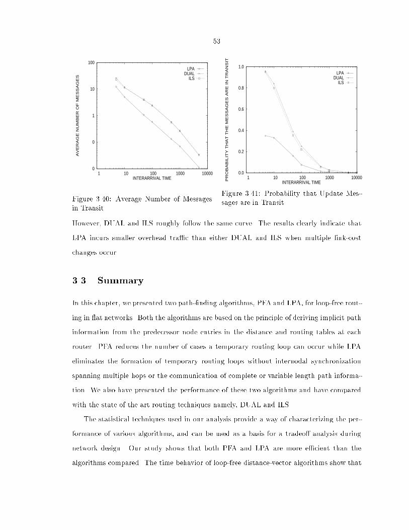
53
0
0
1
10
100
1 10 100 1000 10000
AV
ER
AG
E N
UM
BE
R O
F M
ES
SA
GE
S
INTERARRIVAL TIME
LPADUAL
ILS
Figure 3.40: Average Number of Messagesin Transit
0.0
0.2
0.4
0.6
0.8
1.0
1 10 100 1000 10000PR
OB
AB
ILIT
Y T
HA
T T
HE
ME
SS
AG
ES
AR
E IN
TR
AN
SIT
INTERARRIVAL TIME
LPADUAL
ILS
Figure 3.41: Probability that Update Mes-sages are in Transit
However, DUAL and ILS roughly follow the same curve. The results clearly indicate that
LPA incurs smaller overhead tra�c than either DUAL and ILS when multiple link-cost
changes occur.
3.3 Summary
In this chapter, we presented two path-�nding algorithms, PFA and LPA, for loop-free rout-
ing in at networks. Both the algorithms are based on the principle of deriving implicit path
information from the predecessor node entries in the distance and routing tables at each
router. PFA reduces the number of cases a temporary routing loop can occur while LPA
eliminates the formation of temporary routing loops without internodal synchronization
spanning multiple hops or the communication of complete or variable length path informa-
tion. We also have presented the performance of these two algorithms and have compared
with the state of the art routing techniques namely, DUAL and ILS.
The statistical techniques used in our analysis provide a way of characterizing the per-
formance of various algorithms, and can be used as a basis for a tradeo� analysis during
network design. Our study shows that both PFA and LPA are more e�cient than the
algorithms compared. The time behavior of loop-free distance-vector algorithms show that

54
the parameters such as packet length can change as updates propagate, thereby suggesting
the possibility of heuristics that can exploit local conditions. Our analysis indicates that
overall, LPA and PFA perform signi�cantly better than DUAL and ILS.
In the following chapters, we propose several routing protocols for di�erent networking
environments, which use PFA or LPA as the basic routing algorithm.

55
Chapter 4
A Hierarchical Routing Algorithm
The loop-free path-�nding algorithm (LPA) has been shown to maintain loop-free routing
tables. LPA obtains correct routing tables after topological and link-cost changes faster
and with less processing and communication overhead than link-state algorithms and prior
loop-free routing algorithms based on vectors of distances. The limitation of LPA and prior
routing algorithms based on routing trees is that it requires the routers to maintain more
\host routes" than would be needed in a traditional distance-vector algorithm.
Routing information maintained at each router has to be updated frequently to adapt to
changes in the topology and congestion of the internetwork. In an internetwork with a at
routing structure, the size of the routing tables grow linearly with the number of destinations
in the network. Due to this, the routing information that is required to be maintained at
a node may become excessive in terms of storage and CPU utilization. The information
exchanged among nodes may prove to be expensive in terms of channel bandwidth since
updates need to be exchanged frequently in order to maintain up to date network state
information. Accordingly, aggregation of routing information becomes a necessity in any
type of routing protocol.
For routing in large networks, the aggregation of routing information is achieved through
a hierarchical partitioning of the network. The main idea of hierarchical routing is to main-
tain exact routing information regarding nodes very close to it and less detailed information
regarding nodes that are farther away from it. The goal of maintaining hierarchy of infor-
mation is to reduce the size of the routing database maintained at each router so that the

56
exchange of topology information among the routers can be minimized. The objective of
doing so is to obtain a reasonable compromise among the size of routing tables, number of
updates required to maintain such tables and the speed with which updates are propagated.
In this chapter, we present a hierarchical routing algorithm which we call Hierarchical
Information Path-based Routing (HIPR), which can be used in large systems.
4.1 Prior Work
Hierarchical routing for datagram computer networks was �rst proposed by McQuillan [McQ74]
to reduce the overhead by limiting the amount of routing information each routing node
maintains and to reduce the length of the routing table. In order to reduce the amount
of information maintained at each node and the communication overhead, the network is
organized into clusters or areas by grouping together (clustering) the nodes which are close
by. Each of these clusters is a single addressable entity from the point of view of higher level
clusters. The topology within the area is transparent to the nodes outside the area. The dis-
tance from a source node to an area represents the actual distance in physical hops (number
of nodes traversed) from the source node to the destination remote node. It then becomes
important to determine a speci�c clustering structure, cluster size, and the number of clus-
ters that will result in a minimum table length. Given that an optimal clustering technique
has been determined, an e�cient routing algorithm can be applied to these clusters.
McQuillan [McQ74] proposed an extension to the old Arpanet routing algorithm for
hierarchical networks. This scheme was analyzed by Kamoun and Kleinrock [Kam76]. Ac-
cording to McQuillan, the nodes in the network are organized into m levels of clusters, with
each node belonging to exactly one cluster at each level of the hierarchy. Nodes represent
clusters at level 0; a group of nodes form a cluster at level 1, called 1-cluster; Similarly, a
group of (k � 1) clusters forms a cluster at level k, called a k-cluster. The distance from a
source node to a k cluster represents the length of the shortest-path from the source node to
another node in the k-cluster. Each node maintains a routing table with distance entries to
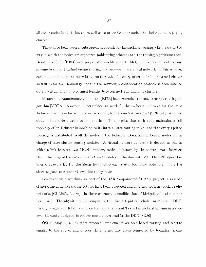
57
all other nodes in its 1-cluster, as well as to other i-cluster nodes that belongs to its (i+ 1)
cluster.
There have been several subsequent proposals for hierarchical routing which vary in the
way in which the nodes are organized (addressing scheme) and the routing algorithms used.
Baratz and Ja�e [BJ83] have proposed a modi�cation to McQuillan's hierarchical routing
scheme to support virtual-circuit routing in a two-level hierarchical network. In this scheme,
each node maintains an entry in its routing table for every other node in its same l-cluster
as well as for each boundary node in the network; a collaboration protocol is then used to
obtain virtual circuit to optimal lengths between nodes in di�erent clusters.
Meanwhile, Ramamoorthy and Tsai [RT83] have extended the new Arpanet routing al-
gorithm [MRR80] to work in a hierarchical network. In their scheme, nodes within the same
1-cluster use intra-cluster updates, according to the shortest-path �rst (SPF) algorithm, to
obtain the shortest paths to one another. This implies that each node maintains a full
topology of its 1-cluster in addition to its intra-cluster routing table, and that every update
message is distributed to all the nodes in the 1-cluster. Boundary or border nodes are in
charge of inter-cluster routing updates. A virtual network at level i is de�ned as one in
which a link between two i-level boundary nodes is formed by the shortest path between
them; the delay of the virtual link is then the delay in the shortest path. The SPF algorithm
is used at every level of the hierarchy to allow each i-level boundary node to compute the
shortest path to another i-level boundary node.
Besides these algorithms, as part of the DARPA-sponsored SURAN project, a number
of hierarchical network architectures have been proposed and analyzed for large packet radio
networks [GLAS85, Lau86]. In these schemes, a modi�cation of McQuillan's scheme has
been used. The algorithms for computing the shortest paths include variations of DBF.
Finally, Seeger and Khanna employ Ramamoorthy and Tsai's hierarchical scheme in a two-
level hierarchy designed to reduce routing overhead in the DDN [SK86].
OSPF [Moy94], a link-state protocol, implements an area-based routing architecture
similar to the above, and divides the Internet into areas connected by boundary nodes
58
linked by a physical backbone. Routing nodes connected to the backbone serve the role of
boundary nodes called backbone nodes or border nodes. Routers not connected to the back-
bone correspond to simple nodes called area nodes. Boundary nodes exchange information
about the backbone links adjacent to them, and area nodes exchange information about
their adjacent intra-area links.
A boundary node reports to other boundary nodes the distance to multiple destinations
in its own area. Topology information about an area is not directly propagated to routers
outside the area. OSPF allows entries in one area to be represented in other areas and
in the backbone as a cost associated with a summary address and a mask. To route to a
destination address, the mask is applied to the address; if it matches the summary address,
the routing-table entry for that summary is used. If there are multiple matches, the most
speci�c is used.
OSPF provides a means to transfer and maintain a set of tables giving the costs of links
and a cost for summary descriptions of distant nodes in the networks. Each boundary node
computes a summary distance for mask/address combinations that match the nodes in each
area attached to the backbone, and sends these distances to other boundary nodes. The
boundary nodes then compute the shortest path to each globally visible node and summary
entry, treating the summary as a link. Boundary nodes also send distances of globally
visible nodes and summarizes outside an area to nodes in that area. The local simple nodes
then treat such a distance as the cost of a link from the boundary node to that destination.
Shortest paths are computed using Dijkstra's shortest-path algorithm for simple nodes and
the boundary nodes.
With very few exceptions [GLAZ94], prior proposals to hierarchical routing have as-
sumed variants of DBF or topology-broadcast algorithms. In the following sections we
present, verify and analyze the performance of the �rst hierarchical routing algorithm
(HIPR) based on the maintenance and exchange of hierarchical routing trees. The main
idea of HIPR consists of providing a distributed implementation of Dijkstra's shortest path
algorithm running over a hierarchical graph organized in areas according to McQuillan's

59
scheme for hierarchical routing. LPA is extended for this purpose. HIPR constitutes the
basis for a new Internet routing protocol that are as simple as RIPv2 [Mal94].
4.2 Network Model
Following the McQuillan's approach to area-based routing, hosts and networks can be orga-
nized into L levels of areas. An area at level k is called a k-area. Each router or destination
belongs to only one area at each level of the hierarchy above level-1 and each k-area is a
proper subset of only one (k + 1)-area. For simplicity, no further mention is made of the
destinations directly attached to routers through LANs or point-to-point links. Hence for
the purposes of discussion, a destination is a router or a k-area.
Routers are themselves 0-areas; a group of nodes forms a 1-area and a group of k-areas
forms (k + 1)-area. A boundary node or a border node is de�ned as a router with direct
connectivity with its peer boundary nodes in areas to which it does not belong. A k-level
border node is the border node that connects k-areas. The distance from a source router
to a remote k area represents the length of the true shortest-path from a node to any
remote area. Clearly, the distance from a router to another router in the same 1-area is the
true shortest path distance. Similarly, the distance from a router to itself (or any directly
adjacent host) is 0 and the distance from the router to its own k-area is 0.
In OSPF terminology, a routing node connected to the backbone network serves as a
boundary node. Routers not connected to the backbone are simple nodes. How the areas
of the network are chosen is outside the scope of this paper, just as the way in which
areas are chosen is not part of the OSPF speci�cation. For example, by taking into account
destination behind routers, masks and subnets, our description of the network hierarchy can
be mapped into a hierarchical addressing scheme that would be practical on an Internet.
For our purposes, it su�ces to illustrate the fact, for HIPR, a destination is a single entity
or an arbitrary aggregation of entities following McQuillan's scheme.

60
C
A2
A3
A1a
d
b
c
BA
Figure 4.1: Example of the Hierarchical Network Topology
d
AA1A1 A
c
A1 A
c
A2
bc
a
C
B
A3
d
c
C
A2
b
A3
B
a
d
a
A3
C
BA2
b
Node d Node cNode a
Figure 4.2: Hierarchical Routing Trees at Nodes
4.3 HIPR
4.3.1 Design Principle
The basic design concept of HIPR is simple. Each router communicates to its neighbors
its hierarchical routing tree in an incremental fashion. Its hierarchical routing tree consists
of all its preferred hierarchical shortest paths to each known individual destinations in its
own 1-area, all known highest-level areas, and in general all (k � 1)-areas within its own
k-area. This means that border nodes forbid detailed routing tree information regarding
their own areas from percolating to other areas. Hence, for a hierarchical routing tree an

61
A2b
c
A2
C
B
A3
(a) Routing Tree sent to neighbor within area A1
(b) Routing Tree sent to areas outside A
(c) Routing Tree sent to areas within area A outside A1
CB
A3
B
C A
a
d
A1A
Figure 4.3: Hierarchical Routing Trees Sent by Border Nodes
entire foreign area is simply another node in the tree. Figures 4.1 and 4.2 illustrates this
idea. Figure 4.1 shows the topology of a network organized hierarchically into three levels,
and Figure 4.2 shows the hierarchical routing tree that router d needs to communicate to its
neighbor routers (within area A1) and the hierarchical routing trees of its two neighbors a
and c. Bold nodes in the trees correspond to \self reference" entries in the router's routing
table. Notice that the path from d to remote areas consists of both routers within router
d's 1-area and other remote areas.
Consider a border node in the given topology (say c). The hierarchical routing tree
propagated to all nodes within the area containing node c is shown in Figure 4.3(a). For
the areas outside the area containing node c (i.e., outside A), the hierarchical routing tree
sent to the peer nodes of other areas is shown in Figure 4.3(b).
Consider border node b in Figure 4.1. This is a border node connecting areas A1 and
A2 which are contained in the bigger area A. The routing tree sent by node b to its peer
border node in area A2 (within area A) is shown in Figure 4.3(c).
Routers exchange their hierarchical routing trees incrementally by communicating only
the hierarchical distance and second-to-last hop (predecessor) to each destination. In the
case of destinations within router d's 1-area, the second-to-last hop consists of a router. In
the case of a remote area known to router d, the predecessor consists of either a border
node in router d's 1-area or a remote area. The hierarchical distance to a destination
consists of the true shortest distance to a border node. The rest of this section describes

62
the information and procedures that HIPR uses to update the hierarchical routing trees of
routers distributedly, examining that no routing table loops are ever formed. In essence,
HIPR implements Dijkstra's shortest-path algorithm distributedly over a hierarchical graph.
Although HIPR supports multiple levels of areas, OSPF can support only two levels
(subnets and backbone). In this paper, we discuss HIPR based on only one level of areas to
simplify its description and because supporting a minimum of one level of areas is critical
for using HIPR as part of an Internet routing protocol, given that, for scalability purposes,
Internet routing protocols maintain routing information about networks (not individual
hosts) and must support subnetting.
4.3.2 Information Maintained at a Router
Each router maintains a single routing table that, for the purpose of the description, can
be thought of as having two parts: a node-level routing table (NRT) and a area level routing
table (ART). The NRT portion of the routing table maintains information about the routers
and destinations in the same area with which a node is a�liated. The ART portion of the
routing table maintains information about other areas (higher-level areas to which a node
belongs). Both parts of the routing table are updated using the same algorithm.
The entry for destination j in node i's NRT consists of the destination's identi�er, the
distance to the destination (Dij), the successor (s
ij), the predecessor (p
ij) along the preferred
path (shortest path) to the destination, and the feasible distance to the destination (FDij),
which we de�ne subsequently. The NRT also maintains a marker (denoted by tagij) used
to update the routing table entries. For destination j, tagij speci�es whether the entry
corresponds to a simple path (tagij = correct), a loop (tagij = error) or a destination that
has not been marked (tagij = null). This marker is used to reduce the number of routing
table entries that need to be processed after each input event impacting the routing table.
ART maintains similar information for each area known to node i.
The distance from a source to destination area (ADij) is the length of the hierarchical
path from source to the destination area. There can be two variations as to how the distance

63
information is maintained. It can be either the hop count to reach a boundary node of the
destination area or it can be the actual distance to reach the boundary node. Hop count
just gives the number of hops required to reach the destination area and does not necessarily
correspond to the actual path length and hence it need not be the shortest path. In our
simulations we have assumed hop counts for simplicity.
The successor entry for the ART is the next area in the path towards the destination
area (Asij) and the predecessor entry (Apij) is the area previous to the destination area. The
successor and the predecessor entries will be null when i determines that the individual or
area destination is unreachable. The ART also maintains a marker (Atagij) for each known
area.
From the above, it is clear that HIPR simply maintains a hierarchical routing tree in a
concise manner.
In addition to its routing table, a router also maintains a distance table, link-cost table
and a reply-status table. Distance table maintained at each router is a matrix containing
for each destination j, the hierarchical routing tree reported by its neighbors k 2 Ni. At
router i, Dijk and pijk represents the distance and the predecessor reported by neighbor k
for destination j respectively.
The link-cost table contains the cost of each link adjacent to the node maintaining the
table. The cost of the link is denoted by lik. The cost of an inactive link is set to in�nity.
The reply-status table at node i maintains the values of the reply status ag (rijk) for
each neighbor, k, and for each known destination and area, j, to node i. Each entry in this
table indicates whether or not a node is waiting to get a reply from its neighbor in response
to its query.
4.3.3 Information Exchanged between Nodes
Routing information is exchanged among neighboring nodes by means of update messages.
An update message from router i consists of a vector of entries reporting incremental updates
of its routing table; each entry speci�es an update ag (denoted by uij), a destination j (i.e.,
64
an individual node or an area), the reported distance to that destination, and the reported
predecessor (individual node or an area) in the path to the destination. The update ag
indicates whether the entry is an update (uij = 0), a query (uij = 1) or a reply (uij = 2).
The distance in a query is always set to 1.
Because every router reports to its neighbors the second-to-last hop in the shortest path
to the destination, the complete path to any destination (called the implicit path to the
destination) is known by the router's neighbors. This is done by the path traversal on the
predecessor entries reported by the router.
In the speci�cation of HIPR, the successor to destination j for any router is simply
referred to as the successor of the router. Same reference applies to other information
maintained by the router. Similarly, updates, queries and replies refer to destination j
unless otherwise stated.
Figures 4.4 and 4.5 specify HIPR. The procedures used for initialization are Init1 and
Init2; procedure Message is invoked when a router processed a message. Procedures linkup,
linkdown and linkchange, which are referred to as event-handling procedures, are executed
when a router detects a new link, the failure of a link or the change in the cost of a link.
Procedure Message calls Update, Query or Reply to handle an update, a query or a reply
respectively. An important characteristic of all event-handling procedures is that they mark
tagij = null for each destination j a�ected by the input event.
The information propagated to the neighbor depends on whether the node is a border
node or not. Border nodes block any information about its local area before sending an
update to other border nodes (in its peer areas). This ensures that the algorithm is scalable.
Router i initializes itself in passive state with an in�nite distance for all its known
neighbors and with a zero distance to itself. After initialization, router i sends updates
containing the distance to itself to all its neighbors.
4.3.4 Distance Table Updating
The procedures used in HIPR to update the entries of the distance tables are similar to the
procedures used in LPA [GLAM95]. The key di�erence is that, as we have stated, a border

65
Procedure Init1when router i initializes itselfdo begin
set a link-state table withcosts of adjacent links;N fig;Ni fx j dix <1g;initialize Ai;for each (x 2 Ni)do begin
N N [ x; tagix null;
six null; pix null;
Dix 1; FDix 1endfor each (y 2 Ai)do begin
Atagiy null; ADiy 1;
Apiy null; Apiy null;
end
sii i; pi
i i; tagi
i correct;
Dii 0; FDi
i 0;
for each j 2 N call Init2(x, j);for each (n 2 Ni) doadd (0, i, 0, i) to LISTi(n);for each (n 2 Ai) doadd (0, i, 0, i) to LISTi(n);call Send
end
Procedure Query(j, k)begin
if (rijx
= 08x 2 Ni)
then begin
if (Dij= 1 and Di
jk= 1)
then add (2, j, Dij, pij)
to LISTi(k)else begin
call Passive Update(j);
add (2, j, Dij, pij)
to LISTi(k);end
else call AU(j, k)end
Procedure Update(j, k)begin
if (rijx
= 0; 8x 2 Ni)
then begin
if ((sij= k) or (Di
jk< Di
j))
then call Passive Update(j)endelse call AU(j, k)
end
Procedure Init2(x, j)begin
Dijx 1; pi
jx null;
sijx null; ri
jx 0;
end
Procedure Messagewhen router i receives a messageon link (i; k)
begin
for each entry (ukj; j;RDk
j; rpk
j)
such that j 6= i
do beginif (j 62 N)then begin
if (RDkj=1)
then delete entryelse begin
N N [ fjg; FDij=1;
for each x 2 Nicall Init2(x, j)
tagij null;
call DT Update(j;k)end
endelse
tagij null; call DT Update(j; k)
end
for each entry (ukj; j;RDk
j; rpk
j) left
such that j 6= i
do case of value of uij
0: [Entry is an update]call Update(j, k)
1: [Entry is a query]call Query(j, k)
2: [Entry is a reply]call Reply(j, k)
endcall Send
end
Procedure Reply(j, k)begin
rijk 0;
if (rijn
= 0; 8n 2 Ni)
then if ((9x 2 Ni j Dijx
<1)
or (Dij<1))
then call Passive Update(j)else call Active Update(j, k)
end
Procedure Sendbegin
if (i is not a border node)begin
for each (n 2 (Ni [ Ai))do begin
if (LISTi(n) is not empty)then send message withLISTi(n) to n
empty LISTi(n)end
endelse begin
for each (n 2 Ai)do begin
if (LISTi(n) is not empty)then send message withLISTi(n) to n
empty LISTi(n)end
endend
Procedure Passive Update(j)begin
DTmin MinfDijx8 x 2 Nig;
FCSET fn j n 2 Ni; Dijn
= DTmin,
Dnj< FDi
jg;
if (FCSET 6= ;) then begincall RT Update(j, DTmin);
FDij MinfDi
j; FDi
jg
endelse begin
FDij= 1; ri
jx= 1; 8x 2 Ni ;
Dij= Di
j sij
;
pij= pi
j sij
;
if (Dij=1) then si
j null;
8 x 2 Ni do beginif (query and x = k)
then rijk 0;
else add (1, j, 1, null)to LISTi(x)
endend
end
Figure 4.4: HIPR Speci�cation
node at level k running HIPR supports hierarchical routing by making sure that no routing
information regarding destinations in its own 1-area or any (k � 1)-area in its own k-area
percolates to a neighbor border node in another k-area.
When router i receives an input event regarding neighbor k indicating the change in the
link cost (i; k), it updates its link-cost table with the new cost of the link and then updates
the distance table entries making sure that the implicit paths after the changed state of the
network does not imply any loops. Updating the distance table entries erases the outdated
path information by making the path information consistent with the latest update. This is

66
Procedure Link Up (i; k; dik)when link (i; k) comes up do begin
dik cost of new link;if (k 62 N) then begin
N N [ fkg; tagik null;
Dik 1; FDi
k 1;
pik null; si
k null;
for each x 2 Ni do call Init2(x, k)endNi Ni [ fkg;for each j 2 N do call Init2(k, j);
for each j 2 N � k j Dij<1 do
add (0, j, Dij, pij) to LISTi(k);
call Sendend
Procedure Link Down(i; k)when link (i; k) fails do begin
dik 1;for each j 2 N do begin
call DT Update(j, k);
if (k = sij) then tagi
j null
enddelete column for k in distance table;Ni Ni � fkg;
delete rijk
;
for each j 2 (N � i) j k = sij
call Update(j, k)call Send
end
Procedure Active Update(j, k)begin
if (k = sij) then begin
Dij Di
jk; pi
j pi
jk;
endend
Procedure DT Update(j; k)begin
Dijk RDk
j+ dik ; p
ijk rpk
j;
for each neighbor b do beginh j;
while (h 6= i or k or b) do h pbh;
if (h = k) then begin
Dijb Di
kb+ RDk
j; pijb rpk
j;
endif (h = i) then begin
Dijb 1; pi
jb null;
endend
end
Procedure Link Change (i; k; dik)when dik changes value do begin
old dik ;dik new link cost;for each j 2 N do begin
call DT Update(j, k);for each j 2 N
do if (Dij> Di
jkor k = si
j)
then tagij null;
endfor each j 2 N do begin
if (dik < old)
then for each j 2 N � i j Dij> Di
jkdo call Update(j, k)
else for each j 2 N � i j k = sij
do call Update(j, k)endcall Send
end
Procedure RT Update(j, DTmin)begin
if (Dij si
j
= DTmin)
then ns sij;
else ns b j fb 2 Ni and Dijb
= DTming;
x j;
while (Dix ns = MinfDixb8 b 2 Nig
and (Dixns <1) and (tagix = null))
do x pix ns;
if (pix ns = i or tagix = correct)
then tagij correct;
else tagij error;
if (tagij= correct)
then begin
if (Dij6= DTmin or pi
j6= pi
j ns)
then add (0, j, DTmin , pij ns
)
to LISTi(x) 8x 2 Ni;
Dij DTmin; p
ij pi
j ns;
sij ns;
endelse begin
if (Dij<1)
then add (0, j, 1, null)to LISTi(x) 8x 2 Ni ;
Dij 1; pi
j null;
sij null;
endend
Figure 4.5: HIPR Speci�cation (cont...)
done by updating the distance and predecessor information for each destination j a�ected
by the input event (Dijk = Dk
j + dik and pijk = pik). In addition to this, the path to any
destination j through any other neighbor which includes neighbor k is also updated. This is
done by traversing the path speci�ed by the predecessor entries reported by a neighbor from
destination j towards node i. If the path implied by the predecessor reported by router b
(b 6= k and b 2 Ni) to destination j includes router k, then the distance and predecessor
entries are updated for that path.
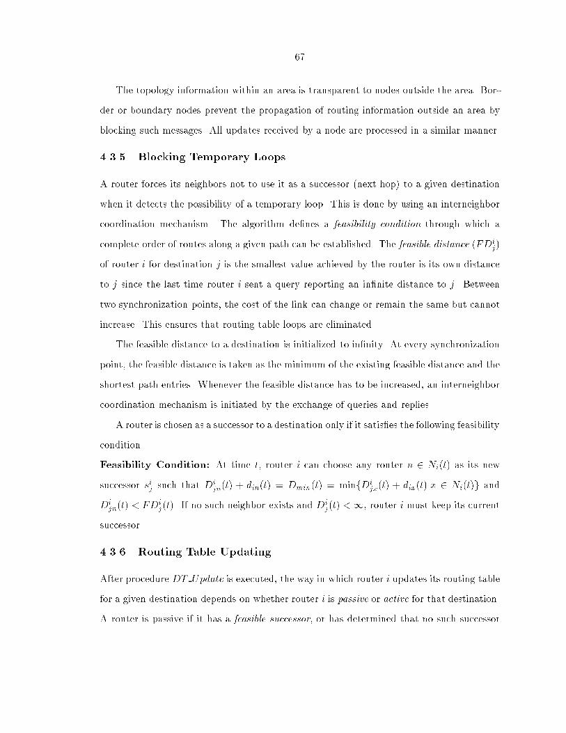
67
The topology information within an area is transparent to nodes outside the area. Bor-
der or boundary nodes prevent the propagation of routing information outside an area by
blocking such messages. All updates received by a node are processed in a similar manner.
4.3.5 Blocking Temporary Loops
A router forces its neighbors not to use it as a successor (next hop) to a given destination
when it detects the possibility of a temporary loop. This is done by using an interneighbor
coordination mechanism. The algorithm de�nes a feasibility condition through which a
complete order of routes along a given path can be established. The feasible distance (FDij)
of router i for destination j is the smallest value achieved by the router is its own distance
to j since the last time router i sent a query reporting an in�nite distance to j. Between
two synchronization points, the cost of the link can change or remain the same but cannot
increase. This ensures that routing table loops are eliminated.
The feasible distance to a destination is initialized to in�nity. At every synchronization
point, the feasible distance is taken as the minimum of the existing feasible distance and the
shortest path entries. Whenever the feasible distance has to be increased, an interneighbor
coordination mechanism is initiated by the exchange of queries and replies.
A router is chosen as a successor to a destination only if it satis�es the following feasibility
condition.
Feasibility Condition: At time t, router i can choose any router n 2 Ni(t) as its new
successor sij such that Dijn(t) + din(t) = Dmin(t) = minfDi
jx(t) + dix(t)jx 2 Ni(t)g and
Dijn(t) < FDi
j(t). If no such neighbor exists and Dij(t) <1, router i must keep its current
successor.
4.3.6 Routing Table Updating
After procedure DT Update is executed, the way in which router i updates its routing table
for a given destination depends on whether router i is passive or active for that destination.
A router is passive if it has a feasible successor, or has determined that no such successor

68
exists and is active if it is searching for a feasible successor. A feasible successor for router
i with respect to destination j is a neighbor router that satis�es FC.
When router i is passive, it reports the current value of Dij in all its updates and replies.
While router i is active, it sends an in�nite distance in its replies and queries. An active
router cannot send an update regarding the destination for which it is active, because
any update sent during active state would necessarily have to report an in�nite distance
to ensure the correct operation of the inter-neighbor synchronization mechanism used in
HIPR.
If router i is passive when it processes an update for destination j, it determines whether
or not it has a feasible successor, i.e., a neighbor router that satis�es FC.
If router i �nds a feasible successor, it sets FDij equal to the smaller of the updated
value of Dij and the present value of FDi
j . In addition, it updates its distance, predecessor,
and successor making sure that only simple paths are used.
Router i then prepares an update message to its neighbors if its routing table entry
changes. Alternatively, if router i �nds no feasible successor, then it sets FDij = 1 and
updates its distance and predecessor to re ect the information reported by its current
successor. If Dij(t) =1, then sij(t) = null. Router i also sets the reply status ag (rijk = 1)
for all k 2 Ni and sends a query to all its neighbors. Router i is then said to be active, and
cannot change its path information until it receives all the replies to its query.
The tagging mechanism used for routing table updating ensures that only those routing
table entries a�ected by the input event will be traversed and updated. i.e., if there is a
topology change in the existing routing tree then, only nodes which are downstream to that
topological change need to be updated since this change does not a�ect nodes upstream to
the topological change. This mechanism minimizes the processing that has to be done for
each update message.
A path P ijk(t) is de�ned by the predecessors reported by neighbor k to router j stored
in i's distance table at time t. To ensure loop-free paths, path traversal from j back to k is
made using the predecessor information. Complete or partial path can be traversed. Path

69
traversal ends when either a predecessor x for which tagix = correct or tagix = error or
neighbor k is reached. If tagix = error, then tagij is set to error also; otherwise, the neighbor
k or a correct tag must be reached in which case tagij is set to correct. This mechanism
ensures loop-free paths without having to traverse the entire routing table.
4.3.7 Processing of Queries and Replies
Queries and replies are processed in a manner similar to the processing of an update, as
described above. If the input event that causes router i to become active is a query from its
neighbor k, router i sends a reply to router k reporting an in�nite distance. This happens
because router k's query, by de�nition, reports the latest information from router k, and
router i will send an update to router k when it becomes passive if its distance is smaller
than in�nity. A link-cost change is treated as a link failing and recovering with a new link
cost.
When router i is active and receives replies from all its neighbors, it resets the reply
ag (rijk = 0). This means that router i's neighbors have processed the query reporting
an in�nite distance. Therefore, router i is free to choose any neighbor that provides the
shortest distance, if there is any. If such a neighbor is found, router i updates the routing
table with the minimum distance and sets FDij = Di
j .
A router does not wait inde�nitely for replies from its neighbors because a router replies
to all its queries regardless of its state. Thus, there is no possibility of deadlock due to the
inter-neighbor coordination mechanism.
If router i is passive and has already set its distance to in�nity (Dij =1), and receives
an input event that implies an in�nite distance to j, then router i simply updates Dijk and
dik and sends a reply to router k with an in�nite distance if the input event is a query
from router k. This ensures that updates messages will stop when a destination becomes
unreachable.

70
4.3.8 Example
Consider the topology with three areas, A, B and C in Figure 4.1. We concentrate on
area A1 which contains a four-node network. Area A1 has three border nodes, a, b and c
through which it is connected to areas A3 (and B), A2 and C, respectively. To simplify
the description of how HIPR operates, a \virtual topology" of areas and routers is shown
in Figure 4.6 (a). This topology consists of the destinations known to routers in area A1
and the links between destinations that may be known to the routers in area A1 depending
on their routing trees. This is an eight-node topology, with each node representing either
a node or an area. A link to an area indicates the existence of a link from a border node
outside the area to a border node inside the area. A node indicating an area represents
the border node(s) that provides inter-area connectivity to the area. Message sent by an
\area node" over a link corresponds to messages sent by the corresponding border node.
We explain the working of HIPR on this topology when the link connecting areas A and C
fails and focus on the routing table entry for destination C.
In Figure 4.6, the number adjacent to each link represents the weight of that link; U
indicates updates, Q and R represents the queries and replies respectively. The arrowhead
from node x to node y indicates that node y is the successor of node x towards destination
j; i.e., sxj = y. The label in the parenthesis assigned to node x indicates current distance
(Dxj ) and the feasible distance from x to destination j (FDx
j ).
When link (c; C) fails, node c updates its distance table by setting the distance to C
to 1. Node c is unable to �nd a feasible successor which satis�es the feasibility condition
to reach area C. This is because the distance to C through its other neighbors i and b is
greater than the feasible distance (i.e., DcCi > FDc
C and DcCb > FDc
C). Accordingly, node
c sends a query to all its neighbors (Figure 4.6 (b)).
When nodes d and b receive the query, it updates its distance table and determines it is
also not able to �nd a feasible successor to reach area-node C that satis�es the feasibility
condition. In turn, they become active by sending out a query to their neighbors and also
reply to node c with an in�nite distance (Figure 4.6 (c)).

71
(e)
C B1
1
1
1 1
1
1 1
1
1 1a (3,3)
d (2,2) c (1,1)(1,1)
b (2,2) A2 (3,3) A3 (2,2)
C B
1
1
1
1a (3,3)
c (inf,inf)(1,1)
A2 (3,3) A3 (2,2)QQ
Q
Q, R
Q, R
d (inf,inf)
b (inf,inf)
C B
1
1
1
1
1
1
1 1a (3,3)
d (2,2) c (inf,inf)(1,1)
b (2,2) A2 (3,3) A3 (2,2)
Q
Q
C B
1
1d (inf,inf) c (inf,inf)(1,1)
A2 (3,3) A3 (2,2)a (3,3) R (3)
R
R
R (3)b (inf,inf)
R (3)
U
C B1
a (3,3)
d (4,4) c (inf,inf)(1,1)
b (4,4) A2 (3,3) A3 (2,2)
1
1 1
U
U U
UU
U
C B
1
1
1
1
1
1
1 1a (3,3)
d (4,4) c (5,5)(1,1)
b (4,4) A2 (3,3) A3 (2,2)
U
U
(a) (b)
(c) (d)
(f)
Figure 4.6: Example of HIPR
Upon receiving the queries about destination C, nodes a and A2 reply with a �nite
distance to their neighbors, because they have a feasible successor satisfying the feasibility
condition. Also, node a updates its distance and routing table entries as it now uses a
di�erent path to reach C and also sends an update regarding this (Figure 4.6 (d)). On
receiving replies with �nite distances, nodes d and b update their distance and routing table
entries and in turn send updates about their new path and distance to reach area-node C to
all their neighbors, including node d (Figure 4.6 (e)). Finally, node d updates its distance
and routing table entries, recomputes its feasible distance and sets node d as its successor
node to reach area-node C. Updates are sent accordingly (Figure 4.6 (f)).
72
Any topological change within an area is transparent to the nodes outside the area
unless the graph is partitioned. When a link within area A1 fails, HIPR will be run within
area A1 only and this information will not be propagated to nodes outside A1.
4.4 Correctness of HIPR
Let Sj(G) be the successor graph for each destination j 2 G, where G de�nes the network
topology. Loop freedom is guaranteed at all times in G if Sj(G) is always a directed acyclic
graph. In the steady state, when all routing tables are correct, Sj(G) must be a directed
tree pointed towards j. The following theorem proves that HIPR is loop free.
Theorem 3 HIPR is loop-free at every instant.
Proof: Let G be a stable topology and let the successor graph Sj(G) be loop-free at every
instant before time t. No loops can be created at this state unless routers change successors
and modify the successor graph.
There can be two instances when a successor graph can change (a) successor graph
within a area can change. (b) successor graph of the virtual network can change.
Because HIPR is the same as LPA within an area, the proof that HIPR is loop-free
for case (a) follows from the proof that LPA is loop-free [GLAM96]. Because all areas
in the network form a virtual heterarchical network, and each area is viewed as a single
router/destination from a local node, case (b) reduces to case (a). Therefore, the successor
graph is loop-free for case (b) also. This proves Theorem 3. 2
To prove that HIPR converges to correct routing table entries, we assume that there is
a �nite time Tc after which no more resource changes (link-cost change or topology change)
occur. We extrapolate the correctness properties of LPA [GLAM96] to prove that HIPR
converges to correct routing tables.
Theorem 4 HIPR is live.
Proof: Consider the case when the network topology is stable. When a router receives a
message about a topology change, it tries to �nd a feasible successor to the destination for
73
which the cost metric has increased. A router sends a query to its neighbors if a feasible
successor is not found. A node can be in (a) active state or (b) passive state when a query
is received.
Case (a): If the node is in an active state, it immediately replies to the neighbor with an
in�nite distance.
Case (b): If the node is in a passive state, it tries to �nd a feasible successor for the
destination and replies with the distance to destination.
Accordingly, when a query is received, a node either replies with a distance to destination
or with an in�nite distance. This implies that any router which is active by sending a query
in a stable topology will become passive in a �nite time (because a neighbor must answer
with a reply in a �nite time). This implies that HIPR is free of deadlocks and live-locks
in a heterarchical network. Because the areas form a virtual heterarchical network, the
same results can be extrapolated to the virtual network of areas. Therefore, HIPR is free
of deadlocks and live-locks for hierarchical networks. This proves the theorem. 2
Theorem 5 After a �nite time t � T , the routing tables of all routers must de�ne the �nal
shortest path to each destination.
Summary of Proof: Let us assume that the result is true for a stable topology at time T (H)
when all messages sent by routers with shortest paths having (H � 1) hops (H � 1) to a
given destination j have been processed by a neighbor. Also, assume that destination j is
reachable through every router.
By the inductive proof for an heterarchical network [GLAM96], the result is true for
HIPR within an area.
Each router maintains information about all areas and a routing table entry for a area
is treated similar to an entry of a local router/destination. This forms a virtual network
where each node in the network is a area and this can be viewed as a heterarchical virtual
network. The rest of the proof consists of applying a similar inductive proof as in [GLAM96]
to this virtual network. 2
74
Theorem 6 A �nite time after t, no new update messages are being transmitted or pro-
cessed by routers in network G, and all entries in distance and routing tables are correct.
Proof: On initialization, distance entries of distance and routing tables are set to in�nity
and predecessor entries are set to invalid. Since all nodes are disjoint when initialized, the
table entries are correct.
Let the distance and routing table entries be correct at time t1 and let the topology be
stable at that time.
If the entries are not correct at time t2 = t1 + t, the only way a router can change its
distance and routing table entries is by processing an update message. So, there could be
three possibilities. A router might have processed an update, a query or a reply.
From Theorem 4, a �nite time after an arbitrary change, router i must be passive. If
router i receives an update for destination j from neighbor k at time ti, the distance table
of i has to be updated and routing table is updated if required. This update can be of two
types:
(a) for a local destination
(b) for a remote destination (area)
Case (a): If the update is about a local destination, if there is no path to destination j an
in�nite distance is reported. If a �nite distance is reported to the destination and a feasible
successor is found, distance and routing tables are updated.
Case (b): If the update is about a remote destination (area), local tables are updated with
the new path information.
An updated entry is added to the routing table only when the shortest path information
is changed and this new information will be reported to the neighbors as routing updates.
Queries and replies are received about local destinations only (within a area). A query
is always answered with a reply containing a �nite distance (if feasible successor is found)
or with an in�nite distance (if a path does not exist). The query originator, after getting
all replies from its neighbors, updates the distance and routing table entries and conveys
this changed information to its neighbors.

75
This implies that, for any given destination, a router generates new updates or queries
after it reaches its �nal shortest path to that destination. Because every destination must
obtain its �nal shortest path to all destinations in �nite time (from Theorem 5), the theorem
is true. 2
4.5 Performance of HIPR
HIPR implements Dijkstra's shortest path algorithm over a hierarchical graph in a com-
pletely distributed manner; this means that each router works directly with the hierarchical
routing tree needed to carry out part of the computation of hierarchical shortest paths. In
contrast, OSPF implements Dijkstra's algorithm in a replicated manner, which means that
each router needs a copy of a hierarchical graph on which it runs Dijkstra's algorithm to ob-
tain a hierarchical routing tree of its own. Therefore, HIPR can be expected to outperform
OSPF. However, to obtain insight on the average performance of HIPR in a real network,
we performed simulations of HIPR and OSPF, both running over the same hierarchical net-
work topologies. Although HIPR supports arbitrary hierarchical topologies, OSPF requires
the use of a backbone that interconnects areas. Accordingly, to establish a fair basis for
comparison between HIPR and OSPF, we only simulated those elements of OSPF that are
essential for route computation under the assumption that messages are always delivered
error free over an operational link and that an in�nite sequence number space can be used
in OSPF to determine the validity of link state updates.
4.5.1 Network Topologies
Simulations are performed for both well-known and randomly generated backbone-based
topologies. The �rst topology is basically a modi�ed Doe-Esnet topology with an additional
router added to the basic topology. The additional router was added to the network so
that the topology can be conveniently broken up into areas, with each router placed in
approximately its geographic location as it would appear on the map. The modi�ed Doe-
Esnet topology has 27 nodes and 48 links, and is shown in Figure 4.7.

76
Figure 4.7: Modi�ed Doe-Esnet Topology
To ensure that simulations of the di�erent routing algorithms are independent of the
idiosyncrasies of any speci�c network topology within the backbone or within areas, we
also used random graphs in our study. The random graph model used to obtain random
graphs is the one by Waxman [Wax88], where graphs were constructed by distributing n
nodes across a cartesian coordinate grid (RG1 model). Our only interest in using Waxman's
model was to obtain sparingly connected graphs to re ect the fact that, in practice, every
router in an Internet is unlikely to be connected to a large percentage of the other routers.
Graphs were constructed by distributing n nodes across a cartesian coordinate grid
(RG1 model). The location of each node has integer coordinates and multiple nodes were
permitted to exist at any location. A Euclidean metric is used to determine the distance
between each pair of nodes. The edges are introduced between pairs of nodes (u; v) with a
probability that depends on the distance between them. The edge probability is given by
P (u; v) = �exp�d(u; v)
�L(4.1)
where d(u; v) is the Euclidean distance between the nodes u and v, L is the maximum
distance between two nodes, � and � are the parameters in the range (0,1] i.e., 0 < �,� � 1.
Larger values of � results in graphs with higher edge densities, while small values of �
increase the density of short edges relative to longer ones. The cost of each edge is equal
to the distance between its endpoints. The values 0.25 and 0.2 for � and � provide graphs
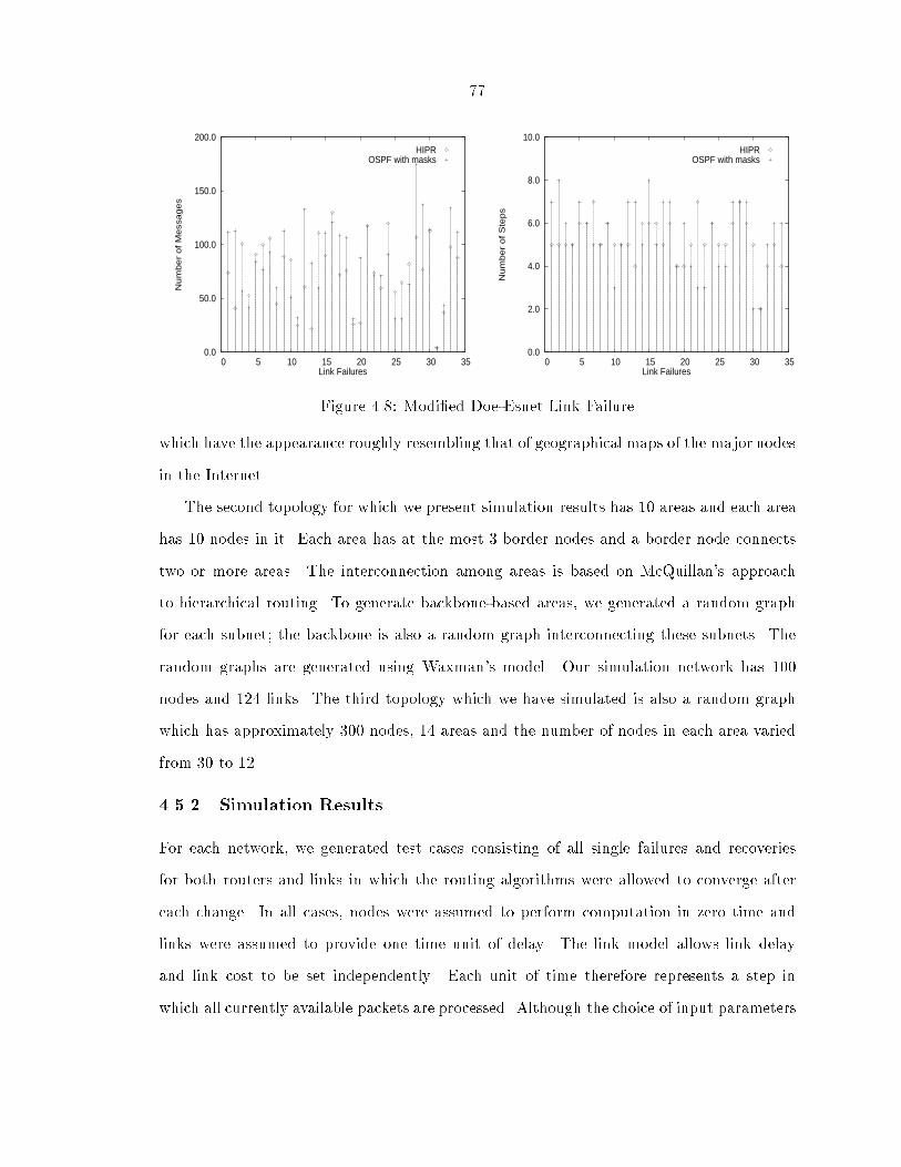
77
0.0
50.0
100.0
150.0
200.0
0 5 10 15 20 25 30 35
Nu
mb
er
of
Me
ssa
ge
s
Link Failures
HIPROSPF with masks
0.0
2.0
4.0
6.0
8.0
10.0
0 5 10 15 20 25 30 35
Nu
mb
er
of
Ste
ps
Link Failures
HIPROSPF with masks
Figure 4.8: Modi�ed Doe-Esnet Link Failure
which have the appearance roughly resembling that of geographical maps of the major nodes
in the Internet.
The second topology for which we present simulation results has 10 areas and each area
has 10 nodes in it. Each area has at the most 3 border nodes and a border node connects
two or more areas. The interconnection among areas is based on McQuillan's approach
to hierarchical routing. To generate backbone-based areas, we generated a random graph
for each subnet; the backbone is also a random graph interconnecting these subnets. The
random graphs are generated using Waxman's model. Our simulation network has 100
nodes and 124 links. The third topology which we have simulated is also a random graph
which has approximately 300 nodes, 14 areas and the number of nodes in each area varied
from 30 to 12.
4.5.2 Simulation Results
For each network, we generated test cases consisting of all single failures and recoveries
for both routers and links in which the routing algorithms were allowed to converge after
each change. In all cases, nodes were assumed to perform computation in zero time and
links were assumed to provide one time unit of delay. The link model allows link delay
and link cost to be set independently. Each unit of time therefore represents a step in
which all currently available packets are processed. Although the choice of input parameters

78
0.0
50.0
100.0
150.0
200.0
0 5 10 15 20 25 30 35
Nu
mb
er
of
Me
ssa
ge
s
Link Recoveries
HIPROSPF with masks
0.0
2.0
4.0
6.0
8.0
10.0
0 5 10 15 20 25 30 35
Nu
mb
er
of
Ste
ps
Link Recoveries
HIPROSPF with masks
Figure 4.9: Modi�ed Doe-Esnet Link Recovery
0.0
200.0
400.0
600.0
800.0
1000.0
0 5 10 15 20
Nu
mb
er
of
Me
ssa
ge
s
Node Failures
HIPROSPF with masks
0.0
5.0
10.0
15.0
20.0
0 5 10 15 20
Nu
mb
er
of
Ste
ps
Node Failures
HIPROSPF with masks
Figure 4.10: Modi�ed Doe-Esnet Node Failure
0.0
50.0
100.0
150.0
200.0
250.0
300.0
350.0
0 5 10 15 20
Nu
mb
er
of
Me
ssa
ge
s
Node Recoveries
HIPROSPF with masks
2.0
4.0
6.0
8.0
10.0
12.0
0 5 10 15 20
Nu
mb
er
of
Ste
ps
Node Recoveries
HIPROSPF with masks
Figure 4.11: Modi�ed Doe-Esnet Node Recovery

79
0.0
2.0
4.0
6.0
8.0
10.0
12.0
Nu
mb
er
of
Ste
ps
Node Failures Link Failures
HIPR
OSPF
HIPR
OSPF
0.0
2.0
4.0
6.0
8.0
10.0
Nu
mb
er
of
Ste
ps
Node Recoveries Link Recoveries
HIPR
OSPF
HIPR
OSPF
Figure 4.12: Modi�ed Doe-Esnet: Average Duration
0.0
50.0
100.0
150.0
200.0
250.0
300.0
350.0
Nu
mb
er
of
Me
ssa
ge
s
Node Failures Link Failures
HIPR
OSPF
HIPR OSPF
0.0
50.0
100.0
150.0
200.0
250.0
Nu
mb
er
of
Me
ssa
ge
s
Node Recoveries Link Recoveries
HIPR
OSPF
HIPR
OSPF
Figure 4.13: Modi�ed Doe-Esnet: Average Number of Messages
100.0
1000.0
10000.0
Nu
mb
er
of
Op
era
tion
s
Node Failures Link Failures
HIPR
OSPF
HIPR
OSPF
100.0
1000.0
10000.0
Nu
mb
er
of
Op
era
tion
s
Node Recoveries Link Recoveries
HIPR
OSPF
HIPR
OSPF
Figure 4.14: Modi�ed Doe-Esnet: Average Number of Operations
causes the simulation to proceed synchronously, the node model treats each incoming packet

80
0.0
5.0
10.0
15.0
20.0
Nu
mb
er
of
Ste
ps
Node Failures Link Failures
HIPR
OSPF
HIPR
OSPF
0.0
2.0
4.0
6.0
8.0
10.0
12.0
14.0
Nu
mb
er
of
Ste
ps
Node Recoveries Link Recoveries
HIPR
OSPF
HIPR
OSPF
Figure 4.15: Random Graph (Topology 2): Average Duration
asynchronously. Each input event is processed independently of other events received during
the same simulation step.
The average of the measured parameters is taken over all resource failures and recoveries.
The algorithm was allowed to converge after each such change. Because of the distribution
of values, both the mean and the standard deviation of the distribution are given. There is
no sampling error for the results because all possible cases are covered.
The graphs in Figures 4.8 and 4.9 depict the number of messages exchanged and the
number of steps required before each algorithm converges for every link failing and recover-
ing in the modi�ed Doe-Esnet topology. Similar graphs for every node failing and recovering
in modi�ed Doe-Esnet are given in Figures 4.10 and 4.11 respectively. All topology changes
are performed one at a time and the algorithms were allowed to converge before the next
resource change. The ordinates of the graphs represents the identi�ers of the links (Fig-
ures 4.8 and 4.9) and nodes (Figures 4.10 and 4.11). The data points show the the number
of messages exchanged after each resource change (graphs on the left hand side) and the
number of steps needed for convergence (graphs on the right hand side) in each of these
�gures.
The graphs in Figures 4.12{4.14 show the average number of steps taken, average number
of messages exchanged and the average number of operations performed for HIPR and OSPF
before each algorithm converges in the case of modi�ed Doe-Esnet topology. The error-bars

81
0.0
50.0
100.0
150.0
200.0
250.0
300.0
350.0
400.0
Nu
mb
er
of
Me
ssa
ge
s
Node Failures Link Failures
HIPR
OSPF
HIPR
OSPF
0.0
20.0
40.0
60.0
80.0
100.0
120.0
Nu
mb
er
of
Me
ssa
ge
s
Node Recoveries Link Recoveries
HIPR
OSPF
HIPR
OSPF
Figure 4.16: Random Graph (Topology 2): Average Number of Messages
10.0
100.0
1000.0
10000.0
Nu
mb
er
of
Op
era
tion
s
Node Failures Link Failures
HIPR
OSPF
HIPR
OSPF
100.0
1000.0
10000.0
Nu
mb
er
of
Op
era
tion
s
Node Recoveries Link Recoveries
HIPR
OSPF
HIPR
OSPF
Figure 4.17: Random Graph (Topology 2): Average Number of Operations
in the graphs indicate the standard deviation of each of the mean values. Similar graphs
for the random topology are shown in Figures 4.15{4.17 for Topology 2 and in Figures
4.18{4.20 for Topology 3 respectively.
HIPR outperforms OSPF in all cases considered. While the number of steps taken by
HIPR to converge after a resource failure is comparable to OSPF, the number of steps
taken to converge after a resource recovery is signi�cantly better than that of OSPF. For
the modi�ed doe-esnet topology, the number of messages exchanged after node failure and
recovery in case of OSPF is twice that of HIPR. The number of operations required by
OSPF is an order of magnitude greater than HIPR. HIPR needs 300 operations where
OSPF needs about 5000 operations. For Topologies 2 and 3 also the number of messages

82
0.0
5.0
10.0
15.0
20.0
Nu
mb
er
of
Ste
ps
Node Failures Link Failures
HIPR
OSPF
HIPR
OSPF
0.0
2.0
4.0
6.0
8.0
10.0
12.0
14.0
Nu
mb
er
of
Ste
ps
Node Recoveries Link Recoveries
HIPR
OSPF
HIPR
OSPF
Figure 4.18: Random Graph (Topology 3): Average Duration
0.0
50.0
100.0
150.0
200.0
250.0
300.0
350.0
400.0
450.0
Nu
mb
er
of
Me
ssa
ge
s
Node Failures Link Failures
HIPR
OSPF
HIPR
OSPF
0.0
50.0
100.0
150.0
200.0
Nu
mb
er
of
Me
ssa
ge
s
Node Recoveries Link Recoveries
HIPR
OSPF
HIPR
OSPF
Figure 4.19: Random Graph (Topology 3): Average Number of Messages
exchanged after a resource failure in OSPF is at least twice that of HIPR and the number
of messages exchanged after a resource recovery is always greater than HIPR. The number
of operations in OSPF is an order of magnitude greater than that of HIPR.
This emphirical results illustrates the performance advantage provided by the distributed
implementation of Dijkstra's shortest path algorithm in HIPR. It is clear that HIPR has
better average performance compared to OSPF in all cases.
4.6 Summary
HIPR, the �rst hierarchical routing algorithm based on the maintenance and exchange of
hierarchical routing trees, has been presented. The main idea of HIPR is to provide a
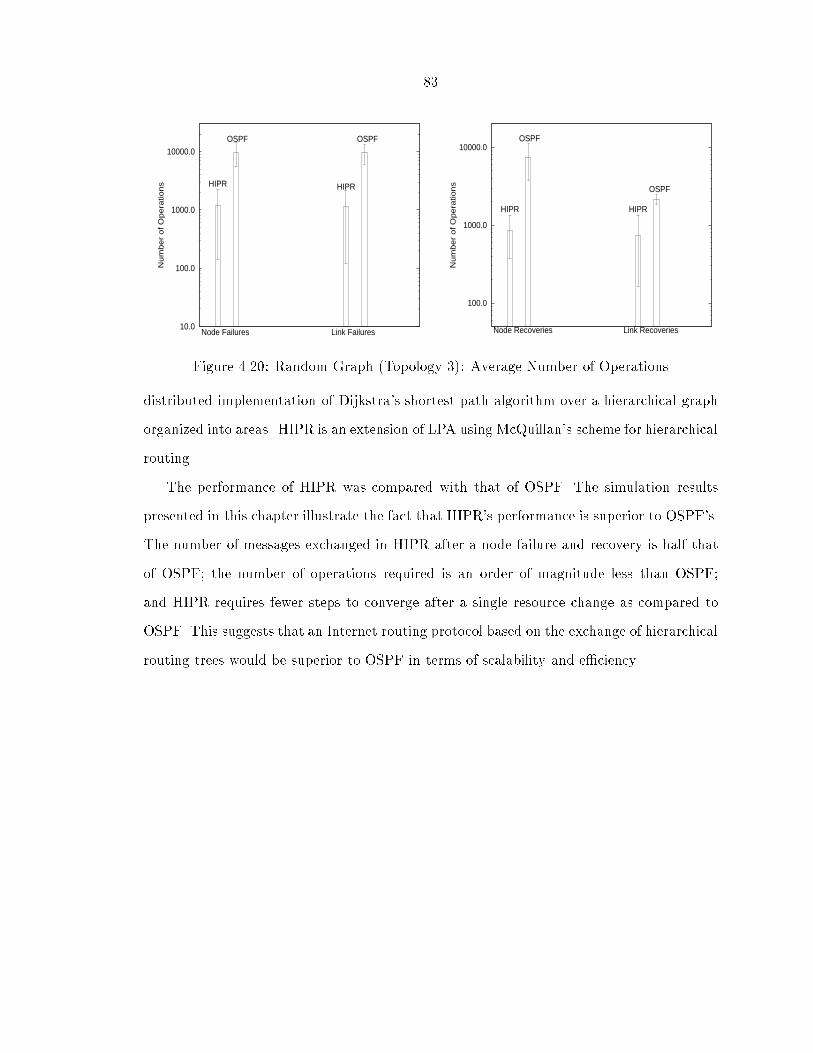
83
10.0
100.0
1000.0
10000.0N
um
be
r o
f O
pe
ratio
ns
Node Failures Link Failures
HIPR
OSPF
HIPR
OSPF
100.0
1000.0
10000.0
Nu
mb
er
of
Op
era
tion
s
Node Recoveries Link Recoveries
HIPR
OSPF
HIPR
OSPF
Figure 4.20: Random Graph (Topology 3): Average Number of Operations
distributed implementation of Dijkstra's shortest path algorithm over a hierarchical graph
organized into areas. HIPR is an extension of LPA using McQuillan's scheme for hierarchical
routing.
The performance of HIPR was compared with that of OSPF. The simulation results
presented in this chapter illustrate the fact that HIPR's performance is superior to OSPF's.
The number of messages exchanged in HIPR after a node failure and recovery is half that
of OSPF; the number of operations required is an order of magnitude less than OSPF;
and HIPR requires fewer steps to converge after a single resource change as compared to
OSPF. This suggests that an Internet routing protocol based on the exchange of hierarchical
routing trees would be superior to OSPF in terms of scalability and e�ciency.

84
Chapter 5
Routing in Wireless Networks
Today's Internet technology has been extremely successful in linking huge number of com-
puters and users. However, this technology is oriented towards computer interconnection in
relatively stable operational environments, which cannot adequately support many of the
emerging uses.
Wireless communication is the next step in the evolution of data networking. Wire-
less networks have the potential to replace the conventional wired networks where cabling
proves impractical. This technology is intended to provide pervasive communication ser-
vices to individuals regardless of their location. In a wireless data-network, workstations are
networked using radio transmissions to accommodate mobility requirements. This requires
e�cient information exchange among the mobile nodes/routers. In this chapter we present
an e�cient routing protocol for wireless packet radio networks, which takes into account
the requirements of a wireless data network. This protocol, which we call Wireless Routing
Protocol (WRP), is based on path-�nding algorithm (PFA) described in Chapter 3.
Routing protocols used in multihop packet-radio networks implemented in the past [Bea89,
Bey90, LNT87] are based on shortest-path routing algorithms that have been typically based
on the distributed Bellman-Ford algorithm (DBF) [BG92]. According to DBF, a routing
node knows the length of the shortest path from each neighbor to every network destination
and this information is used to compute the shortest path and the successor in the path
to each destination. An update message contains a vector of one or more entries, each of
which speci�es as a minimum, the distance to a given destination. A major performance
85
problem with DBF is that it takes a very long time to update the routing tables of network
nodes after network partitions, node failures, or increase in network congestion as it has
no inherent mechanism to determine when a network node should stop incrementing its
distance to a given destination (counting-to-in�nity problem).
As mentioned earlier in Chapter 2, counting-to-in�nity problem can be overcome in three
ways in the existing Internet routing protocols. However, there are signi�cant di�erences
between wireless networks and wired internets in which Internet routing protocols are used.
A wired Internet has relatively high bandwidth and topology that changes infrequently;
in contrast, wireless networks have mobile nodes and have limited bandwidth for network
control. Accordingly, ooding, multihop internodal synchronization and the speci�cation of
complete path information would incur too much overhead in a multihop packet radio net-
work with a dynamic topology. On the other hand, the routing protocols based on DBF or
modi�cations of DBF would take a long time to converge and the frequent topology changes
in a wireless network with mobile nodes make the looping problem of DBF unacceptable.
Therefore, there is a need for a new routing protocol, which is devoid of all these drawbacks.
In the recent past, a number of e�orts have been made to address the limitation of DBF
and topology broadcast in mobile wireless networks. One such e�ort is the DSDV proto-
col [PB94]. In this protocol, each mobile host, which is a specialized router, periodically
advertises its view of the interconnection topology to other mobile hosts within the network
to maintain an up to date network state information. Unfortunately, in DSDV a node has
to wait until it receives the next update message originating from the destination in order
to update its distance-table entry for that destination. This implicit destination-centered
synchronization su�ers from the same latency problems as DUAL (and similar algorithms
based on explicit synchronization). DSDV uses both periodic and triggered updates for
updating routing information; also, DSDV oods the sequence numbers originated by each
destination, which could cause excessive communication overhead.
A distributed routing algorithm for mobile wireless networks based on di�using compu-
tations has been proposed by Corson and Ephremides [CE95]. This protocol relies on the
86
exchange of short control packets forming a query-reply process. It also has the ability to
maintain multiple paths to a given destination. This is a destination-oriented protocol in
which separate versions of the algorithm run independently for each destination. Routing
is source-initiated, which means that routes are maintained by those sources that actually
desire routes. Even though this algorithm provides multiple paths to a destination, because
of the query-based synchronization approach to achieve loop-free paths, the communication
complexity could be high.
Path-�nding algorithms are an attractive approach for wireless networks, because they
eliminate counting-to-in�nity problem. As seen in Chapter 3, they converge faster than
the state of the art routing algorithms. In the remaining of this chapter we describe a
wireless routing protocol (WRP) based on PFA illustrating the key aspects of the protocol's
operation and present some performance results.
5.1 Wireless Routing Protocol
5.1.1 Overview
WRP is designed to run on top of the medium-access control protocol of a wireless net-
work. Update messages may be lost or corrupted due to changes in radio connectivity or
jamming. Reliable transmission of update messages is implemented by means of retrans-
missions. After receiving an update message free of errors, a node is required to send a
positive acknowledgment (ACK) indicating that it has a good radio connectivity and has
processed the update message. Because of the broadcast nature of the radio channel, a node
can send a single update message to inform all its neighbors about changes in its routing
table; however, each such neighbor sends an ACK to only the originator node.
In addition to ACKs, the connectivity can also be ascertained with the receipt of any
message from a neighbor (which need not be an update message). To ensure that connec-
tivity with a neighbor still exists when there are no recent transmissions of routing table
updates or ACKs, periodic update messages without any routing table changes (null update

87
messages) are sent to the neighbors. These messages are also known as Hellomessages. The
time interval between two such null update messages is the HelloInterval.
If a node does not receive any message from a neighbor for a speci�ed amount of time
(e.g., three or four times the HelloInterval known as the RouterDeadInterval), the node will
assume that connectivity with that neighbor is lost.
5.1.2 Information Maintained at Each Node
For the purpose of routing, each node maintains a distance table, a routing table, a link-cost
table and a message retransmission list.
The distance table of node i is a matrix containing, for each destination j and each
neighbor of i (say k), the distance to j (Dijk) and the predecessor (pijk) reported by k.
The routing table of a node i is a vector with an entry for each known destination j
which speci�es:
� The destination identi�er (j)
� The distance to the destination (Dij)
� The predecessor of the chosen shortest path to j (pij)
� The successor of the chosen shortest path to j (sij)
� A marker (tagij) used to update the routing table entries; it speci�es whether the entry
corresponds to a simple path (tagij = correct), a loop (tagij = error) or a destination
that has not been marked (tagij = null).
The link-cost table of node i lists the cost of relaying information through each neighbor
k, and the number of periodic update periods that have elapsed since node i received any
error-free messages from k.
The cost of a failed link is considered to be in�nity. The way in which costs are assigned
to links is beyond the scope of this speci�cation. As an example, the cost of a link could
simply be 1 re ecting the hop count, or the addition of the latency over the link plus some
constant bias. The cost of the link from i to k (i; k) is denoted by lik.

88
Procedure Init1when router i initializes itselfdo begin
set a link state table with costs of adjacent links;
N i; Ni x j lix < 1;for each (x 2 Ni)do begin
Ni N [ x; tagix null;
six null; pix null; Dix 1end
Dii 0; si
i null; pi
i null; tagi
i correct
for each j 2 N call Init2(x; j)for each (n 2 Ni) do add (0; i; 0; i) to LISTi(n)x retransmission time; y hello count;z retransmission count;call Send
end
Procedure Init2(x; j)begin
Dijx 1; pi
jx null; si
jx null; seqnoi
jx 0
end
Procedure Sendbegin
for each (n 2 Ni)do begin
if (LISTi(n) is not empty)then send messages with LISTi(n) to nempty LISTi(n)
endend
Procedure Messagewhen router i receives a message on link (i; k)begin
if (k 62 Ni) dobeginNi Ni [ k;
lik cost of new link;
if (k 62 N) begin
N N [ k; tagik null;
Dik 1; pi
k null; si
k null;
for each x 2 Ni do call Init2(x; k)end
for each (i; k; lik) do
send update(0; k; Dik; pik)
end
reset HelloTimer;
for each entry (ukj; j;RDk
j; rpk
j) j i 6= j
do beginif (j 62 N)then begin
if (RDkj=1) then delete entry
else beginN N [ j;for each entry x 2 Ni call Init2(x; j)
tagij null; call DT
endendelse begin
tagij null;
endend
for each entry (ukj; j;RDk
j; rpk
j) left j i 6= j
do case of ukj
0: call Update(j; k)1: call ACK(j; k)
endcall Send
end
Procedure Create RList(seqno)beginseqno seqno + 1; NeighborSet Nibitmap[] 0; RetransmissionTimer x
add updates to RListend
Procedure Delete RList(seqno)begin
set bitmap[seqno] 1; delete 1for all n 2 Ni begin
if (bitmap[seqno] = 0) delete 0;endif (delete = 1) delete RList[seqno] end
Procedure Update RList(seqno)begin
reset RetransmissionTimersend update RList[seqno];
end
Procedure Clean RList (seqno)beginfor all entries in RList
delete RList[seqno];end
Procedure Connectivitywhen HelloTimer expiresbegin
HelloCount[k] HelloCount[k] + 1;if (HelloCount[k] < y) thenreset HelloTimer;
else beginNi Ni � k
call Delete RList(k)
lik 1
tagik null
delete column for k in distance tableupdate routing table
endend
Procedure TimeOut(i; k)when RetransmissionTimer expiresbegin
RetransmissionCounter RetransmissionCounter - 1;if (RetransmissionCounter < z)call Update RList(k)
else beginNi Ni � k
call Delete RList(k)
lik 1
tagik null
delete column for k in distance tableupdate routing table
endend
Procedure DTwhen distance table update has to be donebegin
Dijk li
k+Dk
j; pijk pk
j;
(2) for all neighbors bdo begin
if k is in the path from i to j inthe distance table through neighbor b
then Dijb Di
kb+Dk
j; pijb pk
jend
end
Figure 5.1: Protocol Speci�cation

89
Procedure ACK(n)when router i receives an ACK on link (i; k)begin
call Delete RList(n);RetransmissionCounter z;
end
Procedure Update(i; k)when router i receives an update on link (i; k)begin
send ACK to neighbor kRetransmissionCounter z;RetransmissionTimer x;
(0) beginupdate=0;
RTEMPi �;
DTEMPi;b � for all neighbors b
(1) for each triplet (j;Dkj; pkj) in V k;i; j 6= i do
call procedure DT(3) begin
if there are b and j such that
(Dijb
< Dij) or ((Di
jb> Di
j) and (b = si
j))
then call RT Updateend
(4) begin if (RTEMPi 6= �) thenfor each neighbor b do begin
for each triplet t = (j;Dij; pij) in RTEMPi
do beginif b is not in the path from i to j
then DTEMPi;b DTEMPi;b [ t;end
send DTEMPi;b to neighbor b;end
endend
Procedure RT Updatewhen routing table has to be updatedbegin
�nd minimum of the distance entries DTminif (Di
j sij
= DTmin) then ns sij
else ns b j fb 2 Ni and Dijb
= DTming;
x j;
while (Dix ns = MinfDixb8 b 2 Nig
and Dixns<1 and tagix = null)
do x pix ns;
if (pix ns = i or tagix = correct)
then tagij correct else tagi
j error
if (tagij= correct) then begin
if (Dij6= DTmin or pi
j6= pi
j ns) then begin
seqno seqno + 1;
add (0, j, DTmin , pij ns
; seqno) to LISTi(x) 8x 2 Ni;
call Clean RList(seqno)call Create RList(seqno)
end
Dij DTmin; p
ij pi
j ns; sij ns
endelse begin
if(Dij<1) then begin
seqno seqno + 1;add (0, j, 1, null, seqno) to LISTi(x) 8x 2 Ni ;call Clean RList(seqno)call Create RList(seqno)
end
Dij 1; pi
j null; si
j null
endend
Figure 5.2: Protocol Speci�cation (Cont..)
The message retransmission list (MRL) speci�es one or more retransmission entries,
where the mth entry consists of the following:
� The sequence number of an update message
� A retransmission counter that is decremented every time node i retransmits an update
message
� A ag indicating whether node i has received an ACK from neighbor k to the update
message sent to k (present in the retransmission entry)
� The list of updates sent in the update message
The above information permits node i to know which updates of an update message
(each update message may contain a list of updates) have to be retransmitted when the
timer expires and which neighbors should be requested to acknowledge such retransmission.
Node i retransmits the list of updates in an update message when the retransmission timer

90
of the corresponding entry in the MRL expires. The retransmission counter of a new entry
in the MRL is set equal to a small number (e.g., 3 or 4).
5.1.3 Information Exchanged among Nodes
In WRP, nodes exchange routing-table update messages (which we call \update messages"
for brevity) that propagate only from a node to its neighbors. An update message contains
the following information:
� The identi�er of the sending node.
� A sequence number assigned by the sending node.
� An update list of zero or more updates or ACKs to update messages. An update
entry speci�es a destination, a distance to the destination, and a predecessor to the
destination. An ACK entry speci�es the source and sequence number of the update
message being acknowledged.
� A response list of zero or more nodes that should send an ACK to the update message.
In the event that the message space is not large enough to contain all the updates and
ACKs that a node wants to report, they are sent in multiple update messages. An example
of this event can be the case in which a node identi�es a new neighbor and sends its entire
routing table.
The response list of the update message is used to avoid the situation in which a neighbor
is asked to send multiple ACKs to the same update message, simply because some other
neighbor of the node sending the update did not acknowledge.
The �rst transmission of an update message must ask all neighbors to send an ACK, of
course, and this is accomplished by specifying the \all-neighbors address," which consists
of all 1's.
When the update message reports no updates, the \empty address" is speci�ed; this
address consists of all 0's and instructs the receiving nodes not to send an ACK in return.
This type of update message is used as a \hello message" from a node to allow its neighbors

91
to know that they maintain connectivity, even if no user messages or routing-table updates
are exchanged.
As we explain subsequently, an ACK entry refers to an entire update message, not an
update entry in an update message, in order to conserve bandwidth.
5.1.4 Routing-Table Updating
Figures 5.1 and 5.2 specify important procedures of WRP used to update the routing and
distance tables.
A node can decide to update its routing table after either receiving an update message
from a neighbor, or detecting a change in the status of a link to a neighbor. When a node
i receives an update message from its neighbor k, it processes each update and ACK entry
of the update message in order.
In WRP, a node checks the consistency of predecessor information reported by all its
neighbors each time it processes an event involving a neighbor k. i.e., the distance table
is updated for all entries referring directly to neighbor k and all other entries that refer to
node k indirectly (k is in the path of a destination). In contrast, all previous path-�nding
algorithms [CRKGLA89, Hum91, RF91] check the consistency of the predecessor only for
the neighbor associated with the input event. This unique feature of WRP accounts for its
fast convergence after a single resource failure or recovery as it eliminates more temporary
looping situations than previous path-�nding algorithms.
Processing an Update: To process an update from neighbor k regarding destination j,
the distance and the predecessor entries in the distance table are updated. A ag (tag) is
set to specify that this entry in the table has been changed. A unique feature of WRP is
that node i also determines if the path to destination j through any of its other neighbors
fb 2 Nijb 6= kg includes node k. If the path implied by the predecessor information
reported by node b includes node k, then the distance entry of that path is also updated as

92
Dijb = Di
kb +Dkj and the predecessor is updated as pijb = pkj . Thus, a node can determine
whether or not an update received from k a�ects its other distance and routing table entries.
To update its distance and predecessor for destination j (procedure RT Update), node
i chooses a neighbor p that has reported routing information such that:
� The path from p to j (which is implied by the predecessor information reported by p)
does not include node i
� Dijp � Di
jx for any other neighbor x, and Diyp � Di
yx for any other neighbor x and for
every node y in the path from i to j.
The above means that node i chooses node p as its successor to a destination j if that
neighbor appears to o�er a smallest-cost loop-free path to j on all the intermediate nodes
in the path to j.
When node i sends an update message, it updates its message retransmission list. For
each destination j for whom an update is being reported, node i sets the ack-required ag
for all its neighbors. It also adds an entry in the message-retransmission list containing the
sequence number given to the update message, and starts the retransmission timer for that
entry.
Sending New and Retransmitted Update Messages: Node i sends a new update
message after processing updates from its neighbors or detecting a change in the status of
the link to a neighbor. Whenever node i sends a new update message, it must
� Add an entry in the MRL for the new update message
� Delete the updates in the existing entries of MRL for the updates that are included
in the new update message
� Initialize the retransmission counter of ther new update messages entry in the MRL
to a maximum value.
When the list of updates of a MRL entry is outdated by the transmission of a new
update message, node i erases the old entry from the MRL.

93
When the retransmission timer for a entry m in the MRL expires, node i retransmits
the update message as an update list containing the list of updates of the retransmission
entry, and a response list specifying those neighbors who did not acknowledge the update
message earlier (i.e., every neighbor k for whom aikm = 1). The retransmission counter of
that entry in the MRL is decremented.
Note that, if we do not use the retransmission counter, based on the above retransmission
strategy, there is no limit on the number of times node i would retransmit an update message
to an existing neighbor. However, as we discuss below, node i stops considering node k as
its neighbor after it fails to communicate with it for some �nite amount of time.
Retransmission counter limits the number of times an update can be retransmitted to a
neighbor. Each time an update is retransmitted, the corresponding retransmission counter
is decremented. If an ACK is not received from a neighbor before the retransmission counter
becomes zero, then that neighbor is assumed to be no longer existent.
Processing an ACK: An ACK entry in an update message refers to another update
message, i.e., it acknowledges all the updates included in the update message bearing the
referenced sequence number. Therefore, it is up to the node whose update message is being
acknowledged to ascertain which updates are implied by a received ACK.
To process an ACK from neighbor k, node i scans its MRL for the sequence number
matching the sequence number speci�ed in the ACK received. When a match is found, node
i resets the ack-required ag for neighbor k; if aipm = 0 for entry m and every neighbor p of
node i; the retransmission entry is deleted if all entries of the retransmission entry has been
acknowledged. This scheme obtains short ACKs at the expense of additional processing.
Node i may receive an ACK for an update message whose retransmission entry has been
erased after sending a more recent update message for the same destinations. In that case,
node i simply ignores the ACK.
Handling Topology and Link-Cost Changes: To ensure that nodes know that they
have connectivity even when they do not transmit user messages or routing-table updates
94
for some time, every node must periodically send an update message reporting no changes
(hello messages). Acknowledgments are not required for such update messages, and they
can be very short (e.g., a byte for control information and a byte for the node identi�er,
since the control information can imply that there is no sequence number, update list, or
response list in the message). Alternatively, a node may retransmit an update message if
it is not too long. On initialization, a node transmits a hello message.
Given that short periodic update messages are transmitted by every node, the failure of a
link to a neighbor is detected by the lack of any user or update messages being received from
that neighbor over a period of time equal to a few update-message transmission periods.
Similarly, new links and nodes are detected by means of update messages or user messages.
When node i receives an update or user message from node k and node k is not listed in
its routing table or distance table, it adds the corresponding entry to its distance or routing
table for destination k. An in�nite distance to all destinations through node k is assumed,
with the exception of node k itself and those destinations reported in node k's updates, if
the message received from k was an update message. In addition, node i noti�es node k of
the information in its routing table. This information can be transmitted in one or multiple
update messages that only node k needs to acknowledge.
When a link fails or a link-cost changes, node i recomputes the distances and predeces-
sors to all a�ected destinations, and sends to all its neighbors an update message for all
destinations whose distance or predecessor have changed.
5.2 Correctness of WRP
In this section, we show that the basic routing algorithm used in WRP is correct. The
following assumptions are made on the behavior of links and routers for the working of
WRP.
1. Messages are transmitted reliably. A lower-level protocol is responsible for maintaining
the status of the link.

95
2. Messages are sent by a router over a link only when the link is perceived as being up.
3. A router that is not functional cannot receive or send any messages.
4. All routers are initially down.
5. Update messages received by a router are processed in the order of their arrival
(FIFO).
6. Link lengths are always positive and a failed link has an in�nite length.
7. Time T is de�ned such that between the time interval 0 and T links and routers go
up and down and the cost of the link changes; at time T , links have the same status
at both ends and there are no changes after time T .
For simplicity, the proof assumes that all update messages sent over an operational
link are received correctly. In practice, WRP handles errors by means of retransmissions.
In terms of the correctness proof, the e�ect of retransmissions is that of added delay in
the delivery of an update message to a neighbor, and a link fails when a given number
of retransmissions have been attempted. In essence, this proof is very much similar to
that of the path-�nding algorithm (PFA) on which WRP is based is correct. The proof of
correctness is given in [MGLA96].
WRP's time complexity is O(h) in the worst-case, where h is the height of the routing
tree. Time complexity is de�ned as the largest time that can elapse between the moment T
when the last topology change occurs and the moment at which all the routers have �nal
shortest path to all other routers. Communication complexity is de�ned as the maximum
number of node identities exchanged (messages) after time T before the �nal graph is
reached.
5.3 Simulation Results
We have studied the average-case performance of WRP in a dynamic environment using
Drama. The performance of the basic routing algorithm used in WRP has been compared

96
with that of DUAL and ILS. In order to simulate mobility, the connectivity of a mobile
node is said to be lost when a node does not hear from a mobile node for a certain period of
time. The connectivity with a node will be reestablished when a node hears from a mobile
node again. Mobility is modeled as an arbitrary set of failures and recoveries of a mobile
node at random points in time. All simulations are done assuming unit propagation time
and zero packet processing time at each node. If a mobile node fails when the packets are
in transit, the packets are assumed to get dropped.
Our goal is to compare the performance of WRP against the performance of routing
protocols based on DBF, DUAL, and ILS. To reduce the complexity of the simulation, we
have eliminated those features of the protocols that were common to all; these features
concern the reliable transmission of updates over unreliable links, and the identi�cation of
neighbors. Accordingly, our simulation assumed that, for any of the protocols simulated,
any update message sent over an operational link is received correctly, and that a node
always receives enough user messages to know that it continues to have connectivity with a
neighbor. According to these assumptions, there is no need to account for acknowledgments,
retransmissions of updates, or periodic transmissions of update messages.
However, our intent in running the simulations was to obtain insight on the comparative
overhead of di�erent protocols that necessarily require the transmission of acknowledgments
to update messages. We approached this problem in the following manner: In a wireless
packet radio network, the same update messages sent by a node is received by all its neigh-
bors, i.e., each update message is broadcast to a node's neighbors. However, to guarantee
the reliable transmission of updates, each neighbor must send an acknowledgment to the
sender of the update. Therefore, under the assumption that no errors or collisions occur in
the network channel, counting the number of acknowledgments received for a single update
broadcast to all neighbors is much the same as counting the number of updates sent by
a node to its neighbors on a point-to-point basis and with no acknowledgments|the two
counts di�er only by one. Accordingly, we simulated the routing protocols' operation in
a wireless network using the same point-to-point links typical of wireline networks. The

97
message count obtained from the simulation runs is not the exact number of updates and ac-
knowledgments sent by each protocol, but accurately re ects the relative di�erences among
protocols.
The resulting simpli�ed version of WRP we simulated is simply the path �nding algo-
rithm (PFA), and is the same basic algorithm �rst described in [MGLA94]. Similarly, ILS,
DBF, and DUAL correspond to the ideal case of the best protocols that could be designed
based on these algorithms.
The simulations were run on several network topologies such as Los-Nettos, Nsfnet and
Arpanet. We chose these topologies to compare the performance of routing algorithms for
well-known cases given that we cannot sample a large enough number of networks to make
statistically justi�able statements about how an algorithm scales with network parameters.
The Los-Nettos topology has 11 nodes, a diameter of 4 hops, and each node has at most
four neighbors. The Nsfnet topology has 13 nodes, a diameter of 4 hops, and each node has
at most 4 neighbors. The Arpanet topology has 57 nodes, a diameter of 8 hops, and each
node has a maximum of four neighbors.
For the routing algorithms under consideration, there is only one shortest path between
a source and a destination pair and we do not consider null paths from a node to itself. Data
are collected for a large number of topology changes to determine statistical distribution.
The statistics has been collected after each failure and recovery of a link. To obtain the
average �gures, we make each link (or node) in the network fail and count the number of
steps and messages required for each algorithm to converge. Then the same link (node)
is made to recover and the process is repeated. The average is taken over all failures and
recoveries. Again, this message count is not exact, but the relative di�erence from one
protocol to another is accurate.
5.3.1 Dynamics with Mobile Nodes
We modeled mobility in the simulation by making the links fail and come back up arbitrarily
at random times. The network is assumed to be fully connected with potential links. At

98
startup, the topology is initialized to some well known topology, such as Los-Nettos, Nsfnet
or Arpanet. After initialization, to simulate the movement of a node, a node is assumed
to have failed at its previous location and reappear in its new location. Node failure is
simulated as all the links associated with that node going down at the same time. The
gradual movement of a node from one location to another is simulated by means of link
failures and additions. When a link fails, it can be assumed that a node is no longer in the
neighborhood of its previous neighbor. The addition of a new link is viewed as a movement
of a node wherein, a node reappears in the new neighborhood.
The links are chosen at random from the set of all the existing links in the fully connected
network. Selecting any particular link is equally likely. The probability of a link failing or
recovering is also equally likely. We also have imposed an additional condition in our
simulations that a node at any given time cannot have more than x neighbors. Here, x
indicates the degree of the node. This condition is imposed in order to make sure that
all the links pertaining to one node alone will not be active. This helps in simulating
the mobility more closely. This, of course, is only an approximation of the more gradual
topology changes that would be experienced in a real mobile network.
The average number of messages and the average message length for each of these
algorithms are obtained by varying the interarrival time between two events (Figures 5.3{
5.5). An event can be either a link failure or a link recovery. For the purpose of event
generation, we consider a fully connected topology and start o� with a given initial topology.
Since any random link can fail or recover at any time, our model simulates mobility closely.
The above results indicate that the routing algorithm of WRP outperforms all other
algorithms which we have simulated, namely, DBF, DUAL and ILS. We were not able to
simulate ILS for the Arpanet topology due to limited resources. The statistics about the
average number of messages and the average message length have been collected for all
the above mentioned topologies for all the four algorithms by varying the interarrival time
between events (failures and recoveries).

99
1.0
10.0
100.0
1.0 10.0 100.0 1000.0 10000.0
AV
ER
AG
E N
UM
BE
R O
F M
ES
SA
GE
S
INTERARRIVAL TIME
PFADBF
DUALILS
0.10
1.00
10.00
1.0 10.0 100.0 1000.0 10000.0
AV
ER
AG
E M
ES
SA
GE
LE
NG
TH
INTERARRIVAL TIME
PFADBF
DUALILS
Figure 5.3: Los-Nettos
10.0
100.0
1.0 10.0 100.0 1000.0 10000.0
AV
ER
AG
E N
UM
BE
R O
F M
ES
SA
GE
S
INTERARRIVAL TIME
PFADBF
DUALILS
0.10
1.00
10.00
1.0 10.0 100.0 1000.0 10000.0
AV
ER
AG
E M
ES
SA
GE
LE
NG
TH
INTERARRIVAL TIME
PFADBF
DUALILS
Figure 5.4: Nsfnet100.0
1.0 10.0 100.0 1000.0 10000.0
AV
ER
AG
E N
UM
BE
R O
F M
ES
SA
GE
S
INTERARRIVAL TIME
PFADBF
DUAL
1.00
1.0 10.0 100.0 1000.0 10000.0
AV
ER
AG
E M
ES
SA
GE
LE
NG
TH
INTERARRIVAL TIME
PFADBF
DUAL
Figure 5.5: ARPANET
In all cases, the average number of messages for DBF and DUAL are more than that
of WRP. This results from DBF's counting-to-in�nity problem and DUAL's use of an

100
interneighbor coordination mechanism to achieve loop-freedom and this synchronization
mechanism spans the entire diameter of the network. ILS sends maximum number of mes-
sages since the complete topology information has to be exchanged between neighbors every
time the topology changes.
The average length of each message is the highest in DUAL as compared to all other
algorithms. The average message length in case of ILS is almost constant since it always
sends the complete topology information. Even though we do not have simulation results
for ILS in case of Arpanet topology, we can extrapolate the results from the other two
network topologies and can expect similar behavior for Arpanet topology also.
5.4 Implementation Status
We have completed an initial implementation of the wireless routing protocol under the
BSD version of the UNIX operation system [Ana96]. This implementation contains all fea-
tures of the basic WRP, and we are currently considering additions to the implementations
to support subnetting. Our implementation includes all functions of the basic routing al-
gorithm, the hello protocol, which is used to maintain neighbor discovery information and
the reliable exchange of messages (which includes ACKs).
The implementation is mainly done in the user space and the kernel routing tables are
updated as and when required. We are also considering the implementation of WRP based
on the implementation of some of the existing routing daemons of UNIX such as routed and
gated.
5.4.1 Optimization
In order to reduce the routing control messages in the protocol and thus to minimize the
protocol overhead, we limit the number of times a Hello packet has to be sent to the
neighbors. Any packet received from a neighbor can be treated as an implicit Hello and the
hello timer will be reset. Only when there is no tra�c in the network, an explicit Hello will
be sent to the neighbors. This reduces the number of control messages in the network.

101
In order to reduce the number of acknowledgments exchanged for each update, we use
piggy-backed acknowledgments. After an update is received and before an ACK is sent in
response to that update, if the node has any updates to be sent to the neighbor for which
it has to send the ACKs, these ACKs will be piggy-backed with the updates.
5.5 Summary
In this chapter, we have described a wireless routing protocol, WRP, which is based on
path-�nding algorithm. A mechanism has been proposed for the reliable exchange of update
messages as part of WRP. The basic algorithm used in WRP has been proved to be correct
and WRP's complexity has been analyzed. The performance of the routing algorithm in
WRP has been compared with that of an ideal topology broadcast algorithm (ILS), DUAL
and DBF for highly dynamic environment through simulations. The simulation results
show that WRP provides about 50% improvement in the convergence time as compared to
DUAL. The results indicate that WRP is an excellent alternative for routing in wireless
networks.

102
Chapter 6
Congestion-Oriented Routing
The previous chapters described routing algorithms and protocols for various network en-
vironments such as hierarchical networks and wireless networks. Using e�cient routing
algorithms we get small average packet delays but, the network might be able to accept
more tra�c if ow control is associated with routing. On the other hand, e�cient ow con-
trol algorithm alone rejects excessive o�ered load that would necessarily increase the packet
delays by saturating network resources. This can possibly be avoided by rerouting packets
through non-congested links. Therefore, it is clear that routing and congestion-control are
very much interrelated.
In this chapter, we present a congestion-oriented multipath routing algorithm in which
we combine congestion-control with routing and present an integrated solution based on
credits. Our objective is to provide certain level of performance guarantees in a connec-
tionless network. This we do by de�ning a two-tier architecture where connection oriented
sessions are mapped on to connectionless ows thereby supporting multiple QoS levels. To
the end user, this architecture looks very much similar to a connection-oriented architecture
through which several levels of performance guarantees can be requested. We �rst describe
the connectionless model and then present the two-tier model.
6.1 Prior Work
One of the drawbacks of the existing Internet routing protocols is that their main routing
mechanisms (route computation and packet forwarding) are poorly integrated with conges-

103
tion control mechanisms. More speci�cally, today's Internet routing is based on single-path
routing algorithms. Even in theory, a routing protocol based on single-path routing is ill
suited to cope with congestion. The only thing a single path routing protocol can do to
react to congestion is to change the route used to reach a destination. However, as has been
documented in [Ber82], allowing a single-path routing algorithm to react to congestion can
lead to unstable oscillatory behavior.
Datagram based networks carry tra�c that spans a fairly wide range of rates, but
their performance is guaranteed on a best e�ort basis only. Recently, quality of service
(QoS) has become a very important issue. The newer Internet routing protocols such as
IPv6 [DH96] have mechanisms to support di�erent service qualities. This implies that
just best-e�ort service alone does not su�ce for datagram networks for future applications.
Also, current routing protocols react to congestion after the network resources have been
wasted i.e., a source reacts to congestion only after it receives a congestion indication from
the congested resource in the data path before the source can regulate the rate at which
it inputs data into the network. Furthermore, for a connectionless service, any datagram
o�ered to the network is accepted. It is up to the transport protocol to react to congestion
after network resources are already being wasted. This requires a congestion control scheme
which is responsive to the changes in the available bandwidth and e�ciently uses the unused
bandwidth. The bandwidth must be available on a timely basis allowing application to
almost instantaneously use the available bandwidth while maintaining low packet losses.
Hop-by-hop credit-based schemes have a potential for the desired responsiveness [KTA94].
The performance of these schemes is independent of the input tra�c pattern. These schemes
can be used to fairly share the network bandwidth among competing ows. Also, when there
is bandwidth contention, each ow obtains a fair share of the bandwidth.
Our work was motivated by our conjecture that architectural elements similar to those
used in a connection-oriented architecture to allow the network to enforce performance
guarantees can be used in a connectionless architecture to integrate routing with congestion
control, and to provide some delay bounds for the delivery of those datagrams that are

104
accepted in the network. We propose a new framework and protocol for dynamic multipath
routing in packet-switched networks that attempts to prevent over-utilization of network
resources and hence congestion. Packets are individually routed towards their destinations
on a hop-by-hop basis. A packet intended for a given destination is allowed to enter the
network if and only if there is at least one path of routers with enough resources to ensure
its delivery within a �nite time. In contrast to existing connectionless routing schemes, once
a packet is accepted into the network, it is delivered to its destination, unless a resource
failure prevents it. Each router reserves bu�er space for each destination, rather than for
each source-destination session as it is customary in a connection-oriented architecture, and
forwards a received packet along one of multiple loop-free paths towards the destination.
The bu�er space and available paths for each destination are updated to adapt to congestion
and the dynamic state of the network.
Our framework is based on three main architectural elements namely:
� tra�c shaping by means of destination-oriented permit buckets
� tra�c separation and scheduling on a per destination basis
� maintenance of dynamic multiple loop-free paths to reduce the delay from source to
destination.
Permit buckets consist of permits or tokens fed by periodic updates of credits. To
schedule packet transmission, we assume a packet-by-packet generalized processor sharing
(PGPS) server [PG93] at each node. To establish loop-free multipaths, we extend prior
results on loop-free single-path routing algorithms introduced in [GLAM95]. This results in
a congestion-oriented multipath routing architecture that uses a short-term metric based on
hop-by-hop credits to reduce congestion over a given link, and a long-term metric based on
end-to-end path delay to reduce delay from source to destination. The main contribution of
this work is to illustrate the provision of performance guarantees in a connectionless routing
architecture.
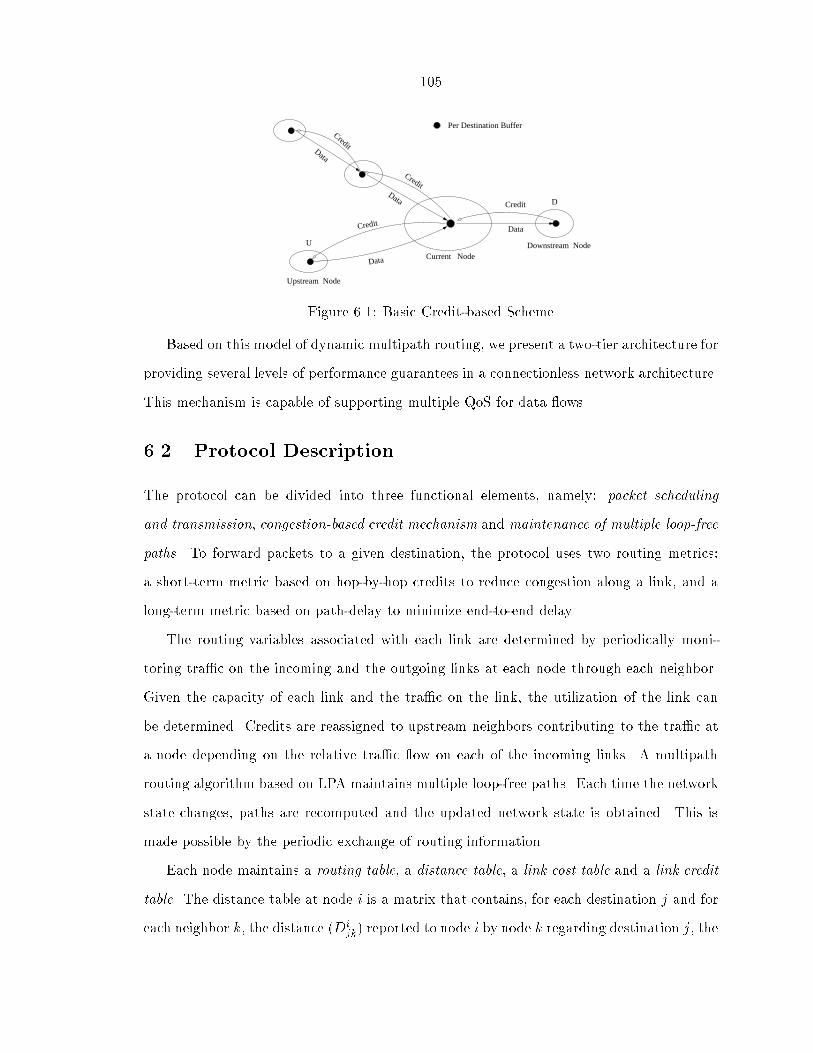
105
DCredit
Data
Per Destination Buffer
Current Node
Upstream Node
Downstream Node
Credit
Data
Data
Data
Credit
Credit
U
Figure 6.1: Basic Credit-based Scheme
Based on this model of dynamic multipath routing, we present a two-tier architecture for
providing several levels of performance guarantees in a connectionless network architecture.
This mechanism is capable of supporting multiple QoS for data ows.
6.2 Protocol Description
The protocol can be divided into three functional elements, namely: packet scheduling
and transmission, congestion-based credit mechanism and maintenance of multiple loop-free
paths. To forward packets to a given destination, the protocol uses two routing metrics:
a short-term metric based on hop-by-hop credits to reduce congestion along a link, and a
long-term metric based on path-delay to minimize end-to-end delay.
The routing variables associated with each link are determined by periodically moni-
toring tra�c on the incoming and the outgoing links at each node through each neighbor.
Given the capacity of each link and the tra�c on the link, the utilization of the link can
be determined. Credits are reassigned to upstream neighbors contributing to the tra�c at
a node depending on the relative tra�c ow on each of the incoming links. A multipath
routing algorithm based on LPA maintains multiple loop-free paths. Each time the network
state changes, paths are recomputed and the updated network state is obtained. This is
made possible by the periodic exchange of routing information.
Each node maintains a routing table, a distance table, a link cost table and a link credit
table. The distance table at node i is a matrix that contains, for each destination j and for
each neighbor k, the distance (Dijk) reported to node i by node k regarding destination j, the
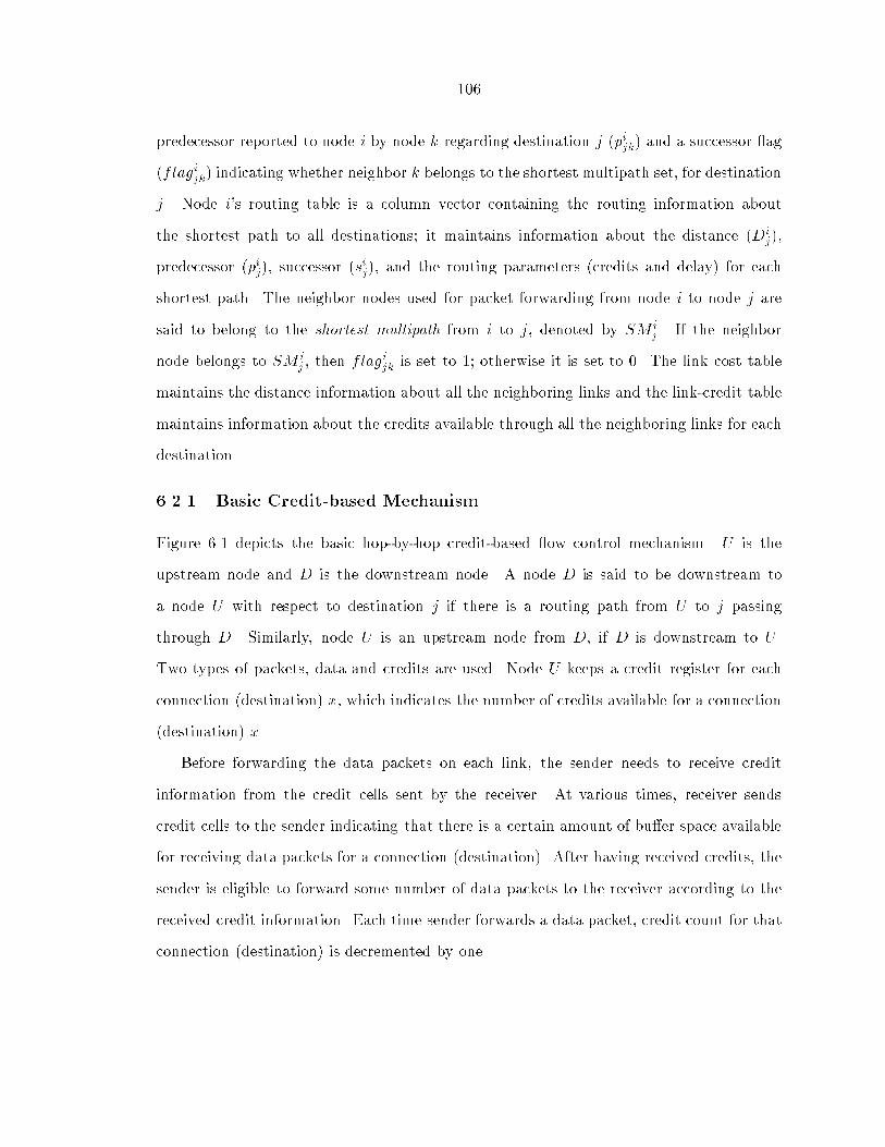
106
predecessor reported to node i by node k regarding destination j (pijk) and a successor ag
(flagijk) indicating whether neighbor k belongs to the shortest multipath set, for destination
j. Node i's routing table is a column vector containing the routing information about
the shortest path to all destinations; it maintains information about the distance (Dij),
predecessor (pij), successor (sij), and the routing parameters (credits and delay) for each
shortest path. The neighbor nodes used for packet forwarding from node i to node j are
said to belong to the shortest multipath from i to j, denoted by SM ij . If the neighbor
node belongs to SM ij , then flagijk is set to 1; otherwise it is set to 0. The link cost table
maintains the distance information about all the neighboring links and the link-credit table
maintains information about the credits available through all the neighboring links for each
destination.
6.2.1 Basic Credit-based Mechanism
Figure 6.1 depicts the basic hop-by-hop credit-based ow control mechanism. U is the
upstream node and D is the downstream node. A node D is said to be downstream to
a node U with respect to destination j if there is a routing path from U to j passing
through D. Similarly, node U is an upstream node from D, if D is downstream to U .
Two types of packets, data and credits are used. Node U keeps a credit register for each
connection (destination) x, which indicates the number of credits available for a connection
(destination) x.
Before forwarding the data packets on each link, the sender needs to receive credit
information from the credit cells sent by the receiver. At various times, receiver sends
credit cells to the sender indicating that there is a certain amount of bu�er space available
for receiving data packets for a connection (destination). After having received credits, the
sender is eligible to forward some number of data packets to the receiver according to the
received credit information. Each time sender forwards a data packet, credit count for that
connection (destination) is decremented by one.

107
The advantages of credit-based ow control scheme are maximizing network utilization
and controlling congestion.
6.2.2 Message Types
Messages are exchanged among routers for the proper functioning of the protocol. We
classify the messages into six types.
Explicit Credit Requests: When a source becomes active and has some data to be sent
towards a destination it sends an explicit credit request message to the destination of
that ow requesting for credits. Explicit credit requests are associated with sequence
numbers. The state of the source indicating the source which initiated the credit
request and the corresponding sequence number are recorded at the time of request.
(These messages can be viewed analogous to PATH messages in RSVP).
Explicit Credit Response: This message is sent in response to an explicit credit re-
quest message and indicates the credit availability for data transmission and the se-
quence number of the request. The available credits are then distributed among the
sources that requested for credits. (These messages are analogous to RESV messages
of RSVP).
Explicit Teardown: This message is sent to reclaim all the credits assigned to a particular
ow. A source on recognizing that there are no more packets associated with a ow
that needs to be delivered to the destination initiates this message. Credits reserved
for a ow are reclaimed at each hop along the way to a destination. (These are similar
to TEARDOWN messages of RSVP).
Fast Reservation Packet: When a node sends an explicit credit request, its neighbor
along the path to a destination responds to this with a fast reservation packet indi-
cating that the source can use small amount of credits to start with before the actual
credit allocation is made. This enables sources to start transmitting data without

108
having to wait till it receives credits from the destination and thus prevents starva-
tion. The fast reservation credits are reclaimed when the credits from the destinations
are assigned to the ow.
Periodic Credit Updates: Credits are updated periodically to maintain the correct net-
work state information. These are simple update messages which carry the rate at
which data packets can be sent and do not have a sequence number associated with it.
At every periodic interval, current credit information is exchanged among neighboring
nodes and credits are redistributed among active ows at each source accordingly. A
credit update which is sent in response to an explicit credit request will be taken into
account in the periodic update after the explicit credit response was sent.
Routing Table Update: Whenever the information present in the routing table changes,
a routing table update is exchanged between neighbors. These updates are also not
associated with sequence numbers. Routing table update updates both the cost and
the credit information. The way in which the routing table entries are updated is
dependent on the underlying routing algorithm.
6.2.3 Packet Scheduling and Transmission
Packet scheduling is done by means of permit bucket �lters for each destination. The
packet-by-packet generalized processor sharing (PGPS) scheme is used at each server [PG93].
Packets are transmitted as individual entities. A packet is said to have arrived only after
the last bit has been received at a node. The server picks up the �rst packet that would
complete service if no additional packets would arrive. Routing is done on a per destination
basis over multiple paths.
In a connectionless architecture, the route which a packet takes to reach a destination is
determined independently at each hop. All nodes along any path from source to destination
has a potential to contribute to the ow for a destination. This necessitates tra�c scheduling
to be done at each hop to regulate the incoming tra�c instead of having intermediate nodes

109
z
is
j
a yx
x
yData
Permit Bucket
Permit Bucket
z
Figure 6.2: Credit Aggregation
as just forwarding nodes as in a connection-oriented architecture [PG94]. PGPS servers are
used at each node to regulate the incoming tra�c.
The protocol uses two routing metrics for transmitting packets to a given destination:
a short-term metric based on hop-by-hop credits to reduce congestion along a link, and a
long-term metric based on path-delay to minimize end-to-end delay along the paths. The
number of packets sent to a neighbor depends on the credits available through that neighbor.
Credits for a destination are sent from a destination towards the source along the reverse
paths implied by the routing tables. When a node becomes operational, depending on the
availability of resources at each node, credits are distributed among its neighboring nodes.
Credit based mechanism is explained in the next section.
The tra�c at each node is regulated by permit-buckets, independently for each destina-
tion. In the traditional leaky bucket congestion-control scheme, buckets are session oriented
i.e., credits are assigned on a per session basis. Data packets accepted from the transmitter
and the average rate of ow is controlled by a burst rate for a source-destination session.
In our scheme, permit buckets (which are similar to leaky buckets) are destination oriented
i.e., at every router permit buckets are maintained for all active destinations. For a given
destination j, credits arrive to a node i at a rate �ij, which is called the token generation rate
for destination j at node i. The bucket size, denoted by �ij(t) [PG93] gives the maximum
number of packets that can be transmitted from i to j at time t, and �ij(t) is de�ned for
each destination j at time t � 0 as
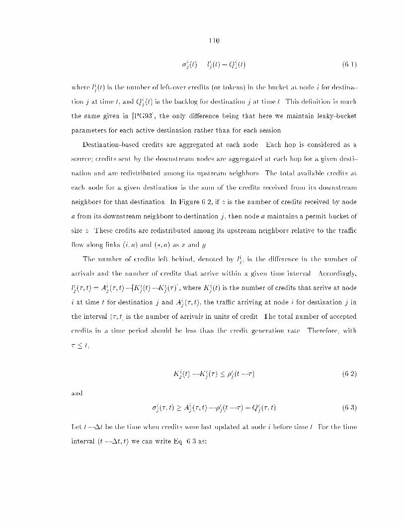
110
�ij(t) = lij(t) + Qij(t) (6.1)
where lij(t) is the number of left-over credits (or tokens) in the bucket at node i for destina-
tion j at time t, and Qij(t) is the backlog for destination j at time t. This de�nition is much
the same given in [PG93], the only di�erence being that here we maintain leaky-bucket
parameters for each active destination rather than for each session.
Destination-based credits are aggregated at each node. Each hop is considered as a
source; credits sent by the downstream nodes are aggregated at each hop for a given desti-
nation and are redistributed among its upstream neighbors. The total available credits at
each node for a given destination is the sum of the credits received from its downstream
neighbors for that destination. In Figure 6.2, if z is the number of credits received by node
a from its downstream neighbors to destination j, then node a maintains a permit bucket of
size z. These credits are redistributed among its upstream neighbors relative to the tra�c
ow along links (i; a) and (s; a) as x and y.
The number of credits left behind, denoted by lij , is the di�erence in the number of
arrivals and the number of credits that arrive within a given time interval. Accordingly,
lij(�; t) = Aij(�; t)� [Ki
j(t)�Kij(�)], where K
ij(t) is the number of credits that arrive at node
i at time t for destination j and Aij(�; t), the tra�c arriving at node i for destination j in
the interval (�; t] is the number of arrivals in units of credit. The total number of accepted
credits in a time period should be less than the credit generation rate. Therefore, with
� � t,
Kij(t)�Ki
j(�) � �ij(t� �) (6.2)
and
�ij(�; t) � Aij(�; t)� �ij(t � �) +Qi
j(�; t) (6.3)
Let t��t be the time when credits were last updated at node i before time t. For the time
interval (t��t; t) we can write Eq. 6.3 as:
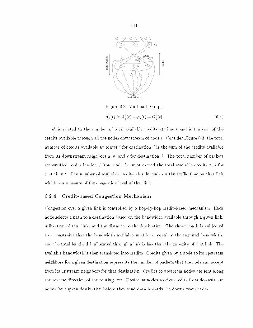
111
j
i WCR
u i
destination j
Dat
a P
acke
ts
ca b
x y z
Cre
ditsSM
d ei
Figure 6.3: Multipath Graph
�ij(t) � Aij(t)� �ij(t) + Qi
j(t) (6.4)
�ij is related to the number of total available credits at time t and is the sum of the
credits available through all the nodes downstream of node i. Consider Figure 6.3, the total
number of credits available at router i for destination j is the sum of the credits available
from its downstream neighbors a, b, and c for destination j. The total number of packets
transmitted to destination j from node i cannot exceed the total available credits at i for
j at time t. The number of available credits also depends on the tra�c ow on that link
which is a measure of the congestion level of that link.
6.2.4 Credit-based Congestion Mechanism
Congestion over a given link is controlled by a hop-by-hop credit-based mechanism. Each
node selects a path to a destination based on the bandwidth available through a given link,
utilization of that link, and the distance to the destination. The chosen path is subjected
to a constraint that the bandwidth available is at least equal to the required bandwidth,
and the total bandwidth allocated through a link is less than the capacity of that link. The
available bandwidth is then translated into credits. Credits given by a node to its upstream
neighbors for a given destination represents the number of packets that the node can accept
from its upstream neighbors for that destination. Credits to upstream nodes are sent along
the reverse direction of the routing tree. Upstream nodes receive credits from downstream
nodes for a given destination before they send data towards the downstream nodes.

112
Figure 6.4 presents a formal description of the credit allocation scheme. Procedure
Initialize indicates the action taken by a node when it becomes active for the �rst time.
Procedure Receive describes the functions performed by a node when a node receives a
periodic update.
Initialization
The number of credits available at each node is determined by the total resources (bu�er
space) available at that node (MaxBufsj). A part of the total available credits (Reserve)
is reserved for a fast reservation mechanism. A fast reservation mechanism is used to
allocate credits to a new source when an explicit credit request is received for a destination.
This mechanism sends a minimum number of credits to the new upstream neighbor as
explained below. This speeds up the credit allocation process, thus avoiding slow start.
Since there is always some reserved credits at each node, nodes upstream do not starve.
The reserved credits which are used for fast reservation when the upstream neighbor/ source
�rst initializes are reclaimed when the tra�c ow through that path starts. The remaining
credits, CRij , are equally distributed among the neighboring nodes, Ni, on startup. This is
termed as the weighted credit WCRijk. The hop-by-hop delay incurred for the credits to
reach next-hop neighbor is incorporated while computing the available credits.
On initialization, credits are equally distributed among neighbors since there will not be
any tra�c on any of the links of a newly established node. Credits are dynamically assigned
thereafter among all the active ows, depending on the tra�c ow through each of the links.
When node i selects neighbor k as one of its multiple successors to a destination, it sets the
successor ag in the update message (flagijk) to that neighbor to indicate that the neighbor
now belongs to shortest multipath set SM ij . When node k recognizes this, it includes the
node in its set of active neighbors, sends a �xed minimum amount of credit (CRmin) to
its new neighbor indicating that i can be a possible multipath successor, and redistributes
its credits for that destination. This information is communicated to other nodes in the
next update interval. The total credits sent to the upstream neighbor is limited by the total
113
available credits at that node. Credit information at each node is updated periodically. This
is required since we are not using any reliable mechanism for updating credit information.
Each routing node resets its tra�c counters and monitors the incoming and outgoing
tra�c for all its neighbors. Based on this statistics, the routing parameters �ijk are com-
puted. The permit bucket parameters are also initialized for each destination. The token
generation rate �ij is initialized to the sum of the credits available through all the neighbors
of i to a given destination j in the given time period. The bucket size �ij is initialized to
the number of leftover packets since on initialization there is no backlog.
Steady State
Each node monitors the tra�c owing through its incoming and outgoing links periodically
and determines the tra�c ow on each of its links for all destinations. A periodic update
timer is maintained at each router to exchange credit information periodically. The periodic
update interval �t should be at least longer than the maximum round trip time (RTT) delay
between two nodes in the network. Each time an update is sent, the timer, timerij , is reset
(Figure 6.4).
At each node, credits received from all downstream nodes are aggregated and are redis-
tributed to the upstream neighbors. This can be done because the total bandwidth allocated
at each link at any given time is no more than the capacity of that link. A node can send
data packets to a downstream neighbor only if the credit value through that neighbor is
greater than zero. Also, because at each hop credits are distributed based on the tra�c
ow, the algorithm ensures that information about all active destinations are maintained,
i.e., those for which data tra�c needs to ow from or through that node. When a new
destination for which the bandwidth is not reserved becomes active, or when a node be-
comes part of the set of loop-free paths to a destination, credits are redistributed using a
fast reservation mechanism.
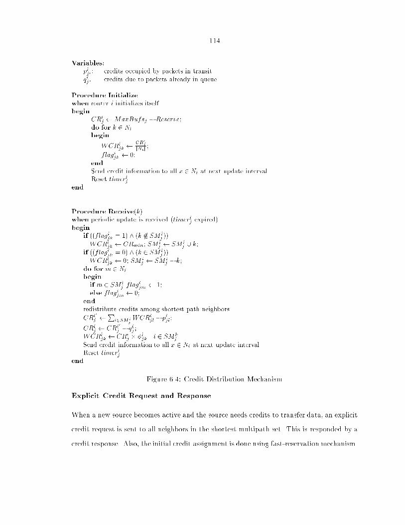
114
Variables:
pijl: credits occupied by packets in transitqij: credits due to packets already in queue
Procedure Initialize
when router i initializes itselfbegin
CRij MaxBufsj � Reserve;
do for k 2 Ni
begin
WCRijk
CRij
jNij;
flagijk 0;end
Send credit information to all x 2 Ni at next update intervalReset timerij
end
Procedure Receive(k)when periodic update is received (timerij expired)begin
if ((flagijk = 1) ^ (k 62 SM ij ))
WCRijk CRmin; SM i
j SM ij [ k;
if ((flagijk = 0) ^ (k 2 SM ij ))
WCRijk 0; SM i
j SM ij � k;
do for m 2 Ni
begin
if m 2 SM ij flag
ijm 1;
else flagijm 0;end
redistribute credits among shortest path neighbors
CRi0
j P
l2SMijWCRi
jl � pijl;
CRij CRi0
j � qij;
WCRijk CRi
j � �ijk j i 2 SMkj
Send credit information to all x 2 Ni at next update intervalReset timerij
end
Figure 6.4: Credit Distribution Mechanism
Explicit Credit Request and Response
When a new source becomes active and the source needs credits to transfer data, an explicit
credit request is sent to all neighbors in the shortest multipath set. This is responded by a
credit response. Also, the initial credit assignment is done using fast-reservation mechanism.

115
Explicit credit response indicates the amount of credits allocated by the destination through
multiple paths for the ow requested.
Explicit Teardown
A teardown message reclaims the credits allocated to a ow. Each teardown message is
associated with a sequence number representing the ow. Although it is not necessary to
explicitly reclaim the credits of a ow, it is recommended that all sources send explicit
teardown message as soon as a session is completed.
Teardown message is initiated by a source and is forwarded hop-by-hop all the way to
the destination. The state of a node is updated along the way and the credits are reclaimed.
These messages are not delivered reliably. The loss of a teardown message will not cause a
protocol failure because the unused credits will eventually time out and are reclaimed.
One-Pass Reservation Mechanism
To ensure that there is no starvation in the protocol, a fast reservation mechanism is used.
This enables the downstream nodes to respond immediately without having to wait till the
nodes hear from their destinations about the credit availability. This scheme is similar to
one-pass reservation mechanism of RSVP [ZDE+93].
Sources send explicit credit requests to a destination requesting credits for data trans-
mission. On receiving these requests, credits are allocated for that session; source and all
the nodes along the way are informed about this. Credits indicate the rate at which a source
can send data to respective destinations.
Each node maintains a soft-state information about the network state. The state infor-
mation is periodically refreshed by periodic credit updates. If a credit update is not received
before certain time interval, those credits are reclaimed. At each periodic timeout interval,
the state of the network is updated. The soft-state information has the potential to change
every periodic time interval.

116
Periodic Updates
Credit (resource reservation) information is updated periodically. The allocated resources
are reclaimed after a certain time if the state information is not refreshed. The timer value
for updating the state information is set at each hop independently. Floyd and Jacobson
[FJ94] have shown that periodic updates generated by independent network nodes can be-
come synchronized. This can lead to disruption in network services as the periodic messages
contend with other network tra�c for link and forwarding resources. Therefore, periodic
credit update messages must avoid synchronization and ensure that any synchronization
that may occur is not stable.
Because of this, the refresh timer should be randomly set to a value in the range [0.5R,
1.5R] where R is the periodic update timer used to generate updates. The value R is chosen
locally at each node. A smaller R speeds up the adaptation to network state changes but
increases the protocol overhead. A node may therefore adjust the e�ective R dynamically
to control the amount of overhead due to periodic update messages. The default value of
R is set to 30 seconds
The end-to-end delay associated with packets to each destination are also estimated
periodically. If the measured delay does not satisfy the required QoS, that successor will
no longer be selected as a feasible successor to that destination and this information is
communicated to all the neighboring nodes. It then determines the total available credits
for a given destination j and the credits are redistributed among its upstream neighbors
after reserving a fraction of the credits for the initialization phase. The philosophy behind
this fast reservation mechanism is similar to a fast bandwidth reservation scheme in which,
the data transmission begins before a connection has been completely established.
Figure 6.5 shows the distance table at node i for destination j for the con�guration in
Figure 6.3. The ag �eld indicates whether the neighbor belongs to the shortest multipath
set or not. The distance gives the sum of the link costs along the path to destination j and
credits gives the number of available credits through that path. A credit of 0 implies that
packets cannot be forwarded through that path.

117
FlagDestination Distance Credits
j
j
j
j
j
j
j
j
a
c
d
e
x
Neighbor
y
z
b
1
1
1
0
0
0
0
0
a1
b1
c1
d1
e1
b2
c2
0
0
0
0
0
a2
x1
y1
z1
Figure 6.5: Distance Table at node i for destination j
The number of credits available at a node is determined by the ow on its links and
the total tra�c seen by that node. If fkji is the incoming ow on link (k; i) to destination
j as seen by node i, and rij is the tra�c originated at i for destination j, we de�ne the
total input tra�c seen by i for destination j as the sum of all the incoming tra�c at node
i, and denote it by tij . Furthermore, by the conservation of ow, the sum of all the tra�c
arriving at a node must be equal to the sum of all the tra�c departing from a node for
each destination j. Therefore, for destination j, the total incoming ow is equal to the total
outgoing ow at node i, and
tij =X
k j i2SMkj
[fkji] + rij =X
m 2 SM ij
f ijm (6.5)
For convenience, a routing variable, denoted by �ijk, is de�ned for each link (i; k) as the
ratio of the ow on each link with respect to the total ow on all outgoing links for a given
destination j. From Eq. 6.5 and with Ni denoting the neighbor set of i, we have:
�ijk =f ijk
tij8k 2 Ni (6.6)
Because node i itself can also contribute to the total tra�c, by the conservation of ow,
it must be true thatX
k2SM ij
�ijk � 1 (6.7)

118
The distribution of credits to upstream neighbors depends on the tra�c ow on that
link, which in turn depends on the routing variable �ij associated with that link. The num-
ber of credits a node sends to an upstream neighbor is called the weighted credit (WCR).
Credits are weighted by the tra�c ow on a given link. The token generation rate for a
given update period �t can now be de�ned as
�ij(t) =Credits available in update period before t
�t
�ij(t) =
PSM ij
k=1 WCRijk(t)
�t(6.8)
To obtain a correct estimate of the credits available at each node at any given time, we
need to take into account the delay associated with the propagation of credits. This can
be done either by estimating the credits available as in [KTA94] or by explicitly sending a
marker. We opt for the estimation mechanism. Credits are sent to the immediate upstream
neighbor, i.e., they propagate only one hop. The update period used for updating routing
information is considered as one round-trip delay by a data packet. Therefore, to obtain a
correct estimate of the available credits at a node, we have to take into account the data
packets that a sender has already forwarded over the link in the previous round-trip time
(RTT) and the data packets that are already queued from the past RTT. Therefore, the total
available credits at node i for a destination j, denoted by CRij, is the di�erence between the
sum of all the weighted credits available from its downstream neighbors di (equivalently,
sum of all the credits on its outgoing links) belonging to the shortest multipath and the
credits which are already being used, i.e.,
CRij =
X
l 2 SM ij
[WCRijl � pijl]� qij (6.9)
where WCRijl is the weighted credit obtained from the downstream neighbor l over an
update period (which depends on the ow on the link (i; l)), pijl is the number of credits

119
occupied by the packets that are already in transit on link (i; l), and qij is the number of
credits due to the data packets that are already in the queue at node i for destination j
which were not completely transmitted since the previous update period. If a node does
not have credits for a given destination j, then CRij is set to zero.
6.2.5 Correctness of Credit-based Scheme
The correctness of the credit based mechanism (i.e., showing that it has no deadlocks
and that packets are not dropped) can be proven in a similar way as for virtual-circuit
connections [OSV94]. For the purposes of such a proof, we make the following assumptions.
� protocol is initialized properly i.e., all nodes have correct credit and routing informa-
tion
� there are no link errors or link and node failures (steady state)
Lemma 6.1 The congestion-oriented credit mechanism never drops packets accepted into
the network.
Proof: The total credits available at a node is given by:
CRij �X
l2SM ij
[WCRijl � pijl]� qij
Also, the total available credits is less than the maximum bu�er space at a node.
MaxBuffersj � CRij
This is true since we reserve some bu�er space (credits) for the fast reservation mecha-
nism.
At any node, the number of credits available for a given destination j is at least equal
to the packets sent downstream for that destination. This is true since a packet can not
be forwarded unless we have a credit to do so. If a packet is in ight from a sender to a
receiver, then pijl = 0 and CRij < MaxBuffersj . Thus, the received packet will not be
dropped as there is at least one empty bu�er that can be used.
120
This proves the Lemma. 2
Lemma 6.2 The credit based mechanism is starvation free.
Proof: To prove this Lemma, we consider three cases { (a) initialization (b) when the
nodes are active and (c) when a explicit credit request is received.
Case (a): On initialization, when a new node comes up, the node distributes its credits
equally among its neighbors and receives a minimum number of non-zero credits from its
neighbors indicating the presence of a possible path to a destination through that neighbor.
Therefore, on startup since always a minimum number of credits are available to the new
node, the credit mechanism is starvation free.
Case (b): When a new node becomes a member of the shortest multipath set (SM ij), the
successor ag will be set in the update message. On receiving this update, the neighbor
sends a minimum number of credits initially using the reserved bandwidth available through
the fast reservation mechanism and later on dynamically updates the credits depending on
the tra�c on the link.
Case (c): An explicit request for credits from a source is received by means of a routing
table update. This update sets the successor ag in the update message. Therefore, the
message will be treated as any other routing table update and is processed similar to case
(b) if the router has credits to send to its upstream neighbors. Otherwise, the router
sends routing table updates to its shortest multipath neighbors (downstream neighbors)
requesting for credits to send packets to the destination. In the worst-case, this process
can continue till the routing table update reaches the destination and will terminate at the
destination.
This ensures that a node will always have credits when it requires to forward a packet.
Therefore, the protocol is starvation free. 2
Theorem 7 In the congestion-based credit mechanism, if there is a packet at a node to be
sent, it will be eventually sent.

121
Proof: From Lemma 6.1, packets are not dropped. Therefore, packet arriving at a node
will either be queued or is forwarded. From Lemma 6.2, whenever a node needs to forward
a packet, it always has the credits to do so.
Therefore, packets arriving at a node will be always sent eventually. Of course, when
links or nodes fail, packets accepted in the network may have to be dropped. The same
occurs in a connection-oriented architecture when resources fail along a connection already
established. This proves the theorem 2
6.2.6 Maintenance of Loop-Free Multipaths
The primary objective of maintaining multiple loop-free paths is to minimize the end-to-
end path delay by reducing network congestion along the path. The distance reported by
neighbor k to node i for destination j is denoted by Dijk and node i's distance to its neighbor
k is denoted by dik. The distance to neighbor k is the sum of the propagation delay �ik and
the per hop packet delay through neighbor k, dijk. i.e., dik = dijk + �ik . The path delay at
node i along node k at a given time t, denoted by �Dijk is
�Dijk = Di
jk + dik.
The shortest multipath set of i for destination j (SM ij) is a set of neighbors of i that
provide loop-free paths to j. The delay at node i to destination j at time t is computed as
the weighted average path delay through all the nodes in the shortest multipath at node i;
it is denoted by Dij(t). This delay is weighted by the fraction of the tra�c going through
that path, i.e.,
Dij(t) =
X
k2SMij(t)
�ijk(t): �Dijk(t) =
X
k2SMij(t)
f ijk(t)
tij(t): �Di
jk(t) (6.10)
The ow from i to each neighbor in SM ij depends on the credits available through that
neighbor. Assuming that packets are of �xed size and that each packet corresponds to one
credit, we can say that a packet ows on a link if at least one credit is available on that
link. This implies that the number of packets that can ow on a link is equal to the number
of credits available through that link; therefore,
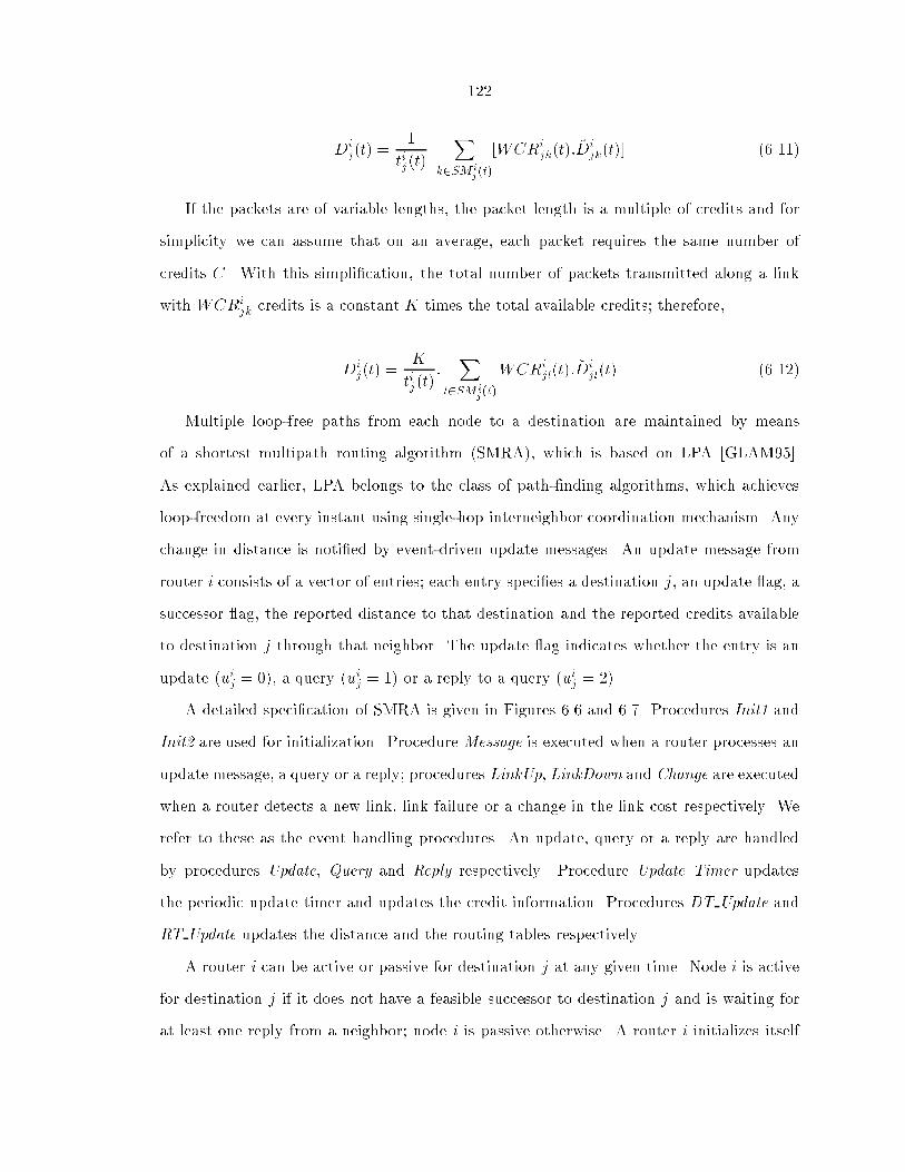
122
Dij(t) =
1
tij(t)
X
k2SM ij(t)
[WCRijk(t): �D
ijk(t)] (6.11)
If the packets are of variable lengths, the packet length is a multiple of credits and for
simplicity we can assume that on an average, each packet requires the same number of
credits C. With this simpli�cation, the total number of packets transmitted along a link
with WCRijk credits is a constant K times the total available credits; therefore,
Dij(t) =
K
tij(t):X
l2SM ij(t)
WCRijl(t):
�Dijl(t) (6.12)
Multiple loop-free paths from each node to a destination are maintained by means
of a shortest multipath routing algorithm (SMRA), which is based on LPA [GLAM95].
As explained earlier, LPA belongs to the class of path-�nding algorithms, which achieves
loop-freedom at every instant using single-hop interneighbor coordination mechanism. Any
change in distance is noti�ed by event-driven update messages. An update message from
router i consists of a vector of entries; each entry speci�es a destination j, an update ag, a
successor ag, the reported distance to that destination and the reported credits available
to destination j through that neighbor. The update ag indicates whether the entry is an
update (uij = 0), a query (uij = 1) or a reply to a query (uij = 2).
A detailed speci�cation of SMRA is given in Figures 6.6 and 6.7. Procedures Init1 and
Init2 are used for initialization. Procedure Message is executed when a router processes an
update message, a query or a reply; procedures LinkUp, LinkDown and Change are executed
when a router detects a new link, link failure or a change in the link cost respectively. We
refer to these as the event handling procedures. An update, query or a reply are handled
by procedures Update, Query and Reply respectively. Procedure Update Timer updates
the periodic update timer and updates the credit information. Procedures DT Update and
RT Update updates the distance and the routing tables respectively.
A router i can be active or passive for destination j at any given time. Node i is active
for destination j if it does not have a feasible successor to destination j and is waiting for
at least one reply from a neighbor; node i is passive otherwise. A router i initializes itself
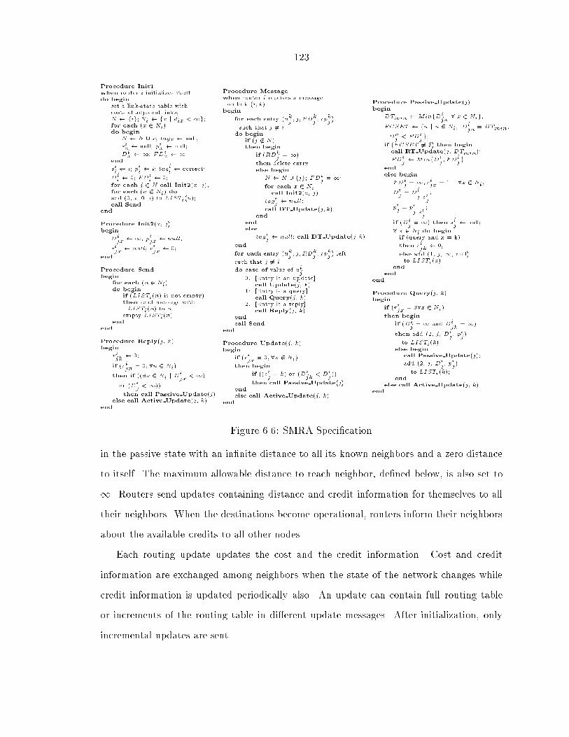
123
Procedure Init1when router i initializes itselfdo begin
set a link-state table withcosts of adjacent links;N fig;Ni fx j dix <1g;for each (x 2 Ni)do begin
N N [ x; tagx null;
six null; pix null;
Dix 1; FDix 1end
sii i; pi
i i; tagi
i correct;
Dii 0; FDi
i 0;
for each j 2 N call Init2(x, j);for each (n 2 Ni) doadd (0, i, 0, i) to LISTi(n);call Send
end
Procedure Init2(x, j)begin
Dijx 1; pi
jx null;
sijx null; ri
jx 0;
end
Procedure Sendbegin
for each (n 2 Ni)do begin
if (LISTi(n) is not empty)then send message withLISTi(n) to n
empty LISTi(n)end
end
Procedure Reply(j, k)begin
rijk 0;
if (rijn
= 0; 8n 2 Ni)
then if ((9x 2 Ni j Dijx
<1)
or (Dij<1))
then call Passive Update(j)else call Active Update(j, k)
end
Procedure Messagewhen router i receives a messageon link (i; k)
begin
for each entry (ukj; j;RDk
j; rpk
j)
such that j 6= i
do beginif (j 62 N)then begin
if (RDkj= 1)
then delete entryelse begin
N N [ fjg; FDij=1;
for each x 2 Nicall Init2(x, j)
tagij null;
call DT Update(j; k)end
endelse
tagij null; call DT Update(j; k)
end
for each entry (ukj; j;RDk
j; rpk
j) left
such that j 6= i
do case of value of uij
0: [Entry is an update]call Update(j, k)
1: [Entry is a query]call Query(j, k)
2: [Entry is a reply]call Reply(j, k)
endcall Send
end
Procedure Update(j, k)begin
if (rijx
= 0; 8x 2 Ni)
then begin
if ((sij= k) or (Di
jk< Di
j))
then call Passive Update(j)endelse call Active Update(j, k)
end
Procedure Passive Update(j)begin
DTmin MinfDijx8 x 2 Nig;
FCSET fn j n 2 Ni; Dijn
= DTmin,
Dnj< FDi
jg;
if (FCSET 6= ;) then begincall RT Update(j, DTmin);
FDij MinfDi
j; FDi
jg
endelse begin
FDij= 1; ri
jx= 1; 8x 2 Ni ;
Dij= Di
j sij
;
pij= pi
j sij
;
if (Dij=1) then si
j null;
8 x 2 Ni do beginif (query and x = k)
then rijk 0;
else add (1, j, 1, null)to LISTi(x)
endend
end
Procedure Query(j, k)begin
if (rijx
= 08x 2 Ni)
then begin
if (Dij= 1 and Di
jk=1)
then add (2, j, Dij, pi
j)
to LISTi(k)else begin
call Passive Update(j);
add (2, j, Dij, pij)
to LISTi(k);end
else call Active Update(j, k)end
Figure 6.6: SMRA Speci�cation
in the passive state with an in�nite distance to all its known neighbors and a zero distance
to itself. The maximum allowable distance to reach neighbor, de�ned below, is also set to
1. Routers send updates containing distance and credit information for themselves to all
their neighbors. When the destinations become operational, routers inform their neighbors
about the available credits to all other nodes.
Each routing update updates the cost and the credit information. Cost and credit
information are exchanged among neighbors when the state of the network changes while
credit information is updated periodically also. An update can contain full routing table
or increments of the routing table in di�erent update messages. After initialization, only
incremental updates are sent.
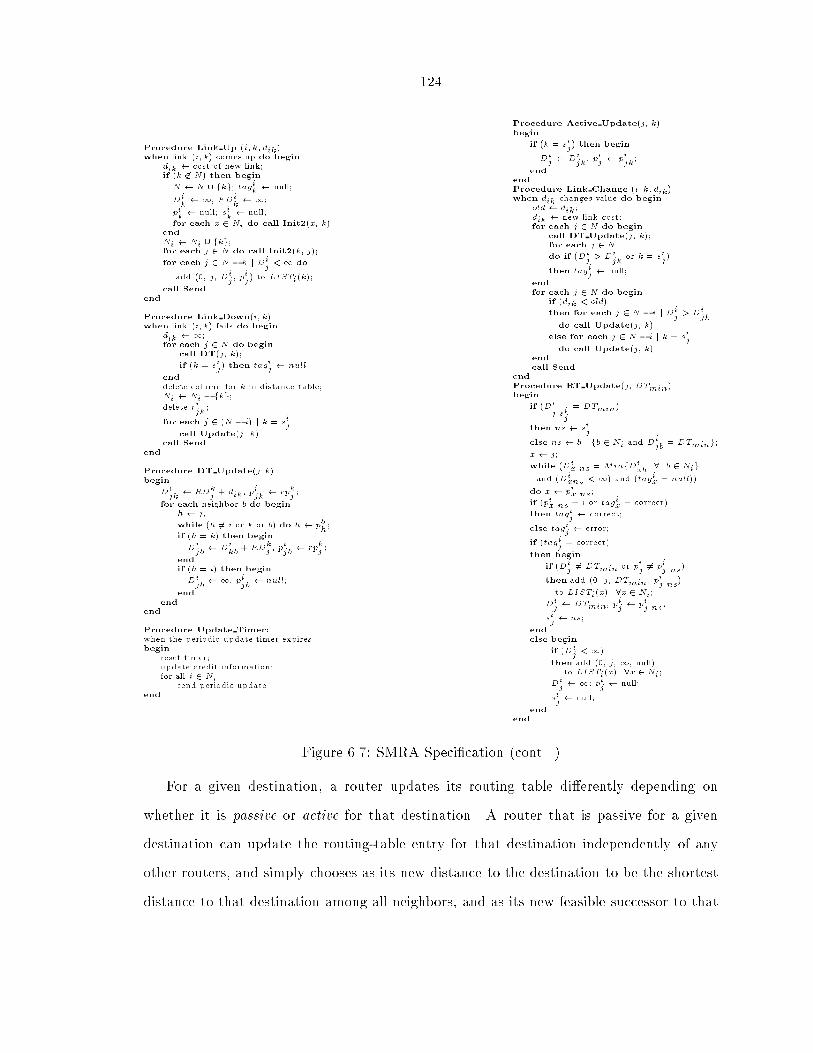
124
Procedure Link Up (i; k; dik)when link (i; k) comes up do begin
dik cost of new link;if (k 62 N) then begin
N N [ fkg; tagik null;
Dik 1; FDi
k 1;
pik null; si
k null;
for each x 2 Ni do call Init2(x, k)endNi Ni [ fkg;for each j 2 N do call Init2(k, j);
for each j 2 N � k j Dij<1 do
add (0, j, Dij, pij) to LISTi(k);
call Sendend
Procedure Link Down(i; k)when link (i; k) fails do begin
dik 1;for each j 2 N do begin
call DT(j, k);
if (k = sij) then tagi
j null
end
delete column for k in distance table;Ni Ni � fkg;
delete rijk
;
for each j 2 (N � i) j k = sij
call Update(j, k)call Send
end
Procedure DT Update(j; k)begin
Dijk RDk
j+ dik ; p
ijk rpk
j;
for each neighbor b do beginh j;
while (h 6= i or k or b) do h pbh;
if (h = k) then begin
Dijb Di
kb+ RDk
j; pijb rpk
j;
endif (h = i) then begin
Dijb 1; pi
jb null;
endend
end
Procedure Update Timer:when the periodic update timer expiresbegin
reset timer;update credit information;for all i 2 Ni
send periodic update;end
Procedure Active Update(j, k)begin
if (k = sij) then begin
Dij Di
jk; pij pi
jk;
endendProcedure Link Change (i; k; dik)when dik changes value do begin
old dik ;dik new link cost;for each j 2 N do begin
call DT Update(j, k);for each j 2 N
do if (Dij> Di
jkor k = si
j)
then tagij null;
endfor each j 2 N do begin
if (dik < old)
then for each j 2 N � i j Dij> Di
jkdo call Update(j, k)
else for each j 2 N � i j k = sij
do call Update(j, k)endcall Send
endProcedure RT Update(j, DTmin)begin
if (Dij si
j
= DTmin)
then ns sij;
else ns b j fb 2 Ni and Dijb
= DTming;
x j;
while (Dix ns = MinfDixb8 b 2 Nig
and (Dixns <1) and (tagix = null))
do x pix ns;
if (pix ns = i or tagix = correct)
then tagij correct;
else tagij error;
if (tagij= correct)
then begin
if (Dij6= DTmin or pi
j6= pi
j ns)
then add (0, j, DTmin , pij ns
)
to LISTi(x) 8x 2 Ni;
Dij DTmin; p
ij pi
j ns;
sij ns;
endelse begin
if (Dij<1)
then add (0, j, 1, null)to LISTi(x) 8x 2 Ni ;
Dij 1; pi
j null;
sij null;
endend
Figure 6.7: SMRA Speci�cation (cont...)
For a given destination, a router updates its routing table di�erently depending on
whether it is passive or active for that destination. A router that is passive for a given
destination can update the routing-table entry for that destination independently of any
other routers, and simply chooses as its new distance to the destination to be the shortest
distance to that destination among all neighbors, and as its new feasible successor to that

125
destination to be any neighbor through whom the shortest distance is achieved. In contrast,
a router that is or becomes active for a given destination must synchronize the updating of
its routing-table entry with other routers.
When a router is passive and needs to update its routing table for a given destination
j after it processes an update message from a neighbor or detects a change in the cost
or availability of a link or a change in the credit information, it tries to obtain a feasible
successor. From router i's standpoint, a feasible successor toward destination j is a neighbor
router k that satis�es the maximum allowable distance condition (MADC) given by the
following two equations [GLAM95]:
Dij = Di
jk + dik =MinfDijp + dip j p 2 Nig
Dijk < MADi
j (6.13)
where MADij is the maximum allowable distance for destination j, and is equal to the
minimum value obtained for Dij since the last time router i transitioned from active to
passive state for destination j. Router i adjusts MADij depending on the congestion level
of the network.
If router i �nds a feasible successor, it remains passive and updates its routing-table entry
as in the Distributed Bellman-Ford algorithm [BG92]. Alternatively, if router i cannot �nd
a feasible successor, it �rst sets its distance equal to the addition of the distance reported
by its current successor and the cost of the link to that neighbor. The router also sets
its maximum allowable distance equal to its new distance. After updating its tables, a
router becomes active by sending a query in an update message to all its neighbors; such
a query speci�es the router's new distance through its current successor. It then sets the
destination's reply-status table entry for each link to one, indicating that it expects a reply
from each neighbor for that destination.
Once active for destination j, router i cannot change its feasible successor, MADij , the
value of the distance it reports to its neighbors, or its entry in the routing table, until it
126
receives all the replies to its query. A reply received from a neighbor indicates that such
a neighbor has processed the query and has either obtained a feasible successor to the
destination, or determined that it cannot reach the destination. After node i obtains all
the replies to its query, it computes a new distance and successor to destination j, updates
its feasible distance to equal its new distance, and sends an update to all its neighbors.
Multiple changes in link cost or availability are handled by ensuring that a given node is
waiting to complete the processing of at most one query at any given time. The mechanism
used to accomplish this is speci�ed in [GLAM95], and is such that a node can be either
passive or in active state, and it processes any pending update or distance increases that
occurred while it was active.
Ensuring that updates will not be sent in the network when some destination is unreach-
able is easily done. If node i has set Dij =1 already and receives an input event (a change
in cost or status of link (i; k), or an update or query from node k) such that Dijk+dik =1,
then node i simply updates Dijk or dik, and sends a reply to node k with RDi
j = 1 if
the input event is a query from node k. When an active node i has an in�nite maximum
allowable distance and receives all the replies to its query such that every neighbor o�ers
an in�nite distance to the destination, the node simply becomes passive with an in�nite
distance.
When node i establishes a link with a neighbor k, it updates the value of dik and assumes
that node k has reported in�nite distances to all destinations and has replied to any query
for which node i is active. Furthermore, if node k is a previously unknown destination, node
i sets sik = null, and Dik = RDi
k = MADik = 1. Node i also sends to its new neighbor k
an update for each destination for which it has a �nite distance.
When node i is passive and detects that link (i; k) has failed, it sets dik = 1 and
�Dijk =1. After that, node i carries out the same steps used for the reception of a link-cost
change in the passive state.
Because a router can become active in only one interneighbor coordination mechanism
per destination at a time, it can expect at most one reply from each neighbor. Accordingly,

127
dist
ance
Q Q
MAD
All Replies inFirst Successor
MADij = Min { D
i }
Initialization to infinity
Distance
j
SynchronizationPoint time
Figure 6.8: Maximum Allowable Distance Condition
when an active node i loses connectivity with a neighbor n, node i can set rijn = 0 and
Dijn =1, i.e., assume that its neighbor n has sent any required reply reporting an in�nite
distance. When node i becomes passive again, it must �nd a neighbor that satis�es the
MADC using the value of MADij set at the time node i became active in the �rst place.
After �nding a new successor, the permit bucket parameters �ij and �ij are also updated.
Figure 6.8 gives a graphical representation of how MAD is updated. The point at which
a new di�using computation starts is a synchronization point. It can be noted that between
two synchronization points the value of MAD can only decrease or remain the same. This
ensures that the algorithm is loop-free.
To route packets to a destination j, each router uses the following rule to select the
neighbor routers that should belong to its shortest multipaths for j:
Shortest Multipath Condition (SMC): At time t, router i can make node k 2 Ni(t) part of
SM ij if and only if Di
jk(t) < MADij(t).
When nodes choose their successors using SMC, the path from source to destination
obtained as a result of this is loop free at every instant. The proof of correctness and
loop-freedom of SMRA is basically the same as that provided in [GLAM95] for LPA.
6.3 Worst-Case Steady-State Delay
In this section, we derive an upper bound on the end-to-end steady-state path delay from
node i to destination j (Di�j ) as a function of the credits available through each path under
steady state. Steady-state means that all distances and credit information is correct at every
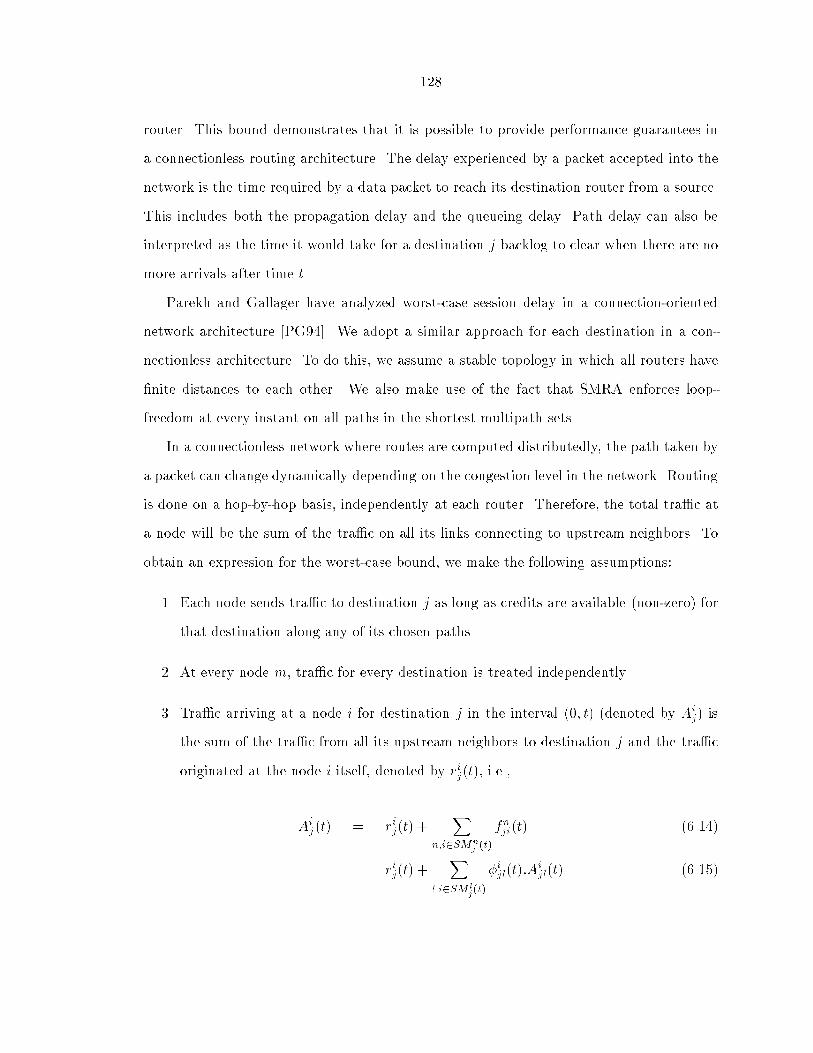
128
router. This bound demonstrates that it is possible to provide performance guarantees in
a connectionless routing architecture. The delay experienced by a packet accepted into the
network is the time required by a data packet to reach its destination router from a source.
This includes both the propagation delay and the queueing delay. Path delay can also be
interpreted as the time it would take for a destination j backlog to clear when there are no
more arrivals after time t.
Parekh and Gallager have analyzed worst-case session delay in a connection-oriented
network architecture [PG94]. We adopt a similar approach for each destination in a con-
nectionless architecture. To do this, we assume a stable topology in which all routers have
�nite distances to each other. We also make use of the fact that SMRA enforces loop-
freedom at every instant on all paths in the shortest multipath sets.
In a connectionless network where routes are computed distributedly, the path taken by
a packet can change dynamically depending on the congestion level in the network. Routing
is done on a hop-by-hop basis, independently at each router. Therefore, the total tra�c at
a node will be the sum of the tra�c on all its links connecting to upstream neighbors. To
obtain an expression for the worst-case bound, we make the following assumptions:
1. Each node sends tra�c to destination j as long as credits are available (non-zero) for
that destination along any of its chosen paths.
2. At every node m, tra�c for every destination is treated independently.
3. Tra�c arriving at a node i for destination j in the interval (0; t) (denoted by Aij) is
the sum of the tra�c from all its upstream neighbors to destination j and the tra�c
originated at the node i itself, denoted by rij(t), i.e.,
Aij(t) = rij(t) +
X
n;i2SMnj (t)
fnji(t) (6.14)
= rij(t) +X
lji2SM lj(t)
�ijl(t):Aijl(t) (6.15)
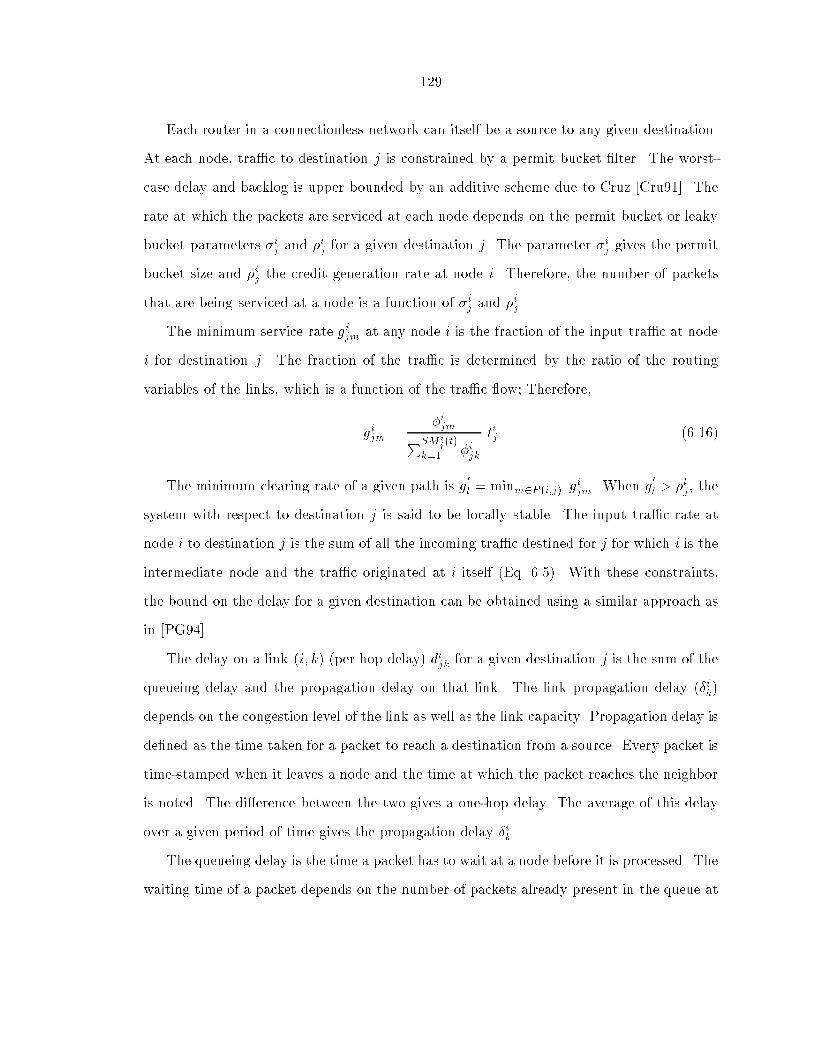
129
Each router in a connectionless network can itself be a source to any given destination.
At each node, tra�c to destination j is constrained by a permit bucket �lter. The worst-
case delay and backlog is upper bounded by an additive scheme due to Cruz [Cru91]. The
rate at which the packets are serviced at each node depends on the permit bucket or leaky
bucket parameters �ij and �ij for a given destination j. The parameter �ij gives the permit
bucket size and �ij the credit generation rate at node i. Therefore, the number of packets
that are being serviced at a node is a function of �ij and �ij.
The minimum service rate gijm at any node i is the fraction of the input tra�c at node
i for destination j. The fraction of the tra�c is determined by the ratio of the routing
variables of the links, which is a function of the tra�c ow; Therefore,
gijm =�ijm
PSM ij(t)
k=1 �ijk
tij (6.16)
The minimum clearing rate of a given path is g0
l = minm2P (i;j) gijm. When g
0
l > �lj , the
system with respect to destination j is said to be locally stable. The input tra�c rate at
node i to destination j is the sum of all the incoming tra�c destined for j for which i is the
intermediate node and the tra�c originated at i itself (Eq. 6.5). With these constraints,
the bound on the delay for a given destination can be obtained using a similar approach as
in [PG94].
The delay on a link (i; k) (per hop delay) dijk for a given destination j is the sum of the
queueing delay and the propagation delay on that link. The link propagation delay (�ik)
depends on the congestion level of the link as well as the link capacity. Propagation delay is
de�ned as the time taken for a packet to reach a destination from a source. Every packet is
time-stamped when it leaves a node and the time at which the packet reaches the neighbor
is noted. The di�erence between the two gives a one-hop delay. The average of this delay
over a given period of time gives the propagation delay �ik.
The queueing delay is the time a packet has to wait at a node before it is processed. The
waiting time of a packet depends on the number of packets already present in the queue at
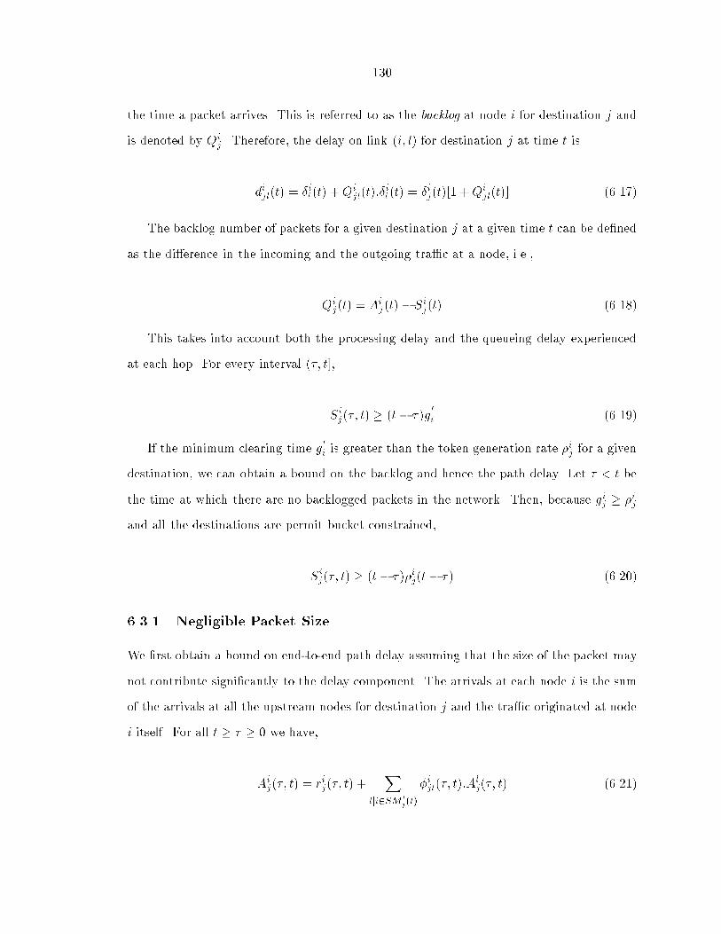
130
the time a packet arrives. This is referred to as the backlog at node i for destination j and
is denoted by Qij . Therefore, the delay on link (i; l) for destination j at time t is
dijl(t) = �il(t) +Qijl(t):�
il(t) = �ij(t)[1 +Qi
jl(t)] (6.17)
The backlog number of packets for a given destination j at a given time t can be de�ned
as the di�erence in the incoming and the outgoing tra�c at a node, i.e.,
Qij(t) = Ai
j(t)� Sij(t) (6.18)
This takes into account both the processing delay and the queueing delay experienced
at each hop. For every interval (�; t],
Sij(�; t) � (t� �)g
0
i (6.19)
If the minimum clearing time g0
i is greater than the token generation rate �ij for a given
destination, we can obtain a bound on the backlog and hence the path delay. Let � < t be
the time at which there are no backlogged packets in the network. Then, because gij � �ij
and all the destinations are permit bucket constrained,
Sij(�; t) � (t � �)�ij(t � �) (6.20)
6.3.1 Negligible Packet Size
We �rst obtain a bound on end-to-end path delay assuming that the size of the packet may
not contribute signi�cantly to the delay component. The arrivals at each node i is the sum
of the arrivals at all the upstream nodes for destination j and the tra�c originated at node
i itself. For all t � � � 0 we have,
Aij(�; t) = rij(�; t) +
X
lji2SM lj(t)
�ijl(�; t):Alj(�; t) (6.21)

131
The maximum backlog tra�c Qi�j for destination j is the di�erence between the arrivals
in the interval (�; t] and the total packets serviced in the same interval at node i. For
�ijl > 0,
Qi�j (�; t) � Ai
j(�; t)� Sij(�; t) (6.22)
Qi�j (�; t) � rij(�; t)� Si
j(�; t)
+X
lji2SM lj(t)
[�ijl(�; t):Alj(�; t)] (6.23)
Qi�j (�; t) � [rij(t)� rij(�)]� Si
j(�; t)
+X
lji2SM lj(t)
[�ijl(�; t):Alj(�; t)] (6.24)
The di�erence (rij(t)� rij(�)) determines the amount of tra�c arriving at node i in the
interval (t � �); the maximum of which is the sum of the tokens available at node i and
the tokens received in the interval (t � �). At every node, each destination is constrained
independently by a permit bucket scheme. Following Parekh and Gallager's approxima-
tion [PG94], we assume the links to be of in�nite capacity. The results for the in�nite
capacity case upper-bound the �nite capacity case. In other words, the results of in�nite
capacity can be used for any �nite speed link. The arrival and the service functions at each
router can be translated to permit bucket parameters, which in turn depend on the maxi-
mum tolerable path delay and the link ows. Substituting for the arrivals and the number
of packets serviced in terms of the permit bucket parameters from the previous section we
have
Qi�j (�; t) � [�ij(t � �) + �ij(t� �)]� �ij(t� �)
+X
lji2SM lj(t)
f ijl
tij[�ij(t� �) + �ij(t� �)]
Becausef ijl
tij
� 1 for any j and l 2 SM ij(t),

132
Qi�j (�; t) � �ij(t� �) +
X
l j i2SM lj(t)
[�lj(t� �) + �lj(t � �)] (6.25)
Making � = t��t, we can write
Qi�j (t) � �ij(t) +
X
l j i2SM lj(t)
[�lj(t) + �lj(t)]
Therefore, the backlog at node i to destination j depends on the leaky bucket parameters
at node i and the permit bucket parameters of all the upstream neighbors of i for which
node i is in the shortest multipath set.
The delay at each node i can be computed as the weighted average path delay through
all its multipath neighbors; therefore,
Dij(t) =
X
k2SM ij(t)
�ijk(t) �Dijk(t) (6.26)
The distance from i to j through neighbor k can be expressed as the sum of the distance
from k to j and the link cost from i to k. The link cost is the sum of the distance and the
propagation delay of that link. Therefore,
�Dijk(t) = Di
jk(t) + dik(t) = Dijk(t) + [dijk(t) + �ik(t)]
Dij(t) =
X
k2SM ij(t)
�ijk(t)[Dijk(t) + (dik(t) + �ik)(t)] (6.27)
From Eq. 6.17, dik(t) = �ik(t)[1 +Qij(t)], which implies that
Dij(t) =
X
k2SM ij(t)
�ijk(t)[Dijk(t) + �ik(t)(1 + Qi
j(t))] (6.28)
Because SMC must be satis�ed by every k 2 SM ij(t), D
ijk(t) < MADi
j(t). Then, if
Dij(�) is the maximum path delay from i to j at time � and Qi�
j (t) is the maximum backlog
from i to j at time t, we obtain from Eq. 6.28 that
Di�j (t) <
X
k2SM ij(t)
[�ijk(t):�ik(t)(1 +Qi�
j )(t)]

133
+MADij(t)
X
k2SM ij(t)
�ijk(t) (6.29)
Let the maximum link propagation delay of all the links from i to a node in SM ij(t) be
�ij(t) = max
k2SM ij(t)
�ik(t) (6.30)
Therefore, the maximum path delay from i to j becomes
Di�j (t) < �i
j(t)X
k2SM ij(t)
�ijk(t)[1 + Qi�j (t)]
+MADij(t)
X
k2SM ij(t)
�ijk(t) (6.31)
Noticing that Qi�j (t) is independent of k and substituting Eq. 6.7 in Eq. 6.31 we obtain
Di�j (t) < �i
j(t)[1 + Qi�j (t)] +MADi
j(t) (6.32)
The above equation is an upper bound on Dij(t) that should be expected. It states that
Dij(t) must be smaller than the sum of the product of the backlog for i at node i times the
maximum link propagation delay in node i's shortest multipath, plus MADij(t). The �rst
term of Eq. 6.32 corresponds to the delay incurred by sending all backlogged packets at
time t to a neighbor with the longest link propagation delay. The second term corresponds
to the maximum delay incurred by any neighbor receiving the backlog packets; because any
such neighbor must be on SM ij(t), that delay can be at most equal to MADi
j(t).
Substituting Eq. 6.25 in Eq. 6.32, we can represent the same bound in terms of permit
bucket parameters as follows:
Di�j (t) < �i
j(t)f1 + �ij(t)X
lji2SMlj(t)
[�lj(t) + �lj(t � � )]g
+MADij(t) (6.33)

134
The bound given by Equations. 6.32 and 6.33 for router i is based on a maximum delay
o�ered by the neighbor of i and a maximum backlog allowed at router i. This is possible
because of two main features of SMRA: datagrams are accepted only if routers have enough
credits to ensure their delivery, and datagrams are delivered along loop-free paths. In
contrast, in traditional datagram routing architectures, any datagram presented to a router
is sent towards the destination, and the paths taken by such datagrams can have loops;
therefore, it is not possible to ensure a �nite delay for the entry router or any relay router
servicing a datagram.
6.3.2 Non-negligible Packet Size
In PGPS networks, routing nodes do not transmit packets until a packet has completely
arrived. Therefore, the number of packets which will reach a downstream node is at the
most equal to the number of packets serviced by its upstream neighbors. Let Li be the
maximum packet size at node i. The PGPS server does not begin servicing a packet until
the last bit has arrived.
For a packet-switched network
Aij(�; t) = rij(�; t) +
X
m j i2SMmj (t)
Smji (�; t) (6.34)
Here, Smji (�; t) represents the number of packets serviced by an upstream neighbor m
for which i is in the shortest multipath to j in the interval (t� �). Let K be the number of
hops in a given path from i to j; m and m� 1 be two successive nodes. Then, for a given
path,
X
m�1
Sm�1jm (�; t) � Am
j (�; t)� rmj (�; t)
�X
m�1
[Sm�1jm (�; t)� Lm�1 (6.35)
where, m = 2; ::::; K; � < t and Lm�1 is the maximum length of a packet transmitted by
node m� 1. Here, the nodes m and (m� 1) are such that m 2 SMm�1j .

135
For a PGPS system, the number of packets serviced for t > � is given as
Sij(�; t) � min
V2[�;t]f[Ai
j(�; V )� rij(�; V )]
+GKj (t� V )g+K:Li (6.36)
where V represents the last time in the interval [�; t] at which node i begins a busy period
for destination j and the function GKj is a convex function which indicates the amount of
service given to destination j under a greedy regime.
Sij(0; t) � minV2[0;t]
f[Aij(0;V)� rij(0;V)]+ GK
j (t� V)g+ K:Li (6.37)
With a greedy regime, the service to destination j is minimized and is delayed by an
appropriate amount, which is given by the minimizing value of V , denoted by Vmin.
Sij(t) � f[Aij(Vmin)� rij(Vmin)] + GK
j (t�Vmin)g+ K:Li (6.38)
The backlog tra�c for a destination j from i is the di�erence between the number of
packets that has arrived and the number of packets serviced as in the previous case.
Qij(0; t) = Ai
j(0; t)� Sij(0; t) (6.39)
Applying similar argument as in the previous section, we have
Qij(t) = �ij(t) + �ij(t) +
X
ljSM ij(t)2l
[�lj(t) + �lj(t)]� Sij(t) (6.40)
Substituting for Sij(t) we have,
Qij(t) = �ij(t) � �
ij(Vmin) �G
mj (t� Vmin) +m:Li
+X
ljSMij(t)2l
[�lj(t) + �lj(t)] (6.41)
Thus, the maximum backlog is given by

136
Qi�j (t) = �ij(t)� �ij(Vmin) +m:Lmax �G
mj (t � Vmin)
+X
ljSMij(t)2l
[�lj(t) + �lj(t)] (6.42)
Having bound the worst-case backlog, we can use a similar approach as in Eq. 6.31 to
obtain bounds for the maximum path delay. Since we are considering a PGPS system, the
expression for maximum path delay becomes
Di�j (t) �MADi
j(t) + �ij(t)
X
lji2SM lj(t)
[1 + Qi�j (t)] (6.43)
Substituting for the maximum backlog from Eq. 6.42 we obtain,
Di�j (t) � MADi
j(t) + �ij(t)
X
lji2SMlj(t)
f1 + �ij(t)� �ij(Vmin)
+m:Lmax � Gmj (t� Vmin)
+X
[�lj(t) + �lj(t)]g (6.44)
Di�j � MADi
j(t) + �ij(t)f1 + �ij(t) � �
ij(Vmin)
+m:Lmax � Gmj (t� Vmin)
+X
lji2SMlj(t)
[�lj(t) + �lj(t)]g (6.45)
Here again, the excess delay experienced by a packet depends on the network tra�c as
earlier. In addition, it also is a function of the packet size and depends on the entire path
from source to a given destination node.
6.4 Two-Tier Architecture
To support end-to-end connections and thereby to guarantee QoS on top of a connectionless
architecture, we model the network as a two-tier architecture. To the end user, the network

137
DOLB
R1
R2
R3
Rn
Weighted Round Robin
COLB
Figure 6.9: Source Model
looks like a connection oriented network through which the user can request for several
levels of QoS as in any connection-oriented scheme. Within the network packets are routed
on a hop-by-hop basis. Routing decisions are made independently at each hop.
6.4.1 End-to-End Model
Each source supports connection-oriented sessions. These sessions exist on top of a con-
nectionless (destination oriented) ow. To the end user, these ows appear as connection-
oriented sessions through which they can reserve resources and can have all the exibility of
a connection oriented architecture. These session based ows are mapped on to destination-
based ows. Each router has the capability to di�erentiate one ow from another.
Figure 6.9 shows the model at a source. Connection-oriented sessions are regulated
by leaky-bucket �lters, which we refer to as connection-oriented leaky buckets (COLB). A
connection oriented session generates tra�c at a rate ri, where i = 1,...N is the number of
sessions that can exist at any time. Each session is identi�ed by a source-destination pair
and the type of service requested by that ow.
6.4.2 Connectionless Model
Connection-oriented sessions for the same destination belonging to the same tra�c class
(QoS type) are grouped together and are mapped into a connectionless ow. The con-
nectionless ows are serviced on a per-destination basis instead of per-session basis as in
connection-oriented architecture. For each set of COLB sessions, a destination-oriented

138
leaky bucket (DOLB) is maintained. This depends on the tra�c class and the destination
of COLB sessions. The way in which COLB ows are fed to DOLB depends on the relative
rates of the associated COLB ows.
To ensure fairness among di�erent connections, a weighted round robin scheduling mech-
anism among all COLB ows belonging to the same group is used at each of DOLB inputs.
Our protocol guarantees that all packets which enter the connectionless network source will
be delivered to their respective destinations, unless a resource failure prevents it. Depending
on the available resources (credits) at each hop, the tra�c entering the network is regulated
at the COLB stage itself, before the packets actually enter the network. This ensures no
packets are dropped once they enter the network. In order to regulate the tra�c ow from
COLBs to DOLB, a feedback mechanism is required from DOLB to COLB, so that the
leaky bucket parameters of COLB can be regulated.
Let there be N connection-oriented sessions associated with each DOLB with tra�c
generation rates of r1, r2,..., rN respectively. Each of these sessions is controlled by leaky-
bucket parameters (�i; �i), where � is the bu�er size and � is the tra�c generation rate.
(�S ; �S) are the leaky-bucket parameters for the corresponding DOLB.
Let CRSj be the total available credits (or tokens) at source S for destination j. The
token generation at each of the COLBs is a function of the available credits. When there
are N active sources the token generation at each DOLB is given by
�i =riPNk=1 rk
CRSj (6.46)
This mechanism ensures that sources are well behaved and DOLB does not accept more
data than it can handle and thus can ensure guaranteed delivery of packets once the packets
enter the network.
6.4.3 Node Model
Figure 6.10 shows the model of a path. Since routing decisions are made at each hop, all
nodes along the path from a source to a destination can be a potential source, contributing

139
jbA
ij
Aa A
j
b
i ja
Permit BucketsPermit Buckets
Figure 6.10: Node Model
to the tra�c ow towards the destination. Therefore, the tra�c at a node corresponds to
the tra�c arriving at a node from its upstream neighbors and the tra�c originated at the
node itself. Scheduling at a node is done by maintaining permit bucket �lters at each node
for all active destinations.
6.4.4 Flow Multiplexing
A ow is identi�ed by a source-destination pair and a type of ow that speci�es the quality
of service requested. Flows having the same ow speci�cation are grouped together and are
associated with a separate set of destination-based credits. This ensures that ows with the
same characteristics are guaranteed similar service.
At the source, COLB sources having the same ow speci�cations are multiplexed into
a DOLB source. Packets from DOLB source to the destination are routed using credit-
based shortest multipath routing algorithm as explained in the earlier sections. At each
destination, packets are demultiplexed into respective ows and then again demultiplexed
on to the COLB destinations from DOLB destinations.
The QoS required by the application can be divided into di�erent classes and each class
is serviced separately, independent of other ows. This ensures that if one service class
misbehaves, it will not a�ect other classes or ows ( ow isolation). Flow isolation is made
possible because of the PGPS servers used at each node.
Figure 6.11 gives the pseudocode for credit distribution at the source. The procedure
Credit Request sends the explicit credit requests and the procedure Credit Response demul-
tiplexes the available credits among COLBs on receipt of the response.
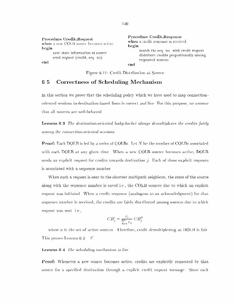
140
Procedure Credit Request
when a new COLB source becomes activebegin
save state information at sourcesend request (credit, seq. no)
end
Procedure Credit Response
when a credit response is receivedbegin
match the seq. no. with credit requestdistribute credits proportionally amongrequested sources
end
Figure 6.11: Credit Distribution at Source
6.5 Correctness of Scheduling Mechanism
In this section we prove that the scheduling policy which we have used to map connection-
oriented sessions to destination-based ows is correct and live. For this purpose, we assume
that all sources are well-behaved.
Lemma 6.3 The destination-oriented leaky-bucket always demultiplexes the credits fairly
among the connection-oriented sessions.
Proof: Each DOLB is fed by a series of COLBs. Let N be the number of COLBs associated
with each DOLB at any given time. When a new COLB source becomes active, DOLB
sends an explicit request for credits towards destination j. Each of these explicit requests
is associated with a sequence number.
When such a request is sent to the shortest multipath neighbors, the state of the source
along with the sequence number is saved i.e., the COLB sources due to which an explicit
request was initiated. When a credit response (analogous to an acknowledgment) for that
sequence number is received, the credits are fairly distributed among sources due to which
request was sent. i.e.,
CRij =
riPa ra
CRSj
where a is the set of active sources. Therefore, credit demultiplexing at DOLB is fair.
This proves Lemma 6.3. 2
Lemma 6.4 The scheduling mechanism is live.
Proof: Whenever a new source becomes active, credits are explicitly requested by that
source for a speci�ed destination through a explicit credit request message. Since each

141
of these messages are associated with a sequence number, according to Lemma 6.3, when
the source receives a credit response, credits are assigned proportionally to all requested
sources. In the worst case, a credit request might have to go all the way up to the destination
before it gets desired allocation. Since in steady state, we maintain loop-free paths to all
destinations, the hop-count from source to a destination is �nite.
Therefore, the scheduling mechanism is live. This proves Lemma 6.4. 2
Theorem 8 The scheduling mechanism is correct.
Proof: Lemma 6.3 and 6.4 ensure that the scheduling mechanism will not have any dead-
locks and all the active sources have a fair share of the available credits at all times. This
proves theorem 8. 2
6.6 Supporting Subnets
Having de�ned the basic protocol to support several QoS types in a packet-switched network,
we extend it to larger networks with hierarchical topologies in order to make the protocol
scalable.
6.6.1 Credit Aggregation
Destination-oriented credits are aggregated at all intermediate nodes from destination to-
wards source. Therefore, a credit value at each hop gives the total credits available to a
speci�ed destination through all the feasible paths through its downstream nodes.
For the purpose of credit aggregation, we assume that the sources are well-behaved. Let
us assume that the network is divided into clusters. Each cluster is viewed as a single entity
from any node outside the cluster. All the information (distribution of credits) within the
cluster is transparent to the nodes outside the cluster. The border node at each cluster is
responsible for sending aggregated credit information to all the nodes/clusters outside its
own cluster and then to distribute the credits fairly among the routers within the cluster.
Available credits are aggregated for each destination (cluster) at all routers (boundary
nodes) along the path from a destination to a source. When a source becomes active, it sends

142
B
S1 S2
D1D2
D
A
Figure 6.12: Credit Aggregation
an explicit credit request towards the desired destination. Destination in turn redistributes
credits (reserving resources along the way). The number of packets entering the network is
controlled at the COLB sources itself. Because of this, the sources cannot misbehave and
hog the resources allocated for other sources. The COLB sources are not allowed to send
data unless we have credits to do so. This ensures that the sources will not misbehave.
Because of the well-behavior of the sources, we can aggregate the available credits for
destinations. This can be done without maintaining any additional information about the
subnetworks. i.e., the topology of the subnetwork is transparent to the routers outside the
subnetwork. Therefore, the credit-based approach is scalable.
Figure 6.12 shows an example of how the credits are aggregated in a subnet. S1 and
S2 are the two sources and D1 and D2 are the two destination for which the sources are
sending data. The solid line indicates the direction of the data ow and the dashed line
indicates the direction of the credit ow. But, from the point of view of the two sources, the
information about both the destination have been integrated into a single destination D,
which is the boundary node of the destination cluster. D aggregates the credits available
for the two destinations within its cluster and passes on that information towards sources
S1 and S2.
143
Because the sources are well behaved and cannot send data to the destination unless
they have credits to do so, the credits obtained are distributed between the two sources in
proportion to their tra�c arrival rate.
6.6.2 Fairness
Fairness can be de�ned as two sources of the same capacity (arrival rate), destined for
the same destination and having the same QoS requirement get an equal share of the
bandwidth. Fairness can be ensured in the proposed destination oriented credit mechanism
among all active destinations as all destinations are served according to the tra�c rate
using a weighted fair queueing scheme at all nodes. The available credit is distributed
among active destinations in proportions relative to their tra�c arrival rate. Furthermore,
the congestion control scheme is exercised hop-by-hop on a per destination basis, so that
the congestion ow for one destination do not block the ows for other destinations.
At each hop, credits are allocated to ows depending on its relative input tra�c rate
into that node. Because the sources can not pump packets into the network unless they
have credits to do so (sources are well behaved), all sources get a fair share of the available
bandwidth.
6.7 Summary
In this chapter, we have proposed a new approach for combining routing and congestion
control in a packet-switched network. Our protocol is based on hop-by-hop credit distri-
bution and a loop-free multipath routing algorithm based on LPA. The new framework
dynamically adapts to congestion so that the entries in the routing tables re ect the state
of the network at any given time. We have demonstrated that it is possible to provide some
performance bounds for the delivery of packets in such networks. A two-tier architecture
to support end-to-end connections on top of a connectionless architecture is also presented
to support several levels of quality of service. We have also showed that it is possible to
extend this solution to a large networks. Our protocol guarantees that in the proposed

144
two-tier architecture, all packets that enter the connectionless network will be delivered to
their respective destinations unless a resource failure prevents it.

145
Chapter 7
Summary and Future Work
This dissertation addresses the design and analysis of routing algorithms and protocols
for packet-switched networks. We identi�ed the basic drawbacks of the existing routing
techniques and also identi�ed the requirements for new applications, which include wire-
less communication as well as wired applications. Di�erent types of routing protocols are
required in the network in order to support these diverse requirements. Low protocol over-
head, scalability and ability to quickly adapt to the dynamic state of the network are some
of the issues to be concerned about. In some cases, data tra�c or best-e�ort tra�c, does
not su�ce the application requirements. The main objective of this dissertation has been
to take advantage of the application requirements and to propose an appropriate loop-free
routing protocol.
The performance of an application can be improved by correctly designing a routing
algorithm and thereby minimizing the protocol overhead. It is thus necessary to identify
the application requirements for a correct design of the routing algorithm. It is also a fact
that the performance of routing algorithms is greatly a�ected by the congestion control
and the feedback mechanism of the system. For this reason, we integrate both congestion
control and routing functions in one of our proposals.
We have formally veri�ed our proposals, proving the algorithms to be correct and loop-
free when applicable and have analyzed the complexity of the algorithms. We have also
obtained a worst-case delay bound on the congestion oriented protocol using analytical
techniques. For most of our proposals, the performance of the routing algorithms has been

146
evaluated by means of simulations. Simulations were performed using a C-based routing
simulator called Drama. Well known topologies such as Los-Nettos, Nsfnet and Arpanet
were used in most of the simulations. To simulate our hierarchical routing algorithm, we
have used the modi�ed Doe-Esnet topology and a randomly generated topology with more
then 100 nodes.
7.1 New Path-Finding Algorithms
Two new routing algorithms, PFA and LPA, which belong to the class of path-�nding
algorithms have been proposed. These algorithms reduce the possibility of formation of
temporary routing loops. This is due to an e�cient updating mechanism and the usage of
implicit path information which can be extracted from the router's database maintained at
each node. LPA achieves loop-freedom at every instant using a single-hop inter-neighbor
coordination mechanism.
7.2 Hierarchical Routing Algorithm
The basic path-�nding algorithms for at networks have been extended to large, hierarchi-
cal networks to make the algorithms scalable. Here, the concept of maintaining predecessor
information for the paths to achieve loop-free paths has been extended across the global net-
work. This scheme ensures that the topological details within each subnet are transparent
to all nodes outside the subnetwork and we achieve loop free paths across the subnetworks.
This property makes the hierarchical routing algorithm scalable. Only one entry per sub-
network and the detailed information about all the nodes within the local subnet needs to
be maintained at each node. This technique can be used in the Internet to increase the
scalability of routing algorithms.
7.3 Wireless Routing Protocol
The requirements of a wireless network are very di�erent from a wireline network mainly due
to the limitation in the available bandwidth. WRP is a routing protocol that is suitable in a

147
wireless environment and which takes into account the constraints of a wireless environment.
This is a simple protocol which does not need any elaborate synchronization mechanism and
has fast convergence properties. To limit the number of routing control messages exchanged
between nodes, we suggest some optimization techniques. WRP is shown to perform better
than state of the art routing protocols in wireless networks through simulations.
7.4 Congestion-Oriented Routing
Providing Quality-of-Service (QoS) guarantees in packet-switched networks places stringent
demands on the underlying system. It is a well known that congestion control and routing
are interrelated problems. We propose a technique to combine routing and congestion
control functions and provide a multipath solution to the above problem. Worst-case delay
bounds have been provided using analytical techniques. This model provides ow isolation
because of the PGPS scheduling scheme used at each node. To support the quality of service
required by the applications in a packet-switched environment, a two-tier architecture has
been de�ned wherein a connection-oriented session sits on top of a packet-switched ow. A
credit based protocol is used to ensure guaranteed ows within the packet-switched network
and a scheduling mechanism is used to map connection-oriented sessions to packet-switched
ows. The correctness of both the credit-based mechanism and the scheduling scheme have
been proved analytically.
7.5 Future Work
Routing Information Protocol (RIP) [Hed88] is still the most widely used intra-domain
routing protocol. Like many other protocols, RIP is also based on Distributed Bellman-
Ford algorithm (DBF) for shortest path computations. To cope with the counting-to-in�nity
problems of DBF, the longest path in RIP is limited to 15 hops. Recently, RIP version
2 [Mal94] has been proposed, which adds more information to RIP and reports the next
hop information in the routing updates. However, this still does not prevent the counting-to-
in�nity problem. However, the format of RIP version 2 permits the speci�cation of limited

148
path information. Our work can be extended to propose a new Internet routing protocol,
which overcomes the drawbacks of RIP using the same packet format at RIP version 2.
The integration of congestion control and routing is an important result since the routing
tables entries can be used to de�ne long term connections along the non-congested paths.
This proposal uses a multipath routing algorithm. An immediate extension of this work
will be to study the behavior of multicast connections and combining it with congestion
control issues to de�ne long-term multicast sessions.
Another extension is to study the mobility issues in conjunction with wireless routing.
Issues such as hierarchical clustering and hand-o�s needs to be addressed. In addition to
this, we can introduce another level of complexity in the study by providing guaranteed
ows based on application requirements (issue of QoS).
Finally, the scheduling mechanism that is used to map connection-oriented sessions to
packet-switched ows can be a topic of further research.
Some work is also being done in securing distance-vector routing protocols. [SMGLA96]
gives the details of this protocol.
149
Bibliography
[Ana96] Arul Ananthanarayanan. Implementation of path-�nding routing algorithmsfor unix. Master's thesis, San Diego State University, 1996.
[Bea89] D. Beyer and et. al. Packet radio network research, development and ap-plication. In Proceedings SHAPE conference on Packet Radio, Amesterdam,1989.
[Bel57] R.E. Bellman. Dynamic Programming. Princeton University Press, Prince-ton, N.J., 1957.
[Ber82] D. Bertsekas. Dynamic behavior of shortest path routing algorithms. IEEETrans. Automatic Control, AC-27:60{74, 1982.
[Bey90] D. Beyer. Accomplishments of the DARPA SURAN program. In MILCOM,pages 855{862, Monterey, California, Dec. 1990. IEEE.
[BG92] D. Bertsekas and R. Gallager. Data Networks. Prentice-Hall Inc, 2nd edition,1992.
[BJ83] A.E. Baratz and J.M. Ja�e. Establishing virtual circuits in large computernetwroks. In INFOCOM, pages 311{318, San Diego, CA, April 1983. IEEE.
[CE95] M. Scott Corson and Anthony Ephremides. A distributed routing algorithmfor mobile wireless networks. ACM J. Wireless Networks, pages 61{81, Jan.1995.
[Ceg75] T. Cegrell. A routing procedure for the TIDAS message switching network.IEEE Trans. Commun., 23(6):575{585, 1975.
[CRKGLA89] C. Cheng, R. Reley, S.P.R. Kumar, and J.J. Garcia-Luna-Aceves. A loop-freeextended bellman-ford routing protocol without bouncing e�ect. In Com-puter Communications Review, volume 19, pages 224{236. ACM, 1989.
[Cru91] R.L. Cruz. A calculus for network delay, part II: Network analysis. IEEETrans. Information Theory, 37:132{141, 1991.

150
[DH96] S. Deering and R. Hinden. Internet protocol, version 6 (ipv6) speci�cation.RFC 1883, Jan. 1996.
[DS80] E.W. Dijkstra and C.S. Scholten. Termination detection for di�using com-putations. In Information Processing Letters, volume 11. 1980.
[Far93] Dino Farinacci. Introduction to enhanced IGRP. Cisco Systems, June 1993.
[FJ94] S. Floyd and V. Jacobson. The synchronization of periodic routing messages.IEEE/ACM Trans. Networking, 2(2):122{136, April 1994.
[GLA] J.J. Garcia-Luna-Aceves. A minimum-hop routing algorithm based on dis-tributed information. Computer Networks and ISDN Systems, 16:367{382.
[GLA86] J.J. Garcia-Luna-Aceves. A fail-safe routing algorithm for multihop packetradio networks. In INFOCOM, Maiami, Florida, April 1986. IEEE.
[GLA92a] J.J. Garcia-Luna-Aceves. Distributed routing with labeled distances. InINFOCOM, pages 633{643. IEEE, 1992.
[GLA92b] J.J. Garcia-Luna-Aceves. Libra: A distributed routing algorithm for largeinternets. In GLOBECOM, volume 3, pages 1465{1471. IEEE, Dec. 1992.
[GLAM95] J.J. Garcia-Luna-Aceves and Shree Murthy. A loop-free path-�nding algo-rithm: Speci�cation, veri�cation and complexity. In INFOCOM, Boston,April 1995. IEEE.
[GLAM96] J.J. Garcia-Luna-Aceves and Shree Murthy. A path-�nding algorithm forloop-free routing. IEEE/ACM Trans. Networking, 1996. to appear in.
[GLAS85] J.J. Garcia-Luna-Aceves and N. Shacham. Analysis of routing strategiesfor packet radio networks. In INFOCOM, pages 292{302, Washington D.C.,March 1985. IEEE.
[GLAZ94] J.J. Garcia-Luna-Aceves and William T. Zaumen. Area-based loop-free in-ternet routing. In INFOCOM, volume 3, pages 1000{1008, Toronto, Canada,April 1994. IEEE.
[Hag83] J. Hagouel. Issues in routing for large dynamic networks. Technical Report9942 (No. 44055, IBM Research Report, April 1983.
[Hed] Charles Hedrick. An introduction to IGRP. Rutgers University.
[Hed88] C. Hedrick. Routing information protocol. RFC 1058, June 1988.
[HS82] R. Hinden and A. Sheltzer. DARPA internet gateway. RFC 823, Sept. 1982.
[Hui95] Christian Huitema. Routing in the Internet. Prentice Hall, 1995.
[Hum91] P.A. Humblet. Another adaptive shortest-path algorithm. IEEE Trans.Commun., 39(6):995{1003, June 1991.

151
[Jaf88] J.M. Ja�e. Hierarchical clustering with topology databases. Computer Net-works and ISDN Systems, 15:329{339, 1988.
[JM82] J.M. Ja�e and F.M. Moss. A responsive routing algorithm for computernetworks. IEEE Trans. Commun., 30:1758{1762, July 1982.
[Kam76] F. Kamoun. Design Considerations for Large Computer CommunicationsNetwork. PhD thesis, University of California, Santa Cruz, 1976. UCLA-ENG-7642, Computer Science Dept.
[KTA94] H.T Kung, Blackwell. T, and Chapman. A. Credit-based ow control forATM networks: credit update protocol, adaptive credit allocation, and sta-tistical multiplexing. In ACM SIGCOMM, volume 24 of CCR, pages 101{14,London, UK, Aug/Sept 1994. ACM.
[Lau86] G.S. Lauer. Hierarchical routing design for suran. In ICC, pages 4.2.1{4.2.10,Toronto, Canada, June 1986. IEEE.
[LNT87] B.M. Leiner, D.L. Nielson, and F.A. Tobagi. Issues in packet-radio networkdesign. volume 75 of Proc. of IEEE, pages 6{20, Jan. 1987.
[Mal94] G. Malkin. RIP version 2: Carrying additional information. RFC 1723, Nov.1994.
[McQ74] J. McQuillan. Adaptive routing algorithms for distributed computer net-works. Technical report, Bolt Beranek and Newman, 1974.
[MGLA94] Shree Murthy and J.J. Garcia-Luna-Aceves. A more e�cient path-�ndingalgorithm. In 28th Asilomar Conference, pages 229{233, Paci�c Groove,California, Nov. 1994.
[MGLA95] Shree Murthy and J.J. Garcia-Luna-Aceves. A routing protocol for packet-radio networks. In Mobile Computing and Networking Conference, Berkeley,CA, Nov. 1995. ACM.
[MGLA96] Shree Murthy and J.J. Garcia-Luna-Aceves. A routing protocol for wirelessnetworks. Mobile Networks and Applications, 1(2), 1996. Special Issue onRouting in Mobile Communications Network.
[Mil83a] D. Mills. DCN local network protocols. RFC 891, Dec. 1983.
[Mil83b] D. Mills. Exterior gateway protocol. RFC 904, Dec. 1983.
[Moy94] J. Moy. OSPF version 2. RFC 1583, March 1994.
[MRR78] J.M. McQuillan, I. Richer, and E.C. Rosen. Arpanet routing algorithm im-provements. Technical Report 3803, BBN, April 1978.
[MRR80] J. McQuillan, I. Richer, and E. Rosen. The new routing algorithm for theArpanet. IEEE Trans. on Commun., COM-28(5):711{19, May 1980.

152
[MS79] P.M. Meerlin and A. Segall. A failsafe distributed routing algorithm. IEEETrans. Commun., 27:1280{1288, Sept. 1979.
[Mur94] Shree Murthy. Design and analysis of distributed routing algorithms. Mas-ter's thesis, University of California, Santa Cruz, June 1994.
[MW77] J. McQuillan and D.C. Walden. The ARPANET design decisions. ComputerNetworks, 1, Aug. 1977.
[Ora90] D. Oran. OSI IS-IS intra-domain routing protocol. RFC 1247, Feb. 1990.
[OSV94] C. Ozveren, R. Simcoe, and G. Varghese. Reliable and e�cient hop-by-hop ow control. In SIGCOMM, pages 89{110, London, Aug/Sept. 1994.
[PB94] Charles E. Perkins and Pravin Bhagwat. Highly dynamic destination-sequenced distance-vector routing (DSDV) for mobile computers. In SIG-COMM, pages 234{244. ACM, 1994.
[Per91] Radia Perlman. A comparison between two routing protocols: OSPF andIS-IS. In IEEE Network, volume 5, pages 18{24, Sept. 1991.
[PG93] A.K. Parekh and R.G. Gallager. A generalized processor sharing ap-proach to ow control in integrated services networks: The single-node case.IEEE/ACM Trans. Networking, 1(3):344{357, June 1993.
[PG94] A.K. Parekh and R.G. Gallager. A generalized processor sharing approachto ow control in integrated services networks: The multiple node case.IEEE/ACM Trans. Networking, 2(2):137{150, April 1994.
[RF91] B. Rajagopalan and M. Faiman. A responsive distributed shortest-path rout-ing algorithm within autonomous systems. Internetworking: Research andExperience, 2(1):51{69, March 1991.
[RL94] Y. Rekhter and T. Li. Border gateway protocol 4 (BGP-4). RFC, Jan. 1994.
[RT83] C.V. Ramamoorthy and W. Tsai. An adaptive hierarchical routing algorithm.In COMPSAC, pages 93{104. IEEE, Nov. 1983.
[Sch86] M. Schwartz. Telecommunications Networks: Protocols, Modeling and Anal-ysis. Addison-Wesley Publishing Co.,, Menlo Park, California, 1986. Chapter6.
[SK86] J. Seeger and A. Khanna. Reducing routing overhead in a growing DDN. InMILCOM, volume 1, pages 15.3.1{15.3.13. IEEE, Oct. 1986.
[SMGLA96] Brad Smith, Shree Murthy, and J.J. Garcia-Luna-Aceves. Securing distance-vector routing protocols. UCSC Technical Report, 1996.
[Tan91] Andrew S. Tanenbaum. Computer Networks. Prentice Hall, second edition,1991.

153
[Wax88] B.M. Waxman. Routing of multipoint connections. J. Selected Areas inCommun., 6(9):1617{1622, 1988.
[Zau91] W.T. Zaumen. Simulations in drama. Network Information System Center,SRI International, Jan. 1991.
[ZDE+93] Lixia Zhang, Steve Deering, Deborah Estrin, Scott Shenker, and Daniel Zap-pala. Rsvp: A new resource reservation protocol. In Network Magazine,volume 7, pages 8{18. IEEE, Sept. 1993.
[ZGLA92] W.T. Zaumen and J.J. Garcia-Luna-Aceves. Dynamics of link-state andloop-free distance-vector routing algorithms. In Internetworking: Researchand Experience, volume 3, pages 161{188. 1992.
Recommended