ORC: An Online Competitive Algorithm for Recommendationand Charging Schedule in Electric Vehicle Charging Network
Bo Sun
The Hong Kong University of Science
and Technology
Tongxin Li, Steven H. Low
California Institute of Technology
{tongxin,slow}@caltech.edu
Danny H.K. Tsang
The Hong Kong University of Science
and Technology
ABSTRACTThere is an increasing need for spatial and temporal schedule tai-
lored to the requests and preferences of electric vehicles (EVs) in a
network of charging stations. From the perspective of a charging
network operator, this paper considers an online decision-making
problem that recommends charging stations and the corresponding
energy prices to sequential EV arrivals, and schedules the charging
allocation to maximize the expected total revenue. To address the
uncertainties from future EV arrivals and EVs’ choices with respec-
tive to recommendations, we propose an Online Recommendation
and Charging schedule algorithm (ORC) that is parameterized by
a value function for customized designs. Under the competitive
analysis framework, we provide a sufficient condition on the value
function that can guarantee ORC to be online competitive. More-
over, we design a customized value function based on the sufficient
conditions in an asymptotic case, and then rigorously prove the
competitive ratio of ORC in the general case. Through extensive
experiments, we show that ORC achieves significant increase of
revenues compared to benchmark online algorithms.
CCS CONCEPTS• Theory of computation → Online algorithms; • Networks→ Network economics.
KEYWORDSElectric vehicles, online algorithms, recommendation, charging
schedule, competitive ratios
ACM Reference Format:Bo Sun, Tongxin Li, Steven H. Low, and Danny H.K. Tsang. 2020. ORC: An
Online Competitive Algorithm for Recommendation and Charging Schedule
in Electric Vehicle Charging Network. In The Eleventh ACM InternationalConference on Future Energy Systems (e-Energy’20), June 22–26, 2020, VirtualEvent, Australia. ACM, New York, NY, USA, 12 pages. https://doi.org/10.
1145/3396851.3397727
1 INTRODUCTIONMobility and energy management of a population of electric ve-
hicles (EVs) have drawn great attention from both industry and
Permission to make digital or hard copies of all or part of this work for personal or
classroom use is granted without fee provided that copies are not made or distributed
for profit or commercial advantage and that copies bear this notice and the full citation
on the first page. Copyrights for components of this work owned by others than ACM
must be honored. Abstracting with credit is permitted. To copy otherwise, or republish,
to post on servers or to redistribute to lists, requires prior specific permission and/or a
fee. Request permissions from [email protected].
e-Energy’20, June 22–26, 2020, Virtual Event, Australia© 2020 Association for Computing Machinery.
ACM ISBN 978-1-4503-8009-6/20/06. . . $15.00
https://doi.org/10.1145/3396851.3397727
academy with the increasing penetration of EVs in both public
(e.g., EV buses/taxis) and private transportation [10, 13, 20, 25]. For
a charging network operator (CNO) who manages multiple pub-
licly accessible charging stations, two types of decisions need to
be made upon the arrival of each EV: (i). A spatial schedule thatdecides which station the EV should be assigned/recommended to
and (ii). A temporal schedule that determines when the EV should be
charged at the station decided by the spatial schedule. The follow-
ing three practical issues arise for a CNO to solve this sequential
decision-making problem.
• Uncertainty, it is challenging to predict the charging de-
mand (such as energy to be delivered and its deadline) of
each EV since it varies with time, location, and the state of
each individual EV (e.g., state-of-charge and battery capac-
ity) [1, 19, 24]. A CNO needs to design an online algorithmthat makes spatial and temporal schedules without knowing
the information of future arrivals.
• Discretion, unlike managing an EV fleet owned by a private
operator, a CNO cannot assign the EVs to charging stations
by mandatory orders [10, 13]. One promising solution is
to strategically devise a charging offer, which contains a
recommended charging station and a corresponding energy
price, for each EV to choose by itself. EVs can choose to
accept this offer, or reject it and leave for alternative charging
facilities.
• Commitment, the charging demand is time-varying and
geographically unbalanced. As a result, the states of charg-
ing stations (e.g., number of idle chargers) at the time when
a CNO recommends stations may differ from when an EV ar-
rives at the station for charging. Consequently, the demands
of EVs may not be satisfied. To guarantee the quality of ser-
vice, when making spatial schedules, a CNO needs to make
on-arrival commitment [1], by reserving enough charging
capacity for future temporal schedules.
In consideration of the three issues above, the key challenge of
designing and analyzing an online algorithm lies in making deci-
sions with two types of uncertainties. Type I uncertainty includes
the charging demands and contextual information (e.g., location,
time, EV brand, etc.) of all future EVs. Type II uncertainty is the
randomness that EVs may or may not accept the recommendations
provided by a CNO. Note that EVs may choose to reject all recom-
mendations and no revenues can be achieved by both online and
offline algorithms. Therefore, instead of focusing on the worst-case
scenario for both Type I and II uncertainties, it is desirable to have a
less conservative online algorithm that maximizes the expected to-
tal revenue averaging over all Type II realizations in the worse-case
realization of Type I uncertainty.
144

e-Energy’20, June 22–26, 2020, Virtual Event, Australia B. Sun, T. Li, S.H. Low, and D.H.K. Tsang
Contributions. In this paper, based on a recommender system
formed by a CNO and a network of charging stations, we design
an Online algorithm that decides Recommendations and Chargingschedules with on-arrival commitment (ORC) for sequential EVarrivals. In more detail, an EV initiates a charging session inquiry,
which includes its energy demand and charging deadline, to a CNO
through an online platform. Upon receiving the inquiry, an ORCoffers that EV a station-price pair, which indicates the energy price
if the EV charges at this station. This offer can also be set as an
empty entry if no charging station is available. The EV then decides
whether to accept it or not. If the recommendation is accepted, the
EV will arrive at the recommended station and pay for the charging
service with the fixed price in the offer. If the EV rejects the offer,
it can either leave for alternative charging facilities, or adjust its
charging demand (by reducing its energy demand or extending its
departure time) and submit a new inquiry, which may be offered a
more satisfactory recommendation. For each accepted offer, anORCmanages to schedule charging that satisfies the EV’s demand, i.e.,
to deliver the required energy by the deadline at the recommended
charging station. The objective of an ORC is to maximize the total
revenue collected from all EVs.
Value functions (see Definition 3.1) that evaluate the marginal
cost for charging an EV at a given charging station are used to
parameterize the ORC. As our next result, in Theorem 4.2, we
provide a sufficient condition on value functions for ensuring that
the ORC has a constant (expected) competitive ratio. Furthermore,
based on the sufficient condition, we propose a systematic way for
generating an explicit value function with a provable competitive
ratio summarized in Theorem 4.4.
To demonstrate the effectiveness of the ORC, we provide a case-study based on geographical data in Hong Kong in Section 6. The
(empirical) competitive ratios in our experiments outperform other
three online benchmarks.
Related work. A rich literature on online management of EVs
has emerged in recent years and the work can be broadly divided
into two branches. In the sequel, we overview a collection of the
representative results.
Temporal scheduling of EVs. The key idea in temporal scheduling
of EVs is treating the EVs as deferrable loads and schedule the
charging based on their demands. Along the lines of this idea,
previous work has been focusing on coordinating the charging
process of a fleet of EVs by temporal load shifting (i.e., temporal
schedules) to mitigate their negative impacts on power systems [6,
7] or gain profits [19, 21]. Online algorithms have been considered
in [1–3, 9, 9, 19, 23], which aim to achieve a bounded competitive
ratio. Some recent work [15, 17, 24] developed auction-based or
posted price mechanisms to handle the EVs’ choices but the main
focus there is temporal scheduling for a single charging station.
The authors of [1] reported an impossibility result that there is no
competitive online algorithm for on-arrival commitment charging
schedule in the general setting. However, this paper will show
that our proposed online algorithm ORC can achieve a bounded
competitive ratio if more information (e.g., the set of possible prices
and the choice probabilities of EVs) is given for decision-making.
Spatial scheduling of EVs. More recent studies [4, 20, 25] indicate
that it is also of great importance to recognize EVs as mobile loads,
which can be scheduled to be served at different locations (i.e.,
spatial schedules) to balance the location-dependent EV charging
demands. The literature on the spatial scheduling of EVs mainly
considers evaluating the system-level benefits of the spatial sched-
uling. For example, the authors of [4] designed a pricing strategy for
routing EVs to charging stations that optimizes the charging loads
of different nodes in a transmission network and simultaneously
mitigates the congestion of a transportation network. The authors
of [25] used a game-theoretic approach to devise a spatial-temporal
scheduling formultiple groups of public EVs competing for capacity-
limited charging stations. Further investigations on pricing mecha-
nisms for private EVs that charge at public EV charging stations can
be found in [13]. Although geographical information is considered,
most existing works on spatial scheduling model EV arrivals as a
stationary distribution that is known a priori. In contrast to this, re-
alistic EV arrival patterns depend on times and locations and are in
general hard to forecast [1, 19, 24]. Designing an online algorithm
for spatial scheduling with sequential EV arrivals is therefore still
an open and challenging task. There is a theory-to-application gap
between existing online algorithms mainly designed for temporal
scheduling and practical situations wherein EVs are spatial loads
and have their own freedom to make decisions. The main goal of
this paper is to close this gap by proposing an online competitive
algorithm for joint spatial and temporal scheduling.
2 PROBLEM STATEMENTThis section first presents the online spatial-temporal scheduling
problem that an ORC solves. Next, we formally define the expected
competitive ratio, as an offline benchmark and then an auxiliary
optimization is given whose optimal value bounds the expected
competitive ratio from above, based on which the ORC is designed
and analyzed.
2.1 Online spatial-temporal schedulingThe CNO manages a set M := {1, . . . , 𝑀} of geographically dis-
tributed charging stations. Each charging station𝑚 ∈ M is equipped
with 𝑏𝑚 chargers, each of which can be used for on/off charging
control with a fixed charging rate 𝑅𝑚 . Due to varying electricity
prices, each station𝑚 ∈ M is allowed to set their energy prices
for charging sessions from a set of price levels R𝑚 := {𝑟𝑚,𝑗 }𝑗 ∈J𝑚 ,
where J𝑚:= {1, . . . , 𝐽𝑚} is the index set of price levels. Without
loss of generality, the price levels are sorted in an ascending order,
i.e., 0 < 𝑟𝑚,1 < · · · < 𝑟𝑚,𝐽𝑚.
A set N := {1, . . . , 𝑁 } of EVs sequentially submit charging ses-
sions to the CNO. Consider a time-slotted system1indexed by
𝑡 ∈ T := {1, . . . ,𝑇 } with a fixed slot length Δ𝑇 . Let 𝑎𝑛 , 𝑒𝑛 , and 𝑑𝑛denote the submission time, energy demand, and deadline of charg-
ing session 𝑛, respectively. To model EVs’ preferences for stations
and prices, we define the following matrix of probabilies.
Choice probabilities. Based on the charging requests and con-
textual information, we assume each EV has a fixed choice proba-bility over the recommended station-price pairs. The choice prob-
ability of EV 𝑛 is denoted by 𝒑𝑛 := {𝑝𝑚,𝑗𝑛 }𝑚∈M, 𝑗 ∈J𝑚 where 𝑝
𝑚,𝑗𝑛
indicates the preference of an EV 𝑛 for charging at station𝑚 with
1Charging sessions can be submitted and processed in real time but the charging
schedule has to be done over discrete time steps.
145
ORC: An Online Competitive Algorithm for Recommendationand Charging Schedule in Electric Vehicle Charging Network e-Energy’20, June 22–26, 2020, Virtual Event, Australia
the price 𝑟𝑚,𝑗. It must satisfy that (i) 0 ≤ 𝑝
𝑚,𝑗𝑛 ≤ 1, and (ii) it is mono-
tonically non-increasing with respect to price, i.e., 𝑝𝑚,𝑗𝑛 ≤ 𝑝
𝑚,𝑗 ′𝑛 for
all 𝑗 ′ < 𝑗 and𝑚 ∈ M.
Upon the submission of an EV 𝑛 ∈ N , the CNO has access to the
following information:
• Charging requirements of an EV 𝑛 in different charging
stations {𝑒𝑛,𝑚,T𝑛,𝑚}𝑚∈M , where 𝑒𝑛,𝑚 = ⌈𝑒𝑛/(𝑅𝑚Δ𝑇 )⌉ is
the required number of time slots to charge EV 𝑛 at station
𝑚 and T𝑛,𝑚 := {𝑎𝑛 + 𝑡𝑛,𝑚, . . . , 𝑑𝑛} is the set of feasible time
slots for charging EV 𝑛 at station𝑚, where 𝑡𝑛,𝑚 denotes the
estimated traveling time for EV 𝑛 to reach station𝑚.
• The matrix of probabilities 𝒑𝑛 .
The CNO then performs spatial scheduling (i.e, deciding a station-
price recommendation) based on the above information and tempo-
ral scheduling (i.e, allocating charging time slots) for each charging
session. In the following, we introduce more decision variables that
the CNO can optimize over to maximize its revenue.
Recommendation decisions. The recommendation variable𝑦𝑚,𝑗𝑛 ∈ {0, 1} is one if a station-price pair (𝑚, 𝑗) is recommended
to an EV 𝑛 and zero otherwise. No recommendation will be made
if 𝑦𝑚,𝑗𝑛 = 0 for all𝑚 ∈ M and 𝑗 ∈ J𝑚
. For the simplicity of pre-
sentation and analysis, we assume each EV 𝑛 only received one
recommendation and our proposed scheme can be easily extended
to the cases when multiple recommendations are given to each EV.
Charging decisions. Another binary variable 𝑥𝑚,𝑗𝑛,𝑡 ∈ {0, 1} is
the charging variable that determines whether to charge an EV 𝑛 at
station𝑚 ∈ M at time 𝑡 ∈ T𝑛,𝑚 . Again, for the ease of presentation,
we restrict the charging levels to be two-states–on and off.
Maximization objective. Given a recommended station-price
pair (𝑚, 𝑗), if an EV 𝑛 accepts this offer, it pays 𝑒𝑛𝑟𝑚,𝑗
to the CNO
and drives to station𝑚 for charging. The CNO guarantees to deliver
𝑒𝑛 energy to this EV before its deadline𝑑𝑛 at station𝑚. The objective
of the CNO is to maximize the total revenue collected from all EVs.
After receiving the recommendation pair, the EV 𝑛 accepts it
with probability 𝑝𝑚,𝑗𝑛 .
Remark 2.1. When choice probabilities are all ones, the spatial
decision of the online problem reduces to an assignment problem
as EVs will accept any recommendation for sure.
Remark 2.2. (An example of estimating choice probabilities) We
can model the preference of EV 𝑛 over station-price pair (𝑚, 𝑗) as𝑓𝑛 (𝑚, 𝑗 ;𝜸𝑛) = 𝛾𝑛 (1) + 𝛾𝑛 (2)/𝑡𝑛,𝑚 + 𝛾𝑛 (3)/(𝑟𝑚,𝑗 )2,
which is inversely proportional to the driving time to station𝑚 and
the energy price 𝑟𝑚,𝑗. 𝜸𝑛 = [𝛾𝑛 (1), 𝛾𝑛 (2), 𝛾𝑛 (3)] customizes the
preference of each EV 𝑛 and can be estimated from historical data
by regression. The choice probability of EV 𝑛 for the station-price
pair (𝑚, 𝑗) can be estimated by a softmax function:
𝑝𝑚,𝑗𝑛 =
exp
(𝑓𝑛 (𝑚, 𝑗 ;𝜸𝑛)
)∑𝑚∈M
∑𝑗 ∈J𝑚 exp
(𝑓𝑛 (𝑚, 𝑗 ;𝜸𝑛)
) . (1)
An instance of the online spatial-temporal schedule problem
contains three types of information:
• Setup information S := {M, {𝑏𝑚}𝑚∈M , {R𝑚}𝑚∈M };
• Arrival information I := {𝜽𝑛}𝑛∈N , where the arrival infor-
mation of EV 𝑛 is 𝜽𝑛 = {{𝑒𝑛,𝑚,T𝑛,𝑚}𝑚∈M ,𝒑𝑛};
• Choice information W := {𝒘𝑛}𝑛∈N , where the choice in-
formation of EV 𝑛 is 𝒘𝑛 := {𝑤𝑚,𝑗𝑛 }𝑚∈M, 𝑗 ∈J𝑚 , in which
𝑤𝑚,𝑗𝑛 ∈ {0, 1} is EV 𝑛’s choice on the recommendation (𝑚, 𝑗)
where𝑤𝑚,𝑗𝑛 is a realization of the Bernoulli random variable
𝑊𝑚,𝑗𝑛 with success probability 𝑝
𝑚,𝑗𝑛 .
The setup information S is fixed and known by the CNO a priori
while the arrival information and choice information are revealed
sequentially, and especially, the choice information depends on pre-
vious decisions. Given a setup S, the goal in this paper is to design
an online algorithm operated by the CNO that generates station-
price recommendations for each EV 𝑛 and schedules charging based
on the arrival information 𝜽 1, . . . , 𝜽𝑛 and the choice information
𝒘1, . . . ,𝒘𝑛−1. We encode the information available at an online
CNO for providing a recommendation for an EV 𝑛 by
F𝑛 := {S, 𝜽 1, . . . , 𝜽𝑛,𝒘1, . . . ,𝒘𝑛−1}. (2)
Let ALG(I;W) denote the revenue collected from an online al-
gorithm for an arrival instance I. ALG(I;W) is a random vari-
able with respective to W, the random choices from EVs . The
goal of the online algorithm is to maximize the expected revenue
EW [ALG(I,W)].Next we define an offline benchmark for the online algorithm.
Let O𝑛 = F𝑛 ∪ {𝜽𝑛+1, . . . , 𝜽𝑁 } denote the offline information for
decision-making of EV 𝑛 given the entire arrival information I.In this offline benchmark, even though the choice probabilities of
all future EVs are known a priori, the realizations of future EVs’
choices, including the current one, are unknown for the offline
benchmark. Therefore, the optimal offline algorithm is an adaptive
algorithm and the optimal solution is a policy mapping the offline
information O𝑛 to decisions. Let 𝑌𝑚,𝑗𝑛 (O𝑛) and 𝑋𝑚,𝑗
𝑛,𝑡 (O𝑛) denotethe recommendation and charging variables based onO𝑛 .𝑌
𝑚,𝑗𝑛 (O𝑛)
and 𝑋𝑚,𝑗𝑛,𝑡 (O𝑛) are the outputs of a causal decision maker 𝜋 whose
decisions can only be made based on O𝑛 . The CNO can collect a
revenue 𝑒𝑛𝑟𝑚,𝑗
from EV 𝑛 only if the station-price pair (𝑚, 𝑗) isoffered to EV 𝑛 (i.e., 𝑌
𝑚,𝑗𝑛 (O𝑛) = 1) and meanwhile the EV accepts
this offer (i.e.,𝑊𝑚,𝑗𝑛 = 1). The total revenue is
RVN(𝜋,I;W) :=
𝑁∑𝑛=1
𝑀∑𝑚=1
𝐽𝑚∑𝑗=1
(𝑒𝑛𝑟𝑚,𝑗 ) · 𝑌𝑚,𝑗𝑛 (O𝑛) ·𝑊𝑚,𝑗
𝑛 ,
subject to ∑𝑡 ∈T𝑛,𝑚
𝑋𝑚,𝑗𝑛,𝑡 (O𝑛) ≥ 𝑒𝑛,𝑚𝑌
𝑚,𝑗𝑛 (O𝑛), ∀𝑛,𝑚, 𝑗, (3a)
𝑁∑𝑛=1
𝐽𝑚∑𝑗=1
𝑊𝑚,𝑗𝑛 · 𝑋𝑚,𝑗
𝑛,𝑡 (O𝑛) ≤ 𝑏𝑚, ∀𝑚, 𝑡, (3b)
𝑀∑𝑚=1
𝐽𝑚∑𝑗=1
𝑌𝑚,𝑗𝑛 (O𝑛) ≤ 1, ∀𝑛, (3c)
𝑌𝑚,𝑗𝑛 (O𝑛) ∈ {0, 1}, ∀𝑛,𝑚, 𝑗, (3d)
𝑋𝑚,𝑗𝑛,𝑡 (O𝑛) ∈ {0, 1}, ∀𝑛,𝑚, 𝑗, 𝑡 ∈ T𝑛,𝑚, (3e)
where constraint (3a) is the energy constraint that ensures a charg-
ing allocation is scheduled to deliver 𝑒𝑛 amount of energy at station
𝑚 if EV 𝑛 is offered to charge at station𝑚. Constraint (3b) is the
146

e-Energy’20, June 22–26, 2020, Virtual Event, Australia B. Sun, T. Li, S.H. Low, and D.H.K. Tsang
capacity constraint ensuring the total number of EVs that are si-
multaneously charging at a station cannot exceed the total number
of chargers. Constraint (3c) restricts that at most one station-price
pair is offered to each EV. We consider the best causal decision
maker 𝜋∗ defined by
𝜋∗ = arg max
𝜋EW [RVN(𝜋,I;W)] . (4)
With 𝜋∗ being used, the optimal revenue for eachW isOPT(I;W)and the expectation EW [OPT(I;W)] is maximized.
Due to lacking future arrival information, any online algorithm
cannot achieve an expected offline revenue EW [OPT(I;W)]. Inthis paper, we aim to design an online algorithm that can achieve
at least a fraction of the offline revenue 𝛼EW [OPT(I;W)], where0 ≤ 𝛼 ≤ 1 is a constant and defined as the competitive ratio of the
online algorithm. Formally, the competitive ratio is defined as
𝛼 = min
all possible I
EW [ALG(I;W)]EW [OPT(I;W)] . (5)
The goal is to design an online algorithm that achieves a compet-
itive ratio as large as possible. Note that 𝛼 is defined as the ratio
of the expected revenues of the online and offline algorithms over
EVs’ random choices in the worse-case realization of EVs’ arrival
instances. Different from the conventional competitive analysis that
defines the ratio in the worse scenario regarding all uncertainties,
our expected competitive ratio is necessary in this problem since
EVs may reject all recommendations such that both online and of-
fline algorithms achieve zero revenue, leading to meaningless ratios
defined for cases that rarely occur. Before proceeding to our design,
for the purpose of competitive analysis, we first introduce an auxil-
iary optimization, whose optimal value bounds EW [OPT(I;W)]from above.
2.2 Auxiliary optimizationThe randomness from EVs’ choices makes it hard to find the optimal
decision maker 𝜋∗ and compute EW [OPT(I;W)]. Thus, giventhe setup S and arrival information I, we construct an auxiliary
optimization which is a deterministic offline optimization that can
be used later in our analysis.
OPT(I) = max
𝒙,𝒚
𝑁∑𝑛=1
𝑀∑𝑚=1
𝐽𝑚∑𝑗=1
(𝑒𝑛𝑟𝑚,𝑗 ) · 𝑝𝑚,𝑗𝑛 · 𝑦𝑚,𝑗
𝑛 , (6a)
s.t.∑
𝑡 ∈T𝑛,𝑚𝑥𝑚,𝑗𝑛,𝑡 ≥ 𝑒𝑛,𝑚𝑦
𝑚,𝑗𝑛 , ∀𝑛,𝑚, 𝑗, (6b)
𝑁∑𝑛=1
𝐽𝑚∑𝑗=1
𝑝𝑚,𝑗𝑛 𝑥
𝑚,𝑗𝑛,𝑡 ≤ 𝑏𝑚, ∀𝑚, 𝑡, (6c)
𝑀∑𝑚=1
𝐽𝑚∑𝑗=1
𝑦𝑚,𝑗𝑛 ≤ 1, ∀𝑛, (6d)
𝑦𝑚,𝑗𝑛 ≥ 0, ∀𝑛,𝑚, 𝑗, (6e)
0 ≤ 𝑥𝑚,𝑗𝑛,𝑡 ≤ 1, ∀𝑛,𝑚, 𝑗, 𝑡 ∈ T𝑛,𝑚 . (6f)
Lemma 2.3. Given a setupS and an arrival instanceI, the optimalobjective OPT(I) of the auxiliary optimization (6) is an upper boundof the optimal expected revenue EW [OPT(I;W)].
In this auxiliary optimization, all constraints are satisfied in
expectation instead of being respected for every sample path in the
original problem (3). Thus, this auxiliary problem can be considered
as a relaxation of the original problem and hence builds an upper
bound. The formal proof of Lemma 2.3 is presented in Appendix A.
3 ORC: AN ONLINE RECOMMENDATIONAND CHARGING SCHEDULE ALGORITHM
In this section, we propose an online algorithm, ORC, that decidesthe recommendation and charging schedule for each EV 𝑛 based on
the casual information F𝑛 . We first introduce a bid-price control
policy that is the basis of ORC and then present ORC in detail.
3.1 Basic idea: a bid-price control policyIn the online spatial-temporal schedule problem, a myopic algo-
rithm will recommend the station-price pair that can maximize the
instantaneous expected revenue, i.e.,
max
𝑚∈M, 𝑗 ∈J𝑚𝑝𝑚,𝑗𝑛 (𝑟𝑚,𝑗𝑒𝑛) . (7)
However, the myopic algorithm may not give the desired compet-
itive ratio since it, on the one hand, fails to balance the charging
sessions across different stations. As a result, some popular charg-
ing stations may get occupied quickly and some future charging
sessions that only accept to charge at those stations cannot be
served. On the other hand, the myopic algorithm underestimates
the EV arrivals in the future (actually assuming no future arrivals).
Thus, each station may be occupied by some charging sessions that
have arrived earlier but pay less. To deal with these two issues, an
online algorithm needs to provide recommendations to balance the
charging sessions in different stations and reserve some charging
capacity for future arrivals.
Bid-price control is a popular heuristic method in revenue man-
agement literature for balancing the inventory of different resources
[8, 16] and reserving resources for future usages [12]. The basic
idea of bid-price control is to set a threshold (or bid) price for using
one unit of each resource. A product is sold only when the offered
price by the customer is larger than the sum of threshold prices of
the resources that compose this product. The bid-price control is
intuitive and easy for implementation. However, its performance
highly depends on the threshold prices and there are no general
guidelines for designing those prices.
Our proposed ORC adopts the bid-price control policy for mak-
ing recommendation decisions. In particular, we can consider the
number of idle chargers in one time slot at one station as a resource.
A charging session can then be considered as a product that needs
to consume a bundle of resources to fulfill energy demand. Thus,
the core of ORC is to design threshold prices for activating one
charger in each time slot at each station based on the casual infor-
mation F𝑛 to estimate the marginal charging cost of each charging
session at each charging station.
3.2 Algorithm descriptionA modified bid-price control policy is used for generating the rec-
ommendations to vehicles, which gives the online recommendation
algorithm shown in Algorithm 1.
147
ORC: An Online Competitive Algorithm for Recommendationand Charging Schedule in Electric Vehicle Charging Network e-Energy’20, June 22–26, 2020, Virtual Event, Australia
Algorithm 1 The proposed ORC(𝜙)Inputs: Sequential setup information S and value functions
𝜙 = {𝜙𝑚}𝑚∈M .
Initialization: 𝑣𝑚0,𝑡
= 0,∀𝑡 ∈ T ,𝑚 ∈ M.
while a new charging session 𝑛 arrives doObserve arrival information 𝜽𝑛 = {{𝑒𝑛,𝑚,T𝑛,𝑚}𝑚∈M ,𝒑𝑛};for each station𝑚 ∈ M do
Calculate the candidate charging schedule 𝒖𝑚𝑛 ;
Set the marginal cost Z𝑚𝑛 ;
end forDetermine the candidate station-price pair (𝑚∗
𝑛, 𝑗∗𝑛);
if 𝑝𝑚∗𝑛, 𝑗
∗𝑛
𝑛 (𝑟𝑚∗𝑛, 𝑗
∗𝑛 − Z
𝑚∗𝑛
𝑛 )𝑒𝑛 ≤ 0 thenOffer no recommendations;
elseRecommend (𝑚∗
𝑛, 𝑗∗𝑛) to EV 𝑛;
Observe the realization of EV 𝑛’s choice;
if EV 𝑛 accepts the recommendation thenRecompute charging schedule;for 𝑡 ∈ T𝑛,𝑚∗
𝑛do
Charge EV 𝑛 by 𝑥𝑚∗
𝑛, 𝑗∗𝑛
𝑛,𝑡 = 𝑢𝑚∗
𝑛
𝑛,𝑡 ;
end forCollect revenue 𝑟𝑚
∗𝑛, 𝑗
∗𝑛𝑒𝑛 from EV 𝑛;
for𝑚 ∈ M, 𝑡 ∈ T , doUpdate 𝑣𝑚𝑛,𝑡 = 𝑣𝑚
𝑛−1,𝑡+ ∑
𝑗 ∈J𝑚 𝑥𝑚,𝑗𝑛,𝑡 ;
end forelse
for𝑚 ∈ M, 𝑡 ∈ T , doUpdate 𝑣𝑚𝑛,𝑡 = 𝑣𝑚
𝑛−1,𝑡;
end forend if
end ifend while
A. Choose a value function. To estimate the marginal cost of a
charging session at a particular station, we need to estimate the cost
of activating one charger each time at this station. This motivates
the following definition of a value function. Denote by 𝑤 ∈ [0, 1]the utilization level that is defined as the ratio of the chargers beingused (divided by the total number of chargers).
Definition 3.1 (Value function). A value function𝜙𝑚 (𝑤) : [0, 1] →[0, 𝑟𝑚,𝐽𝑚 ] is a monotonically non-decreasing function that evalu-
ates the cost of activating one additional charger at charger utiliza-
tion level𝑤 for station𝑚. Denote 𝜙 := {𝜙𝑚}𝑚∈M .
B. Calculate candidate charging schedule.The value function defined above can be used for scheduling EV
charging. Let 𝒖𝑚𝑛 := {𝑢𝑚𝑛,𝑡 }𝑡 ∈T𝑛,𝑚 (where 𝑢𝑚𝑛,𝑡 ∈ {0, 1}) denote thecandidate charging schedule if EV 𝑛 charges at station𝑚 (i.e., when
station𝑚 is recommended to EV 𝑛 and the EV accepts this offer).
We determine 𝒖𝑚𝑛 by solving the cost minimization problem:
min
𝒖𝑚𝑛
∑𝑡 ∈T𝑛,𝑚
𝑢𝑚𝑛,𝑡𝜙𝑚
(𝑣𝑚𝑛−1,𝑡
𝑏𝑚
), (8a)
s.t.
∑𝑡 ∈T𝑛,𝑚
𝑢𝑚𝑛,𝑡 ≥ 𝑒𝑛,𝑚, (8b)
𝑢𝑚𝑛,𝑡 ∈ {0, 1}, 𝑡 ∈ T𝑛,𝑚, (8c)
where 𝑣𝑚𝑛−1,𝑡
=∑𝑛−1
𝑘=1
∑𝑗 ∈J𝑚 𝑥
𝑚,𝑗
𝑘,𝑡is the total number of occupied
chargers at time 𝑡 by the previous𝑛−1 EVs at station𝑚. Based on the
value function, 𝜙𝑚 (𝑣𝑚𝑛−1,𝑡
/𝑏𝑚) is the estimated cost of activating
one charger of station𝑚 at time 𝑡 . The dual variable with respect to
constraint (8b), Z𝑚𝑛 , can be regarded as the marginal cost of charging
session 𝑛 at station𝑚.
C. Set marginal cost.Let �̄�𝑚𝑛 denote the optimal solution of the problem (8). The mar-
ginal cost Z𝑚𝑛 of serving the charging session 𝑛 at station𝑚 is
Z𝑚𝑛 := max
𝑡 ∈T𝑛,𝑚 :𝑢𝑚𝑛,𝑡=1
𝜙𝑚
(𝑣𝑚𝑛−1,𝑡
𝑏𝑚
). (9)
D. Determine candidate station-price pair.The threshold price Z𝑚𝑛 gives (𝑟𝑚,𝑗 − Z𝑚𝑛 )𝑒𝑛 , the pseudo-revenue
of serving EV 𝑛 at station𝑚, based on which the CNO determines
the recommendation for EV 𝑛 by solving
(𝑚∗𝑛, 𝑗
∗𝑛) = arg max
𝑚∈M, 𝑗 ∈J𝑚
𝑝𝑚,𝑗𝑛 (𝑟𝑚,𝑗 − Z𝑚𝑛 )𝑒𝑛 . (10)
Using Z𝑚𝑛 , we can solve the problem (10) and obtain its optimal
solution (𝑚∗𝑛, 𝑗
∗𝑛). If the maximum pseudo-revenue is non-positive,
i.e., 𝑟𝑚∗𝑛, 𝑗
∗𝑛 − Z
𝑚∗𝑛
𝑛 ≤ 0, the CNO offers no recommendation. This
bid-price control can achieve our goals of balancing the charging
sessions across the stations and reserving the charging capacity
for each station. In particularly, given a station𝑚, if the pseudo-
revenue is negative for a price level 𝑗 , the CNO makes no revenue
of recommending (𝑚, 𝑗) to EV 𝑛 anymore and the charging capacity
at station𝑚 will be reserved for future EVs that can accept higher
prices. Moreover, according to the expected pseudo-revenue of dif-
ferent stations when serving the same EV, the station with relative
less charging sessions is more possibly offered. To sum up, we can
set the recommendation variable 𝑦𝑚,𝑗𝑛 by
𝑦𝑚,𝑗𝑛 =
{1 if𝑚 =𝑚∗
𝑛, 𝑗 = 𝑗∗𝑛, 𝑟𝑚∗
𝑛, 𝑗∗𝑛 − Z𝑚
∗𝑛 > 0,
0 otherwise.(11)
E. Recompute charging schedule.The last step is to compute charging schedules 𝑥
𝑚,𝑗𝑛,𝑡 , once the
user accepts the recommendation:
𝑥𝑚,𝑗𝑛,𝑡 = 𝑦
𝑚,𝑗𝑛 · 𝑢𝑚𝑛,𝑡 , ∀𝑚, 𝑗, 𝑡 ∈ T𝑛,𝑚 . (12)
Note that when the charging resources have been used up by the
previous 𝑛 − 1 EVs at station 𝑚 at time 𝑡 , we have 𝑣𝑚𝑛−1,𝑡
= 𝑏𝑚 .
If the optimal solution of problem (8) is 𝑢𝑚𝑛,𝑡 = 1, the marginal
cost is Z𝑚𝑛 = 𝜙𝑚 (1) = 𝑟𝑚,𝐽𝑚. Based on the recommendation pol-
icy (11), the algorithm will make no recommendations to EV 𝑛,
which automatically guarantees the feasibility of the solutions.
148

e-Energy’20, June 22–26, 2020, Virtual Event, Australia B. Sun, T. Li, S.H. Low, and D.H.K. Tsang
4 MAIN RESULTSIn this section, we present our main results. The first result is a
general statement on sufficient conditions for guaranteeing the
competitiveness of our proposed online algorithm ORC. We then
design a specific value function for ORC based on this sufficient
condition and derive its competitive ratio.
4.1 Sufficient conditions for 𝛼-competitivenessBefore proceeding to our first main theorem, we specify our value
function (see Definition 3.1) as a class of functions created by con-
catenating a sequence of functions over the domain [0, 1]. Dividethe domain [0, 1] into 𝐽𝑚 segments [0, ℓ𝑚,1), . . ., [ℓ𝑚,𝐽𝑚−1, 1] with0 < ℓ𝑚,1 < · · · < ℓ𝑚,𝐽𝑚−1 < 1. Formally, we define the following:
Definition 4.1 (Piece-wise value function). A piece-wise valuefunction 𝜙𝑚 is a value function whose value in each segment ranges
between two consecutive prices, i.e.,
𝜙𝑚 (𝑤) ∈ [𝑟𝑚,𝑗−1, 𝑟𝑚,𝑗 ), for all𝑤 ∈ [ℓ𝑚,𝑗−1, ℓ𝑚,𝑗 ) .
Based on Definition 4.1, the theorem below provides sufficient
conditions as a system of ordinary differential equations (ODEs)
for ensuring the online algorithm being 𝛼-competitive.
Theorem 4.2. Given a setup S, for any 0 < 𝛼 ≤ 1, the onlinealgorithm ORC(𝜙) is 𝛼-competitive if the following conditions hold:
(i) There exists a non-decreasing piece-wise value function 𝜙𝑚 forall𝑚 ∈ M, which satisfies the following ODEs for all 𝑗 ∈ J𝑚 :{
b𝑚𝜙 ′𝑚 (𝑤) − 𝜙𝑚 (𝑤) + 𝑟𝑚,𝑗 ≤ 𝑟𝑚,𝑗
𝛼 ,𝑤 ∈ (ℓ𝑚,𝑗−1, ℓ𝑚,𝑗 ),𝜙𝑚 (ℓ𝑚,𝑗−1) = 𝑟𝑚,𝑗−1, 𝜙𝑚 (ℓ𝑚,𝑗 ) = 𝑟𝑚,𝑗 ,
(13)
where b𝑚 := (𝑏𝑚 + 1)/𝑏𝑚 .(ii) The segment points {ℓ𝑚,𝑗 }𝑗 ∈J𝑚 take discrete values, i.e., ℓ𝑚,𝑗 ∈
{1/𝑏𝑚, 2/𝑏𝑚, . . . , 1}, for all 𝑗 ∈ J𝑚
Theorem 4.2 indicates that if we are able to find a value function
𝜙 that satisfies both (i) and (ii), the competitive ratio of ORC(𝜙) is𝛼 . The detailed proof of Theorem 4.2 is deferred to Section 5.1. This
sufficient condition is built based on an online primal-dual analysis
[5]. Some recent works [11, 18, 22] have also reported similar results
that construct a set of ODEs as sufficient conditions for designing
online algorithms. Those works derive the ODEs by assuming the
capacity to be infinitely-large for taking the limit. However, in this
paper, we derive the ODE (13) based on Lagrange’s mean value
theorem directly without such an assumption. The discrete value
constraints are also due to the condition of applying the mean value
theorem. Thus, our result is more general and our proof approach
may be also useful for existing works to derive sufficient conditions
without assuming infinitely-large capacity.
4.2 Value function designOur next main result gives an explicit construction of a value
function satisfying the conditions in Theorem 4.2 asymptotically
(𝑏𝑚 → ∞ for all𝑚 ∈ M). In addition, we analyze its corresponding
competitive ratio, presented in the following theorem.
Lemma 4.3. [Asymptotic value function] Given a setupS, as𝑏𝑚 →∞ for all𝑚 ∈ M, the online algorithm ORC(𝜙) is 𝛼𝜙 -competitive if
for all𝑚 ∈ M, the value function on the segment [ℓ̂𝑚,𝑗−1, ℓ̂𝑚,𝑗 ) is
𝜙𝑚 (𝑤) = 𝑒𝑤 − 𝑒 ℓ̂𝑚,𝑗−1
𝑒 ℓ̂𝑚,𝑗 − 𝑒 ℓ̂
𝑚,𝑗−1
(𝑟𝑚,𝑗 − 𝑟𝑚,𝑗−1) + 𝑟𝑚,𝑗−1, (14)
where segment points {ℓ̂𝑚,𝑗 }𝑗 ∈J𝑚 are the solutions of the equations1 − 𝑒−ℓ𝑚,1
= 1−𝑒−(ℓ𝑚,2−ℓ𝑚,1 )
1−𝑟𝑚,1/𝑟𝑚,2 = · · · = 1−𝑒−(ℓ𝑚,𝐽𝑚 −ℓ𝑚,𝐽𝑚−1 )
1−𝑟𝑚,𝐽𝑚−1/𝑟𝑚,𝐽𝑚,
ℓ𝑚,𝐽𝑚 = 1,
and the competitive ratio is 𝛼𝜙 ≡ min𝑚∈M 1 − 𝑒−ℓ̂𝑚,1
.
As 𝑏𝑚 → ∞, it follows that b𝑚 → 1 and the segment points in
the sufficient condition take continuous values. This enables us to
derive the value function and its corresponding competitive ratio
by binding the inequality in the ODEs (13) and solving it for each
segment. The detailed derivation is shown in Section 5.2.1. Based
on the asymptotic value function 𝜙 , our next Theorem shows that
if we round the asymptotic value function, parameterized by 𝛼𝜙 , a
bounded competitive ratio can be guaranteed.
Theorem 4.4. Given a setup S, the online algorithm ORC( ˜𝜙) is𝛼
˜𝜙-competitive if for all𝑚 ∈ M, when 𝑞 ∈ {0, 1/𝑏𝑚, 2/𝑏𝑚, . . . , 1},
the value function is, for all 𝑗 ∈ J𝑚 ,
˜𝜙𝑚 (𝑞) =𝜙𝑚 (ℓ̂𝑚,𝑗 ) = 𝑟𝑚,𝑗 𝑞 =
⌈ℓ̂𝑚,𝑗𝑏𝑚 ⌉𝑏𝑚
,
𝜙𝑚 (𝑞) ⌈ℓ̂𝑚,𝑗−1𝑏𝑚 ⌉𝑏𝑚
< 𝑞 <⌈ℓ̂𝑚,𝑗𝑏𝑚 ⌉
𝑏𝑚,
(15)
where 𝜙𝑚 is the asymptotic value function defined in (14), and the
competitive ratio is 𝛼˜𝜙≡ min𝑚∈M
1−𝑒−ℓ̂𝑚,1
(𝑏𝑚+1) (1−𝑒−2/𝑏𝑚 ) .
The value function˜𝜙 is a discrete function, which only takes
values at discrete points 𝑞 ∈ {0, 1/𝑏𝑚, 2/𝑏𝑚, . . . , 1}. ˜𝜙 (𝑞) takes thesame value as the asymptotic value function 𝜙 (𝑞) except when a
segment point of 𝜙 lies in (𝑞 − 1/𝑏𝑚, 𝑞). In that case,˜𝜙 (𝑞) is set as
the price corresponding to the segment point. Since the charger
utilization level only takes discrete values from the same set,˜𝜙 can
be applied to ORC. Although ˜𝜙 does not satisfy the ODEs in (13),
we are still able to prove that ORC( ˜𝜙) achieves the competitive
ratio 𝛼˜𝜙. Note that (𝑏𝑚 + 1) (1 − 𝑒−2/𝑏𝑚 ) is strictly larger than
1 and goes to 2 as 𝑏𝑚 → ∞, the derived competitive ratio for
finite segments goes to 𝛼˜𝜙= 𝛼𝜙/2 when 𝑏𝑚 goes to infinity. The
recovered competitive ratio is smaller than the one proved for the
asymptotic case in Theorem 4.3. Despite of this, our results provide
a rigorous competitive ratio analysis in case for finite segments.
As a comparison, most of the existing work such as [11, 18, 22]
only provides results for the asymptotic case. The detailed proof of
Theorem 4.4 is presented in Section 5.2.2.
5 COMPETITIVE ANALYSIS5.1 Proof of Theorem 4.2Our proof is based on the online primal-dual framework [5]. Its basic
idea is to construct a feasible solution to the dual of the upper bound
problem (6) based on the decisionsmade by the online algorithm. Let
Dual(I) denote the objective value of the dual problem evaluated
at the constructed feasible point. Based on weak duality, we have
Dual(I) ≥ OPT(I) ≥ EW [OPT(I;W)] . (16)
149

ORC: An Online Competitive Algorithm for Recommendationand Charging Schedule in Electric Vehicle Charging Network e-Energy’20, June 22–26, 2020, Virtual Event, Australia
Note that Dual(I) can be regarded as a function of the decisions
made by the online algorithms. Thus, if we can show that under the
conditions provided in Theorem 4.2, the expected revenue achieved
by ORC(𝜙) is bounded by a fraction of the dual objective, i.e.,
EW [ALG(I;W)] ≥ 𝛼Dual(I), (17)
the online algorithm is 𝛼-competitive. Therefore, to prove Theorem
4.2, we will prove two lemmas that show (16) and (17) hold.
The dual of the upper bound problem (6) is
min
𝝀,𝝁,𝜼,𝜷
𝑀∑𝑚=1
𝑇∑𝑡=1
`𝑚𝑡 𝑏𝑚 +𝑁∑𝑛=1
[𝑛 +𝑁∑𝑛=1
𝑀∑𝑚=1
𝐽𝑚∑𝑗=1
∑𝑡 ∈T𝑛,𝑚
𝛽𝑚,𝑗𝑛,𝑡 (18a)
s.t. [𝑛 ≥ 𝑝𝑚,𝑗𝑛 (𝑟𝑚,𝑗 − _
𝑚,𝑗𝑛 )𝑒𝑛,∀𝑛,𝑚, 𝑗, (18b)
𝛽𝑗,𝑡𝑛,𝑚 ≥ 𝑝
𝑚,𝑗𝑛 (_𝑚,𝑗
𝑛 − `𝑚𝑡 ), ∀𝑛,𝑚, 𝑗, 𝑡, (18c)
𝝀, 𝝁,𝜼, 𝜷 ≥ 0, (18d)
where dual variables 𝝀, 𝝁,𝜼 correspond to constraints (6b), (6c), and
(6d), respectively, and 𝜷 is associated with the constraints 𝑥𝑚,𝑗𝑛,𝑡 ≤ 1.
Let 𝑌𝑚,𝑗𝑛 := 𝑌
𝑚,𝑗𝑛 (F𝑛) and 𝑋
𝑚,𝑗𝑛,𝑡 := 𝑋
𝑚,𝑗𝑛,𝑡 (F𝑛) denote the deci-
sions made by the ORC based on casual information F𝑛 . They are
random variables with respective to the random choices of the
previous 𝑛 − 1 customers.
Definition 5.1 (Random dual variables). We construct random
dual variables by the decisions 𝑌𝑚,𝑗𝑛 and 𝑋
𝑚,𝑗𝑛,𝑡 ,
𝑀𝑚𝑡 = 𝜙𝑚 (𝑉𝑚
𝑁,𝑡/𝑏𝑚), ∀𝑚, 𝑡, (19)
Λ𝑚,𝑗𝑛 = max
𝑡 ∈T𝑛,𝑚𝜙𝑚
(𝑉𝑚𝑛−1,𝑡 /𝑏𝑚
)𝑋𝑚,𝑗𝑛,𝑡 , ∀𝑛,𝑚, 𝑗, (20)
𝐻𝑛 =
𝑀∑𝑚=1
𝐽𝑚∑𝑗=1
𝑊𝑚,𝑗𝑛 𝑌
𝑚,𝑗𝑛 (𝑟𝑚,𝑗 − Λ
𝑚,𝑗𝑛 )𝑒𝑛, ∀𝑛, (21)
𝐵𝑚,𝑗𝑛,𝑡 =𝑊
𝑚,𝑗𝑛 𝑋
𝑚,𝑗𝑛,𝑡
[Λ𝑚,𝑗𝑛 − 𝜙𝑚
(𝑉𝑚𝑛−1,𝑡 /𝑏𝑚
)],∀𝑛,𝑚, 𝑗, 𝑡, (22)
where𝑉𝑚𝑛−1,𝑡
:= 𝑉𝑚𝑛−1,𝑡
(F𝑛) is the total occupied number of chargers
of station𝑚 at time 𝑡 after processing the (𝑛 − 1)-th EV.
Lemma 5.2. The expected values of the random dual variables
¯̀𝑚𝑡 = E[𝑀𝑚
𝑡 ], ¯_𝑚,𝑗𝑛 = E[Λ𝑚,𝑗
𝑛 ], [̄𝑛 = E[𝐻𝑛], ¯𝛽𝑚,𝑗𝑛,𝑡 = E[𝐵𝑚,𝑗
𝑛,𝑡 ],are a feasible solution to the dual problem (18).
Lemma 5.2 is proved in Appendix B. Let Dual(I) denote the
dual objective evaluated at the feasible solution ¯̀𝑚𝑡 ,
¯_𝑚,𝑗𝑛 , [̄𝑛 , and
¯𝛽𝑚,𝑗𝑛,𝑡 , we have Dual(I) ≥ OPT(I) (i.e., Equation (16)) based on the
weak duality. We next show Equation (17) holds in Lemma 5.3.
Lemma 5.3. If the value function 𝜙 satisfies sufficient conditionsin Theorem 4.2, we have EW [ALG(I;W)] ≥ 𝛼Dual(I).
Proof. The expected revenue of the online algorithm is
EW [ALG(I;W)] = E
𝑁∑𝑛=1
𝑀∑𝑚=1
𝐽𝑚∑𝑗=1
𝑌𝑚,𝑗𝑛 𝑊
𝑚,𝑗𝑛 𝑒𝑛𝑟
𝑚,𝑗
,=
𝑁∑𝑛=1
EF𝑛
𝑀∑
𝑚=1
𝐽𝑚∑𝑗=1
𝑌𝑚,𝑗𝑛 𝑝
𝑚,𝑗𝑛 𝑒𝑛𝑟
𝑚,𝑗
:=
𝑁∑𝑛=1
EF𝑛 [Δ𝑃𝑛] ,
where Δ𝑃𝑛 is the conditional expected revenue of the 𝑛-th EV.
The feasible dual objective value Dual(I) is
E
𝑀∑
𝑚=1
𝑇∑𝑡=1
𝜙𝑚
(𝑉𝑚𝑁,𝑡
𝑏𝑚
)𝑏𝑚 +
𝑁∑𝑛=1
𝐻𝑛 +𝑁∑𝑛=1
𝑀∑𝑚=1
𝐽𝑚∑𝑗=1
∑𝑡 ∈T𝑛,𝑚
𝐵𝑚,𝑗𝑛,𝑡
.The first part in the dual objective is
E
[𝑀∑
𝑚=1
𝑇∑𝑡=1
𝜙𝑚
(𝑉𝑚𝑁,𝑡
𝑏𝑚
)𝑏𝑚
](𝑖)=
𝑀∑𝑚=1
𝑇∑𝑡=1
𝑁∑𝑛=1
E
[𝜙𝑚
(𝑉𝑚𝑛,𝑡
𝑏𝑚
)− 𝜙𝑚
(𝑉𝑚𝑛−1,𝑡
𝑏𝑚
)]𝑏𝑚,
=
𝑁∑𝑛=1
𝑀∑𝑚=1
𝑇∑𝑡=1
E
𝜙𝑚 ©«𝑉𝑚𝑛−1,𝑡
+ 𝑋𝑚,𝑗𝑛,𝑡 𝑊
𝑚,𝑗𝑛
𝑏𝑚
ª®¬ − 𝜙𝑚
(𝑉𝑚𝑛−1,𝑡
𝑏𝑚
) 𝑏𝑚,
=
𝑁∑𝑛=1
𝑀∑𝑚=1
𝑇∑𝑡=1
𝑝𝑚,𝑗𝑛 EF𝑛
𝜙𝑚 ©«𝑉𝑚𝑛−1,𝑡
+ 𝑋𝑚,𝑗𝑛,𝑡
𝑏𝑚
ª®¬ − 𝜙𝑚
(𝑉𝑚𝑛−1,𝑡
𝑏𝑚
) 𝑏𝑚 .
The equality (i) holds since 𝜙𝑚 (𝑉𝑚0,𝑡/𝑏𝑚) = 𝜙𝑚 (0) = 0 and the last
equality follows by applying tower property. Combining with the
conditional expectations E[𝐻𝑛 |F𝑛] and E[𝐵𝑚,𝑗𝑛,𝑡 |F𝑛] in Equations
(26) and (27), the dual objective can be denoted by
Dual(I) :=
𝑁∑𝑛=1
EF𝑛 [Δ𝐷𝑛] ,
=
𝑁∑𝑛=1
EF𝑛
𝑀∑
𝑚=1
𝑇∑𝑡=1
𝑝𝑚,𝑗𝑛
𝜙𝑚 ©«𝑉𝑚𝑛−1,𝑡
+ 𝑋𝑚,𝑗𝑛,𝑡
𝑏𝑚
ª®¬ − 𝜙𝑚
(𝑉𝑚𝑛−1,𝑡
𝑏𝑚
) 𝑏𝑚+
𝑀∑𝑚=1
𝐽𝑚∑𝑗=1
𝑌𝑚,𝑗𝑛 𝑝
𝑚,𝑗𝑛 (𝑟𝑚,𝑗 − Λ
𝑚,𝑗𝑛 )𝑒𝑛
+𝑀∑
𝑚=1
𝐽𝑚∑𝑗=1
∑𝑡 ∈T𝑛,𝑚
𝑋𝑚,𝑗𝑛,𝑡 𝑝
𝑚,𝑗𝑛
[Λ𝑚,𝑗𝑛 − 𝜙𝑚
(𝑉𝑚𝑛−1,𝑡
𝑏𝑚
)] ,
where Δ𝐷𝑛 is defined as the conditional expected dual increment
by processing the 𝑛-th EV. We next prove EW [ALG(I;W)] ≥𝛼Dual(I) by showing that Δ𝑃𝑛 ≥ 𝛼Δ𝐷𝑛,∀𝑛 ∈ N . Note that when
no recommendation is offered, i.e.,
∑𝑀𝑚=1
∑𝐽𝑚
𝑗=1𝑌𝑚,𝑗𝑛 = 0, 𝑌
𝑚,𝑗𝑛 and
𝑋𝑚,𝑗𝑛,𝑡 are all zeros and Δ𝑃𝑛 = Δ𝐷𝑛 = 0. Therefore, we only need
to consider the case that a station-price pair (𝑚∗𝑛, 𝑗
∗𝑛) is recom-
mended, i.e., 𝑌𝑚∗
𝑛, 𝑗∗𝑛
𝑛 = 1. Let T ∗𝑛 denote the set of time slots in
150

e-Energy’20, June 22–26, 2020, Virtual Event, Australia B. Sun, T. Li, S.H. Low, and D.H.K. Tsang
which 𝑋𝑚∗
𝑛, 𝑗∗𝑛
𝑛,𝑡 = 1. We then have
Δ𝐷𝑛
𝑝𝑚∗
𝑛, 𝑗∗𝑛
𝑛
=∑𝑡 ∈T∗
𝑛
𝜙𝑚∗𝑛
©«𝑉𝑚∗
𝑛
𝑛−1,𝑡+ 1
𝑏𝑚∗𝑛
ª®¬ − 𝜙𝑚∗𝑛
©«𝑉𝑚∗
𝑛
𝑛−1,𝑡
𝑏𝑚∗𝑛
ª®¬ 𝑏𝑚∗
𝑛+
(𝑟𝑚∗𝑛, 𝑗
∗𝑛 − Λ
𝑚∗𝑛, 𝑗
∗𝑛
𝑛 )𝑒𝑛 +∑𝑡 ∈T∗
𝑛
Λ𝑚∗𝑛, 𝑗
∗𝑛
𝑛 − 𝜙𝑚∗𝑛
©«𝑉𝑚∗
𝑛
𝑛−1,𝑡
𝑏𝑚∗𝑛
ª®¬ ,
(𝑖𝑖)=
∑𝑡 ∈T∗
𝑛
𝜙𝑚∗𝑛
©«𝑉𝑚∗
𝑛
𝑛−1,𝑡+ 1
𝑏𝑚∗𝑛
ª®¬ − 𝜙𝑚∗𝑛
©«𝑉𝑚∗
𝑛
𝑛−1,𝑡
𝑏𝑚∗𝑛
ª®¬ (𝑏𝑚∗
𝑛+ 1)
+ 𝑟𝑚∗𝑛, 𝑗
∗𝑛 · 𝑒𝑛 −
∑𝑡 ∈T∗
𝑛
𝜙𝑚∗𝑛
©«𝑉𝑚∗
𝑛
𝑛−1,𝑡+ 1
𝑏𝑚∗𝑛
ª®¬ ,(𝑖𝑖𝑖)=
∑𝑡 ∈T∗
𝑛
𝑏𝑚∗
𝑛+ 1
𝑏𝑚∗𝑛
𝜙 ′𝑚∗
𝑛
(𝑤𝑚∗
𝑛
𝑡
)+ 𝑟𝑚
∗𝑛, 𝑗
∗𝑛 − 𝜙𝑚∗
𝑛
©«𝑉𝑚∗
𝑛
𝑛−1,𝑡+ 1
𝑏𝑚∗𝑛
ª®¬ ,
(𝑖𝑣)≤
∑𝑡 ∈T∗
𝑛
[b𝑚
∗𝑛𝜙 ′
𝑚∗𝑛
(𝑤𝑚∗
𝑛
𝑡
)+ 𝑟𝑚
∗𝑛, 𝑗
∗𝑛 − 𝜙𝑚∗
𝑛
(𝑤𝑚∗
𝑛
𝑡
)],
(𝑣)≤
∑𝑡 ∈T∗
𝑛
[𝑟𝑚
∗𝑛, 𝑗
∗𝑛 − 𝑟𝑚
∗𝑛, 𝑗𝑡 + 𝑟𝑚
∗𝑛, 𝑗𝑡
𝛼
],
(𝑣𝑖)≤ 𝑟𝑚
∗𝑛, 𝑗
∗𝑛
𝛼· 𝑒𝑛 =
1
𝛼
Δ𝑃𝑛
𝑝𝑚∗
𝑛, 𝑗∗𝑛
𝑛
.
By substituting
∑𝑡 ∈T∗
𝑛Λ𝑚∗
𝑛, 𝑗∗𝑛
𝑛 = 𝑒𝑛Λ𝑚∗
𝑛, 𝑗∗𝑛
𝑛 and arranging the terms,
we can easily check the equality (ii). Based on Lagrange’s mean
value theorem, there exists𝑤𝑚∗
𝑛
𝑡 ∈ [𝑉𝑚∗𝑛
𝑛−1,𝑡/𝑏𝑚∗
𝑛, (𝑉𝑚∗
𝑛
𝑛−1,𝑡+ 1)/𝑏𝑚∗
𝑛]
such that ∀𝑡 ∈ T ∗𝑛 ,
𝜙𝑚∗𝑛
((𝑉𝑚∗
𝑛
𝑛−1,𝑡+ 1)/𝑏𝑚∗
𝑛
)− 𝜙𝑚∗
𝑛
(𝑉𝑚∗
𝑛
𝑛−1,𝑡/𝑏𝑚∗
𝑛
)= 𝜙 ′
𝑚∗𝑛
(𝑤𝑚∗
𝑛
𝑡
)1
𝑏𝑚∗𝑛
.
We can then get equality (iii). Since (𝑉𝑚∗𝑛
𝑛−1,𝑡+ 1)/𝑏𝑚∗
𝑛≥ 𝑤
𝑚∗𝑛
𝑡 and
the value function is non-decreasing, the inequality (iv) holds. Let
𝑡∗𝑛 = max𝑡 ∈T∗𝑛𝑤𝑚∗
𝑛
𝑡 . Then 𝑤𝑚∗
𝑛
𝑡∗𝑛is the largest charger utilization
level, at which one more charger is scheduled to be activated (i.e.,
𝑋𝑚∗
𝑛, 𝑗∗𝑛
𝑛,𝑡∗𝑛= 1). Based on Equation (13), if 𝑤
𝑚∗𝑛
𝑡 ∈ [ℓ𝑚∗𝑛, 𝑗𝑡−1, ℓ𝑚
∗𝑛, 𝑗𝑡 ),
we have inequality (v). Note that 𝑟𝑚∗𝑛, 𝑗𝑡 increases with the increase
of𝑤𝑚∗
𝑛
𝑡 . We then have 𝑟𝑚∗𝑛, 𝑗𝑡 ≤ 𝑟
𝑚∗𝑛, 𝑗𝑡∗𝑛 . The value of 𝑟
𝑚∗𝑛, 𝑗𝑡∗𝑛 is de-
termined by which segment𝑤𝑚∗
𝑛
𝑡∗𝑛lies in. Recall the online algorithm
will recommend (𝑚∗𝑛, 𝑗
∗𝑛) only if 𝑟𝑚
∗𝑛, 𝑗
∗𝑛 > Z
𝑚∗𝑛
𝑛 = 𝜙𝑚∗𝑛(𝑉𝑚∗
𝑛
𝑛−1,𝑡∗𝑛/𝑏𝑚∗
𝑛).
Thus, we have𝑉𝑚∗
𝑛
𝑛−1,𝑡∗𝑛/𝑏𝑚∗
𝑛∈ [ℓ𝑚∗
𝑛, 𝑗∗𝑛−1, ℓ𝑚
∗𝑛, 𝑗
∗𝑛 ). Since the segment
points only take discrete values,𝑤𝑚∗
𝑛
𝑡∗𝑛≤ (𝑉𝑚∗
𝑛
𝑛−1,𝑡∗𝑛+1)/𝑏𝑚∗
𝑛≤ ℓ𝑚
∗𝑛, 𝑗
∗𝑛 .
Thus, we have 𝑟𝑚∗𝑛, 𝑗𝑡 ≤ 𝑟
𝑚∗𝑛, 𝑗𝑡∗𝑛 = 𝑟𝑚
∗𝑛, 𝑗
∗𝑛 and the last inequality (vi)
holds. This completes the proof. □
5.2 Proof for Theorem 4.4To design the value function provided by Theorem 4.4, we first prove
Lemma 4.3 and show how to design an asymptotic value function
when 𝑏𝑚 → ∞ based on the sufficient conditions in Theorem 4.2.
When 𝑏𝑚 is a finite value, we design a discrete value function by
rounding the asymptotic value function, and rigorously prove the
competitive ratio it can achieve.
5.2.1 Asymptotic Case (𝑏𝑚 → ∞). Without the constraints of
the discreteness as 𝑏𝑚 → ∞,∀𝑚 ∈ M, the value function can be
derived by changing inequality in (13) to equality and solving the
ODEs with boundary conditions for each segment.
The general solution of the 𝑗-th segment is 𝜙𝑚 (𝑤) = 𝑎𝑚,𝑗𝑒𝑤 −(1/𝛼𝑚,𝑗 − 1)𝑟𝑚,𝑗
, where 𝑎𝑚,𝑗and 𝛼𝑚,𝑗
are parameters to be deter-
mined. Substituting the boundary conditions we have{𝑎𝑚,𝑗𝑒ℓ
𝑚,𝑗−1 − (1/𝛼𝑚,𝑗 − 1)𝑟𝑚,𝑗 = 𝑟𝑚,𝑗−1,
𝑎𝑚,𝑗𝑒ℓ𝑚,𝑗 − (1/𝛼𝑚,𝑗 − 1)𝑟𝑚,𝑗 = 𝑟𝑚,𝑗 ,
and the parameters can be solved as
𝑎𝑚,𝑗 =𝑟𝑚,𝑗 − 𝑟𝑚,𝑗−1
𝑒ℓ𝑚,𝑗 − 𝑒ℓ
𝑚,𝑗−1, 𝛼𝑚,𝑗 =
1 − 𝑒−(ℓ𝑚,𝑗−ℓ𝑚,𝑗−1)
1 − 𝑟𝑚,𝑗−1/𝑟𝑚,𝑗.
Note that the competitive ratio 𝛼 = min𝑚∈M, 𝑗 ∈J𝑚 𝛼𝑚,𝑗is deter-
mined by the minimum 𝛼𝑚,𝑗over all stations and all segments.
Thus, in order to maximize the minimum 𝛼𝑚,𝑗, for each station𝑚,
we set 𝛼𝑚,𝑗of each segment to be equal, namely,
𝛼𝑚 = 1 − 𝑒−ℓ𝑚,1
= · · · = 1 − 𝑒−(ℓ𝑚,𝐽𝑚−ℓ𝑚,𝐽𝑚−1)
1 − 𝑟𝑚,𝐽𝑚−1/𝑟𝑚,𝐽𝑚. (23)
Lemma 5.4. For ∀𝑚 ∈ M, there exists a solution {ℓ̂𝑚,𝑗 }𝑗 ∈J𝑚 toEquation (23) and ℓ𝑚,𝐽𝑚 = 1.
The proof of Lemma 5.4 and the computation method for ℓ̂𝑚,𝑗
have been presented in Appendix C. Based on Lemma 5.4, the com-
petitive ratio is determined by 𝛼 = min𝑚∈M 𝛼𝑚 = min𝑚∈M 1 −𝑒−ℓ̂
𝑚,1. By substituting 𝛼𝑚 and {𝑎𝑚,𝑗 }𝑗 ∈J𝑚 , the asymptotic value
function (14) can be derived.
5.2.2 General Case (Finite 𝑏𝑚). If the number of chargers is finite,
we design the value function˜𝜙 by rounding the asymptotic value
function 𝜙 as shown in Equation (15). Recall {ℓ̂𝑚,𝑗 }𝑗 ∈J𝑚 are the
segment points of the asymptotic value function 𝜙 and unneces-
sarily take discrete values. Thus, we cannot expect ORC( ˜𝜙) canachieve a competitive ratio as good as that of the asymptotic case.
We next prove the competitive ratio of ORC( ˜𝜙).To analyze ORC( ˜𝜙), we can follow the proof of Theorem 4.2
until the procedure to bound the ratio of the primal and dual in-
crements Δ𝑃𝑛 and Δ𝐷𝑛 . The arguments in the proof of Lemma 5.3
fail when 𝑞 < ℓ̂𝑚,𝑗 < 𝑞 + 1/𝑏𝑚 , where 𝑞 = 𝑉𝑚𝑛−1,𝑡
/𝑏𝑚 is the discrete
charger utilization level. This is because in this case, 𝜙𝑚 is not dif-
ferentiable in the interval (𝑞, 𝑞 + 1/𝑏𝑚) at the point ℓ̂𝑚,𝑗and hence
the Lagrange’s mean value theorem cannot be applied to achieve
equality (iii). To bound the ratio of primal and dual increments, we
prove the inequality (24) in Lemma 5.5.
Lemma 5.5. The value function ˜𝜙 satisfies ∀𝑚 ∈ M, ∀𝑗 ∈ J𝑚 ,when ⌈ℓ̂𝑚,𝑗−1𝑏𝑚⌉/𝑏𝑚 ≤ 𝑞 < ⌈ℓ̂𝑚,𝑗𝑏𝑚⌉/𝑏𝑚 , 𝑞 ∈ {0, 1/𝑏𝑚, . . . , 1},[
˜𝜙𝑚 (𝑞 + 1/𝑏𝑚) − ˜𝜙𝑚 (𝑞)]𝑏𝑚 − ˜𝜙𝑚 (𝑞) + 𝑟𝑚,𝑗
(24)
≤ 𝑟𝑚,𝑗
𝛼(𝑏𝑚 + 1) (1 − 𝑒−2/𝑏𝑚 ) .
151

ORC: An Online Competitive Algorithm for Recommendationand Charging Schedule in Electric Vehicle Charging Network e-Energy’20, June 22–26, 2020, Virtual Event, Australia
The proof of Lemma 5.5 is presented in Appendix D. Inequality
(24) is the discrete version of the ODE (13). Based on this inequality,
we can bound the ratios of primal and dual increments as follows.
Δ𝐷𝑛
𝑝𝑚∗
𝑛, 𝑗∗𝑛
𝑛
=∑𝑡 ∈T∗
𝑛
{[𝜙𝑚∗
𝑛
((𝑉𝑚∗
𝑛
𝑛−1,𝑡+ 1)/𝑏𝑚∗
𝑛
)− 𝜙𝑚∗
𝑛
(𝑉𝑚∗
𝑛
𝑛−1,𝑡/𝑏𝑚∗
𝑛
)]𝑏𝑚∗
𝑛
+𝑟𝑚∗𝑛, 𝑗
∗𝑛 − 𝜙𝑚∗
𝑛
((𝑉𝑚∗
𝑛
𝑛−1,𝑡+ 1)/𝑏𝑚∗
𝑛
)},
≤∑𝑡 ∈T∗
𝑛
[𝑟𝑚
∗𝑛, 𝑗
∗𝑛 +
[(𝑏𝑚 + 1) (1 − 𝑒−2/𝑏𝑚 )
𝛼− 1
]𝑟𝑚
∗𝑛, 𝑗𝑡
],
≤ (𝑏𝑚 + 1) (1 − 𝑒−2/𝑏𝑚 )𝛼
Δ𝑃𝑛
𝑝𝑚∗
𝑛, 𝑗∗𝑛
𝑛
.
Thus, the ORC( ˜𝜙) can achieve a competitive ratio of 𝛼/[(𝑏𝑚 +1) (1 − 𝑒−2/𝑏𝑚 )].
6 EXPERIMENTAL RESULTSIn this section, we provide experimental results for our proposed
ORC algorithm.We construct the value function𝜙 in the asymptotic
case based on the setup information and then derive the rounding
version˜𝜙 based on Equation (15). This case study aims to evaluate
the empirical performance of ORC( ˜𝜙) and compare it with other
benchmark online algorithms.
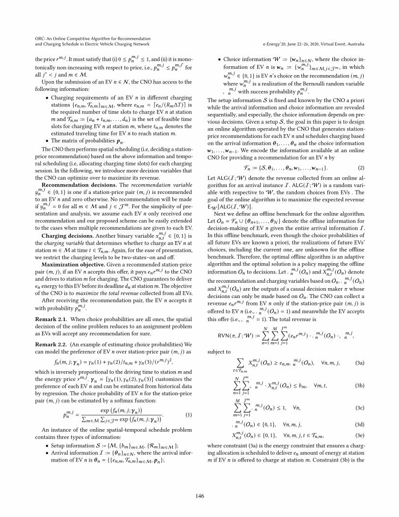
6.1 Simulation parameters6.1.1 Real-world transportation network. We focus on a sim-
plified transportation network in Hong Kong. The city is divided
into 18 districts, which are connected by 32 main roads as shown in
Figure 1. The traveling time through each main road is estimated
based on Google map data. We assume that there are four public
charging stations that can provide charging services for private
EVs. The setup information of the four stations is listed in Table 1.
6.1.2 Generating EV requests. Each arriving session 𝑛 ∈ N in
the experiments is a tuple of random variables (𝐴𝑛, 𝐸𝑛, 𝐷𝑛) ∈ R3
+where 𝐴𝑛 is the submission time; 𝐸𝑛 is the energy to be delivered
and 𝐷𝑛 is its deadline.
The arrival times {𝐴𝑛 : 𝑛 ∈ N} are generated according to a non-homogeneous Poisson process, with arrival rate being the product
of the time-varying demand function depicted in Figure 2(a) and
the average total number of EV arrivals, which is 600 multiplied
by a load factor 𝜌 > 0. We generate EV requests with varying
𝜌 ∈ {0.6, . . . , 1.6} to investigate the impact of the total number
of requests on the performance of online algorithms. The demand
function describes the percentage of the hourly refueling demand of
gasoline stations within one week [14]. Therefore, the total number
of arriving sessions 𝑁 is a Poisson random variable with mean 600𝜌 .
The total number of arriving sessions are further divided into 18
districts proportionally according to its corresponding normalized
population density, which is visualized in Figure 2(b).
After assigning an arriving session 𝑛 ∈ N to the districts, we
estimate the driving times 𝑡𝑛,𝑚 to the four stations based on the
shortest paths in the transportation network shown in Figure 1.
The energy demand 𝐸𝑛 is a uniform random variable defined on
[12, 24] (kWh). We set the deadline as 𝐷𝑛 = 𝐴𝑛 + 𝑡𝑛,𝑚 + 𝑀𝑛 + 𝑈
where 𝐴𝑛 + 𝑡𝑛,𝑚 is when the EV (if it accepts the recommendation)
3
9
8
1 2
6
5 4
14
13
11
15
17
16
New Territories
Kowloon
HK Island
7
10
18
Charging Station
Station A
Station B
Station C
Station D
12
Figure 1: Simplified transportation network of Hong Kong.
Table 1: Setup of Charging Stations
Station ID Location No. of Chargers Prices (cents/kWh)
A District 7 10 {40, 55, 75}B District 10 10 {50, 70, 90}C District 12 20 {50, 70, 90}D District 18 20 {60, 90, 110}
Mon Tue Wed Thu Fri Sat Sun0
0.002
0.004
0.006
0.008
0.01
0.012
0.014
Per
centa
ge
of
hourl
y d
eman
d
(a) Demand for EV charging
0 5 10 150
0.05
0.1
0.15
District ID
Norm
aliz
ed P
opula
tion D
ensi
ty(b) Population density of 18 districts
Figure 2: Time-varying demand for EV charging and geo-graphically distributed population density.
arrives at the charging station 𝑚; 𝑀𝑛 := 𝐸𝑛/𝑅𝑛 is its minimum
charging time and𝑈 is a random variable uniformly distributed in
[0, 2] (hours). The charging rate is set as 𝑅𝑛 = 6,∀𝑛 ∈ N (kW).
6.1.3 Estimating choice probabilities. Weuse the choicemodel
described in Remark 2.2 to estimate the choice probability. Partic-
ularly, we sample the three preference parameters 𝜸𝑛 uniformly
from [0, 1], [20, 30], and [12000, 14000] for each EV 𝑛.
6.2 BenchmarksWe compare our ORC( ˜𝜙) with the following three benchmark on-
line algorithms. These benchmarks use the same scheduling al-
gorithm for EV charging by greedily assigning the energy to the
time slots with lowest utilization of chargers. They, however, dif-
fer in the sense that they adopt different rules for selecting the
recommendations.
• Myopic. This algorithm recommends (𝑚, 𝑗) that maximizes
the expected revenue of the current EV by solving the prob-
lem (7) without considering future EV arrivals and the im-
balance of the charging demand over different stations.
152

e-Energy’20, June 22–26, 2020, Virtual Event, Australia B. Sun, T. Li, S.H. Low, and D.H.K. Tsang
0.6 0.8 1 1.2 1.4 1.60.4
0.5
0.6
0.7
0.8
0.9
1
1.1
1.2
1.3
Load factor
Em
pir
ical
Rat
ios
ORC
Myopic
Heuristic−Conservative
Heuristic−Greedy
Figure 3: Comparison of empirical ratios achieved by differ-ent online algorithms. Results are averaged over 100 inde-pendent simulations.
• Heuristic-Greedy. This algorithm recommends the nearest
charging station that is feasible to schedule the charging
with the lowest price.
• Heuristic-Conservative. In contrast toHeuristic-Greedy, thisalgorithm offers the nearest station at the highest price.
We compute the total revenue collected by each online algorithm
listed above. In each independent simulation, the arriving sessions
{(𝐴𝑛, 𝐸𝑛, 𝐷𝑛) : 𝑛 ∈ N} are generated randomly as described in
Section 6.1.2 and the EV accepts the recommendation according to
the choice probabilities in (1). The final results are averaged over
100 independent simulations.
Let 𝑅ALG denote the total revenue of an online algorithm ALGin each simulation and let 𝑅OPT denote the optimal value of the
upper bound problem (6), which is linear and can be solved by
the interior-point algorithm. We compare ORC( ˜𝜙) with the three
benchmark algorithms based on their empirical ratio, defined as
Empirical Ratio of ALG = 𝑅ALG/𝑅OPT . (25)
Since it is computationally difficult to obtain the optimal offline
decision 𝜋∗ in (4), we choose the optimal benchmark of the em-
pirical ratio as the upper bound of the expected optimal revenue.
Therefore, the average of the empirical ratio is a lower bound of
the competitive ratio (5). Moreover, the empirical ratio is defined
for each realization of EVs’ random choices, and hence, the total
collected revenue sometimes can be greater than the upper bound
of the expected revenue. Thus, the empirical ratio may be larger
than one for certain realizations. But the average empirical ratio cor-
responding to each arrival instance (i.e., average of 100 simulations)
is guaranteed to be smaller than one.
6.3 Performance evaluationThe numerical results are shown in Figures 3 and 4, with load
factors selected from {0.6, . . . , 1.6}.Figure 3 compares the empirical ratios that are achieved by our
proposed ORC and other three benchmark online algorithms. For
each arrival instance, the empirical ratios of ORC generally out-
perform those of all benchmark algorithms and ORC achieves the
largest average empirical ratio for all arrival instances. The figure
also highlights that the average empirical ratio forORC is very close
to 1, which is much larger than the theoretical competitive ratio
0.6 0.8 1 1.2 1.4 1.60.2
0.3
0.4
0.5
0.6
0.7
0.8
0.9
1
Load factor
Aver
age
Acc
epta
nce
Rat
ios
ORC
Myopic
Heuristic−Conservative
Heuristic−Greedy
Figure 4: Comparison of the average acceptance ratiosachieved by different online algorithms. Results are aver-aged over 100 independent simulations.
0.254 for this simulation setup. This theoretical value is calculated
by solving Equation (28) to obtain {ℓ̂𝑚,1}∀𝑚∈M based on bisection
search, and then substituting it to the expression of 𝛼˜𝜙in Theorem
4.4. The main reason is that the competitive ratio is derived for the
worse-case scenario for all possible arriving instances. Moreover,
with the increase of the load factor 𝜌 , the performance gap between
ORC and Myopic increases. This is because balancing the demand
over stations and reserving capacity for future arrivals become
more important in high-demand cases, which is also the reason
for that the greedy and conservative heuristics perform worse and
better, respectively as 𝜌 becomes larger.
Figure 4 displays the average acceptance ratios, i.e., the ratio of
the number of served charging sessions and that of the total charg-
ing sessions. Myopic and Heuristic-Greedy serve more charging
sessions in all cases since both algorithms recommend available
charging stations and allocate available chargers in an aggressive
manner without reserving some chargers for future EV arrivals,
which may accept higher prices. In comparison, our proposed ORCachieves a medium average acceptance ratio to trade off the ag-
gressiveness and conservativeness when allocating the resources
without future information. In this way, ORC achieves a much
better expected total revenue as shown in Figure 3.
7 CONCLUSIONSIn this paper we introduce an online algorithm, ORC, that canjointly decide recommendation and charging schedules for sequen-
tial EV arrivals in a network of charging stations. Sufficient con-
ditions for ensuring that ORC has a constant competitive ratio
are provided. Based on the conditions, we design an explicit value
function for ORC and its competitive ratio is also given. Numerical
experiments validate the effectiveness of ORC by showing that it
outperforms other benchmark online algorithms.
ACKNOWLEDGMENTSBo Sun and Danny H.K. Tsang’s research is supported in part by
the Hong Kong Research Grant Council (RGC) General Research
Fund (Project 16207318 and 16202619). Tongxin Li and Steven H.
Low’s research is supported by National Science Foundation (NSF)
through grants (CPS ECCS 1932611 and CPS ECCS 1739355).
153

ORC: An Online Competitive Algorithm for Recommendationand Charging Schedule in Electric Vehicle Charging Network e-Energy’20, June 22–26, 2020, Virtual Event, Australia
REFERENCES[1] B. Alinia, M. H. Hajiesmaili, and N. Crespi. 2019. Online EV Charging Scheduling
With On-Arrival Commitment. IEEE Transactions on Intelligent TransportationSystems 20, 12 (Dec 2019), 4524–4537.
[2] B. Alinia, M. H. Hajiesmaili, Z. J. Lee, N. Crespi, and E. Mallada. 2020. Online
EV Scheduling Algorithms for Adaptive Charging Networks with Global Peak
Constraints. IEEE Transactions on Sustainable Computing (2020), 1–1.
[3] B. Alinia, M. S. Talebi, M. H. Hajiesmaili, A. Yekkehkhany, and N. Crespi.
2018. Competitive Online Scheduling Algorithms with Applications in Deadline-
Constrained EV Charging. In 2018 IEEE/ACM 26th International Symposium onQuality of Service (IWQoS). 1–10.
[4] M. Alizadeh, H. Wai, M. Chowdhury, A. Goldsmith, A. Scaglione, and T. Javidi.
2017. Optimal Pricing to Manage Electric Vehicles in Coupled Power and Trans-
portation Networks. IEEE Transactions on Control of Network Systems 4, 4 (Dec2017), 863–875.
[5] Niv Buchbinder, Joseph Seffi Naor, et al. 2009. The design of competitive online
algorithms via a primal–dual approach. Foundations and Trends® in TheoreticalComputer Science 3, 2–3 (2009), 93–263.
[6] K. Clement-Nyns, E. Haesen, and J. Driesen. 2010. The Impact of Charging Plug-
In Hybrid Electric Vehicles on a Residential Distribution Grid. IEEE Transactionson Power Systems 25, 1 (Feb 2010), 371–380.
[7] L. Gan, U. Topcu, and S. H. Low. 2013. Optimal decentralized protocol for electric
vehicle charging. IEEE Transactions on Power Systems 28, 2 (May 2013), 940–951.
[8] Negin Golrezaei, Hamid Nazerzadeh, and Paat Rusmevichientong. 2014. Real-
Time Optimization of Personalized Assortments. Management Science 60, 6 (2014),1532–1551.
[9] L. Guo, K. F. Erliksson, and S. H. Low. 2017. Optimal online adaptive electric
vehicle charging. In 2017 IEEE Power Energy Society General Meeting. 1–5.[10] T. Guo, P. You, and Z. Yang. 2017. Recommendation of geographic distributed
charging stations for electric vehicles: A game theoretical approach. In 2017 IEEEPower Energy Society General Meeting. 1–5.
[11] Zhiyi Huang and Anthony Kim. 2019. Welfare maximization with production
costs: A primal dual approach. Games and Economic Behavior 118 (2019), 648 –667.
[12] Will Ma and David Simchi-Levi. 2019. Algorithms for online matching, assort-
ment, and pricing with tight weight-dependent competitive ratios. arXiv preprintarXiv:1905.04770 (2019).
[13] A. Moradipari and M. Alizadeh. 2020. Pricing and Routing Mechanisms for
Differentiated Services in an Electric Vehicle Public Charging Station Network.
IEEE Transactions on Smart Grid 11, 2 (2020), 1489–1499.
[14] Sarah G. Nurre, Russell Bent, Feng Pan, and Thomas C. Sharkey. 2014. Managing
operations of plug-in hybrid electric vehicle (PHEV) exchange stations for use
with a smart grid. Energy Policy 67 (2014), 364 – 377.
[15] B. Sun, X. Tan, and D. H. K. Tsang. 2019. Eliciting Multi-Dimensional Flexibilities
From Electric Vehicles: A Mechanism Design Approach. IEEE Transactions onPower Systems 34, 5 (Sep. 2019), 4038–4047.
[16] Kalyan Talluri and Garrett Van Ryzin. 1998. An Analysis of Bid-Price Controls
for Network Revenue Management. Manage. Sci. 44, 11 (Nov. 1998), 1577–1593.[17] X. Tan, A. Leon-Garcia, Bo Sun, and D. H. K. Tsang. 2019. A Novel Online
Mechanism for Demand-Side Flexibility Management under Arbitrary Arrivals.
In Proceedings of the Tenth ACM International Conference on Future Energy Systems(Phoenix, AZ, USA) (e-Energy ’19). Association for Computing Machinery, New
York, NY, USA, 391–392.
[18] X. Tan, A. Leon-Garcia, Y. Wu, and D. H. K. Tsang. 2020. Online Combinatorial
Auctions for Resource Allocation with Supply Costs and Capacity Limits. IEEEJournal on Selected Areas in Communications (2020), 1–1.
[19] W. Tang, S. Bi, and Y. J. Zhang. 2014. Online coordinated charging decision
algorithm for electric vehicles without future information. IEEE Transactions onSmart Grid 5, 6 (Nov 2014), 2810–2824.
[20] Z. Tian, T. Jung, Y. Wang, F. Zhang, L. Tu, C. Xu, C. Tian, and X. Li. 2016. Real-
Time Charging Station Recommendation System for Electric-Vehicle Taxis. IEEETransactions on Intelligent Transportation Systems 17, 11 (Nov 2016), 3098–3109.
[21] P. You, Z. Yang, Y. Zhang, S. H. Low, and Y. Sun. 2016. Optimal Charging Schedule
for a Battery Switching Station Serving Electric Buses. IEEE Transactions onPower Systems 31, 5 (Sep. 2016), 3473–3483.
[22] Xiaoxi Zhang, Zhiyi Huang, Chuan Wu, Zongpeng Li, and Francis C. M. Lau.
2017. Online Auctions in IaaS Clouds: Welfare and Profit Maximization With
Server Costs. IEEE/ACM Trans. Netw. 25, 2 (April 2017), 1034–1047.[23] S. Zhao, X. Lin, andM. Chen. 2015. Peak-minimizing online EV charging: Price-of-
uncertainty and algorithm robustification. In 2015 IEEE Conference on ComputerCommunications (INFOCOM). 2335–2343.
[24] Zizhan Zheng and Ness Shroff. 2014. Online Welfare Maximization for Electric
Vehicle Charging with Electricity Cost. In Proceedings of the 5th InternationalConference on Future Energy Systems (Cambridge, United Kingdom) (e-Energy’14). Association for Computing Machinery, New York, NY, USA, 253–263.
[25] M. Zhu, X. Liu, and X.Wang. 2018. Joint Transportation and Charging Scheduling
in Public Vehicle Systems—A Game Theoretic Approach. IEEE Transactions on
Intelligent Transportation Systems 19, 8 (Aug 2018), 2407–2419.
A PROOF OF LEMMA 2.3Let {𝑌𝑚,𝑗
𝑛 (O𝑛), 𝑋𝑚,𝑗𝑛,𝑡 (O𝑛)} denote the decisions made by the op-
timal decision rule 𝜋∗ for EV 𝑛 with the offline information O𝑛 .
𝑌𝑚,𝑗𝑛 (O𝑛) and 𝑋
𝑚,𝑗𝑛,𝑡 (O𝑛) only depend on the realizations of EVs’
choices, i.e.,𝒘1, . . . ,𝒘𝑛−1. Therefore, 𝑌𝑚,𝑗𝑛 (O𝑛) and 𝑋𝑚,𝑗
𝑛,𝑡 (O𝑛) areboth independent of𝑊
𝑚,𝑗𝑛 . Let 𝑦
𝑚,𝑗𝑛 = E[𝑌𝑚,𝑗
𝑛 (O𝑛)] and 𝑥𝑚,𝑗𝑛𝑡 =
E[𝑋𝑚𝑛,𝑡 (O𝑛)], where the expectation is taken with respective to the
previous 𝑛 − 1 EVs’ random choices. The optimal expected revenue
can be denoted by
EW [OPT(I;W)] =𝑁∑𝑛=1
𝑀∑𝑚=1
𝐽∑𝑗=1
(𝑒𝑛𝑟𝑚,𝑗 ) · EW [𝑊𝑚,𝑗𝑛 · 𝑌𝑚,𝑗
𝑛 (O𝑛)],
=
𝑁∑𝑛=1
𝑀∑𝑚=1
𝐽∑𝑗=1
(𝑒𝑛𝑟𝑚,𝑗 ) · 𝑝𝑚,𝑗𝑛 · 𝑦𝑚,𝑗
𝑛 ,
which is the objective of the problem (6) when 𝑦𝑚,𝑗𝑛 = 𝑦
𝑚,𝑗𝑛 . If
we can show {𝑦𝑚,𝑗𝑛 }𝑛,𝑚,𝑗 and {𝑥𝑚,𝑗
𝑛,𝑡 }𝑛,𝑡,𝑚,𝑗 are a feasible solution
to the problem (6), it follows EW [OPT(I;W)] ≤ OPT(I). Sinceconstraints (3a)-(3e) are respected by the optimal decision rules
for any realizations ofW, we can take expectation on both sides
of these constraints and this leads to the constraints (6b)-(6f) with
{𝑦𝑚,𝑗𝑛 }𝑛,𝑚,𝑗 and {𝑥𝑚,𝑗
𝑛,𝑡 }𝑛,𝑡,𝑚,𝑗 being substituted. Note that we use
the independence of 𝑋𝑚,𝑗𝑛,𝑡 (O𝑛) and𝑊𝑚,𝑗
𝑛 when taking expectation
for (3b). Thus, {𝑦𝑚,𝑗𝑛 }𝑛,𝑚,𝑗 and {𝑥𝑚,𝑗
𝑛,𝑡 }𝑛,𝑡,𝑚,𝑗 are a feasible solution
to the problem (6) and hence EW [OPT(I;W)] is an upper bound
of OPT(I).
B PROOF OF LEMMA 5.2Conditional on F𝑛 or equivalently the random choices of the previ-
ous 𝑛 − 1 EVs {𝒘1, . . . ,𝒘𝑛−1}, 𝑌𝑚,𝑗𝑛 , 𝑋
𝑚,𝑗𝑛,𝑡 and 𝑉𝑚
𝑛−1,𝑡are all deter-
ministic values. We then have the conditional expectation
E[𝐻𝑛 |F𝑛] = E
𝑀∑
𝑚=1
𝐽𝑚∑𝑗=1
𝑌𝑚,𝑗𝑛 𝑊
𝑚,𝑗𝑛 (𝑟𝑚,𝑗 − Λ
𝑚,𝑗𝑛 )𝑒𝑛 |F𝑛
=
𝑀∑𝑚=1
𝐽𝑚∑𝑗=1
𝑌𝑚,𝑗𝑛 𝑝
𝑚,𝑗𝑛 (𝑟𝑚,𝑗 − Λ
𝑚,𝑗𝑛 )𝑒𝑛, (26)
(𝑖)= max
{max𝑚∈M, 𝑗 ∈J𝑚 𝑝
𝑚,𝑗𝑛 (𝑟𝑚,𝑗 − Λ
𝑚,𝑗𝑛 )𝑒𝑛, 0
},
≥ 𝑝𝑚,𝑗𝑛 (𝑟𝑚,𝑗 − Λ
𝑚,𝑗𝑛 )𝑒𝑛,∀𝑚 ∈ M, 𝑗 ∈ J𝑚 .
Equality (𝑖) holds since 𝑌𝑚,𝑗𝑛 is determined based on Equations (10)
and (11) to choose themaximumnon-negative 𝑝𝑚,𝑗𝑛 (𝑟𝑚,𝑗−Λ𝑚,𝑗
𝑛 ). Bytaking expectation on both sides of above equation with respective
to F𝑛 and applying tower property, we show that [̄𝑛 and¯_𝑚,𝑗𝑛 satisfy
the constraint (18b), namely,
[̄𝑛 = E[𝐻𝑛] = EF𝑛 [E[𝐻𝑛 |F𝑛]]
≥ EF𝑛 [𝑝𝑚,𝑗𝑛 (𝑟𝑚,𝑗 − Λ
𝑚,𝑗𝑛 )𝑒𝑛]
= 𝑝𝑚,𝑗𝑛 (𝑟𝑚,𝑗 − ¯_
𝑚,𝑗𝑛 )𝑒𝑛,∀𝑚 ∈ M, 𝑗 ∈ J𝑚 .
154

e-Energy’20, June 22–26, 2020, Virtual Event, Australia B. Sun, T. Li, S.H. Low, and D.H.K. Tsang
Next, by taking conditional expectation on 𝐵𝑚,𝑗𝑛,𝑡 , we have
E[𝐵𝑚,𝑗𝑛,𝑡 |F𝑛] = 𝑋
𝑚,𝑗𝑛,𝑡 𝑝
𝑚,𝑗𝑛 [Λ𝑚,𝑗
𝑛 − 𝜙𝑚 (𝑉𝑚𝑛−1,𝑡/𝑏𝑚)], (27)
(𝑖𝑖)≥ 𝑝
𝑚,𝑗𝑛 [Λ𝑚,𝑗
𝑛 − 𝜙𝑚 (𝑉𝑚𝑛−1,𝑡 /𝑏𝑚)],
≥ 𝑝𝑚,𝑗𝑛 [Λ𝑚,𝑗
𝑛 − 𝜙𝑚 (𝑉𝑚𝑁,𝑡/𝑏𝑚)] .
When 𝑋𝑚,𝑗𝑛,𝑡 = 1, inequality (ii) holds naturally. When 𝑋
𝑚,𝑗𝑛,𝑡 = 0,
there exist two cases. If the station-price (𝑚, 𝑗) is not offered, i.e.,𝑌𝑚,𝑗𝑛 = 0, Λ
𝑚,𝑗𝑛 = 0 by definition in (20) and inequality (ii) holds. If
(𝑚, 𝑗) is offered while the EV 𝑛 is not scheduled to charge at time
𝑡 , we have Λ𝑚,𝑗𝑛 − 𝜙𝑚 (𝑉𝑚
𝑛−1,𝑡/𝑏𝑚) ≤ 0, i.e., the cost of activating
one more charger at time 𝑡 is no less than the marginal cost of the
charging session 𝑛 at station𝑚. Thus, inequality (ii) still holds in
this case. Since 𝑉𝑚𝑛−1,𝑡
≤ 𝑉𝑚𝑁,𝑡
and the value function 𝜙𝑚 is non-
decreasing, the last inequality holds. Finally, we take expectation
with respective to F𝑛 on both sides of above inequality and we
show ¯̀𝑚𝑡 ,
¯_𝑚,𝑗𝑛 , and
¯𝛽𝑚,𝑗𝑛,𝑡 satisfy the constraint (18c).
¯𝛽𝑚,𝑗𝑛,𝑡 = E[𝐵𝑚,𝑗
𝑛,𝑡 ] = EF𝑛 [E[𝐵𝑚,𝑗𝑛,𝑡 |F𝑛]]
≥ EF𝑛 [𝑝𝑚,𝑗𝑛 [Λ𝑚,𝑗
𝑛 − 𝜙𝑚 (𝑉𝑚𝑁,𝑡/𝑏𝑚)]],
= 𝑝𝑚,𝑗𝑛 ( ¯_
𝑚,𝑗𝑛 − ¯̀
𝑚𝑡 ),∀𝑛 ∈ N ,𝑚 ∈ M, 𝑗 ∈ J𝑚, 𝑡 ∈ T𝑛,𝑚 .
C PROOF OF LEMMA 5.4Define the length of the 𝑗-th segment as 𝜎𝑚,𝑗 = ℓ𝑚,𝑗 − ℓ𝑚,𝑗−1,∀𝑗 ∈J𝑚
. Based on Equation (23), 𝜎𝑚,𝑗can be represented as a function
of 𝜎𝑚,1, i.e.,
𝜎𝑚,𝑗 = − ln
[𝑟𝑚,𝑗−1
𝑟𝑚,𝑗+
(1 − 𝑟𝑚,𝑗−1
𝑟𝑚,𝑗
)𝑒−𝜎
𝑚,1
], 𝑗 = 2, . . . , 𝐽𝑚 .
Since
∑𝑗 ∈J𝑚 𝜎𝑚,𝑗 = 1, we have
𝑒−𝜎𝑚,1
∏𝐽𝑚
𝑗=2
[𝑟𝑚,𝑗−1
𝑟𝑚,𝑗+
(1 − 𝑟𝑚,𝑗−1
𝑟𝑚,𝑗
)𝑒−𝜎
𝑚,1
]= 𝑒−1 . (28)
Define 𝑔(𝜎𝑚,1) as the left hand side of the above equation. 𝑔(𝜎𝑚,1)is a non-increasing function in [0, 1] with 𝑔(0) = 1 and
𝑔(1) = 𝑒−1
∏𝐽𝑚
𝑗=2
[𝑟𝑚,𝑗−1
𝑟𝑚,𝑗(1 − 𝑒−1) + 𝑒−1
]< 𝑒−1 .
Thus, there must exist a solution to 𝑔(𝜎𝑚,1) = 𝑒−1and hence there
exists segments points {ℓ̂𝑚,𝑗 }𝑗 ∈J𝑚 that satisfy Equation (23). Since
𝑔(𝜎𝑚,1) is monotonic in [0, 1], bisection search can be used to find
𝜎𝑚,1. We can then compute all segment points {ℓ̂𝑚,𝑗 }𝑗 ∈J𝑚 .
D PROOF OF LEMMA 5.5We check the inequality in the following three cases.
Case (i): when 𝑞 = ⌈ℓ̂𝑚,𝑗𝑏𝑚⌉/𝑏𝑚 − 1/𝑏𝑚 , we have[˜𝜙𝑚 (𝑞 + 1/𝑏𝑚) − ˜𝜙𝑚 (𝑞)
]𝑏𝑚 + 𝑟𝑚,𝑗 − ˜𝜙𝑚 (𝑞)
(𝑖)=
[𝜙𝑚 (ℓ̂𝑚,𝑗 ) − 𝜙𝑚 (𝑞)
]𝑏𝑚 + 𝜙𝑚 (ℓ̂𝑚,𝑗 ) − 𝜙𝑚 (𝑞),
(𝑖𝑖)=
𝑟𝑚,𝑗 − 𝑟𝑚,𝑗−1
𝑒 ℓ̂𝑚,𝑗 − 𝑒 ℓ̂
𝑚,𝑗−1
[𝑒 ℓ̂
𝑚,𝑗
− 𝑒𝑞](𝑏𝑚 + 1),
= 𝑟𝑚,𝑗 · 1 − 𝑟𝑚,𝑗−1/𝑟𝑚,𝑗
1 − 𝑒−(ℓ̂𝑚,𝑗−ℓ̂𝑚,𝑗−1)
[1 − 𝑒𝑞−ℓ̂
𝑚,𝑗](𝑏𝑚 + 1),
(𝑖𝑖𝑖)=
𝑟𝑚,𝑗
𝛼
[1 − 𝑒𝑞−ℓ̂
𝑚,𝑗](𝑏𝑚 + 1) ≤ 𝑟𝑚,𝑗
𝛼(𝑏𝑚 + 1) (1 − 𝑒−1/𝑏𝑚 ),
where equalities (i) and (ii) are obtained by substituting˜𝜙𝑚 and 𝜙𝑚
in Equations (14) and (15), and equality (iii) is from Equation (23).
Case (ii): when ⌈ℓ̂𝑚,𝑗−1𝑏𝑚⌉/𝑏𝑚 < 𝑞 < ⌈ℓ̂𝑚,𝑗𝑏𝑚⌉/𝑏𝑚 − 1/𝑏𝑚 .[˜𝜙𝑚 (𝑞 + 1/𝑏𝑚) − ˜𝜙𝑚 (𝑞)
]𝑏𝑚 + 𝑟𝑚,𝑗 − ˜𝜙𝑚 (𝑞)
= [𝜙𝑚 (𝑞 + 1/𝑏𝑚) − 𝜙𝑚 (𝑞)] 𝑏𝑚 + 𝜙𝑚 (ℓ̂𝑚,𝑗 ) − 𝜙𝑚 (𝑞),
=𝑟𝑚,𝑗 − 𝑟𝑚,𝑗−1
𝑒 ℓ̂𝑚,𝑗 − 𝑒 ℓ̂
𝑚,𝑗−1
[(𝑏𝑚 − (𝑏𝑚 + 1)𝑒−1/𝑏𝑚 )𝑒𝑞+1/𝑏𝑚 + 𝑒 ℓ̂
𝑚,𝑗],
(𝑖𝑣)≤ 𝑟𝑚,𝑗 − 𝑟𝑚,𝑗−1
𝑒 ℓ̂𝑚,𝑗 − 𝑒 ℓ̂
𝑚,𝑗−1
[(𝑏𝑚 − (𝑏𝑚 + 1)𝑒−1/𝑏𝑚 )𝑒 ℓ̂
𝑚,𝑗
+ 𝑒 ℓ̂𝑚,𝑗
],
=𝑟𝑚,𝑗
𝛼(𝑏𝑚 + 1) (1 − 𝑒−1/𝑏𝑚 ),
where inequality (iv) holds since 𝑏𝑚 − (𝑏𝑚 + 1)𝑒−1/𝑏𝑚 ≥ 0 for
𝑏𝑚 = 1, 2, . . . , and 𝑞 + 1/𝑏𝑚 ≤ ℓ̂𝑚,𝑗.
Case (iii): when 𝑞 = ⌈ℓ̂𝑚,𝑗−1𝑏𝑚⌉/𝑏𝑚 .[˜𝜙𝑚 (𝑞 + 1/𝑏𝑚) − ˜𝜙𝑚 (𝑞)
]𝑏𝑚 + 𝑟𝑚,𝑗 − ˜𝜙𝑚 (𝑞)
=[𝜙𝑚 (𝑞 + 1/𝑏𝑚) − 𝜙𝑚 (ℓ̂𝑚,𝑗−1)
]𝑏𝑚 + 𝜙𝑚 (ℓ̂𝑚,𝑗 ) − 𝜙𝑚 (ℓ̂𝑚,𝑗−1),
=𝑟𝑚,𝑗 − 𝑟𝑚,𝑗−1
𝑒 ℓ̂𝑚,𝑗 − 𝑒 ℓ̂
𝑚,𝑗−1
[(𝑏𝑚 − (𝑏𝑚 + 1)𝑒 ℓ̂
𝑚,𝑗−1−𝑞−1/𝑏𝑚 )𝑒𝑞+1/𝑏𝑚 + 𝑒 ℓ̂𝑚,𝑗
],
(𝑣)≤ 𝑟𝑚,𝑗 − 𝑟𝑚,𝑗−1
𝑒 ℓ̂𝑚,𝑗 − 𝑒 ℓ̂
𝑚,𝑗−1
[(𝑏𝑚 − (𝑏𝑚 + 1)𝑒 ℓ̂
𝑚,𝑗−1−𝑞−1/𝑏𝑚 )𝑒 ℓ̂𝑚,𝑗
+ 𝑒 ℓ̂𝑚,𝑗
],
≤ 𝑟𝑚,𝑗
𝛼(𝑏𝑚 + 1) (1 − 𝑒−2/𝑏𝑚 ).
Note that −2/𝑏𝑚 ≤ ℓ̂𝑚,𝑗−1 −𝑞 − 1/𝑏𝑚 ≤ −1/𝑏𝑚 . Thus, 𝑏𝑚 − (𝑏𝑚 +1)𝑒 ℓ̂𝑚,𝑗−1−𝑞−1/𝑏𝑚 ≥ 𝑏𝑚 − (𝑏𝑚 + 1)𝑒−1/𝑏𝑚 ≥ 0 and inequality (v)
holds. Combining the three cases, we have the inequality (24).
155
Recommended