Optofluidic Characterization of Porous Materials
Escuela de Materiales porosos Nanoestructurados
Raúl UrteagaSanta Fe - Octubre 2014
Congreso Internacional de Metalurgia y Materiales14 SAM- CONAMET
XIII Simposio Materia

Optofluídica
Caracterización óptofluídica de materiales:
_ Longitud de onda incidente mucho mayor que el tamaño de las estructuras:
Índice de refracción efectivo
_ Interferencia coherente de haces:
Capas delgadas
_ Imbibición capilar de líquidos en matriz porosa:
Fluidodinámica
Integración de la óptica y la microfluídica para obtener información de ambas en simultaneo [1].
[1] Psaltis et al. “Developing optofluidic technology through the fusion of microfluidics and optics.” Nature 2006, 442, 381−386.

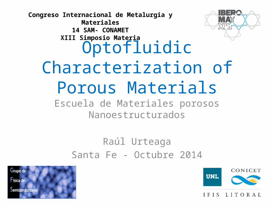
Thin film optical interference
For P- type polarization
F.L. Pedrotti, L.S. Pedrotti “Introduction to optics” 2nd Ed. Prentice-Hall inc. NJ (1993)
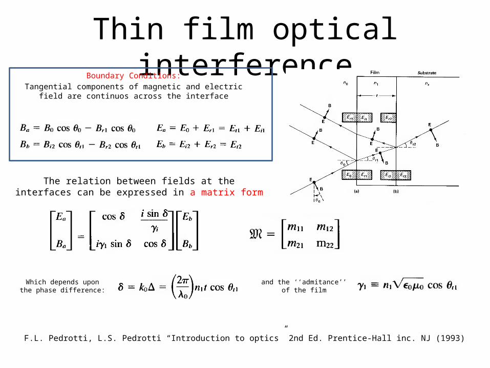
Thin film optical interference
F.L. Pedrotti, L.S. Pedrotti “Introduction to optics” 2nd Ed. Prentice-Hall inc. NJ (1993)
Boundary Conditions:Tangential components of magnetic and electric
field are continuos across the interface
The relation between fields at the interfaces can be expressed in a matrix form
Which depends upon the phase difference:
and the ‘‘admitance’’ of the film

Transfer Matrix formalismFor a multilayer
we have:
The reflection and transmission coefficients are
Can be calculated as
F.L. Pedrotti, L.S. Pedrotti “Introduction to optics” 2nd Ed. Prentice-Hall inc. NJ (1993)
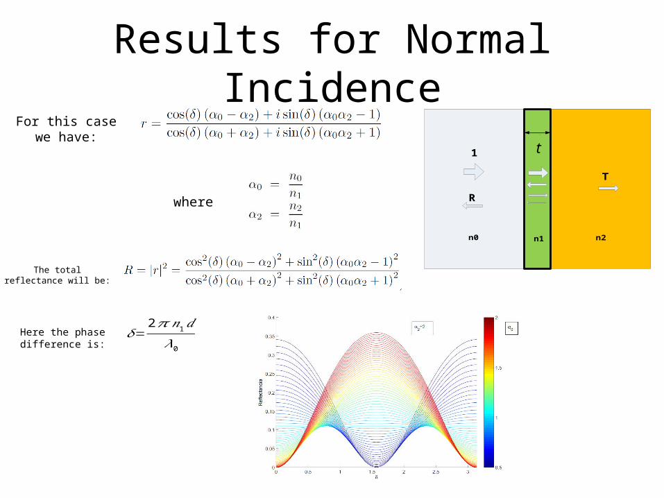
Results for Normal IncidenceFor this case we
have:
where
The total reflectance will be:
n0 n1 n2
1
T
R
d
t
𝛿=2𝜋 𝑛1𝑑𝜆0
Here the phase difference is:

Results for Normal Incidence
Important to note:(If δ is real )
n0 n1 n2
1
T
R
d
t
𝛿=2𝜋 𝑛1𝑑𝜆0
=> Periodic!
𝑛1𝑑=𝜆02
𝑛1𝑑=𝜆04

Results for Normal IncidenceIf reflectance is periodic, then the Fourier transform
in K space is discrete, and have peaks at 2nd
2𝑛1𝑑
If there is absortion (refractive index complex)

Optical Properties of Mixtures
To find these variables Maxwell's equations must be solved for electrostatic :
How to obtain the effective dielectric constant?
Geometry must be known and generally requires an expensive calculation

Effective Medium Theories
• Maxwell-Garnet
[2] O. Stenzel, The Physics of Thin Film Optical Spectra Springer Series in Surface Sciences Volume 44 (2005)
Cavidad [2] paralelo al eje perpendicular
Esfera ⅓ ⅓
Cilindro 0 ½
Placa 1 0
Elipsoide de ejes ,
𝜀 𝑗𝜀𝑙

Effective Medium Theories• Lorentz- Lorenz [2]
[2] O. Stenzel, The Physics of Thin Film Optical Spectra Springer Series in Surface Sciences Volume 44 (2005)[3] L.D. Landau, E.M. Lifshitz, Electrodynamics of Continuous Media, 2nd. Edition (vol. 8), Elsevier, Burlington, 1984.
• Bruggeman [2]
• Looyenga-Landau-Lifshithz [3]
𝜀 𝑗
𝜀 𝑗
𝜀𝑙=1
𝜀𝑙=𝜀
𝜀 𝑗𝜀𝑙 𝜀 𝑗

Effective Medium Theories
LimitsCavidad [2]
paralell PerpendicularEsfer ⅓ ⅓
Cylinder 0 ½
Plate 1 0

Effective Medium Theories
Refractive index of silicon and alumina [4].Alumina is transparent!
[4]
200 300 400 500 600 700 800 900 1000 1100 12000
1
2
3
4
5
6
7
[nm]
Silicon nreal
Silicon nimag
Alumina
𝑛=√𝜀

Effective Medium Theories
Example case I: Porous Silicon + Air
@ L=1/3
0 0.1 0.2 0.3 0.4 0.5 0.6 0.7 0.8 0.9 11
1.5
2
2.5
3
3.5
4
Porosity
Eff
ectiv
e re
frac
tive
inde
x
Maxwell-Garnet
Bruggeman
Looyenga

Effective Medium Theories
Example case II: Porous Alumina + Isopropyl Alcohol
0 0.1 0.2 0.3 0.4 0.5 0.6 0.7 0.8 0.9 11
1.1
1.2
1.3
1.4
1.5
1.6
1.7
1.8
Porosity
Eff
ectiv
e re
frac
tive
inde
x
Depolarization factor L: 0.5
Maxwell-Garnet dry alumina
Maxwell-Garnet wet aluminaBruggeman dry alumina
Burggeman wet alumina
@ L=1/2

Optical CharacterizationSpectroscopic reflectance of porous Silicon single layer

Optical CharacterizationSpectroscopic reflectance of porous Silicon Bragg reflector

Spectroscopic Liquid Infiltration method (SLIM)
1) Using FFT of the reflectance spectrum we can obtain an estimation of the optical width of the dry sample
𝑛𝑑𝑟𝑦𝑑
2) After infiltration we can measure the optical width of the wetted sample
𝑛𝑤𝑑
𝑛𝑤= 𝑓 (𝑃 ,𝑛𝐴𝑙 ,𝑛𝑙𝑖𝑞 )
Porous Alumina + Isopropyl Alcohol
3)The system can be solved to obtain P and d
M. J. Sailor Porous Silicon in Practice Preparation, Characterization and Applications Wiley-VCH Verlag & Co. (2012)
𝑛𝑑𝑟𝑦= 𝑓 (𝑃 ,𝑛𝐴𝑙 ,𝑛𝑎𝑖𝑟 )0 0.1 0.2 0.3 0.4 0.5 0.6 0.7 0.8 0.9 1
1
1.1
1.2
1.3
1.4
1.5
1.6
1.7
1.8
Porosity
Eff
ectiv
e re
frac
tive
inde
x
Depolarization factor L: 0.5
Maxwell-Garnet dry alumina
Maxwell-Garnet wet aluminaBruggeman dry alumina
Burggeman wet alumina

Fluid Mechanics at low ReI) Capillary filling of uniform closed channel
2r
Straight channel
Tortuous channel:L
L’
𝜏=𝐿𝐿 ′
In nondimensional form: were
L.N. Acquaroli, R. Urteaga, C.L.A. Berli, R.R. Koropecki, Langmuir 27, 2067 (2011)
Hagen-Poisseuille flow
Contact Angle
∆ 𝑃=𝜎 𝑐𝑜𝑠𝜃
𝑟
Laplace Pressure

Fluid Mechanics at low ReI) Uniform closed channel
Solving the differential equation:
The final position defines the value of
then
Lucas-Washburn Dynamics
𝑙2=12𝜎 𝑟𝜇𝑡
0
Tiempo
Posi
ción
Men
isco
tfill
L then
Edward W. Washburn “THE DYNAMICS OF CAPILLARY FLOW”The Physical Review Vol. XVII, 3, (1921)

Lateral view Top view
Optoflidic CharacterizationPorous Silicon

Dynamic SLIM
L.N. Acquaroli, R. Urteaga, C.L.A. Berli, R.R. Koropecki, Langmuir 27, 2067 (2011)
Normalized reflectance during the imbibition of a PS layer (15 μm thick, fabricated using a current density of 13 mA/cm2), with isopropyl alcohol at room temperature and the pressure of 1 atm.
Experimental setup What is measured (twice)

Relation between reflexion extremes and liquid infiltration
𝑒0=𝑛2(𝐿−𝑥 )+𝑛3𝑥
An extreme in reflectance will occur each time the optical path is a multiple of :
𝑛1𝑑=𝜆02
𝑛1𝑑=𝜆04
𝑒0=𝑚𝜆04
𝑒0=∫0
𝐿
𝑛𝑒𝑓𝑓 (𝑥 )𝑑𝑥
𝑑𝑒0𝑑𝑥
=𝑥 (𝑛3−𝑛2)
Between extremes in reflectance the interface moves
𝛥𝑥=𝜆
4 (𝑛3−𝑛2)

Results
L.N. Acquaroli, R. Urteaga, C.L.A. Berli, R.R. Koropecki, Langmuir 27, 2067 (2011)

Results
_Obtaining this values from the fit, it is posible to calulate the mean hidraulic radius and the tortuosity. _ The porosity and layer thicknes it is also obtained by SLIM
𝜏=𝐿𝐿 ′
2,6

Fluid Mechanics at low ReI) Variable section open channel
Direct problem:
R. Urteaga, L.N. Acquaroli, R.R. Koropecki, A. Santos, M. Alba, J. Pallares, L.F. Marsal, C.L.A. Berli, Langmuir 29, 2784 (2013)
𝑢( 𝑙 )=𝛼𝑟 (𝑙 )
−3
∫0
𝑙
𝑟 (𝑥 )− 4d 𝑥 𝛼=¿¿were
−𝜕𝑝𝜕 𝑥
=8𝜇𝑄𝜋𝑟 (𝑥 )
4
Poisseuille flow
𝛥𝑝=2𝛾 cos𝜃𝑟 (𝑥 )
Laplace Pressure

Fluid Mechanics at low ReI) Variable section open channel
Has multiple solutions!!
Inverse problem [5]:
as input
as input
𝑟 ( 𝑙 )=[𝑟 (𝐿 )𝑢(𝐿 )
13 + 13𝛼∫𝑙
𝐿
𝑢( 𝑙 )
43 dl ]𝑢 (𝑙 )
− 13
[5] E. Elizalde, R. Urteaga, R.R. Koropecki, C.L.A. Berli, Phys. Rev. Lett. 112, 134502 (2014)
𝑟 (𝑣 )=[𝑟❑ (𝑉 )
5 𝑄(𝑉 )5 + 5
𝜋 2𝛼∫𝑣
𝑉
𝑄 (𝑣 )6 dv ]
15𝑄 (𝑣 )
−1

Experimental setup
Optoflidic CharacterizationPorous Alumina
Top side Bottom side
E. Elizalde, R. Urteaga, R.R. Koropecki, C.L.A. Berli, Phys. Rev. Lett. 112, 134502 (2014)

Results
Optoflidic CharacterizationPorous Alumina
E. Elizalde, R. Urteaga, R.R. Koropecki, C.L.A. Berli, Phys. Rev. Lett. 112, 134502 (2014)
Radii at the ends coincide with SEM photographs

Thanks

Relation between reflexion extremes and liquid infiltration
𝑒0=𝑛2(𝐿−𝑥 )+𝑛3𝑥
An extreme in reflectance will occur each time the optical path is a multiple of :
𝑛1𝑑=𝜆02
𝑛1𝑑=𝜆04
𝑒0=𝑚𝜆04
𝑒0=∫0
𝐿
𝑛𝑒𝑓𝑓 (𝑥 )𝑑𝑥
𝑑𝑒0𝑑𝑥
=𝑥 (𝑛3(x )−𝑛2(𝑥 ))
Between extremes in reflectance the interface moves
𝛥𝑥=𝜆
4 (𝑛3 (𝑥)−𝑛2 (𝑥))=
𝜆4 (𝑛𝑤 (𝑥)−𝑛𝑑𝑟𝑦 (𝑥))

𝑛𝑤−𝑛𝑑𝑟𝑦= 𝑓 (𝑃 ) (𝑛¿¿ 𝑙𝑖𝑞𝑢𝑖𝑑−1)𝑃 ¿
The linear approximation
Porous Alumina + Isopropyl Alcohol
0 0.1 0.2 0.3 0.4 0.5 0.6 0.7 0.8 0.9 11
1.1
1.2
1.3
1.4
1.5
1.6
1.7
1.8
Porosity
Eff
ectiv
e re
frac
tive
inde
x
Depolarization factor L: 0.5
Maxwell-Garnet dry alumina
Maxwell-Garnet wet aluminaBruggeman dry alumina
Burggeman wet alumina
Relative difference from linear
0 0.2 0.4 0.6 0.8 1-0.05
-0.04
-0.03
-0.02
-0.01
0
Porosity
Rel
ativ
e di
fere
nce
Modelo de Bruggeman. Depolarization factor: 0.5
𝛥𝑥=𝜆
4 (𝑛3 (𝑥)−𝑛2 (𝑥))

Recommended