1
A Decision Rule to Minimize Daily Capital Charges
in Forecasting Value-at-Risk*
Michael McAleer
Department of Quantitative Economics Complutense University of Madrid
and Econometric Institute
Erasmus University Rotterdam
Juan-Angel Jimenez-Martin
Department of Quantitative Economics Complutense University of Madrid
Teodosio Pérez-Amaral
Department of Quantitative Economics Complutense University of Madrid
February 2009
* This paper was written while the first author was visiting the Econometric Institute, Erasmus School of Economics, Erasmus University Rotterdam, in autumn 2008. The first author wishes to thank the Australian Research Council for financial support, and the Erasmus School of Economics for their gracious hospitality and excellent working environment. We wanted to thank Jesus Ruiz for his help with graphs.
2
Abstract
Under the Basel II Accord, banks and other Authorized Deposit-taking Institutions
(ADIs) have to communicate their daily risk estimates to the monetary authorities at the
beginning of the trading day, using a variety of Value-at-Risk (VaR) models to measure
risk. Sometimes the risk estimates communicated using these models are too high,
thereby leading to large capital requirements and high capital costs. At other times, the
risk estimates are too low, leading to excessive violations, so that realised losses are
above the estimated risk. In this paper we propose a learning strategy that complements
existing methods for calculating VaR and lowers daily capital requirements, while
restricting the number of endogenous violations within the Basel II Accord penalty
limits. We suggest a decision rule that responds to violations in a discrete and
instantaneous manner, while adapting more slowly in periods of no violations. We
apply the proposed strategy to Standard & Poor’s 500 Index and show there can be
substantial savings in daily capital charges, while restricting the number of violations to
within the Basel II penalty limits.
Key words and phrases: Daily capital charges, endogenous violations, frequency of
violations, optimizing strategy, risk forecasts, value-at-risk.
JEL Classifications: G32, G11, G17, C53.
3
1. Introduction
The Value-at-Risk (VaR) concept has become a standard tool in the exploding area of
risk measurement and management. In brief, VaR is defined as an estimate of the
probability and size of the potential loss to be expected over a given period. This
concept has become especially important following the 1995 amendment to the Basel
Accord, whereby banks and other Authorized Deposit-taking Institutions (ADIs) were
permitted to use internal models to calculate their VaR thresholds (see Jorion (2000) for
a detailed discussion of VaR). Consequently, the last few years have witnessed a
growing literature comparing modelling approaches and implementation procedures to
answer the question of how to measure VaR, with many research studies arguing in
favour or against various VaR models.
The amendment to the Basel Accord was designed to reward institutions with superior
risk management systems. A back-testing procedure, whereby the realized returns are
compared with the VaR forecasts, was introduced to assess the quality of the internal
models. In cases where internal models lead to a greater number of violations than could
reasonably be expected, given the confidence level, the ADI is required to hold a higher
level of capital (see Table 1 in the Appendix for the penalties imposed under the Basel
II Accord). If an ADI’s VaR forecasts are violated more than 10 times in any financial
year, the ADI may be required to adopt the ‘Standardized’ approach. The imposition of
such a penalty is severe as it affects the profitability of the ADI directly through higher
capital charges, has a damaging effect on the ADI’s reputation, and may lead to the
imposition of a more stringent external model to forecast the ADI’s VaR thresholds.
That is why financial managers tend to prefer following strategies that are passive and
conservative.
Excessive conservatism has a negative impact on the profitability of ADIs as higher
capital charges are subsequently required. Academics and practitioners should ask the
question if there is room to minimise the capital charges not only using different models
to forecast VaR but also through a communication strategy given the Basel II Accord.
ADIs are not allowed to violate more than 10 times in any financial year, but any
number less than 10 is permitted. Therefore, the decision maker should seek a strategy
4
that allows an endogenous decision as to how many times ADIs should violate in any
financial year.
In this paper we characterize a strategic market risk disclosure policy meant to reduce
daily capital charges and to manage the number of violations. We suggest that the
decision maker should take some actions in each state based on the trade-off between
expected capital requirements and the expected number of violations. Financial
managers could adopt a different strategy in favourable situations (a small number of
violations) than in unfavourable situations (a large number of violations). The amount
of expected risk that the manager should report to the monetary authority (namely, a
fraction of the VaR estimated using a given procedure) should increase with the number
of violations.
In a favourable situation, the decision maker could take more risk (perhaps reporting an
expected risk lower than the one suggested by the model used to forecast volatility). In
cases of a small number of violations, communication of a low amount of risk allows
profiting from the lower capital requirement, subject to having an acceptable trade-off
with the upside-risk of increasing the number of violations. If the capital requirement is
lower, more funds can be invested in assets at the cost of a marginal increase in the
probability of violation. In a situation of a high number of violations, the decision
maker must take less risk, and reporting high expected risk (even higher than the
forecast) is needed to decrease the probability of violations.
The remainder of the paper is as follows. In Section 2 we present the main ideas of the
Basel II Accord Amendment. Section 3 reviews some of the most frequently used
univariate VaR forecasting models. In Section 4 we present the new market risk
disclosure strategy. Section 5 gives some experimental results, and Section 6
summarizes the main conclusions.
2. Forecasting Value-at-Risk and Daily Capital Charges
The Basel II Accord stipulates that the daily capital charge must be set at the higher of
the previous day’s VaR or the average VaR over the last 60 business days, multiplied by
a factor k:
5
60
1
1( 1), ( )60t
p
CRq Max VaR t k VaR t p=
⎡ ⎤= − −⎢ ⎥
⎣ ⎦∑ . (1)
The multiplication factor, k, is to be set within a range of 3 to 4 depending on the
supervisor’s assessment of the ADI’s risk management practices and on the results of a
simple back test (Basel Committee on Banking Supervision (1996)). The multiplication
factor is determined by the number of times losses exceed the day’s VaR figure (Basel
Committee on Banking Supervision (1996)). The minimum multiplication factor of 3 is
in place to compensate for a number of errors that arise in model implementation:
simplifying assumptions, analytical approximations, small sample biases and numerical
errors will tend to reduce the true risk coverage of the model (Stahl (1997)). The
increase in the multiplication factor is then designed to scale up the confidence level
implied by the observed number of exceptions to the 99 per cent confidence level
desired by the regulators.
In calculating the number of exceptions, ADIs will be required to compare the
forecasted VaR numbers with realised profit and loss figures for the previous 250
trading days. In 1995, the 1988 Basel Accord (Basel Committee on Banking
Supervision (1988) was amended to allow ADIs to use internal models to determine
their VaR thresholds (Basel Committee on Banking Supervision (1995)). However,
ADIs wishing to use internal models must demonstrate that their models are sound.
Value-at-Risk refers to the lower bound of a confidence interval for a (conditional)
mean. If interest lies in modelling the random variable, Yt , it could be decomposed as
follows:
1( | )t t t tY E Y F ε−= + . (2)
This decomposition suggests that Yt is comprised of a predictable component,
E(Yt | Ft−1) , which is the conditional mean, and a random component, εt . The
variability of Yt , and hence its distribution, is determined entirely by the variability of
εt . If it is assumed that εt follows a distribution such that:
6
2( , )ε μ σ∼t t tD (3)
where μt and σ t are the unconditional mean and standard deviation of εt , respectively,
these can be estimated using a variety of parametric and/or non-parametric methods.
The VaR threshold for Yt can be calculated as:
1( | )t t t tVaR E Y F ασ−= − (4)
where α is the critical value from the distribution of εt to obtain the appropriate
confidence level. It is possible for σ t to be replaced by alternative estimates of the
conditional variance in order to obtain an appropriate VaR (for a useful review of recent
theoretical results for conditional volatility models, see Li et al. (2002), while McAleer
(2005) reviews a variety of univariate and multivariate, conditional, stochastic and
realized. volatility models). The next section describes several models that are widely
used to forecast the 1-day ahead conditional variances and VaR thresholds.
3. Models for Forecasting VaR
As discussed previously, ADIs can use internal models to determine their VaR
thresholds. There are alternative time series models for the conditional volatility, σ t . In
what follows, we present several conditional volatility models to evaluate our strategic
market risk disclosure, namely GARCH, GJR and EGARCH, with both normal and t
distribution errors. For an extensive discussion of the theoretical properties of several of
these models, see Ling and McAleer (2002a, 2002b, 2003a). As an alternative to
estimating the parameters, we use the exponential weighted moving average (EWMA)
method by RiskmetricsTM (1996) that calibrates the unknown parameters. The models
are presented in increasing order of complexity.
3.1 GARCH
For a wide range of financial data series, time-varying conditional variances can be
explained empirically through the autoregressive conditional heteroskedasticity
(ARCH) model, which was proposed by Engle (1982). When the time-varying
7
conditional variance has both autoregressive and moving average components, this
leads to the generalized ARCH(p,q), or GARCH(p,q), model of Bollerslev (1986). It is
very common to impose the widely estimated GARCH(1,1) specification in advance.
Consider the stationary AR(1)-GARCH(1,1) model for daily returns, ty :
1 2 1 2, 1t t ty yφ φ ε φ−= + + < (5)
for nt ,...,1= , where the shocks to returns are given by:
21 1
, ~ (0,1)
,t t t t
t t t
h iid
h h
ε η η
ω αε β− −
=
= + + (6)
and 0, 0, 0ω α β> ≥ ≥ are sufficient conditions to ensure that the conditional variance
0>th . The stationary AR(1)-GARCH(1,1) model can be modified to incorporate a non-
stationary ARMA(p,q) conditional mean and a stationary GARCH(r,s) conditional
variance, as in Ling and McAleer (2003b).
3.2 GJR
In the symmetric GARCH model, the effects of positive shocks (or upward movements
in daily returns) on the conditional variance, th , are assumed to be the same as the
negative shocks (or downward movements in daily returns). In order to accommodate
asymmetric behaviour, Glosten, Jagannathan and Runkle (1992) proposed a model
(hereafter GJR), for which GJR(1,1) is defined as follows:
21 1 1( ( )) ,t t t th I hω α γ η ε β− − −= + + + (7)
where 0,0,0,0 ≥≥+≥> βγααω are sufficient conditions for ,0>th and )( tI η is an
indicator variable defined by:
( )1, 00, 0
tt
t
Iε
ηε<⎧
= ⎨ ≥⎩ (8)
8
as tη has the same sign as tε . The indicator variable differentiates between positive
and negative shocks, so that asymmetric effects in the data are captured by the
coefficient γ . For financial data, it is expected that 0≥γ because negative shocks
have a greater impact on risk than do positive shocks of similar magnitude. The
asymmetric effect, ,γ measures the contribution of shocks to both short run persistence,
2α γ+ , and to long run persistence, 2α β γ+ + .
3.3 EGARCH
An alternative model to capture asymmetric behaviour in the conditional variance is the
Exponential GARCH, EGARCH(1,1), model of Nelson (1991), namely:
ε εω α γ β β− −−
− −
= + + + <1 11
1 1
log log , | | 1t tt t
t t
h hh h
(9)
where the parameters α , β and γ have different interpretations from those in the
GARCH(1,1) and GJR(1, 1) models.
As noted in McAleer et al. (2007), there are some important differences between
EGARCH and the previous two models, as follows: (i) EGARCH is a model of the
logarithm of the conditional variance, which implies that no restrictions on the
parameters are required to ensure 0>th ; (ii) moment conditions are required for the
GARCH and GJR models as they are dependent on lagged unconditional shocks,
whereas EGARCH does not require moment conditions to be established as it depends
on lagged conditional shocks (or standardized residuals);
EGARCH captures asymmetries differently from GJR. The parameters α and γ in
EGARCH(1,1) represent the magnitude (or size) and sign effects of the standardized
residuals, respectively, on the conditional variance, whereas α and γα + represent the
effects of positive and negative shocks, respectively, on the conditional variance in
GJR(1,1).
9
3.4 Exponentially Weighted Moving Average (EWMA)
The three conditional volatility models given above are estimated under the following
distributional assumptions on the conditional shocks: (1) normal, and (2) t. As an
alternative to estimating the parameters of the appropriate conditional volatility models,
RiskmetricsTM (1996) developed a model which estimates the conditional variances and
covariances based on the exponentially weighted moving average (EWMA) method,
which is, in effect, a restricted version of the ARCH(∞ ) model. This approach forecasts
the conditional variance at time t as a linear combination of the lagged conditional
variance and the squared unconditional shock at time 1t − . The EWMA model
calibrates the conditional variance as:
21 1(1 )λ λ ε− −= + −t t th h (10)
where λ is a decay parameter. Riskmetrics™ (1996) suggests that λ should be set at
0.94 for purposes of analysing daily data. As no parameters are estimated, there is no
need to establish any moment or log-moment conditions for purposes of demonstrating
the statistical properties of the estimators.
4. A Dynamic Decision Rule for Strategic Market Risk Disclosure
Recent empirical studies (see, for example, Berkowitz and O'Brien (2001) and Gizycki
and Hereford (1998)) indicate that some financial institutions overestimate their market
risks in disclosures to supervisory authorities. This implies a costly restriction to the
banks trading activity. ADIs may prefer to report high VaR numbers to avoid the
possibility of regulatory intrusion. This conservative risk reporting suggests that
efficiency gains may be feasible. Therefore, as ADIs already have effective tools for the
measurement of market risk, while satisfying the qualitative requirements, ADI
managers could wilfully attempt to reduce the daily capital charges by implementing a
context-dependent market risk disclosure policy. For a discussion of alternative
approaches to optimize VaR and daily capital charges, see McAleer (2008).
The novel feature of our analysis is the assumption that ADIs may minimize daily
capital charges while the number of violations remains below 10. In particular, we
10
assume market risk disclosures should be proportional to the VaR measured based on
the ADI’s internal model. The intuition is that the ADI manager is willing to be
conservative when the number of violations could be close to ten, and aggressive when
the number of violations is small. We find that when the ADI manager uses our
dynamic rule decision to market risk disclosures, taking into account the number of
violations, the average daily capital charges during the 260 trading days of 2007 can
decrease by up to 14%. A special case of the endogenous violations discussed above, in
which the number of violations is not a choice variable but is exogenously determined,
is analysed in McAleer and da Veiga (2008a, 2008b).
In this paper we propose a simple market risk disclosure policy based on a new dynamic
decision rule designed to minimize daily capital charges while restricting the number of
violations to less than 10. The question here is what proportion of the VaR calculated by
the ADI’s internal model should be reported as a market risk measure. If we follow a
conservative risk reporting strategy (that is, a market risk disclosure greater than the
VaR), we will commit few violations but will incur higher capital costs. However, if the
market risk disclosure is smaller than the VaR, we would have a relatively low capital
requirement but a high risk of incurring too many violations.
We propose the following Market Risk Disclosure (MRD) Policy:
,=t t tMRD P VaR (11) where Pt varies with the number of violations to communicate risk to the monetary
authority. The variable Pt is a measure of how conservative or aggressive the MRD is in
comparison with the estimated risk: Pt < 1 corresponds to an aggressive strategy
because the MRD is below the estimated risk, whereas Pt >1 represents a conservative
approach.
Dynamic Learning Strategy (DYLES)
0 1 25,1
* ,t
P Rt t s
sP P nov Iθ θ−
=
= + − ∑ (12)
11
The dynamic learning function, Pt , consists of three additive terms:
(1) 0P is an initial condition and, as time passes, has a decreasing effect on DYLES.
(2) θ P is the penalty for each violation: any additional violation should be penalized,
thereby increasing the market risk disclosure and making our strategy more
conservative.
(3) 1−tnov is the number of violations up to period t-1.
(4) θ R is the reward (that is, the reduction in the penalty) for each 25-day period
without any violations.
(5) I25,t indicates whether there has been a violation in a given period. We divide the
250-day testing period, into 10 fixed periods of 25 days. At the end of each 25-day
interval, we check whether there have been any violations during the period. If there
have been no violations, the reward consists of decreasing the penalty by θ R .
The indicator function, 25,tI , performs the counting: it takes the value one when there
have been no violations during a fixed 25-day period, and zero otherwise. It can only
change value at the end of each 25-day period. At that point, the reward is either given
or it is not:
2525,
1 25 , 1, 2, ...,10 00
t tt
if t j j and nov novI
otherwise−= = − =⎧
= ⎨⎩
(13)
This dynamic learning penalty function, tP , is designed to decrease the capital
requirements of a MRD policy based on a given VaR, while restricting the number of
violations in a given period within the limits of the Basel II Accord.
DYLES works in a complementary manner with the volatility model, but behaves quite
differently from the volatility models:
12
It operates in a discrete and fast manner when there is a violation, whereas the
volatility models adjust smoothly to violations.
It is context sensitive as it takes different values depending on the history of the
violations. It is more conservative when there have been many violations, and is
less conservative when there have been fewer violations.
It operates asymmetrically over time, as it reacts immediately when there is a
violation, but moves discretely when there is a period without any violations.
The parameters of the penalty function would need to be calibrated for a given asset and
for each model to calculate VaR. In the next section, we provide some insights as to
how well this function works for a given portfolio and for different models of the
conditional variance.
5. Experimental Results
When we have proposed a new MRD policy based on a dynamic learning penalty
function, we are interested in assessing how well it performs in terms of daily capital
costs and the number of violations compared with the alternative strategy (that is, no
strategy) of not responding to either violations or the absence of violations.
Owing to the dearth of theoretical results in this area, we examine the behaviour of our
penalty function using calibration. As the basis for comparison we use Standard and
Poor’s Composite 500 index from 1 January 2007 to 31 December of 2007. The
parameters in the vector 0 0, 0, 0θ θ⎡ ⎤Θ = > > >⎣ ⎦P RP in (12) have to be positive, and
calibration suggests the following intervals:
[ ]0 0.6, ...,1.2P ∈ ,
[ ]0.06, ..., 0.12Pθ ∈ ,
[ ]0.1, ..., 0.4Rθ ∈ .
13
P0 < 0.6 (aggressive strategies) would imply numbers of violations in excess of 10, and
P0 greater than 1.2 (conservative risk reporting) would lead to high daily capital
requirements.
The calibration procedure is as follows
:
1. We assume the models described in Section 3 to be the internal ADI’s models
that are used to forecast the 1-day ahead conditional variances and VaR
thresholds.
2. For all possible parameter combinations of Θ , we calculate Pt , as given in (12).
3. Given the VaR calculated in step 1 and Pt in step 2, calculate the market risk
disclosure using (11).
4. The number of violations (NoV) and the average capital requirements (AvCRq)
for the whole period are reported.
5. Finally, we compare NoV and the AvCRq requirements with the no strategy
policy.
5.1 Data and volatility measures
The data used for the calibration of DYLES are the closing daily prices for Standard and
Poor’s Composite 500 Index. Data were obtained from the Ecowin Financial Database
for the period 3 January 2000 to 31 December 2007.
The returns at time t ( )tR are defined as:
( )1log / −=t t tR P P , (14)
where tP is the market price.
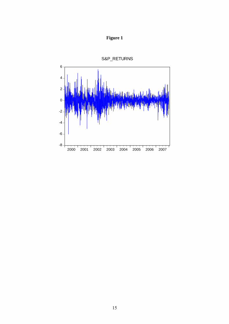
[Insert Figure 1 around here]
Figure 1 shows the Standard and Poor’s returns. The series exhibit clustering, which
could be captured by an appropriate time series model. The descriptive statistics for the
index returns are given in Table 2. The mean is close to zero, and the range is between –
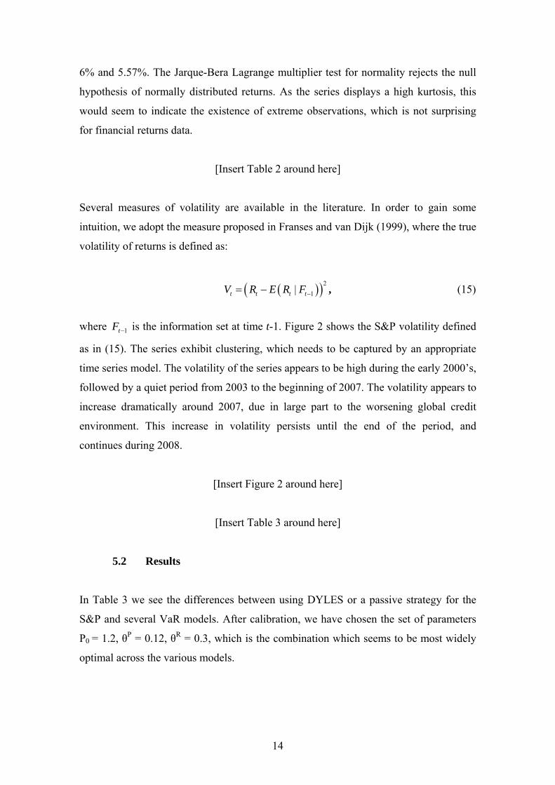
14
6% and 5.57%. The Jarque-Bera Lagrange multiplier test for normality rejects the null
hypothesis of normally distributed returns. As the series displays a high kurtosis, this
would seem to indicate the existence of extreme observations, which is not surprising
for financial returns data.
[Insert Table 2 around here]
Several measures of volatility are available in the literature. In order to gain some
intuition, we adopt the measure proposed in Franses and van Dijk (1999), where the true
volatility of returns is defined as:
( )( )21| −= −t t t tV R E R F , (15)
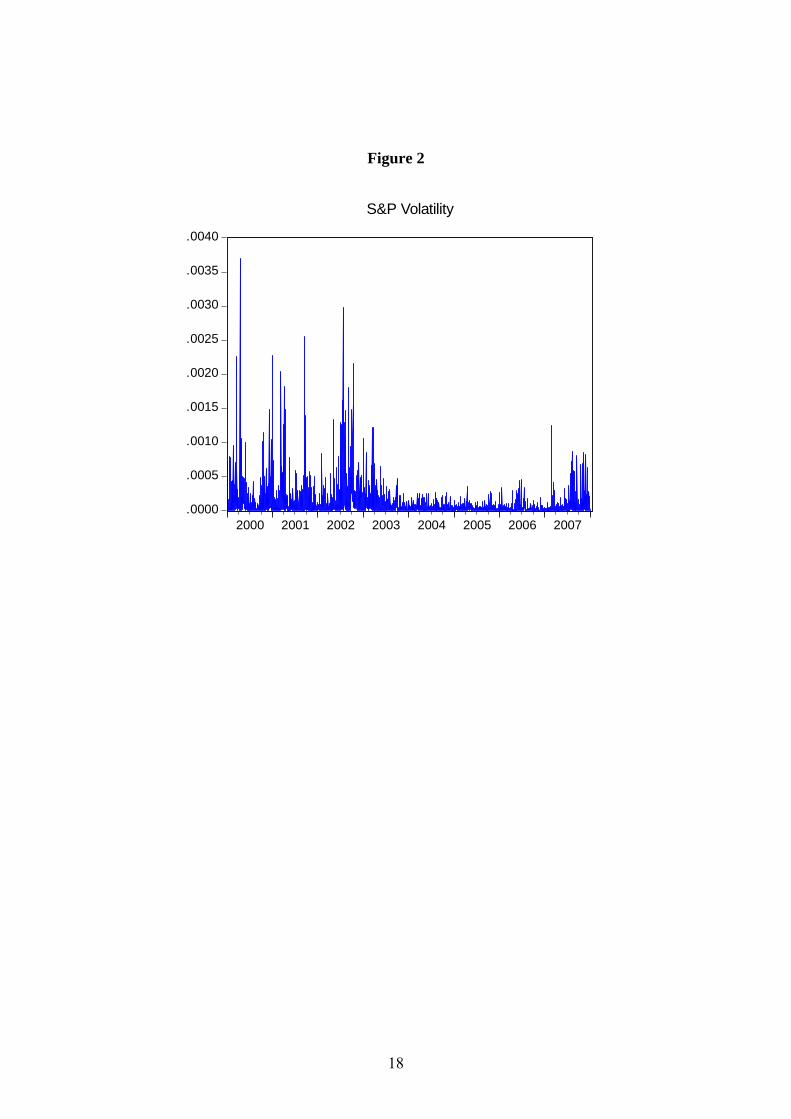
where 1−tF is the information set at time t-1. Figure 2 shows the S&P volatility defined
as in (15). The series exhibit clustering, which needs to be captured by an appropriate
time series model. The volatility of the series appears to be high during the early 2000’s,
followed by a quiet period from 2003 to the beginning of 2007. The volatility appears to
increase dramatically around 2007, due in large part to the worsening global credit
environment. This increase in volatility persists until the end of the period, and
continues during 2008.
[Insert Figure 2 around here]
[Insert Table 3 around here]
5.2 Results
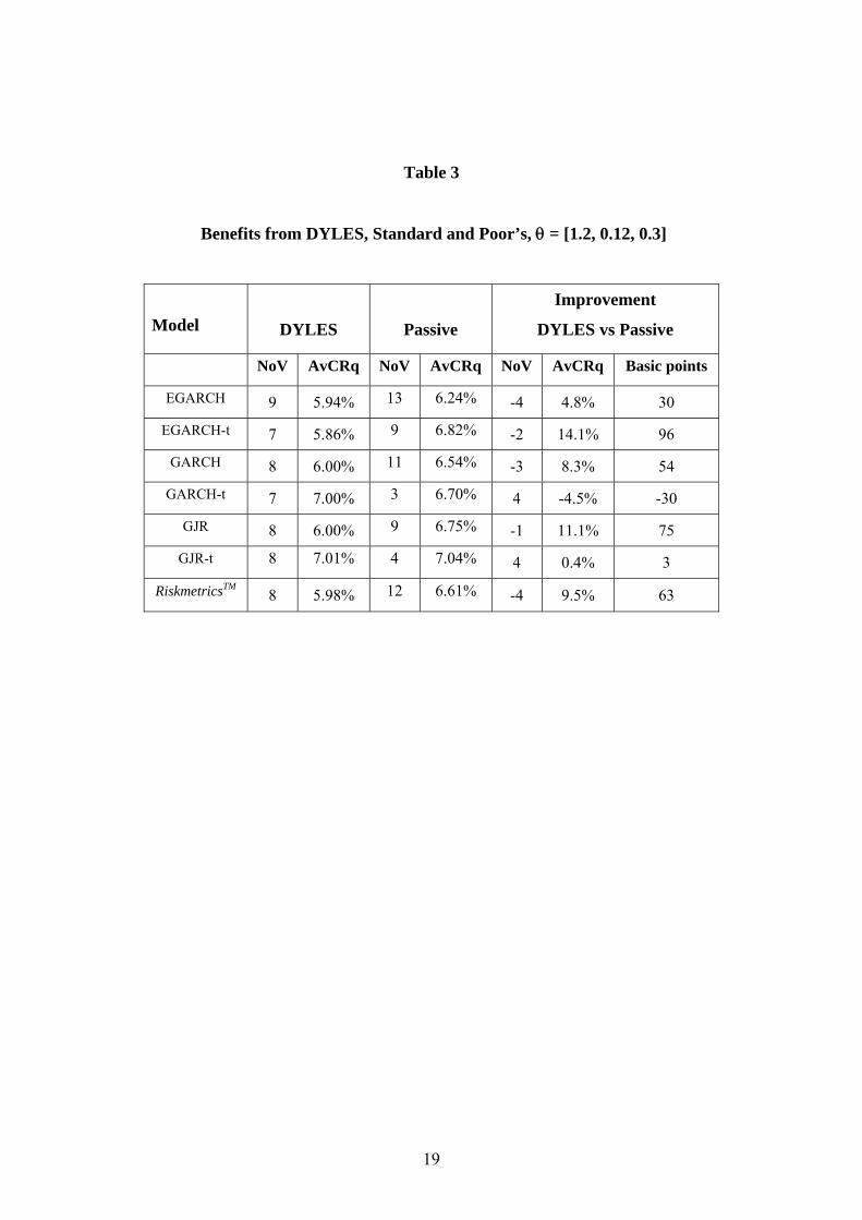
In Table 3 we see the differences between using DYLES or a passive strategy for the
S&P and several VaR models. After calibration, we have chosen the set of parameters
P0 = 1.2, θP = 0.12, θR = 0.3, which is the combination which seems to be most widely
optimal across the various models.
15
Figure 1
-8
-6
-4
-2
0
2
4
6
2000 2001 2002 2003 2004 2005 2006 2007
S&P_RETURNS
16
Table 2
0
100
200
300
400
500
600
-6 -4 -2 0 2 4 6
Series: SP_RETURNSSample 3/01/2000 18/01/2008Observations 2086
Mean 0.000431Median 0.001107Maximum 5.573610Minimum -6.004513Std. Dev. 1.094369Skewness 0.048622Kurtosis 5.760783
Jarque-Bera 663.2940Probability 0.000000
17
We observe in the last column that the capital requirement decreases in all cases
between 0.4% (3 basis points) and 14.01% (96 basis points) when using DYLES, except
when the GARCH-t model is used. Moreover, the number of violations decreases when
they were above 10 and increases, within the limits, when there are few violations. The
exception in Table 4 in the Appendix shows that the best result for the GARCH-t model
and DYLES is for Θ = [1.0, 0.11, 0.3] with 9 violations and 5.80% as AvCRq, that is,
90 basis points less than the no strategy policy.
We conclude that DYLES always beats the passive strategy when properly calibrated.
Due to its context-sensitive behaviour, DYLES tends to concentrate the distribution of
the number of violations. In cases where there is conservative behaviour, it tends to
increase the number of violations, whereas when the number of violations is large, it
tends to reduce it to below the limit of 10.
When properly used, DYLES can decrease the daily capital requirements substantially,
up to 96 basis points in the case analyzed above, while restricting the number of
violations to within the limits of the Basel II Accord.
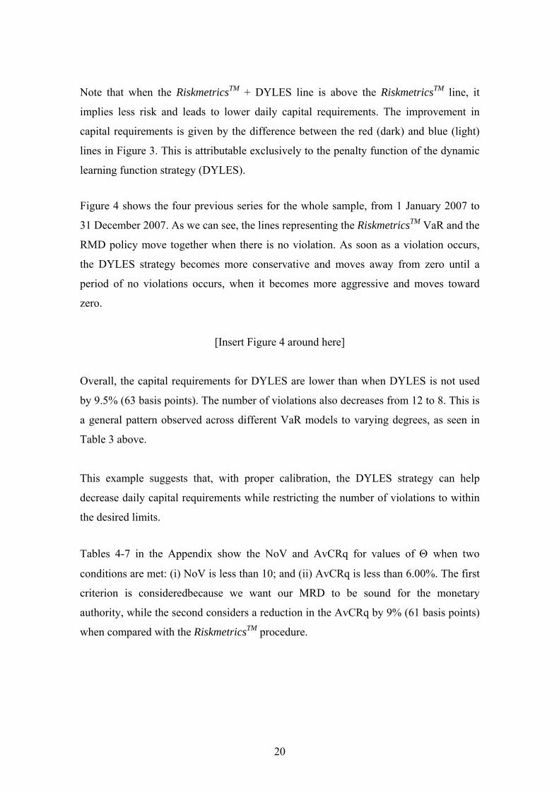
[Insert Figure 3 around here]
In order to gain some intuition, in Figure 3 we present a comparison of DYLES with the
results for RiskmetricsTM.
a. The returns data are for the Standard and Poor’s index during the last 100 days
of 2007.
b. The stepwise line corresponds to the values of DYLES (Pt) during the period for
which Θ = [1.2, 0.12, 0.3].
c. Of the two bottom lines, the one that starts higher is the VaR calculated by
RiskmetricsTM
d. Of the two bottom lines, the one (line with symbols) that starts lower (with
greater risk) is the VaR of RiskmetricsTM + DYLES, which is our RMD.
18
Figure 2
.0000
.0005
.0010
.0015
.0020
.0025
.0030
.0035
.0040
2000 2001 2002 2003 2004 2005 2006 2007
S&P Volatility
19
Table 3
Benefits from DYLES, Standard and Poor’s, θ = [1.2, 0.12, 0.3]
Model
DYLES
Passive
Improvement
DYLES vs Passive
NoV AvCRq NoV AvCRq NoV AvCRq Basic points
EGARCH 9 5.94% 13 6.24% -4 4.8% 30
EGARCH-t 7 5.86% 9 6.82% -2 14.1% 96
GARCH 8 6.00% 11 6.54% -3 8.3% 54
GARCH-t 7 7.00% 3 6.70% 4 -4.5% -30
GJR 8 6.00% 9 6.75% -1 11.1% 75
GJR-t 8 7.01% 4 7.04% 4 0.4% 3
RiskmetricsTM 8 5.98% 12 6.61% -4 9.5% 63
20
Note that when the RiskmetricsTM + DYLES line is above the RiskmetricsTM line, it
implies less risk and leads to lower daily capital requirements. The improvement in
capital requirements is given by the difference between the red (dark) and blue (light)
lines in Figure 3. This is attributable exclusively to the penalty function of the dynamic
learning function strategy (DYLES).
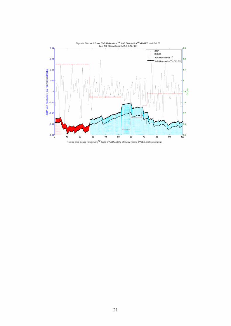
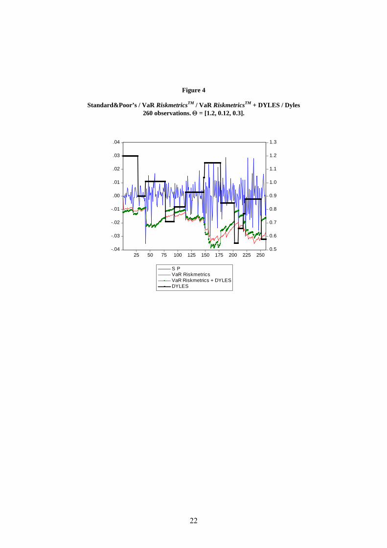
Figure 4 shows the four previous series for the whole sample, from 1 January 2007 to
31 December 2007. As we can see, the lines representing the RiskmetricsTM VaR and the
RMD policy move together when there is no violation. As soon as a violation occurs,
the DYLES strategy becomes more conservative and moves away from zero until a
period of no violations occurs, when it becomes more aggressive and moves toward
zero.
[Insert Figure 4 around here]
Overall, the capital requirements for DYLES are lower than when DYLES is not used
by 9.5% (63 basis points). The number of violations also decreases from 12 to 8. This is
a general pattern observed across different VaR models to varying degrees, as seen in
Table 3 above.
This example suggests that, with proper calibration, the DYLES strategy can help
decrease daily capital requirements while restricting the number of violations to within
the desired limits.
Tables 4-7 in the Appendix show the NoV and AvCRq for values of Θ when two
conditions are met: (i) NoV is less than 10; and (ii) AvCRq is less than 6.00%. The first
criterion is consideredbecause we want our MRD to be sound for the monetary
authority, while the second considers a reduction in the AvCRq by 9% (61 basis points)
when compared with the RiskmetricsTM procedure.
21
0 10 20 30 40 50 60 70 80 90 100-0.04
-0.03
-0.02
-0.01
0
0.01
0.02
0.03
0.04S
&P
, V
aR R
iskm
etric
s, V
ar R
iskm
etric
s+D
YLE
S
Figure 3. Standard&Poors, VaR RiskmetricsTM, VaR RiskmetricsTM +DYLES, and DYLESLast 100 observations Θ=[1.2, 0.12, 0.3]
The red-area means RiskmetricsTM beats DYLES and the blue-area means DYLES beats no strategy
0 10 20 30 40 50 60 70 80 90 1000.5
0.6
0.7
0.8
0.9
1
1.1
1.2
1.3
DY
LES
S&PDYLES
VaR RiskmetricsTM
VaR RiskmericsTM+DYLES
22
Figure 4
Standard&Poor’s / VaR RiskmetricsTM / VaR RiskmetricsTM + DYLES / Dyles
260 observations. Θ = [1.2, 0.12, 0.3].
-.04
-.03
-.02
-.01
.00
.01
.02
.03
.04
0.5
0.6
0.7
0.8
0.9
1.0
1.1
1.2
1.3
25 50 75 100 125 150 175 200 225 250
S PVaR RiskmetricsVaR Riskmetrics + DYLESDYLES
23
Based on Tables 4-7 and the previous analysis, we conclude that there are combinations
of parameters in Θ that can reduce the daily capital requirements compared with
existing models and strategies, while producing an acceptable number of violations. It
would seem to be straightforward to find a parameter vector Θ with a systematically
smaller AvCRq and NoV below 10 for all the models, when compared with the no
strategy policy.
It is noteworthy that, while VaR is used by numerous financial institutions, it is not
without shortcomings. The VaR measure can under or overestimate risk. There is even
debate as to how best to model the behaviour of volatility in market returns. Relying on
DYLES, which modulates market risk disclosure, can reduce the effects of these
deficiencies, as DYLES concentrates NoV throughout the models tested. In some of the
cases discussed above, DYLES can control the number of violations at low cost in terms
of the daily capital requirements.
6. Conclusion
Under the Basel II Accord, ADIs have to communicate their risk estimates to the
monetary authorities, and use a variety of VaR models to estimate risks. ADIs are
subject to a back-test that compares the daily VaR to the subsequent realized returns,
and ADIs that fail the back-test can be subject to the imposition of standard models that
can lead to higher daily capital costs. Additionally, the Basel II Accord stipulates that
the daily capital charge that the bank must carry as protection against market risk must
be set at the higher of the previous day’s VaR or the average VaR over the last 60
business days, multiplied by a factor k. An ADI’s objective is to maximize profits, so
they wish to minimize their capital charges while restricting the number of violations in
a given year below the maximum of 10 allowed by the Basel II Accord.
VaR models currently in use can lead to high daily capital requirements or an excessive
number of violations. In this paper we proposed a new dynamic learning strategy,
DYLES, designed to minimize the daily capital requirements, while restricting the
number of violations to below the penalty limit. We designed a market risk disclosure
strategy driven by the number of violations to communicate the risk to the monetary
authority. The strategy is context sensitive, and depends on the history of violations. It
24
is intended to penalize VaR models when a loss exceeds the reported VaR by increasing
the risk for the following periods. On the other hand, after a given period with no
violations, the criterion offers a reward by decreasing the reported risk.
In order to illustrate the practicability of DYLES, we applied it to the Standard and Poor
500 Index using seven different VaR models. After estimation of the VaR models and
calibration of the parameters, we showed that it could lower the daily capital
requirements substantially (by up to 14.3%, or 95 basis points, when we compared, for
example, the GJR-t model + DYLES to the no strategy RiskmetricsTM policy), while
restricting the numbers of violations to within the Basel II Accord limits (9 for GJR-t +
DYLES and 12 for the no strategy RiskmetricsTM policy ).
Simplicity would seem to have been the key to the popularity of VaR, particularly as a
means of providing information to an ADI’s senior management. DYLES is as simple
and intuitive as VaR. When there is a violation, it increases immediately, thereby
becoming more conservative and decreasing the risks of further violations, whereas
after a period of no violations, it becomes less conservative, thereby allowing lower
daily capital requirements.
The preceding arguments suggest that DYLES can be used profitably by ADIs to reduce
their average daily capital requirements, while restricting the numbers of violations to
the Basel II Accord penalty limits.
25
References
Basel Committee on Banking Supervision, (1988), International Convergence of Capital
Measurement and Capital Standards, BIS, Basel, Switzerland.
Basel Committee on Banking Supervision, (1995), An Internal Model-Based Approach
to Market Risk Capital Requirements, BIS, Basel, Switzerland.
Basel Committee on Banking Supervision, (1996), Supervisory Framework for the Use
of “Backtesting” in Conjunction with the Internal Model-Based Approach to
Market Risk Capital Requirements, BIS, Basel, Switzerland.
Berkowitz, J. and J. O'Brien (2001), How accurate are value-at-risk models at
commercial banks?, Discussion Paper, Federal Reserve Board.
Bollerslev, T. (1986), Generalised autoregressive conditional heteroscedasticity, Journal
of Econometrics, 31, 307-327.
Engle, R.F. (1982), Autoregressive conditional heteroscedasticity with estimates of the
variance of United Kingdom inflation, Econometrica, 50, 987-1007.
Franses, P.H. and D. van Dijk (1999), Nonlinear Time Series Models in Empirical
Finance, Cambridge, Cambridge University Press.
Gizycki, M. and N. Hereford (1998), Assessing the dispersion in banks’ estimates of
market risk: the results of a value-at-risk survey, Discussion Paper 1, Australian
Prudential Regulation Authority.
Glosten, L., R. Jagannathan and D. Runkle (1992), On the relation between the expected
value and volatility of nominal excess return on stocks, Journal of Finance, 46,
1779-1801.
Jorion, P. (2000), Value at Risk: The New Benchmark for Managing Financial Risk,
McGraw-Hill, New York.
Li, W.K., S. Ling and M. McAleer (2002), Recent theoretical results for time series
models with GARCH errors, Journal of Economic Surveys, 16, 245-269.
Reprinted in M. McAleer and L. Oxley (eds.), Contributions to Financial
Econometrics: Theoretical and Practical Issues, Blackwell, Oxford, 2002, pp. 9-
33.
Ling, S. and M. McAleer (2002a), Stationarity and the existence of moments of a family
of GARCH processes, Journal of Econometrics, 106, 109-117.
26
Ling, S. and M. McAleer (2002b), Necessary and sufficient moment conditions for the
GARCH(r,s) and asymmetric power GARCH(r, s) models, Econometric Theory,
18, 722-729.
Ling, S. and M. McAleer, (2003a), Asymptotic theory for a vector ARMA-GARCH
model, Econometric Theory, 19, 278-308.
Ling, S. and M. McAleer (2003b), On adaptive estimation in nonstationary ARMA
models with GARCH errors, Annals of Statistics, 31, 642-674.
McAleer, M. (2005), Automated inference and learning in modeling financial volatility,
Econometric Theory, 21, 232-261.
McAleer, M. (2008), The Ten Commandments for optimizing value-at-risk and daily
capital charges, to appear in Journal of Economic Surveys.
McAleer, M., F. Chan and D. Marinova (2007), An econometric analysis of asymmetric
volatility: theory and application to patents, Journal of Econometrics, 139, 259-
284.
McAleer, M. and B. da Veiga (2008a), Forecasting value-at-risk with a parsimonious
portfolio spillover GARCH (PS-GARCH) model, Journal of Forecasting, 27, 1-19.
McAleer, M. and B. da Veiga (2008b), Single index and portfolio models for
forecasting value-at-risk thresholds, Journal of Forecasting, 27, 217-235.
Nelson, D.B. (1991), Conditional heteroscedasticity in asset returns: a new approach,
Econometrica, 59, 347-370.
RiskmetricsTM (1996), J.P. Morgan Technical Document, 4th Edition, New York, J.P.
Morgan.
Stahl, G. (1997), Three cheers, Risk, 10, 67-69.
27
Appendix 1
Table 1: Basel Accord Penalty Zones
Zone Number of Violations Increase in k
Green 0 to 4 0.00
Yellow 5 0.40
6 0.50
7 0.65
8 0.75
9 0.85
Red 10+ 1.00
Note: The number of violations is given for 250 business days.
The penalty structure under the Basel II Accord is specified for
the number of penalties and not their magnitude, either
individually or cumulatively.
28
Table 4
MRD results when NoV < = 10 and CRq < 6.1%
EGARCH EGARCH-t
NoV AvCRq P0 θP θR NoV AvCRq P0 θP θR
7 5.97% 0.9 0.10 0.1 9 5.91% 0.8 0.11 0.3
9 5.91% 0.9 0.12 0.3 9 5.94% 1.1 0.06 0.2
9 6.00% 1.0 0.10 0.3 9 5.95% 1.1 0.11 0.3
9 5.70% 1.2 0.06 0.2 9 5.87% 1.2 0.09 0.3
9 5.91% 1.2 0.07 0.2 8 5.70% 1.2 0.11 0.3
7 5.93% 1.2 0.10 0.2 7 5.86% 1.2 0.12 0.3
9 5.94% 1.2 0.12 0.3
Table 5
MRD results when NoV < = 10 and CRq < 6.1%
GARCH GARCH-t
NoV AvCRq P0 θP θR NoV AvCRq P0 θP θR
9 5.89% 0.8 0.11 0.3 7 6.00% 0.9 0.11 0.2
9 5.93% 1.1 0.11 0.3 9 5.80% 1.0 0.11 0.3
8 5.85% 1.2 0.11 0.3 8 5.87% 1.1 0.11 0.3
29
Table 6
MRD results when NoV < = 10 and CRq < 6.1%
GJR GJR-t
NoV AvCRq P0 θP θR NoV AvCRq P0 θP θR
9 5.85% 0.6 0.11 0.2 8 6.00% 0.6 0.10 0.2
9 5.92% 1.1 0.06 0.2 8 5.90% 1.0 0.07 0.2
9 5.92% 1.1 0.12 0.3 9 5.66% 1.0 0.12 0.3
9 5.87% 1.2 0.11 0.3 9 5.90% 1.1 0.10 0.3
Table 7
MRD results when NoV < = 10 and CRq < 6.1%
RiskmetricsTM
NoV AvCRq P0 θP θR
9 5.81% 0.8 0.11 0.3
8 5.76% 1.2 0.11 0.3
8 5.98% 1.2 0.12 0.3
Recommended