Diss. ETH Nr. 17760
Impulsive Optimal Control of Hybrid
Finite-Dimensional Lagrangian Systems
A dissertation submitted to the
ETH ZURICH
for the Degree of
Doctor of Technical Sciences
presented by
Kerim Yunt
M. Sc. Systems and Control Engineer
Bogazici University/ Istanbul
born October 21, 1973
citizen of Turkey
accepted on the recommendation of
Prof. Dr.-Ing. Dr.-Ing. habil. Ch. Glocker, examiner
Prof. Dr. Dipl.-Ing. L. Guzzella, co-examiner
2008

ii
.

iii
Abstract
The scope of this dissertation addresses numerical and theoretical issues in the impulsive
control of hybrid finite-dimensional Lagrangian systems. In order to treat these aspects, a mod-
eling framework is presented based on the measure-differential inclusion representation of the
Lagrangian dynamics. The main advantage of this representation is that it enables the incor-
poration of set-valued force laws and control laws on acceleration and velocity level concisely.
This property of the measure-differential inclusion representation renders the description of the
hybrid behaviour of Lagrangian systems in the framework of set-valued control and force laws
possible. Based on the MDI representation of Lagrangian dynamics the impactive blocking
is analysed as a set-valued impulsive unbounded control law. The application to mechanical
systems with impulsively-blockable degrees of freedom is presented. The numerical application
of this set-valued control law is the formulation of a nonlinear programming (NLP) algorithm
for underactuated mechanical systems with impulsively-blockable DOF. The natural numerical
treatment of the measure-differential inclusion representation is based on Moreau’s sweeping
process. By applying this discretisation scheme together with an augmented Lagrangian based
NLP method that performs the minimisations with a modified conjugate gradients method an
optimisation scheme is presented. A numerical example is applied to the impulsive optimal
control of a manipulator with one impulsively-blockable degrees of freedom. A further numeri-
cal method is introduced for the class of switching Lagrangian systems. This numerical method
is a shooting method that performs the numerical integrations based on the sweeping process
and the minimisations by making use of the augmented Lagrangian concept. The augmented
Lagrangian is minimised by an optimisation method that relies on function value comparisons.
This relatively easily implemented numerical method is applied to a wheeled robot which is
a tenth-order dynamical system. This system has four different operating modes and time
and control effort (quasi-) optimal trajectories are presented. The theoretical results of the
dissertation include the statement and the derivation of necessary conditions for the impulsive
optimal control of finite-dimensional Lagrangian systems. In this analysis, Lagrangian systems
are considered on which the impulses are induced solely by the impulsive control action. The
challenge in the derivation of these necessary conditions has been the concurrent discontinuity
of state and costate on a Lebesgue negligible time instant. In order to tackle this problem,
the instances of impulsive control action are considered as an internal boundaries on the time
domain. By the introduction of the concepts of internal boundary variations and discontinuous
transversality conditions by the author this problem is resolved and necessary conditions for
mechanical systems in the first-order and second-order representations are derived. The discon-
tinuous transversality conditions that result from the consideration of the internal boundary
variations in the time domain are discovered and analysed by the author of the dissertation
and are applied to the impulsive optimal control of Lagrangian systems.

iv
.

v
Zusammenfassung
Im Rahmen dieser Dissertation wurden numerische und theoretische Problemstellungen im
Bereich der impulsiven Steuerung hybrider endlich-dimensionaler Lagrangescher Systeme be-
handelt. In der Behandlung der Problemstellungen wurde die dynamische Modellierung auf
das mathematische Konzept der Massdifferentialinklusionen (MDI) basiert. Das Konzept der
Massdifferentialinklusion ermoglicht die einwandfreie und prazise Eingliederung von mengen-
wertigen Steuer-, und Kraftgesetzen im Modell. Diese Eigenschaft der MDI Darstellung ist der
Hauptvorteil und ermoglicht die Beschreibung des hybriden Verhaltens Lagrangescher Systeme
mit Hilfe von mengenwertigen Kraft und Steuergesetzen. Basierend auf die MDI Darstellung
der Lagrangeschen Dynamik wird die stosshafte Blockierung analysiert und als ein mengen-
wertiges unbregenztes impulsives Steuergesetz eingefuhrt. Die Anwendung dieses Steuerge-
setzes auf mechanische Systeme mit stosshaft blockierbaren Freiheitsgraden wird prasentiert.
Als numerische Anwendung des mengenwertigen Steuergesetzes in der impulsiven optimalen
Steuerung wird ein nichtlinearer Programmierungsalgorithmus (NLP) beschrieben, der die Bes-
timmung optimaler Trajektorien fur unteraktuierte Lagrangesche Systeme mit stosshaft block-
ierbaren Gelenken bezweckt. Die naturliche numerische Behandlung der Massdifferentialinklu-
sionen basiert auf dem Sweeping Algorithmus von Moreau. Der NLP-Algorithmus vereinigt in
sich das Diskretisierungsschema des Sweeping Algorithmuses und die erweiterte Lagrangesche
Methode in Optimierung. Die Minimierung der erweiterten Lagrangeschen Funktion wird mit
einem modifizierten konjugierten Gradientenverfahren bewaltigt. Ein numerisches Beispiel wird
angefuhrt, das die numerische Ermittlung der impulsiven optimalen Steuerung eines Manipu-
lators mit einem stosshaft blockierbaren Gelenk beschreibt. Im weiteren wird eine numerische
Methode vorgestellt, das ein Schiessverfahren ist, in der die numerische Integration mit dem
Sweeping Algorithmus ausgefuhrt wird. Dieses Schiessverfahren ermoglicht die Bestimmung op-
timaler Trajektorien von einer bestimmten Klasse von Lagrangeschen Systemen, die im Rahmen
dieser Arbeit umschaltende Lagrangesche Systeme genannt werden. Die zugehorige erweiterte
Lagrangesche Funktion wird mittels eines Optimierungsverfahrens minimiert, das auf Funktion-
swertvergleich beruht. Die im Vergleich zu NLP Methoden relativ einfach implementierbare
Methode wird zur optimalen Trajektorienbestimmung eines Roboters mit Radern angewendet,
der als ein dynamisches System zehnter Ordnung beschrieben wird. Dieses System hat vier
Moden, die sich voneinander aufgrund des Haft-Gleit Zustandes der Rader unterscheiden. Zeit
und steuerungsaufwandsoptimierte Trajektorien werden prasentiert.
Der theoretische Beitrag der Arbeit ist die Bestimmung der notwendigen Bedingungen fur
impulsive optimale Steuerungen endlich-dimensionaler Lagrangescher Systeme. In der Anal-
yse wird angenommen, dass die impulsive Steuerung die einzige stosshafte Anregung des La-
grangeschen Systems darstellt. Die Herausforderung in der Herleitung der notwendigen Bedin-
gungen ist die Behandlung der gleichzeitigen Unstetigkeit in den Geschwindigkeiten des mecha-

vi
nischen Systems und der adjungierten Zustanden. Um diese Herausforderung zu meistern wur-
den die Momente der impulsiven Steuerungseingriffe als innere Grenzen im Zeitbereich betra-
chtet. Der Verfasser dieser Dissertation fuhrt deswegen die Variationen an den inneren Randern
im Zeitbereich zusammen mit den diskontinuierlichen Transversalitatsbedingungen ein, um
diese Komplikation zu beheben. Auf diesen diskontinuierlichen Transversalitatsbedingungen
basierend wurden notwendige Bedingungen in erster und zweiter Ordnungsdarstellung hergeleitet,
die von einer optimalen Bahn erfullt werden mussen. Die aus den inneren Randvariationen
hervorgehenden diskontinuierlichen Transversalitatsbedingungen wurden vom Verfasser dieser
Dissertation in eigenstandiger Arbeit erfunden, analysiert und auf impulsive Steuerung La-
grangescher Systeme angewendet.

vii
Acknowledgements
I want to thank all friends and colleagues in the center of mechanics who supported me
during my work at the institute, provided me the necessary means and research environment
to conduct my research for which I am still very enthusiatic to continue. At this point, I
want to express my gratitude to Professor Christoph Glocker who enabled to work on this very
interesting field of research. My dear family deserves the greatest thanks for making me the
person who I am and shaping my personality over the decades. My heart goes with Daniela
Tanner when I think how much she cared for me in the final phases of writing. And when I
think about all the things we went through together, my love for her grows larger.

viii
.

Contents
1 Introduction 1
1.1 Modeling . . . . . . . . . . . . . . . . . . . . . . . . . . . . . . . . . . . . . . . . 3
1.2 Optimal Control and Hybrid Systems . . . . . . . . . . . . . . . . . . . . . . . . 5
1.3 Discontinuous Transversality Conditions . . . . . . . . . . . . . . . . . . . . . . 8
1.4 Numerical Analysis . . . . . . . . . . . . . . . . . . . . . . . . . . . . . . . . . . 10
2 Modeling of Hybrid FDLS 19
2.1 Preliminaries . . . . . . . . . . . . . . . . . . . . . . . . . . . . . . . . . . . . . 19
2.2 Lagrange Equations in Impulsive Control Form . . . . . . . . . . . . . . . . . . 23
2.3 The MDI of Motion for FDLS with Controls . . . . . . . . . . . . . . . . . . . . 25
2.3.1 LCP Representation of MDI . . . . . . . . . . . . . . . . . . . . . . . . . 27
2.3.2 Impact Equation . . . . . . . . . . . . . . . . . . . . . . . . . . . . . . . 31
2.4 Underactuated Manipulators with Impactive Blocking . . . . . . . . . . . . . . . 35
2.5 Complementarity Description of Impulsive Blocking . . . . . . . . . . . . . . . . 36
2.5.1 A Case Study . . . . . . . . . . . . . . . . . . . . . . . . . . . . . . . . . 43
2.6 Impactive Underactuated Manipulators . . . . . . . . . . . . . . . . . . . . . . . 45
2.6.1 Post-transition State and Discontinuity . . . . . . . . . . . . . . . . . . . 45
2.6.2 Lagrangian Dynamics in Different Phases of Motion . . . . . . . . . . . . 48
2.6.3 Change in Mechanical Energy and Impuls and Dissipation . . . . . . . . 50
2.6.4 Example: Planar Double Pendulum with One Blockable DOF . . . . . . 51
3 Numerical Methods for FDLS 55
3.1 Preliminaries . . . . . . . . . . . . . . . . . . . . . . . . . . . . . . . . . . . . . 58
3.1.1 Complementarity Problems and Variational Inequalities . . . . . . . . . . 67
3.2 Properties of the Augmented Lagrangian Method . . . . . . . . . . . . . . . . . 72
3.2.1 The Lagrangian and the Augmented Lagrangian . . . . . . . . . . . . . . 72
3.2.2 Normality and Degeneracy of the NLP Problem . . . . . . . . . . . . . . 75
3.2.3 Local Analysis of the Augmented Lagrangian Function . . . . . . . . . . 78
3.2.4 Global Analysis of the Augmented Lagrangian Function . . . . . . . . . . 81
ix

x CONTENTS
3.2.5 Comparison of Strategies . . . . . . . . . . . . . . . . . . . . . . . . . . . 84
3.3 NLP Method for MPEC . . . . . . . . . . . . . . . . . . . . . . . . . . . . . . . 86
3.3.1 The Transcription of a mechanical MDI Optimal Control Problem into a
NLP . . . . . . . . . . . . . . . . . . . . . . . . . . . . . . . . . . . . . . 89
3.3.2 Formulas for the Determination of the Numerical Gradient of the Aug-
mented Lagrangian . . . . . . . . . . . . . . . . . . . . . . . . . . . . . . 93
3.3.3 The NLP Algorithm . . . . . . . . . . . . . . . . . . . . . . . . . . . . . 95
3.3.4 Implementation of the Algorithm . . . . . . . . . . . . . . . . . . . . . . 99
3.4 Numerical Example . . . . . . . . . . . . . . . . . . . . . . . . . . . . . . . . . . 99
3.4.1 Case A . . . . . . . . . . . . . . . . . . . . . . . . . . . . . . . . . . . . . 103
3.4.2 Case B . . . . . . . . . . . . . . . . . . . . . . . . . . . . . . . . . . . . . 110
3.4.3 Case C . . . . . . . . . . . . . . . . . . . . . . . . . . . . . . . . . . . . . 116
3.5 Augmented Lagrangian based Shooting Method . . . . . . . . . . . . . . . . . . 124
3.6 Contact Dynamics and Integration . . . . . . . . . . . . . . . . . . . . . . . . . 126
3.6.1 Formulation of Shooting Method . . . . . . . . . . . . . . . . . . . . . . 129
3.7 Model of the Diff-Drive Robot . . . . . . . . . . . . . . . . . . . . . . . . . . . . 131
3.7.1 Determination of Normal Contact Force Differential Measures . . . . . . 136
3.8 Numerical Results . . . . . . . . . . . . . . . . . . . . . . . . . . . . . . . . . . . 139
3.8.1 Case A . . . . . . . . . . . . . . . . . . . . . . . . . . . . . . . . . . . . . 140
3.8.2 Case B . . . . . . . . . . . . . . . . . . . . . . . . . . . . . . . . . . . . . 140
3.8.3 Case C . . . . . . . . . . . . . . . . . . . . . . . . . . . . . . . . . . . . . 141
3.8.4 Case D . . . . . . . . . . . . . . . . . . . . . . . . . . . . . . . . . . . . . 148
3.8.5 Simplectic and Dissipative Properties of the Sweeping Process . . . . . . 150
3.8.6 Convergence Behaviour of Case B . . . . . . . . . . . . . . . . . . . . . . 153
4 Discontinuous Transversality and Impulsive Control 157
4.1 Introduction . . . . . . . . . . . . . . . . . . . . . . . . . . . . . . . . . . . . . . 157
4.2 Preliminaries . . . . . . . . . . . . . . . . . . . . . . . . . . . . . . . . . . . . . 159
4.2.1 Regularity of Sets . . . . . . . . . . . . . . . . . . . . . . . . . . . . . . . 162
4.3 Impulsive Generalised Problem of Bolza . . . . . . . . . . . . . . . . . . . . . . 164
4.4 Statement of the Optimal Control Problem . . . . . . . . . . . . . . . . . . . . . 166
4.5 Discontinuous Transversality Conditions . . . . . . . . . . . . . . . . . . . . . . 171
4.5.1 Internal Boundary Variations . . . . . . . . . . . . . . . . . . . . . . . . 172
4.5.2 Discontinuous Transversality Conditions . . . . . . . . . . . . . . . . . . 173
4.5.3 Total Directional Derivatives of The Value Function J . . . . . . . . . . . 179
4.6 Necessary Conditions . . . . . . . . . . . . . . . . . . . . . . . . . . . . . . . . . 180
4.7 Necessary Conditions for Impactive Underactuated Systems . . . . . . . . . . . 183

CONTENTS xi
5 Hamiltonian Approach 185
5.1 Derivation of First-order Conditions . . . . . . . . . . . . . . . . . . . . . . . . . 185
5.2 Generalised Problem of Bolza . . . . . . . . . . . . . . . . . . . . . . . . . . . . 186
5.3 Statement of IOC . . . . . . . . . . . . . . . . . . . . . . . . . . . . . . . . . . . 189
5.4 Necessary Conditons . . . . . . . . . . . . . . . . . . . . . . . . . . . . . . . . . 197
5.5 Case Study . . . . . . . . . . . . . . . . . . . . . . . . . . . . . . . . . . . . . . 199
6 Discussion and Conclusion 203
6.1 Results on Numerical Methods . . . . . . . . . . . . . . . . . . . . . . . . . . . . 203
6.2 Variational Results . . . . . . . . . . . . . . . . . . . . . . . . . . . . . . . . . . 208
Bibliography 211
Curriculum Vitae 222

xii CONTENTS
.

CONTENTS xiii
List of Symbols
< Elementwise greater equal than
4 Elementwise less equal than
| · | Absolute value of the argument
∇x y Gradient of y w.r.t x
A ⊂ B A is subset of BA ⊃ B A is superset of BN(B) Number of elements of set B〈·, ·〉 scalar product or dual pairing of the arguments
a× b cross product of vectors a and b
a⊥b Scalar product of a and b is zero
B Open unit ball in Euclidean space
|x| Euclidean norm of x
dC(x) Euclidean distance of x from Cint C Interior of C
bdy C Boundary of CC Closure of C
N PC (x) Proximal normal cone to C at x
NC(x) Strict normal cone to C at x
NC(x) Limiting normal cone to C at x
∞N PC (x) Singular proximal normal cone to C at x
∞NC(x) Singular strict normal cone to C at x
∞NC(x) Singular limiting normal cone to C at x
TC(x) Bouligand tangent cone to C at x
TC(x) Clarke tangent cone to C at x
epi f Epigraph of f
∂P f(x) Proximal subdifferential of f at x
∂ f(x) Strict subdifferential of f at x
∂ f(x) Limiting subdifferential of f at x
∂∞P f(x) Asymptotic proximal subdifferential of f at x
∂∞P f(x) Asymptotic strict subdifferential of f at x
∂∞ f(x) Asymptotic limiting subdifferential of f at x

xiv CONTENTS
dom f (Effective) domain of f
GrF Graph of Fepi f Epigraph of f
f 0(x;v) Generalised directional derivative of f at x in the direction of v
ΨC(x) Indicator function of the set C at the point x
∇ f(x) Gradient vector of f at x
xi−→C x xi → x and xi ∈ C, ∀ixi−→f x xi → x and f(xi) → f(x), ∀i
supp µ Support of the measure µ
List of Abbreviations
BV(I;Rn) Bounded variation functions f : I → Rn
LCBV(I;Rn) Left-continuous bounded variation functions f : I → Rn
RCBV(I;Rn) Right-continuous bounded variation functions f : I → Rn
LBV(I;Rn) Locally bounded variation functions f : I → Rn
LCLBV(I;Rn) Left-continuous locally bounded variation functions f : I → Rn
RCLBV(I;Rn) Right-continuous locally bounded variation functions f : I → Rn
AC(I;Rn) Absolutely continuous functions f : I → Rn
LCP Linear Complementarity Problem
NCP Nonlinear Complementarity Problem
MCP Mixed Complementarity Problem
MPEC Mathematical Programs with Complementarity Constraints
NLP Nonlinear Programing
TOHLS Trajectory Optimisation of Hybrid Lagrangian Systems
FDLS Finite-Dimensional Lagrangian System
UPR(·) Unilateral primitve
SGN(·) Set-valued Signum Relation

List of Tables
3.1 System parameters of the manipulator for cases A, B, C. . . . . . . . . . . . . . 101
3.2 Correspondence between inequalities and dual multipliers in the NLP of the
planar double pendulum. . . . . . . . . . . . . . . . . . . . . . . . . . . . . . . . 101
3.3 Case A: The mode sequence, duration and intervals of modes. . . . . . . . . . . 105
3.4 Case A: Optimisation parameters, initial and final states of the optimisation. . 105
3.5 Case B: The mode sequence, duration and intervals of modes. . . . . . . . . . . 110
3.6 Case B: Optimisation parameters, initial and final states of the optimisation. . 111
3.7 Case C: The mode sequence, duration and intervals of modes. . . . . . . . . . . 117
3.8 Case C: Optimisation parameters, initial and final states of the optimisation. . 117
3.9 Notation Convention. . . . . . . . . . . . . . . . . . . . . . . . . . . . . . . . . . 132
3.10 The classification of modes by making use of the relative contact state of the rear
wheels (The modes that emanate due to the stick-slide situations of the frontal
contact CF are neglected, µf ≈ 0) . . . . . . . . . . . . . . . . . . . . . . . . . . 134
3.11 Numerical values of physical parameters of the robot. The numerical values are
obtained from the CAD of a real mobile robot. . . . . . . . . . . . . . . . . . . . 137
3.12 Numerical parameters of the optimisations in Maneuvers A, B, C and D. Here
ct and cd are penalties imposed on contraints on end time and on the deviation
from the final state, respectively. . . . . . . . . . . . . . . . . . . . . . . . . . . 140
xv

List of Figures
2.1 Unilateral primitive. . . . . . . . . . . . . . . . . . . . . . . . . . . . . . . . . . 21
2.2 Decomposition of the Signum relation into two Uprs. . . . . . . . . . . . . . . . 21
2.3 General contact kinematics. . . . . . . . . . . . . . . . . . . . . . . . . . . . . . 26
2.4 Decomposition of the set-valued Sgn relation into two Unilateral Primitives. . . 30
2.5 (a) A perfect bilateral constraint is equivalent to a normal control force that
takes infinite values, (b) For values of N less than infinity and greater zero, the
blocking action has friction characteristics, (c) if n = 0 there is no braking force. 38
2.6 The set-valued signum relation and its decomposition into two unilateral prim-
itives that represents relation between the discretised differential measure of
normal blocking force to the discretised differential measure of the control force. 39
2.7 (a) If N rises to infinity, the relative velocity in the next moment drops to zero,
(b) For values of N less than infinity and greater zero, the blocking action has
friction characteristics with respect to the relative velocity, (c) if N = 0 there is
no blocking in the next moment. . . . . . . . . . . . . . . . . . . . . . . . . . . . 40
2.8 The unilateral primitive about the relation of the blocking normal force to the
relative acceleration γ+b . . . . . . . . . . . . . . . . . . . . . . . . . . . . . . . . 40
2.9 The UPR about the relation of the differential measure of blocking normal im-
pulsive force to the relative velocity γ+b ∈ RCLBV . . . . . . . . . . . . . . . . . 40
2.10 The decomposition of the Upr relation in figure 2.9 into two unilateral primitives. 41
2.11 The decomposition of the Upr relation in figure 2.8 into two unilateral primitives. 41
2.12 The 2-DOF linear mechanism . . . . . . . . . . . . . . . . . . . . . . . . . . . . 43
2.13 Planar double pendulum with one impactively blockable degrees of freedom. . . 51
3.1 A nonconvex function f , its epigraph, and the Generalised Subdifferential at x0. 62
3.2 The functions ΦFB and -ΦFB. . . . . . . . . . . . . . . . . . . . . . . . . . . . . 69
3.3 The limiting subdifferentials of ΦFB and -ΦFB at the origin. . . . . . . . . . . . 70
3.4 The decomposition of the Upr relation into two unilateral primitives in discretised
form. . . . . . . . . . . . . . . . . . . . . . . . . . . . . . . . . . . . . . . . . . . 87
xvi

LIST OF FIGURES xvii
3.5 The set-valued signum relation and its decomposition into two unilateral prim-
itives that represents relation between the discretised differential measure of
normal blocking force to the discretised differential measure of the control force
in discretised form. . . . . . . . . . . . . . . . . . . . . . . . . . . . . . . . . . . 88
3.6 The simplified flowchart of the algorithm. . . . . . . . . . . . . . . . . . . . . . . 97
3.7 The flowchart of the conjugate gradients minimisation. . . . . . . . . . . . . . . 98
3.8 The parameters of the planar double pendulum. . . . . . . . . . . . . . . . . . . 100
3.9 Case A: The optimal evolution of the generalised velocities α, β, relative velocity
α− β, generalize positions α, β and relative position α−β. ( red lines mark the
transition times) . . . . . . . . . . . . . . . . . . . . . . . . . . . . . . . . . . . 104
3.10 Case A: Maneuver of the double pendulum (Color code: For link 2 white is
blocked, black is unblocked, for link 1 green position at transition interval). . . . 105
3.11 Case A: The optimal evolution of the discretised differential measures N , Γ, the
torque τ and the slack velocity γbr (red lines mark the transition times). . . . . . 106
3.12 Case A: The numerical residue of the discretised equations of motion approx. byB[k]∆ t
(red lines mark the transition times). . . . . . . . . . . . . . . . . . . . . . . 106
3.13 Case A: Residues of the reformulation functions ΦR, ΦL, ΦNR and ΦNL (red lines
mark the transition times). . . . . . . . . . . . . . . . . . . . . . . . . . . . . . . 107
3.14 Case A: The optimal evolution of the dual multipliers mBLα, m
BLβ, pBLα and p
BLβ
(red lines mark the transition times). . . . . . . . . . . . . . . . . . . . . . . . . 107
3.15 Case A: The time evolution of the costate dynamics in the second-order form
(red lines mark the transition times). . . . . . . . . . . . . . . . . . . . . . . . . 108
3.16 Case A:The optimal evolution of the dual multipliers mLR, mLL, pLR and pLL
(red lines mark the transition times). . . . . . . . . . . . . . . . . . . . . . . . . 108
3.17 Case A: The optimal evolution of the dual multipliers mLNR, mLNL, pLNR andpLNL (red lines mark the transition times). . . . . . . . . . . . . . . . . . . . . . 109
3.18 Case A: The residues of the complementarities (red lines mark the transition
times). . . . . . . . . . . . . . . . . . . . . . . . . . . . . . . . . . . . . . . . . . 109
3.19 Case B: The optimal evolution of the generalised velocities α, β, relative velocity
α− β, generalised positions α, β and relative position α− β. red lines mark the
transition times) . . . . . . . . . . . . . . . . . . . . . . . . . . . . . . . . . . . 111
3.20 Case B: Maneuver of the double pendulum (Color code: For link 2 white is
blocked, black is unblocked, for link 1 green position at transition interval). . . . 112
3.21 Case B: The optimal evolution of the discretised differential measures N , Γ, the
torque τ and the slack velocity γbr (red lines mark the transition times). . . . . . 112
3.22 Case B: The numerical residue of the discretised equations of motion of motion
approx. by B[k]∆ t
(red lines mark the transition times). . . . . . . . . . . . . . . . 113
xviii LIST OF FIGURES
3.23 Case B: Residues of the reformulation functions ΦR, ΦL, ΦNR and ΦNL (red lines
mark the transition times). . . . . . . . . . . . . . . . . . . . . . . . . . . . . . . 113
3.24 Case B: The optimal evolution of the dual multipliers mBLα, m
BLβ, pBLα and p
BLβ
(red lines mark the transition times). . . . . . . . . . . . . . . . . . . . . . . . . 114
3.25 Case B: The time evolution of the costate dynamics in the second-order form
(red lines mark the transition times). . . . . . . . . . . . . . . . . . . . . . . . . 114
3.26 Case B:The optimal evolution of the dual multipliers mLR, mLL, pLR and pLL
(red lines mark the transition times). . . . . . . . . . . . . . . . . . . . . . . . . 115
3.27 Case B:The optimal evolution of the dual multipliers mLNR, mLNL, pLNR andpLNL (red lines mark the transition times). . . . . . . . . . . . . . . . . . . . . . 115
3.28 Case B: The residues of the complementarities (red lines mark the transition
times). . . . . . . . . . . . . . . . . . . . . . . . . . . . . . . . . . . . . . . . . . 116
3.29 Case C: The optimal evolution of the generalised velocities α, β, relative velocity
α − β, generalize positions α, β and relative position α − β. red lines mark the
transition times) . . . . . . . . . . . . . . . . . . . . . . . . . . . . . . . . . . . 118
3.30 Case C:Maneuver of the double pendulum (Color code: For link 2 white is
blocked, black is unblocked, for link 1 green position at transition interval). . . . 119
3.31 Case C: The optimal evolution of the discretised differential measures N , Γ, the
torque τ and the slack velocity γbr (red lines mark the transition times). . . . . . 119
3.32 Case C: The numerical residue of the discretised equations of motion approx. byB[k]∆ t
(red lines mark the transition times). . . . . . . . . . . . . . . . . . . . . . . 120
3.33 Case C: Residues of the reformulation functions ΦR, ΦL, ΦNR and ΦNL (red lines
mark the transition times). . . . . . . . . . . . . . . . . . . . . . . . . . . . . . . 120
3.34 Case C: The optimal evolution of the dual multipliers mBLα, m
BLβ, pBLα and p
BLβ
(red lines mark the transition times). . . . . . . . . . . . . . . . . . . . . . . . . 121
3.35 Case C: The time evolution of the costate dynamics in the second-order form
(red lines mark the transition times). . . . . . . . . . . . . . . . . . . . . . . . . 121
3.36 Case C:The optimal evolution of the dual multipliers mLR, mLL, pLR and pLL
(red lines mark the transition times). . . . . . . . . . . . . . . . . . . . . . . . . 122
3.37 Case C:The optimal evolution of the dual multipliers mLNR, mLNL, pLNR andpLNL (red lines mark the transition times). . . . . . . . . . . . . . . . . . . . . . 122
3.38 Case C: The residues of the complementarities (red lines mark the transition
times). . . . . . . . . . . . . . . . . . . . . . . . . . . . . . . . . . . . . . . . . . 123
3.39 Contact forces and motor moments on the simplified model. . . . . . . . . . . . 132
3.40 The degrees of freedom and coordinate frames of the wheeled robot. . . . . . . . 132
3.41 Case A: Contact forces and contact relative velocities. . . . . . . . . . . . . . . . 141
3.42 Case B: Contact forces and contact relative velocities. . . . . . . . . . . . . . . . 142

LIST OF FIGURES xix
3.43 Case A: Number of DOF during the maneuver. . . . . . . . . . . . . . . . . . . 142
3.44 Case B: Number of DOF during the maneuver. . . . . . . . . . . . . . . . . . . . 142
3.45 Case A: The final time tf during successive minimisations. . . . . . . . . . . . . 143
3.46 Case B: The final time tf during successive minimisations. . . . . . . . . . . . . 143
3.47 Case A: The evolution of the trajectory of the CM. . . . . . . . . . . . . . . . . 143
3.48 Case B: The evolution of the trajectory of the CM. . . . . . . . . . . . . . . . . 143
3.49 Case C: Number of DOF during the maneuver. . . . . . . . . . . . . . . . . . . 143
3.50 Case D: Number of DOF during the maneuver. . . . . . . . . . . . . . . . . . . 143
3.51 Case C: Control Moments and phases of chassis DOF. . . . . . . . . . . . . . . . 144
3.52 Case D: Control Moments and phases of chassis DOF. . . . . . . . . . . . . . . . 144
3.53 Case C: Final time tf . . . . . . . . . . . . . . . . . . . . . . . . . . . . . . . . . . 145
3.54 Case D: Final time tf . . . . . . . . . . . . . . . . . . . . . . . . . . . . . . . . . 145
3.55 Case C: The control effort. . . . . . . . . . . . . . . . . . . . . . . . . . . . . . . 145
3.56 Case D: The control effort. . . . . . . . . . . . . . . . . . . . . . . . . . . . . . . 145
3.57 Case C: Contact forces and contact relative velocities. . . . . . . . . . . . . . . . 145
3.58 Case D: Contact forces and contact relative velocities. . . . . . . . . . . . . . . . 146
3.59 Case C: Contact forces and contact relative velocities. . . . . . . . . . . . . . . . 146
3.60 Case A: Control Moments and phases of chassis DOF. . . . . . . . . . . . . . . . 147
3.61 Case B: Control Moments and phases of chassis DOF. . . . . . . . . . . . . . . . 147
3.62 ∆T jerr for Maneuver A. . . . . . . . . . . . . . . . . . . . . . . . . . . . . . . . . 149
3.63 ∆T jerr for Maneuver B. . . . . . . . . . . . . . . . . . . . . . . . . . . . . . . . . 149
3.64 ∆T jerr for Maneuver C. . . . . . . . . . . . . . . . . . . . . . . . . . . . . . . . . 149
3.65 ∆T jerr for Maneuver D. . . . . . . . . . . . . . . . . . . . . . . . . . . . . . . . . 149
3.66 WC
WDfor Maneuvers in intermediate Optimisation stages. . . . . . . . . . . . . . . 149
3.67 WC + WD for Maneuvers in intermediate Optimisation stages. . . . . . . . . . . 149
3.68 Case A: Errors in Energy. . . . . . . . . . . . . . . . . . . . . . . . . . . . . . . 150
3.69 Case B: Errors in Energy. . . . . . . . . . . . . . . . . . . . . . . . . . . . . . . 150
3.70 Case C: Errors in Energy. . . . . . . . . . . . . . . . . . . . . . . . . . . . . . . 150
3.71 Case D: Errors in Energy. . . . . . . . . . . . . . . . . . . . . . . . . . . . . . . 150
3.72 Case B: Evolution and Convergence Behaviour of x and x trajectories. . . . . . . 153
3.73 Case B: Evolution and Convergence Behaviour of y and y trajectories. . . . . . . 154
3.74 Case B: Evolution and Convergence Behaviour of φ and φ trajectories. . . . . . 154
3.75 Case B: Evolution of ΨR, ΨL, ΨR and ΨL trajectories. . . . . . . . . . . . . . . . 155
3.76 Case B: Evolution and Convergence Behaviour of ML and MR trajectories. . . . 155
3.77 Case B: Evolutions of DOF x,y and φ as phase diagrams. . . . . . . . . . . . . . 156

xx LIST OF FIGURES

Chapter 1
Introduction
Many classes of dynamical systems are exhibiting at certain intervals in their evolution rapid
changes. In modeling such systems, it is sometimes more reasonable and convenient to neglect
the duration of these sudden and highly dynamic alterations and assume that the state jumps.
In doing so, it is then necessary to classify the character of those jumps. One classification
relies on wether the jump is intrinsic to the system or is imposed externally on the system.
Further, the conditions under which such jumps may occur is also important. If very high
control forces are applied on a dynamical system, then the system may exhibit such jumps,
which can be seen as an external action applied to the system to change its course of evolution
drastically. In this work, I aimed at investigating the impulsive optimal control of hybrid
finite-dimensional Lagrangian systems from this view of angle. In the realm of dynamical
systems, Lagrangian systems are members of the royal family. Lagrangian systems comprise
the major part of the physical reality in which we are existing. Even, without looking very
closely, one immediately sees, that they exhibit weird nonsmooth and discontinuous phenomena.
Discontinuous, nonsmooth dynamics encompasses the physical environment, we exist, yet it
took so long to understand them. Recent decades of research witnessed the advent of nonsmooth
analysis, that also pushed our understanding of nonsmooth Lagrangian systems forward, by
providing our scientific zeal the required means to disclose its ”secrets”. In this thesis a unified
framework is developed for the determination of optimal trajectories of structure-variant finite-
dimensional Lagrangian systems. This thesis aims at providing a profound analysis for the above
aspects of hybrid mechanical trajectory optimisation as well as proposing numerical methods
for the determination of the trajectories. One of the main contributions of this work is the
development a unified framework of modeling and optimisation that enables the determination
of the sequence of modes and a sequence of transitions as an outcome of the optimisation
without prespecifying them before. The class of finite-dimensional Lagrangian systems include
the important class of rigid-body multi-body systems. The underlying Lagrangian structure,
enables the consideration of wider classes of physical systems. In general, in the method
1

2 CHAPTER 1. INTRODUCTION
of finite-elements (FEM) the infinite-dimensional problems of the continua are converted to
finite-dimensional Lagrangian setting. After application of the Ritz-Galerkin Ansatz problems
in continuum mechanics become also finite-dimensional, amenable to the techniques that are
discussed here. However, the focus in this thesis are multi-body dynamical systems. This
type of problems arise in the trajectory optimisation of hybrid mechanical systems regularly.
Possible areas of application involve legged locomotion, manipulators with blockable degrees of
freedom (DOF), aerospace applications where system parameters such as inertial parameters
change discontinuously, robotic applications that involve contacts such as grasping.
The determination of the optimal trajectory of hybrid mechanical systems is expected to
deal with several aspects satisfactorily. These aspects are classified in seven broad classes as
• Optimality
• Reachability
• Determination of a feasible sequence of modes
• Optimality of the transitions
• Index Set Management
• Nonlinear Dynamics
• Nonsmoothness
Optimality is related to the determination of necessary and sufficient conditions. The neces-
sary conditions for impulsive optimal control of finite-dimensional Lagrangian systems is stated
and derived by making use of nonsmooth analysis. The optimality of a hybrid trajectory re-
quires the assessment of the optimality of the transitions. The transitions between modes of
mechanical systems are accompanied by discontinuities on acceleration and/or velocity level.
As the needs of optimal control enabled the derivation of new methods in variational analy-
sis, the derivation of necessary conditions for Lagrangian systems for impulsive control cases
requires the proposition of several new concepts as well.
Reachability is the characterisation under which conditions a final state is attained and
assessment wether under given constraints a desired final state is reachable. In the convex case,
there are necessary conditions that enable the statement of those conditions. Numerically,
reachability is characterised by the conditions under which a solution exists and converges.
A hybrid system approach to structure-variant mechanical systems necessitates the determi-
nation of a sequence of modes, which includes determining the order of succession and duration
of each mode. A mode of a hybrid mechanical process, is characterised by a parameter de-
pendent set of differential equations. The modes of a mechanical process may differ from each

1.1. MODELING 3
other on the basis of the number of differential equations or on the basis of parameters. The
modes of a hybrid mechanical process, may consist of a infinite set, i.e. depending on the value
system parameters such as inertias and geometric dimensions.
Index set management is the task to manage the transition conditions under which during a
hybrid mechanical process a system may change modes. The change of modes may be triggered
by the control strategy or by some autonomous action such as stick-slip transition in the system.
The inherent property of Lagrangian systems that they are nonlinear, poses problems in
the analysis due to the induced nonconvexity in the infinite and finite-dimensional analysis of
the problem.
Nonsmoothness is a property that is encountered in the finite and infinite dimensional forms
of the problem due to several reasons. The main source of nonsmoothness is the discontinuity
of the generalised velocity of the system due to impulsive force interactions. In the modeling,
set-valued force and control elements are needed to characterise the systems which are nons-
mooth. Numerically, the theory of nonsmooth analysis is needed to deal with such problems.
In the derivation of the infinite-dimensional necessary conditions and the minimisation of the
generalised Bolza functional nonsmooth analysis techniques are used.
1.1 Modeling
There has been much interest in the research of modeling discontinuities and nonlinearities in
multibody systems. A compact overview is provided in the book written by Brogliato [19]. An
optimisation approach can in the opinion of the author not succeed if the nature of the system
considered is not analysed profoundly. Already at times of Newton the issue of impact and the
discontinuity of the velocity has been a research object. As also observed by Newton, an impact
in mechanics is defined as a discontinuity in the generalised velocities of a mechanical system,
which is induced by impulsive forces. Impulsive forces, on the other hand, are defined in the
distributional sense. The mathematical framework, is that impulsive forces are represented by
Dirac distributions. In [72] Orlov provides a good overview on the application of Schwartz’
distributions theory in nonlinear setting. The discontinuities arising from impacts and stick-
slip transitions are primarily contact phenomena, which concur temporally and spatially. The
spatial concurrence of discontinuity is due to the fact that discontinuities on velocity level (e.g.
collisions) can occur along with discontinuities on acceleration level (e.g. stick-slip transitions).
In recent years, several works have been presented in order to establish the relations between
complementarity dynamical systems and hybrid systems. There are general results in literature
that investigate the relation between different representations of dynamical systems and hybrid
systems as published in works such as Brogliato et al. [21], and Heemels et al. [47]. Recent
research showed that such rigid-body systems can best be described by variational inequalities

4 CHAPTER 1. INTRODUCTION
which lead to nonlinear and linear complementarity type of systems to be solved in order to
obtain the accelerations/velocities and forces. The properties of the optimal control problem
derive from the underlying modeling approach. Optimal control of hybrid systems is addressed
in several publications by Bengea et al. [11], Borelli et al. [16], Potcnik [75] and Shaik et al.
[93] on various field of applications, in which the modeling is based on approaches to the ones
similar as in the works of Bemporad et al. [10] and Branicky et al. [17]. The treatment of dis-
continuous transitions and the combinatorial nature of mode sequencing are partially treated
in these publications about optimal control, due to the modeling approach chosen. In [117]
by Yunt et al., the measure-differential inclusion (MDI) based modeling of mechanical hybrid
systems is proposed and the suitability from the viewpoints above presented. In the modeling
considered in this work, impulsive forces can arise autonomously, due to effects such as collisions
or controlled/nonautonomously, due to actions such as blocking some DOF. The hybrid opti-
mal control requires the consideration of an uncommon concept of control, namely, controls of
unbounded, impulsive and set-valued type. The existence of force and impulsive/discrete type
of controls influences through the solution of the complementarity problem the course of system
trajectories. The presence of impulsive forces require to solve impact equations and constitutive
laws that relate post- and pre-impact velocities of the system. The topic of impact with and
without friction is investigated in reference by Glocker [43], profoundly. In the modeling con-
sidered in this work, impulsive forces can arise autonomously, due to effects such as collisions
or controlled/nonautonomously, due to actions as blocking of manipulator degrees of freedom
suddenly. The introduced framework has the ability to model control of hybrid mechanical
systems with discontinuous transitions among different system modes. The MDI presentation
provides a strong tool to describe structure-variant systems with explicit or implicit phase tran-
sitions. The advantages to represent hybrid Lagrangian systems as MDI’s and treat them with
related numerical techniques in comparison to discrete-event system approaches is summarised
below:
a The burden to manage the index set that is used to take account of the behaviour of contacts
on different levels such as position, velocity and acceleration for stick-slip transitions etc.
is essentially reduced.
b The impacts, that may occur with or without collisions e.g. Painleve Paradox, velocity
jumps due to C0 constraints are a strong incentive to describe the mechanical systems as
measure-differential inclusions and the MDI representation is more consistent.
c Systems which are zeno (systems that exhibit infinitely many switchings in finite time such
as jumping ball on the ground) are problematic for event-driven schemes, where in the
MDI framework they are handled realistically.
d By the validity of the measure-differential inclusion at even instants of discontinuity and its
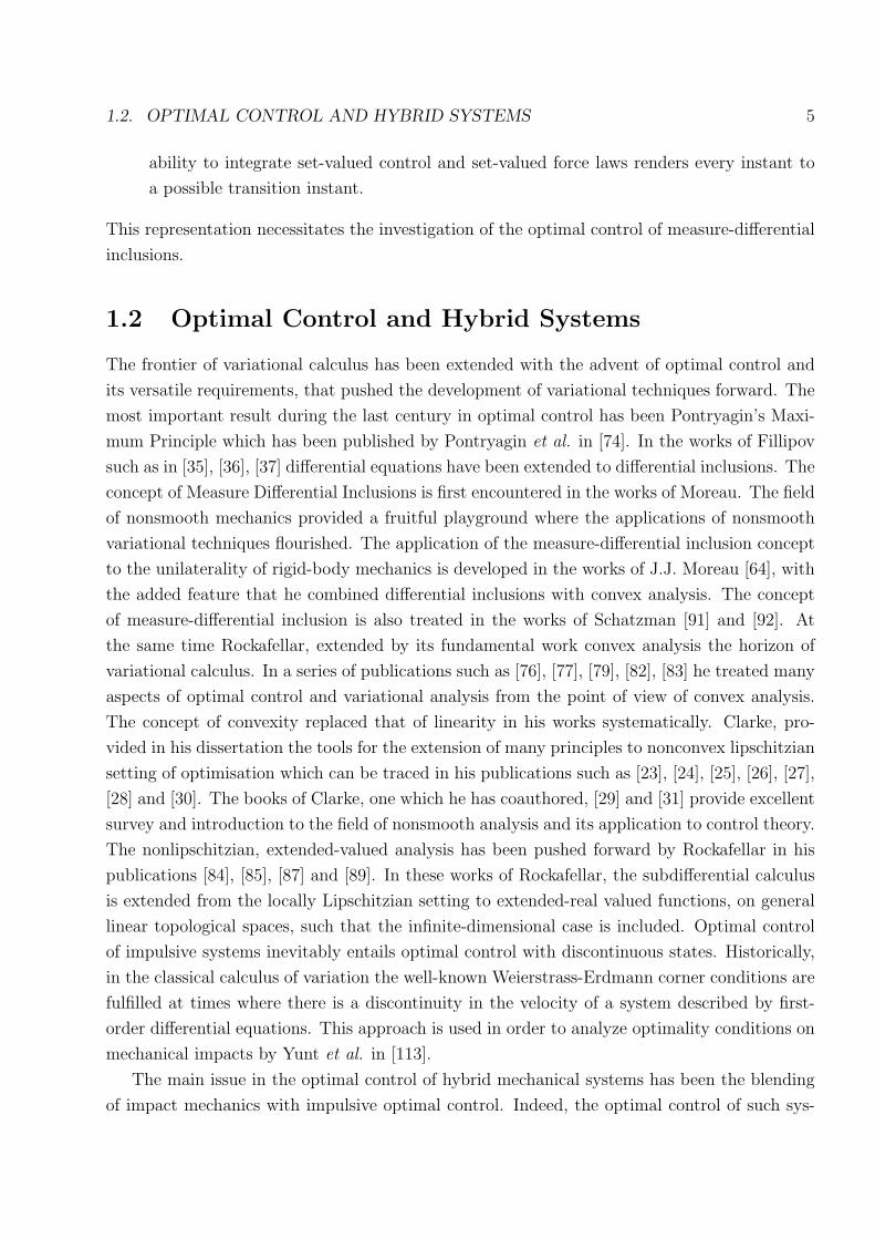
1.2. OPTIMAL CONTROL AND HYBRID SYSTEMS 5
ability to integrate set-valued control and set-valued force laws renders every instant to
a possible transition instant.
This representation necessitates the investigation of the optimal control of measure-differential
inclusions.
1.2 Optimal Control and Hybrid Systems
The frontier of variational calculus has been extended with the advent of optimal control and
its versatile requirements, that pushed the development of variational techniques forward. The
most important result during the last century in optimal control has been Pontryagin’s Maxi-
mum Principle which has been published by Pontryagin et al. in [74]. In the works of Fillipov
such as in [35], [36], [37] differential equations have been extended to differential inclusions. The
concept of Measure Differential Inclusions is first encountered in the works of Moreau. The field
of nonsmooth mechanics provided a fruitful playground where the applications of nonsmooth
variational techniques flourished. The application of the measure-differential inclusion concept
to the unilaterality of rigid-body mechanics is developed in the works of J.J. Moreau [64], with
the added feature that he combined differential inclusions with convex analysis. The concept
of measure-differential inclusion is also treated in the works of Schatzman [91] and [92]. At
the same time Rockafellar, extended by its fundamental work convex analysis the horizon of
variational calculus. In a series of publications such as [76], [77], [79], [82], [83] he treated many
aspects of optimal control and variational analysis from the point of view of convex analysis.
The concept of convexity replaced that of linearity in his works systematically. Clarke, pro-
vided in his dissertation the tools for the extension of many principles to nonconvex lipschitzian
setting of optimisation which can be traced in his publications such as [23], [24], [25], [26], [27],
[28] and [30]. The books of Clarke, one which he has coauthored, [29] and [31] provide excellent
survey and introduction to the field of nonsmooth analysis and its application to control theory.
The nonlipschitzian, extended-valued analysis has been pushed forward by Rockafellar in his
publications [84], [85], [87] and [89]. In these works of Rockafellar, the subdifferential calculus
is extended from the locally Lipschitzian setting to extended-real valued functions, on general
linear topological spaces, such that the infinite-dimensional case is included. Optimal control
of impulsive systems inevitably entails optimal control with discontinuous states. Historically,
in the classical calculus of variation the well-known Weierstrass-Erdmann corner conditions are
fulfilled at times where there is a discontinuity in the velocity of a system described by first-
order differential equations. This approach is used in order to analyze optimality conditions on
mechanical impacts by Yunt et al. in [113].
The main issue in the optimal control of hybrid mechanical systems has been the blending
of impact mechanics with impulsive optimal control. Indeed, the optimal control of such sys-

6 CHAPTER 1. INTRODUCTION
tems entails unavoidably impulsive control. In what follows next, the new concepts required
to deal with this specific problem are introduced shortly. First of all a new concept of partial
integration of differential measures is required. In the framework of integration theory, this has
long been recognised as a problem if state and costate should become concurrently discontinu-
ous as has been addressed by Moreau [64] and Rockafellar [76]. Rockafellar studied in [76] the
discontinuity of the dual state in constrained convex optimal control problems but dispensed
of attacking the problem of concurrent discontinuity of state and costate. Moreau gave in [64]
partial integration formulas for differential measures in general bilinear forms. In [68] Murray
studies the extension and existence theorems of problems in calculus of variation to the setting
when impulsive controls are applied and state discontinuity occurs. He bases his work on [76],
and outlines in his motivation that jumps in the states may occur due to constraints on the
dual dynamics which are reached by the costate, as economics as a field of application in mind.
In [18] Bressan studies several classes of impulsive Lagrangian systems. The main focus is
impulses generated by sudden parameter changes such as inertial parameters that affect the
momentum balance, or impulses arising due to structure of constraints of a mechanical system.
A certain class of impulsive systems that resemble discontinuous diffusion processes are treated
in [12] by Bensoussan. In [112] by Yunt, the concept of internal boundary variations are in-
troduced, from the point of view that the instant of state discontinuity constitute an internal
boundary in the optimal control problem. The necessity that at a location of transition several
conditions have to be fulfilled, gives rise to the idea of some sort of transversality conditions if
one begins to consider an instant of discontinuity as a two-sided boundary where to arcs are
”joined” discontinuously. So the concepts of internal boundary variations and discontinuous
transversality conditions are given birth to, which are twins in some sense. They subsume the
classical boundary variations and transversality conditions naturally, since the classical ones
constitute the unilateral versions of bilateral new concepts. A fundamental difference in vari-
ous approaches in modeling of state discontinuity is the character of the interval on which the
discontinuity and the impulsive control action acts on the system. A common approach is to
assume that the discontinuity happens on a Lebesgue negligible interval whereas in the other
approach the interval of discontinuity is opened and a transition dynamics is implanted. In
the realm of impulsive optimal control, both approaches are represented. There are a wide
variety of articles devoted to the analysis of the impact phase in the optimal impulsive control,
where the ”contact stiffness” is taken very high, such that a rigid-body behaviour is attained
in the limit. In the references by Galyaev [41], Bentsman et al. [60] and the book by Miller
[59] the discontinuous time change approach is the underlying technique. By using the special
transformation of the time scale, the method enables the conversion of an impulsive optimal
control problem to standard one with ordinary differential equations, which is formulated for
some auxiliary system described by ordinary differential equations with bounded controls. Re-

1.2. OPTIMAL CONTROL AND HYBRID SYSTEMS 7
cently, Bentsman and Miller et al. and Miller and Bentsman, further complicated the analysis
by considering the dynamics that may be induced through the interaction with the control
strategy such as impulsive sliding modes and zeno systems, and propose it as an alternative
approach to the complementarity approach in [13] and [58]. In [67] by Murphey some aspects
of nonsmooth dynamics of mechanical systems and control aspects are treated. There Murphey
introduces the terminology multiple-model systems, referring to the fact that through contact
interactions such as stick-slip transitions, the mechanical system can be represented by differ-
ent differential equations depending on the state of the contacts. His approach falls generally
into the approach of discrete-event system analysis in hybrid system terminology. The tran-
sitions between the models are on a set of measure zero. The author focuses on the stability
analysis of systems with friction transitions. In the approaches provided in references such as
[8], [48] and [96], the impulsive control problem is transformed into a problem of an ordinary
differential inclusion problem, which requires to determine trajectories for the ”discontinuous”
states during the ”impulsive” control action. Though the modeling approach depends on the
task, this approach has two main disadvantages. Hybrid system theory is based mainly on the
assumption that the transitions happen instantaneously, and the main modeling approaches are
based on the instantaneous transition concept. The second disadvantage lies in the inability of
this interval opening approach to tackle with the combinatorial nature of the mode sequencing
and transition time and location determination problem. Philosophically, in order to resolve
this combinatorial problem properly every instant must be equipped with ability to have the
potential to switch to all other possible modes, which is practically not possible in the interval
opening approach. In [60], impulses arising from unilateral constraints are considered but again
in the framework of interval-opening approach and transformation technique. The instanta-
neous transition approach is in comparison to other impulsive necessary conditions consistent
with different common hybrid system modeling methods in which transitions happen instan-
taneously such as in [17]. In [40] Galbraith and Vinter discuss the optimal control of hybrid
systems with an infinite set of discrete states in an abstract setting. An event driven approach
to hybrid dynamical systems is used similar to [17]. The properties of the resulting value func-
tion is characterised. The authors claim that the analysis is extendable to optimal control of
dynamical systems with discontinuous states by invoking bounds on the transition instants.
Egerstedt et al. discuss in [33] and [34] a numerical algorithm based on the calculation of the
gradient of the value function with respect to switching times and propose a gradient descent
based algorithm that determines suboptimal solutions and the method is for continuous state
trajectories which are Lipschitz. In [102] Verriest et al. consider an impulsive optimal control
problem with discontinuity in the system state and delay response to impulsive input. Neces-
sary conditions are stated in first-order form by making use of the Hamiltonian concept. The
instant of impulsive control action and transition locations are free, however, the variations at

8 CHAPTER 1. INTRODUCTION
the internal boundaries of the time domain where the system state is discontinuous seemingly
only derived by the assumption that the variations of the pre-, and post-transition states are
having only the component for fixed impulse time, which seems contradictive to the proposed
problem. In two publications [106] and [107] Xu and Antsaklis present a direct numerical
method for the switching time optimisation for systems without state discontinuity at transi-
tions. Shaikh presents in [93] and [94] necessary and sufficient conditions for hybrid dynamical
systems with state-continuous transitions by making use of needle variation technique. In [104]
considers the optimal control of impulsive dynamical systems, which are exposed at fixed time-
instants to impulses that are generated autonomously. The magnitude of the impulsive force
is dependent on the system state but the controls are ordinary and nonimpulsive. In a series
of publications Ahmed [2], [3], [4] and [5] studies existence and necessary conditions for the
optimal control of measure-differential equations of the form:
dx = Ax dt + f(x) dt + g(x) ν(dt), x(0) = ξ, t ≥ 0. (1.1)
He discusses the existence and regularity of the solutions and relates them to optimal control.
There are some works devoted to the complementarity modeling and optimal control of mechan-
ical systems as given in references [109], [114], [115], [116]. In [20] Brogliato studies the problem
of quadratic optimal control of unilaterally constrained linear time-invariant systems. His mo-
tivation is to define a class of optimal control problems for which the higher-order Moreau’s
sweeping process constitutes the numerical resolution of its necessary conditions. Optimal con-
trol of mechanical systems with unilateral constraints has been analysed case dependent in
several publications, such as in [108], where an optimal control strategy for the high jump of
an hopper is studied based on complementarity modeling.
In this work, it is assumed that the instant of discontinuity is reduced to an instant with
Lebesgue measure zero, instead of taking an interval opening approach, which is the approach
considered in literature so far.
1.3 Internal Boundary Variations and
Discontinuous Transversality Conditions
The approach taken in this thesis, before being converted into variational necessary conditions,
is first expounded in its philosophical approach. A transition with a discontinuity in the state
can be regarded as an internal boundary in the domain of interest. Historically, the Weierstrass-
Erdmann corner conditions were among the first variational conditions to deal with trajectories
with a corner. The idea of internal boundary variations and discontinuous transversality condi-
tions emanated from the motivation to provide variational criteria for time and location, at the
instants where impulsive transitions happen under constraints and discontinuity in the state.

1.3. DISCONTINUOUS TRANSVERSALITY CONDITIONS 9
An early attempt of the author is given in [113] where under relatively restrictive assumptions
and using Weierstrass-Erdmann corner conditions optimality conditions for mechanical impacts
are investigated.
A time instant of Lebesgue measure zero is considered as a transition time ti ∈ IT if one of
the two events occur together or for itself:
• Event 1 Some directions of motion of the system are opened or closed by the control
strategy, which entails a change in the degrees of freedom (DOF) of the system.
• Event 2 An impulsive control action is exerted on the system, which may be accompanied
by a discontinuity of the generalised velocities of the Lagrangian system.
Here IT denotes the set of transition instants of the process.
The concurrence of both events where some directions of motion are closed is called ”block-
ing”. In the time-optimal control of dynamical systems one has to consider the variations in
the end time. In the classical calculus of variations where the final state and final time are
free, the variations of the final state are composed of two parts, namely, the part that arises of
the variations at a given time and the part arising from variations due to final time. Since the
transitions times are assumed to be free, the two-part character of the variations at pre-, and
post-transition states is considered. The assumptions during a possibly impactive transition
are given as follows:
• The transitions may be impactively.
• The generalised position remain unchanged during transition.
• The impulsive control action acts on the system at a time instants ti which are Lebesgue-
negligible and are countably many.
• At a possibly impactive transition, the pre-transition controller configuration is assumed
to be effective.
• There are no transitions at initial time t0 and final time tf .
The assumption that impulsive forces are Dirac distributions, enable their consideration on an
atomic instant of time, since the integral of the Dirac distribution is constant, irrespective of the
measure of its support. The above stated assumptions are converted into requirements to the
variations at the internal boundaries. At the boundaries of the time domain, the pre-transition
state variations are considered separately from the post-transition variations. In impact me-
chanics, the generalised accelerations and velocities are eligible to become discontinuous where
as the generalised positions are of absolutely continuous character. The absolute continuity
of the generalised positions means that the total variation of the generalised positions at the

10 CHAPTER 1. INTRODUCTION
pre-transition and post-transition instants are equal. The pre-transition and post-transition
variations are interrelated by the transition conditions which can be seen as the fundaments of
transversality conditions that join two trajectories discontinuously. The transition conditions
are introduced symmetrically with respect to pre-, and post-transition states. The transition
conditions are of two types, namely, the impact equations and the constitutive impact laws.
The impact equations relate the discontinuity in the impulse of the Lagrangian system to the
impulsive forces/controls. The impact law (.i.e. the moreau-newton impact law), however, is
a constitutive law which is chosen depending on the modeling approach preferred. As a case
study, in reference [115] by Yunt the blocking of some DOF of an underactuated manipulator
by tangential fully-inelastic impact is discussed and the necessary conditions are stated.
1.4 Numerical Analysis
The literature on the numerical techniques that have found application in the trajectory opti-
misation and optimal control of dynamical systems is vast. The numerical methods in optimal
control are divided in two broad classes, namely, direct methods and indirect methods. The
direct methods comprise numerical approaches where after a suitable discretisation method for
the dynamics the goal function is minimised directly. These methods use only control and
state variables as optimisation variables and dispense completely with adjoint variables. The
discretised adjoint states are obtained by a post-optimal calculation using the dual multipliers
of the resulting nonlinear programming problem. In indirect methods one has also the nec-
essary conditions which have to be fulfilled. The references [15] by Betts and [22] Buskens et
al. provide a general overview on the methods that have been used so far if dynamical pro-
cesses are modeled as differential equations with constraints among many others. The theory of
necessary conditions for optimal control problems with control and state constraints has been
developed in the second part of the last decade. The theory at hand treats optimal solutions as
solutions of multi-point boundary value problems (MBVP). For this class of MBVP’s, shooting
techniques have been developed as efficient and reliable numerical methods providing highly
accurate solutions. However, these methods need a close enough initial guess of the optimal
state, control and adjoint variables and require a detailed a priori knowledge of the structure of
the optimal solution, such as the number of active time intervals for each of the constraints. In
practice, it is difficult to determine the structure of the optimal control and to find appropriate
estimates for the adjoint variables a priori.
When considered from the perspective of discretisation, there are two major approaches to
handle the optimal control of finite-dimensional Lagrangian systems in the trajectory optimi-
sation numerically. These are based on time-stepping (sweeping) and event-driven approaches.
Event-driven approaches lead to optimisation problems that belong to the class of mixed integer

1.4. NUMERICAL ANALYSIS 11
programming problems and branch and bound techniques are methods used in order to search
for the minimum. In this thesis, however, the time-stepping approach is considered, which is
the natural numerical extension of the MDI representation of the dynamics.
Numerically, the treatment of the optimal control of FDLS is related to the applied math-
ematics branch called Mathematical Programming of Equilibrium Constraints. In literature
there are numerous methods for trajectory optimisation of hybrid dynamical systems. In the
framework of this thesis, they are investigated in two broad classes, namely, switching finite-
dimensional Lagrangian systems and hybrid finite-dimensional Lagrangian systems. In [73] by
Outrata et al. a MPEC is defined as an optimisation problem in which the essential constraints
are defined by parametric variational inequality or complementarity systems. One of the many
representations of a MPEC can be stated as follows:
minx,z
f(x, z), (1.2)
z ∈ S(x), (1.3)
x ∈ Uad, z ∈ Z. (1.4)
The problem described by (1.2), (1.3) and (1.4) includes a subclass of so-called bilevel programs,
where S assigns each x ∈ Uad the necessary conditions of a ”lower-level” optimisation problem.
In the case where the complementarity system arises from mechanical systems without Coulomb
friction, a so-called subclass of MPEC, namely, bilevel programs apply. In references [32] by
Cottle et al. and [70] by Murty, detailed treatment of complementarities and optimisation can
be found. References [57] by Luo et al. and [73] by Outrata treat MPEC and bilevel programs
extensively. In the framework of this thesis, the control action is represented by x ∈ Uad. The
differential measures of control can be considered as the variables of the ”higher-level” opti-
misation problem whereas the contact forces and states are the variables of the ”lower-level”
problem. By analogy, the measure-differential inclusion, that describes the dynamics as a bal-
ance of measures, can be considered as the necessary conditions of a ”lower-level” optimisation
problem represented by the saddle-region restraining set S. The comprehension of the struc-
ture of structure-variant mechanical systems paves the way to suitable numerical algorithms, by
considering of this unique nature of mechanical systems reveals through the extended principle
of Gauss the necessary optimality conditions in complementarity and proximal form for FDLS.
In [63] it has been shown that the determination of the accelerations of a mechanical system
subject to unilateral constraints without friction can be cast into a primal and dual quadratic
programming problem. Further, it is shown that a generalisation of the Gauss’ variational
principle is valid in the case of unilateral constraints without friction. In [44], it is shown that a
quadratic programming problem can be obtained if Tresca type friction, for which the normal
force is decoupled from the tangential force, exists and that the equations of motion along with
the linear-complementarity conditions constitute necessary Karush-Kuhn-Tucker conditions of

12 CHAPTER 1. INTRODUCTION
optimality for the quadratic programming problem. If Coulomb type friction exists at the con-
tacts, then the optimal control problem is subject to variational inequalities (VI) and there
does not exist a QP of which solution is equivalently representable by the resulting VI.
There are several historical corner stones in the numerical analysis of complementarity
systems. The study of complementarity problems is a flourishing field since its advent at
the beginning of the sixties. In the beginning, the linear complementarity problem drew the
attention because of the structure of the Karush-Kuhn Tucker conditions of a general Quadratic
Programming (QP) Problem, which has a LCP structure. The formulation of the computation
of the Nash equilibrium point of a bimatrix game as a LCP by Howson and Lemke developed
an efficient pivoting algorithm, the complementary pivot method, marked the establishment of
the LCP’s as a branch of applied mathematics of its own. In 1968, came the unification of linear
and quadratic programming problems and bimatrix games in the LCP framework by Cottle
and Dantzig. The nonlinear complementarity problem (NCP) has been introduced by Cottle
in his doctor of philosophy thesis in 1964. The concept of Variational Inequality Problem has
been defined in 1966 by Hartman and Stampacchia in the framework to compute stationary
points of nonlinear programs.
The numerical optimisation in this thesis for hybrid Lagrangian trajectories rely on the
augmented Lagrangian method which has been extensively investigated by R. T. Rockafellar
in his works such in [80], [81] and [86]. There are several aspects that make the augmented
Lagrangian approach favorable in comparison to other approaches. In exact penalty methods,
instead of performing a sequence of minimisations, a single minimisation is performed but the
penalty parameter has to be set very high, such that ill-conditioning is caused, and depending
on the minimisation method used the condition number of the Hessian matrix is severed. The
sequential minimisation besides preventing ill-conditioning, allows partial minimisations espe-
cially at the initial stages of the successive minimisations such that the successive minimisations
proceed faster then expected. The global optimizing property as in the exact penalty approach
is preserved. The Newton method in the minimisation of unconstrained functions is a favored
method because of its superlinear convergence in the vicinity of the solution. However, in large
scale optimisation problems where the structure of the Hessian matrix is not sparse, the eval-
uation of the Hessian matrix becomes cumbersome. In the case of the augmented Lagrangian
technique, in general, by the convexification induced by adding quadratic penalty terms to the
goal function, the structure of the Hessian matrix becomes dense. In such cases, quasi-Newton
methods are used in order to extrapolate the Hessian matrix by a formula like BFGS method.
If the function to be minimised is nonsmooth, then the nonuniqueness and unboundedness
of the Hessian may cause problems. A way to circumvent the problem of the nonuniqueness
and unboundedness of the Hessian matrix often induced by using reformulation functions is to
use smoothing. This has the disadvantage however that the smoothing parameter has to be

1.4. NUMERICAL ANALYSIS 13
adjusted in the course of the optimisation, which reduces the speed of the algorithm as well.
The modified conjugate gradient methods offer a trade-off by performing a minimisation based
on second-order information without calculating them. The only required information is first-
order information such as an element of the subgradient and second-order information such as
estimates of the Hessian are extrapolated numerically, and it is not necessary to calculate the
dense Hessian matrix.
The concept of controlling hybrid systems requires to make decision of discrete decisions.
The dependence of the optimisation problem to decisions is treated in the framework of sen-
sitivity analysis. As can be expected, the sensitivity of a numerical treatment of an optimal
control problem to discrete decisions is high. In order to accomplish the sensitivity analysis
the value function is discussed in the nonsmooth setting and is related to the augmented La-
grangian approach. Lagrange multipliers are the measure for the sensitivity of an optimisation
problem to a given set of constraints. Classically, Lagrange multipliers were viewed as auxiliary
variables, which were introduced in a constrained minimisation problem in order to write first-
order optimality conditions as a system of equations. The needs arising from more complicated
constraint structures required an in-depth understanding of dual variables, and they have been
characterised by the methods of nonsmooth geometry, which makes use of one-sided tangent
and normal vectors to a set of points that satisfy the constraints. The modern approach to
Lagrange multipliers is presented in [27] and [90].
The classical theory of optimisation presumes certain differentiability and strong regularity
assumptions. However, these assumptions are too demanding for many practical applications,
since functions involved are often nonsmooth, that is, they are not necessarily differentiable.
The source of the nonsmoothness may be the objective function itself, its possible interior
function, or both. Moreover, there exists so-called stiff problems that are analytically smooth
but numerically nonsmooth. This means that the gradient varies too rapidly, and, thus, these
problems behave like nonsmooth problems. The methods for nonsmooth optimisation can
be divided into two main classes, namely, subgradient methods and bundle methods. Both
approaches are based on the assumption that functionals to be minimised are locally Lipschitz
continuous. This assumption is necessary because of the requirement to evaluate the functional
and one of its arbitrary subgradients in every point of the domain of interest. The problem, thus,
need not to be differentiable or convex. The subgradient methods have mainly developed in the
60s in the Soviet Union and an excellent overview is given in [95]. Their basic idea is to generalize
the methods for smooth problems by replacing the gradient by an arbitrary subgradient. The
main handicap for these methods is the absence of an implementable stopping criterion. The
fact that the direction opposite to an arbitrary subgradient need not yield a direction of descent,
excludes them from the class of descent methods. The second class of methods are the bundle
methods. The main idea is to exploit the previous iterations by gathering the subgradient

14 CHAPTER 1. INTRODUCTION
information into a bundle. The first bundle method, the so-called ε-steepest descent method
was developed in Lemarechal in [54]. It was based on the conjugate subgradient method by
Lemarechal [53] and Wolfe [105]. In [49] Kiwiel gave a new approach to bundle methods,
which was based on the classical cutting plane method. The main idea in this method is to
form a convex piecewise linear approximation to the objective function using the linearisations
generated by the subgradients.
The thesis is structured as follows:
Chapter 1 provides an introduction to this work. In this chapter the reasons, why this
problem is attacked, is presented. Further, it shall give the reader an overview on the character
of problem being handled. It also provides historical background of vast areas of research such
as calculus of variations and optimal control, measure theory, set-valued analysis, nonsmooth
analysis, variational inequalities and complementarities, hybrid system computation and control
on a rather limited space with emphasis on key issues, persons and events. This shall enable
the placement of this work in a proper place in a long research history. In the introduction
in a comparative manner, the differences to other works done in this field is provided. These
comparisons include approaches in numerical issues as well as theoretical considerations.
Chapter 2 deals with the fundamental issue of modeling impulsively controlled FDLS. The
modeling is a fundamental attribute that shapes the optimisation approach extensively. The
chapter begins with the analysis of projected Newton-Euler Equations in impulsive control
form which is first presented in [110]. In this context the concept of set-valued, impulsive and
unbounded controls is introduced. A measure-differential inclusion (MDI) based modeling ap-
proach for finite-dimensional Lagrangian systems is introduced, that can exhibit autonomous or
controlled mode transitions, accompanied by discontinuities on velocity and acceleration level.
The introduced framework has the ability to model and control hybrid mechanical systems with
discontinuous transitions among different system modes. Modeling of FDLS as Linear Comple-
mentarity Problem (LCP) is presented. The definition of hybrid finite-dimensional Lagrangian
system is given in association with this modeling approach. A general measure-differential
inclusion representation of finite-dimensional Lagrangian systems is derived, in which the set-
valued inclusions are represented as linear complementarities. The aim is to extend the existing
modeling framework such that controls of impulsive and set-valued character are fit in. Start-
ing from the Lagrangian formalism in impulsive control form, the modeling is further detailed
in the successive section to include a linear complementarity structure, that enables to con-
sider the interaction of impulsive controls with together with set-valued impulsive interactions
of the system with the surroundings. The Lagrangian formalism in impulsive control form is
already discussed in [110]. The main part of the complementarity modeling of controlled com-
plementarity mechanical system is published in [117]. The model in chapter 2 about modeling
complementarity systems is enriched by fitting in properly the measure theory, and extending

1.4. NUMERICAL ANALYSIS 15
the modeling on acceleration level, on impactive form and measure-differential inclusion form
to some suitable quadratic problems which can be seen as variants of the extended problem
of Gauss and its dual, which first has been discussed in framework of QP by [63] for rigid
body mechanical systems of which dynamics are represented by differential equations subject
to constraints on position level. The existence of such quadratic programs in different cases is
in the opinion of the author important for numerical considerations. The idea to consider such
variants of the extended problem of Gauss and its dual is first mentioned in [115]. Further in
[115], the complementarity representation of blocking is used, for which a detailed discussion
and derivation is provided in chapter two. The chapter concludes with a case study, in which
the modeling framework for underactuated scleronomic mechanical systems with impactively
blockable DOF is presented. This modeling framework is already discussed in [111], and is
supplemented here further by the analysis of dissipated energy, change of kinetic energy and of
the impulse of the system.
Chapter 3 is devoted to the numerical methods in calculating optimal trajectories. There are
two numerical methods that are being introduced in this chapter, one nonlinear programming
approach and a shooting method. Both methods reside on augmented Lagrangian techniques,
because of its efficiency in tackling with nonconvex optimisation problems. After introducing
the preliminaries of nonsmooth analysis and differentiation in finite-dimensional spaces, the
local and global properties of the augmented Lagrangian method is discussed. The properties
of the augmented Lagrangian method are analysed by making use of the techniques that derive
from nonsmooth geometrical considerations. The introduced methods are direct methods. Two
mechanical models are investigated in detail. In the NLP case the global optimal trajectories
of an underactuated double pendulum with impulsively blockable DOF is presented. In the
analysis of the shooting method, a five-DOF differential drive model is used to present the
properties of the shooting method.
Chapter 4 deals with the derivation of necessary conditions for the impulsive optimal con-
trol problem in second-order form, since dynamic mechanical systems have a representation in
second-order differential form. The main result of this chapter is published in [112]. In this chap-
ter the discontinuous transversality conditions and internal boundary variations are expounded
in detail. Necessary conditions for the impulsive time-optimal control of finite-dimensional
Lagrangian systems is stated. The derivation is based on the application of subdifferential
calculus techniques, to lower-semicontinuous extended-valued functionals. The necessary con-
ditions for the impulsive time-optimal control of underactuated manipulators with impulsively
blockable DOF is provided. The concepts of internal boundary variations and discontinuous
transversality conditions are introduced in detail in this chapter.
Chapter 5 is devoted to the derivation of the same necessary conditions as in Chapter 4
in the first-order form, which gives access to the well-known Hamiltonian framework. The

16 CHAPTER 1. INTRODUCTION
subdifferential calculus for extended-real valued functions, on general linear topological spaces
as developed by Rockafellar is the main instrumentation in the derivation of the necessary
conditions. Further, a hybrid system definition of finite-dimensional Lagrangian systems is
given, and a hybrid impulsive minimum principle is stated. The necessary conditions for the
time-optimal control of underactuated manipulators with blockable DOF is stated in a first-
order system setting. The main of the results are already published and presented in [110].
Necessary conditions are stated in the first-order form, and by considering upper directional
derivatives of the Hamiltonian in different phases of motion, the structure of the dual state is
characterised.
Chapter 6 concludes with a discussion of the results and future directions of work. The
contributions of the PhD Thesis can be summarised in several points:
Claims of Originality
• Establishment of the relationship between finite-dimensional Lagrangian systems (FDLS)
and Hybrid System Modeling and Control within the Measure Differential Inclusion frame-
work
• The definition and introduction of internal boundary variations and discontinuous transver-
sality conditions as generalisations to their classical counterparts
• The relation of the Discontinuous Transversality Conditions to impulsive optimal control
• Proposition of a NLP algorithm and shooting method for the analysis of Hybrid La-
grangian systems based on Moreau’s sweeping process
• Complementarity characterisation of blocking as a set-valued control law
• Statement of Necessary Impulsive Optimal Control Conditions for structure-variant finite-
dimensional Lagrangian systems in Second-Order Form
• Statement of Necessary Impulsive Optimal Control Conditions for structure-variant finite-
dimensional Lagrangian systems in First-Order Form
• Application of the derived concepts to the control of underactuated manipulators with
impulsively blockable DOF
• The general development of a modeling framework for the impulsive control of hybrid
finite-dimensional Lagrangian systems
• The introduction and development of a single-shooting method for switched Lagrangian
systems based on the augmented Lagrangian method and time-stepping integration.

1.4. NUMERICAL ANALYSIS 17
• The introduction and development of a direct method that is based on an augmented La-
grangian based nonlinear programming scheme for the determination optimal trajectories
of finite-dimensional impulsive hybrid Lagrangian systems.
• The development of an augmented Lagrangian based MPEC optimisation scheme that
performs the minimisation based on modified conjugate gradients methods.
• The combinatorial NP-hard nature of mixed-integer programming approaches is circum-
vented and a polynomial time methods is developed that is able to choose a sequence of
transitions and modes.
This work is based on following publications:
Published and Submitted Publications
• K. Yunt and Ch. Glocker, Trajectory Optimisation of Hybrid Mechanical Systems using
SUMT, IEEE Proc. of Advanced Motion Control, Istanbul, 2006, pp 665-671.
• K. Yunt and Ch. Glocker, Time-Optimal Trajectories of a Differential-Drive Robot,
Proceedings of the Fifth Euromech Nonlinear Dynamics Conference, D. H. Van Campen,
M. D. Lazurko, W.P.J.M van der Oever (Eds), pp. 1589-1596.
• K. Yunt and Ch. Glocker, A Combined Continuation and Penalty Method for the Deter-
mination of Optimal Hybrid Mechanical Trajectories, IUTAM Symposium on Dynamics
and Control of Nonlinear Systems with Uncertainty 2006, H.Y. Yu and E.Kreuzer (Eds.),
IUTAM Bookseries, Springer, 2007, pp. 187-196.
• K. Yunt, Optimal Trajectory Planning for Structure-Variant Mechanical Systems, IEEE
Proc. of Int. Workshop on Variable Structure Systems VSS’06, 2006, pp 298-303.
• K. Yunt and Ch. Glocker, Modeling and Optimal Control of Hybrid Rigid-Body Me-
chanical Systems, Hybrid System Computation and Control (HSCC07), A. Bemporad, A.
Bichi and G. Buttazzo (eds.), Springer, Lecture Notes in Computer Science (LNCS) 4416,
2007, pp 614-627.
• K. Yunt, Impulsive Time-Optimal Control of Underactuated Manipulators with Im-
pactively Blockable Degrees of Freedom, European Control Conference (ECC’07), 2007,
pp 3977-3984.
• K. Yunt, Impulsive Time-Optimal Control of Structure-Variant Rigid-Body Mechanical
Systems, 3rd International IEEE Scientific Conference on Physics and Control (Physcon
2007), 2007 IPACS Open Library ://lib.physcon.ru.

18 CHAPTER 1. INTRODUCTION
• K. Yunt, Necessary Conditions for Impulsive time-optimal Control of Finite-Dimensional
Lagrangian Systems, Hybrid System Computation and Control (HSCC08), M. Egerstedt
and B. Mishra (eds.), Springer, Lecture Notes in Computer Science (LNCS), pp. 556-569.
• K. Yunt and Ch. Glocker, Optimality Conditions for Mechanical Impacts, Proceedings of
Applied Mathematics and Mechanics , GAMM 2004, Vol.4, pp. 630-631.
• K. Yunt, Necessary Conditions for the Impulsive Optimal Control of Multibody Me-
chanical Systems, Zeitschrift fur Angewandte Mathematik und Mechanik , (submitted on
March, 15th 2008)
• K. Yunt, Necessary Conditions for the Impulsive Time-Optimal Control of Rigid-Body
Lagrangian Systems, Systems and Control Letters, (submitted on September, 24th 2007)

Chapter 2
Modeling of Hybrid Finite-Dimensional
Lagrangian Systems
2.1 Preliminaries
All the vectors are considered as column vectors and, correspondingly, all the transposed vectors
are considered as row vectors. The usual inner product is denoted by 〈x, y 〉 and ‖x‖ represents
the Euclidean norm.
〈x, y 〉 =n∑
i=1
xi yi (2.1)
‖x‖ = 〈x, x〉 12 (2.2)
where x and y are in Rn and xi, yi ∈ R are the ith components of the relating vectors.
Definition 2.1.1 -Indicator Function The indicator function ΨC(x) of a convex set Ctakes the value zero if x ∈ C and infinity otherwise,
ΨC(x) =
0 if x ∈ C∞ if x /∈ C. (2.3)
Definition 2.1.2 -Conjugate Function The conjugate function f ∗(x∗) of a convex func-
tion f(x) is defined as:
f ∗(x∗) = supx
(〈x, x∗〉 − f(x)) . (2.4)
Definition 2.1.3 -Subdifferential of a Convex Function The subdifferential ∂ f(x) of
a convex function f(x) is a set containing the gradients of all supporting hyperplanes of f(x),
∂ f(x) = y | f(x∗) ≥ f(x) + 〈y, x− x〉 ; ∀x∗ . (2.5)
Definition 2.1.4 -Normal Cone The normal cone NC(x) to a convex set C is the set of
all vectors that have an obtuse angle with all vectors x emanating from C to any x ∈ C,
NC = y | 〈y, x− x〉 ≤ 0; ∀x ∈ C; ∀x ∈ C . (2.6)
19

20 CHAPTER 2. MODELING OF HYBRID FDLS
The normal cone to a convex set C at the point x ∈ C is given by NC(x) in the sense of convex
analysis [82].
Definition 2.1.5 -The Linear Complementarity Problem [70] Given A ∈ Rn×n, b ∈Rn find w = (wj) ∈ Rn, z = (zj) ∈ Rn satisfying
w −Az = b; w, z º 0; 〈w, z〉 = 0. (2.7)
This LCP is denoted by the tuple (b, A).
Lemma 2.1.1 The subdifferential of the indicator function is the inverse of the subdiffer-
ential of the support function,
x∗ ∈ ∂ΨC(x) ⇔ x ∈ ∂Ψ∗C(x
∗). (2.8)
Lemma 2.1.2 The basic complementarity relation
x ≥ 0, y ≥ 0, x y = 0, (2.9)
can equivalently represented as:
x ∈ NR+0(y) (2.10)
or
y ∈ N ∗R+
0(x). (2.11)
Lemma 2.1.3 The set-valued Signum relation y ∈ Sgn(x)
y =
1 if x∈ R+,
[-1,1] if x=0,
-1 if x∈ R−.
(2.12)
can be decomposed into two UPR relations:
yL ∈ Upr(xL)− 1 (2.13)
yR ∈ −Upr(xR) + 1 (2.14)
where
y = yL + yR, x = xR − xL. (2.15)
The generalisation of the fundamental LCP is the mixed LCP (mLCP).
Definition 2.1.6 -The Mixed Linear Complementarity Problem [70] Given A ∈Rn×n, B ∈ Rm×m,C ∈ Rn×m, D ∈ Rm×n, a ∈ Rn, b ∈ Rm, find v ∈ Rm,u ∈ Rn satisfying
a + Au + Cv = 0, b + Du + Bv ≥ 0, v ≥ 0, 〈v,b + Du + Bv〉 = 0. (2.16)

2.1. PRELIMINARIES 21
Upr( )
y
x
xy =
Figure 2.1: Unilateral primitive.
Sgn( ) Upr( ) Upr( )+x
x
y
1
1 1
1
xL
xR
xL 1 1x
R
yL
yR
Figure 2.2: Decomposition of the Signum relation into two Uprs.

22 CHAPTER 2. MODELING OF HYBRID FDLS
The right-continuous and left-continuous regularisations of a function f , which is a mapping
of I to a Hausdorff topological space E ; becomes important if one considers that for every ti ∈ IT
the right-side limit given by:
f+(ti) = lims→ti, s>t
f(s) (2.17)
may differ from f(ti), if it exists. Symmetrically, the left-side limit, if it exists, is denoted by
f−(ti). Following proposition is used often in this work:
Proposition 2.1.1 [64] Let E be regular and let f : I → E be such that for every t ∈ Idifferent from the possible right end of I, there exists f+(t) ; then
f+(t) = lims→t, s>t
f+(s). (2.18)
If, in addition, for every t different from the possible left end of I, there exists ; then
f−(t) = lims→t, s>t
f+(s). (2.19)
As short hand notation one has:
(f+)+ = f+, (f−)+ = f+, (f−)− = f−, (f+)− = f−. (2.20)
Properties of Bounded Variaton Functions Every function of bounded variation u, in
this case the generalised velocities of the mechanical system, is associated with an Rn-valued
regular Borel measure du on [t0, t1]. The atoms for du occur only at discontinuities of u, of
which there are at most countably many. Trajectories of bounded variation in Rn are defined
to be an equivalence class, and the space of all arcs is denoted by BV . The space of absolutely
continuous arcs AC is a subspace of BV . There are uniquely determined functions u+(t) and
u−(t) in [t0, t1] → Rn, right and left continuous respectively, such that u+(t) = u−(t) = u(t)
at all the nonatomic points, and at the end points u−(t0) = u(t0) and u+(tf) = u(tf) are
valid. The quantity ∆u(t) = u+(t) − u−(t) is called the jump of the arc u at t, and if it is
nonzero there is an atom of du at t with this value. Since the jumps of generalised velocities
are induced by impulsive controls, these impulsive controls also occur at Lebesgue-negligible
atoms and are countably many. The absolutely continuous part of the measure du is denoted
by u dt. The singular part of du, can be represented as (dudσ
) dσ, where dσ is some nonnegative
singular measure ( a regular Borel measure), and dudσ
is the Radon-Nikodym derivative of du
with respect to dσ, which is also denoted as u′. For bounded variation analysis, the reference
[64] is a standard reference.

2.2. LAGRANGE EQUATIONS IN IMPULSIVE CONTROL FORM 23
2.2 The Euler-Lagrange Equations in Impulsive Control
Form
The interaction of the Lagrangian system with the surroundings as well as the control actions
imposed on the system necessitates to allow discontinuity events in the velocities and accel-
erations of the system. Let q, u, u represent the position, velocity and acceleration in the
generalised coordinates of a scleronomic FDSL with n degrees of freedom (DOF), respectively.
The equations of motion (EOM) can be obtained by using the well-known Lagrange equation
for the smooth dynamics :
d
dt
(∂T
∂u
)T
−(
∂T
∂q
)T
+
(∂V
∂q
)T
− f = 0 a.e. . (2.21)
Here T (q,u) denotes the total kinetic, and V (q) the total smooth potential energy of the
system. The Euler-Lagrange equations have to be supplemented with some force laws that
relate the external forces f and controls τ with the system’s state (q,u). The existence of the
accelerations u on an time interval are limited to the instants where the generalised velocities
u ∈ LBV and Lebesgue-measurable controls τ are continuous. The time instants tj at which
the discontinuities of u occur are the members of the set ID. Because of the set of discontinuity
points ti ∈ IT of u where u does not exist, the Euler-Lagrange equations should be stated
in the following form:
M(q)u− h(q,u) = f + B(q) τ , a.e. . (2.22)
Here M is the symmetric and positive definite generalised mass matrix depending smoothly on
q, and h(q,u) is a smooth function of q and u containing the gyroscopical, centripetal, coriolis
accelerations as well as all other finite smooth forces such as spring and damper forces of the
Lagrangian system. The linear operator B(q) includes the generalised directions of control
force action on the system. The linear operator M(q) and the vector h are related to the
Lagrangian formalism by the following equations:
M(q) =(∂2q q T (q, q)
)T, h(q, q)
(= ∂2
q q T (q, q))T
q− (∂q(t(q, q)− V (q)))T .
In order to investigate the discontinuity points of the velocities u and accelerations u properly,
equation (2.22) is replaced by the corresponding equality of measures as proposed by Moreau
in [65], where it has been introduced for uncontrolled rigid-body Lagrangian systems:
M(q) du− h(q,u) dt = dR + B(q) dΓ. (2.23)
This form of representation of the Euler-Lagrange equations has wider range of validity such
that it is valid ”everywhere” instead of ” almost everywhere”. For the force measure dR
following decomposition is valid:
dR = f dt + F′ dσ, (2.24)

24 CHAPTER 2. MODELING OF HYBRID FDLS
such that f and F′ represent Lebesgue-measurable forces and Borel-measurable forces, respec-
tively. Similarly the differential measure of controls is decomposed as:
dΓ = τ dt + ζ ′ dσ. (2.25)
Here τ and ζ ′ represent the Lebesgue-measurable controls and the Borel-measurable controls,
respectively. The Radon-Nykodym derivative of dΓ with respect to dσ is given by ζ ′. The
differential measure of generalised velocities is given by:
du = u dt + χ′ dσ (2.26)
Here χ′ is the Radon-Nykodym derivative of the differential measure of generalised velocities
with respect to dσ. The substitution of (2.24) into (2.23) along with equation (2.26) reveals:
M(q) u dt + M(q) χ′ dσ − h(q,u) dt = (2.27)
(f + B(q) τ ) dt + (F′ + B(q) ζ ′) dσ.
Equation (2.27) can be split into a Lebesgue and Borel part as given below:
M(q) χ′ dσ = (F′ + B(q) ζ ′) dσ,
M(q) u dt− h(q,u) dt = (f + B(q) τ ) dt.
An impact in mechanics is defined as a discontinuity in the generalised velocities of a Lagrangian
system which is induced by impulsive forces. From the Borel part one obtains after evaluation
of the Lebesgue-Stieltjes integral over atom of impact time following impact equation:
M(q(ti)) (u+i − u−i ) = F+
i − F−i + B(q(ti))(ζ+
i − ζ−i), (2.28)
where ti is an element of discontinuity points of the velocity u. The difference given by ζ+i −ζ−i
is equal to the impulsive control Γ that acts on the Lagrangian system at an instant ti ∈ IT.
The difference given by F+i −F−i denotes the impulsive force interaction with the surroundings
R. The Lebesgue part is expressed in two equivalent forms as below:
M(q+) u+ dt− h(q+,u+) dt =(f+ + B(q+) τ+
)dt,
M(q−) u− dt− h(q−,u−) dt =(f− + B(q−) τ−
)dt.
The points of discontinuity are Lebesgue negligible. As a corollary, the directional Euler-
Lagrange equations can be stated as follows:
M(q) u+ − h(q,u+) = f+ + B(q) τ+, (2.29)
M(q) u− − h(q,u−) = f− + B(q) τ−. (2.30)

2.3. THE MDI OF MOTION FOR FDLS WITH CONTROLS 25
2.3 The Measure Differential Inclusion of Motion for
Finite-Dimensional Lagrangian Systems with Con-
trols
In this section, the set-valued force laws that emanate from the interaction of the mechanical
system with its surroundings is expounded. The relation to the extended principle of Gauss is
stressed in which the controls appear explicitly. Two forms of the Quadratic Program (QP),
that emanate from the extended Gauss Principle concept are introduced. The first one is
the form that represents the formulation of the dual extend principle of Gauss in impact free
motion. The second one includes a QP in impulsive forces and how impulsive controls come
into play.
Set-valued force laws are characterised by their conditional dependence on geometrical and
kinematical entities, because of this dependence this relation between forces and kinematic
entities are investigated in detail. The unilateral forces, which are nonpotential in the classical
sense, are incorporated by the appropriate generalised force directions in the generalised force
vector f as described in equation (2.21). The controls is introduced into the equations of motion
by means of the structure of f . In order to formulate the contact situations on position, velocity
and acceleration levels properly following index sets are defined:
IG = 1, 2, ..z, (2.31)
IS = i ∈ IG | gui= 0, (2.32)
IN = i ∈ IG | gui= 0, γui
= 0. (2.33)
IG denotes the set of all contacts that can occur on position level of the nonsmooth mechanical
system and the total number amounts to z. IS denotes the set of all contacts that are closed
on position level of the system and the total number amounts to k. IN denotes the set of all
contacts for which normal contact velocity and normal contact distance equal to zero, and the
number of elements amounts to m.
The tangential and normal local kinematics need to be defined in order to relate the contact
distance to the set-valued force element. For the detection of the closing of a contact let the
vector gu(q) represent the normal contact distances between the rigid bodies in the system
which are always nonnegative. The normal and tangential contact velocities γu and γs are
defined as:
γu = WTu (q)u, (2.34)
γs = WTs (q)u, (2.35)
respectively, and γu is obtained as the total time derivative of gu(q). The normal and tangential

26 CHAPTER 2. MODELING OF HYBRID FDLS
Figure 2.3: General contact kinematics.
contact accelerations are given by the following equations:
γu = WTu (q) u + ωu(q,u), (2.36)
γs = WTs (q) u + ωs(q,u). (2.37)
Further, the definition of following index sets are made on acceleration level:
Cui= λui
| λui≥ 0, ∀ i ∈ IG, (2.38)
Csi(λui )= λsi | |λsi | ≤ µi λui
, ∀ i ∈ IN, (2.39)
where the vectors λsi ,λuiare the tangential and the normal contact forces, and µi denotes
the friction coefficient at contact i. For different friction models such as Coulomb-Contensou
friction and details about set-valued friction analysis references [51] by Le Saux et al. and [52]
by Leine et al. provide a good overview. In the framework of this thesis isotropic friction laws
are considered, for the modeling of nonisotropic friction the reference [46] is recommended. The
differential inclusion of a general nonautonomous mechanical system subject to spatial friction
and unilateral contact forces in the absence of impacts is stated as:
M(q) u − h(q,u)−Ws(q)λs −Wu(q)λu −B(q) τ = 0 a.e., (2.40)
γui∈ NCui
(λui), ∀ i ∈ IN, (2.41)
−γsi∈ NCsi(λui )
(λsi), ∀ i ∈ IN. (2.42)

2.3. THE MDI OF MOTION FOR FDLS WITH CONTROLS 27
The vector τ ∈ Rs denotes the vector of Lebesgue measurable control inputs. The normal cone
representation in friction problems and contact mechanics are first treated in [6] by Alart et al.
and [65] by Moreau et al., respectively. If a mechanical system with n degrees of freedom with
m contacts, that have spatial friction is considered, then Ws(q) is a n × 2m linear operator
of generalised friction force directions; Wu(q) is a n×m linear operator of generalised normal
force directions.
In order to treat impacts in this framework constitutive laws need to be introduced. In
[45] by Glocker a representation of Moreau’s impact law in local contact coordinates has been
derived, showing that:
0 ≤ Λi ⊥ (γ+i + ε γ−i ) ≥ 0, 1 ≥ ε ≥ 0. (2.43)
for each contact i ∈ IS. These concepts can be extended to the tangential and normal impact
by introducing following variables ξsi and ξui, which vectorially are:
ξs = γ+s + εsγ
−s , (2.44)
ξu = γ+u + εu γ−u . (2.45)
These slack variables of kinematics enable the blending of the extended Moreau-Newton impact
law with the linear complementarity framework. The details of this modeling approach of
impacts and other impact models can be found in [42] by Glocker. The dynamics of a mechanical
system is formulated in the measure-differential inclusion form as follows:
M(q) du− h(q,u) dt−Ws(q) dΛs −Wu(q) dΛu −B(q) dΓ = 0, (2.46)
ξui∈ NCui
(dΛui), ∀ i ∈ IS, (2.47)
−ξsi∈ NCsi (dΛui )
(dΛsi), ∀ i ∈ IS. (2.48)
Here dΛs and dΛu are the differential measures of the tangential and normal contact forces,
respectively. The differential measure of the generalised velocity is given by du and is given in
equation (2.26). The contact force differential measures and the differential measure of controls
are given by:
dΛs = λs dt + Λ′s dσ,
dΛu = λu dt + Λ′u dσ,
dΓ = τ dt + ζ ′ dσ.
2.3.1 The Linear Complementarity (LCP) Representation of Mea-
sure Differential Inclusions
If the normal cones in the force laws are finitely generated, then the determination of accelera-
tions and forces can be represented in a linear complementarity form. This is the case, when the

28 CHAPTER 2. MODELING OF HYBRID FDLS
line of action of the friction forces are known, which is not the case for spatial friction. In the
sequel between two types of frictional contacts is distinguished, because of their differing roles
in the LCP. The set INA denotes the set of contacts at which the normal force, that induces the
friction force is known a priori, whereas INC denote the set of contacts, where the value of the
normal contact force depends on the friction force value at a given moment. In [63] it has been
shown that the determination of the accelerations of a mechanical system subject to unilateral
constraints without friction can be represented as a primal and dual quadratic programming
problem. Further, it is shown that a generalisation of the Gauss’ variational principle is valid
in the case of unilateral constraints without friction. In [44] by Glocker, it is shown that a
quadratic programming problem can be obtained if Tresca type friction, for which the normal
force is decoupled from the tangential force, exists and that the equations of motion along with
the linear-complementarity conditions constitute necessary Karush-Kuhn-Tucker conditions of
optimality for the quadratic programming problem. The definition of following index sets are
made:
Cui= λui
| λui≥ 0, ∀ i ∈ IG, (2.49)
Csi(λui )= λsci | |λsci | ≤ µi λui
, ∀ i ∈ INC ⊂ IN, (2.50)
Cai= λsai
| |λsai| ≤ aui
, ∀ i ∈ INA ⊂ IN, (2.51)
such that INA
⋂ INC = ∅, INA
⋃ INC = IN , N(INA) = w, N(INC) = v, N(IN) = m and
N(IS) = k. Here, the vectors λsa and λsc, denote tangential contact forces of Tresca-type and
Coulomb-type, respectively. The entity auidenotes the apriori known sliding contact force at
contact i. Further, for both type frictional contacts between sticking and sliding contacts is
distinguished, which gives rise to the definition of new index sets such that INA = HINA
⋃GINA
and INC = HINC
⋃GINC are valid. The number of elements of these sets are related to each
other by
N(INA) = w = N(HINA) + N(GINA) = p + s, (2.52)
N(INC) = v = N(HINC) + N(GINC) = r + t . (2.53)
Here subscript H refers to sticking and G refers to sliding. Based on this classification, the
vector γs is decomposed as γs =[
γsa γsc
]T
and the related relative contact accelerations
are given by:
γsa = WTsau + ωsa, (2.54)
γsc = WTscu + ωsc . (2.55)
The force λsc can be decomposed into sliding contact forces Gλsc and sticking contact forces
Hλsc at a given instant uniquely. The tangential contact forces and relative tangential contact
velocities of contacts with Tresca-type friction can be decomposed analogously. The differential

2.3. THE MDI OF MOTION FOR FDLS WITH CONTROLS 29
inclusion of a general nonautonomous mechanical system subject to planar friction (known line
of action) and unilateral contact forces is stated as:
M(q) u − h(q,u)− HWsc(q) Hλsc − HWsa(q) Hλsa −Wuλu −B(q) τ = 0, (2.56)
λui∈ Upr(γui
), ∀ i ∈ IN, (2.57)
−λscj ∈ µj λujSgn
(γscj
), ∀ j ∈ HINC, (2.58)
−λsak∈ auk
Sgn (γsak) , ∀ k ∈ HINA . (2.59)
Defining h = h+GWsc Gλsc +GWsa Gλsa, enables the incorporation of all sliding contact forces
in the vector h. Here, the linear operator Wu has dimensions n×m.
Given this setting, the linear complementarity that characterises the evolution of the La-
grangian system as described in relations (2.56) to (2.59) is derived in the sequel. The set-valued
signum type friction force characteristics can be decomposed into two unilateral force laws by
introducing new variables as depicted in figure 2.2 and given below:
Hγsc = Hγrc − Hγ lc, Hγsa = Hγra − Hγ la, (2.60)
Hλlc = µ Hλu − Hλsc, Hλla = Ha− Hλsa, (2.61)
Hλrc = µ Hλu + Hλsc, Hλra = Ha + Hλsa, (2.62)
along with following nonnegativity and complementarity conditions:
〈Hγu, Hλu〉 = 0, Hγu º 0, Hλu º 0, (2.63)
〈Hγrc, Hλrc〉 = 0, Hγrc º 0, Hλrc º 0, (2.64)
〈Hγ lc, Hλlc〉 = 0, Hγ lc º 0, Hλlc º 0, (2.65)
〈Hγra, Hλra〉 = 0, Hγ lc º 0, Hλra º 0, (2.66)
〈Hγ la, Hλla〉 = 0, Hγ la º 0, Hλla º 0. (2.67)
Here µ ∈ Rr×r is a diagonal matrix with friction coefficients. The vector a ∈ Rp denotes the
normal force vector for frictional contacts of Tresca-type. Further Hλrc, Hλlc ∈ Rr; Hλra, Hλla ∈Rp; Hγrc, Hγ lc ∈ Rr and Hγra, Hγ la ∈ Rp and are related entities to sticking contacts. The
generalised accelerations of the system are given by:
u = M−1(q)(h(q,u) + HWsc(q) Hλsc + HWsa(q) Hλsa + HWu(q) Hλu + B(q) τ
). (2.68)
Insertion of (2.68) in the expressions for relative contact accelerations given in equations (2.36),
(2.54) and (2.55) reveals following set of equations:
Hγu = HWTu M−1
(h + HWsc Hλsc + HWsa Hλsa + HWuHλu + B τ
)+ Hωu, (2.69)
Hγsc = HWTsc M
−1(h + HWsc Hλsc + HWsa Hλsa + HWuHλu + B τ
)+ Hωsc, (2.70)
Hγsa = HWTsa M−1
(h + HWsc Hλsc + HWsa Hλsa + Wuλu + B τ
)+ Hωsa, (2.71)

30 CHAPTER 2. MODELING OF HYBRID FDLS
Sgn(
m
) Upr( ) Upr( ) +
ls
ulmulm
ul
m ulul
m ulul
m ulul
m ululsg+
sg+
lg+
lg+
rg+
rg+
Figure 2.4: Decomposition of the set-valued Sgn relation into two Unilateral Primitives.
which are arranged in the form of a linear complementarity problem:
y = Ax + b, (2.72)
y º 0 , x º 0, 〈x, y〉 = 0. (2.73)
Where the complementarity vectors x and y are identified as:
x =[
HλTu HλT
rc HλTra HγT
lc HγTla
]T
, (2.74)
y =[
HγTu HγT
rc HγTra HλT
lc HλTla
]T
, (2.75)
respectively. In the sequel for ease of notation the entities HWsc ∈ Rn×r, Hλsc ∈ Rr, HWsa ∈Rn×p, Hλsa ∈ Rp is represented by Wsc, λsc, Wsa, λsa, respectively. The linear operators A ∈R(m+2p+2r)×(m+2p+2r) and vector b ∈ R(m+2p+2r) are given by:
A =
WTu M−1(Wu −Wscµ) WT
u M−1 Wsc WTu M−1 Wsa 0m×r 0m×p
WTsc M
−1(Wu −Wscµ) WTsc M
−1 Wsc WTsc M
−1 Wsa Ir×r 0r×p
WTsa M−1(Wu −Wscµ) WT
sa M−1 Wsc WTsa M−1 Wsa 0p×r Ip×p
2µ −Ir×r 0r×p 0r×r 0r×p
0p×m 0p×r −Ip×p 0p×r 0p×p
,(2.76)
b =[
WTu fu + ωu WT
sc fu + ωsc WTsa fu + ωsa 0r×1 2a
]T
, (2.77)
respectively, where fu is given by fu = M−1(h + B τ ).
Defining
γ =
γu
· · ·γra
, λ =
λu
· · ·λra
, (2.78)
ω =
ωu
· · ·ωra
, W =
[Wu
... Wsa
]. (2.79)

2.3. THE MDI OF MOTION FOR FDLS WITH CONTROLS 31
The quadratic programming problem, which is the dual problem to the extended principle
of Gauss, is given by:
minλ, τ
f(λ, τ ) =1
2〈λ, Gλ〉+ 〈g, λ〉+ 〈l, τ 〉 (2.80)
subject to inequalities:
λu º 0, λra º 0, 2 a− λra º 0. (2.81)
Various terms in (2.80) are given by:
G = WT M−1 W, (2.82)
g = WT M−1(−Wa + h) + ω, (2.83)
l = −WT M−1WB. (2.84)
There are several aspects of the optimisation problem:
• If at no contact Coulomb type friction exists then the dual optimisation problem exists.
• The solution to the problem in (2.80) is unique if and only if G is positive definite, which
is only the case if the matrix of generalised contact force directions W has full rank.
(Since M−1 is always PD).
2.3.2 Impact Equation
Modeling of impacts in the realm of rigid-body multi-body systems is an ongoing field of
research. In the sequel geometric and kinematic consistency of collision and impact situations
is assumed. In order to derive the impact equation one has to revert to the decomposition of
the equations of motion, in its Lebesgue and Borel measurable parts. Given this decomposition
of the differential force measures the directional Euler-Lagrange equations can be expressed as:
M(q) χ′ dσ − Wsc(q) Λ′scdσ −Wsa(q) Λ′
sadσ −Wu(q)Λ′udσ −B(q) ζ ′dσ = 0, (2.85)
M(q) u dt − h(q,u) dt−Wsc(q) λsc dt−Wsa(q) λsa dt−Wu(q)λu dt−B(q) τ dt = 0 .
(2.86)
The contact force differential measures are given by:
dΛsc = λsc dt + Λ′sc dσ,
dΛsa = λsa dt + Λ′sa dσ,
dΛu = λu dt + Λ′u dσ,
dΓ = τ dt + ζ ′ dσ.

32 CHAPTER 2. MODELING OF HYBRID FDLS
By Lebesgue-Stieltjes integration of the Borel part given in equation (2.86) over the atom of
impact time the impact equation is obtained:∫
timpMχ′ dσ − Wsc Λ′
scdσ −Wsa Λ′sadσ −Wu Λ′
udσ −B ζ ′dσ = (2.87)
M(χ+ − χ−) − Wsc
(Λ+
sc − Λ−sc
)−Wu
(Λ+
u − Λ−u
)−B(ζ+ − ζ−
). (2.88)
Following expressions are substituted:
u+ − u− = χ+ − χ−,
Λsc = Λ+sc − Λ−
sc,
Λu = Λ+u − Λ−
u ,
Γ = ζ+ − ζ−.
Here Λsci is the tangential contact impact impulse at a contact for i ∈ Isc, Λuiis the normal
contact impact impulse for i ∈ IS and Γ is the impulsive control action. A superscripted +
denotes the post-impact value of the related entity, and analogously superscripted − denotes
the pre-impact value of the related entity. The closing of a contact is not sufficient for an
impact to occur. The closing of a contact may or may not be accompanied by an impact. In
order to formulate the occurrence of an impact conditionally following entity is defined:
ξu = γ+u + εuγ
−u , 1 ≥ εu ≥ 0 (2.89)
so that the extended Moreau-Newton impact law is formulated as follows:
ξu º 0, Λu = 0, (2.90)
ξu = 0, Λu º 0. (2.91)
This relation is illustrated in figure 2.5. The interaction between frictional impact and normal
impact needs to be established. If the normal cones given in equations are finitely generated,
which is the case in one-dimensional friction a linear complementarity problem can be set-up.
By ”one-dimensional” is a pre-specified line of action of the friction force implied. This idea of
prespecified line of action also applies in tangential impact considerations. If impacts are going
to be incorporated a constitutive impact law is needed. The Newton impact law in normal
direction can be stated as follows in the case of an impact:
γ+u = −εuγ
−u , (2.92)
where εu ∈ Rm×m is a diagonal matrix that entails the normal restitution coefficients. Consid-
ering that the tangential impulsive force is induced by the frictional involvement of the normal
contact impulsive force, it can be stated as:
Λui∈ Upr(ξui
), (2.93)
−Λsi ∈ µiΛuiSgn(ξsi). (2.94)

2.3. THE MDI OF MOTION FOR FDLS WITH CONTROLS 33
The tangential impact at a contact i can be reformulated in a similar way, noting that the
impulse can be directed in both directions:
ξsi = γ+si
+ εsγ−si. (2.95)
By using the Newton-Moreau impact law the impact equations read:
M(q)(u+ − u−
) − Wsc(q) Λsc −Wsa(q) Λsa −Wu(q)Λu −B(q)Γ = 0, (2.96)
−Λsci ∈ µi Sgn (ξsci) , ∀i ∈ IS (2.97)
Λui∈ Upr (ξui
) , ∀ i ∈ IS. (2.98)
Defining the entities ξr, ξl, Λl, Λr in order to decompose the impulse Λs and the slack
variable ξs in left and right entities enables the fitting into the complementarity framework:
ξs = ξr − ξl, (2.99)
Λl = µ Λu − Λs, (2.100)
Λr = µ Λu + Λs, (2.101)
along with following complementarity conditions:
ξu º 0, Λu º 0, 〈ξu, Λu〉 = 0, (2.102)
ξr º 0, Λr º 0, 〈ξr, Λr〉 = 0, (2.103)
ξl º 0, Λl º 0, 〈ξl, Λl〉 = 0. (2.104)
Here µ ∈ Rm×m denotes the diagonal matrix that has the contact friction coefficients as entries.
The separation of the signum relation into two Upr relations is depicted in figure 2.6.
Insertion of equations (2.99) to (2.101) in equation (2.96) and solving for u+ results in:
u+ = u− + M−1(Wu −Wscµ)Λu + M−1 Wsc Λr + M−1 BΓ. (2.105)
By using the equation (2.105), u+ can be eliminated from equations for post-impact relative
velocities in normal and tangential direction:
γ+u = WT
u u− + WTu M−1(Wu −Wscµ)Λu + WT
u M−1 Wsc Λr + WTu M−1 BΓ, (2.106)
γ+sc = WT
scu− + WT
sc M−1(Wu −Wscµ)Λu + WT
sc M−1 Wsc Λr + WT
sc M−1 BΓ. (2.107)
Insertion of equation (2.106) into equation (2.89) yields ξu in the following form:
ξu = (I + εu)WTu u− + WT
u M−1(Wu −Wscµ)Λu + WTu M−1 Wsc Λr, (2.108)
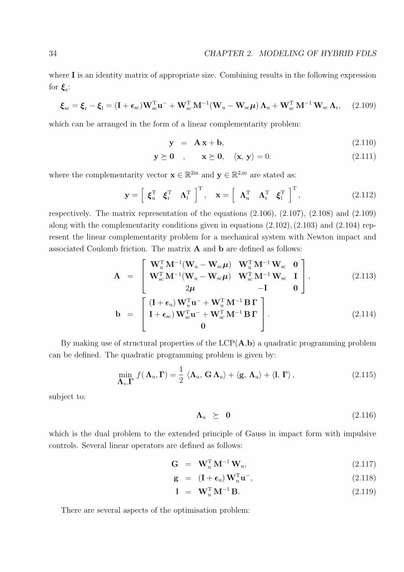
34 CHAPTER 2. MODELING OF HYBRID FDLS
where I is an identity matrix of appropriate size. Combining results in the following expression
for ξs:
ξsc = ξr − ξl = (I + εsc)WTscu
− + WTsc M
−1(Wu −Wscµ)Λu + WTsc M
−1 Wsc Λr, (2.109)
which can be arranged in the form of a linear complementarity problem:
y = Ax + b, (2.110)
y º 0 , x º 0, 〈x, y〉 = 0. (2.111)
where the complementarity vector x ∈ R2m and y ∈ R2,m are stated as:
y =[
ξTu ξT
r ΛTl
]T
, x =[
ΛTu ΛT
r ξTl
]T
, (2.112)
respectively. The matrix representation of the equations (2.106), (2.107), (2.108) and (2.109)
along with the complementarity conditions given in equations (2.102), (2.103) and (2.104) rep-
resent the linear complementarity problem for a mechanical system with Newton impact and
associated Coulomb friction. The matrix A and b are defined as follows:
A =
WTu M−1(Wu −Wscµ) WT
u M−1 Wsc 0
WTsc M
−1(Wu −Wscµ) WTsc M
−1 Wsc I
2µ −I 0
, (2.113)
b =
(I + εu)WTu u− + WT
u M−1 BΓ
I + εsc)WTscu
− + WTsc M
−1 BΓ
0
. (2.114)
By making use of structural properties of the LCP(A,b) a quadratic programming problem
can be defined. The quadratic programming problem is given by:
minΛu,Γ
f(Λu,Γ) =1
2〈Λu, GΛu〉+ 〈g, Λu〉+ 〈l, Γ〉 , (2.115)
subject to:
Λu º 0 (2.116)
which is the dual problem to the extended principle of Gauss in impact form with impulsive
controls. Several linear operators are defined as follows:
G = WTu M−1 Wu, (2.117)
g = (I + εu)WTu u−, (2.118)
l = WTu M−1 B. (2.119)
There are several aspects of the optimisation problem:

2.4. UNDERACTUATED MANIPULATORS WITH IMPACTIVE BLOCKING 35
• In stating the optimisation problem for extended principle of Gauss in impactive form
and impulsive control form, it is assumed that kinematic and geometric compatibility is
given.
• The solution to the problem in (2.80) is unique if and only if G is positive definite, which
is only the case if the matrix of generalised contact force directions Wu has full rank.
(Since M−1 is always PD).
• Except kinematic and geometric compatibility, the existence of QP is dependent on wether
the linear operator A is bisymmetrical or not. The bisymmetry of the linear operator is
maintained if all µi’s in (2.94) are zero. This means that all impactive interactions in the
tangential contact direction are decoupled form the normal contact interaction.
2.4 Modeling Underactuated Manipulators with
Impactively Blockable Degrees of Freedom
The physical realisation of impactive blocking is achieved in several ways, however its modeling
can be seen as a Coulomb like friction force characteristics with controlled/adjustable height
of the set-valued signum relation. In order for the blocking action to take place, the height
of the set-valued signum relation must rise high enough to reduce the relative velocity to zero
immediately and must be zero if unblocked. This relation between a bilateral perfect constraint
and free direction of motion is shown graphically in figures 2.5 and 2.7. In the sequel a class
of mechanical systems are modeled and investigated, in which the only impulsive action is
generated by the control action and it is assumed that there are no contact interactions with
the surroundings. This class of mechanical systems have blockable DOF, which is described
by an impulsive set-valued control law. Set-valued force elements are used in order to derive
the complementarity structure of the blocking control. The relevance of unilateral analysis
in mechanics is therefore closely related to the set-valued impulsive control of systems with
blockable DOF. Set-valued force laws in mechanics are treated systematically in [44] by Glocker.
In references [62] and [61] by Moller et al. the extension of the set-valued force law analysis to
basic elements in electrical circuits can be found. The result of this subsection as presented in
equations (2.166) to (2.172) is already stated in [115] and [116] by Yunt et al. as a result and
used in the NLP methods. A practical introduction to the concept of MDI in the framework
of impulsive control is provided in [110] by Yunt.
The dynamics of a mechanical system with n degrees of freedom, p blockable directions of
motion and s Lebesgue measurable controls is formulated as a measure-differential inclusion as

36 CHAPTER 2. MODELING OF HYBRID FDLS
follows:
M(q(t)) du − h(q(t),u(t+)) dt−B(q(t)) dΓ = 0, (2.120)
−dΓbi∈ dNi Sgn(γ+
bi), ∀ i ∈ IB, (2.121)
|γ+bi| ∈ Upr (dNi) , ∀ i ∈ IB, (2.122)
τ ∈ Cτ . (2.123)
Here q(t) and u(t+) denote the absolutely continuous (AC) generalised positions and right
continuous locally bounded variation (RCLBV) generalised velocities, respectively. The set of
all blockable DOF is denoted by IB. The linear operator M(q) ∈ Rn×n is the mass matrix,
h(q,u) ∈ Rn×1 denote the vector of gyroscopical, centripetal and coriolis, smooth potential
(gravity, spring etc.) forces and dΓ ∈ Rs×1 is the differential measure of controls which can
be unbounded, set-valued and impulsive. The set Cτ denotes the bounds on the Lebesgue-
measurable single-valued ordinary controls, and is assumed to be of box-constrained type. The
matrix B(q) ∈ Rn×s includes the generalised control directions. This representation is the
maximal representation, meaning that all joints are unblocked. The relative joint velocity at
any blockable direction is a linear combination of the generalised velocities for scleronomic
mechanical systems and is given by (2.124):
γbi= wbi
(q)u, ∀ i ∈ IB. (2.124)
For such a Lagrangian system a n-dimensional vector γ ∈ Rn is defined:
γ = WT(q)u, (2.125)
where γ ∈ Rp such that wbi(q) ∈ colW,∀i ∈ IB and W ∈ Rn×p. Here col· denotes
the set of column vectors of the relevant linear operator. Without loss of generality, one can
assume colW ⊆ colB if n ≥ p. By the inclusion colW ⊆ colB, the compactness of Cτ
and the unboundedness of dΓb the relation:
dΓ = dΓb + τ dt, (2.126)
is tractable.
2.5 Complementarity Description of the Set-valued Im-
pulsive Blocking Control Action
Blocking is investigated in two dimensions. The first dimension incorporates the action of
blocking itself where a relative velocity is reduced immediately to zero. The second dimension

2.5. COMPLEMENTARITY DESCRIPTION OF IMPULSIVE BLOCKING 37
is the action of keeping blocked. The first dimension involves impulsive control that acts on
the system at an instant and the second one a conventional control action on force level over an
interval such that a relative velocity i.e. relative acceleration is kept zero. The impulsive and
the conventional control action have set-valued character, in the sense that beyond a threshold
that is necessary to block impactively or to keep blocked, any arbitrary value of the impulsive
and conventional blocking control action is possible in the complementarity framework. The
impulsive set-valued blocking control law is described by the two set-valued relations in (2.121)
and (2.122) which are depicted in figures 2.6 and 2.9. The differential measure of the normal
control force can be seen as composed of a Lebesgue measurable and a Borel measurable part.
In this case, relation (2.122) is visualised as in the figures 2.8 and 2.9. The differential measures
of the normal control force dN, right normal control force dNr and left normal control force
dNl are decomposed into Lebesgue and Borel measurable parts as given in equations (2.127) to
(2.129):
dN = n dt + N′ dσ = n dt + (N+ − N−) dσ, (2.127)
dNr = nr dt + N′r dσ = nr dt + (N+
r − N−r ) dσ, (2.128)
dNl = nl dt + N′l dσ = nl dt + (N+
l − N−l ) dσ. (2.129)
Here N′, N′r and N′
l denote the Radon-Nykodym derivatives of dN, dNr and dNl, respectively.
The differential measures of the blocking control force dΓ, right normal control force dΓr and
left normal control force dΓl are decomposed into Lebesgue and Borel measurable parts as given
in equations (2.130) to (2.132):
dΓb = τb dt + Γ′b dσ = τb dt + (Γ+b − Γ−b ) dσ, (2.130)
dΓbr = τbr dt + Γ′br dσ = τb dt + (Γ+br − Γ−br) dσ, (2.131)
dΓbl = τbl dt + Γ′bl dσ = τb dt + (Γ+bl − Γ−bl) dσ. (2.132)
Here Γ′, Γ′br and Γ′bl denote the Radon-Nykodym derivatives of dΓ, dΓbr and dΓbl, respectively.
The evaluation of the Lebesgue-Stieltjes integral of dN and dΓ over an atomic instant of time
where an impulsive control action is applied on the system yields:
∫
tidN = N+ − N− = N, (2.133)
∫
tidΓb = Γ+
b − Γ−b = Γb, (2.134)
respectively. The entities N and Γb are denoted by impulsive normal blocking force and impul-
sive control force. The decomposition of the UPR (unilateral primitive)-type relation between
|γ+b | and N, into two UPR relations as depicted in figure 2.6 is expressed by set of relations

38 CHAPTER 2. MODELING OF HYBRID FDLS
tt t
n n n = 0> > 0
8
(a) (b) (c)
8
Figure 2.5: (a) A perfect bilateral constraint is equivalent to a normal control force that
takes infinite values, (b) For values of N less than infinity and greater zero, the blocking
action has friction characteristics, (c) if n = 0 there is no braking force.
(2.135) to (2.138):
N = Nr + Nl, (2.135)
γ+b = γ+
br − γ+bl, (2.136)
γ+br Nr = 0, Γ+
br ≥ 0, Nr ≥ 0, (2.137)
γ+bl Nl = 0, Γ+
bl ≥ 0, Nl ≥ 0. (2.138)
In a nonimpactive phase of motion, the action of keeping blocked or applying no blocking force
is formulated as an UPR between | γ+b | and N. The decomposition of the UPR-type relation
between | γ+b | and N, into two UPR relations as depicted in figure 2.11 is expressed by set of
relations (2.139) to (2.142):
n = nr + nl, (2.139)
γ+b = γ+
br − γ+bl, (2.140)
γ+br nr = 0, γ+
br ≥ 0, nr ≥ 0, (2.141)
γ+bl nl = 0, γ+
bl ≥ 0, nl ≥ 0. (2.142)
The relations given in (2.135) to (2.138) are equivalently expressed as:
γ+b = γ+
br − γ+bl, (2.143)
γ+bl N = 0, Γ+
bl ≥ 0, N ≥ 0, (2.144)
γ+br N = 0, Γ+
br ≥ 0, N ≥ 0. (2.145)

2.5. COMPLEMENTARITY DESCRIPTION OF IMPULSIVE BLOCKING 39
Figure 2.6: The set-valued signum relation and its decomposition into two unilateral
primitives that represents relation between the discretised differential measure of normal
blocking force to the discretised differential measure of the control force.
The relations given in (2.139) to (2.142) are equivalently expressed as:
γ+b = γ+
br − γ+bl, (2.146)
γ+bl n = 0, γ+
bl ≥ 0, n ≥ 0, (2.147)
γ+br n = 0, γ+
br ≥ 0, n ≥ 0. (2.148)
The figure 2.6 shows the relation between the differential measures of normal control force
and the blocking control force. It depicts the decomposition of the set-valued signum charac-
teristics into two unilateral primitives graphically, which are stated in the relations (2.149) to

40 CHAPTER 2. MODELING OF HYBRID FDLS
Figure 2.7: (a) If N rises to infinity, the relative velocity in the next moment drops to zero,
(b) For values of N less than infinity and greater zero, the blocking action has friction
characteristics with respect to the relative velocity, (c) if N = 0 there is no blocking in the
next moment.
Upr( )
n
gb+
gb+
Figure 2.8: The unilateral primitive
about the relation of the blocking
normal force to the relative acceleration
γ+b .
Upr( )
gb+
gb+
N N+
Figure 2.9: The UPR about the relation
of the differential measure of blocking
normal impulsive force to the relative
velocity γ+b ∈ RCLBV .

2.5. COMPLEMENTARITY DESCRIPTION OF IMPULSIVE BLOCKING 41
+
Upr( ) Upr( )
N
N Nl Nr
NrNl
Figure 2.10: The decomposition of the Upr relation in figure 2.9 into two unilateral
primitives.
n
n nl
n r+
Upr( ) Upr( )
n rn
l
Figure 2.11: The decomposition of the Upr relation in figure 2.8 into two unilateral
primitives.

42 CHAPTER 2. MODELING OF HYBRID FDLS
(2.153):
Γbri = Γbi+ Ni, ∀ i ∈ IB, (2.149)
Γbli = −Γbi+ Ni, ∀ i ∈ IB, (2.150)
γ+bi
= γ+bri− γ+
bli∀ i ∈ IB, (2.151)
γ+bri
Γbri = 0, Γbri ≥ 0, γ+bri≥ 0, ∀ i ∈ IB, (2.152)
γ+bli
Γbli = 0, Γbli ≥ 0, γ+bli≥ 0 ∀ i ∈ IB. (2.153)
In a nonimpactive phase of motion, the signum characteristics is expressed by the set of
relations (2.154) to (2.158):
τbr = τb + n, (2.154)
τbl = −τb + n, (2.155)
γ+b = γ+
br − γ+bl, (2.156)
γ+br τbr = 0, γ+
br ≥ 0, τbr ≥ 0, (2.157)
γ+bl τbl = 0, γ+
bl ≥ 0, τbl ≥ 0. (2.158)
The relations given from (2.143) to (2.145) and from (2.149) to (2.153) are combined in (2.159)
to (2.165) to reformulate the impulsive set-valued blocking control law given in equations (2.121)
and (2.122) in the complementarity framework:
Γbri = Γbi+ Ni, ∀ i ∈ IB, (2.159)
Γbli = −Γbi+ Ni, ∀ i ∈ IB, (2.160)
γ+bi
= γ+bri− γ+
bli∀ i ∈ IB, (2.161)
γ+bri
Γbri = 0, Γ+bri≥ 0, Γbri ≥ 0, ∀ i ∈ IB, (2.162)
γ+bli
Γbli = 0, Γ+bli≥ 0, Γbli ≥ 0, ∀ i ∈ IB, (2.163)
γ+bri
Ni = 0, Γ+bri≥ 0, Ni ≥ 0, ∀ i ∈ IB, (2.164)
γ+bli
Ni = 0, Γ+bli≥ 0, Ni ≥ 0, ∀ i ∈ IB. (2.165)
In a similar way, the behaviour of the set-valued controls in the absence of impulsive action
is captured by the combination of the relations given from (2.146) to (2.148) and from (2.154)
to (2.158) are combined in (2.166) to (2.172) in order to reformulate the set-valued blocking

2.5. COMPLEMENTARITY DESCRIPTION OF IMPULSIVE BLOCKING 43
q1
q2
MS
1
P2
Figure 2.12: The 2-DOF linear mechanism
control in the complementarity framework on acceleration level:
τbri = τbi+ ni, ∀ i ∈ IB, (2.166)
τbli = −τbi+ ni, ∀ i ∈ IB, (2.167)
γ+bi
= γ+bri− γ+
bli, ∀ i ∈ IB, (2.168)
γ+bri
τbri = 0, γ+bri≥ 0, τbri ≥ 0, ∀ i ∈ IB, (2.169)
γ+bli
τbli = 0, γ+bli≥ 0, τbli ≥ 0, ∀ i ∈ IB, (2.170)
γ+bri
ni = 0, γ+bri≥ 0, ni ≥ 0, ∀ i ∈ IB, (2.171)
γ+bli
ni = 0, γ+bli≥ 0, ni ≥ 0, ∀ i ∈ IB. (2.172)
This modeling approach of set-valued impulsive blocking control is published in [115] by Yunt
et al..
2.5.1 A Case Study
At this point it is appropriate to illustrate this characteristic by making use of an example
mechanical system. The example mechanical system is a linear planar mechanical system with
two-degrees of freedom (DOF) as depicted in figure 2.12. One DOF of the system is fully
actuated and the inclined link can only be commanded by frictional braking. This example is
considered as the most simple nonsmooth underactuated mechanical system with explicit phase
transitions. The time-optimal control problem of this measure-differential inclusion is stated

44 CHAPTER 2. MODELING OF HYBRID FDLS
as follows:
min tf (2.173)
subject to boundary constraints
q1(tf) = q1f , q2(tf) = q2f , u1(tf) = u1f , u2(tf) = u2f ,
Set-Valued Mixed Lebesgue-Borel type Control Constraints
dΛs ∈ −dΓ Sgn(ξs),
Constraints on the ordinary control
τmin ≤ τ ≤ τmax ∀ t,
(2.174)
and to the dynamics in measure-differential equation form:
[m1 + m2 m2 cos(α)
m2 cos(α) m2
] [du1
du2
]=
[τ dt
dΛs
]. (2.175)
where ξs is given by ξs = u+2 + εs u−2 . Without loss of generality the tangential restitution
coefficient is taken zero. The friction law is decomposed into two upper primitives resulting in
two sets of complementary relations. These relations are given by:
u+2 = ξr − ξl, (2.176)
dΛs = dΛr − dΛl, (2.177)
dΓ = dΛr + dΛl, (2.178)
dΛr ≥ 0, dΛl ≥ 0, (2.179)
ξr ≥ 0, ξl ≥ 0, (2.180)
ξr dΛr = 0, ξl dΛl = 0, (2.181)
ξr dΓ = 0, ξl dΓ = 0. (2.182)
By making use equations (2.176), (2.177), (2.178) several variables in the complementarities in
(2.181) and (2.182) are eliminated.

2.6. IMPACTIVE UNDERACTUATED MANIPULATORS 45
2.6 Passively Actuated Robotic Manipulators with block-
able DOF
The difference in the structure of the equations of motion in different phases of motion arises
from dimension of admissible variations. The representation of rigid-body mechanical dynami-
cal systems can be adjusted in three ways to a change in the dimension of admissible variations
as summarised below:
• The number of algebraical equations in the differential-algebraical representation can be
changed. In this case there exists a set of algebraic equations that have to be fulfilled
during the integration of the differential equations.
• A new set of generalised coordinates can be selected, to eliminate the necessity of taking
care of the algebraical constraints.
• The equations of motion can be projected to a subspace such that the dynamics do not
evolve in the restrained directions of motion, without changing the number of generalised
coordinates or generating additional algebraical constraints.
The modeling approach presented in this section is published in short form in [111] by Yunt.
2.6.1 Post-transition Equations of Motion and Discontinuity Con-
ditions
The assumptions during a possibly impactive transition are given as follows:
• The transitions which involve blocking a relative joint DOF may be impactively, which
arises from fully inelastic impacts.
• The generalised position remains unchanged during transition.
• The impulsive control action, when triggered reduces the post-impact relative joint ve-
locity to zero.
Further, the height of the set-valued signum relation must be high enough to reduce the relative
velocity to zero immediately and must be zero if unblocked. Let n is the total number of degrees
of freedom of the robotic manipulator. The equations of motion are given by:
M(q) u− h(q,u)−B(q) τ = 0, (2.183)
where q and u denote the absolutely continuous generalised positions and bounded variation
generalised velocities, respectively. Here M(q) ∈ Rn×n is the mass matrix, h(q,u) ∈ Rn×1

46 CHAPTER 2. MODELING OF HYBRID FDLS
denote the vector of gyroscopical and coriolis, smooth potential (gravity, spring etc.) forces
and τ ∈ Rs×1 are the controls which can be set-valued. The linear operator B(q) ∈ Rn×s
includes the generalised control directions. This representation is the maximal representation,
meaning that all joints are unblocked. The relative joint velocity at any joint is given by (2.184):
γi = wTi (q)u. (2.184)
For such a Lagrangian system a n dimensional vector γ ∈ Rn is defined:
γ = WT(q)u, (2.185)
such that wi(q) ∈ colW and W ∈ Rn×n. Here col· denotes the set of column vectors of the
relevant linear operator. In order to describe the transition condition at any ti ∈ IT properly
following index sets are defined:
CBi= i |γ+
i = 0, γ+i = 0,∀t ∈ (
t+i , t−i+1
),CPi
= i |γ+i = 0, γ+
i ∈ R.Here CBi
denotes the index set of joints that remain blocked after a transition time until another
possible transition time. The set CPiis the index set of joints at which a blocking action takes
place at a transition time, such that the relative post-transition joint velocity is nullified. Let
CPi\Bibe defined as:
CPi\Bi= i | i ∈ CPi
, i /∈ CBi. (2.186)
For convenience it is assumed that CPi\Bi= ∅ without loss of generality. Let p < s the number
DOF which are being blocked impactively. The impact equation is given by the following
expression:
M(q) (u+ − u−)−Wb(q)Γ = 0, (2.187)
where Γ ∈ Rp are blocking impulses that can be generated at the joints, which participate in
blocking and the matrix Wb ∈ Rn×p denotes the generalised force direction of the blocking
forces, such that colWb ⊂ colB. Further, it is assumed that colB ⊂ colW for conve-
nience and without loss of generality. The difference between the pre-impact and post-impact
relative joint contact velocities is related to the post-, and pre-impact generalised velocities of
the mechanical system by expression (2.188):
γ+ − γ− = WT(q) (u+ − u−). (2.188)
Let at a transition, which is accompanied by an impact, which is induced by the sudden blocking
of directions of motion, p of the joints, characterised by their force directions, be active. Then,
the vector γ can be decomposed in the following manner:
γ+b
· · ·γ+
f
−
γ−b· · ·γ−f
=
[Wb
... Wf
]T
(u+ − u−), (2.189)

2.6. IMPACTIVE UNDERACTUATED MANIPULATORS 47
where γ+b and γ−b denote the relative joint post-, and pretransition velocities at the blocked/active
joints, and γ+f and γ−f denote the relative joint post-, and pretransition velocities at the
free/passive joints. Here Wb ∈ Rn×p, Wf ∈ Rn×(n−p) denote the matrices, consisting column-
wise of blocked and unblocked generalised directions such that colWf⋃
colWb = colWand colWf
⋂colWb = ∅. The equation (2.187) can be solved for the jump in the gener-
alised velocities of the system:
u+ − u− = M−1(q)Wb(q)Γ. (2.190)
Inserting this expression in (2.188) reveals the jump in the vector of relative joint velocity
vector:
γ+ − γ− = WT(q) (u+ − u−) = WT M−1 W
Γ
· · ·∆
. (2.191)
By making use of the decomposition of the relative joint velocities into blocked and free direc-
tions as introduced in equation (2.189) following is obtained:
γ+b − γ−b· · · · · ·
γ+f − γ−f
=
WTb M−1 Wb
... WTb M−1 Wf
· · · · · · · · · · · · · · · · · · · · · · · · · · · · · · · · · · · ·WT
f M−1 Wb... WT
f M−1 Wf
Γ
· · ·∆
. (2.192)
In order to simplify the notation matrices Gbb, Gb f , Gfb and Gf f are introduced as follows:
γ+b − γ−b· · · · · ·
γ+f − γ−f
=
Gbb... Gb f
· · · · · · · · · · · · · · · · · ·Gfb
... Gf f
Γ
· · ·∆
. (2.193)
The blocking at every direction is induced by a single control direction. Further, immediately
after blocking action the post-impact relative velocity γ+ immediately reduces to zero. Given
these two assumptions the impulse at contacts which do not participate at the blocking and
post-transition velocity at the blocked joints are zero, as stated below:
∆ = 0, (2.194)
γ+b = 0. (2.195)
The impulse vector Γ can be eliminated after insertion of (2.194) and (2.195) into (2.193),
which boils down to:
−γ−b = GbbΓ, (2.196)
γ+f − γ−f = GfbΓ. (2.197)

48 CHAPTER 2. MODELING OF HYBRID FDLS
Equation (2.196) when solved for Γ reveals:
Γ = −G−1bb γ−b , (2.198)
and insertion into equation (2.197) eliminates the impulse and establishes the relation between
post-, and pre-impact relative joint velocities:
γ+f = γ−f −Gfb G−1
bb γ−b . (2.199)
This equation can be rewritten in terms of the post-, and pre-impact generalised velocities by
making use of equation (2.189) as given in (2.200):
WTf u+ = WT
f u− −Gfb G−1bb WT
b u−, (2.200)
and by defining K(q) = WTf −Gfb G−1
bb WTb reveals following expression:
WTf (q)u+ −K(q)u− = 0. (2.201)
On the other hand by insertion of the impulse obtained in (2.198) into (2.190) reveals the
relation between post- and pretransition generalised velocities:
u+ − u− = −M−1 WbG−1bb WT
b u−. (2.202)
This equation can be rewritten in the following form:
u+ = (I −M−1 WbG−1bb WT
b )u− = PT⊥(q)u−. (2.203)
The value of impulse established in (2.198) represents the minimal value to induce full blocking
at joint i ∈ CBi.
2.6.2 Lagrangian Dynamics in Different Phases of Motion
After the possibly impactive transition the equations of motion on acceleration level may differ
from the pre-transition equations of motion based on the closed directions of motion. It is
assumed that the interaction of the Lagrangian system with the surroundings (unilateral con-
tacts, etc. ) do not interfere during the course of control action. The generalised acceleration of
the finite-dimensional Lagrangian system when some DOF are closed by τ b, is given by (2.204)
on acceleration level:
u = M−1(q)h(q,u) + M−1(q)Wb(q) τ b + M−1(q)B(q) τ . (2.204)
The controls τ b represent the forces which are required to constrain the vector field from
evolving in the direction γb. The linear operator Wb denotes the generalised force direction

2.6. IMPACTIVE UNDERACTUATED MANIPULATORS 49
of the constraining forces, such that colWb ⊂ colB. The acceleration γb in the blocked
directions must vanish, which means that:
γb = WTb u + WT
b u = 0 . (2.205)
The insertion of equation (2.204) in equation (2.205) reveals:
WTb u + WT
b u = WTb M−1h + WT
b M−1Wb τ b + WTb M−1B τ + WT
b u = 0 . (2.206)
The equation (2.206) can be solved for the blocking forces/moments as below:
τ b = −(WTb M−1Wb)
−1(WT
b M−1h + WTb M−1B τ + WT
b u)
. (2.207)
Defining the projector P‖ as
P‖ = Wb(WTb M−1Wb)
−1WTb M−1 (2.208)
and inserting into equation (2.204) reveals the projected dynamics:
Mu− h−P‖ (h + B τ ) + Wb(WTb M−1Wb)
−1WTb u−B τ = 0 . (2.209)
The equations of motion after the directions Wb are closed in the generalised coordinates can
be rearranged as below:
Mu−P⊥ h−P⊥B τ + Wb(WTb M−1Wb)
−1WTb u = 0 . (2.210)
The new vector of coriolis and gyroscopical forces as well as the linear operator of generalised
control directions can be redefined as:
hb = P⊥ h−Wb(WTb M−1Wb)
−1WTb u , (2.211)
Bb = P⊥B, (2.212)
where the orthogonal projector P⊥ to P‖ is defined as
P⊥ = I−P‖, (2.213)
with I being an identity matrix of appropriate size. So the Lebesgue measurable projected
dynamics in n degrees of freedom can be stated as:
M(q) u− hb(q,u)−Bb(q) τ = 0 . (2.214)

50 CHAPTER 2. MODELING OF HYBRID FDLS
2.6.3 Change in Mechanical Energy and Impuls and Dissipation
The Lagrangian of FDLS is defined as:
L(q,u) = T (q,u)− V (q) (2.215)
Here T (q,u) denotes the total kinetic, and V (q) the total smooth potential energy of the
system. The total energy of the system is:
H(q,u) = T (q,u) + V (q). (2.216)
The differential measure of the energy H is given by:
dH(q,u) =dH
dtdt +
(T+ − T−)
dσ (2.217)
If the Lebesgue-Stieltjes Integral of the differential measure of the total energy H over an atomic
time instant is evaluated then one obtains:
∫
tidH = T+ − T−. (2.218)
The Borel measurable part of H is related to the jump in kinetic energy:
T+ − T− =1
2
⟨u+, M(q)u+
⟩− 1
2
⟨u−, M(q)u−
⟩, (2.219)
and is nonzero if and only if there is an impulsive action that induces a jump in the generalized
velocities. The energy dissipation during an impactive transition is given by:
1
2
(⟨u+,M(q)u+
⟩− ⟨u−,M(q)u−
⟩)= (2.220)
1
2
⟨PT⊥u
−, M(q)PT⊥u
−⟩− 1
2
⟨u−,M(q)u−
⟩=
1
2
⟨(P⊥ − I)T u−,M(q)
(PT⊥ + I
)u−
⟩
= −1
2
⟨WT
b u−,G−1bb WT
b u−⟩
(2.221)
= −1
2
⟨γ−b ,G−1
bb γ−b⟩. (2.222)
Given this setting a straight-forward calculation shows that the change in total momentum L
is given by:
L+ − L− = M(q)(u+ − u−) = M(q)(PT⊥ − I
)u− = −M(q)PT
‖ u− = −WbG
−1bb WT
b u−.
(2.223)

2.6. IMPACTIVE UNDERACTUATED MANIPULATORS 51
ex
ey
a m l1
Q11
m l2
Q2 2
O
S1
bI
I
d1
d2
S2
m4
Q4
m3
Q3
A
Figure 2.13: Planar double pendulum with one impactively blockable degrees of freedom.
2.6.4 Example: Planar Double Pendulum with One Blockable DOF
The example mechanical system can be seen in fig. 2.13. The system has two degrees of
freedom, namely, α and β. The DOF α is measured with respect to the coordinate frame I.
The DOF β denotes the relative angular position of the second link with respect to the first link.
The first link is actuated by a motor at point O, is controlled continuously by single-valued,
ordinary controller. The second link can be blocked by a brake at the axis, where both links
join each other. This control action is set-valued, impulsive and discontinuous. The center of
mass of each link is located at positions S1 and S2. The symbols m, l and Θ denote the mass,
length and inertia moments of the respective link, where following parameters are defined:
p1 = m1 d21 + m2 l21 + m2 d2
2 + Θ1 + Θ2,
p2 = 2 m2 l1 d2, p3 = m2 d22 + Θ2,
p4 = m2 l1 d2, p5 = m2 d22 + Θ2,
p6 = (p3 p2 − p24), p7 = −2 p4 p5,
p8 = p3 p1 − p25.
where the positions of the center of masses of the links are given by:
IrS1 =
d1 sin(α)
d1 cos(α)
0
, IrS2 =
l1 sin(α) + d2 sin(α + β)
l1 cos(α) + d2 cos(α + β)
0
, (2.224)

52 CHAPTER 2. MODELING OF HYBRID FDLS
and the velocities of the center of masses are obtained by direct time differentiation:
IvS1 =
d1 cos(α)α
−d1 sin(α)α
0
(2.225)
IvS2 =
(l1 cos(α) + d2 cos(α + β)) α + d2 cos(α + β)β
(−l1 sin(α)− d2 sin(α + β)) α− d2 sin(α + β)β
0
. (2.226)
The angular velocities of the links are given by:
IωS1 =
0
0
α
, IωS2 =
0
0
β + α
. (2.227)
The total kinetic energy of the manipulator is:
T =1
2(p1 + p2 cos(β)) α2 +
1
2p3 β2 + α β (cos(β)p4 + p5) . (2.228)
The equations of motion are given by:
[p1 + p2 cos(β) cos(β)p4 + p5
cos(β)p4 + p5 p3
][α
β
]−
[sin(β)
(p2 α + β p4
)β
−12p2 sin(β)α2
]−
[τ
λs
]= 0.
(2.229)
The generalised force directions are given by:
Wb =[
0 1]T
, Wf =[
1 0]T
. (2.230)
The terms for Gbb, Gbf , Gfb, Gff are given by:
Gbb =p1 + p2 cos(β)
p6 (cos(β))2 + p7 cos(β) + p8
, (2.231)
Gbf =− cos(β)p4 − p5
p6 (cos(β))2 + p7 cos(β) + p8
= Gfb, (2.232)
Gff =p3
p6 (cos(β))2 + p7 cos(β) + p8
. (2.233)
The linear operator K is as follows:
K =[
1 cos(β)p4+p5
p1+p2 cos(β)
], (2.234)

2.6. IMPACTIVE UNDERACTUATED MANIPULATORS 53
Given this setting, the dissipated energy in the system in case of blocking the underactuated
second link and the change in the total momentum amounts to:
∆T = −p6 (cos(β))2 + p7 cos(β) + p8
2(p1 + p2 cos(β))β(t−i )2, (2.235)
and
∆L = −[
0
1
]Gbb
[0 1
] [α(t−i )
β(t−i )
]= −
[0
p1+p2 cos(β)
p6 (cos(β))2+p7 cos(β)+p8
]β(t−i ) (2.236)
respectively. The projector in (2.203) becomes in this case:
PT⊥ =
[1 (cos(β) p4 + p5)/(p1 + p2 cos(β))
0 0
]. (2.237)

54 CHAPTER 2. MODELING OF HYBRID FDLS
.

Chapter 3
Numerical Methods for the Trajectory
Optimisation of Hybrid
Finite-Dimensional Lagrangian
Systems
The numerical treatment of optimal control of hybrid finite-dimensional Lagrangian systems
(HFDLS) belongs to the applied mathematics branch of Mathematical Programs with
Equilibrium Constraints (MPEC). This chapter commences with the definitions and classes
of MPECs and the discussion of the features of the TOHLS from the perspective of MPEC.
Both methods are based on augmented Lagrangian methods and therefore a section is devoted
to different numerical methods in solving MPECs with emphasis placed on the augmented La-
grangian approach. Given the importance of complementarity problems in section 3.1 a general
overview is provided. There is already a vast literature for dealing with the solution of NLP’s
that have variational inequality type constraints. The key to the solution of such problems
are reformulations, which rely on proposing suitable classes of functions with the aid of which
one can reformulate NCP’s or LCP’s as equality constraints. Because of the importance of
reformulation functions in section 3.1 several such functions are discussed. The existence and
uniqueness of the dual multipliers and the normality of the nonlinear programming problem
is discussed in the sequel for the type of MPEC that arise from the trajectory optimisation
of hybrid finite-dimensional structure-variant Lagrangian systems. Based on this analysis two
numerical methods are introduced. To the best knowledge of the author the augmented La-
grangian method is first used in the framework of this thesis in the nonsmooth approach to
MPEC.
In [73] a MPEC is defined as an optimisation problem in which the essential constraints
are defined by parametric variational inequality or complementarity systems. One of the many
55

56 CHAPTER 3. NUMERICAL METHODS FOR FDLS
representations of a MPEC is stated in abstract form as follows:
minx,z
f(x, z), (3.1)
z ∈ S(x), (3.2)
x ∈ Uad, z ∈ Z. (3.3)
The problem stated in (3.1) to (3.3) includes a subclass of so-called bilevel programs, where
S assigns each x ∈ Uad the solution of a ”lower-level” optimisation problem. In the case where
the complementarity system arises from FDLS without Coulomb-type friction force interaction,
a so-called subclass of MPEC, namely, bilevel programs apply. In [63] by Moreau it has been
shown that the determination of the accelerations of a mechanical system subject to unilateral
constraints without friction can be represented as a dual quadratic programming problem. Fur-
ther, it is shown that the generalisation of the Gauss’ variational principle is valid in the case of
unilateral constraints without friction. Glocker showed that a quadratic programming problem
is obtained if Tresca type friction, where the normal force is decoupled from the tangential
force, exists. For the case of controlled nonsmooth Lagrangian systems the optimisation prob-
lem takes the form as described by relations (2.78) to (2.81), which is the dual of the extended
principle of Gauss in control form. Here the bilevel programming structure requires to find
the active contact forces for given control forces τ . The control forces at every instant repre-
sent the variables of the higher level optimisation problem and the contact forces represent the
lower level optimisation variables. To find an optimal trajectory for such a mechanical problem
means embedding a quadratic programming problem in every instant of time. The equations of
motion along with the linear-complementarity conditions constitute necessary Karush-Kuhn-
Tucker conditions of optimality for the quadratic programming problem that derives from the
extended principle of Gauss in the absence of Coulomb-type of friction. If Coulomb-type of
friction exists, then a QP can not be formulated any more because of the lack of the bisym-
metrical structure of the LCP (A,b). So if Coulomb type friction exists at the contacts, then
the optimal control problem is subject to variational inequalities and the mechanical quadratic
programming problem does not exist any more, which is a problem to be treated in a broader
class of problems, which require that at every instant of time the linear complementarity prob-
lem described by the relations (2.74) to (2.77) is solved. In the case of occurrence of impulsive
control and impulsive active contact forces, one can classify the impulsive control forces as
the primal variables of the MPEC, and the impulsive active contact forces as the secondary
variables of the mathematical program. If impulsive control forces and impulsive contact forces
are applied on the finite-dimensional Lagrangian system a dual problem in the impulsive forces
and controls is formulated if some requirements are fulfilled. These are:
• The choice of an impact law, that has the character of a constitutive law must be made,

57
in order to relate pre-impact velocities to post-impact velocities.
• The collision and impact configurations have to be geometrically, kinematically and ki-
netically consistent.
This optimisation problem which can be seen as the impulsive dual of the extended Gauss
Principle in control form has the same bilevel structure as the optimisation problem described
above on acceleration level, namely, the ”secondary variables” contact impulses are supposed to
be determined in dependence of the impulsive control action. The unification of both problems
is achieved by formulating the evolution of the mechanical dynamics subject to set-valued force
interactions with the surroundings and the impulsive set-valued actions of the control strat-
egy as a measure-differential inclusion. By analogy, the measure-differential inclusion, that
describes the dynamics as a balance of measures, can be considered as the necessary conditions
of a ”lower-level” optimisation problem represented by the saddle-region restraining set S. In
this setting, the differential measures of generalised velocities and the generalised positions, the
differential measures of the active contact forces are the secondary variables, whereas the dif-
ferential measure of controls constitute the higher level variables, which affect the solutions of
the subordinated optimisation problem. In all cases as mentioned above, the controls are con-
sidered as the variables of the ”higher-level” optimisation problem whereas the contact forces
and states are variables of the ”lower-level” (quasi-) optimisation problem. If, however, in any
of the mentioned forces entail Coulomb type forces then the determination of the differential
measures of the contact forces as well as the differential measures of velocities can not be for-
mulated as a QP problem with inequality constraints at every instant of time. By the presence
of Coulomb type friction and tangential-impact laws the variational inequalities that describe
the contact conditions do not resemble the Karush-Kuhn-Tucker conditions of a QP like prob-
lem any more. In this case, one is left with solving these variational inequalities which are
mostly represented as nonlinear complementarity problems (NCP) or linear complementarity
problems (LCP). Armed with the knowledge of the numerical techniques and the complemen-
tarity modeling to solve systems of equalities and inequalities involving variational inequalities,
mathematical programs with equilibrium constraints (MPECs) that arise from TOHLS and
given in the abstract setting in (3.1) to ( 3.3) is cast in the form below:
min f(x,y) (3.4)
subject to (x,y) ∈ Z ⊂ Rm+n, (3.5)
such that y solves VI(C(x),F(x, ·)), (3.6)
where x ∈ Rn, y ∈ Rm are decision variables, Z is a closed set, C is a set-valued mapping, and
f : Rm+n → R and F : Rm+n → Rm+n are given functions. Here the constraints state that the
variable y must be a solution to a variational inequality that is parameterised by x.
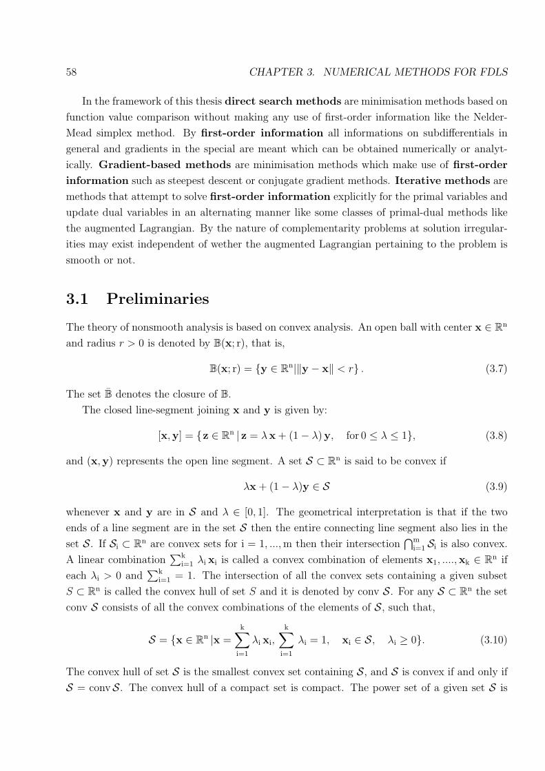
58 CHAPTER 3. NUMERICAL METHODS FOR FDLS
In the framework of this thesis direct search methods are minimisation methods based on
function value comparison without making any use of first-order information like the Nelder-
Mead simplex method. By first-order information all informations on subdifferentials in
general and gradients in the special are meant which can be obtained numerically or analyt-
ically. Gradient-based methods are minimisation methods which make use of first-order
information such as steepest descent or conjugate gradient methods. Iterative methods are
methods that attempt to solve first-order information explicitly for the primal variables and
update dual variables in an alternating manner like some classes of primal-dual methods like
the augmented Lagrangian. By the nature of complementarity problems at solution irregular-
ities may exist independent of wether the augmented Lagrangian pertaining to the problem is
smooth or not.
3.1 Preliminaries
The theory of nonsmooth analysis is based on convex analysis. An open ball with center x ∈ Rn
and radius r > 0 is denoted by B(x; r), that is,
B(x; r) = y ∈ Rn|‖y − x‖ < r . (3.7)
The set B denotes the closure of B.
The closed line-segment joining x and y is given by:
[x,y] = z ∈ Rn | z = λx + (1− λ)y, for 0 ≤ λ ≤ 1, (3.8)
and (x,y) represents the open line segment. A set S ⊂ Rn is said to be convex if
λx + (1− λ)y ∈ S (3.9)
whenever x and y are in S and λ ∈ [0, 1]. The geometrical interpretation is that if the two
ends of a line segment are in the set S then the entire connecting line segment also lies in the
set S. If Si ⊂ Rn are convex sets for i = 1, ..., m then their intersection⋂m
i=1 Si is also convex.
A linear combination∑k
i=1 λi xi is called a convex combination of elements x1, ....,xk ∈ Rn if
each λi > 0 and∑k
i=1 = 1. The intersection of all the convex sets containing a given subset
S ⊂ Rn is called the convex hull of set S and it is denoted by conv S. For any S ⊂ Rn the set
conv S consists of all the convex combinations of the elements of S, such that,
S = x ∈ Rn |x =k∑
i=1
λi xi,
k∑i=1
λi = 1, xi ∈ S, λi ≥ 0. (3.10)
The convex hull of set S is the smallest convex set containing S, and S is convex if and only if
S = convS. The convex hull of a compact set is compact. The power set of a given set S is

3.1. PRELIMINARIES 59
the set of all subsets of S and is denoted by P(S). A function f : Rn → R is said to be convex
if
f(λx + (1− λ)y) ≤ λ f(x) + (1− λ) f(y) (3.11)
whenever x and y are in Rn and λ ∈ [0, 1]. The f is said to be strictly convex if in equation
(3.11) strict inequality is valid on the open line-segment λ ∈ (0, 1).
Definition 3.1.1 A function f : Rn → R is locally Lipschitz continuous at x for any x ∈ Rn
with a positive constant L if there exists a positive number ε such that
|f(y)− f(z)| ≤ L‖y − z‖, ∀y, z ∈ B(x; ε). (3.12)
Lemma 3.1.1 A convex function is locally Lipschitz continuous at ∀x ∈ Rn.
Definition 3.1.2 A function f : Rn → R is positively homogeneous if
f(λx) = λ f(x) (3.13)
for all λ ≥ 0 and subadditive if
f(x + y) ≤ f(x) + f(y) (3.14)
for all x and y in Rn. A function is said to be sublinear if it is both positively homogeneous
and subadditive. A sublinear function is always convex.
Definition 3.1.3: Upper Semicontinuity A function f : Rn → R is said to be upper
semicontinuous at x ∈ Rn if for every sequence xk converging to x the following holds
lim supk→∞
f(xk) ≤ f(x). (3.15)
Definition 3.1.4: Lower Semicontinuity A function f : Rn → R is said to be lower
semicontinuous if
f(x) ≤ lim infk→∞
f(xk). (3.16)
Definition 3.1.5: Differentiability A function f : Rn → R is said to be differentiable at
x ∈ Rn if there exists a vector ∇f(x) ∈ Rn and a function ε : Rn → R such that for all d ∈ Rn
f(x + d) = f(x) +∇f(x)Td + ‖d‖ε(d). (3.17)
and ε(d) → 0 whenever ‖d‖ → 0.
Definition 3.1.6: Gradient The vector is called the gradient vector of the function f at
x and has the following formula
∇f(x) = (∂x
∂x1
, . . . ,∂x
∂xn
)T, (3.18)
where the components ∂x∂xi
, i = 1, . . . , n are called the partial derivatives of f .

60 CHAPTER 3. NUMERICAL METHODS FOR FDLS
Definition 3.1.7: Continuous Differentiability If the function is differentiable and all
the partial derivatives are continuous, then the function is said to be continuously differentiable
or smooth or equivalently,
f ∈ C1(Rn). (3.19)
Definition 3.1.8: Directional Derivative (Gateaux Derivative) The directional deriva-
tive of f at x ∈ Rn in the direction d ∈ Rn is defined as the following limit:
f ′(x;d) = limt↓0
f(x + td)− f(x)
t. (3.20)
The directional derivative is positively homogeneous and subadditive and hence sublinear as
a function of d. If a function f is differentiable at x, then the directional derivative exists in
every direction d ∈ Rn and
f ′(x;d) = 〈∇f(x), d〉 . (3.21)
If, in addition, f is convex, then for all y ∈ Rn
f(y) ≥ f(x) + 〈∇f(x), (y − x)〉 . (3.22)
Definition 3.1.9: Twice Differentiability A function f : Rn → R is twice differentiable
at x ∈ Rn if there exists a vector ∇f(x) ∈ Rn, a symmetric matrix ∇2f(x) ∈ Rn×n, and a
function ε : Rn → R such that for all d ∈ Rn
f(x + d) = f(x) + 〈∇f(x), d〉+1
2
⟨d, ∇2f(x)d
⟩+ ‖d‖2ε(d), (3.23)
where ε(d) → 0. The linear operator is called the Hessian matrix of the function f at x and is
defined to consist of second partial derivatives of f . If the function is twice differentiable and all
the second partial derivatives are continuous, then the function is said to be twice continuously
differentiable (f ∈ C2(Rn)).
Definition 3.1.10: Subdifferential the convex case The subdifferential of a convex
function f : Rn → R at x ∈ Rn is the set ∂ f(x) of vectors ξ ∈ Rn such that
∂ f(x) = ξ ∈ Rn | f(y) ≥ f(x) + 〈ξ, y − x〉 , ∀y ∈ Rn. (3.24)
Definition 3.1.11: Directional Derivative of a convex function Let f : Rn → R be a
convex function. Then the directional derivative f ′(x;d) exists in every direction d ∈ Rn and
it satisfies
f ′(x;d) = lim inft>0
f(x + td)− f(x)
t. (3.25)
Lemma 3.1.2 Let f : Rn → R be a convex function. Then for all x ∈ Rn
1. f ′(x;d) = max 〈ξ, d 〉 | ξ ∈ ∂ f(x), ∀d ∈ Rn,

3.1. PRELIMINARIES 61
2. ∂ f(x) = ξ ∈ Rn | f ′(x;d) ≥ 〈ξ, d 〉 ∀, d ∈ Rn.
Since for locally Lipschitz continuous functions there does not necessarily exist any classical
directional derivative, we first define a generalised directional derivative. Using this generalised
directional derivative the generalisation of the subdifferential to nonconvex locally Lipschitz
continuous functions can be formulated.
Definition 3.1.12: The Generalised Directional Derivative Let f : Rn → R be a
locally Lipschitz continuous function at x ∈ Rn. The generalised directional derivative of f at
x in the direction d ∈ Rn is defined by:
f o(x;d) = lim sup
y → x
t ↓ 0
f(y + td)− f(y)
t(3.26)
The generalised directional derivative always exists for locally Lipschitz continuous functions
and, as a function of d, it is sublinear.
Definition 3.1.13: The Generalised Subdifferential Let f : Rn → R be a locally
Lipschitz continuous function at x ∈ Rn. Then the subdifferential of f at x is the set ∂f(x) of
vectors ξ ∈ Rn such that
∂f(x) = ξ ∈ Rn | f o(x;d) ≥ 〈ξ, d 〉 ∀d ∈ Rn. (3.27)
Each vector ξ is called a subgradient of f at x.
The properties of the subdifferential are given as follows:
Lemma 3.1.3 Let f : Rn → R be a locally Lipschitz continuous function at x ∈ Rn with a
Lipschitz constant L. Then
1. f o(x;d) = max 〈ξ, d 〉 | ξ ∈ ∂f(x), ∀d ∈ Rn,
2. ∂f(x) is a nonempty, convex, and compact set such that ∂f(x) ⊂ B(0; L),
3. The mapping ∂f(x) : Rn → P(Rn) is upper semicontinuous.
The subdifferential for locally Lipschitz continuous functions is a generalisation of the subdif-
ferential for convex functions.
Theorem 3.1.1 (Rademacher) Let S ⊂ Rn be an open set. A function f : S → R that is
locally Lipschitz continuous on S is differentiable almost everywhere on S.
Proposition 3.1.1 Let f : Rn → R be locally Lipschitz continuous at x ∈ Rn. Then
∂f(x) = convξ ∈ Rn | there exists xi ⊂ Rn \Ωf such thatxi → x ∧ ∇ f(xi) → ξ . (3.28)
The set of points at which a given function f fails to be differentiable is denoted by Ωf .

62 CHAPTER 3. NUMERICAL METHODS FOR FDLS
x
Nepi f
x0+
epi f
f( )x
x0
f( )x0
x
n
epi fT+x0
n= -1
f( )x0
Figure 3.1: A nonconvex function f , its epigraph, and the Generalised Subdifferential at x0.
Definition 3.1.14: Generalised Jacobian Let a vector-valued function F : Rn → Rm be
given in component functions F(y) = [f1(y), . . . , fm(y)]. Let x be a point around which each
fi(y) is Lipschitz. Let JF(y) denote the usual m × n Jacobian matrix of partial derivatives
whenever y is a point at which the necessary partial derivatives exist. The generalised Jacobian
of F at y, denoted ∂F(y) is the convex hull of all m× n matrices Z obtained as the limit of a
sequence of the form JF(yi) where yi → y such that no fj(yi) fails to be differentiable at any
yi.
∂F(y) = co lim JF(yi) : yi → y, yi /∈ Ωf , (3.29)
where Ωf denotes the set of yi for which F fails to be differentiable.

3.1. PRELIMINARIES 63
Proposition 3.1.2
• ∂F(y) is a nonempty convex compact subset of Rm×n.
• ∂F(y) is closed at y; that is, if yi → y, Zi ∈ ∂F(yi), Zi → Z, then Z ∈ ∂F(y).
• ∂F(y) is upper semicontinuous at y: for any ε > 0 there is δ > 0 such that, for all y∗ in
y + δ B,
∂F(y∗) ⊂ ∂F(y) + εBm×n. (3.30)
• If each component function fi is Lipschitz of rank Ki at y, then F is Lipschitz at y of
rank K = |(K1, K2, . . . , Km)|, and ∂F(y∗) ⊂ ∂F(y) + K Bm×n.
• ∂F(y) ⊂ ∂f1(y)× ∂f2(y)× . . .× ∂fm(y) where the latter denotes the set of all matrices
whose ith row belongs to ∂fi(y).
There are clear links between geometry and differentiation. The equivalence between an-
alytical and geometrical concepts of differentiation are expressed in terms of the concepts of
distance function and epigraph.
Definition 3.1.15 Let S ⊂ Rn be a nonempty set. The distance function dS : Rn → R to
the set S is defined by:
dS(x) := inf‖x− y‖ |y ∈ S, ∀x ∈ Rn. (3.31)
Theorem 3.1.2 The function dS(x) is Lipschitz with constant L = 1:
|dS(x)− dS(y)| ≤ ‖x− y‖, ∀x,y ∈ Rn. (3.32)
Lemma 3.1.4 If the set S is convex then the function dS(x) is also convex.
Lemma 3.1.5 If S is closed, then
x ∈ S ⇐⇒ dS(x) = 0. (3.33)
Theorem 3.1.3 The tangent cone of the convex set S at x ∈ S is defined by:
TS(x) = y | d′S(x;y) = 0 . (3.34)
Theorem 3.1.4 The normal cone of the convex set S at x ∈ S is defined by:
NS(x) = cl
⋃
λ≥ 0
∂dS(x)
. (3.35)
Definition 3.1.16 The epigraph of a function f : Rn → R is the following subset of Rn×R:
epi f := (y, r) ∈ Rn × R | f(x) ≤ r . (3.36)

64 CHAPTER 3. NUMERICAL METHODS FOR FDLS
Theorem 3.1.5 The epigraph of a convex function f : Rn → R is a closed convex subset
of Rn × R and the epigraph of the function d → f ′(x;d) is a convex cone containing zero.
The next two theorems show how tangents and normals are equivalently defined by using
the epigraph of a convex function.
Theorem 3.1.6 If the function f : Rn → R is convex, then
epi f ′(x; ·) = Tepi f(x, f(x)). (3.37)
Theorem 3.1.7 If the function f : Rn → R is convex, then
∂ f(x) =
ξ ∈ Rn | (ξ,−1) ∈ Nepi f(x, f(x))
. (3.38)
The generalisations of the concepts of tangents and normals has been achieved by Clarke.
In the nonconvex setting the tangent cone can be characterised by the distance function.
Definition 3.1.17 The tangent cone of the nonempty closed set S at x ∈ S is defined by:
TS(x) = y | doS(x;y) . (3.39)
Definition 3.1.18 The normal cone of the nonempty closed set S at x ∈ S is defined by:
NS(x) := TS(x)o = z ∈ Rn | 〈y, z〉 ≤ 0 ∀y ∈ TS(x) . (3.40)
Theorem 3.1.8 If the set S is convex, then the tangent cone and normal cone of S as
defined above coincide with the tangent cone and normal cone, respectively, defined earlier for
convex sets.
Theorem 3.1.9 The tangent cone at x of the set S can also be written as
TS(x) := y ∈ Rn | ∀tj ↓ 0 and xj → x with xj ∈ S ∃yj → y withxj + tj yj ∈ S .(3.41)
Theorem 3.1.10 If x ∈ intS, then
TS(x) = Rn and NS(x) = 0. (3.42)
In the sequel the relations between epigraphs and level sets of nonsmooth functions is stated.
Theorem 3.1.11 If the function f : Rn → R is locally Lipschitz at x, then the epigraph of
the function d → f o(x,d) is a convex cone containing zero.
Theorem 3.1.12 If the function f : Rn → R is locally Lipschitz at x,
epif o(x,d) = Tepi f(x, f(x)). (3.43)
Theorem 3.1.13 If the function f : Rn → R is locally Lipschitz at x, then
∂ f(x) =
ξ ∈ Rn | (ξ,−1) ∈ Nepi f(x, f(x))
. (3.44)

3.1. PRELIMINARIES 65
Definition 3.1.19 The level set of the function f : Rn → R at x is the set
lev f(x) := y ∈ Rn | (y, f(x)) ∈ epi f . (3.45)
Theorem 3.1.14 Suppose that the function f : Rn → R is locally Lipschitz at x and
0 /∈ ∂f(x). Then
d ∈ Rn | (d, 0) ∈ epi f o(x; ·) ⊃ Tlev f(x)(x). (3.46)
If in addition f is regular at x, then equality holds in (3.46).
Theorem 3.1.15 If the function f : Rn → R is locally Lipschitz at x such that 0 /∈ ∂f(x).
Then
Nlev f(x)(x) ⊂
⋃
λ≥0
λ ∂ f(x). (3.47)
If, in addition, f is regular at x, then equality holds in (3.47).
The relationship of various cones of nonsmooth analysis to proximal analysis establishes an
important link to numerical methods.
Definition 3.1.20: Proximal Subgradient [31] A vector ζ ∈ X is called a proximal
subgradient (or P-subgradient) of a lower semicontinuous function f at x ∈ domf provided
that
(ζ,−1) ∈ N Pepi f
(x, f(x)) . (3.48)
The set of all such ζ is denoted ∂Pf(x) and is referred to as the proximal subdifferential, or
P -subdifferential.
Proposition 3.1.3
• A vector ζ belongs to N PS (s) if and only if there exists σ = σ(ζ, s) ≥ 0 such that
〈ζ ′, s′ − s〉 ≤ σ‖s′ − s‖2 ∀ s′ ∈ S. (3.49)
• Furthermore, for any given δ > 0, one has ζ ∈ N PS (s) if and only if there exists σ =
σ(ζ, s) ≥ 0 such that
〈ζ ′, s′ − s〉 ≤ σ‖s′ − s‖2 ∀ s′ ∈ S. (3.50)
Definition 3.1.21: Proj Operator [31] Given the distance function dS(x) : X → R,
which is stated by:
dS(x) = inf ‖x− s‖ : s ∈ S , (3.51)
the set projS(x) consists of those points (if any) at which the infimum in (3.51) is attained:
projS(x) = arg mins∈S
dS(x). (3.52)
Proposition 3.1.4 Let S be a nonempty subset of Y , and let y ∈ Y , s ∈ S. The following
are equivalent:

66 CHAPTER 3. NUMERICAL METHODS FOR FDLS
• (a) s ∈ projS(y);
• (b) s ∈ projS (s + t (y − s)) ∀ t ∈ [0, 1] ;
• (c) dS (s + t (y − s)) = t ‖y − s‖ ∀ t ∈ [0, 1] ;
• (d) 〈y − s, s′ − s〉 ≤ 12‖s′ − s‖2 ∀ s′ ∈ S.
When X is finite-dimensional, to say that a sequence xk converges to a point x means
that ‖xk − x‖ → 0. This statement in turn means that for each j = 1, 2, . . . , dim(X ), the jth
component sequence 〈 ej,xk〉 converges to the jth component of the limit vector 〈 ej,x〉. Here
ej is the standard orthonormal basis for X . When X is not finite-dimensional, however,
”componentwise” convergence is distinctly weaker than norm convergence.
Definition 3.1.22 Let X be a Hilbert space. A sequence xk in X converges weakly to x if
it satisfies
limi→∞
〈p,xk〉 = 〈p,x〉 ∀p ∈ X . (3.53)
An equivalent notation is x = w-limi→∞ xi.
Theorem 3.1.16 [31] let X be a Hilbert space.
• (a) If f is Lipschitz near x, then
∂ f(x) = cow-limi→∞ ζ i : ζ i ∈ ∂P f(xi),xi → x
. (3.54)
• If S is a closed subset of X containing x, then
NS(x) = cow-limi→∞ ζ i : ζ i ∈ N P
S (xi),xi → x
. (3.55)
Lemma 3.1.6 Consider a symmetric matrix P and a positive semi-definite matrix Q. For
each x that is not in the nullspace of Q, one has 〈x, Qx〉 > 0, further for sufficiently large c
one has 〈x, (P + cQ)x〉 > 0.
Given a nonlinear unconstrained optimisation problem of the form
min f(x) x ∈ Rn, (3.56)
where the objective function f : Rn → R is supposed to be locally Lipschitz continuous for
all x ∈ Rn. If f is continuously differentiable, then problem (3.56) is said to be smooth,
otherwise it is classified as nonsmooth. A point x ∈ Rn is a global minimum of f if it satisfies
f(x) ≤ f(y), ∀y ∈ Rn. A point x ∈ Rn is a local minimum of f if there exists ε > 0 such
that f(x) ≤ f(y), ∀y ∈ B(x, ε). The necessary conditions for a locally Lipschitz continuous
function to attain its local minimum in an unconstrained case are given in the following:
Theorem 3.1.17 Let f : Rn → R be a locally Lipschitz continuous function at x ∈ Rn. If
f attains its local minimal value at x, then

3.1. PRELIMINARIES 67
1. 0 ∈ ∂f(x),
2. f o(x;d) ≥ 0,∀d ∈ Rn.
Theorem 3.1.18 If f : Rn → R is a convex function, then the following conditions are
equivalent:
1. Function f attains its global minimal value at x,
2. 0 ∈ ∂ f(x),
3. f ′(x;d) ≥ 0, ∀d ∈ Rn.
A point x ∈ Rn satisfying 0 ∈ ∂f(x) is called a stationary point of f .
3.1.1 Complementarity Problems and Variational Inequalities
The simplest and most widely studied of the complementarity problems is the LCP, because
of its relevance to the quadratic programming (QP) problem with inequality constraints. In
references [32] by Cottle et, al. and [70] by Murty detailed treatment of complementarities and
optimisation can be found. It is well-known, that the first and second-order necessary optimality
conditions for QP with inequality constraints in nonnegative variables are representable as LCP.
The first-order necessary optimality conditions for a quadratic program involving some equality
and some inequality constraints are in this form.
Definition 3.1.23: The Nonlinear Complementarity Problem Given a mapping
F(z) : Rn → Rn, find a z ∈ Rn satisfying
z º 0, F(z) º 0, 〈z, F(z)〉 = 0. (3.57)
If F(z) is the affine function b + Az, then the standart NCP becomes the LCP (b,A). A
further generalisation of the NCP is the VIP:
Definition 3.1.24: The Variational Inequality Problem [70] Given a mapping F(z) =
Fi(z) : Rn → Rn, and K ⊂ Rn, K 6= ∅, find a z∗ ∈ K satisfying
〈y − z∗, F(z∗)〉 ≥ 0, ∀y ∈ K. (3.58)
This problem is denoted by V I (K,F). Some important classifications of the VI based on the
structure of the set K and its relation to various complementarity problems is established as
follows:
• If K = z | z ∈ Rn0, then the z∗ solving (3.58) also solves (3.57).
• If K is polyhedral and F is affine, it can be verified that V I (K,F) is an LCP .

68 CHAPTER 3. NUMERICAL METHODS FOR FDLS
• When K is a rectangular region, this is called the Box Constrained VIP (BVIP), which is
also commonly referred to as the (nonlinear) Mixed Complementarity Problem (MCP).
• For any subset K ⊂ Rn, its polar cone, denoted by Ko, is defined by
Ko = y ∈ Rn | 〈x, y〉 ≥ 0, ∀x ∈ K . (3.59)
The complexity of the numerical behaviour of nonlinear programming problems with comple-
mentarity constraints vary strongly depending on the structure of the linear operator A. It has
been demonstrated that the general LCP (b,A) with general integer date is NP-hard. The only
known algorithms that are guaranteed to process a general LCP (b,A) with no restrictions on
the data are enumerative algorithms. Among the first class of methods which were developed
for the LCP are the pivotal methods which try to obtain a basic feasible complementary vec-
tor through a series of pivot steps. These methods are variants of the complementary pivot
method of Lemke and Howson [55]. The most famous among the pivotal methods for the LCP
is Lemke’s method. The other important class of methods for the LCP are the interior point
methods. Interior point methods originated from an algorithm introduced by Karmarkar in
1984 for solving linear problems. The most successful interior point methods follow a path in
F0 = (w, z) |w −Az = b, w  0, z  0, in an effort to reduce 〈w, z〉 to 0. One such typical
method defines this path as the set of solutions to the following parameterised system
w −Az = b, (3.60)
〈wi, zi〉 = µ, i = 1, . . . , N, (3.61)
w º 0, z º 0. (3.62)
where each choice of the parameter µ yields a different point along the path. Interior point
methods for convex QP essentially use the above methods on the KKT conditions, which form
an LCP or mLCP. These methods have polynomial time worst case complexity for monotone
complementarity problems, which correspond to convex quadratic programs (convex QPs).
Solving nonlinear programming problems with general nonlinear complementarity constraints
(NCP) has naturally a higher-degree of sophistication. The first methods considered for NCP’s
has been sequential LCP methods. These methods generate a sequence of iterates zk, such
that zk+1 is a solution to a linear complementarity problem(bk,Ak
), where bk and Ak are
chosen to approximate F near xk. Depending on the choice of Ak and bk various algorithms can
be generated, each of which is analogous to a standard iterative method for solving nonlinear
systems of equations. Among these are Newton, quasi-Newton, Jacobi, successive overrelax-
ation, symmetrised Newton and projection methods. Details how to choose Ak and bk for each
of these methods can be found in Fukushima et al. [39]. The choices that result in Newton’s
Method are Ak = ∇F(zk) and bk = F(zk)−Ak zk. It has been shown that, in a neighbourhood

3.1. PRELIMINARIES 69
−1
0
1−1 −0.5 0 0.5 1
−1
0
1
2
3
ΦFB
−1 0 1−1 0 1
−3
−2
−1
0
1
−ΦFB
Figure 3.2: The functions ΦFB and -ΦFB.
of a solution z∗ to the NCP, the iterates produced by this method are well-defined and converge
quadratically to z∗ provided that ∇F is locally Lipschitzian at z∗ and that a certain strong
regularity assumption is satisfied. Another class of methods for NCP involves reformulating the
problem as a system of nonlinear equations. This involves constructing a function H : Rn → Rn
with the property that zeros of H correspond to solutions of the NCP. Such a function H is
called an NCP-function.
Many other NCP functions have been studied in the literature. Interestingly, while smooth
NCP functions exist, they are generally not in favor computationally since they have singular
Jacobian matrices at degenerate solutions. A degenerate solution is a point z∗ such that Fi(z∗)
and z∗i are both zero for some index i. Thus, the NCP functions of interest are usually only
piecewise differentiable. There are several NCP functions which are developed already:
• The Fischer-Burmeister function is given by
ΦFB(x, y) = x + y −√
x2 + y2, (3.63)
which has first been introduced in [38] for nonlinear programming. It is nondifferentiable
at the origin, and its Hessian is unbounded at the origin. By considering the Fenchel
conjugate of the Fischer-Burmeister function, the subgradient can be analysed:
f ∗(mx, my) = supx,ymx x + my y +
√x2 + y2 − x− y (3.64)

70 CHAPTER 3. NUMERICAL METHODS FOR FDLS
Figure 3.3: The limiting subdifferentials of ΦFB and -ΦFB at the origin.
The conjugate function attains its maximum if following relations on R2\0 are fulfilled:
(mx + 1)− x√x2 + y2
= 0,
(my + 1)− y√x2 + y2
= 0.
The domain of definition of the relations is extended by eliminating the term√
x2 + y2
in the denominators as:
(mx + 1)2 + (my + 1)2 = 1.
Except at the origin, the gradient of the Fischer-Burmeister function is an element of
the unitary circle with its center at (−1,−1) and is single-valued. The function has no
stationary points or extrema since both mx and my can not become zero. At the origin,
the subdifferential of this convex function consists of the unitary disc with its origin at
(−1,−1). Since the origin is not an element of the unitary disc the origin is neither a
stationary point nor an extrema. So the Fischer-Burmeister function is a convex function
without any extrema on R2. On the other, if one considers the set of proximal subgradients
of −ΦFB(x, y) at the origin, one sees that N Pepi−ΦFB
is given by:
N Pepi−ΦFB
=
(ξ
−1
)∣∣∣∣∣
∥∥∥∥∥ξ −(
1
1
)∥∥∥∥∥ = 1
, (3.65)
which is a nonconvex set. It describes a unit circle with unit radius and center (1,1).

3.1. PRELIMINARIES 71
• The min-function is the nonsmooth function
Φmin(x, y) = min(x, y). (3.66)
It can be written equivalently in terms of the natural residual function
ΦNR(x, y) =1
2
(x + y −
√(x− y)2
). (3.67)
This function is again nondifferentiable at the origin and along the line x = y.
• The Chen-Chen-Kanzow function is a convex combination of the Fischer-Burmeister func-
tion and the bilinear function x y. For a fixed parameter λ ∈ (0, 1), it is defined as
ΦCCK(x, y) = λ ΦFB(x, y) + (1− λ)x+ y+, (3.68)
where x+ = max(0, a). Note that for a ≥ 0, a+ = a; hence, for any method that remains
feasible with respect to the simple bounds
ΦCCK(x, y) = λ ΦFB(x, y) + (1− λ)x y. (3.69)
An alternative approach to applying a generalised Newton method is to approximate the non-
smooth system by a family of smoothing functions. This is the fundamental idea behind
the so-called smoothing methods. The basic idea of these techniques is to approximate the
function H by a family of smooth approximations Hµ parameterised by the scalar µ. Two
typical smoothing functions for ΦFB are
ΦNRs1(x, y) =1
2
(x + y −
√(x− y)2 + 4 µ2
)(3.70)
and
ΦNRs2(x, y) =1
2
(x + y −
√(x− y)2 +
x y
σ
). (3.71)
In (3.70) the complementarity is satisfied only up to µ2 at the solution. In contrast, smoothing
formulation (3.71) enables that the smoothing remains exact in the sense that ΦNRs(x, y) = 0
if and only if 0 ≤ x ⊥ y ≥ 0. Another class of algorithms for monotone NCP are interior point
algorithms. In similar fashion to the interior point techniques for LCP, the methods follow the
central path defined by:
w = F(z), (w, z) º 0, wi zi = µ (3.72)
which leads to a solution as µ ↓ 0. The final class of methods are continuation or homotopy
methods. Like the smoothing and interior point algorithms, these methods work by introducing
an additional variable µ and then following a path which leads to a solution. However, unlike
the smoothing and interior point methods, the continuation methods do not assume that µ
decreases monotonically along this path.

72 CHAPTER 3. NUMERICAL METHODS FOR FDLS
3.2 Global and Local Properties of the Augmented La-
grangian Method
Lagrangian is related to the optimisation techniques called quadratic penalty methods. In
addition to the quadratic penalty terms it also has the linear terms due to the Lagrangian
formulation. In the works of Rockafellar [80], [81], [86] an overview on the properties and the
need for the development of augmented Lagrangian approach is expounded. In [14] Bertsekas
gives a sound introduction to primal-dual methods related to augmented Lagrangians. Its main
advantage in comparison to the pure quadratic penalty methods is that ill-conditioning due to
high penalty parameters is alleviated. Ill-conditioning can be visualised as narrow level sets in
some directions and numerically can be characterised by a very high condition number if the
nonlinear optimisation problem possesses sufficient differentiability properties. It can be shown
that the method converges for reasonably high penalty parameters to the optimal primal and
dual values exactly by providing external estimates to the dual multipliers at each successive
minimisation step. Further, the infeasibility with respects to the initial constraints are elim-
inated, by the penalisation method. The penalisation of the constraints quadratically with a
suitably high penalty parameter induces a local convexification of the feasible set by suitable
conditions that is shown by a generalised Hessian analysis. The analysis is carried out in two
parts. First, the local properties of the augmented Lagrangian function and its relation to the
usual Lagrangian is investigated. In the second part, the global properties of the augmented
Lagrangian is treated. The value function is introduced, in order to discuss the numerical sen-
sitivity to some parameters of the underlying optimisation problem. As a known fact, the dual
variables if they exist, provide means for the sensitivity of the overall optimisation problem to
each constraint. The main tool in the analysis of local properties of the augmented Lagrangian
function is the consideration of the proximal subdifferential inequality to the value function
resulting from the perturbations of the inequality and equality constraints. The resemblance in
structure of the augmented Lagrangian function to the minimisation problem that characterises
the proximal subdifferential inequality is exploited in general normed spaces for this analysis.
In the sequel, the some fundamental theorems and their properties in convex analysis, non-
smooth analysis and differentiation in finite-dimensional spaces is stated without proof. The
interested reader is referred to [78] for convex analysis, to [29] for nonconvex analysis and to
[31] for projections to closed set in finite-dimensional spaces.
3.2.1 The Lagrangian and the Augmented Lagrangian
Given a Banach space Y and its dual space Y∗, the general nonlinear programming problem P
is to minimize a function f(y) on Y subject to equality constraints hj(y) = 0, j = 1, 2, . . . m,

3.2. PROPERTIES OF THE AUGMENTED LAGRANGIAN METHOD 73
inequality constraints li(y) ≤ 0, i = 1, 2, . . . r is stated as:
min f(y) (3.73)
subject to h1(y) = 0, . . . , hm(y) = 0, (3.74)
l1(y) ≤ 0, . . . , lr(y) ≤ 0. (3.75)
The equality and inequality constraints can be considered as a special abstract constraint, of
which the structure is useful for further analysis. Here it is assumed that C is closed, and the
functions f ,gi,hj are Lipschitz continuous. The Lagrangian of this problem is given by:
L(y,λ,µ, κ) = κ f(y) + 〈λ, h(y)〉+ 〈µ, g(y)〉 . (3.76)
The vectors λ ∈ Y∗ and µ ∈ Y∗ are dual multipliers. The parameter κ is a parameter. Making
use of proposition 3.1.4, one can state following alternative forms which are equivalent to each
other:
Corollary 3.2.1
• (a) gi(y) = projR+0(li(y));
• (b) gi(y) = projR+0
(gi(y) + t (li(y)− gi(y))) ∀ t ∈ [0, 1] ;
• (c) dR+0
(gi(y) + t (li(y)− gi(y))) = t ‖li(y)− gi(y)‖ ∀ t ∈ [0, 1] ;
• (d) 〈gi(y)− li(y),gi(y′)− gi(y)〉 ≤ 1
2‖gi(y
′)− gi(y)‖2 ∀gi(y′) ∈ R+
0 .
An inequality constrained of the form li(y) ≤ 0 can equivalently be converted into an equality
constrained as follows:
gi(y) = max (0, li(y)) , (3.77)
which is equivalent to:
gi(y) = projR+0
(li(y)) . (3.78)
The augmented Lagrangian problem considers a modification of the above problem P and
is denoted by PA:
min κ f(y) +1
2c
m∑i=0
h2i (y) +
1
2c
r∑j=0
max0, lj(y)2, (3.79)
subject to h1(y) = 0, . . . , hm(y) = 0, (3.80)
l1(y) ≤ 0, . . . , lr(y) ≤ 0. (3.81)
Here the parameter c is the penalty parameter. The augmented Lagrangian is the Lagrangian
to the problem PA:
La = κ f(y) +⟨λ, h(y)
⟩+ 〈µ, g(y)〉+
1
2c
(m∑
i=0
h2i (y) +
r∑j=0
max0, lj(y)2
). (3.82)

74 CHAPTER 3. NUMERICAL METHODS FOR FDLS
The Lagrangian of PA can after some algebraical manipulations equivalently be rewritten as:
La = κ f(y) +⟨λ, h(y)
⟩+
1
2c
(m∑
i=0
h2i (y) +
1
c2
r∑j=0
(max0, µj + c lj(y)2 − µ2
j
))
.
(3.83)
The associated Lagrange multipliers of the problem PA are denoted by µ and λ. The
quadratic penalty function method consists of solving a sequence of problems so that both
approaches mentioned above are utilised together in order to obtain the saddle point of the
Lagrangian. Following sequence of problems are being solved:
minLak(y,λk) (3.84)
subject toy ∈ Y (3.85)
where λk is a sequence in Rm and ck is a positive penalty parameter sequence that increases
to ∞.
Theorem 3.2.1: Lagrange Multiplier Rule [29] Let y solve P , there exist µ ≥ 0,
µ ∈ Y∗, λ ∈ Y∗ not all zero, such that λi hi(y) = 0, for i = 1, . . . , m; µj gj(y) ≤ 0, for j =
1, . . . , r and 0 ∈ ∂yL(y, λ, µ, κ).
Lemma 3.2.1 Let y be feasible for P and let κ be nonnegative. If (κ, λ, β) satisfy the
Lagrange multiplier rule, so does also the scaled (1, λκ,βκ), for κ 6= 0.
The dual problem to the problem P is the maximisation of a concave function of the La-
grange multipliers. This corresponds to the dual problem D:
maxλ, µ
g(λ,µ) (3.86)
λ ∈ Rm, µ ∈ +Rr0 (3.87)
g(λ, µ) = infy∈Y
L(y,λ,µ, κ). (3.88)
The optimal values in these two problems satisfy
inf (P ) ≥ sup (D) , (3.89)
or
infy
supλ, µ
L(y,λ,µ, κ) ≥ supλ, µ
infyL(y, λ, µ, κ). (3.90)
In nonlinear programming there is generally a duality gap between the primal and dual problems
if the optimisation problem is considered in terms its ordinary Lagrangian, unless the problem
is convex. If the augmented Lagrangian to a nonlinear programming problem is considered
then the duality gap is removable, which is generally and mostly obtained by adding quadratic
penalty-like terms. The dual problem to the problem PA is the maximisation of a concave

3.2. PROPERTIES OF THE AUGMENTED LAGRANGIAN METHOD 75
function of the Lagrange multipliers and an penalty parameter. This corresponds to the dual
problem DA:
maxλ, µ
gA(λ,µ) (3.91)
λ ∈ Rm, µ ∈ +Rr0 (3.92)
gA(λ, µ) = infy∈Y
LA(y,λ,µ, κ) (3.93)
For the augmented Lagrangian problem then following is valid:
infy
supλ, µ
LA(y,λ,µ, κ) = supλ, µ
infyLA(y,λ,µ, κ). (3.94)
3.2.2 Normality and Degeneracy of the NLP Problem
In the sequel it is assumed that f , h and g are locally Lipschitz and a growth hypotheses holds.
Throughout the analysis in the sequel the growth hypothesis is valid, which is stated below:
Hypothesis 3.2.1: Growth Hypothesis For every s, t ∈ R and q ∈ Rr, the following set
is bounded:
y ∈ Rn | f(y) ≤ t, ‖h(y)‖ ≤ s, g(y) ≤ q. (3.95)
The set of Lagrange multipliers Mk for problem P is the set of those λ and µ for which:
Mk(y) = λ,µ | 0 ∈ ∂ κ f + 〈λ,h(y)〉+ 〈µ,g(y)〉 (3.96)
is valid. The problem is called normal if:
0 ∈ ∂ 〈λ,h(y)〉+ 〈µ,g(y)〉 (3.97)
is only valid, when λ = 0, µ = 0 for all y. In the case, where the equality constraints are
C1, this is equivalent to condition that the jacobian of the equality constraints have full rank.
Analogously the set of dual multipliers of problem PA, MkA(y) consists of multipliers α and µ.
The problem P or PA is called degenerate or abnormal when the multiplier κ corresponding to
f becomes 0. Various normality or constrained qualification conditions are proposed in order
guarantee that the necessary conditions are valid with κ = 1. In the sequel these constraint
qualification conditions are discussed. It is possible to classify constraint qualifications into
two categories. In the first category, there are constraint qualifications that make structural
assumptions about the data of the problem so that the set Mo(y) of abnormal multipliers
necessarily reduces to 0, such as the Mangasarian-Fromowitz or Slater constraint qualifications.
In the second category falls the constraint qualification called calmness that assures thatM1(y)
is nonempty even if Mo(y) does not reduce to zero. This classification enables an alternative
definition of the Lagrange multiplier rule:

76 CHAPTER 3. NUMERICAL METHODS FOR FDLS
Theorem 3.2.2: Lagrange Multiplier Rule II [29] If y solves problem P , then one has
M1 (y) ∪ [Mo (y) \0] 6= ∅. (3.98)
By the fact that the normality conditions of problems P and PA are equivalent, it is easily
deduced that Mo 6= 0, if and only if MoA 6= 0.
The Mangasarian-Fromowitz conditions postulate that if the functions gi, hj are continu-
ously differentiable and C = Y , that the vectors ∇hj, j = 1, 2, . . . , m are linearly independent,
and that there is a vector v such that
〈∇hj,v〉 = 0, j = 1, 2, ....m (3.99)
〈∇gi,v〉 < 0 if gi(y) = 0, i = 1, 2, . . . , n. (3.100)
The slater condition states that if problem P has no equality constraints and the inequality
constraints gi, and C are convex, the problem P is called strictly feasible if there exists a point
y in C such that gi(y) < 0, i = 1, 2, . . . n. If the strict feasibility condition is valid as above,
then the problem P is normal or nondegenerate.
Let P (α, β) denote the problem of minimizing f(y) subject to the perturbed constraints
h(y) + α = 0, g(y) + β = 0, and let V (α,β) be the corresponding value function:
V (α,β) = infyf(y) |h(y) + α = 0, g(y) + β = 0. (3.101)
V may take values in the range [−∞, +∞], the value +∞ corresponding to the cases in which
the feasible set for P (α, β) is empty. The feasible set for P (α,β) is the set:
Φ(α, β) = y ∈ Rn |h(y) + α = 0, g(y) + β = 0. (3.102)
Further let Σ(α,β) denote the set of y for which the infimum of P (α,β) is attained:
Σ(α, β) = arg minf(y) |h(y) + α = 0, g(y) + β = 0. (3.103)
The value function VA(α,β) for problem PA is analogously given by:
VA(α,β) = infyPA(α,β). (3.104)
Similarly, the set ΣA(α,β) and the set ΦA(α,β) can be defined as:
ΣA(α, β) = arg minyPA(α,β) (3.105)
and
ΦA(α,β) = y ∈ Rn | infyPA(α,β) < +∞. (3.106)
For sufficiently high penalty parameters c, following is valid:

3.2. PROPERTIES OF THE AUGMENTED LAGRANGIAN METHOD 77
ΦA(α, β) = Φ(α, β), (3.107)
ΣA(α, β) = Σ(α,β). (3.108)
Definition 3.2.1
At y that solves P , the problem P is calm at y provided there exist positive ε and L such
that, ∀ (α,β) ∈ εB, and y in y + εB which are feasible for P (α,β), one has
f(y)− f(y) + L | (α,β) | ≥ 0. (3.109)
Proposition 3.2.1 Let V (0,0) be finite, and suppose that one has
lim inf(α,β)→(0,0)
V (α, β)− V (0,0)
| (α,β) | > −∞, (3.110)
then, for any solution y to P , P is calm at y.
One difficulty in characterizing ∂ V (α,β) in terms of proximal subgradients is that such
limits may fail to exist in the ordinary sense due to unboundedness. Due to this problem in
[86] an extended characterisation of the subdifferential set composed of points and directions is
suggested. These directions are rays emanating from the origin which represent in some sense
points in infinity. Then it becomes possible to represent the subdifferential as a convex hull of
points and directions. The following theorem shall in this terms help to characerize the limiting
subdifferential in terms convex hulls of points and rays.
Theorem 3.2.3 [86] Let V (α,β) → [−∞, +∞] be lower semicontinuous, and let (α, β) be
any point with V (α, β) finite. Define
∂P V (α, β) =
(λ, µ) ∈ Rm × Rr | ∃(αk, βk) proximal subgradient of V (α, β)
at (αk, βk) with (αk, β
k) → (α, β), V (αk, β
k) → V (α, β) and(αk, β
k) → (α, β)
,
(3.111)
and
∞∂P V (α, β) =
(λ, µ) ∈ Rm × Rr | ∃(αk, βk) ∧ ηk ↓ 0 proximal subgradient of V (α, β)
at (αk, βk) with (αk, β
k) → (α, β), V (αk, β
k) → V (α, β) andηk (αk, β
k) → (α,β)
,
(3.112)
Then ∂P V (α, β) and ∞∂P V (α, β) are closed sets satisfying 0 ∈ ∞∂P V (α, β) and it is
impossible to have both ∂P V (α, β) = ∅ and ∞∂P V (α, β) = 0. The formula
∂ V (α, β) = cl co[∂P V (α, β) + ∞∂P V (α, β)
](3.113)

78 CHAPTER 3. NUMERICAL METHODS FOR FDLS
holds, where
∂P V (α, β) + ∞∂P V (α, β) (3.114)
=
(α, β) + (αo, βo) | (α, β) ∈ ∂P V (α, β), (αo, β
o) ∈ ∞∂P V (α, β)
.
Further ∂P V (α, β) is the superset of the recession cone to V (α, β) at (α, β).
The theorem below gives the condition, when ∂ V (α, β) is bounded and nonempty.
Theorem 3.2.4 [31]
• (a) If every y ∈ Σ(0,0) is normal, then V is Lipschitz near (0,0) and one has
∅ 6= ∂V (0,0) ⊂ ∪y∈Σ(0,0)M1(y). (3.115)
• (b) If y is any solution to P (0,0) then either y is abnormal or else M1(y) 6= ∅.
3.2.3 Local Analysis of the Augmented Lagrangian Function
The local properties of the augmented Lagrangian function is analysed by means of its resem-
blance to the minimisation problem that results from the proximal subdifferential inequality. A
vector (λ,µ) is a proximal subgradient to V (α,β) if (λ, µ,−1) is actually a proximal normal
to the epigraph of V (α,β) at (λ, µ, V (α, β)). It holds if and only if there is function Υ of class
C2 such that ∇Υ(α, β) = (λ,µ) and V (α, β) = Υ(α,β) in some neighborhood of (α, β). The
idea of the equivalence of the problems P and PA goes through showing that VA(α,β) is the
function Υ. In the light of the above theorem, if the set ΣA(α,β) is a singleton, it is evident
that the Lagrange multipliers λ and µ of PA(α,β) fulfill:
λ(α)
µ(β)
−κ
∈ Nepi(VA)(α,β) (3.116)
in the normal case or
λ(α)
µ(β)
0
∈ ∞Nepi(VA)(α, β), (3.117)
in the degenerate point. Similarly, the Lagrange multipliers λ and µ of P (α,β) fulfill:
λ(α)
µ(β)
−κ
∈ Nepi(V )(α,β) (3.118)

3.2. PROPERTIES OF THE AUGMENTED LAGRANGIAN METHOD 79
in the normal case or
λ(α)
µ(β)
0
∈ ∞Nepi(V )(α,β), (3.119)
in the degenerate point.
In order to accomplish this analysis first two important and well-known results of proximal
analysis are stated:
Corollary 3.2.2 Let E = epi (V (α, β)) be a nonempty subset of Y , and let (λ,µ,−κ) ∈ Y∗×R,
(α,β, ν) ∈ E . The following are equivalent:
1. (λ,µ,−κ) ∈ projE (α,β, ν) ;
2. (λ,µ,−κ) ∈ projE ((λ,µ,−κ) + t ((α, β, ν)− (λ, µ,−κ))) ∀ t ∈ [0, 1] ;
3. dE ((λ,µ,−κ) + t ((α,β, ν)− (λ,µ,−κ))) = t ‖ (α,β, ν)− (λ, µ,−κ) ‖ ∀ t ∈ [0, 1] ;
4. 〈(α,β, ν)− (λ,µ,−κ) , (λ′, µ′,−κ′)− (λ,µ,−κ)〉 ≤ 12‖ (λ′,µ′,−κ′)− (λ,µ,−κ) ‖2,
∀ (λ′, µ′,−κ′) ∈ ECorollary 3.2.3 Let EA = epi (VA(α,β)) be a nonempty subset of Y , and let
(λ, µ,−κ
) ∈Y∗ × R , (α,β, ν) ∈ EA. The following are equivalent:
1.(λ, µ,−κ
) ∈ projEA (α,β, ν) ;
2.(λ, µ,−κ
) ∈ projEA((
λ, µ,−κ)
+ t((α,β, ν)− (
λ, µ,−κ))) ∀ t ∈ [0, 1] ;
3. dEA((
λ, µ,−κ)
+ t((α,β, ν)− (
λ, µ,−κ)))
= t ‖ (α,β, ν)− (λ, µ,−κ
) ‖ ∀ t ∈ [0, 1] ;
4. 〈(α,β, ν) − (λ, µ,−κ
),(λ′, µ′,−κ′
)− (
λ, µ,−κ)〉 ≤ 1
2‖
(λ′, µ′,−κ′
)− (
λ, µ,−κ) ‖2
∀(λ′, µ′,−κ′
)∈ EA
The value function VA(α,β) is C1 in its arguments and thereby the Gateaux derivative
exists. Further if the set and ΦA(α,β) 6= ∅ then VA(α,β) < +∞ and if at (α,β) VA(α,β)
is calm, then VA(α, β) > −∞. The evaluation of Clarke’s generalised directional derivative
reveals:
V oA(α,β; αi) = λi(α) + c (hi(y) + αi) , for i = 1, . . . , m, (3.120)
V oA(α, β; βj) = µj(β) + c
(gj(y) + βj
), for j = 1, . . . , n. (3.121)
Consideration of the inclusions in (3.118) and (3.119) together with the Gauteaux derivatives
of the value function as given in equations (3.120) to ( 3.121) together reveals:
λi(α) = λi(α) + c (hi(y) + αi) , for i = 1, . . . , m, (3.122)
µj(β) = µj(β) + c(gj(y) + βj
), for j = 1, . . . , n. (3.123)

80 CHAPTER 3. NUMERICAL METHODS FOR FDLS
The formulas given in (3.122) and (3.123) provide external estimates for the dual multipliers
in intermediate steps of minimisation of the augmented Lagrangian. Another important feature
of the equalities in (3.122) and (3.123) is that they are valid irrespective wether the problem P
is normal or abnormal. The proximal subgradient inequality implies following:
V (α, β)− V (0,0) + σ ‖ α ‖2 +σ ‖ β ‖2≥ 〈λ,α〉+ 〈µ,β〉. (3.124)
The point y0 ∈ Σ(0,0) satisfies f(y0) = V (0,0). If y is sufficiently close to y0 by the Lipschitz
continuity of h(y) and g(y), approximations h(y) ≈ −α and g(y) ≈ −β are valid. So the
proximal subgradient inequality takes the after rearranging the following form as given in [31]:
f(y) + 〈λ,h(y)〉+ 〈µ,g(y)〉+ σ‖h(y)‖2 + σ‖g(y)‖2 ≥ f(y0) (3.125)
This is an inequality which holds for all y in the vicinity of y0. This is equivalent to say that
the following function attains a local minimum at y0 for some σ:
y 7−→ f(y) + 〈λ,h(y)〉+ 〈µ,g(y)〉+ σ‖h(y)‖2 + σ‖g(y)‖2. (3.126)
which is equivalent to:
y 7−→ f(y) + 〈λ,h(y)〉+ 〈µ,g(y)〉+ σ
m∑i=1
hi(y)2 + σ
r∑j=1
max (0, lj(y))2 . (3.127)
If σ is taken as the set of values that are greater or equal than the threshold value of penalty
factor c, for which PA becomes equivalent to P , then this form is equivalent to the representation
of the augmented Lagrangian function:
y 7−→ f(y) + 〈λ,h(y)〉+ 〈µ,g(y)〉+ cm∑
i=1
hi(y)2 + c
r∑j=1
max (0, lj(y))2 . (3.128)
As a corollary, one sees that the local minimum of problem P coincides with the minimum
of PA for a ε > 0 such that y ∈ y0 + B(y0, ε). Further, by the properties of the proximal
subdifferential inequality it is seen that the dual multipliers of PA(0,0) at y0 coincide with the
dual multipliers of P (0,0). From which one can deduce that :
lim(α,β)→(0,0)
VA(α, β) = V (0,0) = minh=0,g=0
f(y∗) (3.129)
If y∗ ∈ Σ(0,0) is a minimum at which the minimum is regular then:
λ(0)
µ(0)
−1
∈ Nepi(V ) (0,0) . (3.130)

3.2. PROPERTIES OF THE AUGMENTED LAGRANGIAN METHOD 81
or if y∗ ∈ Σ(0,0) is a minimum at which the minimum is degenerate then, one has:
λ(0)
µ(0)
0
∈ N∞
epi(V )(0,0) . (3.131)
At y0 following relation is then valid:
λ(0) = λ(0) + ch(y0), (3.132)
µ(0) = µ(0) + cg(y0). (3.133)
3.2.4 Global Analysis of the Augmented Lagrangian Function
The Lagrangian has a convex-concave saddle structure. If one tries to minimise the Lagrangian
with respect to the primal variable vector y starting from an arbitrary point, in case that
the search directions tend into concave regions, the search may converge to −∞. A remedy
to this problem is provided by the augmented Lagrangian formulation if the constraints fulfill
several conditions. The penalisation in the augmented Lagrangian function induces a local
convexification around optimal primal and dual vectors as discussed in [14]. The quadratic
penalty terms in the goal function cause augmented Lagrangian algorithms to ”slide” along
feasible sets. In the sequel this local convexification is generalised to the Lipschitzian nonsmooth
setting.
If the feasible region described by the constraints of the NLP is closed and bounded, then
this induces also for sufficiently high penalty factors a convexification of the feasible region by
the additional terms in the goal function in (3.82) under some assumptions. By the convexifi-
cation of the feasible region, the divergence to −∞ is prevented. The global behaviour of the
augmented Lagrangian schemes can best be understood by first considering a more simplified
case where the nonlinear programming problem stated in (3.73) to (3.75) is smooth and has
only twice continuously differentiable equality constraints. This simplified smooth analysis is
also found in [14]. Then the augmented Lagrangian function in (3.82) becomes:
La = κ f(y) +⟨λ, h(y)
⟩+
1
2c
m∑i=0
h2i (y). (3.134)
The gradient and the Hessian of (3.134) are given by:
∇yLa(y,λ) = κ∇y f(y) +∇y h(y) (λ + ch(y)) (3.135)
and
∇2y yLa(y,λ) = κ∇2
yy f(y) +m∑
i=1
(λi + chi(y))∇2y yhi(y) + c∇yh∇yh
T, (3.136)

82 CHAPTER 3. NUMERICAL METHODS FOR FDLS
respectively. The second order sufficiency conditions for this smooth problem take the following
form:
Theorem 3.2.5: Second Order Sufficiency Conditions in the Smooth Case [14]
Assume that f and h are twice continously differentiable, and let y∗ ∈ Rn and λ∗ ∈ Rm satisfy
∇yL(y∗,λ∗) = 0, ∇λL(y∗, λ∗) = 0, (3.137)
zT∇2y yL(y∗, λ∗) z > 0, ∀ z 6= 0 with ∇yh(y)T z = 0. (3.138)
Then y∗ is a strict local minimum of f subject to h(y) = 0. In fact there exists scalars γ > 0
and ε > 0 such that
f(y) ≥ f(y∗) +γ
2‖y − y∗‖2, ∀y with h(y) = 0 and ‖y − y∗‖ < ε. (3.139)
In order to obtain a generalisation of theorem to the nonsmooth Lipschitzian setting several
assumptions are needed.
Hypothesis 3.2.2
Let y∗ be an element of ΣA(0,0) and let forall yi ∈ B(y∗, ε) be valid:
• Each ∇f(yi) is Lipschitzian with lipschitz coefficients [L1f (yi), . . . , L
nf (yi)], ∀y + εB.
• Each J h(yi) is Lipschitzian ∀y + εB with lipschitz coefficients [L1h(yi), . . . , L
nh(yi)].
• Each J g(yi) is Lipschitzian ∀y + εB with lipschitz coefficients [L1g(yi), . . . , L
ng(yi)].
If hypothesis 1 is valid, then the generalised Hessian ∂y yL(y∗,λ∗) is compact. The gener-
alised Hessian of ∂y yL(y∗,λ∗) is defined as follows:
∂yyL(y∗,λ∗) =Π(y, λ; z,w)
∣∣ L00 (y,λ,µ ; v,w) ≥ 〈z, Π(y, λ; z,w)w〉 ∀z, ∀w.
(3.140)
Here the linear operator Π(y, λ; z,w) is an element of the generalised Hessian ∂y yL(y∗, λ∗)
of the Lagrangian. The compactness of ∂yyL(y∗,λ∗) imply that there exist constants K =
[Ki, . . . , Kn] such that
∂yyL (y,λ,µ) ⊂ KBn×n (3.141)
The second-order Clarke’s generalised derivative of a Lagrangian of the form (3.76) is defined
as:
L00 (y, λ, µ ; v,w) = lim sup
yk → y
t ↓ 0, s ↓ 0
vi → v, wj → w
L (yk + tvi + swj, λ, µ)− L (y + tv,λ,µ)
s t.
(3.142)
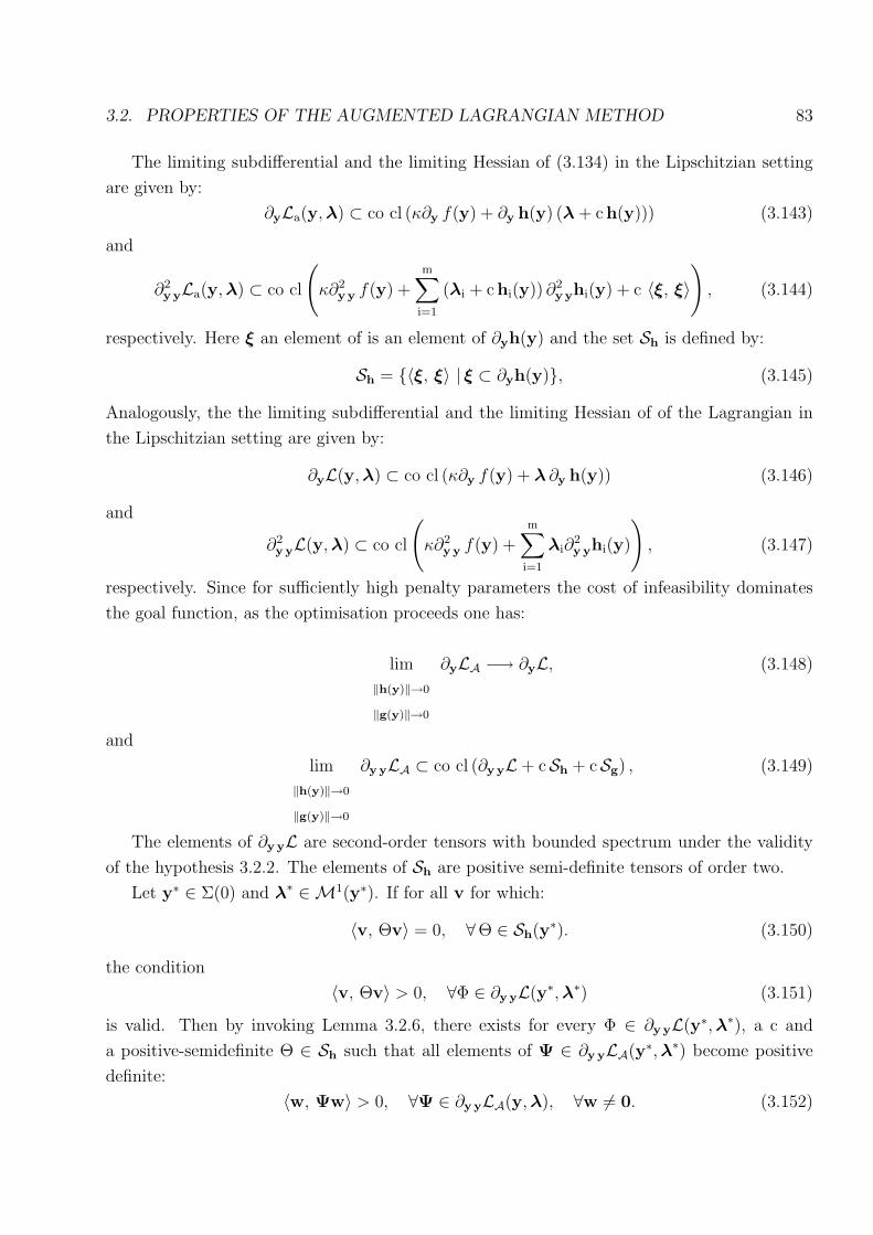
3.2. PROPERTIES OF THE AUGMENTED LAGRANGIAN METHOD 83
The limiting subdifferential and the limiting Hessian of (3.134) in the Lipschitzian setting
are given by:
∂yLa(y,λ) ⊂ co cl (κ∂y f(y) + ∂y h(y) (λ + ch(y))) (3.143)
and
∂2y yLa(y, λ) ⊂ co cl
(κ∂2
y y f(y) +m∑
i=1
(λi + chi(y)) ∂2y yhi(y) + c 〈ξ, ξ〉
), (3.144)
respectively. Here ξ an element of is an element of ∂yh(y) and the set Sh is defined by:
Sh = 〈ξ, ξ〉 | ξ ⊂ ∂yh(y), (3.145)
Analogously, the the limiting subdifferential and the limiting Hessian of of the Lagrangian in
the Lipschitzian setting are given by:
∂yL(y,λ) ⊂ co cl (κ∂y f(y) + λ ∂y h(y)) (3.146)
and
∂2y yL(y,λ) ⊂ co cl
(κ∂2
y y f(y) +m∑
i=1
λi∂2y yhi(y)
), (3.147)
respectively. Since for sufficiently high penalty parameters the cost of infeasibility dominates
the goal function, as the optimisation proceeds one has:
lim
‖h(y)‖→0
‖g(y)‖→0
∂yLA −→ ∂yL, (3.148)
and
lim
‖h(y)‖→0
‖g(y)‖→0
∂y yLA ⊂ co cl (∂yyL+ cSh + cSg) , (3.149)
The elements of ∂yyL are second-order tensors with bounded spectrum under the validity
of the hypothesis 3.2.2. The elements of Sh are positive semi-definite tensors of order two.
Let y∗ ∈ Σ(0) and λ∗ ∈M1(y∗). If for all v for which:
〈v, Θv〉 = 0, ∀Θ ∈ Sh(y∗). (3.150)
the condition
〈v, Θv〉 > 0, ∀Φ ∈ ∂yyL(y∗,λ∗) (3.151)
is valid. Then by invoking Lemma 3.2.6, there exists for every Φ ∈ ∂y yL(y∗,λ∗), a c and
a positive-semidefinite Θ ∈ Sh such that all elements of Ψ ∈ ∂y yLA(y∗,λ∗) become positive
definite:
〈w, Ψw〉 > 0, ∀Ψ ∈ ∂y yLA(y,λ), ∀w 6= 0. (3.152)

84 CHAPTER 3. NUMERICAL METHODS FOR FDLS
This gives the condition under which a local minimum of problem P , is convexified nonsmoothly
if it is characterised in terms of its augmented Lagrangian function. This result gives the
conditions when a nonconvex local minimum is convexified when the search directions are
projected to the tangent space Th=0(y) for some ε > 0 and ‖y∗ − y‖ ∈ B(y∗, ε).
3.2.5 Comparison of Strategies for the Solution of the Unconstrained
Minimisation
There are several aspects that make the augmented Lagrangian approach favorable in com-
parison to other approaches. In exact penalty methods, instead of performing a sequence of
minimisations, a single minimisation is performed but the penalty parameter has to be set very
high, such that ill-conditioning is caused, and depending on the minimisation method used
the condition number of the Hessian matrix is severed. The sequential minimisation besides
preventing ill-conditioning, allows partial minimisations especially at the initial stages of the
successive minimisations such that the successive minimisations proceed faster then expected.
The global optimizing property as in the exact penalty approach is however preserved. The
augmented Lagrangian is a method that is numerically compliant with the underlying penalty
approach. The Newton method in the minimisation of unconstrained functions is a favored
method because of its superlinear convergence in the vicinity of the solution. However, in large
scale optimisation problems where the structure of the Hessian matrix is not sparse, the eval-
uation of the Hessian matrix becomes cumbersome. In the case of the augmented Lagrangian
technique, in general, by the convexification induced by adding quadratic penalty terms to the
goal function, the structure of the Hessian matrix becomes dense. In such cases, quasi-Newton
methods are used in order to extrapolate the Hessian matrix by a formula like BFGS method.
If the function to be minimised is nonsmooth, then the nonuniqueness and unboundedness of
the Hessian may pose severe problems . A way to circumvent the problem of the nonunique-
ness and unboundedness of the Hessian matrix induced by using reformulation functions is
to use smoothing. This has the disadvantage however that the smoothing parameter has to
be adjusted in the course of the optimisation, which reduces the speed of the algorithm by
introducing additional loops in which the smoothing parameter is adjusted. The modified con-
jugate gradient methods offer a trade-off by performing a minimisation based on second-order
information without calculating them. The only required information is first-order informa-
tion such as the gradient and second-order information such that estimates of the Hessian are
extrapolated numerically, and it is not necessary to calculate the dense Hessian matrix. The
application of the augmented Lagrangian method to nonlinear programming problems with
equilibrium constraints is not wide spread. But the linear complementarity equality condition
is being linearised and relaxed first which introduces another burden except limiting the upper
value of the penalty factor. Below the main aspects in the comparison of different optimisation

3.2. PROPERTIES OF THE AUGMENTED LAGRANGIAN METHOD 85
approaches is presented:
1. One of the main advantages of direct-search methods is that the minimisation is performed
by function value comparison, so that the problems of ill-conditioning due to high penalty
parameters that degrade the performance of methods that use first and second-order
information, is not a problem for such methods.
2. The choice of a high penalty value has generally a convexifying effect so if the original
problem is not convex iterative first-order methods could face the dilemma of destabi-
lizing due to high c and divergence of low c. In this respect direct methods are more
suitable for a general class of optimisation problems. Direct search methods have the
disadvantage that their convergence in the vicinity of the solution is slow. A partial
remedy to this problem in the framework of the augmented Lagrangian technique is the
partial/incomplete minimisation approach in the intermediate stages of the successive
minimisations.
3. The local convexification of the feasible region, that is induced by the penalisation, guar-
antees that the unconstrained function is bounded-below and that through direct-search
methods the some feasible region is reached. Moreover, first-order methods can get stuck
in locally minimal solutions depending on severity of the nonconvexity of the value func-
tion and direct-search methods are less prone to such a problem.
4. Newton methods are preferred because of their fast convergence in the vicinity of the
solution. However, they are favorable in case of sparsity of the structure of the Hessian.
In general, for augmented Lagrangian functions the Hessian matrix is highly dense, which
impairs execution times for higher dimensional nonlinear programming problems .
5. Another issue for the Newton methods is the boundedness of the norm of the Hessian
matrix at the solution. Some reformulation functions, such as the Fischer-Burmeister
function, do not have bounded Hessians, and smoothing is necessary to implement those
together with Newton methods.
6. Sequential Quadratic Programming (SQP) relies on exploiting the resemblance of a smooth
nonlinear programming problem, to a standard Quadratic Programming (QP) problem.
The resemblance is achieved by successive linearisations of goal functions and constraints.
For nonsmooth functions these linearisations may provide less accurate approximations
at solution points.
7. In exact penalty methods, instead of performing a sequence of minimisations, a single
minimisation is performed but the penalty parameter has to be set very high, such that

86 CHAPTER 3. NUMERICAL METHODS FOR FDLS
ill-conditioning is caused, and depending on the minimisation method used the condition
number of the Hessian matrix is severed.
8. Bundle methods are commonly featuring in nonsmooth optimisation. They require in-
tensive information storage and processing of the subgradients, thus their efficiency and
computational speed is impaired by optimisation problems with more than 500 variables.
3.3 A NLP Scheme For The Calculation of Discontinu-
ous Optimal Trajectories for FDLS with Blockable
Degrees of Freedom
The sweeping discretisation method has been since its introduction in the late sixties been
investigated intensively as an integration routine. The aim is to investigate the properties of
the sweeping discretisation scheme from the point of optimisation, specifically from the point
of trajectory optimisation. The integration routines that are developed based on the sweeping
discretisation scheme are examined on the accuracy of the integration in literature. A partic-
ular interest is to determine switching times very accurately, at events such as opening of a
contact or stick-slip transitions at a contact. This is to exploit the quantitative properties of
the sweeping integration method as much as possible, but in the aspect of accuracy the event-
driven approaches excel the sweeping discretisation schemes. The advantage of using sweeping
discretisation in the trajectory optimisation problem is the qualitative advantages it offers with
respect to other optimisation approaches. By treating the contact forces and the forces that
induce transition as impulsive control and contact forces the distributional sense, one obtains in
some cases the mode sequence and optimal transition instants and locations in advance without
prespecifying them. The existence of switching control forces in the distributional sense, implies
that the transition indeed happen on a time-instant of Lebesgue measure zero if one considers
the continuous description of the problem, on the other side in the discretisation it means that
the transition happens on a discrete time interval on which the discretised differential mea-
sures of control forces exist in the distributional sense. The continuous description is compliant
to various hybrid system modeling approaches where transitions happen on a time instant of
Lebesgue-measure zero, whereas the discretised treatment the problem enables the transition
to take place on a time interval of length of the discretisation length. In literature there several
streams that treat in detail transitions on intervals with nonzero Lebesgue measure in order
to stay physical reality and deny conventional hybrid system descriptions by making use of
examples from the physical world. The measure-differential inclusion approach and the sweep-
ing discretisation comply in the continuous description with convential hybrid system modeling
approaches which are reasonable, whereas the discretised treatment accepts transitions on in-

3.3. NLP METHOD FOR MPEC 87
+
Upr( )Upr( )
gb
k+1
Nk
Nll
kNr
kN
k
Nll
kNr
k
gb
k+1
gbr
k+1
gbr
k+1g
br
k+1
gbl
k+1g
bl
k+1
gbl
k+1
Figure 3.4: The decomposition of the Upr relation into two unilateral primitives in
discretised form.
tervals. So by choosing minimum or maximum of discretisation step length it is possible to
limit transitions such that they comply with the physical system which is investigated. In the
opinion of the author, therefore it makes less sense to use sweeping discretisation if the aim
is to achieve numerical accuracy in the contact state transitions because of the existence of
contact forces in the distributional sense, and it recommends itself to revert to event-driven
integration schemes, whereas in order to obtain basically a robust treatment of a fairly complex
dynamical process sweeping discretisation scheme is superior in providing quantitative data on
the problem that compensates for the loss in the numerical accuracy. The high-level of numer-
ical accuracy is on the other hand unrealistic from the physical point of view most of the time.
One such superior advantage of sweeping integration techniques is the to provide statistically
accurate, experimentally verifiable information on granular flow consisting of many particles,
where the time evolution of singular particle is not relevant from the global view of the system.
By this approach modeling physical reality, the discretisation step length and its upper and
lower boundary has a physical significance. Choosing a discretisation step length which is much
smaller then any fast process that takes place in the real system under consideration does not
provide further information and may complicate the numerical execution.

88 CHAPTER 3. NUMERICAL METHODS FOR FDLS
Figure 3.5: The set-valued signum relation and its decomposition into two unilateral
primitives that represents relation between the discretised differential measure of normal
blocking force to the discretised differential measure of the control force in discretised form.

3.3. NLP METHOD FOR MPEC 89
3.3.1 The Transcription of a mechanical MDI Optimal Control Prob-
lem into a NLP
The problem is discretised in time over N equidistant points. The discretised form of the
measure-differential inclusion representation is stated in relations (2.120) to (2.123) are given
in relations (3.153) to (3.156):
M(qkm)
(uk+1 − uk
) − h(qkm,uk) ∆ t−B(qk
m)Γk = 0, k = 1, . . . N, (3.153)
−Γkbi
∈ Nki Sgn(γk+1
bi), ∀ i ∈ IB, k = 1, . . . N, (3.154)
|γk+1bi| ∈ Upr
(Nk
i
), ∀ i ∈ IB, k = 1, . . . N, (3.155)
τ k ∈ Cτ , k = 1, . . . N. (3.156)
The discretised differential measures of dΓbri , dΓbli , dNi, dΓbiare given by Γbri , Γbli , Ni, Γbi
.
These discretised differential measures exist in the distributional sense on a given discretisation
time interval. The position dependent entities in the discretised measure-differential inclusion
of the controlled mechanical system such as mass matrix M, vector h, B are evaluated at qm.
The force vector h is further evaluated at uk. The midpoint qkm is given by:
qkm = qk +
∆ t
2uk, (3.157)
and the discretisation in a time interval is given by:
qk+1m = qk
m +∆ t
2
(uk+1 + uk
). (3.158)
The representation of the set-valued control law stated in equations (3.154) and (3.155) in
discretised form is stated in relations (3.159) to (3.165) as a linear complementarity in the
given variables:
Γkbri
= Γkbi
+ Nki , k = 1, . . . N, ∀ i ∈ IB, (3.159)
Γkbli
= −Γkbi
+ Nki , k = 1, . . . N, ∀ i ∈ IB, (3.160)
γk+1bi
= γk+1bri
− γk+1bli
, k = 1, . . . N, ∀ i ∈ IB, (3.161)
γk+1bri
Γkbri
= 0, γk+1bri
≥ 0, Γkbri≥ 0, k = 1, . . . N, ∀ i ∈ IB, (3.162)
γk+1bli
Γkbli
= 0, γk+1bli
≥ 0, Γkbli≥ 0, k = 1, . . . N, ∀ i ∈ IB, (3.163)
γk+1bri
Nki = 0, γk+1
bri≥ 0, Nk
i ≥ 0, k = 1, . . . N, ∀ i ∈ IB, (3.164)
γk+1bli
Nki = 0, γk+1
bli≥ 0, Nk
i ≥ 0, k = 1, . . . N, ∀ i ∈ IB. (3.165)
The set valued relations which are stated in (3.154) and (3.155) are resolved by means of the
affine relations stated in equations (3.159) to (3.161) and by the mutual exclusivity conditions
stated in equations (3.162) to (3.165). The discretised forms of set-valued control laws depicted

90 CHAPTER 3. NUMERICAL METHODS FOR FDLS
in figures 2.10 and 2.6 can be seen in figures 3.4 and 3.5, respectively. The above discretisation
scheme is used for every DOF of the generalised coordinates. In the preparation of the numerical
method, the aim is to reduce the number of variables and constraints in order to decrease
execution time and inaccuracies in the numerical results. By making use of equalities given in
equations from (3.159) to (3.161) the variables Γkbri
, Γkbli
and γk+1bli
are eliminated. Further, by
making use of the affine relation between generalised position and velocities as given in equation
(3.158) the generalised positions are eliminated from the set of variables. More advanced
discretisation schemes may be found in the literature, such as the powerful Θ-method, an
algorithm based on displacements with proven convergence. The literature on the sweeping
based simulation of systems with friction and impacts is vast and a good overview is provided
in [7], [97], [98], [99], [100]. In order to achieve better efficiency from the optimisation algorithm
several steps are performed:
• By making use of the equalities stated in equations (3.159) to (3.161) variables are elim-
inated.
• All equality constraints that occur in the mathematical programming problem are trans-
formed into inequalities.
• By making use of the discretisation scheme in time, the generalised positions are expressed
in terms of generalised velocities and are eliminated as variables.
• The complementarities in (3.159) to (3.165) after preparation and elimination of some
variables are reformulated by the Fischer-Burmeister function.
For a scleronomic mechanical system with p blockable degrees of freedom, s-dimensional Lebesgue
measurable controls and f degrees of freedom, the nonlinear programming problem is set up.

3.3. NLP METHOD FOR MPEC 91
The optimal control problem in finite dimensional form is stated as below:
miny
f(y) k = 1, . . . N, (3.166)
Bk,j :f∑
l=1
mk,l(qkm, ω)(uk+1,l − uk,l)− h(qk
m, ω,uk)∆ t (3.167)
−p∑
l=1
wjl(q
km, ω)Γk
l −s∑
l=1
bjl(q
km, ω)τ k
l = 0, j = 1, . . . f,
RΦk,j : Φ(γk+1,jbr ,Γk,j + Nk,j) = 0, j = 1, . . . p, (3.168)
LΦk,j : Φ(γk+1,jbr − (wj(qk
m, ω))T uk+1, Nk,j − Γk,j) = 0, j = 1, . . . p, (3.169)
NRΦk,j : Φ(γk+1,jbr ,Nk,j) = 0, j = 1, . . . p, (3.170)
NLΦk,j : Φ(γk+1,jbr − (wj(qk
m, ω))T uk+1,Nk,j) = 0, j = 1, . . . p, (3.171)
τ k,jmin ≤ τ k,j ≤ τ k,j
max, j = 1, . . . s, (3.172)
Vj : qN+1j − qj
d = 0, j = 1, . . . f, (3.173)
Vj+f : uN+1j − uj
d = 0, j = 1, . . . f, (3.174)
tmin ≤ tf ≤ tmax. (3.175)
Here mk,l(qkm, ω) denotes the lth of the mass matrix M(qk
m, ω). The discretisation interval
is given by ∆ t = tfN. The vectors qd ∈ Rf , ud ∈ Rf denote the desired end states. The vectors
w(qkm, ω) and b(qk
m, ω) represent the generalised force directions of respective blocking forces
and the respective ordinary control forces, respectively. The variable vector y is composed of:
y =uk+1
1 , . . . ,uk+1f , τ k
1, . . . , τks ,Γ
kb1, . . . ,Γ
kbp, γ
k+1br,1 , . . . , γ
k+1br,p,N
k1, . . .N
kp, tf
,
k = 1, . . . , N. (3.176)
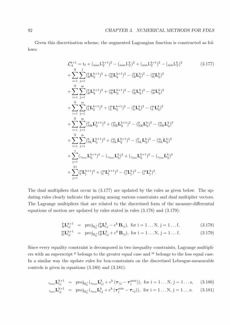
92 CHAPTER 3. NUMERICAL METHODS FOR FDLS
Given this discretisation scheme, the augmented Lagrangian function is constructed as fol-
lows:
Lk+1A = tf + (maxL
k+1T )2 − (maxL
kT)2 + (minL
k+1T )2 − (minL
kT)2 (3.177)
+N∑
i=1
f∑j=1
(pBLk+1
ij )2 + (mBLk+1
ij )2 − (pBLk
ij)2 − (m
BLkij)
2
+N∑
i=1
m∑j=1
(pRLk+1
ij )2 + (mRLk+1
ij )2 − (pRLk
ij)2 − (m
RLkij)
2
+N∑
i=1
m∑j=1
(pLL
k+1ij )2 + (m
L Lk+1ij )2 − (p
LLkij)
2 − (mL Lk
ij)2
+N∑
i=1
m∑j=1
(pNRLk+1
ij )2 + (mNRLk+1
ij )2 − (pNRLk
ij)2 − (m
NRLkij)
2
+N∑
i=1
m∑j=1
(pNLL
k+1ij )2 + (m
NLLk+1ij )2 − (p
NLLkij)
2 − (mNLL
kij)
2
+s∑
j=1
(τmaxLk+1ij )2 − (τmaxL
kij)
2 + (τminLk+1
ij )2 − (τminLk
ij)2
+2 f∑j=1
(pf L
k+1j )2 + (m
f Lk+1j )2 − (p
f Lkj )
2 − (mf Lk
j )2.
The dual multipliers that occur in (3.177) are updated by the rules as given below. The up-
dating rules clearly indicate the pairing among various constraints and dual multiplier vectors.
The Lagrange multipliers that are related to the discretised form of the measure-differential
equations of motion are updated by rules stated in rules (3.178) and (3.179):
pBLk+1
i,j = projR+0(pBLk
i,j − ck Bi,j), for i = 1 . . . N, j = 1 . . . f, (3.178)
mBLk+1
i,j = projR+0(mBLk
i,j + ck Bi,j), for i = 1 . . . N, j = 1 . . . f. (3.179)
Since every equality constraint is decomposed in two inequality constraints, Lagrange multipli-
ers with an superscript p belongs to the greater equal case and m belongs to the less equal case.
In a similar way the update rules for box-constraints on the discretised Lebesgue-measurable
controls is given in equations (3.180) and (3.181):
τmaxLk+1i,j = projR+
0(τmaxL
ki,j + ck (τ i,j − τmax
j )), for i = 1 . . . N, j = 1 . . . s, (3.180)
τminLk+1
i,j = projR+0(τmin
Lki,j + ck (τmin
j − τ i,j)), for i = 1 . . . N, j = 1 . . . s. (3.181)

3.3. NLP METHOD FOR MPEC 93
The Lagrange multipliers that belong to the boundary constraints and the bounds on final time
are are updated by the rules as stated in equations (3.182) to (3.185):
pf L
k+1j = projR+
0(pf L
kj − ck Vj), for j = 1 . . . 2 f, (3.182)
mf Lk+1
j = projR+0(mf Lk
j + ck Vj), for j = 1 . . . 2 f, (3.183)
maxLk+1T = projR+
0(maxL
kT + ck (tmin − tf)), (3.184)
minLk+1T = projR+
0(minL
kT + ck (tf − tmax)). (3.185)
The Lagrange multipliers that belong to the Fischer-Burmeister functions are updated by the
rules stated in equations (3.186) and (3.187):
pχL
k+1i,j = projR+
0(pχL
ki,j − ck
χΦi,j), for i = 1 . . . N, j = 1 . . . p, (3.186)
mχ Lk+1
i,j = projR+0(mχ Lk
i,j + ckχΦi,j), for i = 1 . . . N, j = 1 . . . p, (3.187)
for χ ∈ I = L, R, NL, NR.
3.3.2 Formulas for the Determination of the Numerical Gradient of
the Augmented Lagrangian
In order to implement the gradient based minimisation of the augmented Lagrangian as given
in equation (3.177) the gradient or set of gradients are analytically determined for the variables
given in (3.176).
Gradient of LkA with respect to ul,n
The gradient of the augmented Lagrangian with respect to all discretised generalised velocities
at every discretisation point and for every degrees of freedom is given by the expression (3.188):
∂ul,nLk
j =f∑
j=1
N∑i=1
(∂ul,n
Bi,j + ∂ql,iBi,j ∇ul,n
ql,i
) (pBLk+1
i,j − mBLk+1
i,j
)(3.188)
+
p∑j=1
N∑i=1
(∂ul,n
(LΦi,j) + ∂ql,i(LΦi,j) ∇ul,n
ql,i
)pLL
k+1i,j
−p∑
j=1
N∑i=1
(∂ul,n
(−LΦi,j) + ∂ql,i(−LΦi,j) ∇ul,n
ql,i
)mL Lk+1
i,j
+
p∑j=1
N∑i=1
(∂ul,n
(NLΦi,j) + ∂ql,i(NLΦi,j) ∇ul,n
ql,i
)pNLL
k+1i,j
−p∑
j=1
N∑i=1
(∂ul,n
(−NLΦi,j) + ∂ql,i(−NLΦi,j) ∇ul,n
ql,i
)mNLL
k+1i,j
+ ∂qlN+1
Vl ∇ul,nql
N+1
(mf Lk+1
l − pf L
k+1l
), n = 2 . . . N + 1, l = 1 . . . f.

94 CHAPTER 3. NUMERICAL METHODS FOR FDLS
Gradient of LkA with respect to final time tf
The gradient of the augmented Lagrangian with respect to the final time is given by the
expression (3.189):
∂tfLk =f∑
j=1
N∑i=1
(∂tfBi,j +
f∑
l=1
∂ql,iBi,j ∇tfql,i
)(pBLk+1
i,j − mBLk+1
i,j
)(3.189)
+
p∑j=1
N∑i=1
f∑
l=1
∂ql,i(LΦi,j) ∇tfql,i
pLL
k+1i,j − ∂ql,i
(−LΦi,j) ∇tfql,imL Lk+1
i,j
+
p∑j=1
N∑i=1
f∑
l=1
∂ql,i(NLΦi,j) ∇tfql,i
pNLL
k+1i,j − ∂ql,i
(−NLΦi,j) ∇tfql,imNLL
k+1i,j
+f∑
j=1
∂qjN+1
(Vj) ∇tfqjN+1
(mf Lk+1
j − pf L
k+1j
).
Gradient of LkA with respect to discretised Lebesgue-measurable controls τi,l
The gradient of the augmented Lagrangian with respect to the Lebesgue measurable controls
τi,l at every discretisation point and for every controls is given by the expression (3.190):
∂τi,lLk =f∑
j=1
∂τi,lBi,j
(pBLk+1
i,j − mBLk+1
i,j
)+ (τmin
Lki,l − τmaxL
ki,l), (3.190)
l = 1 . . . s, i = 1 . . . N.
Gradient of LkA with respect to the discretised differential measure of blocking
controls Γi,l
The gradient of the augmented Lagrangian with respect to the discretised differential-measure
of the blocking controls Γi,l at every discretisation interval and for every blocking controls is
given by the expression (3.191):
∂Γi,lLk =
f∑j=1
∂Γi,lBi,j
(pBLk+1
i,j − mBLk+1
i,j
)(3.191)
+
p∑j=1
∂Γi,l(LΦi,j)
pLL
k+1i,j − ∂Γi,l
(−LΦi,j)mL Lk+1
i,j + ∂Γi,l(RΦi,j)
pRLk+1
i,j − ∂Γi,l(−RΦi,j)
mRLk+1
i,j
l = 1 . . . p, i = 1 . . . N.

3.3. NLP METHOD FOR MPEC 95
Gradient of LkA with respect to the discretised differential measure of controls Ni,l
The gradient of the augmented Lagrangian with respect to the discretised differential-measure
of the blocking controls Ni,l at every discretisation interval and for every blocking controls is
given by the expression (3.192):
∂Ni,lLk =
∑
∀χ∈I
p∑j=1
∂Ni,l(χΦi,j)
pχL
k+1i,j − ∂Ni,l
(−χΦi,j)mχ Lk+1
i,j , l = 1 . . . p i = 1 . . . N (3.192)
for χ ∈ I = L, R, NL, NR.
Gradient of LkA with respect to the γ i+1
br,l
The gradient of the augmented Lagrangian with respect to the discretised slack velocity γ i+1br,r,l
at every discretisation point and for every blockable direction is given by the expression (3.193):
∂γi+1br,lLk =
∑
∀χ∈I
p∑j=1
∂γi+1br,l
(χΦi,j)pχL
k+1i,j − ∂γi+1
br,l(−χΦi,j)
mχ Lk+1
i,j , l = 1 . . . p, i = 1 . . . N (3.193)
for χ ∈ I = L, R, NL, NR.
3.3.3 An Augmented Lagrangian Based Nonlinear Programming Al-
gorithm
The algorithm consists of three loops which are embedded in each other as shown in figure 3.6.
The most outer iteration which is the main iteration is controlling the level of nonlinearity of
the system. The continuation parameter ω is screwed slowly upwards so that when ω becomes
one the system of equalities and inequalities represents the discretised mechanical system,
and if ω is zero the system resembles a linear mechanical system. The intermediate iteration
performs for each given ω a number of successive minimisations of the resulting augmented
Lagrangian functional Lka and updates after every minimisation the Lagrange multiplier vectors
L according to relations from (3.178) to (3.187). The inner iteration performs the minimisation
of the augmented Lagrangian Lka at stage k for a given ω and Lagrange multiplier vector Lk
by a modified conjugate gradients method as shown in flowchart 3.7. The formulas for the
augmented Lagrangian functional, update of Lagrange multipliers and the subgradient of the
augmented Lagrangian are given in the preceding section.
The conjugate gradient algorithm does not use prespecified conjugate directions, but instead
computes the directions as the algorithm progresses. At each stage of the algorithm, the
direction is calculated as a linear combination of the previous direction and the current gradient,
in a such a way that all the directions are mutually Q-conjugate. This method makes use of
the fact that for a quadratic function of n variables, one can locate the function minimizer
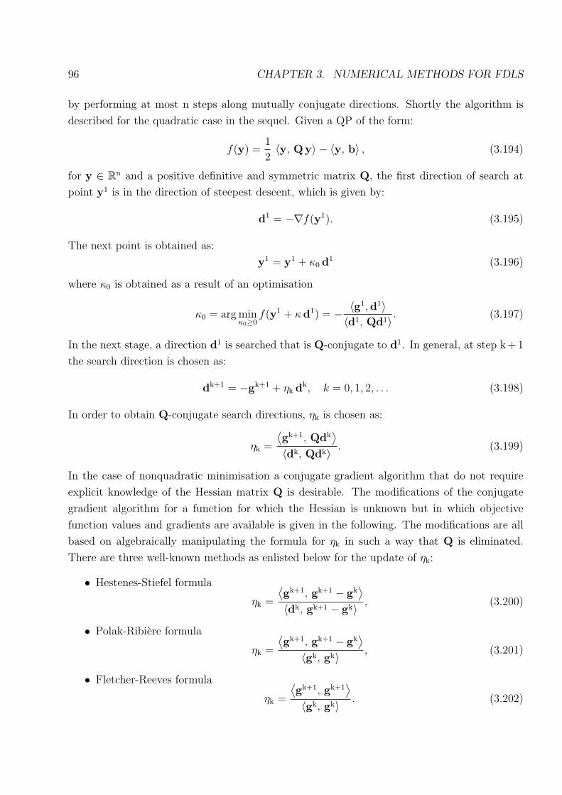
96 CHAPTER 3. NUMERICAL METHODS FOR FDLS
by performing at most n steps along mutually conjugate directions. Shortly the algorithm is
described for the quadratic case in the sequel. Given a QP of the form:
f(y) =1
2〈y, Qy〉 − 〈y, b〉 , (3.194)
for y ∈ Rn and a positive definitive and symmetric matrix Q, the first direction of search at
point y1 is in the direction of steepest descent, which is given by:
d1 = −∇f(y1). (3.195)
The next point is obtained as:
y1 = y1 + κ0 d1 (3.196)
where κ0 is obtained as a result of an optimisation
κ0 = arg minκ0≥0
f(y1 + κd1) = − 〈g1,d1〉〈d1, Qd1〉 . (3.197)
In the next stage, a direction d1 is searched that is Q-conjugate to d1. In general, at step k+1
the search direction is chosen as:
dk+1 = −gk+1 + ηk dk, k = 0, 1, 2, . . . (3.198)
In order to obtain Q-conjugate search directions, ηk is chosen as:
ηk =
⟨gk+1, Qdk
⟩
〈dk, Qdk〉 . (3.199)
In the case of nonquadratic minimisation a conjugate gradient algorithm that do not require
explicit knowledge of the Hessian matrix Q is desirable. The modifications of the conjugate
gradient algorithm for a function for which the Hessian is unknown but in which objective
function values and gradients are available is given in the following. The modifications are all
based on algebraically manipulating the formula for ηk in such a way that Q is eliminated.
There are three well-known methods as enlisted below for the update of ηk:
• Hestenes-Stiefel formula
ηk =
⟨gk+1, gk+1 − gk
⟩
〈dk, gk+1 − gk〉 , (3.200)
• Polak-Ribiere formula
ηk =
⟨gk+1, gk+1 − gk
⟩
〈gk, gk〉 , (3.201)
• Fletcher-Reeves formula
ηk =
⟨gk+1, gk+1
⟩
〈gk, gk〉 . (3.202)

3.3. NLP METHOD FOR MPEC 97
Figure 3.6: The simplified flowchart of the algorithm.
These modified conjugate gradient strategies rely on estimating the Hessian of a nonquadratic
goal function and requires updating of the search direction to the exact gradient every certain
number of steps. It is not clear which of these methods is superior since their performance is
quite problem specific. In the case where the Hessian is not determined explicitly, the optimal
value of κ can not be given in a closed form as in equation (3.197). The step given in equation
(3.196) is replaced by a line search algorithm. The line search method in determining the
minimum in the direction of search has been an interpolation based on bisection line search.
The termination criteria for the intermediate iterations take advantage of a property of
the augmented Lagrangian method which is called partial minimisation. The minimisations
between successive Lagrange multiplier updates is not performed exactly but instead partially
so that the slow convergence in the vicinity of the intermediate minima does not pose a severe
problem to the run times. The number of minimisations performed for each value of ω are
increased linearly proportional as it approaches one. The number of steps for the minimisation
of each augmented Lagrangian is also increased to the square of the corresponding ω-stage.
The primal variables of the optimisation have been inherited to the next ω-stage. The dual
values are also inherited to the next stage except at initial stages of the optimisation.

98 CHAPTER 3. NUMERICAL METHODS FOR FDLS
Figure 3.7: The flowchart of the conjugate gradients minimisation.

3.4. NUMERICAL EXAMPLE 99
3.3.4 Implementation of the Algorithm
The algorithm has been implemented with MATLAB. The numerically intensive and time
consuming parts has been programmed in C and by the generation of mex-files, these C codes
are appended to the MATLAB main routine. The ANSI C codes have reduced the run times
extensively. Following tasks in the optimisation have been performed with mex-files:
• The function evaluations of the augmented Lagrangian La,
• The interpolations base on bisection line search,
• The update of Lagrange multipliers,
• The evaluation of the exact gradient of the augmented Lagrangian function,
• The conjugate gradients minimisation of the augmented Lagrangian function.
The programming approach based on combining MATLAB and ANSI C codes provides flexi-
bility to perform modifications easily whereas the runtimes are drastically reduced by codes.
In the design of the structure of the code modularity has been a prime issue in order to
enable easy adaptation of the code to other optimisation problems. This has been achieved by
characterizing each optimisation by its unique gradient and augmented Lagrangian function.
Easy interchangeablity of gradient and augmented Lagrangian modules are achieved.
3.4 Numerical Example
In this section a numerical example for the algorithm that is explained in section 3.3 is presented.
The investigated mechanical system is shown in figure 3.8. It has two rotational degrees of
freedom denoted by α and β. The DOF α is measured in the positive sense from the Iex axis
of the inertial frame I, which is located at the point O. The DOF is β is measured in the
positive sense from the Iex axis of the inertial frame I as shown in figure 3.8. The link 1 rotates
around point O and link 2 rotates around point A which is attached to link 1. The motor at
link O drives the system by the Lebesgue measurable control force τ , which has upper and
lower limits denoted by τmin and τmax, respectively. The brake at A connected to the links one
and two, has two operating modes, either it allows totally free motion or it blocks such that
the relative angular velocity between links one and two given by α− β reduces immediately to
zero. This requires depending on the pre-blocking state of the system a jump in the relative
angular velocity, which only can be induced by impulsive forces. The center of masses of the
links 1 and 2 are denoted by S1 and S2, respectively. The moments of inertia of links 1 and 2
with respect to the their center of masses are given by Θ1 and Θ2, respectively. The masses
of the links are denoted by m1 and m2, respectively and the lengths of each link is given by l1

100 CHAPTER 3. NUMERICAL METHODS FOR FDLS
ex
ey
a
m l1
Q11
m l2
Q2 2
O
S1
bI
I
d1
d2
S2
m4
Q4
m3
Q3
A
Figure 3.8: The parameters of the planar double pendulum.
and l2. The center of mass of the brake is located at A and the mass and moment of inertia of
the brake with respect to A are given by m4 and Θ4, respectively. Similarly, the motor, that is
located at O has mass m3 and moment of inertia Θ3 with respect to O. The numerical values
d1 and d2 denote the distances ‖O S1‖ and ‖AS2‖, respectively. The system consists of two
rigid bodies. The first rigid body consists of link one, the motor, and the part of the brake that
moves with link one. The second rigid body consists of link two and the part of the brake that
moves together with link two. Accordingly, the physical properties of mass and inertia of the
rigid bodies one and two, as well as positions of the respective center of masses rcm1 and rcm2
depend on the physical properties of the constituent components. With respect to the number
of degrees of freedom, the system has two operating modes. If the brake does not block, the
system is a double pendulum in the plane, and if the brake hinders relative motion of the second
link with respect to the first link then the system has one rotational degree of freedom. Indeed,
the system has infinitely many modes in the one degree of freedom case depending at which
relative degree α − β the underactuated link is kept blocked. In the sequel, two time-optimal
trajectories are investigated and presented. Since blocking is an highly dissipative process as
presented in subsection 2.6.3, it is suitable in the context of time-optimal control then any other
goal function such as control-effort optimal control. The numerical values of various parameters
in numerical case study is given in table 3.1. The equality and inequality constraints of the

3.4. NUMERICAL EXAMPLE 101
m1 m2 m3 m4 Θ1 Θ2 Θ3 Θ4 l1 l2 |τ |[kg] [kg] [kg] [kg] [kg m2] [kg m2] [kg m2] [kg m2] [m] [m] [nm]
1 1 1 1 0.05 0.05 0.05 0.05 1 1 < |2|m41 m42 d1 d2 m1 m2 m3 V1 V2 rcm1 rcm2
[kg] [kg] [m] [m] [kg m2] [kg m2] [kg m2] [−] [−] [m] [m]
0.5 0.5 l12
l22
1.16 19
13
0.2755 2.069 0.4 13
Table 3.1: System parameters of the manipulator for cases A, B, C.
Inequality Dual Multiplier Inequality Dual Multiplier
ΦR ¹ 0 pLR −ΦR ¹ 0 mLR
ΦL ¹ 0 pLL −ΦL ¹ 0 mLL
ΦNL ¹ 0 pLNL −ΦNL ¹ 0 mLNL
ΦNR ¹ 0 pLNR −ΦNR ¹ 0 mLNR
Bα ¹ 0 pBLα −Bα ¹ 0 m
BLα
Bβ ¹ 0 pBLβ −Bβ ¹ 0 m
BLβ
τ − τmax ¹ 0 maxLτ τmin − τ ¹ 0 minLτ
βN+1 − βf ≤ 0 pLβf βf − βN+1 ≤ 0 mLβf
αN+1 − αf ≤ 0 pLαf αf − αN+1 ≤ 0 mLαf
βN+1 − βf ≤ 0 pLβf βf − βN+1 ≤ 0 mLβf
αN+1 − αf ≤ 0 pLαf αf − αN+1 ≤ 0 mLαf
tf − tmax ≤ 0 maxLtf tmin − tf ≤ 0 minLtf
Table 3.2: Correspondence between inequalities and dual multipliers in the NLP of the
planar double pendulum.

102 CHAPTER 3. NUMERICAL METHODS FOR FDLS
NLP are given below for k = 1 . . . N, in relations (3.203) to (3.216):
(α[k + 1] − α[k]) + ω V1 cos(αm[k]− βm[k])(β[k + 1]− β[k]) (3.203)
+ω V1 ∆t sin(αm[k]− βm[k]) β2[k]− τ [k] ∆t + Γ[k] = 0,
(β[k + 1] − β[k]) + ω V2 cos(αm[k]− βm[k])(α[k + 1]− α[k]) (3.204)
−ω V2 ∆t sin(αm[k]− βm[k]) α2[k]− Γ[k] = 0,
ΦFB ((Γ[k] + N[k]), γbr[k + 1]) = 0, (3.205)
ΦFB ((−Γ[k] + N[k]),γbr[k + 1] + α[k + 1]− β[k + 1]) = 0, (3.206)
ΦFB (γbr[k + 1],N[k]) = 0, (3.207)
ΦFB (γbr[k + 1] + α[k + 1]− β[k + 1],N[k]) = 0, (3.208)
τ [k]− τmax ≤ 0, (3.209)
τmax − τ [k] ≤ 0, (3.210)
tf − tmax ≤ 0, (3.211)
tmin − tf ≤ 0, (3.212)
α[N + 1]− αf = 0, (3.213)
β[N + 1]− βf = 0, (3.214)
α[N + 1]− αf = 0, (3.215)
β[N + 1]− βf = 0. (3.216)
In the sequel equations (3.203) and (3.204) are denoted by Bα[k] and Bβ[k], respectively. The
corresponding dual multipliers are shown in table 3.2. The center of masses, equivalent inertias
and some other parameters are formulated in dependence on the physical properties of the
constituent components as below:
rcm1 = l1(m1
2+ m41)
m41 + m1 + m3
,
rcm2 = m2l2
2 (m42 + m2),
Θcm1 = Θ1 + Θ3 + Θ41 + m1 (l12− rcm1)
2 + m3 r2cm1 + m41 (l1 − rcm1)
2,
Θcm2 = Θ42 + Θ2 + m2 (l22− rcm2)
2 + m42 r2cm2,
m1 = m1 r2cm1 + m2 l21,
m2 = m2 r2cm2,
m3 = m2 l1 rcm2,
V1 =m3
m1 + Θ1
,
V2 =m3
m2 + Θ2
.

3.4. NUMERICAL EXAMPLE 103
3.4.1 Case A
In this maneuver the aim is to reach the final position given by αf = 3 π4
, βf = π, αf = 0, βf = 0
time-optimally.
The numerical information on the maneuver A is given in table 3.4. The problem is dis-
cretized over a number of 201 points. In this time-optimal maneuver the system starts in the
blocked state. The whole maneuver takes 3.395 seconds. There are eight transitions at times
t[27] = 0.46 s, t[34] = 0.58 s, t[89] = 1.51 s, t[158] = 2.68 s, t[159] = 2.7 s, t[199] = 3.38 s. At
t[27] the underactuated link is released. At transition interval P[34], the underactuated link is
blocked impactively. The relative velocity γbr[34] is decreased by 1.60 radsec
to −2.3927 · 10−4 radsec
.
The discretised differential measure of the normal control force N[34] that is applied in P[34]
is 18.98 N m sec and impulsive control force that is applied to brake down the passive link
amounts to Γ[34] = 10.88 N m sec. The passive link is again released at t[89] = 1.51 s, and is
impactively blocked during interval P[158] by N[158] = 34.50 N m sec and impulsive control
force that amounts to Γ[158] = −34.50 N m sec. The relative velocity γbr[158] is increased by
0.34 radsec
to γbr[159] = −1.5094 · 10−3 radsec
. At transition time t[159] = 2.7 s the passive link
is released and is impactively blocked during interval P[199] by N[199] = 37.95 N m sec and
impulsive control force that amounts to Γ[199] = 37.96 N m sec. The relative velocity γbr[199]
is decreased by 3.31 radsec
to γbr[200] = 0.0035 radsec
. The mode sequence and the duration of each
mode is given in table 3.3. The action of the double pendulum is seen in figure 3.10. Quali-
tatively, the motor accelerates the system in the blocked phase and throws the underactuated
link at t[89] = 1.51 s, by releasing the second link, and switching to maximal deceleration, in
order to increase the relative angle as fast as possible. This serves two goals; namely; it reduces
the equivalent moment of inertia that resists the motor in moving the system to the desired
end state, and brings the second link closer to the desired relative angle of 135 degrees. The
motor accelerates the system again. The final stage of the maneuver starts with the impulsive
blocking and releasing action at t[158] = 2.68 s during interval P[158]. The relative angle over-
shoots 135 degrees, and the system this by making use of the dynamic coupling between the
actuated and underactuated link. The impulsive blocking at t[158] = 2.68 s serves to stop the
overshooting motion by reducing the relative velocity and acceleration to zero as can be seen in
figures 3.9 and 3.10. Figure 3.11 depicts the evolution of the optimal motor-torque history and
the discretised measures of normal contact force and frictional braking moment. Figure 3.12
depicts the numerical residues of equations Bα[k]∆t
andBβ [k]
∆t, respectively. The residues indicate
the level of accuracy which is attained at the solution. Figure 3.13 presents the residues of the
four reformulation functions. The actual values of the complementarities are shown in figure
3.18. The dual multipliers for various inequalities as listed in table 3.3 are listed in figures 3.14,
3.16 and 3.17. The evolution of the costate dynamics has been obtained by a post optimisation
calculation and are shown in figure 3.15.

104 CHAPTER 3. NUMERICAL METHODS FOR FDLS
Figure 3.9: Case A: The optimal evolution of the generalised velocities α, β, relative
velocity α− β, generalize positions α, β and relative position α− β. ( red lines mark the
transition times)

3.4. NUMERICAL EXAMPLE 105
Modes 1-DOF 2-DOF 1-DOF 2-DOF 1-DOF 2-DOF 1-DOF
Duration 0.458 s 0.12 s 0.93 s 1.17 s 0.017 s 0.68 s 0.017 s
Intervals 1-27 27-34 34-89 89-158 158-159 159-199 199-200
Table 3.3: Case A: The mode sequence, duration and intervals of modes.
] of disc. points 200 penalty c 1e5 ] of primal variables 1201
] of dual variables 2810 increment in ω 0.1 kstage 40
] of complementarities 800 α0 [rad] 0 α0 [rad/sec] 0
αf [rad] 3 π4
αf [rad/sec] 0 β0 [rad] 0
β0 [rad/sec] 0 βf [rad] π βf [rad/sec] 0
Table 3.4: Case A: Optimisation parameters, initial and final states of the optimisation.
0.46 s 0.58s1.51 s2.68 s
3.38 s
Figure 3.10: Case A: Maneuver of the double pendulum (Color code: For link 2 white is
blocked, black is unblocked, for link 1 green position at transition interval).
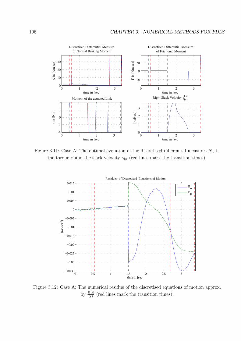
106 CHAPTER 3. NUMERICAL METHODS FOR FDLS
Figure 3.11: Case A: The optimal evolution of the discretised differential measures N , Γ,
the torque τ and the slack velocity γbr (red lines mark the transition times).
0 0.5 1 1.5 2 2.5 3−0.035
−0.03
−0.025
−0.02
−0.015
−0.01
−0.005
0
0.005
0.01
0.015
Residues of Discretised Equations of Motion
[rad
/sec
2 ]
time in [sec]
BαBβ
Figure 3.12: Case A: The numerical residue of the discretised equations of motion approx.
by B[k]∆ t
(red lines mark the transition times).

3.4. NUMERICAL EXAMPLE 107
0 0.5 1 1.5 2 2.5 3−8
−6
−4
−2
0
x 10−3 Residue of Φ
R
time in [sec]0 0.5 1 1.5 2 2.5 3
0
1
2
3
4x 10
−3 Residue of ΦL
time in [sec]
0 0.5 1 1.5 2 2.5 3−8
−6
−4
−2
0
x 10−3 Residue of Φ
NR
time in [sec]0 0.5 1 1.5 2 2.5 3
−2
0
2
4x 10
−3 Residue of ΦNL
time in [sec]
Figure 3.13: Case A: Residues of the reformulation functions ΦR, ΦL, ΦNR and ΦNL (red
lines mark the transition times).
0 1 2 30
200
400
600
mB
Lα
time in [sec]0 1 2 3
0
200
400
600
800
mB
Lβ
time in [sec]
0 1 2 30
500
1000
1500
pB
Lα
time in [sec]0 1 2 3
0
500
1000
pB
Lβ
time in [sec]
Figure 3.14: Case A: The optimal evolution of the dual multipliers mBLα, m
BLβ, pBLα and p
BLβ
(red lines mark the transition times).

108 CHAPTER 3. NUMERICAL METHODS FOR FDLS
0 1 2 3
−1000
−500
0
500
Lα
time in [sec]0 1 2 3
−1000
−500
0
500
Lβ
time in [sec]
Figure 3.15: Case A: The time evolution of the costate dynamics in the second-order form
(red lines mark the transition times).
0 1 2 30
1000
2000
3000
4000
m LR
time in [sec]0 1 2 3
0
5000
10000
m LL
time in [sec]
0 1 2 30
1
2
x 104
p LR
time in [sec]0 1 2 3
0
100
200
p LL
time in [sec]
Figure 3.16: Case A:The optimal evolution of the dual multipliers mLR, mLL, pLR and pLL
(red lines mark the transition times).
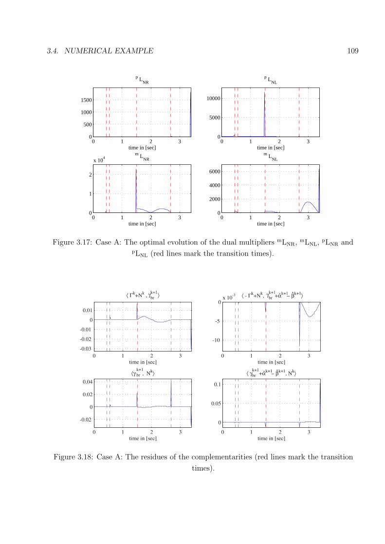
3.4. NUMERICAL EXAMPLE 109
0 1 2 30
500
1000
1500
p LNR
time in [sec]0 1 2 3
0
5000
10000
p LNL
time in [sec]
0 1 2 30
1
2
x 104
m LNR
time in [sec]0 1 2 3
0
2000
4000
6000
m LNL
time in [sec]
Figure 3.17: Case A: The optimal evolution of the dual multipliers mLNR, mLNL, pLNR andpLNL (red lines mark the transition times).
Figure 3.18: Case A: The residues of the complementarities (red lines mark the transition
times).

110 CHAPTER 3. NUMERICAL METHODS FOR FDLS
Modes 1-DOF 2-DOF 1-DOF 2-DOF 1-DOF
Duration 0.41 s 0.68 s 0.75 s 0.57 s 2.11 s
Intervals 1-19 19-49 49-82 82-107 107-200
Table 3.5: Case B: The mode sequence, duration and intervals of modes.
3.4.2 Case B
In this maneuver the aim is to reach the final position given by αf = π, βf = π, αf = 0,
βf = 0 time-optimally. The numerical information on the maneuver B is given in table 3.6.
The problem is discretized over a number of 201 points. In this time-optimal maneuver the
system starts in the blocked state. The whole maneuver takes 4.53 seconds. There are four
transitions at times t[19] = 0.43 s, t[49] = 1.11 s, t[82] = 1.86 s, t[107] = 2.42 s. At t[19]
the underactuated link is released. At transition interval P[49], the underactuated link is
blocked impactively. The relative velocity γbr[49] is decreased by 2.41 radsec
to 3.6776 · 10−4 radsec
.
The discretised differential measure of the normal control force N[49] that is applied in P[49]
is 62.00 N m sec and impulsive control force that is applied to brake down the passive link
amounts to Γ[49] = 61.97 N m sec. The passive link is again released at t[82] = 1.86 s, and is
impactively blocked during interval P[107] by N[107] = −34.88 N m sec and impulsive control
force that amounts to Γ[107] = −34.65 N m sec. The relative velocity γbr[107] is increased
by 7.55 radsec
to γbr[107] = −6.0490 · 10−4 radsec
. The mode sequence and the duration of each
mode is given in table 3.5. The maneuver of the underactuated manipulator is seen in figure
3.20. Qualitatively, the motor accelerates the system with unblocked underactuated link. The
relative angle decreases such that the equivalent moment of inertia, that resists the motor is
reduced. The link two is then kept blocked between 1.11 s and 1.86 s. The release of link
two enables to throw it to the desired final position. As the desired relative angle of 0 degrees
is reached, the arm is blocked impulsively, and the motor decelerates the system to the final
position in a bang-bang manner.
Figure 3.21 depicts the evolution of the optimal motor-torque history and the discretised
measures of normal contact force and frictional braking moment. Figure 3.22 depicts the
numerical residues of equations Bα[k]∆t
andBβ [k]
∆t, respectively. The residues indicate the level
of accuracy which is attained at the solution. Figure 3.23 presents the residues of the four
reformulation functions. The actual values of the complementarities are shown in figure 3.28.
The dual multipliers for various inequalities as listed in table 3.3 are listed in figures 3.24, 3.26
and 3.27. The evolution of the costate dynamics has been obtained by a post optimisation
calculation and are shown in figure 3.25.

3.4. NUMERICAL EXAMPLE 111
] of disc. points 200 penalty c 1e5 ] of primal variables 1201
] of dual variables 2810 increment in ω 0.1 kstage 40
] of complementarities 800 α0 [rad] 0 α0 [rad/sec] 0
αf [rad] π αf [rad/sec] 0 β0 [rad] 0
β0 [rad/sec] 0 βf [rad] π βf [rad/sec] 0
Table 3.6: Case B: Optimisation parameters, initial and final states of the optimisation.
Figure 3.19: Case B: The optimal evolution of the generalised velocities α, β, relative
velocity α− β, generalised positions α, β and relative position α− β. red lines mark the
transition times)

112 CHAPTER 3. NUMERICAL METHODS FOR FDLS
chattering
2.42 s
1.86 s1.11 s
0.43 s
Figure 3.20: Case B: Maneuver of the double pendulum (Color code: For link 2 white is
blocked, black is unblocked, for link 1 green position at transition interval).
Figure 3.21: Case B: The optimal evolution of the discretised differential measures N , Γ,
the torque τ and the slack velocity γbr (red lines mark the transition times).

3.4. NUMERICAL EXAMPLE 113
0 0.5 1 1.5 2 2.5 3 3.5 4 4.5
−0.01
−0.005
0
0.005
0.01
Residues of Discretised Equations of Motion
[rad
/sec
2 ]
time in [sec]
BαBβ
Figure 3.22: Case B: The numerical residue of the discretised equations of motion of motion
approx. by B[k]∆ t
(red lines mark the transition times).
0 1 2 3 4
−10
−5
0
x 10−4 Residue of Φ
R
time in [sec]0 1 2 3 4
0
2
4
6
8
x 10−3 Residue of Φ
L
time in [sec]
0 1 2 3 4
−0.03
−0.02
−0.01
0
Residue of ΦNR
time in [sec]0 1 2 3 4
0
2
4
6
8
x 10−3 Residue of Φ
NL
time in [sec]
Figure 3.23: Case B: Residues of the reformulation functions ΦR, ΦL, ΦNR and ΦNL (red
lines mark the transition times).

114 CHAPTER 3. NUMERICAL METHODS FOR FDLS
0 1 2 3 40
200
400
600
800
mB
Lα
time in [sec]0 1 2 3 4
0
500
1000
mB
Lβ
time in [sec]
0 1 2 3 40
500
1000
pB
Lα
time in [sec]0 1 2 3 4
0
500
1000
pB
Lβ
time in [sec]
Figure 3.24: Case B: The optimal evolution of the dual multipliers mBLα, m
BLβ, pBLα and p
BLβ
(red lines mark the transition times).
0 1 2 3 4
−1000
−500
0
500
Lα
time in [sec]0 1 2 3 4
−500
0
500
Lβ
time in [sec]
Figure 3.25: Case B: The time evolution of the costate dynamics in the second-order form
(red lines mark the transition times).

3.4. NUMERICAL EXAMPLE 115
0 1 2 3 40
200
400
600
800
m LR
time in [sec]0 1 2 3 4
0
1
2
3
x 104
m LL
time in [sec]
0 1 2 3 40
1000
2000
3000
4000
p LR
time in [sec]0 1 2 3 4
0
500
1000
1500
p LL
time in [sec]
Figure 3.26: Case B:The optimal evolution of the dual multipliers mLR, mLL, pLR and pLL
(red lines mark the transition times).
0 1 2 3 40
500
1000
p LNR
time in [sec]0 1 2 3 4
0
1
2
3
4x 10
4p L
NL
time in [sec]
0 1 2 3 40
5
10
x 104
m LNR
time in [sec]0 1 2 3 4
0
2000
4000
m LNL
time in [sec]
Figure 3.27: Case B:The optimal evolution of the dual multipliers mLNR, mLNL, pLNR andpLNL (red lines mark the transition times).

116 CHAPTER 3. NUMERICAL METHODS FOR FDLS
Figure 3.28: Case B: The residues of the complementarities (red lines mark the transition
times).
3.4.3 Case C
In this maneuver the aim is to reach the final position given by αf = π, βf = π, αf = 0, βf = 0
time-optimally. The numerical parameters used in the optimisation are seen in table 3.8. In this
time-optimal maneuver the system starts in the blocked state. The whole maneuver takes 2.77
seconds. There are four transitions at times t[3] = 0.04155 s, t[96] = 1.3296 s, t[147] = 2.036 s,
t[187] = 2.59 s. At t[3] the underactuated link is released. At transition interval P[96], the
underactuated link is blocked impactively. The relative velocity γbr[96] is reduced by 0.5 radsec
to −0.0225 radsec
. The discretized differential measure of the normal control force N[96] that
is applied in P[96] is 38.64 N m sec and impulsive control force that is applied to brake down
the passive link amounts to Γ[96] = −38.64 N m sec. The passive link is again released at
t[147] = 2.036 s, and is impactively blocked during interval P[187] by N[187] = 73.71 N m sec
and impulsive control force that amounts to Γ[187] = 73.71 N m sec. The relative velocity
γbr[187] is reduced by 2.0262 radsec
to γbr[188] = 0.0022 radsec
. The mode sequence and the duration
of each mode is given in table 3.7. Qualitatively, the maneuver can be divided into three parts.
In the first part of the maneuver, the motor moves the first link in clockwise direction while
the second link is unblocked. The relative angle is decreased as seen in figure 3.29, and the
underactuated link is blocked at 1.32 seconds. The aim of the maneuver, is to block the second
arm in a position so that the equivalent moment of inertia that resists the motor is minimised.
In the second part of the maneuver, the motor rushes to the position α = π2
while the second

3.4. NUMERICAL EXAMPLE 117
Modes 1-DOF 2-DOF 1-DOF 2-DOF 1-DOF
Duration 0.04 s 1.29 s 0.71 s 0.55 s 0.18 s
Intervals 1-3 3-96 96-147 147-187 187-200
Table 3.7: Case C: The mode sequence, duration and intervals of modes.
] of disc. points 200 penalty c 1e5 ] of primal variables 1201
] of dual variables 2810 increment in ω 0.1 kstage 40
] of complementarities 800 α0 [rad] 0 α0 [rad/sec] 0
αf [rad] π2
αf [rad/sec] 0 β0 [rad] 0
β0 [rad/sec] 0 βf [rad] π βf [rad/sec]
Table 3.8: Case C: Optimisation parameters, initial and final states of the optimisation.
link is blocked until 2.04 seconds. At this time instant, the underactuated link is released so
that through the dynamic coupling. it moves to the end position β = π, where it is impactively
blocked at the final time instant at 2.59 seconds.
Figure 3.31 depicts the evolution of the optimal motor-torque history and the discretised
measures of normal contact force and frictional braking moment. Figure 3.32 depicts the
numerical residues of equations Bα[k]∆t
andBβ [k]
∆t, respectively. The residues indicate the level
of accuracy which is attained at the solution. Figure 3.33 presents the residues of the four
reformulation functions. The actual values of the complementarities are shown in figure 3.38.
The dual multipliers for various inequalities as listed in table 3.3 are listed in figures 3.34, 3.36
and 3.37. The evolution of the costate dynamics has been obtained by a post optimisation
calculation and are shown in figure 3.35.

118 CHAPTER 3. NUMERICAL METHODS FOR FDLS
Figure 3.29: Case C: The optimal evolution of the generalised velocities α, β, relative
velocity α− β, generalize positions α, β and relative position α− β. red lines mark the
transition times)

3.4. NUMERICAL EXAMPLE 119
2.59 s
2.04 s
0.04 s 1.32 s
Figure 3.30: Case C:Maneuver of the double pendulum (Color code: For link 2 white is
blocked, black is unblocked, for link 1 green position at transition interval).
Figure 3.31: Case C: The optimal evolution of the discretised differential measures N , Γ,
the torque τ and the slack velocity γbr (red lines mark the transition times).

120 CHAPTER 3. NUMERICAL METHODS FOR FDLS
0 0.5 1 1.5 2 2.5
−0.01
−0.005
0
0.005
0.01
0.015Residues of Discretised Equations of Motion
[rad
/sec
2 ]
time in [sec]
BαBβ
Figure 3.32: Case C: The numerical residue of the discretised equations of motion approx.
by B[k]∆ t
(red lines mark the transition times).
0 0.5 1 1.5 2 2.5
−4
−2
0
x 10−3 Residue of Φ
R
time in [sec]0 0.5 1 1.5 2 2.5
0
2
4
x 10−3 Residue of Φ
L
time in [sec]
0 0.5 1 1.5 2 2.5
−15
−10
−5
0x 10
−3 Residue of ΦNR
time in [sec]0 0.5 1 1.5 2 2.5
0
2
4
x 10−3 Residue of Φ
NL
time in [sec]
Figure 3.33: Case C: Residues of the reformulation functions ΦR, ΦL, ΦNR and ΦNL (red
lines mark the transition times).

3.4. NUMERICAL EXAMPLE 121
0 0.5 1 1.5 2 2.50
2000
4000
6000
mB
Lα
time in [sec]0 0.5 1 1.5 2 2.5
0
5000
10000
mB
Lβ
time in [sec]
0 0.5 1 1.5 2 2.50
5000
10000
pB
Lα
time in [sec]0 0.5 1 1.5 2 2.5
0
500
1000
1500
pB
Lβ
time in [sec]
Figure 3.34: Case C: The optimal evolution of the dual multipliers mBLα, m
BLβ, pBLα and p
BLβ
(red lines mark the transition times).
0 0.5 1 1.5 2 2.5−10000
−5000
0
5000
Lα
time in [sec]0 0.5 1 1.5 2 2.5
0
2000
4000
6000
8000
10000
Lβ
time in [sec]
Figure 3.35: Case C: The time evolution of the costate dynamics in the second-order form
(red lines mark the transition times).

122 CHAPTER 3. NUMERICAL METHODS FOR FDLS
0 0.5 1 1.5 2 2.50
1
2
3
4x 10
4m L
R
time in [sec]0 0.5 1 1.5 2 2.5
0
1
2
x 105
m LL
time in [sec]
0 0.5 1 1.5 2 2.50
1
2
x 105
p LR
time in [sec]0 0.5 1 1.5 2 2.5
0
2
4
6
8x 10
4p L
L
time in [sec]
Figure 3.36: Case C:The optimal evolution of the dual multipliers mLR, mLL, pLR and pLL
(red lines mark the transition times).
0 0.5 1 1.5 2 2.50
1
2
3
4
x 104
p LNR
time in [sec]0 0.5 1 1.5 2 2.5
0
1
2
x 105
p LNL
time in [sec]
0 0.5 1 1.5 2 2.50
5
10x 10
5m L
NR
time in [sec]0 0.5 1 1.5 2 2.5
0
5
10
x 104
m LNL
time in [sec]
Figure 3.37: Case C:The optimal evolution of the dual multipliers mLNR, mLNL, pLNR andpLNL (red lines mark the transition times).

3.4. NUMERICAL EXAMPLE 123
Figure 3.38: Case C: The residues of the complementarities (red lines mark the transition
times).

124 CHAPTER 3. NUMERICAL METHODS FOR FDLS
3.5 An Augmented Lagrangian based Shooting Method
In recent years, several works have been presented in order to establish the relations between
complementarity dynamical systems and hybrid systems. The treatment of discontinuous tran-
sitions and the combinatorial nature of mode sequencing are partially treated in these publica-
tions about optimal control, due to the modeling approach chosen. In this section, mechanical
systems with autonomous transitions are considered, where the state trajectories remain con-
tinuous. For this class of mechanical systems, in [114] by Yunt et al. a time-stepping based
shooting method is investigated for the first time, in [109] by Yunt the time-stepping based
shooting is combined with the augmented Lagrangian method and the convergence proof is
presented. In this work, the applicability of the shooting method is extended to the class of
switching Lagrangian systems. In the sequel the definition of switching Lagrangian system is
given and the concept of hybrid execution is introduced.
Definition Switching Lagrangian Systems A switching Lagrangian system is characterised
by the following properties:
1. A set of discrete modes IM,
2. For each l ∈ IM, manifold Ml, with boundary ∂Ml, and a Lagrangian function Ll :
T Ml → R defined on the tangent bundle of Ml, where the domains Ml are disjoint.
3. A set of discrete transitions ET ⊂ IM × IM;
4. For each discrete transition, there exists a set-valued force law that relates the acceleration
of the Lagrangian system to the forces.
5. The contacts of the mechanical system on position level remain unchanged in their status,
but directions of motion on velocity and acceleration level are closed and released.
The dynamical systems characterised by the definition of switching Lagrangian systems
encompass the important subclass of nonholonomic mechanical systems.
Definition Hybrid Executions of switching Lagrangian Systems A hybrid execution
also called a hybrid trajectory of a switching Lagrangian system is defined on a time interval
[t0, tf ], if there exist a finite partition P of [t0, tf ],
P = t0 ≤ t1, . . . , tp+1 = tf , p ≥ 0, p integer (3.217)
and a succession of discrete modes a0, . . . , ap ∈ IM and arcs π0, . . . , πM, such that
1. (aj, aj+1) ∈ ET for j = 0, . . . , p− 1;
2. aj : [tj, tj+1] →Mlj is a continuous and piecewise smooth curve in Mlj for j = 0, . . . p.

3.5. AUGMENTED LAGRANGIAN BASED SHOOTING METHOD 125
There are many classes of switching hybrid dynamical systems and based on this diver-
sity many optimal control approaches have been developed and investigated. The complexity
of such problems poses challenges both theoretically and numerically. In two publications
[106] and [107] Xu and Antsaklis present a direct numerical method for the switching time
optimisation for systems without state discontinuity at transitions based on numerical and an-
alytical differentiations of the value function. The issue of differentiability and continuity of
the value function is a complex one, and requires the pre-specification of the mode sequence
and partitioning of the considered hybrid optimal control problem in advance. In this work a
shooting method is proposed, that determines the partition and mode sequence in addition to
the controls and does not require any gradient information for the class of switching Lagrangian
systems. Shaikh et al. present in [93] and [94] necessary and sufficient conditions for hybrid
dynamical systems with state-continuous transitions. There are some works devoted to the
complementarity modeling and optimal control of mechanical systems as given in references
[109], [114], [115], [116]. In [67] T. Murphey addresses some aspects of non-smooth dynamics
of mechanical systems, and control aspects from view point of stability are treated. There he
introduces the class of multiple-model systems, referring to the fact that through contact in-
teractions such as stick-slip transitions, the mechanical system can be represented by different
differential equations depending on the state of the contacts. His approach falls generally into
the approach of discrete-event system analysis in hybrid system terminology. The optimisa-
tion is performed by the direct shooting method combined with successive quadratic penalty
method. The numerical integrations are performed by applying Moreau’s time-stepping dis-
cretisation scheme to the measure-differential inclusion describing the mechanical dynamics and
is rooted in his works such as [64], [65], [66]. Treating second-order mechanical processes in the
framework measure-differential inclusions leads to an index reduction in comparison to differ-
ential equation representation with algebraic equality constraints. Because of this property, in
the proposed optimisation method, the shooting scheme is not partitioned a priori by assuming
a certain hybrid execution structure, but can be treated as a single interval of integration. The
partition and sequence of modes is an outcome of the optimisation method. The contact dy-
namics arising from a spatial Coulomb friction are handled by a so-called exact-regularisation
technique that has its roots in the augmented Lagrangian formulation of the Lagrangian dy-
namics as first described in [6]. Moreau’s time-stepping discretisation scheme along with the
exact-regularisation is expounded. The implementation of the optimisation with the Nelder-
Mead simplex method and the direct shooting technique is elucidated before presenting results.
The time-stepping integration method is adapted for the purposes of the shooting method be-
cause the shooting method requires several thousand hybrid executions in order to obtain a
minimum.
• One of the main advantages of direct-search methods is that the minimisation is performed

126 CHAPTER 3. NUMERICAL METHODS FOR FDLS
by function value comparison, so that the problems of ill-conditioning due to high penalty
parameters that degrade the performance of methods that use first and second-order
information, is not a problem for such methods.
• Direct search methods have the disadvantage that their convergence in the vicinity of the
solution is slow. A partial remedy to this problem in the framework of the augmented
Lagrangian technique is the partial/incomplete minimisation approach in the intermediate
stages of the successive minimisations.
• The local convexification of the feasible region, that is induced by the penalisation, guar-
antees that the unconstrained function is bounded-below and that through direct-search
methods the some feasible region is reached. Moreover, first-order methods can get stuck
in locally minimal solutions depending on severity of the non-convexity of the value func-
tion and direct-search methods are less prone to such a problem.
3.6 Treatment of Contact Dynamics and Time-Stepping
Integration
The sweeping discretisation method has been since its introduction in the late sixties been
investigated intensively as an integration routine. The existence of contact forces in the dis-
tributional sense, implies that the transitions indeed happen on a time-instant of Lebesgue
measure zero if one considers the continuous description of the problem, on the other side in
the discretisation it means that the transition happens on a discrete time interval on which the
discretized differential measures of contact forces exist in the distributional sense. The contin-
uous description is compliant to various hybrid system modeling approaches where transitions
happen on a time instant of Lebesgue-measure zero, whereas the discretized treatment the
problem enables the transition to take place on a time interval of length of the discretisation
length. The differential measures on the other hand can be related to impulses as discussed
in [112]. The mathematical framework for impulses is to consider them as dirac distributions.
There are two main aspects in considering contact forces as impulses:
• Impulses are associated to jumps on velocity level, and contact force laws and rules on
acceleration level become obsolete. This is the main mechanism behind the index set
reduction.
• Dirac distributions provide a suitable mathematical modeling framework for impulses. So
contact impulses exist then on intervals in a distributional sense.
Numerically, the replacement of the set-valued inclusions by equalities is the key issue in
formulating the iterative scheme to calculate contact forces. The set-valued force laws are
3.6. CONTACT DYNAMICS AND INTEGRATION 127
rewritten into equalities by making use of the relation stated in equation (3.218):
λ = projC(λ + ε s), ε > 0, ⇔ λ ∈ N ∗C (s) ⇔ s ∈ NC (λ) . (3.218)
Here y = projC(x) denotes the nearest point y ∈ C to x, and N ∗C is equivalent to the sub-
differential of the support function of the convex set C in the sense of convex analysis. The
real-valued parameter ε can take any positive value. A good exposition of the properties of
projections to closed sets in the more general non-convex setting can be found in [31] by Clarke
et al.. For switching Lagrangian systems where normal contact forces are passive forces in
all modes, the normal forces can be determined by the projection of the change of linear and
angular momenta in the constrained directions. Passive forces are characterized by their dimin-
ishing virtual power resulting from admissible virtual velocities which are compliant with the
constraints. This projection enables to describe the evolution of the dynamics using less de-
grees of freedom, which reduces the numerical effort in the shooting procedure. The projection
enables to obtain an algebraic equality for the normal contact forces in the following form:
λu = Pa (q, u, u, τ , λs) = Va(q, u, u) + Ra(q) λs + Sa(q) τ , (3.219)
where Pa is a set of algebraic equations which are explicitly solved for the normal contact forces,
Sa(q) and Ra(q) are m × s and m × 2 m dimensional linear operators respectively. Since no
adhesive forces at contacts are allowed, the normal contact forces have to be restrained to R+0 .
The differential inclusion described by relations (2.40) to (2.42) is then reformulated as:
M(q) u− h(q, u)−DT(q)λT −B(q) τ = 0, (3.220)
λN = projR+0
(λN + εPa (q, u, u, τ , λT)) , ∀ i ∈ IN, (3.221)
λTi= projCTi
(λTi
− ε γTi
), ∀ i ∈ IN. (3.222)
Analogously, by the projection of the differential measures of angular and linear momenta,
equations of the form as given in equation (3.223) can be obtained:
dΛu = Pv
(q, u+, du, τ , dΛs
)= Vv(q, u+, du) + Rv(q) dΛs + Sv(q) τ dt,
(3.223)
where Pv is a set of algebraic equations which are explicitly solved for the normal contact
forces, where Sv(q) and Rv(q) are k× s and k× 2 k dimensional linear operators respectively.
Since no adhesive forces at contacts are allowed, the differential measures of the normal contact
forces have to be restrained to R+0 . Similarly, the equations (2.46), (2.47), (2.48) convert into:
M du − Ws(q) dΛs −(h(q, u+) + B(q) τ
)dt = 0, (3.224)
dΛu ∈ NR+0
(Pv
(q, u+, du, τ , dΛs
)), ∀ i ∈ IS, (3.225)
−γ+si
∈ NCsi (dΛni )(dΛsi) , ∀ i ∈ IS. (3.226)

128 CHAPTER 3. NUMERICAL METHODS FOR FDLS
The above relation stated in (3.218) enables the reformulation of the set-valued relations
from (3.224) to (3.226) in a system of equalities:
M du − h(q, u) dt−Ws(q) dΛs −B(q) τ dt = 0, (3.227)
dΛu = projR+0
(dΛu + εPv
(q, u+, du, τ , dΛs
)), ∀ i ∈ IS (3.228)
dΛsi = projCsi (dΛui)
(dΛsi − ε γ+
si
), ∀ i ∈ IS. (3.229)
To perform numerical integration of a system with respect to time, one has to address the
following problem; for given initial time tj and known initial displacements q(tj) = qj ∈ Rn
and velocities uj = u(tj) ∈ Rn, find approximations of the displacements q(tj+1) = qj+1 ∈ Rn
and velocities uj+1 = u(tj+1) ∈ Rn at the end tj+1 of a chosen time interval [tj, tj+1]. The
procedure to obtain these approximations in the sense of the sweeping process is described by
the following steps:
1. Given a time step tj + ∆ t = tj+1, compute the midpoint tm = tj + 12∆t and the endpoint
tj+1 = tj + ∆t of the time interval.
2. Approximate midpoint displacements by qm = qj + 12∆tuj ∈ Rn
3. Matrix calculations:
• Compute M(qm) ∈ Rn×n, h(qm,uj) ∈ Rn and B(qm) ∈ Rn×s
• For i = 1, . . . k set up the index set IS = i | gui(qm) ≤ 0.
• For every i ∈ IS compute wsi(qm) ∈ Rn× 2.
4. Determination of uj+1: In this step following equations have to be solved:
M (uj+1 − uj) −h∆ t−∑
∀i∈IS
wsi Λsi −Bτ j∆ t = 0, (3.230)
γj+1si
= wTsiuj+1, (3.231)
Λu = projR+0
(Λu + εPv
(qm, uj+1 − uj, τ j, Λs, ∆ t
)), (3.232)
∀ i ∈ IS,
Λsi = projCsi (Λui )
(Λsi − ε γj+1
si
), ∀ i ∈ IS. (3.233)
5. Computation of qj+1 = qm + 12∆ t · uj+1.
The vectors Λs and Λu represent the discretised forms of the tangential and normal contact
differential measures, that exist in a distributional sense on the interval [tj, tj+1]. The solution
of step 4 is accomplished iteratively in the index k:
Initialisation of Iteration Λ0u = 0, Λ0
si= 0, ∀ i ∈ IS. (3.234)

3.6. CONTACT DYNAMICS AND INTEGRATION 129
uj+1k+1 = uj + M−1(qm)
(h(qm,uj) ∆ t +
∑
∀ i∈IS
wsi(qm)Λk
si+ B(qm)τ j∆ t
),
(3.235)
k+1γj+1si
= wTsiuj+1
k+1, ∀ i ∈ IS, (3.236)
Λk+1si
= projCsi (Λkui
)
(Λk
si− ε k+1γ
j+1si
), ∀ i ∈ IS, (3.237)
Λk+1u = projR+
0
(Λk
u + εPv
(qm, uj+1
k+1 − uj, τ j, Λk+1s , ∆ t
)), ∀ i ∈ IS. (3.238)
Here the set Csi is defined as:
Csi(Λkui
) = Λksi| |Λk
si| ≤ µi Λ
kui, ∀ i ∈ IS, (3.239)
At each integration time point, the embedded iterations are stopped when the norm of
change of successive discretised normal and tangential contact force measures
∑
∀ i∈IS
‖Λk+1si
−Λksi‖+ ‖Λk+1
ui− Λk
ui‖ (3.240)
is less than a specified tolerance Toliter. More advanced discretisation schemes may be found
in the literature, such as the powerful Θ-method, an algorithm based on displacements with
proven convergence. The literature on the time-stepping based simulation of systems with
friction is vast and good overviews are provided in [7], [97], [98], [99], [100]. The sweeping
process is extended in [1] to higher-order dynamical systems.
3.6.1 Formulation of the Trajectory Optimisation of Mechanical
Systems
The aim of the optimisation method is to obtain the optimal hybrid execution for the hybrid
process in addition to the optimal controls as a function of time on a given partition P . Given
a switching finite-dimensional Lagrangian system described by the relations (3.224) to (3.226)
with n general coordinates, the controls are discretized by Nc and the states and velocities
are discretized by Ns points. The time-stepping integration defines a nonlinear discrete single-
valued mapping I : R2N+s Nc+1 → R2 n, that relates the final position qf and velocity uf to the
initial position q0, initial velocity u0 and the primal variables of optimisation y as follows:
[qf
uf
]= I(y,q0,u0). (3.241)

130 CHAPTER 3. NUMERICAL METHODS FOR FDLS
Here y is composed of the actuating torques/forces and the final time y = [τ , tf ]T ∈ RsNc+1.
Furthermore let the final desired state be specified by a set of equalities/inequalities and con-
straints be imposed on the controls as well as the final time as follows:
F =
y|
[τmin
tfmin
]≤
[τ
tf
]≤
[τmax
tfmax
], (3.242)
and let the fulfillment of the following set of equalities suffice for the reaching of the final state:
∆f =
[qf − qd
uf − ud
]= 0 ∈ R2 n. (3.243)
Here qd and ud represent the desired end position and velocity of the mechanical system, re-
spectively. Then the successive minimisation of the following augmented Lagrangian functional
yields an at least locally optimal trajectory if a feasible set exists:
miny
La(y,νk, µk) (3.244)
= f(y) +⟨µk,∆f
⟩+
ck
2〈∆f ,∆f〉+
1
2 ck
(⟨νk+1 ,νk+1
⟩− ⟨νk, νk
⟩)
where νk+1 and µk+1 are given by:
νk+1 = projR+0
(νk + ck g(yk)
), µk+1 = µk + ck h(yk). (3.245)
Here yk is obtained as:
yk = arg miny
La(y,νk, µk). (3.246)
The vectors µ ∈ R2 n and ν ∈ R2 s Nc+2 denote the Lagrange multiplier vectors belonging
to the equality and inequality constraint vectors, and g(y) the inequalities imposed on the
controls and end time defined by the set F . The successive minimisations of the augmented
Lagrangian La(y, νk, µk) as ck → +∞ and ck+1 > ck is assured to reveal a global or a local
minimum if a nonempty solution set exists. The Nelder-Mead simplex method is used to
perform the successive minimisations of La(y, νk, µk) with respect to y, which is a non-gradient
based minimisation algorithm. The Nelder-Mead method can be used to minimize a scalar-
valued nonlinear function of w real variables using only function values, without any derivative
information. The Nelder-Mead algorithm is a direct search algorithm, that maintains at each
step a nondegenerate simplex, which is a geometric object in a w-dimensional space and is
generated as the convex hull of w + 1 vertices. Since its introduction by Nelder and Mead
in [71], the method belongs in the repertoir of engineering optimisation methods to the class
of most frequently used methods, so it is astonishing enough to see that there are few works
published investigating the properties of the method such as [50] and [56].

3.7. MODEL OF THE DIFF-DRIVE ROBOT 131
3.7 The Mechanical Modeling of the Differential Drive
Robot
The proposed optimisation algorithm is applied to an example mechanical system. This system
is a differential-drive robot. Nonholonomic mechanical systems such as wheeled robotic devices
are used regularly in literature as benchmark systems for trajectory optimisation such as in [9]
by Balkcom et al. and [69] by Murray et al.. In most of the publications the wheeled robots
are treated as smooth mechanical systems that always fulfill the nonholonomic and rolling con-
straints. These models are either kinematic but seldomly dynamic. The proposed optimisation
algorithm is applied to an example mechanical system. This system is a differential-drive robot.
Its non-smooth dynamic model is capable of fully capturing the effects of structure-variance
emanating from the planar stick-slip transitions at the wheel contacts. The model has first
been introduced in [114] by Yunt et al. and in [109] by Yunt the convergence proof and the
optimality certificate for the optimal trajectories are given. The differential-drive robot is a
three-wheeled actuated robot of which the rear wheels are actuated and controlled separately
contrary to the front wheel which is neither actuated nor steered. The differential-drive robot
presented in this work has the ability to undergo stick-slip transitions at the wheel contacts.
Therefore a dynamic model of a three-wheeled robot has been used. This non-smooth dynamic
model is capable of fully capturing the effects of structure-variance emanating from the planar
stick-slip transitions at the wheel contacts. There are several assumptions for the modeling of
the system, in order to keep the complexity of the model adequate:
1. A rigid-body mechanical model is used.
2. The friction between wheels and ground is modeled as isotropic spatial Coulomb friction.
3. The non-steered unactuated front wheel is replaced by a stick as a simplification, removing
two degrees of freedom (DOF) to be modeled, in order to fasten the shooting process.
4. The rotational inertia of the total actuation consisting of the components of motor rotors
and transmissions are added to the rotational inertias of the wheels.
5. The separation of wheel contact from the floor is excluded but detected by making use
of the nonnegativity of the normal contact forces. It is assumed that all wheels remain
in contact with the floor.
Given these assumptions the differential-drive robot is parameterised by five degrees of freedom
as shown in figure 3.40:
q =[
x y φ ΨL ΨR
]T
. (3.247)

132 CHAPTER 3. NUMERICAL METHODS FOR FDLS
rOA vector pointing from O to A in the Euclidean space
SrOA representation of rOA in frame S
ATS coordinate transformation from the frame S to the frame T
UΩU, UΨU the angular velocity/acceleration of frame U
PNUSU
spin of a rigid body U with respect to its CM SU in the P -frame
SΘUA inertia tensor of body U with respect to A in frame S
IWTR The velocity jacobian of point R in frame I
Table 3.9: Notation Convention.
lNL
lNR
lNF
lTF
lTR
lTL
MR
ML
Figure 3.39: Contact forces and motor
moments on the simplified model.
F
x
y
SK K x
e
K ye
I xe
I ye
yL
yR
Figure 3.40: The degrees of freedom and
coordinate frames of the wheeled robot.
The resulting mass matrix of the differential-drive robot has the following sparse structure:
M =
m11 0 m13 0 0
0 m22 m23 0 0
m31 m32 m33 0 0
0 0 0 m44 0
0 0 0 0 m55
. (3.248)
The entries of the symmetric positive-definite mass matrix are given by:
m11 = m22 = mR + mL + mK,
m13 = m31 = −mL sin(φ)lx −mR cos(φ)ry −mR sin(φ) rx −mL cos(φ)ly,
m33 = 2 b + k33 + mR rx2 + mR ry
2 + mL lx2 + mL ly
2,
m23 = m32 = −mL sin(φ)ly + mL cos(φ)lx + mR cos(φ)rx −mR sin(φ) ry,
m44 = m55 = a.

3.7. MODEL OF THE DIFF-DRIVE ROBOT 133
The vector of gyroscopic and coriolis forces h does not contain any coupling between the
actuated and nonactuated degrees of freedom.The vector h is expressed as:
h =[−φ2v φ2d 0 0 0
]T
. (3.249)
The terms v and d are given by:
v = mR sin (φ) ry −mR cos (φ) rx + mL sin (φ) ly −mL cos (φ) lx,
d = mL cos (φ) ly + mL sin (φ) lx + mR cos (φ) ry + mR sin (φ) rx.
The relative contact velocities at contact points CR, CL and CF are denoted by γR, γL and
γF, respectively. They are given by:
KγR = KWTCR
u, (3.250)
KγL = KWTCL
u, (3.251)
KγF = KWTCF
u. (3.252)
The linear operator of generalised friction force and generalised control force directions are as
below:
KWTCR
=
[cos(φ) sin(φ) −ry 0 0
− sin(φ) cos(φ) rx 0 r
],
KWTCL
=
[cos(φ) sin(φ) −ly 0 0
− sin(φ) cos(φ) lx r 0
],
WTCF
=
[1 0 − sin(φ)fx − cos(φ)fy 0 0
0 1 cos(φ)fx − sin(φ)fy 0 0
], B =
0 0
0 0
0 0
0 1
−1 0
,
respectively.
The positions of the center of masses (CM) of the chassis SK, and the relative positions of
the right-wheel and left-wheel center of masses SL and SR with respect to SK in the body-fixed
coordinate frame K are given by:
IrSK=
x
y
0
, KrSKSR
=
rx
ry
rz
, KrSKSL
=
lx
ly
lz
, (3.253)
respectively. The center of mass velocities are :

134 CHAPTER 3. NUMERICAL METHODS FOR FDLS
Modes KγRx KγRy KγLx KγLy
5-DOF mode 6= 0 6= 0 6= 0 6= 0
3R-DOF mode = 0 6= 0 = 0 = 0
3L-DOF mode = 0 = 0 = 0 6= 0
2-DOF mode = 0 = 0 = 0 = 0
Table 3.10: The classification of modes by making use of the relative contact state of the
rear wheels (The modes that emanate due to the stick-slide situations of the frontal contact
CF are neglected, µf ≈ 0)
.
IvSK=
x
y
0
, IvSR
=
x− cos(φ)φ ry − sin(φ)φ rx
y − sin(φ)φ ry + cos(φ)φ rx
0
, IvSL
=
x− cos(φ)φ ly − sin(φ)φ lx
y − sin(φ)φ ly + cos(φ)φ lx
0
The relative positions of the stick contact point CF, wheel contact points CR and CL with
respect to SK in the body fixed frame K are given by:
KrSKCF=
fx
fy
fz
, KrSKCR
=
rx
ry
rz − r
, KrSKCL
=
lx
ly
lz − r
, (3.254)
respectively, where r denotes the wheel radius. The transformation matrices from the L-
and R-Systems into the K-system are denoted as AKL and AKR, respectively and are given by:
AKR =
1 0 0
0 cos(ψR) − sin(ψR)
0 sin(ψR) cos(ψR)
, AKL =
1 0 0
0 cos(ψL) − sin(ψL)
0 sin(ψL) cos(ψL)
.
The coordinate transformation from the chassis frame K to the inertial frame I is given by:
AIK =
cos(φ) − sin(φ) 0
sin(φ) cos(φ) 0
0 0 1
.
The inertia operators of each rigid-body is given as follows:
RΘRSR
= LΘLSL
=
a 0 0
0 b 0
0 0 b
, KΘK
SK=
k11 k12 k13
k21 k22 k23
k31 k32 k33
. (3.255)

3.7. MODEL OF THE DIFF-DRIVE ROBOT 135
The angular velocities of the rigid bodies with respect to their respective center of masses
are
KΩK = KωIK = φ eKz , RΩR = ARK KωIK + RωKR, LΩL = ALK KωIK + LωKL.
The vectors of tangential and normal contact forces as well as controls are given by:
KλT =
λTRx
λTRy
λTLx
λTLy
λTFx
λTFy
, KλN =
λNR
λNL
λNF
, τ =
[MR
ML
]. (3.256)
The Lagrangian system has four modes of operation, and their are classified according to
the contact relative velocities in table 3.10. The set
IM = 2-DOF mode, 3R-DOF mode, 3L-DOF mode, 5-DOF mode
includes all the four modes, the transitions among all four operating modes are possible. When
the nonholonomic constraints and rolling constraints are fulfilled, the nonactuated Lagrangian
system possesses two DOF and is fully actuated. In the two DOF the system possesses indeed
three translational degrees of freedom but due to two constraints of nonholonomic character
which are linearly dependent, the degrees of freedom on velocity level reduces to two.
If both wheels slide it is a Lagrangian system with five DOF with three underactuated DOF.
In the three-DOF mode one wheel contact sticks and the other wheel slides, meaning that the
nonholonomic constraints, due to wheel axis geometry, are fulfilled but one wheel does not fulfill
the rolling condition. As again in the two-DOF mode, in the three-DOF modes the system
possesses four translational degrees of freedom but due to one sticking wheel a nonholonomic
constraint is present and the system possesses on velocity level actually only three degrees of
freedom. If the actuation of the differential-drive robot is considered then one observes that
the system is fully actuated when it moves in the two-DOF mode, in the other modes it is an
underactuated system with less actuators than mechanical degrees of freedom. An interesting
feature that this system exhibits regarding underactuation is the coupling between actuated and
nonactuated degrees of freedom of the underactuated Lagrangian system. If the 5-DOF mode
is taken as the basis then the underactuated DOF are the chassis DOF x, y, φ and the actuated
DOF are ψR and ψL. The classes of underactuated systems investigated so far in literature,
make use of the dynamical coupling in the vector h, mass matrix M in order to affect the
underactuated degrees of freedom. This coupling has a single-valued and nonlinear character.
In the model of the differential-drive robot, however, the controlled DOF effect the nonsteered

136 CHAPTER 3. NUMERICAL METHODS FOR FDLS
DOF via contact forces which are set-valued. This means that in the absence of friction, the
turning of the wheels can not move the robot, which can also be deduced by investigating the
structure of the equations of motion. The vector h does not contain any coupling between
the actuated and nonactuated degrees of freedom as given in (3.249). The sparse structures of
the mass matrix M and the linear operator B indicate that the accelerations ΨR and ΨL are
decoupled from the accelerations of the chassis translational and angular accelerations in the
mass-matrix and that the control forces do not directly act on the accelerations x, y and φ.
The structures of KWTCR
, KWTCL
and B show that the underactuated chassis DOF x, y, φ are
driven by the contact friction forces. The control torque is transferred, via set-valued coupling
to the underactuated part of the dynamics. The nonuniqueness of the coupling arises due to
contact geometry. In the 2-DOF mode during which the rear wheel contacts stick, the friction
forces are nonunique and fulfill following set-valued relation:
(KλTRx + KλTLx)2 + (KλTRy + KλTLy)
2 ≤ µ2 (KλNL + KλNR)2 . (3.257)
In the 3-DOF modes the friction forces of sticking wheel are unique, because due to sliding
in one wheel contact the sliding forces can be located on the friction disk uniquely. In the
5-DOF mode the contact forces are unique.
The modes can be classified based on dissipative capacity, where the five-DOF mode has
the highest dissipative capacity and the two-DOF mode, at which both wheel contacts stick is
the at least dissipative mode. The two three-DOF modes have less dissipative capacity then
the five-DOF mode.
3.7.1 Determination of Normal Contact Force Differential Measures
If the wheel contacts do not open during the course of motion and act as passive forces, then the
normal forces can be regarded as bilateral constraint forces as long as they remain nonnegative.
In order to determine the contact forces, the time rates of change of the angular and linear
momenta of the whole rigid-body Lagrangian system has been determined with respect to the
chassis CM of SK and are denoted as KLtotalSK
and KptotalSK
. The projection of KptotalSK
and KLtotalSK
in the constrained directions of motion which in this case arise from the impenetrability of the
wheel contacts provides algebraic equations for the normal contact forces λNF, λNR and λNL.
The normal contact forces are introduced to the model parallel to the eIz axis as shown in figure
4.1. If it is assumed that the wheel contacts do not open on position level then there are three
DOF less necessary to model the robot, which reduces the size of equations of motions. By this
approach the opening of a contact is detected but the evolution after opening of any contact
is not evaluated because of lack of adequate parametrisation of the tangent space TM. The

3.7. MODEL OF THE DIFF-DRIVE ROBOT 137
mR mass of right wheel [kg] 0.287 µ friction coeff. at wheels 0.4
mL mass of left wheel [kg] 0.287 µf friction coeff. at stick 0.01
mK mass of chassis [kg] 19.466 r wheel radius [m] 0.0385
fx x-comp. of KrSKCF[m] 0.00876 fy y-comp. of KrSKCF
[m] 0.1794
fz z-comp. of KrSKCF[m] −0.0473 rx x-comp. of KrSKSR
[m] 0.168
ry y-comp. of KrSKSR[m] −9.67× 10⁻² rz z-comp. of KrSKSR
[m] −0.0088
lx x-comp. of KrSKSL[m] −0.1504 ly y-comp. of KrSKSL
[m] −9.67× 10⁻²
lz z-comp. of KrSKSL[m] −0.0088 a wheel inertia [kg m2] 1.6778× 10⁻⁴
b wheel inertia [kg m2] 1.5604× 10⁻⁴ k11 chassis inertia [kg m2] 0.3646
k12 chassis inertia [kg m2] 0.0372 k13 chassis inertia [kg m2] 0.026
k21 chassis inertia [kg m2] 0.0372 k22 chassis inertia [kg m2] 0.2505
k23 chassis inertia [kg m2] 1.46× 10⁻⁴ k31 chassis inertia [kg m2] 0.026
k32 chassis inertia [kg m2] 1.46× 10⁻⁴ k33 chassis inertia [kg m2] 0.4306
Table 3.11: Numerical values of physical parameters of the robot. The numerical values are
obtained from the CAD of a real mobile robot.
equations resulting from the projections are obtained as:
⟨K(dp)total
SK− KFtotal dt, eK
z
⟩= 0, (3.258)
⟨K(dL)total
SK− KMtotal
SKdt, eK
x
⟩= 0, (3.259)
⟨K(dL)total
SK− KMtotal
SKdt, eK
y
⟩= 0. (3.260)
Here dp and dL denote the differential measure of the linear and angular momenta, respectively.
KMTotSK
consists of all the moment contributions of the contact forces and weight with respect
to SK and results from the moment sum of all active forces and moments:
KMTotSK
= KMKSK
+ KMRSK
+ KMLSK
= KrSKCF× (KλNF + KλTF) + KrSKCR
× (KλNR + KλTR)
+ KrSKCL× (KλNL + KλTL) + KrSKSR
×mR g eKz + KrSKSL
×mL g eKz .
The sum of external forces that act on the differential-drive robot is given by:
KFtotal = −
0
0
g
(mL + mR + mK) +
λTRx + λTLx + λTFx
λTRy + λTLy + λTFy
λNR + λNL + λNF
. (3.261)
The operation × defines a cross product. The time rate of change of angular momentum
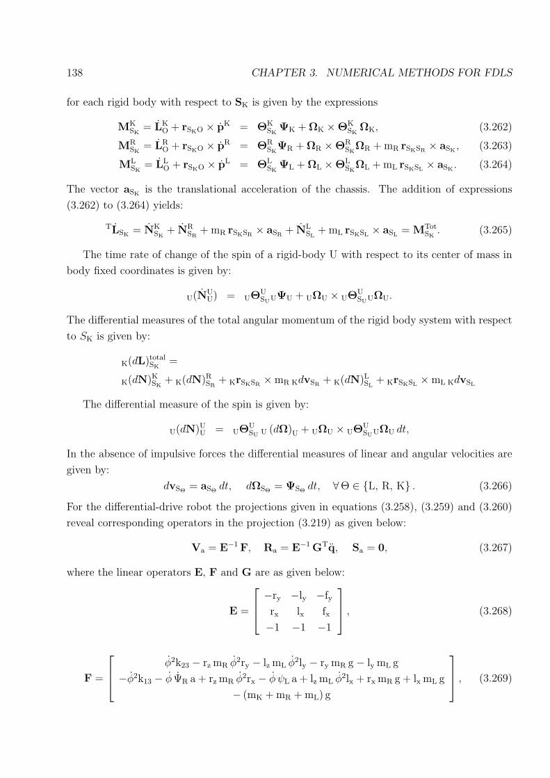
138 CHAPTER 3. NUMERICAL METHODS FOR FDLS
for each rigid body with respect to SK is given by the expressions
MKSK
= LKO + rSKO × pK = ΘK
SKΨK + ΩK ×ΘK
SKΩK, (3.262)
MRSK
= LRO + rSKO × pR = ΘR
SKΨR + ΩR ×ΘR
SKΩR + mR rSKSR
× aSK, (3.263)
MLSK
= LLO + rSKO × pL = ΘL
SKΨL + ΩL ×ΘL
SKΩL + mL rSKSL
× aSK. (3.264)
The vector aSKis the translational acceleration of the chassis. The addition of expressions
(3.262) to (3.264) yields:
TLSK= NK
SK+ NR
SR+ mR rSKSR
× aSR+ NL
SL+ mL rSKSL
× aSL= MTot
SK. (3.265)
The time rate of change of the spin of a rigid-body U with respect to its center of mass in
body fixed coordinates is given by:
U(NUU) = UΘU
SUUΨU + UΩU × UΘUSUUΩU.
The differential measures of the total angular momentum of the rigid body system with respect
to SK is given by:
K(dL)totalSK
=
K(dN)KSK
+ K(dN)RSR
+ KrSKSR×mR KdvSR
+ K(dN)LSL
+ KrSKSL×mL KdvSL
The differential measure of the spin is given by:
U(dN)UU = UΘU
SU U (dΩ)U + UΩU × UΘUSUUΩU dt,
In the absence of impulsive forces the differential measures of linear and angular velocities are
given by:
dvSΘ= aSΘ
dt, dΩSΘ= ΨSΘ
dt, ∀Θ ∈ L, R, K . (3.266)
For the differential-drive robot the projections given in equations (3.258), (3.259) and (3.260)
reveal corresponding operators in the projection (3.219) as given below:
Va = E−1 F, Ra = E−1 GTq, Sa = 0, (3.267)
where the linear operators E, F and G are as given below:
E =
−ry −ly −fy
rx lx fx
−1 −1 −1
, (3.268)
F =
φ2k23 − rz mR φ2ry − lz mL φ2ly − ry mR g − ly mL g
−φ2k13 − φ ΨR a + rz mR φ2rx − φ ψL a + lz mL φ2lx + rx mR g + lx mL g
− (mK + mR + mL) g
, (3.269)

3.8. NUMERICAL RESULTS 139
G =
− sin(φ)rz mR − sin(φ)lz mL − cos(φ)rz mR − cos(φ)lz mL 0
cos(φ)rz mR + cos(φ)lz mL − sin(φ)rz mR − sin(φ)lz mL 0
−k13 + rz mR rx + lz mL lx −k23 + rz mR ry + lz mL ly 0
−a 0 0
−a 0 0
. (3.270)
Further, if all three contacts belong to the index set IS, which is the case in the maneuvers of
the robot based on the assumptions, then:
Va = Vv, Rv = E−1 GTdu, Sv = 0 (3.271)
is valid.
3.8 Numerical Results
In this section four maneuvers are presented. The goal function f(y) in (3.244) becomes
f(y) = tf (3.272)
in the time-optimal case; or
f(y) =tf
Nc
Nc∑i=1
ML(i)2 + MR(i)2 (3.273)
in the control-effort case. The control moments of both wheels are limited to ‖ML‖ = 1 Nm and
‖MR‖ = 1 Nm, respectively. A number of 300 discretisation points are used and the controls
are discretized with 60 points each. The numerical values which are used in the optimisation
are given in table 4.3 and 5.1. In all maneuvers the robot starts at the origin given by:
[x0, y0, φ0, ψL0, ψR0
]=
[0, 0, 0, 0, 0
]
and [x0, y0, φ0, ψL0, ψR0
]=
[0, 0, 0, 0, 0
].
In all the maneuvers, the robot stops at final time:
[xf , yf , φf , ψLf , ψRf
]=
[0, 0, 0, 0, 0
].

140 CHAPTER 3. NUMERICAL METHODS FOR FDLS
ε 0.1 tfmin 2
c 103 tfmax 5
cd 106 Mmin −1
Toliter 10−7 Mmax 1
ct 106 Nc 60
Ns 300
Table 3.12: Numerical parameters of the optimisations in Maneuvers A, B, C and D. Here
ct and cd are penalties imposed on contraints on end time and on the deviation from the
final state, respectively.
3.8.1 Case A
The desired end position qd to be reached time-optimally is given by:
[xf , yf , φf , ψLf , ψRf
]=
[1, 5, −π
2, free, free
].
Maneuver A is characterized by a high dynamical activity in the orientation of the chassis.
The robot accomplishes this task in 4.03 seconds and the squared sum of the control effort is
3.73 N2 m2s. In order to orient itself to φ = −π2
time-optimally in the final part of the maneuver
the system performs a swing in maneuver during which it is in a five-DOF mode. At the
beginning the system rushes onto trajectory in the vicinity x = 1 and swings counterclockwise
out in order to have enough angular displacement to perform the swinging in the clockwise
direction as can be seen in figure 3.43. Figure 3.41 shows the contact forces during the maneuver
which are obtained by dividing the discretised differential measures of contact forces by the
discretisation interval. The same figure shows the absolute values of the relative tangential
contact velocities, which are used to analyse the mode behaviour of the system.
3.8.2 Case B
In maneuver B the task is to reach the following position qd control-effort optimally:
[xf , yf , φf , ψLf , ψRf
]=
[1, 5, −π
2, free, free
].
The robot accomplishes this task in 4.21 seconds and the squared sum of the control effort is
3.57 N2 m2s. As can be seen in figure 3.44 the CM of the robot traces a relatively straight line
until the final reorientation maneuver during which dissipates kinetic energy in the process of
brake down by the making use of the frictional work at the wheel contacts. The energy to the
system is delivered by the control effort and in the case where the control effort is minimised, it

3.8. NUMERICAL RESULTS 141
0 1 2 3 440
50
60
70
80
time in [sec]
[N]
Normal contact forces
λ NR
λ NL
λ NF
0 1 2 3 4
−40
−30
−20
−10
0
10
20
time in [sec]
[N]
Friction forces on the right wheel
λ TRx
λ TRy
0 1 2 3 4
−40
−20
0
20
time in [sec]
[N]
Friction forces on the left wheel
λ TLx
λ TLy
0 1 2 3 4
−2
0
2
4
6
time in [sec]
[m/s
]
Magnitudes of relative contact velocities
γR
γL
γF
Figure 3.41: Case A: Contact forces and contact relative velocities.
is intuitively clear that the system tends not to dissipate energy at wheel contacts unnecessarily.
As a consequence the Lagrangian system moves more in the non-dissipative two-DOF mode
in the first half of the maneuver where the system is accelerated. Dissipation is preferred in
order to brake down the system instead of making use of the control effort. In comparison
to the time-optimal maneuver A, it moves less in dissipative modes which can also be seen in
the trends of the magnitudes of the relative contact velocities of figures 3.41 and 3.42. The
evolution of the center of mass trajectories in the x-y plane for maneuvers A and B can be
seen in figures 3.47 and 3.48, respectively. The evolution of final time tf over the successive
minimisation of the augmented Lagrangian in both cases are depicted in figures 3.45 and 3.46,
respectively.
3.8.3 Case C
In maneuver C the task is to reach the following position qd time-optimally:
[xf , yf , φf , ψLf , ψRf
]=
[2, 5, 0, free, free
].
The robot accomplishes this task in 3.40 seconds and the squared sum of the control effort
is 5.35 N2 m2s. As can be seen in figures 3.49 and 3.51 the CM of the robot traces a straight

142 CHAPTER 3. NUMERICAL METHODS FOR FDLS
0 1 2 3 440
50
60
70
80
time in [sec]
[N]
Normal contact forces
λ NR
λ NL
λ NF
0 1 2 3 4
−40
−30
−20
−10
0
10
20
time in [sec]
[N]
Friction forces on the right wheel
λ TRx
λ TRy
0 1 2 3 4
−40
−20
0
20
time in [sec]
[N]
Friction forces on the left wheel
λ TLx
λ TLy
0 1 2 3 4
−2
0
2
4
6
8
time in [sec]
[m/s
]
Magnitudes of relative contact velocities
γR
γL
γF
Figure 3.42: Case B: Contact forces and contact relative velocities.
−3 −2 −1 0 1 2 3 4−1
0
1
2
3
4
5
6
CM position in [m]
CM
pos
ition
in [m
]
2−DOF mode
3−DOF mode
5−DOF mode
Figure 3.43: Case A: Number of DOF
during the maneuver.
−3 −2 −1 0 1 2 3 4−1
0
1
2
3
4
5
6
CM position in [m]
CM
pos
ition
in [m
]
2−DOF mode
3−DOF mode
5−DOF mode
Figure 3.44: Case B: Number of DOF
during the maneuver.

3.8. NUMERICAL RESULTS 143
5 10 15 202.8
3
3.2
3.4
3.6
3.8
4
Change of the endtime tf
Optimization number k
[sec
]
Figure 3.45: Case A: The final time tf
during successive minimisations.
2 4 6 8 10 12 14 16 18
3
3.5
4
Change of the endtime tf
Optimization number k
[sec
]
Figure 3.46: Case B: The final time tf
during successive minimisations.
0 1 2 3 4 5
−0.5
0
0.5
1
1.5
2
2.5
Final and intermediate trajectories of CM
y in [m]
x in
[m]
Figure 3.47: Case A: The evolution of
the trajectory of the CM.
0 1 2 3 4 5
−0.5
0
0.5
1
1.5
2
2.5
Final and intermediate trajectories of CM
y in [m]
x in
[m]
Figure 3.48: Case B: The evolution of
the trajectory of the CM.
−3 −2 −1 0 1 2 3 4 5−1
0
1
2
3
4
5
6
CM position in [m]
CM
pos
ition
in [m
]
2−DOF mode
3−DOF mode
5−DOF mode
Figure 3.49: Case C: Number of DOF
during the maneuver.
−3 −2 −1 0 1 2 3 4 5−1
0
1
2
3
4
5
6
CM position in [m]
CM
pos
ition
in [m
]
2−DOF mode
3−DOF mode
5−DOF mode
Figure 3.50: Case D: Number of DOF
during the maneuver.

144 CHAPTER 3. NUMERICAL METHODS FOR FDLS
Figure 3.51: Case C: Control Moments and phases of chassis DOF.
Figure 3.52: Case D: Control Moments and phases of chassis DOF.

3.8. NUMERICAL RESULTS 145
5 10 15 20 25 30 35 40
3
3.2
3.4
3.6
Change of the endtime tf
Optimization number k
[sec
]
Figure 3.53: Case C: Final time tf .
5 10 15 20 25 30 35 40
2.9
3
3.1
3.2
3.3
3.4
3.5
Change of the endtime tf
Optimization number k
[sec
]
Figure 3.54: Case D: Final time tf .
5 10 15 20 25 30 35 40
5
5.5
6
6.5
Change of Control Effort
Optimization number k
[N2 m
2 sec
]
Figure 3.55: Case C: The control effort.
5 10 15 20 25 30
4
5
6
7
Change of Control Effort
Optimization number k
[N2 m
2 sec
]
Figure 3.56: Case D: The control effort.
0 1 2 3
50
60
70
80
time in [sec]
[N]
Normal contact forces
λ NR
λ NL
λ NF
0 1 2 3
−40
−20
0
20
time in [sec]
[N]
Friction forces on the right wheel
λ TRx
λ TRy
0 1 2 3
−40
−20
0
20
time in [sec]
[N]
Friction forces on the left wheel
λ TLx
λ TLy
0 1 2 3
0
5
10
time in [sec]
[m/s
]
Magnitudes of relative contact velocities
γR
γL
γF
Figure 3.57: Case C: Contact forces and contact relative velocities.

146 CHAPTER 3. NUMERICAL METHODS FOR FDLS
0 1 2 3
50
55
60
65
70
75
time in [sec]
[N]
Normal contact forces
λ NR
λ NL
λ NF
0 1 2 3
−40
−20
0
20
time in [sec]
[N]
Friction forces on the right wheel
λ TRx
λ TRy
0 1 2 3
−40
−20
0
20
time in [sec]
[N]
Friction forces on the left wheel
λ TLx
λ TLy
0 1 2 3
−1
0
1
2
3
4
5
time in [sec]
[m/s
]
Magnitudes of relative contact velocities
γR
γL
γF
Figure 3.58: Case D: Contact forces and contact relative velocities.
Figure 3.59: Case C: Contact forces and contact relative velocities.

3.8. NUMERICAL RESULTS 147
Figure 3.60: Case A: Control Moments and phases of chassis DOF.
Figure 3.61: Case B: Control Moments and phases of chassis DOF.

148 CHAPTER 3. NUMERICAL METHODS FOR FDLS
line as would be expected from a time-optimal solution. Since a straight line is the shortest
distance that connects two points, a straight line trajectory between end point and final point
is obtained as a result of the optimisation. One can recognise three phases of the maneuver. In
the first phase of the motion the chassis is oriented approximately to the angle 21.8o which is
the angle between initial and final point. In the second phase the robot accelerates on the line
as can be seen in figure 3.51. In the third phase of the motion the robot reorients itself to the
orientation φ = 0. In the second phase of the motion due to asymmetrical loading conditions
on the left and right wheels as can be inferred from the normal force trends in figure 3.57,
the orientation tends to deviate from the set course. Since the chassis degrees of freedom are
steered through the set-valued coupling to the control forces, the system undergoes successive
stick-slip transitions on the right wheel in order to maintain orientation, which is depicted in
figure 3.57 in the trends of |γR|, |γL| and |γF|. It is obvious that given enough time that the
system would find a solution that always moves in the 2-DOF mode, but as the final time is
reduced and the control forces are driven to the allowable limits it is not possible for the system
to stay always in sticking with both wheels.
3.8.4 Case D
In maneuver D the task is to reach the following position qd control-effort optimally:
[xf , yf , φf , ψLf , ψRf
]=
[2, 5, 0, free, free
].
As can be seen in figures 3.50 and 3.52 the CM of the robot traces a relatively straight line
and the dissipative modes are avoided during acceleration and occur only during deceleration.
The robot accomplishes this task in 3.47 seconds and the squared sum of the control effort is
5.02 N2 m2s. A similar three phase structure for the maneuver D is recognisable as in maneuver
C but the robot spends less effort to trace a straight line, which would require intensive course
correction actions. In order to save up control effort, the system makes use of frictional dissi-
pation in order to brake down the system velocity and moves longer in the 5-DOF mode in the
deceleration of the system. In comparison to the time-optimal maneuver C, it moves during
the braking phase in dissipative modes which can also be seen in the trends of the magnitudes
of the relative contact velocities of figures 3.57 and 3.58. The evolution of final time tf over the
successive minimisation of the augmented Lagrangian in both cases are depicted in figures 3.53
and 3.54, respectively. The evolution of total control effort over the successive minimisation of
the augmented Lagrangian in both cases are depicted in figures 3.55 and 3.56, respectively.

3.8. NUMERICAL RESULTS 149
0 50 100 150 200 250 300−0.3
−0.2
−0.1
0
0.1
interval number on the partition
[J]
Numerical Error in the Energy Balance
2−DOF mode
3−DOF mode
5−DOF mode
Figure 3.62: ∆T jerr for Maneuver A.
0 50 100 150 200 250 300
−0.2
−0.1
0
0.1
interval number on the partition
[J]
Numerical Error in the Energy Balance
2−DOF mode
3−DOF mode
5−DOF mode
Figure 3.63: ∆T jerr for Maneuver B.
0 50 100 150 200 250 300−0.3
−0.25
−0.2
−0.15
−0.1
−0.05
0
interval number on the partition
[J]
Numerical Error in the Energy Balance
2−DOF mode
3−DOF mode
5−DOF mode
Figure 3.64: ∆T jerr for Maneuver C.
0 50 100 150 200 250 300
−0.06
−0.04
−0.02
0
0.02
interval number on the partition
[J]
Numerical Error in the Energy Balance
2−DOF mode
3−DOF mode
5−DOF mode
Figure 3.65: ∆T jerr for Maneuver D.
10 15 20 25 30 35 40 4590
91
92
93
94
95
96
97
Optimization number k
%
Ratio of Control Work to Total Dissipation
ABCD
Figure 3.66: WC
WDfor Maneuvers in
intermediate Optimisation stages.
10 15 20 25 30 35 40 45−8
−6
−4
−2
0
2
4
6
Optimization number k
[J]
WC+W
D
ABCD
Figure 3.67: WC + WD for Maneuvers in
intermediate Optimisation stages.

150 CHAPTER 3. NUMERICAL METHODS FOR FDLS
0 50 100 150 200 250 300−100
0
100
200
300
Partition Interval
[J]
Figure 3.68: Case A: Errors in Energy.
0 50 100 150 200 250 300−50
0
50
100
150
200
Partition Interval
[J]
Figure 3.69: Case B: Errors in Energy.
0 50 100 150 200 250 300−30
−20
−10
0
10
20
Partition Interval
[J]
∆ Terr
−∆ Terr,1
−∆ Terr,2
(10−4)
∆ Terr,1
(10−2)
∆ Terr,2
(10−4)
Figure 3.70: Case C: Errors in Energy.
0 50 100 150 200 250 300
0
20
40
60
80
Partition Interval
[J]
Figure 3.71: Case D: Errors in Energy.
3.8.5 Simplectic and Dissipative Properties of the Sweeping Process
The advantages of Moreau’s discretisation scheme have a price because it introduces a certain
error in the energy balance. The Lagrangian of the switching Lagrangian system is defined as:
L(q,u) = T (q,u)− V (q). (3.274)
Here T (q,u) denotes the total kinetic, and V (q) the total smooth potential energy of the
system. The total energy of the system is:
H(q,u) = T (q,u) + V (q). (3.275)
The differential measure of the energy H is given by:
dH(q,u) =dH
dtdt +
(T+ − T−)
dσ. (3.276)
If the Lebesgue-Stieltjes Integral of the differential measure of the kinetic energy over an atomic
time instant is evaluated then one obtains:∫
tidT = T+ − T−. (3.277)

3.8. NUMERICAL RESULTS 151
The Borel measurable part of H is related to the jump in kinetic energy:
T+ − T− =1
2
⟨u+, M(q)u+
⟩− 1
2
⟨u−, M(q)u−
⟩, (3.278)
and is nonzero if and only if there is an impulsive action that induces a jump in the generalised
velocities. For the class of switching Lagrangian systems defined by relations (3.224) to (3.226)
the differential measure of total energy is equal to the sum of the differential measure of the
work of control forces dWC and the differential measure of the dissipative work dWD as stated
below:
dH = dWC + dWD. (3.279)
Here dWC and dWD are defined by:
dWC =⟨u−, B(q) τ−
⟩dt (3.280)
and
dWD =∑
∀ i∈IS
⟨1
2
(γ−Ti
+ γ+Ti
), dΛTi
⟩, (3.281)
respectively. The difference between the kinetic energies at successive discretisation points is
given by:
∆ T j = T j+1 − T j =⟨uj+1, M(qj+1)uj+1
⟩− ⟨uj, M(qj)uj
⟩(3.282)
≈ 1
2
⟨uj+1, M(qj
m)uj+1⟩− 1
2
⟨uj, M(qj
m)uj⟩
(3.283)
=1
2
⟨uj+1 − uj, M(qj
m)(uj+1 + uj
)⟩(3.284)
and the difference in potential energy is approximated by:
∆ V j = V j+1 − V j ≈ ⟨uj+1,hpot(q
j+1)⟩ ∆ t
2+
⟨uj,hpot(q
j)⟩ ∆ t
2(3.285)
=⟨uj + uj+1,hpot(qm)
⟩ ∆ t
2=
⟨qj+1 − qj,hpot(qm)
⟩. (3.286)
Here the vector h(q,u) is separated in its potential and nonpotential parts:
h(q,u) = hnonpot(q,u) + hpot(q). (3.287)
The discretized approximations of the differential measures of control work and dissipative
work are given by:
∆W jC =
⟨uj, B(qj
m) τ j⟩
∆t, (3.288)
∆W jD =
∑
∀ i∈IS
⟨1
2
(γj
Ti+ γj+1
Ti
), Λj
Ti
⟩. (3.289)

152 CHAPTER 3. NUMERICAL METHODS FOR FDLS
The evaluation of the dissipation unifies in it the impulse and the force character. Though ΛTi
is an impulse and is seen mathematically as a distribution on its support, by assuming that it
has a constant density on its support, which in this case has the measure ∆ t, is equivalently
represented as ΛTi= λTi
∆ t. Here λTiis a force and the value of the constant density on
the support. By making use of this distributional approach, the work of the frictional contact
impulses can be evaluated like forces. The question that poses itself is now naturally to define
the instant at which this force acts in order to obtain its work contribution by dual pairing
with a suitable velocity. Here one notices that this force equally distributed over the support
and the midpoint velocity on the support as used in ∆W jD turns out to be suitable. The energy
balance over an interval then reads:
∆ V j + ∆ T j −∆W jC −∆W j
D = ∆ H jerr. (3.290)
Insertion of the discretized form of the measure-differential inclusion as given below in the
expression for ∆ T j :
uj+1 − uj = M−1(qjm)
(h(qj
m, uj) ∆ t +∑
∀ i∈IS
WTi(qm)ΛTi
+ B(qm)τ j∆ t
), (3.291)
and considering γjTi
+γj+1Ti
= WTTi
(qm)(uj
Ti+ uj+1
Ti
)reveals the expression for the error ∆ H j
err
for interval j as:
∆ H jerr ≈ ∆ t
2
(⟨uj+1 − uj, B(qj
m) τ j⟩
+⟨uj+1 + uj, hnonpot(q
jm, uj)
⟩)(3.292)
= ∆ H jerr,1 + ∆ H j
err,2.
The expressions ∆ H jerr,1 and ∆ H j
err,2 are defined as:
∆ H jerr,1 =
∆ t
2
⟨uj+1 − uj, B(qj
m) τ j⟩
(3.293)
and
∆ H jerr,2 =
∆ t
2
⟨uj+1 + uj, hnonpot(q
jm, uj)
⟩, (3.294)
respectively. The analysis of the energy balance for the differential-drive robot provides a
visualisation of the inherent energy deficiency. For a mechanical system like the differential-
drive robot where there are no changes in the gravitational potential and V (q) is constant
throughout, one has: ∫ tf
t0
dT =
∫ tf
t0
dWC + dWD = 0, (3.295)
if the generalised velocities are zero at t0 and tf . In this case the error in the energy balance
∆ H jerr is set equal to ∆ T j
err.

3.8. NUMERICAL RESULTS 153
Figure 3.72: Case B: Evolution and Convergence Behaviour of x and x trajectories.
Figure 3.66 indicates the ratio WC
WDfor the maneuvers A, B, C, D in the intermediate changes
of the optimisation, whereas figure 3.67 depicts the energy deficiency in Joules for the same
cases. Figures 3.62 to 3.65 show for the cases A, B, C and D the numerical values of ∆ H jerr and
the color code indicates in which mode the robot moves for given energy deficiency. Figures 3.68
to 3.71 reflect the magnitude plots of ∆ T jerr,1 and ∆ T j
err,2 as calculated by equations (3.293)
and (3.294), and ∆ T jerr − ∆ T j
err,1 − ∆ T jerr,2 where ∆ T j
err is obtained by (3.290) by setting
∆ T jerr = ∆ H j
err .
3.8.6 Convergence Behaviour of Case B
In this subsection the evolution of various trajectories for Case B is presented. The optimal re-
sult in Case B is obtained after 15 successive minimisation stages. Quantitatively the evolution
of the phase trajectories in Maneuver B as visualized in figure 3.77 is an indication of the global
optimizing behaviour of the proposed algorithm. Figures 3.72, 3.73, 3.74, 3.75 and 3.76 show
the evolution of respective trajectories and the logarithm of the distance of successive trajec-
tories together. It is characteristic that at the solution as a result of the convergent behaviour
of the algorithm the distance between successive trajectories gets very small. This convergent
behaviour is seen in the evolution of the generalised positions and velocities in figures 3.72,
3.73, 3.74, 3.75 and 3.76.
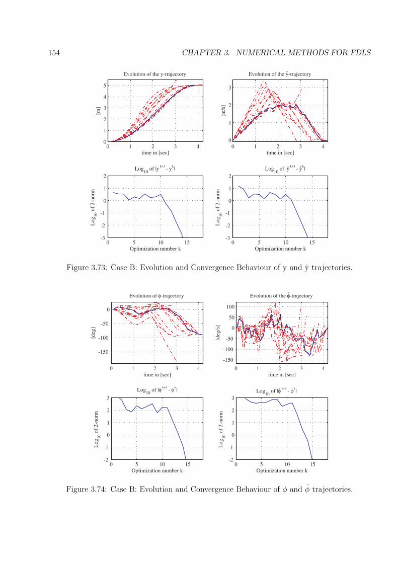
154 CHAPTER 3. NUMERICAL METHODS FOR FDLS
Figure 3.73: Case B: Evolution and Convergence Behaviour of y and y trajectories.
Figure 3.74: Case B: Evolution and Convergence Behaviour of φ and φ trajectories.

3.8. NUMERICAL RESULTS 155
Figure 3.75: Case B: Evolution of ΨR, ΨL, ΨR and ΨL trajectories.
0 1 2 3 4−2
−1
0
1
2Evolution of left−wheel moment
time in [sec]
[Nm
]
0 5 10 15−3
−2
−1
0
1
Log10
of |MLk+1−M
Lk |
Optimization number k
Log 10
of 2
−no
rm
0 1 2 3 4−2
−1
0
1
2Evolution of right−wheel moment
time in [sec]
[Nm
]
0 5 10 15−3
−2
−1
0
1
Log10
of |MRk+1−M
Rk |
Optimization number k
Log 10
of 2
−no
rm
Figure 3.76: Case B: Evolution and Convergence Behaviour of ML and MR trajectories.

156 CHAPTER 3. NUMERICAL METHODS FOR FDLS
Figure 3.77: Case B: Evolutions of DOF x,y and φ as phase diagrams.

Chapter 4
Internal Boundary Variations,
Discontinuous Transversality
Conditions and Optimal Control
In this work, necessary conditions for the impulsive optimal control of multibody mechanical
systems are stated. The conditions are obtained by the application subdifferential calculus tech-
niques to extended-valued lower semi-continuous generalised Bolza functional that is evaluated
on multiple intervals. Contrary to the approach in literature so far, an instant at which possibly
impulsive transition takes place is considered as a Lebesgue negligible instant. This approach
is in comparison to other impulsive necessary conditions consistent with mainstream hybrid
system modeling methods in which transitions happen instantaneously. The necessary condi-
tions provide necessary criteria for the determination of optimal transition times and locations.
The consideration of certain type of variations at the boundaries give birth to the concepts
of internal boundary variations and discontinuous transversality conditions. The concepts are
developed by the author and are presented and discussed in [110] and [112] with applications
to optimal control. In this work, a characterisation of these concepts in terms of upper and
lower subderivatives to the extended-valued lower-semicontinuous value functional under several
regularity assumptions is given. The properties of the transition sets are discussed.
4.1 Introduction
An impact in mechanics is defined as a discontinuity in the generalised velocities of a mechan-
ical system which is induced by impulsive forces, therefore optimal control of such impulsive
systems inevitably encompasses optimal control with discontinuous generalised velocities. The
main issue in the optimal control of impactive mechanical systems has been the blending of
impact mechanics with impulsive optimal control. The crux in the derivation of these necessary
157
158 CHAPTER 4. DISCONTINUOUS TRANSVERSALITY AND IMPULSIVE CONTROL
conditions is to handle joint discontinuity of the state and the dual state on a Lebesgue negligi-
ble interval. In the framework of integration theory, this has long been recognised as a problem
if state and costate should become concurrently discontinuous as has been addressed in [64]
by Moreau and [82] by Rockafellar. Rockafellar studied in [82] the discontinuity of the dual
state in constrained convex optimal control problems but dispensed of attacking the problem
concurrent discontinuity of state and costate. Moreau gave in [64] partial integration formulas
for differential measures in general bilinear forms. In [68] Murray studies the extension and
existence theorems of problems in calculus of variation to the setting when impulsive controls
are applied and state discontinuity occurs. He bases his work on [82], and outlines in his mo-
tivation that jumps in the states may occur due to constraints on the dual dynamics which
are reached by the costate and considers applications in the field of economics. In [18] several
classes of impulsive Lagrangian systems are studied by Bressan. The main focus is impulses
generated by sudden parameter changes such as inertial parameters that affect the momentum
balance, or impulses arising due to structure of constraints of a mechanical system. A certain
class of impulsive systems that resemble discontinuous diffusion processes are treated in [12] by
Bensoussan.
In what follows next, the new concepts required to deal with this specific problem are intro-
duced. In order to overcome the difficulties arising from joint discontinuity of state and costate,
the instant of impulsive control action where discontinuity in the generalised velocities occur is
considered as an internal boundary in the time domain. In [112] by Yunt, the concept of internal
boundary variations are introduced literally, and as an application a theorem that states the
necessary conditions for the impulsive time-optimal control of finite-dimensional Lagrangian
systems is stated. In the framework of these concepts, philosophically, the instant of state dis-
continuity constitutes an internal boundary in the optimal control problem. The essential idea
is thus to consider every point of the domain where continuity and differentiability ceases to
exist, as a boundary of the problem. By introducing a boundary at an instant of a discontinuity,
one has to notice that it has bilateral character, in the sense that the boundary constitutes an
upper boundary for one segment of the interval whereas for the other segment a lower bound-
ary in the time domain. The necessity that at a location of transition several conditions have
to be fulfilled, gives rise to the idea of some sort of transversality conditions if one begins to
consider an instant of discontinuity as a two-sided boundary where to arcs are ”connected”
discontinuously. This dependence is embedded in the concept of internal boundary variations.
In order to obtain criteria for the optimality of the transition position, transition pre-, and
post-transition generalised velocities, transition time and impulsive control, variations in these
entities need to be considered, which represent in the setting of this work the internal boundary
variations. At the boundaries of the time domain, the pre-transition state variations are consid-
ered separately from the post-transition variations. The absolute continuity of the generalised

4.2. PRELIMINARIES 159
positions means that the total variation of the generalised positions at the pre-transition and
post-transition instants are equal. The pre-transition and post-transition variations are inter-
related by the transition conditions which can be seen as the bases of transversality conditions
that join two trajectories discontinuously. The transition conditions are introduced symmet-
rically with respect to pre-, and post-transition states. The transition conditions are of two
types, namely, the impact equation and the constitutive impact laws. The impact equations re-
late the discontinuity in the impulse of the Lagrangian system to the impulsive forces/controls.
The impact law (.i.e. the moreau-newton impact law), however, is a constitutive law which is
chosen depending on the modeling approach preferred. As a case study, in reference [111] the
blocking of some DOF of an underactuated manipulator by tangential fully-inelastic impact is
discussed and the necessary conditions are stated. In [110] the necessary conditions for the im-
pulsive optimal control of Lagrangian systems in the Hamiltonian framework is investigated. By
the application of subdifferential calculus techniques to extended-valued lower semi-continuous
functionals, necessary conditions are obtained. In publications of R. T. Rockafellar such [84]
and [85] a summary of the rules in subdifferential calculus are provided, which is one of the
most flourishing branches of mathematics.
4.2 Preliminaries
Definition 4.1.1 The Proximal Normal Vector Given a closed set C ∈ Rk and a point
x ∈ C, a vector et ∈ Rk is called to be a proximal normal vector to C at x if there exists M ≥ 0
such that
〈η,x− x〉 ≤ M |x− x|2 ,∀x ∈ C. (4.1)
Definition 4.1.2 The Proximal Normal Cone The cone of all proximal normal vectors η
to C is called the proximal normal cone to C at x and is denoted by N PC (x):
N PC (x) :=
η | 〈η,x− x〉 ≤ M |x− x|2 ,∀x ∈ C, et ∈ Rk : ∃M ≥ 0
. (4.2)
Definition 4.1.3 The Limiting Normal Vector Given a closed set C ∈ Rk and a point
x ∈ C, a vector et ∈ Rk is called to be a limiting normal vector to C at x ∈ C if there exist
sequences xi−→C x and ηi → η such that
ηi ∈ N PC (xi), ∀i. (4.3)
Definition 4.1.4 The Limiting Normal Cone The cone of limiting normal vectors to Cat x is denoted NC(x) and is defined by:
NC(x) :=et ∈ Rk |∃xi
−→C x ∧ ηi → η,ηi ∈ N PC (xi), ∀i
. (4.4)

160 CHAPTER 4. DISCONTINUOUS TRANSVERSALITY AND IMPULSIVE CONTROL
Definition 4.1.5 The Strict Normal Vector and Strict Normals Given a closed set
C ⊂ Rk and a point x ∈ C, the strict normal cone to C at x, written NC(x), is the set
NC(x) :=
p | lim sup
y−→C x
〈p, y − x〉|y − x| ≤ 0
. (4.5)
Elements in NC(x) are called strict normals to C at x.
Some elementary properties of the cones that have been introduced are listed without proof.
Proposition 4.1.1 Take a closed set C ⊂ Rk and points x ∈ C and p ∈ Rk. Then the following
assertions are equivalent:
1. p ∈ NC(x),
2. there exist sequences and such that pi ∈ NC(x), ∀i.
Proposition 4.1.2 Take a closed set C ⊂ Rk and points x ∈ C. Then:
1. NC(x), N PC (x) and NC(x) are all cones in Rk, containing 0 and
N PC (x) ⊂ NC(x) ⊂ NC(x); (4.6)
2. N PC (x) is convex, but not necessarily closed;
3. NC(x) is closed and convex;
4. the set-valued mapping y → NC(y) : C → Rk has a closed graph, in the sense that, for
any sequences yi−→C y and pi → p such that pi ∈ NC(yi) for all i, we have p ∈ NC(x).
Proposition 4.1.3 Take a closed set C ⊂ Rk and a point x ∈ C. Then:
1. x ∈ intC implies NC(x) = 0.
2. x ∈ bdyC implies NC(x) contains nonzero elements.
Proposition 4.1.4 Take closed subsets C1 ⊂ Rm and C2 ⊂ Rn , and a point (x1,x2) ∈ C1×C2.
Then
N PC1×C2(x1,x2) = N P
C1(x1)×N PC2(x2), (4.7)
NC1×C2(x1,x2) = NC1(x1)× NC2(x2), (4.8)
NC1×C2(x1,x2) = NC1(x1)×NC2(x2). (4.9)
Proposition 4.1.5 Take a closed convex set C ⊂ Rk and a point x ∈ C. Then
NC(x) = N PC (x) = NC(x) = ξ | ξ, 〈x− x〉 ≤ 0, ∀x ∈ C. (4.10)

4.2. PRELIMINARIES 161
Definition 4.1.6 The Proximal Subgradient Given an extended-valued, lower semi-
continuous function f : Rk → R ∪∞ and a point x ∈ dom f. A vector et ∈ Rk is said to be
a proximal subgradient of f at x if there exist ε > 0 and M ≥ 0 such that
〈η,x− x〉 ≤ M |x− x|2 ,∀x that satisfy |x− x| ≤ ε. (4.11)
Definition 4.1.7 The Proximal Subdifferential The set of all proximal subgradients of
f at x is called the proximal subdifferential of f at x and is denoted by ∂P f(x).
Definition 4.1.8 The Limiting Subdifferential Given f : Rk → R ∪ ∞ and a point
x ∈ dom f. A vector et ∈ Rk is said to be a limiting subgradient of f at x if there exist
sequences such that xi−→f x and ηi → η such that
ηi ∈ ∂P f(xi), ∀i. (4.12)
The upper subderivative and the lower subderivative of an extended-valued lower semicon-
tinuous (l.s.c) function is defined as given [85].
Definition 4.1.8 Upper and Lower Subderivatives [85] Let f be any extended-real
valued lower semi-continuous function on a linear topological space E , and let x be any point
where f is finite. The upper subderivative of f at x with respect to y is defined by:
f ↑(x;y) = lim sup
x′−→f x
t ↓ 0
infy′→y
f(x′ + ty′)− f(x′)t
. (4.13)
The lower subderivative of f at x with respect to y is defined by:
f ↓(x;y) = lim infx′−→f x
t ↓ 0
supy′→y
f(x′ + ty′)− f(x′)t
, (4.14)
where
x′−→f x ⇔ x′ ⇒ x ∧ f(x′) ⇒ f(x).
Theorem 4.1.1 (Theorem (4) in [85]) Let f be any extended-real valued function on a linear
topological space E , and let x be any point where f is finite. Then the ”upper” subdifferential
∂f(x) is a weak∗-closed convex subset of E∗ and
∂f(x) =
z ∈ E∗ | (z,−1) ∈ Nepi f (x, f(x))
. (4.15)
If f ↑(x ; 0) = −∞, then ∂f(x) is empty, but otherwise ∂f(x) is nonempty and
f ↑(x ; y) = sup 〈y, z〉 | z ∈ ∂f(x), ∀y ∈ E . (4.16)

162 CHAPTER 4. DISCONTINUOUS TRANSVERSALITY AND IMPULSIVE CONTROL
Analogously, the ”lower” subdifferential ∂f(x) is a weak∗-closed convex subset of E∗ and
∂f(x) =
z ∈ E∗ | (z,−1) ∈ Nhypo f(x, f(x))
. (4.17)
If f ↓(x ; 0) = ∞, then ∂f(x) is empty, but otherwise ∂f(x) is nonempty and
f ↓(x ; y) = inf〈y, z〉 | z ∈ ∂f(x), ∀y ∈ E
. (4.18)
4.2.1 Regularity of Sets
In order to establish the relationship between the geometric concepts defined above and the
previously known ones in smooth contexts, a notion of regularity for sets is introduced. The
contingent cone KC(x) is the set of tangents to a set C at a point x. A vector v in X belongs
to KC(x) iff, for all ε > 0, there exists t in (0, ε) and a point w in v+ εB such that x+tw ∈ C.
TC(x) is always contained in KC(x), which is not always convex.
Definition 4.1.9 The set C is regular at x provided TC(x) = KC(x). This property implies
that KC(x) is convex if the set C is tangentially regular.
Definition 4.1.10 Subdifferential Regularity function f is called subdifferentially reg-
ular x if f is finite at x and
lim infy′ → y
t ↓ 0
f(x + ty)− f(x)
t= f ↑(x;y), ∀y. (4.19)
Theorem 4.1.2 (Rockafellar ) Each of the following implies that f is directionally Lips-
chitzian at x (a point where f is finite):
1. f is Lipschitzian on a neighborhood of x;
2. f is convex and bounded above on a neighborhood of some point (not necessarily x itself);
3. f is concave and bounded below on a neighborhood of some point (not necessarily x
itself);
4. f is non-decreasing with respect to the partial ordering of E induced by some closed
convex cone K with non-empty interior;
5. f is the indicator of a set C that is epi-Lipschitzian at x;
6. E = Rn, f is lower semicontinuous on a neighbourhood of x, and the cone y | f ↑(x;y)is not included in any subspace of lower dimension;

4.2. PRELIMINARIES 163
7. E = Rn, f is lower semicontinuous on a neighbourhood of x, and ∂ f(x) is non-empty and
does not include an entire line.
Proposition 4.1.6 Suppose C is a smooth manifold around x in the sense that
C = x | gj(x) = 0, for j = 1, . . . , r, (4.20)
where the functions gj are continuously differentiable around y and the gradients ∇gj(x), j =
1, . . . , r are linearly independent. Then KC(x) is convex, and in fact
KC(x) = y | 〈y, ∇gj(x)〉 = 0, for j = 1, . . . , r. (4.21)
Theorem 4.1.3 Let f1 and f2 be extended-real-valued functions on E that are finite at x.
Suppose that f2 is directionally Lipschitzian at x and
y | f ↑1 (x;y) < ∞⋂
inty | f ↑2 (x;y) < ∞ 6= ∅ (4.22)
Then
(f1 + f2)↑ (x;y) ≤ f ↑1 (x;y) + f ↑2 (x;y), ∀y (4.23)
∂ (f1 + f2) (x) ⊂ ∂f1(x) + ∂f2(x) (4.24)
Equality holds in 4.24 if f1 and f2 are also subdifferentially regular. It also holds in 4.23 if in
addition f ↑1 (x;y) and f ↑2 (x;y) are not −∞ (i.e. ∂f1(x) and ∂f2(x)) are nonempty ), and in
that event f1 + f2 is likewise subdifferentially regular.
Corollary 4.1.1 Suppose f1 is convex and finite at x and f2 is Lipschitzian on a neigh-
bourhood of x. Then
∂(f1 + f2)(x) ⊂ ∂f1(x) + ∂f2(x), (4.25)
and there is equality if f1 and f2 are also subdifferentially regular at x.
Corollary 4.1.2 Let C1 and C2 be subsets of E , and let x ∈ C1
⋂ C2. Suppose that
TC1(x)⋂TC2(x) 6= ∅, (4.26)
and that C2 is epi-Lipschitzian at x. Then
TC1∩C2(x) ⊃ TC1(x)⋂TC2(x) (4.27)
NC1∩C2(x) ⊂ NC1(x) +NC2(x) (4.28)
where the set on the right in (4.28) is weak∗-closed. Equality holds in (4.27) if C1 and C2 are
tangentially regular at x, and then C1
⋂ C2 is likewise tangentially regular.

164 CHAPTER 4. DISCONTINUOUS TRANSVERSALITY AND IMPULSIVE CONTROL
4.3 The Generalised Problem of Bolza in Impulsive Con-
trol Form for Rigidbody Lagrangian Systems
Consider a problem in Bolza form (GPB), in which the objective is to choose absolutely con-
tinuous arcs q ∈ AC and u ∈ AC in order to minimise problem P given by:
P : J(q,u) = l(q(a),u(a),q(b),u(b)) +
∫ b
a
L(t,q(t),u(t), u(t)) dt , (4.29)
where the function L : [a, b] × Rn × Rn × Rn → R ∪ +∞ is L × B measurable. Here L × Bdenotes the σ-algebra of subsets of [a, b]× Rn generated by product sets M×N , where M is
a Lebesgue measurable subset of [a, b] and N is a Borel subset of R3 n. For each t ∈ [a, b], the
function l and L are lower semi-continuous on Rn×Rn×Rn×Rn and Rn×Rn×Rn, respectively,
with values in R∪+∞. For each (t,q,u) in [a, b]×Rn×Rn, the function L(t,q,u, ·) is convex
and l represents the endpoint cost. GPB concerns the minimisation of a functional whose form
is identical to that in the classical calculus of variations. The endpoint cost l and the integrand
L are allowed to take the value +∞, so that a variety of endpoint and differential constraints
can be treated. An important class of optimal control problems constrain the derivative of an
admissible arc and can be formulated in the form:
minl(q(a),u(a),q(b),u(b)) : M(q) u(t) ∈ F(t,q,u) a.e. t ∈ [a, b]. (4.30)
The problem in (4.30) can be seen as minimising the Bolza functional J over all arcs q,u. If
one identifies the integrand in (4.29) with (4.31):
L(t,q,u, a) = ΨF(t,q,u)(a) =
0, ifM(q) a ∈ F(t,q,u) ,
else +∞ ,(4.31)
the general class of optimal control problems defined in (4.30) can be handled as a GPB. It is
evident that for some pair of arcs (q, u) one then has
∫ b
a
L(t,q,u, u) dt =
0, M(q) u(t) ∈ F(t,q,u) a.e. t ∈ [a, b],
+∞ .(4.32)
where the differential inclusion F is defined via the state-control triplet (τ ,q,u):
M(q) u(t) ∈ F(q,u) (4.33)
:= a |M(q) a = h(q(t),u(t)) + B(q(t)) τ (t) ∀τ (t) ∈ Cτ , a.e. t ∈ [a, b].
In order to guarantee the well-behaving of F and l let following assumptions hold:
Assumptions 4.1. A pair of trajectories of generalised positions q : [a, b] → Rn and
velocities u : [a, b] → Rn is given. On some relatively open subset Ω ⊆ [a, b] × Rn × Rn × Rn
containing the graph of (q, u), the following statements hold:

4.3. IMPULSIVE GENERALISED PROBLEM OF BOLZA 165
1. The multifunction F is L×B measurable on Ω. For each (t,q,u) in Ω, the set F(t,q,u)
is nonempty, compact and convex.
2. There are nonnegative integrable functions kq(t), ku(t) and Φ(t) on [a, b] such that
(a) F(t,q,u) ⊆ Φ(t)B for all q,u ∈ ΩT, almost everywhere, and
(b) F(t,q,u) ⊆ F(t,q,u) + kq(t)|p − r| + ku(t)|p − r|clB for all (p, p), (r, r) ∈ ΩT,
almost everywhere.
3. The endpoint cost function l is lower-semicontinuous on Ωa × Ωb.
Here ΩT is given by ΩT = (q,u) ∈ Rn × Rn | (t,q,u) ∈ Ω, ∀t ∈ [a, b]\ti ∈ IT and Bis the unit open ball. It is assumed that conditions of assumptions 4.1 are fulfilled for the
Lebesgue-measurable part of the Lagrangian dynamics in the ”almost everywhere” sense. By
the way ΩT is defined, the instants of the discontinuity are excluded.
Having set the stage, the necessary conditions for the impulsive optimal control problem of
finite-dimensional Lagrangian systems is formally derived by considering a problem in GPB, in
which the objective is to choose arcs q ∈ AC and u ∈ LBV on every interval(t+i , t−i+1
) ∈ IT
and transition location tripletsq(ti+1),u(t−i+1),u(t+
i ), transition times ti and final time tf ,
∀ ti ∈ IT in order to minimise PTot:
J(q(t),u(t),q(ti),u(t−i ),u(t+
i ), t−i , t+i
, tf) = (4.34)
N∑i=1
l(q(t−i+1),u(t−i+1),q(t+i ),u(t+
i )) +
∫ t−i+1
t+i
Li(si,q(si),u(si), u(si)) dsi .
The theory at hand treats optimal solutions as solutions of multi-point boundary value prob-
lems (MBVP) with discontinuous transitions in the state. In this setting, the prespecification of
the mode sequence and number of intervals must be given in advance. The overall problem as
stated in (4.34) is seen as the union of several problems in the generalised Bolza form. Here it
is assumed that the control horizon is composed of n different phases, which are separated from
eachother by N− 1 possibly discontinuous transitions in the generalised velocities. The impor-
tance of the transition process becomes clear if one considers the fact that at pre-transition and
post-transition states the values of several functions may differ due to discontinuities. A tran-
sition process is common to the pre-transition configuration and post-transition configuration.
Each problem Pi with a unique mechanical configuration is defined on a closed time domain
dom(Pi) with variable boundary which is partitioned as follows:
dom(Pi) =t−i , t+
i
⋃ (t+i , t−i+1
) ⋃ t−i+1, t+
i+1
. (4.35)
The boundary of the domain dom(Pi) is given by:
bdy dom(Pi) =t−i , t+
i
⋃ t−i+1, t+
i+1
. (4.36)

166 CHAPTER 4. DISCONTINUOUS TRANSVERSALITY AND IMPULSIVE CONTROL
The interior of the domain is given by:
int dom(Pi) =(t+i , t−i+1
). (4.37)
The domain of the overall problem PTot is given by the union:
dom(PTot) =⋃
∀ i
dom(Pi). (4.38)
However, the domains of successive problems Pi and Pi+1 are not disjoint:
dom(Pi)⋂
dom(Pi+1) = bdy dom(Pi)⋂
bdy dom(Pi+1) =t−i+1, t+
i+1
, (4.39)
The set bdy dom(Pi)⋂
bdy dom(Pi+1) =t−i+1, t+
i+1
is the support of the transition process
and is Lebesgue-negligible. The extended-valued integrand may differ on each interval based on
the structure of the equations of motion. The difference in structure may arise due to change in
parameters ( i.e. mass, inertia) or degrees of freedom. In [112] by Yunt a projection approach
is presented in case, the mechanical configurations in successive intervals differ based on change
in the number of degrees of freedom.
4.4 Statement of the Optimal Control Problem
The impulsive optimal control of multibody Lagrangian systems is considered, for which the
transition times ti ∈ IT, final time tf and transition location tripletsq(ti),u(t+
i ),u(t−i )
are
free. The goal function is to minimise the functional g(q,u, τ ). The differential inclusion of
q(t), u(t), u(t), τ (t) that fulfill the Lebesgue measurable part of the dynamics in every
time-interval (t+i , t−i+1) is denoted by Fi:
M(q(t))u(t) ∈ Fi (q(t),u(t)) , t ∈ (t+i , t−i+1) a.e. . (4.40)
The measurable controls τ is constrained to a bounded closed polytopic convex set Cτ . The
set C+Ii
denotes the set of q(t+i ), u(t+
i ), u(t−i ), ζ+i , ζ−i that fulfill the post-transition impact
equation:
M(q(t+
i )) (
u(t+i )− u(t−i )
)−Bi
(q(t+
i )) (
ζ+i − ζ−i
)= 0 , ∀ti ∈ IT. (4.41)
The set C−Ii denotes the set of q(t−i ), u(t+i ), q(t−i ), ζ+
i , ζ−i that fulfill the pre-transition impact
equation:
M(q(t−i )
) (u(t+
i )− u(t−i ))−Bi
(q(t−i )
) (ζ+
i − ζ−i)
= 0 , ∀ti ∈ IT . (4.42)
The equations (4.41) and (4.42) represent smooth manifolds and are smoothly differentiable in
their arguments. Analogously, let C+Ti
denote the set defined by the equality
p+i (q(t+
i ),u(t+i ),u(t−i )) = 0, (4.43)

4.4. STATEMENT OF THE OPTIMAL CONTROL PROBLEM 167
and C−Tidenote the set defined by the equality
p−i (q(t−i ),u(t+i ),u(t−i )) = 0, (4.44)
that arise from the pre-transition and post-transition constitutive impact laws. Both p−i and
p+i are at least C1 in their arguments. The end state is to be in a convex set Cf(q(tf),u(tf)).
By the absolute continuity of the generalised positions, the relations:
CTi= C+
Ti∪ C−Ti
= C+Ti∩ C−Ti
, ∀ti ∈ IT , (4.45)
CIi = C+Ii∪ C−Ii = C+
Ii∩ C−Ii , ∀ti ∈ IT , (4.46)
are tractable. In its full glory the impulsive optimal control problem is stated as:
minti,tf ,τ ,ζ+
i ,ζ−i J , (4.47)
where J is given by:
J = l0 +N∑
i=1
li +N∑
i=1
∫ t−i+1
t+i
Li(q(s),u(s), u(s)) ds . (4.48)
The costs associated with boundary terms and the integrand are composed in the following
manner:
li = ΨC+Ti
(q(t+i ),u(t+
i ),u(t−i )) + ΨC−Ti
(q(t−i ),u(t+i ),u(t−i )) (4.49)
+ ΨC−Ii(q(t−i ),u(t+
i ),u(t−i ), ζ+i , ζ−i ) + ΨC+
Ii
(q(t+i ),u(t+
i ),u(t−i ), ζ+i , ζ−i ) ,
l0 = ΨCf (q(tf),u(tf)) , (4.50)
Li = λ(t) g(q(t),u(t), τ ) + ΨGrF+i (q(t+),u(t+))
. (4.51)
The necessary conditions are derived by making use of following assumptions on the general
problem:
Assumptions 4.2
1. the dual states ν is assumed left-continuous locally bounded variation functions (LCLBV),
and the generalised velocities u of the Lagrangian system is assumed right-continuous
locally bounded variation functions (RCLBV), whereas the generalised positions are in
class AC.
2. The mode sequence and number of intervals for the MBVP constitute a feasible hybrid
trajectory.
3. The set C+Ii∩ C+
Tiis closed and nonempty.

168 CHAPTER 4. DISCONTINUOUS TRANSVERSALITY AND IMPULSIVE CONTROL
4. The set C−Ii ∩ C−Tiis is closed and nonempty.
5. The goal functional g(q,u, τ ) is convex for all t ∈ Ωt and ti ∈ IT.
6. The limiting partial subdifferential ∂ug(q,u, τ ) is bounded for all t ∈ Ωt and ti ∈ IT.
7. Each Li : (t+i , t−i+1)× Rn × Rn × Rn → R ∪ +∞ is a Lebesgue normal integrand.
8. Each Li(q(s),u(s), ·) is convex for each (q(s),u(s)).
9. Each li : Rn × Rn × Rn × Rn → R ∪ +∞ is lower semicontinuous.
Assumption 4.2.8 is equivalent to the epigraph of each Li
epi Li(·, ·, ·) = (q(s),u(s), u(s), u) ∈ Rn × Rn × Rn |u ≥ Li(q(s),u(s), u(s)) (4.52)
being closed and depending Lebesgue measurably on t, in the sense that for each closed V ⊂Rn × Rn × Rn × R, the set
t ∈ (t+
i , t−i+1) | V⋂
epi Li(·, ·, ·) 6= ∅
(4.53)
is Lebesgue measurable. Normality implies that Li(·, ·, ·) is Lebesgue measurable in t when-
ever (q(t),u(t), u(t)) is and that each Li(q(t),u(t), u(t)) is lower semicontinuous for each
t ∈ (t+i , t−i+1). These results are given in [83] by Rockafellar.
The differentiability properties of the transition sets given by the impact equations and the
constitutive impact laws are sufficient to render each li defined by (4.49) in the finite-dimensional
case subdifferentially regular. As stated in [84] by Rockafellar if an extended-valued function
f is the indicator function of a set C that is tangentially regular then it is subdifferentially
regular. In this case, the set of which li is the indicator function is given by:
C = (C−Ii ∪ C+Ii) ∩ (C−Ti
∪ C+Ti
) = (C−Ii ∩ C+Ii) ∩ (C−Ti
∩ C+Ti
) (4.54)
and is tangentially regular by the differentiability properties of the underlying equations. The
set defined in (4.54) is nonempty and closed by assumptions 4.2.4 and 4.2.5 and properties (4.45)
and (4.46). The closedness of this set is equivalent to the lower semi-continuity as required by
assumption 4.2.10 . Assumptions 4.2.4 and 4.2.5 are sufficient to render each li defined by (4.49)
in the finite-dimensional case directionally Lipschitzian by theorem 1.e in [84] by Rockafellar
(Theorem 4.1.2).
The partial directional derivatives with respect to q(t+), u(t+), ˆu(t+), τ (t+), tf , t+i , t−i ,
u(t+i ), u(t−i ), u(tf), q(t+
i ), q(t−i ), q(tf), ζ+
i , ζ−i need to be evaluated. Evaluation of the partial
directional derivative of J in direction q(t+) reveals:
N−1∑i=0
∫ t−i+1
t+i
Ψ↑F+
i
(·, q(t+)) + Ψ↑Cτ
(·, q(t+)) dt. (4.55)

4.4. STATEMENT OF THE OPTIMAL CONTROL PROBLEM 169
The directional derivatives of the indicator function of the sets F+i and Cτ in the direction q(t+)
are by proposition 4.1.6 given as:
Ψ↑F+
i
(·, q(t+)) = ν(t−)∇qS+i q(t+), t ∈ (0, t−i ), ∀ t ∈ int dom(Pi), (4.56)
Ψ↑Cτ
(·, q(t+)) = 0 , ∀ t ∈ int dom(Pi). (4.57)
The partial directional derivative of the value function J in direction q(t+) is by proposition
4.1.6 given as:
N−1∑i=0
∫ t−i+1
t+i
ν(t−)∇qS+i q(t+)dt. (4.58)
where S+i is defined as:
S+i = M(q)u+ − hi(q,u+)−Bi(q) τ+, (4.59)
The time-dependent ν(t−) vector is an element of the dual space. Evaluation of the partial
directional derivative of J in direction u(t+) reveals:
N−1∑i=0
∫ t−i+1
t+i
Ψ↑F+
i
(·, u(t+)) + Ψ↑Cτ
(·, u(t+)) dt, (4.60)
where the directional derivatives of the indicator function of the sets F+i and Cτ in the direction
u(t+) are:
Ψ↑F+
i
(·, u(t+)) = ν(t−)∇u S+i u(t+), t ∈ (0, t−i ), ∀ t ∈ int dom(Pi), (4.61)
Ψ↑Cτ
(·, u(t+)) = 0 , ∀ t ∈ int dom(Pi). (4.62)
Evaluation of the partial directional derivative of J in direction ˆu(t+)
J↑(·, ˆu(t+)) =N−1∑i=0
∫ t−i+1
t+i
Ψ↑F+
i
(·, ˆu(t+)) dt, (4.63)
where the directional derivative Ψ↑F+
i
(·, ˆu(t+)) is equivalent to:
Ψ↑F+
i
(·, ˆu(t+)) = ν(t−)M(q) ˆu(t+), ∀ t ∈ int dom(Pi). (4.64)
Evaluation of the partial directional derivative of J in direction τ (t+) reveals:
N−1∑i=0
∫ t−i+1
t+i
Ψ↑F+
i
(·, τ (t+)) + Ψ↑Cτ
(·, τ (t+)) dt, (4.65)

170 CHAPTER 4. DISCONTINUOUS TRANSVERSALITY AND IMPULSIVE CONTROL
where the directional derivatives of the indicator function of the sets F+i and Cτ in the direction
τ (t+) are:
Ψ↑F+
i
(·, τ (t+)) = ν(t−)∇τ S+i τ (t+), ∀ t ∈ int dom(Pi). (4.66)
(4.67)
Evaluation of the partial directional derivative of J in direction tf results in:
(λ(tf) g(q(tf),u(tf), τ (tf)) + ΨF+i
+ ΨCτ ) tf . (4.68)
Evaluation of the partial directional derivative of J in direction t+i results in:
(λ(t+i ) g(q(t+
i ),u(t+i ), τ (t+
i )) + ΨF+i
+ ΨCτ ) t+i , ∀ti ∈ IT. (4.69)
Evaluation of the partial directional derivative of J in direction t−i results in:
(λ(t−i ) g(q(t−i ),u(t−i ), τ (t−i )) + ΨCτ ) t−i , ∀ti ∈ IT. (4.70)
Evaluation of the partial directional derivative of J in direction u(t+i ) results in:
Ψ↑C+Ii
(·, u(t+i )
)+ Ψ↑
C+Ti
(·, u(t+i )
)+ Ψ↑
C−Ii
(·, u(t+i )
)+ Ψ↑
C−Ti
(·, u(t+i )
), ∀ti ∈ IT. (4.71)
Evaluation of the partial directional derivative of J in direction u(t−i ) results in:
Ψ↑C+Ii
(·, u(t−i ))
+ Ψ↑C+Ti
(·, u(t−i ))
+ Ψ↑C−Ii
(·, u(t−i ))
+ Ψ↑C−Ti
(·, u(t−i )), ∀ti ∈ IT. (4.72)
Evaluation of the partial directional derivative of J in direction u(tf) results in:
Ψ↑Cf (·, u(tf)) . (4.73)
Evaluation of the partial directional derivative of J in direction q(t+i ) results in:
Ψ↑C+Ii
(·, q(t+i )
)+ Ψ↑
C+Ti
(·, q(t+i )
), ∀ti ∈ IT. (4.74)
Evaluation of the partial directional derivative of J in direction q(t−i ) results in:
Ψ↑C−Ii
(·, q(t−i ))
+ Ψ↑C−Ti
(·, q(t−i )), ∀ti ∈ IT. (4.75)
Evaluation of the partial directional derivative of J in direction q(tf) results in:
Ψ↑Cf (·, q(tf)) , ∀ t ∈ int dom(Pi). (4.76)
Evaluation of the partial directional derivative of J in direction ζ+i results in:
Ψ↑C−Ii
(·, ζ+
i
)+ Ψ↑
C+Ii
(·, ζ+
i
), ∀ti ∈ IT. (4.77)
Evaluation of the partial directional derivative of J in direction ζ−i results in:
Ψ↑C−Ii
(·, ζ−i
)+ Ψ↑
C+Ii
(·, ζ−i
), ∀ti ∈ IT. (4.78)

4.5. DISCONTINUOUS TRANSVERSALITY CONDITIONS 171
4.5 Internal Boundary Variations and
Discontinuous Transversality Conditions
In order to obtain criteria for the optimality of the transition position, transition pre-, and
post-transition generalised velocities, transition time and impulsive control, variations in these
entities are considered. Given the lower-semicontinuous extended-valued functional J a varia-
tional inequality of the form:
J↑ (·,y(ti)) + 〈m(ti), y(ti)〉 ≥ 0 , ∀ti ∈ IT. (4.79)
is sought, in order to formulate the necessary conditions under regularity assumptions for which
(4.79) becomes the necessary condition. Here the direction y is given by:
y(ti) =
u(t+i )
u(t−i )
q(ti)
ζ+i
ζ−i
. (4.80)
The structure of the vector m(ti) becomes clear in the course of the derivation. It is assumed
that the mechanics as well as the transition conditions are not explicitly dependent on time or
transition time. In order to obtain a variational inequality for transition time of the form:
J↑(·, ti) +⟨mti , ti
⟩ ≥ 0 ∀ti ∈ IT. (4.81)
requires assumptions on the dependence of J on transition time ti . This dependence is embed-
ded in the concept of internal boundary variations. The evaluation of the total subderivative of
the value function in the orthogonal boundary variations reveal the discontinuous transversality
conditions for each transition time ti ∈ IT. The set of such orthogonal boundary variations
is denoted by V . The optimality condition requires that the lower subderivatives of the value
functional J↓(·; ψ) are all nonnegative with respect to the admissible boundary variations:
J↓(·; ψ) ≥ 0, ∀ ψ ∈ V and ψ admissible. (4.82)
The functional J is directionally Lipschitzian in all directions ψ ∈ V as shown in section 4.3.
By theorem (6) in [85] this property of J implies the equivalence of the ”lower” and ”upper”
subdifferentials of J :
∂J = ∂J. (4.83)
By reverting to the definition of the ”upper” and ”lower” subdifferential, one notices that the
lower and upper subderivatives coincide in the directionally Lipschitzian case:
J↓(·; ψ) = J↑(·; ψ), ∀ ψ ∈ V . (4.84)

172 CHAPTER 4. DISCONTINUOUS TRANSVERSALITY AND IMPULSIVE CONTROL
The upper subderivatives of the functional J have following structure in the evaluation of the
internal boundary variations:
J↑(·; ψi) =N−1∑j=0
l↑j (·; ψi) +N−1∑j=0
(∫ t−j+1
t+j
Lj(q(s),u(s), u(s)) ds
)↑
(·; ψi), ∀ ψi ∈ V . (4.85)
4.5.1 Internal Boundary Variations
In this subsection the internal boundary variations at the transition from subproblem Pi−1 to
Pi is investigated. In the classical calculus of variations where the final state and final time are
free, the variations of the final state are composed of two parts, namely, the part that arises of
the variations at a given time and the part arising from variations due to final time. Since the
transitions times are assumed to be free, the two-part character of the variations at pre- and
post-transition states is considered. By the Lebesgue-Stieltjes integration of the differential
measure of the generalised velocities following relation:∫
tidu = u(t+
i )− u(t−i ) = χ+i − χ−
i , (4.86)
is obtained, whereas for the generalised positions one has∫
tidq = q(t+
i )− q(t−i ) = 0, (4.87)
by assumption 4.3.2. Based on the relations (4.86) and (4.87), the variations of the pre-, and
post-transition generalised positions and velocities at fixed time q(t+i ) ,u(t+
i ), q(t−i ), u(t−i ) are
brought in relation with the total variations in these entities q+i , u+
i , q−i , u−i at each ti ∈ IT
by the following affine relations:
q(t+i ) = q+
i − u(t+i ) t+
i , (4.88)
q(t−i ) = q−i − u(t−i ) t−i , (4.89)
u(t+i ) = u+
i − u(t+i ) t+
i − χ+i , (4.90)
u(t−i ) = u−i − u(t−i ) t−i − χ−i . (4.91)
By making use of the affine relations given in equations (4.88) to (4.91) the boundary
variations are decomposed into orthogonal independent variations in t−i , t+i , u+
i , u−i , q+i , q−i ,
ζ−i , ζ
+
i at each transition instant. Thus the internal boundary variations at each transition
time are given in the finite-dimensional set V :
V =
t−i , t+i , u+
i , u−i , q+i , q−i , ζ
+
i , ζ−i , χ−
i , χ+i
(4.92)
⊆ R× R× Rn × Rn × Rn × Rn × Rs × Rs × Rn × Rn.
The assumptions during a possibly impactive transition are given as follows:

4.5. DISCONTINUOUS TRANSVERSALITY CONDITIONS 173
Assumptions 4.3
1. The transitions may be impactively.
2. The generalised position remain unchanged during transition.
3. The impulsive control action acts on the system at a time instant ti which is Lebesgue-
negligible and of which there are countably many.
4. At a possibly impactive transition, the pre-transition controller configuration is assumed
to be effective.
5. There are no transitions at initial time t0 and final time tf without loss of generality.
The above stated assumptions are converted into requirements to the variations at the
internal boundaries.
4.5.2 Discontinuous Transversality Conditions
The subderivatives of the integral part of condition (4.85) is considered first:
(∫ t−i+1
t+i
Li(q(s),u(s), u(s)) ds +
∫ t−i
t+i−1
Li(q(s),u(s), u(s)) ds
)↑
(·; ψi), ∀ ψi ∈ V . (4.93)
In order to access the boundary variations and eliminate the variations with respect to ˆu(t+)
and u(t+) the Lemma of Du Bois-Reymond is used. In the process of eliminating the variation
with respect to ˆu(t+) on every open interval (t+i , t−i+1) such that ti, ti+1 ∈ IT the Lemma of
Du Bois-Reymond is applied twice successively:
∫ t−i
t+i
ν(t−)M(q(t+)) ˆu(t+) dt = ν(t−)M(q(t+)) u(t+) |t−i
t+i(4.94)
−∫ t−i
t+i
(ν(t−)M(q(t+)) + ν(t−) M(q(t+), ˙q(t+))
)u(t+) dt
= −(ν(t−)M(q(t+)) + ν(t−) M(q(t+),u(t+))
)q(t+) |t
−i
t+i(4.95)
+ ν(t−)M(q(t+)) u(t+)|t−i
t+i+
∫ t−i
t+i
d2
dt2(ν(t−)M(q(t+))
)q(t+) dt,
where the second-order time derivative of the integrand multiplier is given by:
d2
dt2(ν(t−)M(q(t+))
)
= ν(t−)M(q(t+)) + 2 ν(t−) M(q(t+),u(t+)) + ν(t−) M(q(t+),u(t+), u(t+)).

174 CHAPTER 4. DISCONTINUOUS TRANSVERSALITY AND IMPULSIVE CONTROL
Similarly, in order to eliminate the variations with respect to u(t+) on every open interval
(t+i , t−i+1) such that ti, ti+1 ∈ IT the Lemma of Du Bois-Reymond is applied:
∫ t−i
t+i
λ(t+)(∂u g(q(t+),u(t+), τ (t+))− ν(t−)∇uh(q(t+),u(t+))
)u(t+) dt
= (λ(t+)∂u g(q(t+),u(t+), τ (t+))− ν(t−)∇u h(q(t+),u(t+)) ) q(t+) |t−i
t+i(4.96)
−∫ t−i
t+i
d
dt
(λ(t+)∂u g(q(t+),u(t+), τ (t+))− ν(t−)∇uh(q(t+),u(t+))
)q(t+) dt,
where
d
dt(∂u g(q(t),u(t), τ (t))) = ∂2
uu g(q(t),u(t), τ (t))u(t) + ∂2uq g(q(t),u(t), τ (t))u(t),
andd
dt∇u h(q(t),u(t)) = ∇2
uu h(q(t),u(t)) u(t) +∇2uq h(q(t),u(t))u(t).
The boundary terms obtained by the application of the Lemma of Du Bois-Reymond in equa-
tions (4.95) and (4.96) can be combined in shorthand notation as given in (4.97):
ν(t)M u(t) +(λ(t)∂u g − ν(t)∇u h−
(ν(t)M + ν(t) M
))q(t) |t
−i
t+i. (4.97)
The resulting boundary terms as given in (4.97) obtained by the application of the Lemma
of Du Bois-Reymond are rearranged by making use of the equations (4.88) to (4.91) in the
following form:
∑
∀ ψi∈Vi
(∫ t−i+1
t+i
Li(q(s),u(s), u(s)) ds +
∫ t−i
t+i−1
Li(q(s),u(s), u(s)) ds
)↑
(·; ψi) =
Ω−i q−i −Ω+
i q+i + Υ−
i t−i −Υ+i t+
i − ν(t−i )M(q(t−i )) χ−i − ν(t+
i )M(q(t+i )) u+
i
+ ν(t−i )M(q(t−i )) u−i + ν(t+i )M(q(t+
i )) χ+i . (4.98)
Here Ωi and Υi are defined by
Ωi = λ(ti)∂u(ti) g − (ν(ti)M + ν(ti)M)− ν(ti)∇u(ti) hi , (4.99)
Υi = −ν(ti)M u(ti) (4.100)
−(λ(ti)∂u(ti) g − ν(ti)∇u(ti) h−
(ν(ti)M + ν(ti) M
))u(ti).
As can be seen in (4.98) the variations in χ−i and χ+
i are linearly dependent on the variations u−iand u+
i , respectively. In passing from (4.97) to (4.98) proposition 2.1 is used where necessary.
Since the time-derivatives and gradients of M, M, ∇uh, g, Ωi and Υi involve the generalised
velocities and accelerations of the system at pre-, and post-transition state, the right supscripted

4.5. DISCONTINUOUS TRANSVERSALITY CONDITIONS 175
signs denote wether the pre-transition or post-transition values of the relevant entities are meant
where these entities exist in the limit sense as stated in proposition 2.1. By the presence of
transition sets that impose restrictions on the pre-, and post-transition generalised velocities and
positions, the internal boundary variations are embedded into the discontinuous transversality
conditions. By the tangential regularity of the transition sets, the sum of the indicator functions
of the transition sets are rendered subdifferentially regular. By theorem (3) in [84] (Theorem
4.1.3) following is valid:
(ΨC−Ii
+ ΨC−Ti
+ ΨC+Ii
+ ΨC+Ti
)↑(·; ψ) = Ψ↑
C−Ii(·; ψ) + Ψ↑
C−Ti
(·; ψ) + Ψ↑C+Ii
(·; ψ) + Ψ↑C+Ti
(·; ψ), (4.101)
∀ ψ ∈ V . The equality in (4.101) arises from the subdifferential regularity of the tangential
regularity of the sets given in (4.54). Considering together with (4.98), the upper subderivative
of the value functional J in the direction u+i is given by:
J↑(·; u+i ) =
(ΨC−Ii
+ ΨC−Ti
+ ΨC+Ii
+ ΨC+Ti
)↑(·; u+
i )− ν(t+i )Mu+
i . (4.102)
The condition of optimality stated in (4.82) becomes:
J↑(·; u+i ) ≥ 0 ⇔
(ΨC−Ii
+ ΨC−Ti
+ ΨC+Ii
+ ΨC+Ti
)↑(·; ψ) ≥ ν(t+
i )Mu+i , ∀ u+
i ∈ Rn. (4.103)
Under the given regularity assumptions on the sets CT and CIi , this equivalently means that
the vector ν(t+i )M(q(t+
i )) is in the partial asymptotic limiting subdifferential of the indicator
function of the set (C−Ii ∪ C+Ii) ∩ (C−Ti
∪ C+Ti
) with respect to u(t+i ) :
ν(t+i )M(q(ti)) ∈ ∂∞
u(t+i )Ψ(C−Ii ∪C
+Ii
)∩(C−Ti∪C+
Ti), (4.104)
which equivalently can be expressed as:
ν(t+i )M(q(ti)) ∈ ∂∞
u(t+i )Ψ(C−Ii ∩C
+Ii
)∩(C−T∩C+T ), (4.105)
by theorem (4) in [85]. By the properties of indicator functions the optimality condition states
that the vector ν(t+i )M(q(t+
i )) is in the partial singular limiting normal cone of the indicator
function of the set (C−Ii ∪ C+Ii) ∩ (C−Ti
∪ C+Ti
) with respect to u(t+i ) :
ν(t+i )M(q(ti)) ∈ ∞N(C−Ii ∪C
+Ii
)∩(C−Ti∪C+
Ti)(·; u(t+
i )). (4.106)
Considering together with (4.98), the upper subderivative of the value functional J in the
direction u−i is given by :
J↑(·; u−i ) =(ΨC−Ii
+ ΨC−Ti
+ ΨC+Ii
+ ΨC+Ti
)↑(·; u−i ) + ν(t−i )Mu−i . (4.107)

176 CHAPTER 4. DISCONTINUOUS TRANSVERSALITY AND IMPULSIVE CONTROL
The condition of optimality stated in (4.82) becomes:
J↑(·; u−i ) ≥ 0 ⇔(ΨC−Ii
+ ΨC−Ti
+ ΨC+Ii
+ ΨC+Ti
)↑(·; u−i ) ≥ −ν(t−i )Mu−i , ∀ u−i ∈ Rn. (4.108)
Under the given regularity assumptions on the sets CT and CIi , this equivalently means that
the vector −ν(t−i )M(q(t−i )) is in the partial asymptotic limiting subdifferential of the indicator
function of the set (C−Ii ∪ C+Ii) ∩ (C−Ti
∪ C+Ti
) with respect to u(t+i ) :
−ν(t−i )M(q(ti)) ∈ ∂∞u(t−i )
Ψ(C−Ii ∪C+Ii
)∩(C−Ti∪C+
Ti), (4.109)
which equivalently can be expressed as:
ν(t−i )M(q(ti)) ∈ ∂∞u(t−i )
Ψ(C−Ii ∩C+Ii
)∩(C−T∩C+T ), (4.110)
by theorem (4) in [85]. By the properties of indicator functions the optimality condition states
that the vector −ν(t−i )M(q(t−i )) is in the partial singular limiting normal cone of the indicator
function of the set (C−Ii ∪ C+Ii) ∩ (C−Ti
∪ C+Ti
) with respect to u(t−i ) :
ν(t+i )M(q(ti)) ∈ ∞N(C−Ii ∪C
+Ii
)∩(C−Ti∪C+
Ti)(·;u(t−i )). (4.111)
Considering together with (4.98), the upper subderivative of the value functional J in direction
q+i is given by:
J↑(·; q+i ) =
(ΨC−Ii
+ ΨC−Ti
+ ΨC+Ii
+ ΨC+Ti
)↑(·; q+
i ) (4.112)
+(−λ(t+
i )∂ ˙q(t+i )g(q(t+
i ),u(t+i ), τ (t+
i )) + (ν(t+i )M + ν(t+
i )M) + ν(t+i )∇u hi
)q+
i .
Considering together with (4.98), the upper subderivative of the value functional J in direction
q−i is given by:
J↑(·; q−i ) =(ΨC−Ii
+ ΨC−Ti
+ ΨC+Ii
+ ΨC+Ti
)↑(·; q−i ) (4.113)
−(−λ(t−i )∂ ˙q(t−i )
g(q(t−i ),u(t−i ), τ (t−i )) + (ν(t−i )M + ν(t−i )M) + ν(t−i )∇u hi
)q−i .
As a corollary of assumption 4.3.2 the post and pre-transition variations of the generalised
position are set equal:
q+i = q−i = qi. (4.114)
The combination of the conditions given in (4.112) and (4.113) under assumption 4.3.2 reveals
following optimality condition in variational inequality form:
J↑(·; qi) = J↑(·; q−i ) + J↑(·; q+i ) ≥ 0, ∀ (
qi, q−i , q+
i
) ∈ Rn × Rn × Rn
such that q+i = q−i = qi. (4.115)

4.5. DISCONTINUOUS TRANSVERSALITY CONDITIONS 177
which is equivalent to:
(ΨC−Ii
+ ΨC−Ti
+ ΨC+Ii
+ ΨC+Ti
)↑(·; qi) ≥
(Ω+
i −Ω−i
)qi, ∀ qi ∈ Rn. (4.116)
Under the given regularity assumptions on the sets CT and CIi , this equivalently means that
the vector Ω+i −Ω−
i is in the partial asymptotic limiting subdifferential of the set (C−Ii ∪ C+Ii) ∩
(C−Ti∪ C+
Ti) with respect to q(ti) at the optimal solution:
Ω+i −Ω−
i ∈ ∂∞q(ti)Ψ(C−Ii ∪C
+Ii
)∩(C−Ti∪C+
Ti), (4.117)
which equivalently can be expressed as:
Ω+i −Ω−
i ∈ ∂∞q(ti)Ψ(C−Ii ∩C
+Ii
)∩(C−T∩C+T ). (4.118)
By the properties of indicator functions the optimality condition states that the vector
Ω+i − Ω−
i is in the partial singular limiting normal cone of the indicator function of the set
(C−Ii ∪ C+Ii) ∩ (C−Ti
∪ C+Ti
) with respect to q(ti) :
Ω+i −Ω−
i ∈ ∞N(C−Ii ∪C+Ii
)∩(C−Ti∪C+
Ti)(·;q(ti)). (4.119)
The upper subderivatives of the value function with respect to impulsive controls ζ+
i and
ζ−i yields following variational inequalities as optimality conditions:
J↑(·; ζ+
i ) =(ΨC−Ii
+ ΨC−Ti
+ ΨC+Ii
+ ΨC+Ti
)↑(·; ζ+
i ) ≥ 0, ∀ ζ+
i ∈ Rn, (4.120)
and
J↑(·; ζ−i ) =(ΨC−Ii
+ ΨC−Ti
+ ΨC+Ii
+ ΨC+Ti
)↑(·; ζ−i ) ≥ 0, ∀ ζ
−i ∈ Rn, (4.121)
respectively. The optimality conditions given (4.120) and (4.121) translate by theorem by
theorem 4 in [85] into following normal cone inclusions:
(ξ+
i + ξ−i)
Bi(q(ti)) ∈ ∞N(C−Ii ∪C+Ii
)∩(C−Ti∪C+
Ti)(·; ζ−i ), (4.122)
and
− (ξ+
i + ξ−i)
Bi(q(ti)) ∈ ∞N(C−Ii ∪C+Ii
)∩(C−Ti∪C+
Ti)(·; ζ+
i ), (4.123)
for some ξ+i ∈ R1×n and ξ−i ∈ R1×n.
By corollary 5 of theorem 3 in [84] the partial normal cones given in (4.106), (4.111), (4.119),
(4.122) and (4.123) which are obtained from the variational inequalities (4.103), (4.108), (4.116),
(4.120) and (4.121) via theorem 4 in [85] can be stated due to the tangential regularity of the
sets given (4.54) as a normal cone inclusion of the form:

178 CHAPTER 4. DISCONTINUOUS TRANSVERSALITY AND IMPULSIVE CONTROL
ν(t+i )M(q(ti))
−ν(t−i )M(q(ti))
Ω+i −Ω−
i(ξ+
i + ξ−i)
B(q(ti))
− (ξ+
i + ξ−i)
B(q(ti))
∈ ∞N(C−Ii ∩C
+Ii
)∩(C−Ti∩C+
Ti)(·;y(ti)) (4.124)
and the vector y(ti) is given by:
y(ti) =[
u(t+i ), u(t−i ), q(ti), ζ+
i , ζ−i]T
. (4.125)
The variations due to the transition time are some more involved. The subderivatives with
respect to pre-transitional time and post-transitional time instant yield (4.126) and (4.127) as
variational inequalities as optimality condition:
J↑(·; t−i ) =(ΨC−Ii
+ ΨC−Ti
+ ΨC+Ii
+ ΨC+Ti
)↑(·; t−i ) + Υ−t−i ≥ 0, , ∀ t−i ∈ R, (4.126)
and
J↑(·; t+i ) =
(ΨC−Ii
+ ΨC−Ti
+ ΨC+Ii
+ ΨC+Ti
)↑(·; t+
i ) + Υ+t+i ≥ 0, ∀ t+
i ∈ R. (4.127)
The entities Υ+ and Υ− are defined as given in (4.98). As a corollary of assumption 4.3.3 the
post and pre-transition variations of the transition instant are set equal:
t+i = t−i = ti. (4.128)
The condition
J↑(·; ti) = J↑(·; t−i ) + J↑(·; t+i ) ≥ 0 ∀ (
ti, t−i , t+
i
) ∈ R× R× Rsuch that t+
i = t−i = ti. (4.129)
reveals following variational inequality under consideration of affine relations from (4.88) to
(4.91) and theorem 3 in [84]:
−∑
∀θ∈Θ
⟨(ΨC−Ii
+ ΨC−Ti
+ ΨC+Ii
+ ΨC+Ti
)↑(·; θ), θ
⟩ti +
(Υ+ + Υ−)
ti ≥ 0, ∀ ti ∈ R. (4.130)
where the index set Θ is given by:
Θ =u(t+
i ), u(t−i ), q(t−i ), q(t+i )
. (4.131)

4.5. DISCONTINUOUS TRANSVERSALITY CONDITIONS 179
4.5.3 Total Directional Derivatives of The Value Function J
Total Directional derivative in direction q(t+) Combination of equations (4.55), (4.95)
and (4.96) reveal the total directional derivative in direction q(t+) and the optimality condition
can be expressed as the following variational inequality:
J↑(·, q(t+)) =N−1∑i=0
∫ t−i+1
t+i
Ψ q(t+) dt ≥ 0 , ∀ t ∈ int dom(Pi). (4.132)
where Ψ is given by:
Ψ = ν(t−)
(∇qS
+i + M +
d
dt∇u hi
)+ ν(t−)M + 2 ν(t−) M + ν(t−)∇u hi (4.133)
Total Directional derivative in direction τ (t+) The total directional derivative in
direction τ (t+) and the optimality condition can be expressed as the following variational
inequality:
J↑(·, τ (t+)) =N−1∑i=0
∫ t−i+1
t+i
ν(t−)∇τ S+i τ (t+) + Ψ↑
Cτ(·, τ (t+)) dt, ∀ t ∈ int dom(Pi).
(4.134)
Total Directional derivative in direction uf The total directional derivative in direction
uf and the optimality condition can be expressed as the following variational inequality:
J↑(·, uf) = ν(tf)Muf + Ψ↑Cf (·, uf) ≥ 0 . (4.135)
Total Directional derivative in direction qf The total directional derivative in direction
qf and the optimality condition can be expressed as the following variational inequality:
J↑(·, qf) =[−(ν(tf)M + ν(tf)M− ν(tf)∇u hi
]qf) + Ψ↑
Cf (·, qf) ≥ 0 . (4.136)
Total Directional derivative in direction tf The total directional derivative in direction
tf and the optimality condition can be expressed as the following variational inequality:
(ν(tf)∇u hiu(tf)− ν(tf)Mu(tf) + (ν(tf)M + ν(tf) M)u(tf) tf (4.137)
+ Ψ↑Cf (·, u(tf)tf) + Ψ↑
Cf (·, u(tf)tf) ≥ 0 .
The smooth structure of the sets C+Ii
and C−Ii , which are C1 in their arguments, enable
further evaluation of directional derivatives, in order to evaluate the variational inequalities.
The directional derivatives of ΨC+Ii
with respect to q(t−i ), u(t+i ), u(t−i ), ζ+
i , ζ−i are given as:

180 CHAPTER 4. DISCONTINUOUS TRANSVERSALITY AND IMPULSIVE CONTROL
Ψ↑C+Ii
(·, q(t−i ))
= 0, ∀ti ∈ IT, (4.138)
Ψ↑C+Ii
(·, u(t+i )
)= ξ+
i M(q(t+i ))u(t+
i ), ∀ti ∈ IT, (4.139)
Ψ↑C+Ii
(·, u(t−i ))
= −ξ+i M(q(t+
i ))u(t−i ), ∀ti ∈ IT, (4.140)
Ψ↑C+Ii
(·, ζ+i
)= ξ+
∑j∈If
ibj(q(t+))ζ+i , ∀ti ∈ IT, (4.141)
Ψ↑C+Ii
(·, ζ−i)
= −ξ+∑j∈If
ibj(q(t+))ζ−i , ∀ti ∈ IT. (4.142)
The directional derivatives of ΨC−Iiwith respect to q(t+
i ), u(t+i ), u(t−i ), ζ+
i , ζ−i are given as:
Ψ↑C−Ii
(·, q(t+i )
)= 0, ∀ti ∈ IT, (4.143)
Ψ↑C−Ii
(·, u(t+i )
)= ξ−i M(q(t−i ))u(t+
i ), ∀ti ∈ IT, (4.144)
Ψ↑C−Ii
(·, u(t−i ))
= −ξ−i M(q(t−i ))u(t−i ), ∀ti ∈ IT, (4.145)
Ψ↑C−Ii
(·, ζ+i
)= ξ−Bi
(q(t−i )ζ+
i , ∀ti ∈ IT, (4.146)
Ψ↑C−Ii
(·, ζ−i)
= −ξ−Bi
(q(t−i )ζ−i , ∀ti ∈ IT. (4.147)
The directional derivatives of ΨC−Iiwith respect to q(t−i ) and ΨC+
Ii
with respect to q(t+i ) are
given as:
Ψ↑C+Ii
(·, q(t+i )
)= (4.148)
ξ+i ∇q
[M(q(t+
i ))(u(t+
i )− u(t−i ))−
∑j∈If
ibj(q(t+))(ζ+
i − ζ−i)]q(t+
i ), ∀ti ∈ IT,
Ψ↑C−Ii
(·, q(t−i ))
= (4.149)
ξ−i ∇q
[M(q(t−i ))
(u(t+
i )− u(t−i ))−
∑j∈If
ibj(q(t−))(ζ+
i − ζ−i)]q(t−i ), ∀ti ∈ IT.
Here ξ+i and ξ−i are dual multipliers.
4.6 Necessary Conditions
Under Assumptions 4.1, 4.2 and 4.3 the value function possesses regularity properties which
enable the statement of ”sharp” necessary conditions.
Theorem 4.6.1 [Yunt] Let assumptions 4.1, 4.2 and 4.3 be valid for the optimal control
problem. If optimal trajectories of generalised positions q∗(t+) ∈ AC[Rn], velocities u∗(t+) ∈

4.6. NECESSARY CONDITIONS 181
RCLBV [Rn] provide a minimum for the described optimal control problem, then there exist
optimal controls τ ∗(t), optimal transition times t∗i ∈ IT, dual multipliers ξ+∗i , ξ−∗i ,α+∗
i , α−∗i
in R1×n, ∀t∗i ∈ IT, transition location tripletsq∗(ti), u∗(t+
i ), u∗(t−i ), dual state ν∗(t−) ∈
LCLBV?[R1×n] (where ? denote dual space) and a scalar λ(t+) ∈ 0, 1, such that λ∗(t+) +
|ν∗(t−)| > 0 forall t ∈ Ωt ∪ IT, which fulfill:
1. the Lebesgue-measurable dynamics in every interval of motion t ∈ (t+∗i , t−∗i+1)
M(q∗(t+))u∗(t+)− hi(q∗(t+),u∗(t+))−Bi(q
∗(t+)) τ+∗ = 0, a.e., (4.150)
2. the Lebesgue-measurable dual dynamics
ν∗(t−)Di + ν∗(t−)Ei + ν∗(t−)Fi + Gi = 0 , a.e., t ∈ (t+∗i , t−∗i+1), (4.151)
where the coefficients in the differential equation above are given by:
Di = M(q∗(t+)),
Ei = 2M(q∗(t+)) +∇u hi(q∗(t+),u∗(t+)),
Fi = ∇q[M(q∗(t+)) u∗(t+)− hi(q∗(t+),u∗(t+))−Bi(q
∗(t+)) τ ] + M(q∗(t+))
+d
dt
(∇u[hi(q∗(t+),u(t+))]
),
Gi = λ∗(t+)
(∂q g(q∗(t+),u∗(t+), τ ∗(t+))− d
dt∂u g(q∗(t+),u∗(t+), τ ∗(t+))
),
3. the optimal control law on every interval(t+∗i , t−∗i+1
)
−λ∗(t+)∂τ g(q∗(t+),u∗(t+), τ ∗(t+))− ν∗(t−)Bi(q∗(t+)) ∈ NCτ (τ
+∗), a.e. , (4.152)
4. the condition
Υ+∗i + Υ−∗
i = ri1 u∗(t−i ) + ri2 u∗(t+i ) + ri3 u∗(t−i ) + ri4 u∗(t+
i ), ∀t∗i ∈ IT , (4.153)
where the vectors ri1, ri2, ri3 and ri4 are given by:
ri1 = α−∗i ∇q(ti) p
−i (q∗(t−i ),u∗(t+
i ),u∗(t−i ))
+ ξ−∗i ∇q(ti)
[M (q∗(ti))
(u(t+∗
i )− u(t−∗i ))−Bi (q
∗(ti))(ζ+∗
i − ζ−∗i
)],
ri2 = α+∗i ∇q(ti) p
+i (q∗(t+
i )u∗(t+i ),u∗(t−i ))
+ ξ+∗i ∇q(ti)
[M (q∗(ti))
(u(t+∗
i )− u(t−∗i ))−Bi (q
∗(ti))(ζ+∗
i − ζ−∗i
)],
ri3 = α−∗i ∇u(t−i ) p
−i (q∗(t−i ),u∗(t+
i ),u∗(t−i ))
− α+∗i ∇u(t−i ) p
−i (q∗(t−i ),u∗(t+
i ),u∗(t−i ))− ξ+∗i M(q∗(ti))− ξ−∗i M(q∗(ti)) ,
ri4 = α−∗i ∇u(t+i ) p
+i (q∗(t+
i ),u∗(t+i ),u∗(t−i ))
− α+∗i ∇u(t+i ) p
+i (q∗(t+
i ),u∗(t+i ),u∗(t−i )) + ξ+∗
i M(q∗(ti)) + ξ−∗i M(q∗(ti)) ,
182 CHAPTER 4. DISCONTINUOUS TRANSVERSALITY AND IMPULSIVE CONTROL
5. the impact equation and transition conditions at a transition
C∗Ti= C∗+Ti
∪ C∗−Ti, C∗Ii = C∗+Ii
∪ C∗−Ii , ∀t∗i ∈ IT , (4.154)
6. the discontinuity conditions of the dual state ν and of its time-derivative ν for all t∗i ∈ IT
:
(ν∗(t+
i )− ν∗(t−i ))
M(q∗(t)) = (4.155)
α+∗i ∇u(t+i )
(p+
i (q∗(t+i ),u∗(t+
i ),u∗(t−i )) + p−i (q∗(t−i ),u∗(t+i ),u∗(t−i ))
)
+ α−∗i ∇u(t−i )
(p+
i (q∗(t+i ),u∗(t+
i ),u∗(t−i )) + p−i (q∗(t−i ),u∗(t+i ),u∗(t−i ))
),
and
Ω+∗i −Ω−∗
i = (4.156)
− ∇q
[α+∗
i p+i (q∗(t+
i ),u∗(t+i ),u∗(t−i ))−α−∗
i p−i (q∗(t−i ),u∗(t+i ),u∗(t−i ))
]
− (ξ+∗
i + ξ−∗i
) ∇q
[M
(u∗(t+
i )− u∗(t−i ))−Bi
(ζ+∗
i − ζ−∗i
)],
7. the impulsive optimal control law condition
(ξ−∗i + ξ+∗
i
)T ∈ Ker(Bi(q
∗(ti))T), ∀t∗i ∈ IT , (4.157)
8. the boundary constraints Cf at final state,
9. the variational inequality with respect to the variations at final time tf :(Υ∗
f − 〈Ψ↑Cf (·; q(tf)), u(tf)〉 − 〈Ψ↑
Cf (·; u(tf)), u(tf〉)〉)
tf ≥ 0 , ∀ tf ∈ R, (4.158)
10. the transversality condition at final state:[
−Ω∗f
−ν∗(tf)M(q∗(tf))
]∈ ∞NCf (q∗(tf),u
∗(tf)) . (4.159)
Since the derivatives and gradients of M, M, ∇uh involve the generalised velocities and
accelerations of the system at pre-, and post-transition state, the right supscripted signs denote
wether the pre-transition or post-transition values of the relevant entities are meant. The
gradients and time derivatives of several tensors in the Einstein notation convention are given
as follows:
mij = ∇qkmij uk(t),
mij = ∇2qk ql
mij uk(t)ul(t) +∇qkmij uk(t) ,
d
dt[∇uk
hp] = ∇2uk ul
hpul(t) +∇2uk ql
hpul(t) ,
where aij denotes the relevant element of a second-order tensor A.
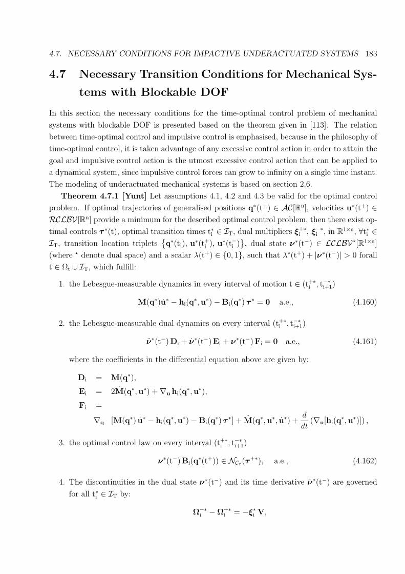
4.7. NECESSARY CONDITIONS FOR IMPACTIVE UNDERACTUATED SYSTEMS 183
4.7 Necessary Transition Conditions for Mechanical Sys-
tems with Blockable DOF
In this section the necessary conditions for the time-optimal control problem of mechanical
systems with blockable DOF is presented based on the theorem given in [113]. The relation
between time-optimal control and impulsive control is emphasised, because in the philosophy of
time-optimal control, it is taken advantage of any excessive control action in order to attain the
goal and impulsive control action is the utmost excessive control action that can be applied to
a dynamical system, since impulsive control forces can grow to infinity on a single time instant.
The modeling of underactuated mechanical systems is based on section 2.6.
Theorem 4.7.1 [Yunt] Let assumptions 4.1, 4.2 and 4.3 be valid for the optimal control
problem. If optimal trajectories of generalised positions q∗(t+) ∈ AC[Rn], velocities u∗(t+) ∈RCLBV [Rn] provide a minimum for the described optimal control problem, then there exist op-
timal controls τ ∗(t), optimal transition times t∗i ∈ IT, dual multipliers ξ+∗i , ξ−∗i , in R1×n, ∀t∗i ∈
IT, transition location tripletsq∗(ti), u∗(t+
i ), u∗(t−i ), dual state ν∗(t−) ∈ LCLBV?[R1×n]
(where ? denote dual space) and a scalar λ(t+) ∈ 0, 1, such that λ∗(t+) + |ν∗(t−)| > 0 forall
t ∈ Ωt ∪ IT, which fulfill:
1. the Lebesgue-measurable dynamics in every interval of motion t ∈ (t+∗i , t−∗i+1)
M(q∗)u∗ − hi(q∗,u∗)−Bi(q
∗) τ ∗ = 0 a.e., (4.160)
2. the Lebesgue-measurable dual dynamics on every interval (t+∗i , t−∗i+1)
ν∗(t−)Di + ν∗(t−)Ei + ν∗(t−)Fi = 0 a.e., (4.161)
where the coefficients in the differential equation above are given by:
Di = M(q∗),
Ei = 2M(q∗,u∗) +∇u hi(q∗,u∗),
Fi =
∇q [M(q∗) u∗ − hi(q∗,u∗)−Bi(q
∗) τ ∗] + M(q∗,u∗, u∗) +d
dt(∇u[hi(q
∗,u∗)]) ,
3. the optimal control law on every interval (t+∗i , t−∗i+1)
ν∗(t−)Bi(q∗(t+)) ∈ NCτ (τ
+∗), a.e., (4.162)
4. The discontinuities in the dual state ν∗(t−) and its time derivative ν∗(t−) are governed
for all t∗i ∈ IT by:
Ω−∗i −Ω+∗
i = −ξ∗i V,

184 CHAPTER 4. DISCONTINUOUS TRANSVERSALITY AND IMPULSIVE CONTROL
where ξ∗i = ξ+∗i + ξ−∗i , and
V =
[∇q
(WT
b u(t+i )
)
∇q
(WT
f u(t+i )
)−∇q
(Ku(t−i )
)]
. (4.163)
Further,(ν∗(t+
i )− ν∗(t−i ))
M(q(t)) = ξ∗i
[WT
b
Gfb G−1bb WT
b
], (4.164)
for some ξ+∗i , ξ−∗i ∈ Rn is necessary,
5. The jump in the generalised velocities shall fulfill:
u∗(t+i ) = P>
⊥(q∗(ti))u∗(t−i ), ∀t∗i ∈ IT. (4.165)
and
C∗Ti∩ C∗Ii =
q∗(ti)
u∗(t−i )
u∗(t+i )
∣∣∣∣∣∣∣L (q∗(ti))
[u∗(t+
i )
u∗(t−i )
]= 0
, ∀ t∗i ∈ IT.
with
L (q∗(ti)) =
[WT
b (q∗(ti)) 0
WTf (q∗(ti)) −K(q∗(ti))
], (4.166)
6. the condition for all t∗i ∈ IT
Υ+∗i + Υ−∗
i = ri1 u∗(t−i ) + ri2 u∗(t+i ) + ri3 u∗(t−i ) + ri4 u∗(t+
i ),
where the vectors ri1, ri2, ri3 and ri4 are given by:
r1 u∗(t−i ) + r2 u∗(t+i ) = V
(ξ−∗i u∗(t−i ) + ξ+∗
i u∗(t+i )
).
r3 = −ξ−∗i
[0
−K
], r4 = −ξ+∗
i
[WT
b
WTf
],
7. the boundary constraints Cf ,
8. the variational inequality with respect to the variations at final time tf :(Υ∗
f − 〈Ψ↑Cf (·; q(tf)), u∗(tf)〉 − 〈Ψ↑
Cf (·; u(tf)), u∗(tf〉)〉)
tf ≥ 0, ∀ tf ∈ R, (4.167)
9. the transversality condition at final state:[−Ω∗
f
−ν∗(tf)M
]∈ NCf (q∗(tf),u
∗(tf)) . (4.168)
Here Ωi and Υi are defined by
Ωi = −(ν(ti)M + ν(ti)M)− ν(ti)∇u(ti) hi,
Υi = −ν(ti) (∇u hi u(ti) + Mu(ti))−(ν(ti)M + ν(ti) M
)u(ti).

Chapter 5
Necessary Conditions in the
Hamiltonian Framework
The aim of this section is to derive an impulsive PMP by making use of the internal bound-
ary variations and discontinuous transversality conditions for finite-dimensional Lagrangian
systems. By the application of subdifferential calculus techniques to extended-valued lower
semi-continuous functionals, Pontryagin’s Maximum Principle (PMP) like conditions are ob-
tained. The considered functional is a generalized Bolza functional that is evaluated on multiple
intervals. The well-known PMP entails the necessary conditions for optimal control problems
with differential constraints and end-point constraints with sufficient regularity properties in
the space of absolutely continuous arcs (AC). However, impulsive optimal control requires to
search extremizing arcs in the space of bounded variation arcs (BV). So the obtained nec-
essary conditions encompasses PMP conditions under mild hypotheses since the class of BVarcs totally encompass the class of AC arcs. For the introduction to variational calculus with
elementary convexity considerations, the monograph of Troutman [101] recommended. For an
advanced introduction to the theory of subgradients and its applications to optimisation in
the nonconvex setting the monograph [88] is didactically suitable. A very good overview to
the application of nonsmooth analysis to control theory is given in the monograph [31]. The
monograph of Vinter [103] presents the up to date state of optimal control in the nonsmooth
setting. The main result in this chapter is presented and published in [110] by Yunt.
5.1 Derivation of Necessary Conditions in first-order form
In this section the necessary conditions for the optimal control problem of a structure-variant
mechanical system are derived. The specific problem considered has an impactive transition
at time ti, such that the structure of the equations of motion in the pre-transition and post-
transition phases may differ. In order to deal with the change of dimension of admissible
185

186 CHAPTER 5. HAMILTONIAN APPROACH
variations, the projective approach is used as discussed in subsection 2.6.2. A first-order rep-
resentation of mechanical dynamics is used in order to interpret the characteristics of the
investigated optimal control problem in the hamiltonian framework.
5.2 Generalised Problem of Bolza
Let us consider a problem in Bolza form (GPB), in which the objective is to choose an absolutely
continuous arc x ∈ AC in order to minimize
P : J(x) = l(x(a),x(b)) +
∫ b
a
L(t,x(t), x(t)) dt (5.1)
where the function L : [a, b] × Rn × Rn → R ∪ +∞ is L × B measurable. Here L × Bdenotes the σ-algebra of subsets of [a, b]× Rn generated by product sets M×N , where M is
a Lebesgue measurable subset of [a, b] and N is a Borel subset of R2 n. For each t ∈ [a, b], the
function l and L are lower semi-continuous (l.s.c) on Rn × Rn, with values in R ∪ +∞. For
each (t,x) in [a, b] × Rn, the function L(t,x, ·) is convex and l represents the endpoint cost.
GPB concerns the minimisation of a functional whose form is identical to that in the classical
calculus of variations. The GPB is distinguished from its classical version, by the extremely
mild hypotheses imposed on the endpoint cost l and the integrand L. Both are allowed to take
the value +∞. An important class of optimal control problems constrain the derivative of an
admissible arc and they can be stated as the following Mayer problem:
minl(x(a),x(b)) : x(t) ∈ F(t,x(t)), a.e. t ∈ [a, b]. (5.2)
The Mayer problem can be seen as minimizing the Bolza functional J over all arc x. To cover
the Mayer problem, it suffices to choose:
L(t,x,v) = ΨF(t,x)(v) =
0, if v ∈ F(t,x)
+∞, otherwise.(5.3)
The function ΨC is called the indicator function of the set C. It is evident that for any arc x,
one has ∫ b
a
L(t,x, x) dt =
0, if x(t) ∈ F(t,x) a.e.
+∞, otherwise.(5.4)
The Mayer type variational problem can arise from a typical dynamic constraint in controls
such as
x(t) = f(t,x(t), τ (t)), a.e. t ∈ [a, b], τ (t) ∈ Cτ . (5.5)
If a control state-pair (τ ,x) satisfies equation (5.5), then
x(t) ∈ F(t,x(t)) := f(t,x(t), τ (t)) : τ (t) ∈ Cτ a.e. t ∈ [a, b] (5.6)

5.2. GENERALISED PROBLEM OF BOLZA 187
certainly does. The well-known Fillipov’s theorem is the statement that the reversal of the
above statement is true.
In order to guarantee the well-behaving of F and l let following hypotheses hold:
Assumptions 5.2. An arc x : [a, b] → Rn is given. On some relatively open subset Ω ⊆[a, b]× Rn containing the graph of x, the following statements hold:
1. The multifunction F is L × B measurable on Ω. For each (t,x) in Ω, the set F(t,x) is
nonempty, compact and convex.
2. There are nonnegative integrable functions k and Φ on [a, b] such that
(a) F(t,x) ⊆ Φ(t)B for all x in Ωt, almost everywhere, and
(b) F(t,x) ⊆ F(t,x) + k(t)|y − x|clB for all x, y ∈ Ωt, almost everywhere.
3. The endpoint cost function l is l.s.c on Ωa × Ωb.
where Ωt = x ∈ Rn : (t,x) ∈ Ω for each t in [a, b] and B is the unit open ball.
The generalised problem of many practical problems place constraints not only on the derivative
of the state trajectory, but also on its endpoints. The differential inclusion problem is augmented
with the additional constraint (x(a),x(b)) ∈ S, where S is a given target set in Rn × Rn and
is assumed to be closed. Suppose that there is a function ϕ(t,x) with the following properties:
1. ϕ(t,x) ∈ F(t,x) for all x ∈ Ωt, almost everywhere;
2. ϕ(t,x) is a Caratheodory function, i.e., ϕ is L×B measurable on Ω, and for almost every
t the function x 7→ ϕ(t,x) is Lipschitz on Ωt with Lipschitz rank k(t);
3. ˙x(t) = ϕ(t, x(t)) almost everywhere on [a, b].
Given this setting the well-known PMP is stated in the formalism of nonsmooth analysis as
follows:
Theorem 5.1 -Pontryagin’s Maximum Principle Consider the optimal control problem
of minimizing the endpoint function
l(x(a),x(b)) + ΨS(x(a),x(b)) (5.7)
over all arcs x satisfying the differential constraint
x(t) = f(t,x(t), τ (t)), τ (t) ∈ Cτ , a.e. t ∈ [a, b]. (5.8)
In addition, suppose that f is a Caratheodory function for which the velocity sets F(t,x(t))
= v|v = f(t,x(t), τ (t)), τ (t) ∈ Cτ satisfy assumptions 5.2. If an arc x, together with a
corresponding control function τ , solves this problem, then there exist an arc p ∈ AC on [a, b]
and a scalar λ equal to either 0 or 1 for which one has, for almost every t ∈ [a, b],

188 CHAPTER 5. HAMILTONIAN APPROACH
• the adjoint equation,
−p(t) ∈ ∂x〈p(t), f(t, x(t), τ (t))〉, (5.9)
• the maximum condition
〈p(t), f(t, x, τ )〉 = sup〈p, f(t, x, τ )〉 : τ ∈ Cτ, (5.10)
• the transversality conditon
(p(a),−p(b)) ∈ λ ∂l(x(a), x(b)) +NS(x(a), x(b)). (5.11)
Here NS(x(a), x(b)) denotes the limiting normal cone to the set S at (x(a), x(b)). The operator
∂ denotes generalised subdifferential in the sense of Clarke. The above stated form of the
Pontryagin’s maximum principle (PMP) defines the necessary conditions for an arc x ∈ AC to
extremize the Mayer problem subject to the constraints S.
In the impulsive optimal control, it is assumed that the control horizon is composed of n
different phases, which are separated from each other by N − 1 possibly discontinuous transi-
tions. The importance of the transition process becomes clear if one considers the fact that
at pre-transition and post-transition states the values of several functions may differ due to
discontinuities. A transition process is common to the pre-transition configuration and post-
transition configuration. Each problem Pi with a unique mechanical configuration is defined on
a closed time domain dom(Pi) with variable boundary which is partitioned as follows:
dom(Pi) =t−i , t+
i
⋃ (, t+
i , t−i+1
) ⋃ t−i+1, t+
i+1
. (5.12)
The boundary of the domain dom(Pi) is given by:
bdy dom(Pi) =t−i , t+
i
⋃ t−i+1, t+
i+1
. (5.13)
The interior of the domain is given by:
int dom(Pi) =(t+i , t−i+1
). (5.14)
The domain of the overall problem PTot is given by the union:
dom(PTot) =⋃
∀ i
dom(Pi). (5.15)
However, the domains of successive problems Pi and Pi+1 are not disjoint:
dom(Pi)⋂
dom(Pi+1) = bdy dom(Pi)⋂
bdy dom(Pi+1) =t−i+1, t+
i+1
, (5.16)
The set bdy dom(Pi)⋂
bdy dom(Pi+1) =t−i+1, t+
i+1
is the support of the transition process
and is Lebesgue-negligible.

5.3. STATEMENT OF IOC 189
Having set the stage, the necessary conditions for the impulsive optimal control of structure-
variant rigid-body mechanical systems is formally derived by considering a problem in Bolza
form (GPB), in which the objective is to choose an arc x ∈ BV in order to minimize
J(x,x(t−i ), x(t+
i ), ti
) =
N∑i=1
li(x(t−i ),x(t+i )) +
∫ t−i+1
t+i
Li(t,x(t), x(t)) dt. (5.17)
The overall problem as stated in (5.17) is seen as the union of several problems in the gen-
eralised Bolza form. The theory at hand treats optimal solutions as solutions of multi-point
boundary value problems (MBVP) with discontinuous transitions in the state. In this setting,
the prespecification of the mode sequence and number of intervals must be given in advance.
Here it is assumed that the control horizon is composed of n different phases, which are sepa-
rated from each other by N− 1 possibly discontinuous transitions in the generalised velocities.
The extended-valued integrand may differ on each interval based on the structure of the equa-
tions of motion. The difference in structure may arise due to change in parameters ( i.e. mass,
inertia) or degrees of freedom. In [113] by Yunt a projection approach is presented in case,
the mechanical configurations in successive intervals differ based on change in the number of
degrees of freedom.
5.3 Impulsive Optimal Control Problem in First-Order
Form
The time-optimal control problem with free end-time tf and free transition times ti and location
q(ti), u(t−i ), u(t+i ) is considered. The assumptions during a possibly impactive transition are
given as follows:
Assumptions 5.2
1. The transitions may be impactively.
2. The generalised position remain unchanged during transition.
3. The impulsive control action acts on the system at a time instant ti which is Lebesgue-
negligible and there are countably many of such transition instants.
4. At a possibly impactive transition, the pre-transition controller configuration is assumed
to be effective.
5. There are no transitions at t0 and tf .
The necessary conditions are derived by making use of following assumptions on the general
problem:

190 CHAPTER 5. HAMILTONIAN APPROACH
Assumptions 5.3
1. the dual states η1 and η2 are assumed left-continuous locally bounded variation func-
tions (LCLBV), and the generalised velocities u of the Lagrangian system is assumed
right-continuous locally bounded variation functions (RCLBV), whereas the generalised
positions are in class AC.
2. The mode sequence and number of intervals for the MBVP constitute a feasible hybrid
trajectory.
3. The set C+Ii∩ C+
Tiis closed and nonempty.
4. The set C−Ii ∩ C−Tiis is closed and nonempty.
5. The goal functional g(q,y, τ ) is continuously differentiable forall t ∈ Ωt and ti ∈ IT.
6. The derivatives ∂yg(q,y, τ ) are bounded for all t ∈ Ωt and ti ∈ IT.
7. Each Li : (t+i , t−i+1)× Rn × Rn × Rn × Rn → R ∪ +∞ is a Lebesgue normal integrand.
8. Each Li(q(s),y(s), ·) is convex for each (q(s),y(s)).
9. Each li : Rn × Rn × Rn → R ∪ +∞ is lower semicontinuous.
The value function J has some pleasant regularity properties if assumptions 5.3 hold. Making
use of these regularity properties, ”sharp” necessary conditions are derived. The goal function
is given by:
min
∫ tf
t0
dt, (5.18)
subject to the mechanical system dynamics stated in the first-order measure-differential equa-
tion form:
dq = y dt, (5.19)
dy = (fi(q(t),y(t)) + Gi(q(t))τ (t)) dt + Vi(q(t))ζ ′ dσ. (5.20)
The smooth dynamics of the rigidbody mechanical system is characterised in every interval
of motion (t+i , t−i+1) by a triplet fi(q(t),y(t)),Gi(q(t)),Vi(q(t)). By the Lebesgue-Stieltjes
integration of equation (5.20) over an atom of time instant ti ∈ IT one obtains:
∫
tidy − (fi + Giτ (t)) dt−Viζ
′ dσ = y(t+i )− y(t−i )−Vi(q(ti))
(ζ+
i − ζ−i)
(5.21)
which is an impact equation in first order form. In performing the integration in (5.21), it is
assumed that the generalised impulsive control force directions Vi(q(ti)) do not change their

5.3. STATEMENT OF IOC 191
structure. In performing the integration in (5.21), it is assumed that the generalised impulsive
control force directions Vi(q(ti)) do not change their structure. The vector controls τ is assumed
to be constrained in a polytopic compact convex set denoted by Cτ . The overall value functional
is given by:
J = ΨCf +∑i∈IT
ΨC−Ti
+ ΨC+Ti
+
∫
(t0,tf)
ΨCτ dt + dH − 〈η1, dq〉 − 〈η2, dy〉 . (5.22)
The differential measure of the Hamiltonian is defined as:
dH = Ht dt + Hσ dσ = (5.23)
〈η2(t),Viζ′〉 dσ + (λ(t) g(q, y, τ ) + 〈η1(t), y(t)〉+ 〈η2(t), (fi + Giτ (t))〉 ) dt
where η1(t) ∈ LCBV?(R1×n) and η2(t) ∈ LCBV?(R1×n) are the dual states. The unconstrained
functional in (5.22) is equivalent to (5.24) under assumption 5.1.4:
J = ΨCf +∑i∈IT
ΨC−Ii+ ΨC+
Ii
+ ΨC−Ti
+ ΨC+Ti
+
∫ t−i+1
t+i
ΨCτ + Ht − 〈η1, u〉 − 〈η2, y〉 dt. (5.24)
Following structure for various differential measures is noted:
dq = u dt + ρ′ dσ, dy = q dt + χ′ dσ,
dη1 = η1 dt + ξ′1 dσ, dη2 = η2 dt + ξ′2 dσ.
The vector controls τ is assumed to be constrained in a polytopic convex set denoted by Cτ .
Here the sets are defined as below:
T +i =
q(t+
i ),u(t−i ),u(t+i )
|A1(q(t+i ))u(t−i ) + A2(q(t+
i ))u(t+i ) = 0
, (5.25)
T −i =
(q(t−i ),u(t−i ),u(t+
i ) |A1(q(t−i ))u(t−i ) + A2(q(t−i ))u(t+
i ) = 0
, (5.26)
Cf = q(tf),u(tf) |q(tf) = qf , u(tf) = uf , (5.27)
Cτ = τ |τ ∈ K, convex, polytopic , (5.28)
C+Ii
=
q(t+i ),y(t+
i ),y(t−i )∣∣ y(t+
i )− y(t−i )−Vi(q(t+i ))
(ζ+
i − ζ−i)
= 0
, (5.29)
C−Ii =
q(t−i ),y(t+i ),y(t−i )
∣∣ y(t+i )− y(t−i )−Vi(q(t−i ))
(ζ+
i − ζ−i)
= 0
. (5.30)
Here A1 and A2 are n × n dimensional linear operators. The set of transition conditions at
each transition instant ti are denoted by Ti, and are stated in terms of generalised positions
q(ti), and generalised post-, and pre-transition velocities u(t+i ), u(t−i ).
The directional derivatives of the augmented cost function in equation (5.24) is evalu-
ated with respect to q(t), y(t), ˆy(t), τ (t), q(tf), q(t+i ), q(t−i ), y(tf), y(t+
i ), y(t−i ), tf , t+i , t−i ,
ζ+
i , ζ−i . The directional derivative in direction q(t) is given by:
J↑(·, q(t)) =N−1∑i=0
∫ t−i+1
t+i
⟨∇q H i+1t , q(t)
⟩dt, ∀ t ∈ int dom(Pi). (5.31)

192 CHAPTER 5. HAMILTONIAN APPROACH
The directional derivative in direction y(t) is given by:
J↑(·, y(t)) =N−1∑i=0
∫ t−i+1
t+i
⟨∇y H i+1t , y(t)
⟩dt, ∀ t ∈ int dom(Pi). (5.32)
The directional derivative in direction u(t) is given by:
J↑(·, u(t)) = −N−1∑i=0
∫ t−i+1
t+i
〈η1(t), u(t)〉 dt, ∀ t ∈ int dom(Pi). (5.33)
The directional derivative in direction ˆy(t) is given by:
J↑(·, ˆy(t)) = −N−1∑i=0
∫ t−i+1
t+i
⟨η2(t), ˆy(t)
⟩dt, ∀ t ∈ int dom(Pi). (5.34)
The directional derivative in direction τ (t) is given by:
J↑(·, τ (t)) =N−1∑i=0
∫ t−i+1
t+i
⟨∇τ H i+1t , τ (t)
⟩+ Ψ↑
Cτ(·, τ (t)) dt, ∀ t ∈ int dom(Pi). (5.35)
The directional derivative in direction t−i at every ti ∈ IT is given by:
J↑(·, t−i ) =(H i
t(q(t−i ),y(t−i ))− ⟨η1(t
−i ), u(t−i )
⟩− ⟨η2(t
−i ), y(t−i )
⟩)t−i . (5.36)
The directional derivative in direction t+i at every ti ∈ IT is given by:
J↑(·, t+i ) = − (
H i+1t (q(t+
i ),y(t+i ))− ⟨
η1(t+i ), u(t+
i )⟩− ⟨
η2(t+i ), y(t+
i )⟩)
t+i . (5.37)
The directional derivative in direction tf at final time tf is given by:
J↑(·, tf) =(H i
t(q(tf),y(tf))− 〈η1(tf), u(tf)〉 − 〈η2(tf), y(tf)〉)
tf + ΨCf (·, tf). (5.38)
The directional derivatives of J in directions q(tf), q(t+i ), q(t−i ), y(tf), y(t+
i ), y(t−i ), ζ−i and
ζ+
i at every ti ∈ IT are given by:
J↑(·, q(t+i )) = Ψ↑
C+Ii
(·, q(t+i )) + Ψ↑
T +i
(·, q(t+i )), (5.39)
J↑(·, q(t−i )) = Ψ↑C−Ii
(·, q(t−i )) + Ψ↑T −i
(·, q(t−i )), (5.40)
J↑(·, y(t+i )) = Ψ↑
C−Ii(·, y(t+
i )) + Ψ↑C+Ii
(·, y(t+i )) + Ψ↑
T −i(·, y(t+
i )) + Ψ↑T +i
(·, y(t+i )),
(5.41)
J↑(·, y(t−i )) = Ψ↑C−Ii
(·, y(t−i )) + Ψ↑C+Ii
(·, y(t−i )) + Ψ↑T −i
(·, y(t−i )) + Ψ↑T +i
(·, y(t−i )),
(5.42)
J↑(·, ζ+
i ) = Ψ↑C+Ii
(·, ζ+
i ) + Ψ↑C−Ii
(·, ζ+
i ), (5.43)
J↑(·, ζ−i ) = Ψ↑
C+Ii
(·, ζ−i ) + Ψ↑
C−Ii(·, ζ
−i ), (5.44)
J↑(·, q(tf)) = Ψ↑Cf (·, q(tf)), (5.45)
J↑(·, y(tf)) = Ψ↑Cf (·, y(tf)), (5.46)

5.3. STATEMENT OF IOC 193
respectively. The directional derivatives of ΨC+Ii
in directions q(t+i ), y(t+
i ), y(t−i ), ζ−i and ζ
+
i at
every ti ∈ IT are given by:
Ψ↑C+Ii
(·, y(t−i )) = − ⟨λ+
i , y(t−i )⟩, (5.47)
Ψ↑C+Ii
(·, q(t+i )) =
⟨λ+
i , ∇qVi(q(t+i ))
(ζ+
i − ζ−i)
q(t+i )
⟩, (5.48)
Ψ↑C+Ii
(·, y(t+i )) =
⟨λ+
i , y(t+i )
⟩, (5.49)
Ψ↑C+Ii
(·, ζ+
i ) =⟨λ+
i , Vi(q(t+i )) ζ
+
i
⟩, (5.50)
Ψ↑C+Ii
(·, ζ−i ) = −
⟨λ+
i , Vi(q(t+i )) ζ
−i
⟩, (5.51)
respectively. The directional derivatives of ΨC−Iiin directions q(t−i ), y(t+
i ), y(t−i ), ζ−i and ζ
+
i at
every ti ∈ IT are given by:
Ψ↑C−Ii
(·, q(t−i )) =⟨λ−i , ∇qVi(q(t−i ))
(ζ+
i − ζ−i)
q(t−i )⟩, (5.52)
Ψ↑C−Ii
(·, y(t−i )) =⟨−λ−i , y(t−i )
⟩, (5.53)
Ψ↑C−Ii
(·, y(t+i )) =
⟨λ−i , y(t+
i )⟩, (5.54)
Ψ↑C−Ii
(·, ζ+
i ) =⟨
λ−i , Vi(q(t−i )) ζ+
i
⟩, (5.55)
Ψ↑C−Ii
(·, ζ−i ) =
⟨−λ−i , Vi(q(t−i )) ζ
−i
⟩, (5.56)
respectively. The directional derivatives of ΨT +i
in directions q(t+i ), y(t+
i ) and y(t−i ) at every
ti ∈ IT are given by:
Ψ↑T +i
(·, y(t−i )) =⟨ξ+
i , A1(q(t+i ))y(t−i )
⟩, (5.57)
Ψ↑T +i
(·, q(t+i )) =
⟨ξ+
i ,(∇qA1(q(t+
i ))y(t−i ) +∇qA2(q(t+i ))y(t+
i ))q(t+
i )⟩, (5.58)
Ψ↑T +i
(·, y(t+i )) =
⟨ξ+
i , A2(q(t+i ))y(t+
i )⟩. (5.59)
The directional derivatives of ΨT −i in directions q(t−i ), y(t+i ) and y(t−i ) at every ti ∈ IT are
given by:
Ψ↑T −i
(·, y(t−i )) =⟨ξ−i , A1(q(t−i ))y(t−i )
⟩, (5.60)
Ψ↑T −i
(·, q(t−i )) =⟨ξ−i ,
(∇qA1(q(t−i ))y(t−i ) +∇qA2(q(t−i ))y(t+i )
)q(t+
i )⟩, (5.61)
Ψ↑T −i
(·, y(t+i )) =
⟨ξ−i , A2(q(t−i ))y(t+
i )⟩. (5.62)
respectively.
The dual vectors λ+i , λ−i , ξ+
i and ξ−i are elements of Rn. By using the Lemma of Raymond-
Dubois in conjunction with proposition 2.1 the forms of equations (5.33) and (5.34) reveal on

194 CHAPTER 5. HAMILTONIAN APPROACH
very domain dom(Pi):
−∫ t−i+1
t+i
〈η1(t), u(t)〉 dt = −〈η1(t), q(t)〉 |t−i+1
t+i+
∫ t−i+1
t+i
〈η1(t), q(t)〉 dt, (5.63)
−∫ t−i+1
t+i
⟨η2(t), ˆy(t)
⟩dt = −〈η2(t), y(t)〉 |t
−i+1
t+i+
∫ t−i+1
t+i
〈η2(t), y(t)〉 dt, (5.64)
respectively. After the integrations the directional derivatives in direction q(t) and ˆq(t) can
be combined as in equation (5.65):
J↑(·, q(t)) =N−1∑i=0
∫ t−i+1
t+i
⟨(∇q H i+1
t + η1(t)), q(t)⟩
dt. (5.65)
Analogously, the directional derivatives in direction y(t) and ˆy(t) can be combined as in
equation (5.66):
J↑(·, y(t)) =N−1∑i=0
∫ t−i+1
t+i
⟨(∇y H i+1
t + η2(t)), y(t)⟩
dt. (5.66)
Further, the terms obtained by the directional derivatives q(tf), y(tf), q(t+i ) ,y(t+
i ), q(t−i ),
y(t−i ) can be brought in relation with the total variations qf , yf , q+i ,y+
i , q−i , y−i by the following
affine relations:
q(tf) = qf − u(tf) tf , (5.67)
y(tf) = yf − y(tf) tf , (5.68)
q(t+i ) = q+
i − u(t+i ) t+
i , (5.69)
y(t+i ) = y+
i − y(t+i ) t+
i − χ+i , (5.70)
q(t−i ) = q−i − u(t−i ) t−i , (5.71)
y(t−i ) = y−i − y(t−i ) t−i − χ−i , (5.72)
By making use of affine relations (5.67) to (5.72) the boundary variations are decomposed
into orthogonal independent variations in t−i , t+i , y+
i , y−i , q+i , q−i , ζ
−i , ζ
+
i at each transition
instant. Thus the internal boundary variations at each transition time are given in the finite-
dimensional set V :
V =
t−i , t+i , y+
i , y−i , q+i , q−i , ζ
+
i , ζ−i , χ−
i , χ+i
(5.73)
⊆ R× R× Rn × Rn × Rn × Rn × Rs × Rs × Rn × Rn.
The the internal boundary variations evaluated at transition time ti ∈ IT when recombined
with the forms obtained in (5.63) and (5.64) become:
⟨a1, q+
i
⟩+
⟨a2, q−i
⟩+
⟨a3, y+
i
⟩+
⟨a4, y−i
⟩+
⟨a5, t+
i
⟩+
⟨a6, t−i
⟩+
⟨a7, χ+
i
⟩+
⟨a8, χ−
i
⟩, (5.74)
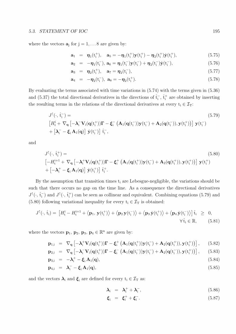
5.3. STATEMENT OF IOC 195
where the vectors aj for j = 1, . . . 8 are given by:
a1 = η1(t+i ), a5 = −η1(t
+i )y(t+
i )− η2(t+i )y(t+
i ), (5.75)
a2 = −η1(t−i ), a6 = η1(t
−i )y(t−i ) + η2(t
−i )y(t−i ), (5.76)
a3 = η2(t+i ), a7 = η2(t
−i ), (5.77)
a4 = −η2(t−i ), a8 = −η2(t
+i ). (5.78)
By evaluating the terms associated with time variations in (5.74) with the terms given in (5.36)
and (5.37) the total directional derivatives in the directions of t−i , t+i are obtained by inserting
the resulting terms in the relations of the directional derivatives at every ti ∈ IT:
J↑(·, t−i ) = (5.79)[H i
t + ∇q
[−λ−i Vi(q(t+i ))Γ− ξ−i
(A1(q(t−i ))y(t−i ) + A2(q(t−i )),y(t+
i ))]
y(t−i )
+[λ−i − ξi A1(q)
]y(t−i )
]t−i ,
and
J↑(·, t+i ) = (5.80)
[−H i+1t + ∇q
[−λ+i Vi(q(t+
i ))Γ− ξ+i
(A1(q(t+
i ))y(t−i ) + A2(q(t+i )),y(t+
i ))]
y(t+i )
+[−λ+
i − ξi A1(q)]
y(t+i )
]t+i .
By the assumption that transition times ti are Lebesgue-negligible, the variations should be
such that there occurs no gap on the time line. As a consequence the directional derivatives
J↑(·, t−i ) and J↑(·, t+i ) can be seen as collinear and equivalent. Combining equations (5.79) and
(5.80) following variational inequality for every ti ∈ IT is obtained:
J↑(·, ti) =[H i
t −H i+1t +
⟨p1, y(t+
i )⟩
+⟨p2 y(t−i )
⟩+
⟨p3 y(t+
i )⟩
+⟨p4 y(t−i )
⟩]ti ≥ 0,
∀ ti ∈ R, (5.81)
where the vectors p1, p2, p3, p4 ∈ Rn are given by:
p1,i = ∇q
[−λ+i Vi(q(t+
i ))Γ− ξ+i
(A1(q(t+
i ))y(t−i ) + A2(q(t+i )),y(t+
i ))]
, (5.82)
p2,i = ∇q
[−λ−i Vi(q(t+i ))Γ− ξ−i
(A1(q(t−i ))y(t−i ) + A2(q(t−i )),y(t+
i ))]
, (5.83)
p3,i = −λ+i − ξi A1(q), (5.84)
p4,i = λ−i − ξi A1(q), (5.85)
and the vectors λi and ξi are defined for every ti ∈ IT as:
λi = λ+i + λ−i , (5.86)
ξi = ξ+i + ξ−i . (5.87)

196 CHAPTER 5. HAMILTONIAN APPROACH
The directional derivatives of the value function J in directions ζ−i and ζ
+
i results in following
optimality conditions in variational inequality form at every ti ∈ IT:
J↑(·, ζ+
i ) =(λ+
i Vi(q(t+i )) + λ−i Vi(q(t−i ))
)ζ
+
i ≥ 0, ∀ ζ+
i ∈ Rr (5.88)
J↑(·, ζ−i ) = − (
λ+i Vi(q(t+
i )) + λ−i Vi(q(t−i )))
ζ−i ≥ 0, ∀ ζ
−i ∈ Rr. (5.89)
By the assumption that there are no discontinuities at a transition time ti in the generalised
positions q, the left and right total variations of the generalised positions q+i and q−i are taken
to be equal. The directional derivative of J in direction q+i is given by:
J↑(·, q+i ) =
[η1(t
+i ) + λ+
i ∇qVi
(ζ+
i − ζ−i)
+ ξ+i
(∇q A1 y(t+i ) +∇q A2 y(t−i )
)]q+
i ,
∀ q+i ∈ Rn. (5.90)
The directional derivative of J in direction q−i at every ti ∈ IT is given by:
J↑(·, q−i ) =[−η1(t
−i ) + λ−i ∇qVi
(ζ+
i − ζ−i)
+ ξ−i(∇q A1 y(t+
i ) +∇q A2 y(t−i ))]
q−i ,
∀ q−i ∈ Rn. (5.91)
By combining the equations (5.90) and (5.91) following variational inequality is obtained as
optimality condition for every ti ∈ IT:
J↑(·, qi) = (5.92)[η1(t
+i )− η1(t
−i ) + λi∇qVi
(ζ+
i − ζ−i)
+ ξi
(∇q A1 y(t+i ) +∇q A2 y(t−i )
)]qi ≥ 0,
∀ qi ∈ Rn.
The optimality conditions at final state are given as variational inequalities as as in inequal-
ities (5.93), (5.94) and (5.95) follows:
J↑(·, tf) = H it(q(tf),y(tf)) tf + Ψ↑
Cf (·, tf) ≥ 0, ∀ tf ∈ R, (5.93)
J↑(·, qf) = −η1(tf) qf + Ψ↑Cf (·, qf) ≥ 0, ∀ qf ∈ Rn, (5.94)
and
J↑(·, yf) = −η2(tf) yf + Ψ↑Cf (·, yf) ≥ 0, ∀ yf ∈ Rn. (5.95)
The directional derivatives with respect to χ+i and y+
i reveal the same expression as given
in (5.96) and (5.97) at every ti ∈ IT:
J↑(·, χ+i ) =
[−η2(t+i )− λi − ξi A2
]χ+
i ≥ 0, ∀ χ+i ∈ Rn. (5.96)
J↑(·, y+i ) =
[η2(t
+i ) + λi + ξi A2
]y+
i ≥ 0, ∀ y+i ∈ Rn. (5.97)

5.4. NECESSARY CONDITONS 197
The directional derivatives with respect to χ−i and y−i reveal the same expression as given
in (5.98) and (5.99) for every ti ∈ IT:
J↑(·, χ−i ) =
[η2(t
−i ) + λi − ξi A1
]χ−
i ≥ 0, ∀ χ−i ∈ Rn, (5.98)
J↑(·, y−i ) =[−η2(t
−i )− λi + ξi A1
]y−i ≥ 0, ∀ y−i ∈ Rn. (5.99)
in the respective intervals. The application of the variational inequality to conditions (5.66)
and (5.65) results in:
J↑(·, y(t)) =⟨(∇y H i
t + η2(t)), y(t)⟩ ≥ 0, a.e., ∀t ∈ (t+
i , t−i+1) ∈ IT,
∀ y(t) ∈ Rn (5.100)
and
J↑(·, q(t)) =⟨(∇q H i
t + η1(t)), q(t)⟩ ≥ 0, a.e., ∀t ∈ (t+
i , ti+1) ∈ IT,
∀ q(t) ∈ Rn. (5.101)
5.4 Necessary Conditions in First-Order Form
Theorem 5.2 [Yunt] Let assumptions 5.1, 5.2 and 5.3 be valid for the optimal control problem.
If trajectories of generalised positions q∗(t+) ∈ AC[Rn], velocities y∗(t+) ∈ RCLBV [Rn] provide
a minimum for the described optimal control problem, then there exist optimal transition times
t∗i ∈ IT, optimal controls τ ∗(t), optimal impulsive controls ζ−∗i , ζ+∗i , ∀ t∗i ∈ IT, dual multipliers
iξ+∗1 , iξ
−∗1 , iξ
+∗2 , iξ
−∗2 , α+∗
i , α−∗i , ∀t∗i ∈ IT, transition location triplets
q∗(ti), y∗(t+
i ), y∗(t−i ),
dual state η∗1(t−) ∈ LCLBV?[Rn] and η∗2(t
−) ∈ LCLBV?[Rn] (where ? denote dual space) and
a scalar λ(t) ∈ 0, 1, such that λ(t) + |ν| > 0, which fulfill:
• the dynamics of the mechanical system stated in first-order differential equation form:
u∗(t) = y∗(t), a.e., t ∈ (t+∗i , t−∗i+1), (5.102)
y∗(t) = fi(q∗(t),y∗(t)) + Gi(q
∗(t)) τ ∗, a.e., t ∈ (t+∗i , t−∗i+1), (5.103)
• the costate dynamics on the interior of of each subdomain int domPi of PT :
η∗1(t) = −∇q H = −∇qf(q∗(t),y∗(t)) +∇q g(q∗(t)) τ ∗(t))T η∗2(t), a.e.,(5.104)
η∗2(t) = −∇y H = −η∗1(t)− (∇y f(q∗(t),y∗(t)))Tη∗2(t), a.e., (5.105)
• The control constraints:
Cτ = τ |τ ∈ K, convex, polytopic . (5.106)

198 CHAPTER 5. HAMILTONIAN APPROACH
• The control law is given by:
−∇τ H it ∈ NCτ (τ
∗(t)), (5.107)
is fulfilled on the interior of of each subdomain int domPi of PT,
• The transition and impact conditions as given in sets (5.130), (5.131) ∀t∗i ∈ IT:
Ti =
q∗(ti)
y∗(t−i )
y∗(t+i )
∣∣A1(q∗(ti))u
∗(t−i ) + A2(q∗(ti)),u
∗(t+i ) = 0
, (5.108)
CIi =
q∗(ti)
y∗(t−i )
y∗(t+i )
∣∣y∗(t+i )− y∗(t−i )−Vi(q
∗(ti))(ζ+∗
i − ζ−∗i
)= 0
.
(5.109)
• the jump of the Lebesgue measurable part of the differential measure of the Hamiltonian:
H i+1t −H i
t =⟨pi1, y∗(t+
i )⟩
+⟨pi2, y∗(t−i )
⟩+
⟨pi3, y∗(t+
i )⟩
+⟨pi4, y∗(t−i )
⟩, (5.110)
∀ti ∈ IT,
where the vectors pi1, pi2, pi3 and pi1 are given by:
pi1 = ∇q
[−λ+∗i Vi(q
∗(t+i ))Γ∗ − ξ+∗
i
(A1(q
∗(t+i ))y∗(t−i ) + A2(q
∗(t+i )),y∗(t+
i ))]
,
pi2 = ∇q
[−λ−∗i Vi(q∗(t+
i ))Γ∗ − ξ−∗i
(A1(q
∗(t−i ))y∗(t−i ) + A2(q∗(t−i )),y∗(t+
i ))]
,
pi3 = −λ+∗i − ξ∗i A1(q
∗(t)),
pi4 = λ−∗i − ξ∗i A1(q∗(t)).
where ξ∗i = ξ+∗i + ξ−∗i .
• Further the vector λi is expected to fulfill:
λ∗i Vi(q∗(ti)) = 0, ∀t∗i ∈ IT. (5.111)
where λ∗i = λ+∗i + λ−∗i .
• The discontinuity condition of the dual state η1:
η∗1(t+i )− η∗1(t
−i ) = −λ∗i ∇q
[Vi
(ζ+∗
i − ζ−∗i
)]− ξ∗i ∇q
(A1 y∗(t+
i ) + A2 y∗(t−i )),
∀t∗i ∈ IT. (5.112)
The discontinuity condition of the dual state η2:
η∗2(t+i )− η∗2(t
−i ) = ξ∗i (A1(q
∗(ti))−A2(q∗(ti))) , ∀t∗i ∈ IT. (5.113)
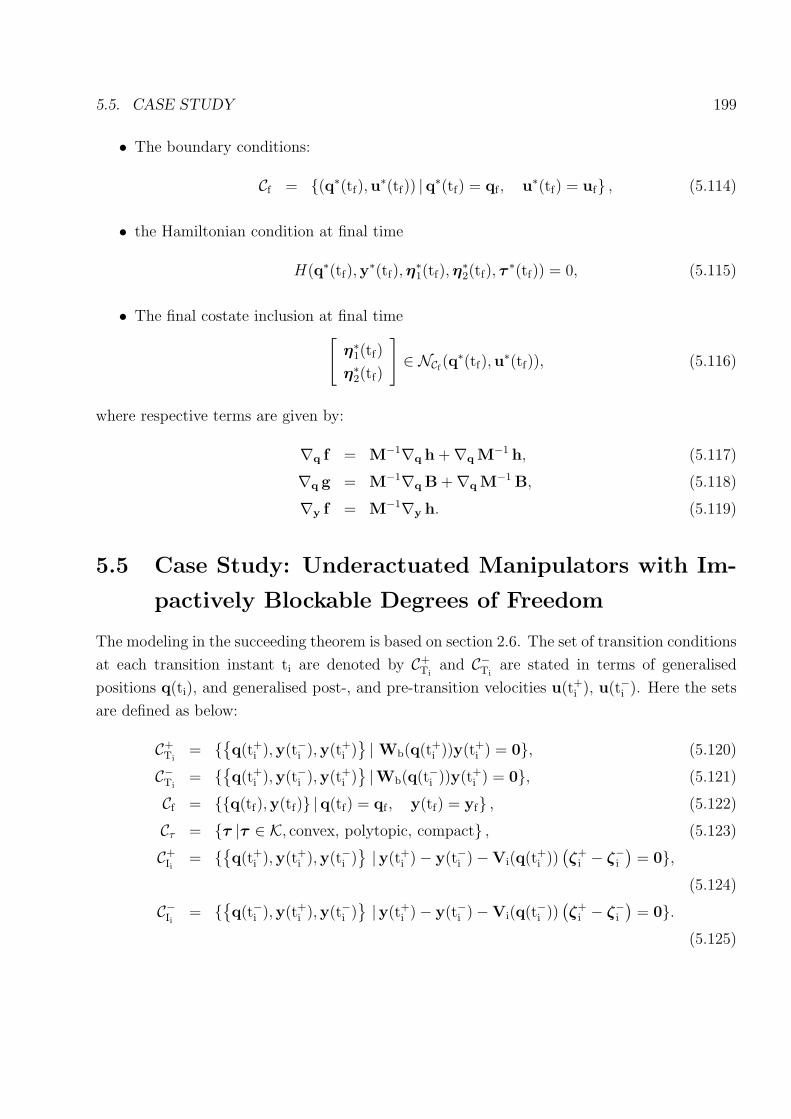
5.5. CASE STUDY 199
• The boundary conditions:
Cf = (q∗(tf),u∗(tf)) |q∗(tf) = qf , u∗(tf) = uf , (5.114)
• the Hamiltonian condition at final time
H(q∗(tf),y∗(tf),η
∗1(tf),η
∗2(tf), τ
∗(tf)) = 0, (5.115)
• The final costate inclusion at final time[
η∗1(tf)
η∗2(tf)
]∈ NCf (q
∗(tf),u∗(tf)), (5.116)
where respective terms are given by:
∇q f = M−1∇q h +∇q M−1 h, (5.117)
∇q g = M−1∇q B +∇q M−1 B, (5.118)
∇y f = M−1∇y h. (5.119)
5.5 Case Study: Underactuated Manipulators with Im-
pactively Blockable Degrees of Freedom
The modeling in the succeeding theorem is based on section 2.6. The set of transition conditions
at each transition instant ti are denoted by C+Ti
and C−Tiare stated in terms of generalised
positions q(ti), and generalised post-, and pre-transition velocities u(t+i ), u(t−i ). Here the sets
are defined as below:
C+Ti
= q(t+i ),y(t−i ),y(t+
i ) | Wb(q(t+
i ))y(t+i ) = 0, (5.120)
C−Ti= q(t+
i ),y(t−i ),y(t+i )
|Wb(q(t−i ))y(t+i ) = 0, (5.121)
Cf = q(tf),y(tf) |q(tf) = qf , y(tf) = yf , (5.122)
Cτ = τ |τ ∈ K, convex, polytopic, compact , (5.123)
C+Ii
= q(t+i ),y(t+
i ),y(t−i ) |y(t+
i )− y(t−i )−Vi(q(t+i ))
(ζ+
i − ζ−i)
= 0,(5.124)
C−Ii = q(t−i ),y(t+i ),y(t−i )
|y(t+i )− y(t−i )−Vi(q(t−i ))
(ζ+
i − ζ−i)
= 0.(5.125)

200 CHAPTER 5. HAMILTONIAN APPROACH
Theorem 5.3 [Yunt] Let assumptions 5.1, 5.2 and 5.3 be valid for the optimal control prob-
lem. If trajectories of generalised positions q∗(t+) ∈ AC[Rn], velocities y∗(t+) ∈ RCLBV [Rn]
provide a minimum for the described optimal control problem, then there exist optimal tran-
sition times t∗i ∈ IT, optimal controls τ ∗(t), optimal impulsive controls ζ+∗i − ζ−∗i , ∀ t∗i ∈ IT,
dual multipliers iξ+∗, iξ
−∗, ∀t∗i ∈ IT, transition location tripletsq∗(ti), y∗(t+
i ), y∗(t−i ), dual
states η∗1(t−) ∈ LCLBV?[R1×n] and η∗2(t
−) ∈ LCLBV?[R1×n] (where ? denote dual space) and
a scalar λ(t+) ∈ 0, 1, such that λ∗(t+) + |η∗1(t−)| + |η∗2(t−)| > 0 for all t ∈ Ωt ∪ IT, which
fulfill:
• the dynamics of the mechanical system stated in first-order differential equation form on
every interval t ∈ (t+∗i , t−∗i+1):
u∗(t) = y∗(t), a.e., (5.126)
y∗(t) = fi(q∗(t),y∗(t)) + Gi(q
∗(t)) τ ∗, a.e.
(5.127)
• the costate dynamics on every interval t ∈ (t+i , t−i+1):
η∗1(t) = −∇q H =
− ∇q (f(q∗(t),y∗(t)) + g(q∗(t)) τ ∗(t))T η∗2(t)− λ∗(t)∇q g(q∗(t),y∗(t), τ ∗(t)) a.e.,
(5.128)
η∗2(t) = −∇y H =
− η∗1(t)− (∇y f(q∗(t),y∗(t)))Tη∗2(t)− λ∗(t)∇y g(q∗(t),y∗(t), τ ∗(t)) a.e., (5.129)
• the control constraints Cτ which are convex and polytopic.
• the control law on ∀t ∈ (t+i , t−i+1) given by:
− ∇τ H it ∈ NCτ (τ
∗(t)),
• the transition and impact conditions as given in sets (5.130), (5.131) ∀t∗i ∈ IT:
C∗Ti= C∗Ti
+ ∪ C∗Ti
−, ∀t∗i ∈ IT (5.130)
C∗Ii = C∗Ii+ ∪ C∗Ii−, ∀t∗i ∈ IT, (5.131)
• the jump of the Lebesgue measurable part of the differential measure of the Hamiltonian:
H+∗t − H−∗
t = (5.132)
− ξ∗+i Ω∗i y∗(t+
i )− ξ∗−i Ω∗i y∗(t−i )− ξ∗i
([WT
b (q∗) 0
WTf (q∗) −K(q∗)
] [y∗(t+
i )
y∗(t−i )
]),

5.5. CASE STUDY 201
where Ω∗i is given by:
Ω∗i = ∇q
([WT
b (q∗) 0
WTf (q∗) −K(q∗)
] [y∗(t+
i )
y∗(t−i )
])
and ξ∗i ∈ R1×n by ξ∗i = ξ+∗i + ξ−∗i ,
• the discontinuities in η1 and η2 must fulfill:
η∗1(t+i )− η∗1(t
−i ) = −ξ∗i Ω∗
i (5.133)
and
η∗2(t+i )− η∗2(t
−i ) = −ξ∗i
[WT
b (q∗(ti))
Gfb(q∗(ti))G
−1bb (q∗(ti))W
Tb (q∗(ti))
], (5.134)
• the boundary conditions:
Cf =
(q∗(tf)
u∗(tf)
)|q∗(tf) = qf , u∗(tf) = uf
,
(5.135)
• the Hamiltonian condition at final time
Ht(q∗(tf),y
∗(tf), η∗1(tf),η
∗2(tf), τ
∗(tf)) = 0, (5.136)
• the transversality condition at final state:
[η∗1(tf)
η∗2(tf)
]∈ NCf (q
∗(tf),u∗(tf)). (5.137)

202 CHAPTER 5. HAMILTONIAN APPROACH
.

Chapter 6
Discussion and Conclusion
6.1 Results on Numerical Methods
The sweeping discretisation method has been since its introduction in the late sixties inves-
tigated intensively as an integration routine. The existence of switching control forces in the
distributional sense, implies that the transition indeed happen on a time-instant of Lebesgue
measure zero if one considers the continuous description of the problem, on the other side in the
discretisation it means that the transition happens on a discrete time interval on which the dis-
cretised differential measures of control forces exist in the distributional sense. The continuous
description is compliant to various hybrid system modeling approaches where transitions happen
on a time instant of Lebesgue-measure zero, whereas in the discretised treatment the problem
enables the transition to take place on a time interval of length of the discretisation length. In
literature there are several streams that treat in detail transitions on intervals with non-zero
Lebesgue measure in order to emulate physical reality and deny conventional hybrid system
descriptions by making use of examples from the physical world. The measure-differential in-
clusion approach and the sweeping discretisation comply in the continuous description with
conventional hybrid system modeling approaches which are reasonable, whereas the discretised
treatment accepts transitions on intervals. So by choosing minimum or maximum of the dis-
cretisation step length it is possible to limit transitions such that they comply with the physical
system which is investigated. In the opinion of the author, therefore it makes less sense to use
sweeping discretisation if the aim is to achieve numerical accuracy in the contact state transi-
tions because of the existence of contact forces in the distributional sense, and it recommends
itself to revert to event-driven integration schemes, whereas in order to obtain basically a robust
treatment of a fairly complex dynamical process sweeping discretisation scheme is superior in
providing quantitative data on the problem that compensates for the loss in the numerical ac-
curacy. Choosing a discretisation step length which is much smaller then any fast process that
takes place in the real system under consideration does not provide further information and
203

204 CHAPTER 6. DISCUSSION AND CONCLUSION
may complicate the numerical execution. In chapter two, aspect of modeling hybrid mechanical
systems is introduced and discussed. The necessity to represent FDL systems as MDI’s em-
anates from several facts. The optimal control of hybrid finite-dimensional Lagrangian systems
benefits from several aspects of the MDI approach, which are summarised below:
a The index sets that are used to take account of the behaviour of contacts on different levels
such as position, velocity and acceleration for stick-slip transitions etc. are not manage-
able for large systems with many contacts easily. The annihilation of the acceleration
level in the discretised form of the MDI removes the necessity to evaluate the status of
contacts on acceleration level. The index-set reduction can be seen in going from the
acceleration level representation in (2.40) to the measure-differential MDI representation
in (2.46).
b The impacts, that may occur with or without collisions like in the cases of the Painleve
Paradox, velocity jumps due to C0 constraints are a strong incentive to describe the
mechanical systems as MDI, because impacts may occur in the absence of impulsive force
action on the system and the MDI framework still captures the jump in the velocity in
these cases.
c Systems which are zeno (e.g jumping ball on the ground) are problematic for event-driven
schemes whereas MDI approach can handle them in its discretised form. In case of
infinitely many impulsive actions on the system in finite time, the discretisation scheme
by the choice of a minimum resolution induces a truncation of the infinite series and treats
the sum of all impacts as a single impact over a discretisation time step.
d The hybrid optimal control requires the consideration of an uncommon concept of control,
namely, controls of unbounded, impulsive and set-valued type for non-autonomous impul-
sive transitions, such as sudden blocking of DOF, which can in a natural way be embedded
into the MDI structure as discussed in sections 2.4 and 2.5.
e As a novel property, the location and time of phase transitions where the system changes
DOF is not prespecified but is determined as an outcome of the optimisation. Though
the underlying system might undergo structure-variant phase changes such as impactive
phase transitions a mixed integer approach is not necessary. This is due to the fact that in
this modeling framework every instant is equipped with the means to become a transition
instant for some classes of dynamical systems.
f Numerical methods can be deviced that calculate the costate dynamics which itself is de-
scribed as a MDI. The costate dynamics in the sense of optimal control is discontinuous
and nonsmooth, as presented in [115] in the sense of optimal control. So the evolution of

6.1. RESULTS ON NUMERICAL METHODS 205
the costate dynamics benefits from the same advantages of the MDI representation like
the mechanical dynamics itself.
Numerically, two methods have been presented, namely, one shooting method and one
nonlinear programming method. The nonlinear programming method has been developed with
the intention to localise the global minimum of the problem. The optimisation problem at hand,
is highly nonconvex, nonsmooth and the solution is generally non-unique. The non-uniqueness
of the solution arises due to the fact that the discretised differential of the normal control force
is unbounded and set-valued in the regions of transition. The non-smoothness arises due to the
non-differentiability of the Fischer-Burmeister function at the origin as depicted in figures 3.2
and 3.3 . The nonfavourable character of the optimisation problem in general and the general
coexistence of all these complications at the solution in the special render it very difficult
to obtain the global solution straightforward. However, the presented scheme is capable to
obtain a quasi-optimal solution near the optimal solution relatively easily. In obtaining the
global time-optimal solution, starting from a quasi-optimal solution the upper constrained on
final time is reduced sequentially at final stages of the optimisation and it is made use of the
global behaviour of the augmented Lagrangian method. In order to tackle the problem of
non-convexity the continuation parameter as shown in the flowchart in figure 3.6 is useful in
obtaining the quasi-optimal solution. The method is classified as a subgradient (Kiev) method
in solving nonsmooth optimisation problems. As one of the drawbacks of the method, it is
recognised that a termination criterion based on the norm of the gradient does not exist due to
the nonsmoothness. The utilisation of an augmented Lagrangian based subgradient method has
the advantage that another type of termination criterion is provided. A characteristic property
of the augmented Lagrangian method is the fact that the duality gap is also removed in the
nonconvex case if a pair of primal dual solutions exists. In the augmented Lagrangian scheme
described in section 3.3; the equality of the values of the primal and dual problems as stated in
equation (3.94) is used as termination criterion . This termination criterion provides a remedy
for the problem of the termination criterion of subgradient methods. Another property of the
augmented Lagrangian is the global behaviour of the scheme as discussed in subsection 3.2.4. By
the property of the convexification of the feasible region, the minimisation of the unconstrained
augmented Lagrangian method guarantees the convergence to an at least locally minimum if
the Slater condition is fulfilled. Numerically, solutions with discontinuities in the generalised
velocities evolve as the end time constraint approaches the optimal minimum time, i.e. given
enough time transitions become non-impactive and the scheme determines trajectories where
the underactuated is blocked, when the relative joint velocity is already zero. The ordinary
Lebesgue-measurable controls τ take the shape of bang-bang controls as shown in figures 3.11,
3.21 and 3.31, which indicates that a time-optimal solution is obtained. The evolution of the
generalised position and velocities are shown in the figures 3.9, 3.19 and 3.29 with clearly visible
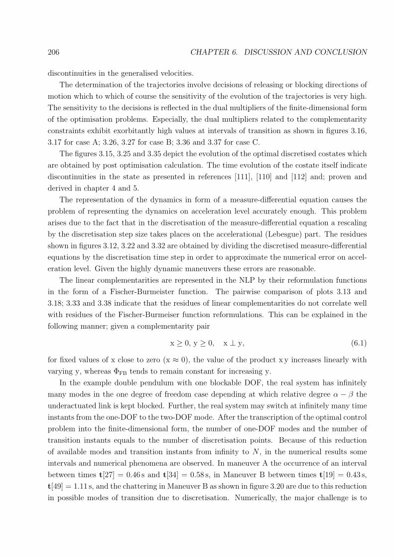
206 CHAPTER 6. DISCUSSION AND CONCLUSION
discontinuities in the generalised velocities.
The determination of the trajectories involve decisions of releasing or blocking directions of
motion which to which of course the sensitivity of the evolution of the trajectories is very high.
The sensitivity to the decisions is reflected in the dual multipliers of the finite-dimensional form
of the optimisation problems. Especially, the dual multipliers related to the complementarity
constraints exhibit exorbitantly high values at intervals of transition as shown in figures 3.16,
3.17 for case A; 3.26, 3.27 for case B; 3.36 and 3.37 for case C.
The figures 3.15, 3.25 and 3.35 depict the evolution of the optimal discretised costates which
are obtained by post optimisation calculation. The time evolution of the costate itself indicate
discontinuities in the state as presented in references [111], [110] and [112] and; proven and
derived in chapter 4 and 5.
The representation of the dynamics in form of a measure-differential equation causes the
problem of representing the dynamics on acceleration level accurately enough. This problem
arises due to the fact that in the discretisation of the measure-differential equation a rescaling
by the discretisation step size takes places on the accelerational (Lebesgue) part. The residues
shown in figures 3.12, 3.22 and 3.32 are obtained by dividing the discretised measure-differential
equations by the discretisation time step in order to approximate the numerical error on accel-
eration level. Given the highly dynamic maneuvers these errors are reasonable.
The linear complementarities are represented in the NLP by their reformulation functions
in the form of a Fischer-Burmeister function. The pairwise comparison of plots 3.13 and
3.18; 3.33 and 3.38 indicate that the residues of linear complementarities do not correlate well
with residues of the Fischer-Burmeiser function reformulations. This can be explained in the
following manner; given a complementarity pair
x ≥ 0, y ≥ 0, x ⊥ y, (6.1)
for fixed values of x close to zero (x ≈ 0), the value of the product x y increases linearly with
varying y, whereas ΦFB tends to remain constant for increasing y.
In the example double pendulum with one blockable DOF, the real system has infinitely
many modes in the one degree of freedom case depending at which relative degree α − β the
underactuated link is kept blocked. Further, the real system may switch at infinitely many time
instants from the one-DOF to the two-DOF mode. After the transcription of the optimal control
problem into the finite-dimensional form, the number of one-DOF modes and the number of
transition instants equals to the number of discretisation points. Because of this reduction
of available modes and transition instants from infinity to N , in the numerical results some
intervals and numerical phenomena are observed. In maneuver A the occurrence of an interval
between times t[27] = 0.46 s and t[34] = 0.58 s, in Maneuver B between times t[19] = 0.43 s,
t[49] = 1.11 s, and the chattering in Maneuver B as shown in figure 3.20 are due to this reduction
in possible modes of transition due to discretisation. Numerically, the major challenge is to

6.1. RESULTS ON NUMERICAL METHODS 207
investigate the stability of the optimal trajectories with respect to the discretisation scheme.
The investigation of general hybrid systems with respect to discretisation schemes is obviously
much harder. A common observation is that there is a threshold on the discretisation step
length below which the stability of the optimal trajectories is maintained, if the hybrid system
does not exhibit zeno behaviour.
A shooting method is presented for the determination of optimal trajectories for switching
Lagrangian systems and is applied to a highly nonlinear and nonsmooth system with variable
structure. The differential-drive robot is modeled in detail and the optimisation algorithm has
been detailed in order to provide a benchmark problem for further optimisation problems that
deal with the trajectory optimisation problem of switching Lagrangian systems. The advantage
of using sweeping discretisation in the trajectory optimisation problem is the qualitative advan-
tages it offers with respect to other optimisation approaches. By treating the contact forces and
the forces that induce transition as impulsive forces in the distributional sense, one obtains in
some cases the mode sequence and optimal transition instants and locations in advance without
prespecifying them. This is due to the fact that in this modeling framework every instant is
equipped with the means to become a transition instant. The event-driven nature of the opti-
misation problem is circumvented, by considering each discretisation time point as a possible
transition time where the system changes from one element to any another element in IM. The
resulting novel feature is that contrary to other shooting schemes for optimisation problems
with different phases, characterized by different system dynamics, multiple shooting is not nec-
essary. The proposed optimisation scheme determines over all possible hybrid executions that
lead to the final destination of switching Lagrangian system an at least locally-optimal solution.
As a consequence, the location and time of phase transitions where the system changes DOF
is not pre-specified but is determined as an outcome of the optimisation. The deficiency in
the energy balance can be considered as a price in order to obtain this important qualitative
informations by sacrifying some quantitative properties such as accuracy due deficiency in the
energy balance or low-order integration procedure. The main features of the sweeping based
direct shooting method combined with augmented Lagrangian is summarised as follows:
1 Though the underlying system might undergo structure-variant phase changes such as stick-
slip transitions multiple shooting is not necessary and a single shooting performs the
task.
2 Knowledge regarding adjoint variables is not necessary.
3 The method enables to obtain locally or globally optimal trajectories to switching Lagrangian
systems in a reduced search space in comparison to nonlinear programming methods where
total discretisation is necessary.

208 CHAPTER 6. DISCUSSION AND CONCLUSION
4 The sufficiency condition for a convergence to an at-least locally optimal solution is the
existence of a nonempty feasible set as discussed in [109].
5 The method minimizes over modes as well, and chooses a sequence of modes and transitions
which possess a certificate of optimality as presented in [109].
The global convergence of the combined direct shooting and augmented Lagrangian for solv-
ing the underlying problem is enhanced by the convexification induced by utilizing augmented
Lagrangian based optimisation. The minimisation strategy, that relies on combining the aug-
mented Lagrangian method with a nongradient simplex minimisation method profits from the
properties of the approaches that mutually complete each other:
• One of the main advantages of direct-search methods is that the minimisation is performed
by function value comparison, so that the problems of ill-conditioning due to high penalty
parameters that degrade the performance of methods that use first and second-order
information, is not a problem for such methods.
• The choice of a high penalty value has generally a convexifying effect. In this respect
direct methods are more suitable for a general class of optimisation problems. Direct
search methods have the disadvantage that their convergence in the vicinity of the solution
is slow. A partial remedy to this problem in the framework of the augmented Lagrangian
technique is the partial/incomplete minimisation approach in the intermediate stages of
the successive minimisations as discussed in [14].
• The local convexification of the feasible region, that is induced by the penalisation, guar-
antees that the unconstrained function is bounded-below and that through direct-search
methods the ¡feasible region is reached, even if the initial starting point of the optimisation
y0 is infeasible.
6.2 Variational Results
In this work, necessary conditions of strong local minimizers for the impulsive optimal control
problem of finite-dimensional Lagrangian systems is presented. The necessary conditions pro-
vide criteria for the determination of optimal transition times and locations in the presence of
discontinuity of generalised velocities. In the proposed setting concurrent discontinuity on an
Lebesgue-negligible time instant of the generalised velocities q and the dual state ν is handled.
The proposed discontinuous transversality conditions and the internal boundary variations by
the author are capable, given the assumptions in the statement of the optimal control problem,
to handle this problem properly. It is shown that the idea of internal boundary variations is in-
deed a natural extension of the classical boundary variations, where the latter one is unilateral

6.2. VARIATIONAL RESULTS 209
and the extension is a bilateral concept. In this work, a characterisation of these concepts in
terms of subderivatives to the extended-valued lower-semicontinuous directionally Lipschitzian
value functional is given, showing that these variational principles are, given certain regularity
assumptions, well founded in subdifferential calculus rather than being some ad-hoc assump-
tions. This capability is, in comparison to other impulsive control necessary conditions, far
more consistent with different hybrid system modeling approaches in which transitions happen
instantaneously. The proposed discontinuous transversality conditions and the internal bound-
ary variations by the author are capable, given the assumptions in the statement of the optimal
control problem, to handle this problem properly.
The derivation of conditions benefit of the underlying Lagrangian structure. One of the
advantages of the Lagrangian dynamics is the fact, that the generalised directions of control,
which are the rows of the linear operator B are only dependent on the generalised positions
q. Since the generalised positions are of absolutely continuous character, the generalised direc-
tions of impulsive control remain unchanged during a transition. Another fact is that in the
framework of finite-dimensional Lagrangian systems, impact equations and constitutive impact
laws are provided, that are means to ”join” two optimal trajectories discontinuously. Theorem
4.6.2 reflects the application of theorem 4.6.1 to underactuated manipulators with impactively
blockable degrees of free.
The proposed necessary conditions are for strong local minimizers and are valid in singular
intervals. The optimal control law as stated in equation (4.152) is valid in singular intervals,
because the zero vector belongs to normal cone. The discontinuity in the controls of bang-bang
type controller are on Lebesgue negligible intervals so the control law is valid in the ”almost
everywhere” sense.
The bang-bang control law can be affected at a transition due to two effects, which may
concur:
• The change in the structure of the Lebesgue-measurable dynamics as discussed in sub-
section 2.6.2, may induce a switching of the polarity of a bang-bang controller.
• The discontinuity of the generalised velocities and the dual state may result in a change
of the polarity after impulsive control action.
There are two sets of necessary conditions that belong to the considered optimal control
problem. The first set of necessary conditions are obtained by taking the generalised positions
and velocities as RCLBV functions and the dual state as a LCLBV function. The second set of
necessary conditions is obtained interchanging the classes of primal states q(t),u(t) and dual
state ν(t). In the case of state-continuous transitions, these two sets of necessary conditions
would coincide. Indeed, what distinguishes the necessary conditions stated in Theorem 4.6.1
from its counterpart if all transitions were state-continuous are the conditions (4.153), (4.155)

210 CHAPTER 6. DISCUSSION AND CONCLUSION
and (4.156). These conditions are derived by allowing variations in the post-transition and pre-
transition states along with impact equations and constitutive impact laws. Impulsive control
law in (4.157) takes this particular form because the impulsive controls are unbounded in this
setting.
Transition sets for discontinuities in the generalised velocities of mechanical systems are first
introduced in [112]. In this work, the properties of the transition sets are discussed, especially
from the viewpoint of regularity. For the underlying non-convex problem the given conditions
can only propose the candidates for minimizers, for the conditions of sufficiency further work
needs to conducted.
In chapter 5, necessary conditions of strong local minimizers for the impulsive optimal con-
trol problem of Lagrangian systems is presented, which are represented in first-order differential
equation form. The main result is theorem 5.2. Theorem 5.3 reflects the application of theorem
5.2 to underactuated manipulators with impactively blockable degrees of free. The treatment of
the impulsive-optimal control problem in this framework enables the analysis of the various fea-
tures in the Hamiltonian framework. This form of the representation of the problem is already
published in [110] and gives access to a broader class of dynamical systems. In this chapter the
necessary conditions are derived in detail and the necessary conditions are stated in a theorem.
As a case study, the necessary conditions for the impulsive optimal control of underactuated
manipulators with impulsively blockable DOF is presented. This equation indicates that under
the given hypotheses, the hamiltonian may only jump if a discontinuity in the generalised ve-
locities of the Lagrangian system occur. The necessary conditions for the time-optimal control
of underactuated manipulators with blockable DOF is stated in a first-order system setting.

Bibliography
211

Bibliography
[1] V. Acary, B. Brogliato, and D. Goeleven. Higher order moreau’s sweeping process: math-
ematical formulation and numerical simulation. Math. Program., Ser. A, 2006.
[2] N. U. Ahmed. Necessary conditions of optimality for impulsive systems on banach spaces.
Nonlinear Analysis, 51:409–424, 2002.
[3] N. U. Ahmed. Existence of optimal controls for a general class of impulsive systems on
banach spaces. SIAM J. Control Optim., 42(2):669–685, 2003.
[4] N. U. Ahmed. Measure solutions for evolution equations with discontinuous vector fields
and their optimal control. Nonlinear Analysis, 63:e33–e42, 2005.
[5] N. U. Ahmed. Measure solutions for impulsive evolution equations with measurable vector
fields. Mathematical Analysis and Applications, 319:74–93, 2006.
[6] P. Alart and A. Curnier. A mixed formulation for frictional contact problems prone to
newton like solution methods. Computer Methods in Applied Mechanics and Engineering,
92(3):353–375, 1991.
[7] M. Anitescu and A. P. Florian. A time-stepping method for stiff multibody dynamics
with contact and friction. Int. Journal for Num. Meth. in Engr., 55:753–784, 2001.
[8] A. Arutyunov, D. Karamzin, and F. Pereira. A nondegenerate maximum principle for
impulse control problem with state constraints. SIAM J. Control Optim., 43:1812–1843,
2005.
[9] D. J. Balkcom and M. Mason. Extremal trajectories for bounded velocity mobile robots.
In Proceedings of the 2002 IEEE International Conference on Robotics and Automation,
2002.
[10] A. Bemporad and M. Morari. Control of systems integrating logic, dynamic, and con-
straints. Automatica, 35:407–427, 1999.
212

BIBLIOGRAPHY 213
[11] S. C. Bengea and R. A. DeCarlo. Optimal control of switching systems. Automatica,
41:11–27, 2005.
[12] A. Bensoussan. Optimal impulsive control theory. In Stochastic Control Theory and
Stochastic Differential Systems, volume 16 of Lecture Notes in Control and Information
Sciences, pages 17–41. Springer, 1979.
[13] J. Bentsman, B. M. Miller, Rubinovich E. Y., and K. Zheng. Hybrid dynamical systems
with controlled discrete transitions. Nonlinear Analysis: Hybrid Systems, 1(4):466–481,
2007.
[14] D. Bertsekas. Nonlinear Programming, volume 4 of Optimisation and Computation Series.
Athena Scientific, 1999.
[15] J. T. Betts. Survey of numerical methods for trajectory optimisation. Journal of Guid-
ance, Control and Dynamics, 21(2):193–207, 1998.
[16] F. Borelli, M. Baotic, A. Bemporad, and M. Morari. Dynamic programming for con-
strained optimal control of discrete-time linear hybrid systems. Automatica, 41:1709–
1721, 2005.
[17] V. S. Branicky, M. S.and Borkar and S. M. Mitter. A unified framework for hybrid control:
Model and optimal theory. IEEE Transactions on Automatic Control, 43:31–45, 1998.
[18] A. Bressan. Impulsive control of lagrangian systems and locomotion in fluids. Journal of
Discrete and Continuous Dynamical Systems, 20(1):1–35, 2008.
[19] B. Brogliato. Nonsmooth Mechanics: Models, Dynamics and Control. Communications
and Control Engineering. Springer, 2nd edition, 1999.
[20] B. Brogliato. Some results on the optimal control with unilateral state constraints. Re-
search Report 5992, INRIA, 2006.
[21] B. Brogliato, A. Daniilidis, C. Lemarechal, and V. Acary. On the equivalence between
complementarity systems, projected systems and differential inclusions. Systems and
Control Letters, 55:45–51, 2006.
[22] C. Buskens and H. Maurer. Sqp-methods for solving optimal control problems with
control and state constraints: adjoint variables, sensitivity analysis and real-time control.
Journal of Computational and Applied Mathematics, 120:85–108, 2000.
[23] F.H. Clarke. The euler-lagrange differential inclusion. J. of Differential Equations, 19:80–
90, 1975.

214 BIBLIOGRAPHY
[24] F.H. Clarke. Calculus of Variations and Control Theory, chapter Necessary Conditions
for a General Control Problem, pages 257–278. Academic Press, 1976.
[25] F.H. Clarke. The generalised problem of bolza. SIAM J. Control and Optimisation,
14(4):682–698, 1976.
[26] F.H. Clarke. The maximum principle under minimal hypotheses. SIAM J. Control and
Optimisation, 14(6):1078–1091, 1976.
[27] F.H. Clarke. A new approach to lagrange multipliers. Mathematics of Operations Re-
search, 1(2):165–174, 1976.
[28] F.H. Clarke. Extremal arcs and extended hamiltonian systems. Trans. of the Amer.
Math. Soc., 1977.
[29] F.H. Clarke. Optimisation and Nonsmooth Analysis. Number 5 in Classics in Applied
Mathematics. SIAM, 1990.
[30] F.H. Clarke and C. Nour. Nonconvex duality in optimal control. SIAM J. Control Optim.,
43(6):2036–2048, 2005.
[31] F.H. Clarke, Ledyaev Yu.S., Stern R.J., and Wolenski P.R. Nonsmooth Analysis and
Control Theory. Number 178 in Graduate Texts in Mathematics. Springer, 1998.
[32] R. Cottle, W. Pang, and R. E. Stone. The Linear Complementarity Problem. Academic
Press Inc., 1992.
[33] M. Egerstedt, Y. Wardi, and H. Axelsson. Transition-time optimisation for switched-
mode dynamical systems. IEEE Trans. in Automatic Control, 51(1):110–115, 2006.
[34] M. Egerstedt, Y. Wardi, and F. Delmotte. Optimal control of switching times. In IEEE
Conference on Decision and Control, 2003.
[35] A. F. Fillipov. Differential equations with discontinuous right-hand side. American Math-
ematical Society Translations, 42:199–231, 1964.
[36] A. F. Fillipov. Classical solutions of differential equations with multivalued right-hand
side. SIAM J. Control Optim., 5:609–621, 1967.
[37] A. F. Fillipov. Differential Equations with Discontinuous Right-Hand Side. Kluwer Aca-
demic, 1988.
[38] A. Fischer. A special newton-type optimisation method. Optimisation, 24:269–284, 1992.

BIBLIOGRAPHY 215
[39] M. Fukushima and L. Qi, editors. Reformulation- Nonsmooth, Piecewise Smooth, Semis-
mooth and Smoothing Methods. Kluwer Academic Publishers, 1998.
[40] G. Galbraith and R. B. Vinter. Optimal control of hybrid systems with an infinite number
of discrete states. Journal of Dynamical and Control Systems, 9(4):563–584, 2003.
[41] A. A. Galyaev, B. M. Miller, and E. Y. Rubinovich. Analysis and Simulation of Contact
Problems, volume 27 of Lecture Notes in Applied and Computational Mechanics, pages
385–386. Springer, 2006.
[42] Ch. Glocker. Dynamik von Starrkorpersystemen mit Reibung und Stossen. PhD thesis,
Technische Universitat Munchen, 1995.
[43] Ch. Glocker. On frictionless impact models in rigid-body systems. Phil. Trans. Royal
Soc. Lond., A359:2385–2404, 2001.
[44] Ch. Glocker. Set-Valued Force Laws – Dynamics of nonSmooth Systems, volume 1 of
Lecture Notes in Applied Mechanics. Springer Verlag, 2001.
[45] Ch. Glocker. The geometry of newtonian impacts with global dissipation index for moving
sets. In Proc. of the Int. Conf. on Nonsmooth/ Nonconvex Mechanics, Thessaloniki
(2002), pages 283–290, 2002.
[46] Ch. Glocker. Simulation von harten kontakten mit reibung. technical report 1968, VDI,
2006.
[47] W. P. M. H Heemels, B. De Schutter, and A. Bemporad. Equivalence of hybrid dynamical
models. Automatica, 37:1085–1091, 2001.
[48] D. Y. Karamzin. Necessary conditions of the minimum in an impulse optimal control
problem. Journal of Mathematical Sciences, 139:7087–7150, 2006.
[49] K. C. Kiwiel. Methods of Descent for Nondifferentiable Optimization, volume 1133 of
Lecture Notes in Mathematics. Springer Verlag, 1985.
[50] J. C. Lagarias, J. A. Reeds, M. H. Wright, and P. E. Wright. Convergence properties
of the nelder-mead simplex method in low dimensions. SIAM Journal of Optimization,
9(1):112–147, 1998.
[51] C. Le Saux, R. I. Leine, and Ch. Glocker. Dynamics of a rolling disk in the presence of
dry friction. Journal of Nonlinear Science, 15:27–61, 2005.
[52] R. I. Leine and Ch. Glocker. A set–valued force law for spatial coulomb-contensou friction.
European Journal of Mechanics A/ Solids, 22:193–216, 2003.

216 BIBLIOGRAPHY
[53] C. Lemarechal. Nondifferentiable Optimization, Mathematical Programming Study, vol-
ume 3, chapter An Extension of Davidon Methods to Non Differentiable Problems, pages
95–109. 1975.
[54] C. Lemarechal. Nondifferentiable optimization, subgradient and ε-subgradient methods.
In Optimization and Operations Research, volume 117 of Lecture Notes in Economics and
Mathematical Systems, pages 191–199. Springer Verlag, 1976.
[55] C. E. Lemke and J. T. Howson. Equilibrium points of bimatrix games. SIAM Journal of
Applied Mathematics, 12:413–423, 1964.
[56] M. A. Luersen and R. Le Riche. Globalized nelder-mead method for practical engineering
optimization. Computers and Structures, 82:2251–2260, 2004.
[57] J. S. Luo, Z. Q.and Pang and D. Ralph. Mathematical Programs with Equilibrium Con-
straints. Cambridge University Press, 1996.
[58] B. M. Miller and J. Bentsman. Generalized solutions in systems with active unilateral
constraints. Nonlinear Analysis: Hybrid Systems, 1(4):510–526, 2007.
[59] B. M. Miller and E. Y. Rubinovich. Impulsive Control in Continuous and Discrete-
Continuous Systems. Kluwer Academic/ Plenum Publishers, 2002.
[60] J. Miller, B. M.and Bentsman. Optimal control problems in hybrid systems with active
singularities. Nonlinear Analysis, 65:999–1017, 2006.
[61] M. Moller and Ch. Glocker. Analogous nonsmooth models of mechanical and electrical
systems. In P. Eberhard, editor, IUTAM Symposium on Multiscale Problems in Multibody
System Contacts, volume 1 of IUTAM Bookseries, pages 45–54, 20 07.
[62] M. Moller and Ch. Glocker. nonsmooth modelling of electrical systems using the flux
approach. Nonlinear Dynamics, 50:273–295, 2007.
[63] J. J. Moreau. Quadratic programming in mechanics: Dynamics of one-sided constraints.
SIAM Journal of Control, 4(1):153–158, 1966.
[64] J. J. Moreau. Topics in Nonsmooth Mechanics, chapter Bounded Variations in Time,
pages 1–74. Birkhauser, 1988.
[65] J. J. Moreau. Unilateral Contact and Dry Friction in Finite Freedom Dynamics, volume
302 of nonsmooth Mechanics and Applications, CISM Courses and Lectures. Springer,
1988.

BIBLIOGRAPHY 217
[66] J. J. Moreau. Numerical aspects of the sweeping process. Computer Methods in applied
mechanics and engineering, 177:329–349, 1999.
[67] T. Murphey. Control of Multiple Model Systems. PhD thesis, California Institute of
Technology, 2002.
[68] J. M. Murray. Existence theorems for optimal control and calculus of variation problems
where the states can jump. SIAM J. Control and Optimization, 24(3):412–438, 1986.
[69] R. Murray and S. Sastry. Steering nonholonomic systems using sinusoids. Proceedings
of the 1990 IEEE International Conference on Decision and Control, 37(11):2097–2101,
1990.
[70] K. G. Murty. Linear Complementarity, Linear and Nonlinear Programming. Helderman
Verlag, 1988.
[71] J. A. Nelder and R. Mead. A simplex for function minimization. Computer J., 7:308–313,
1965.
[72] Y. Orlov. Schwartz’ distributions in nonlinear setting: Applications to differential equa-
tions, filtering and optimal control. Mathematical Problems in Engineering, 8(4-5):367–
387, 2002.
[73] J. Outrata, M. Kocvara, and J. Zowe. Nonsmooth Approach to Optimisation Problems
with Equilibrium Constraints, volume 28 of Nonconvex Optimisation and Its Applications.
Kluwer Academic Publishers, 1998.
[74] L. S. Pontryagin, V. G. Boltyanskii, R. V. Gamkrelidze, and E. F. Mishcenko. The
Mathematical Theory of Optimal Processes. Interscience Publishers, 1970.
[75] B. Potocnik, A. Bemporad, F. D. Torrisi, G. Music, and B. Zupancic. Hybrid modelling
and optimal control of a multiproduct batch plant. Control Engineering Practice, 12:1127–
1137, 2004.
[76] R. T. Rockafellar. Duality and stability in extremum problems involving convex functions.
Pacific Journal of Mathematics, 21(1):167–187, 1967.
[77] R. T. Rockafellar. Integrals which are convex functionals. Pacific Journal of Mathematics,
24(3):525–539, 1968.
[78] R. T. Rockafellar. Convex Analysis. Princeton Landmarks in Mathematics and Physics.
Princeton University Press, 1970.

218 BIBLIOGRAPHY
[79] R. T. Rockafellar. State constraints in convex control problems of bolza. SIAM J. Control,
10(691-715), 1972.
[80] R. T. Rockafellar. Augmented lagrange multiplier functions and duality in nonconvex
programming. SIAM J. Control, 12(2):268–285, 1974.
[81] R. T. Rockafellar. Augmented lagrangians and applications of the proximal point algo-
rithm in convex programming. Mathematics of Operations Research, 1(2):97–116, 1976.
[82] R. T. Rockafellar. Calculus of Variations and Control Theory, chapter Dual Problems of
Lagrange for Arcs of Bounded Variation, pages 155–192. Academic Press, 1976.
[83] R. T. Rockafellar. Nonlinear Operators and The Calculus of Variations, chapter Integral
functionals, normal integrands and measurable selections, pages 157–207. Number 543 in
Lecture Notes in Mathematics. Springer Verlag, 1976.
[84] R. T. Rockafellar. Directionally lipschitzian functions and subdifferential calculus. Proc.
London Math. Soc., 3(39):331–355, 1979.
[85] R. T. Rockafellar. Generalised directional derivatives and subgradients of nonconvex
functions. Canadian Journal of Mathematics, 2:257–280, 1980.
[86] R. T. Rockafellar. Proximal subgradients, marginal values and augmented lagrangians in
nonconvex optimisation. Mathematics of Operations Research, 6(3):424–436, 1981.
[87] R. T. Rockafellar. The Theory of Subgradients and its Applications to Problems of Op-
timisation. Number 1 in Research and education in mathematics. Heldermann Verlag,
1981.
[88] R. T. Rockafellar. The Theory of Subgradients and its Applications to Problems of Op-
timization. Convex and Nonconvex Functions. Number 1 in Research and Education in
Mathematics. Heldermann Verlag, 1981.
[89] R. T. Rockafellar. Extensions of subgradient calculus with applications to optimisation.
Nonlinear Analysis, Theory, Methods Applications, 9(7):665–698, 1985.
[90] R. T. Rockafellar. Lagrange multipliers and optimality. SIAM Review, 35(2):183–238,
1993.
[91] M. Schatzman. Sur une classe de problemes hyperboliques non lineaires. Sci. Paris Ser.,
A-B 277:A671–A674, 1973.
[92] M. Schatzman. A class of nonlinear differential equations of second order in time. Non-
linear Analysis, 2:355–373, 1978.

BIBLIOGRAPHY 219
[93] M. Shahid Shaikh and P. E. Caines. On the optimal control of hybrid systems: Optimisa-
tion of trajectories, switching times, and location schedules. In O. Maler and A. Pnueli,
editors, Hybrid System Computation and Control, volume 2623 of Lecture Notes in Com-
puter Science, pages 466–481. Springer, 2003.
[94] M. S. Shaikh. Optimal Control of Hybrid Systems: Theory and Algorithms. PhD thesis,
McGill University, 2004.
[95] Z. Shor, N. Minimization Methods for nondifferentiable Functions. Springer Verlag, 1985.
[96] G. Silva and R. B. Vinter. Necessary conditions for optimal impulsive control problems.
SIAM J. Control Optim., 35:1829–1846, 1997.
[97] D. E. Stewart. Rigid-body dynamics with friction and impact. SIAM Rev., 42(1):3–39,
2000.
[98] D. E. Stewart and J. C. Trinkle. An implicit time-stepping scheme for rigid-body dynamics
with inelastic collisions and coulomb friction. Int. Journal for Num. Meth. in Engr.,
39:2673–2691, 1996.
[99] C. Studer and Ch. Glocker. Representation of normal cone inclusion problems in dynamics
via nonlinear equations. Archive of Applied Mechanics, 76(5-6):327–348, 2006.
[100] C. Studer and Ch. Glocker. Solving normal cone inclusion problems in contact mechanics
by iterative methods. Journal of System Design and Dynamics, 1(3, Special Issue on the
Third Asian Conference on Multibody Dynamics 2006):458–467, 2007.
[101] J.L. Troutman. Variational Calculus and Optimal Control: Optimisation with Elementary
Convexity. Undergraduate Texts in Mathematics. Springer, second edition edition, 1996.
[102] E. Verriest, F. Delmotte, and M. Egerstedt. Optimal impulsive control for point delay
systems with refractory period. In IFAC Workshop on Time-Delay Systems, 2004.
[103] R. Vinter. Optimal Control. System and Control: Foundations and Applications.
Birkhauser, 2000.
[104] W. Wei and X. Xiang. Optimal control for a class of strongly nonlinear impulsive equa-
tions in banach spaces. Nonlinear Analysis, 63:e53–e63, 2005.
[105] P. Wolfe. Nondifferentiable Optimization, Mathematical Programming Study, volume 3,
chapter A Method of Conjugate Subgradients for Minimizing Nondifferentiable Functions,
pages 145–173. 1975.

220 BIBLIOGRAPHY
[106] X. Xu and P. J. Antsaklis. Optimal control of switched autonomous systems. In Proceed-
ings of the 41st IEEE Conference on Decision and Control, pages 4401–4406, 2002.
[107] X. Xu and P. J. Antsaklis. Optimal control of switched systems via nonlinear optimisation
based on direct differentiations of value functions. Int. J. Control, 75(16/17):1406–1426,
2002.
[108] T. Yokozawa, S. Hara, and M. Ishikawa. Optimal control strategy for high jump based
on complementarity modeling. In Proc. of the 39th IEEE Conference on Decision and
Control, pages 3132–3137, 2000.
[109] K. Yunt. Trajectory optimisation of structure-variant mechanical systems. In IEEE Proc.
of 9th Int. Workshop on Variable Structure Systems, pages 298–303, Alghero Italy, 2006.
[110] K. Yunt. Impulsive time-optimal control of structure-variant rigid-body mechanical sys-
tems. In 3rd International IEEE Scientific Conference on Physics and Control (Physcon
2007), IPACS Open Library http://lib.physcon.ru, 2007. IPACS.
[111] K. Yunt. Impulsive time-optimal control of underactuated manipulators with impactively
blockable degrees of freedom. In European Control Conference (ECC′07), pages 3977–
3984, 2007.
[112] K. Yunt. Necessary conditions for the impulsive time-optimal control of finite-dimensional
lagrangian systems. In Misra B. Egerstedt, M., editor, Hybrid Systems: Computation and
Control 2008, volume 4981 of Lecture Notes in Computer Science, pages 556–569, 2008.
[113] K. Yunt and Ch. Glocker. Optimality conditions for mechanical impacts. In Proceedings
of Applied Mathematics and Mechanics, volume 4, pages 630–631, 2004.
[114] K. Yunt and Ch. Glocker. Time-optimal trajectories of a differential-drive robot. In
W.P.J.M. van den Oever D.H. van Campen, M.D. Lazurko, editor, Proceedings of the
2005 ENOC Conference, pages 1589–1596, Eindhoven, Netherlands, 2005.
[115] K. Yunt and Ch. Glocker. A combined continuation and penalty method for the deter-
mination of optimal hybrid mechanical trajectories. In H.Y. Yu and E.Kreuzer, editors,
IUTAM Symposium on Dynamics and Control of Nonlinear Systems with Uncertainty,
IUTAM Bookseries, pages 187–196, 2006.
[116] K. Yunt and Ch. Glocker. Trajectory optimisation of hybrid mechanical systems using
sumt. In IEEE Proc. of Advanced Motion Control, pages 665–671. Istanbul, 2006.

BIBLIOGRAPHY 221
[117] K. Yunt and Ch. Glocker. Modeling and optimal control of hybrid rigidbody mechanical
systems. In A. Bemporad, A. Bichi, and G. Buttazzo, editors, HSCC 2007, volume 4416
of Lecture Notes in Computer Science, pages 614–627. Springer, 2007.

222

223
Curriculum Vitae
Author Kerim Yunt
Date of Birth and Place 21.10.1973 Istanbul
Citizenship Turkish
Education
1985-1993 Deutsche Schule Istanbul
1993-1997 B.Sc. Bogazici University in Mechanical Engineering
1997-2001 M.Sc. Bogazici University in Sytems and Control Engineering
2002-2008 Promotion ETH Zurich Institut fur Mechanische Systeme
Employment
1999-2001 General Systems Design Process Control Engineer Istanbul
2002-2007 ETH Zurich Center of Mechanics Research Assistant
Recommended