Optimal Exchange Rate Flexibility
with Large Labor Unions∗
Vincenzo Cuciniello
Bank of Italy
Luisa Lambertini
EPFL
August 23, 2015
Abstract
We study the optimal volatility of the exchange rate in a two-country model with
sectoral non-atomistic wage setters, non-traded goods, nominal rigidities and alterna-
tive pricing assumptions – producer or local currency pricing. Labor unions internalize
the sectoral impact of their wage settlements through firms’ labor demand. With lo-
cal currency pricing, an exchange rate depreciation raises sales revenue, which in turn
boosts domestic consumption and labor demand. Unions anticipate this effect and set
higher wages accordingly. With small unions and low wage markup, optimal monetary
policy enhances exchange rate movements to improve its terms of trade. With large
unions and high wage markup, optimal monetary policy curbs exchange rate move-
ments to restrain inflationary wage demands and to stabilize employment.
JEL Classification: F3, F41, E52
∗We thank Philippe Bacchetta, Chiara Forlati, Stefano Gnocchi, Stephanie Schmitt-Grohe and semi-nar/conference participants at ECOFI, SSES, University of Lausanne, University of Milan-Bicocca, andUniversity of Mannheim-ZEW, for very helpful comments on earlier drafts. Cuciniello thanks the CFI atthe EPFL, wherein part of this project was developed, for financial support and for the stimulating researchenvironment. Lambertini gratefully acknowledges financial support from the Swiss National Foundation,Sinergia Grant CRSI11-133058. The views expressed herein are those of the authors and do not necessarilyreflect those of the Bank of Italy. The usual disclaimer applies.
1

1 Introduction
Friedman (1953) celebrated the need for exchange rate flexibility in a world where nominal
prices and wages adjust slowly. Under the assumption that the consumer home-currency
price of imported goods changes one-to-one with the nominal exchange rate - commonly
labeled producer currency pricing or PCP in the literature – flexible exchange rates cushion
national economies from idiosyncratic shocks and allow rapid adjustment of relative prices
even though nominal prices have not changed much. A large body of empirical evidence,
however, suggests that the degree of exchange rate pass-through is far from complete in
the short run and departures from the law of one price are large and persistent (see, for
example, Engel and Rogers 1996, Goldberg and Knetter 1997, Campa and Goldberg 2005).
When exchange rate fluctuations are not fully passed through to the user’s currency price
of imported goods - commonly labeled local currency pricing or LCP in the literature -
deviations from the law of one price occur. Contrary to the PCP case, nominal exchange
rate depreciation fails to make home-produced goods cheaper and to reallocate demand
toward them; rather, it raises the foreign-currency revenues of foreign firms selling goods to
the home economy at an unchanged home-currency price. As a result profits become more
volatile and firms charge higher prices.
The evidence that exchange rate pass-through is incomplete has implications for the opti-
mal exchange rate regime. Freely floating exchange rates may not be desirable because they
lead to more volatile profits and thereby to higher prices. Corsetti and Pesenti (2005) and
Devereux and Engel (2003) show that in the extreme case where exchange rate movements
have no impact on consumer prices (predetermined prices) the optimal monetary regime
is a pegged exchange rate. Duarte and Obstfeld (2008) and Corsetti (2006) note however
that the optimality of fixed exchange rates under LCP rests on the perfect co-movement of
consumption across countries due to the assumption of complete international asset markets
and identical preferences. With non-traded goods or home bias, optimal monetary policies
need not prescribe fixed exchange rates. Asynchronous international consumption responses
call for exchange rate changes in the presence of nominal rigidities and pricing to market.
The debate on the optimal exchange rate regime with incomplete pass-through assumes
that wage setters are atomistic. Whether labor markets are perfectly or monopolistically
competitive, wages are chosen without taking into account how they will affect the aggregate
wage and thereby the price level. Yet, sectoral labor unions are known to take into account
aggregate economic conditions and to internalize the effects of their settlements; moreover
2

they are a key feature of labor markets in many industrialized countries.1 Considering
sectoral, non-atomistic unions can enrich this debate. By raising the volatility of firms’
profits, exchange rate flexibility affects the wage level asked by the union. Hence, optimal
monetary policy directly affects the labor markup.
This paper studies optimal exchange rate flexibility in an analytically tractable New Open
Economy Macroeconomic (NOEM) model with large labor unions. We draw on the analytical
framework of Duarte and Obstfeld (2008) and maintain the presence of nontradable goods
but allow for large sectoral unions, which are the focus of our analysis. We consider local
and producer currency pricing. We find that optimal monetary policy is consistent with
fully flexible exchange rates under PCP but not under LCP. LCP is not a rationale per
se to peg the currency, but the presence of sectoral labor unions affects optimal exchange
rate volatility relative to the case of atomistic wage setters. Few large unions reduce the
optimal degree of exchange rate flexibility relative to the atomistic case; in the limiting
case of a single sectoral union, it is optimal to fix the exchange rate even in the presence
of nontraded goods. The intuition is as follows. Non-atomistic labor unions choose wages
taking firms’ labor demand as a constraint. Since an exchange rate depreciation raises profits
and labor demand, unions demand a higher wage because they want to partake increased
profits. Hence, flexible exchange rates lead to higher wages. In our environment optimal
monetary policy faces a tradeoff under LCP. On one hand the presence of nontradable goods
calls for exchange rate volatility, which pushes up wages and home prices and leads to an
appreciated terms of trade; on the other hand, reduced exchange rate flexibility dampens
wage demands and stabilizes marginal costs and hours worked. The latter effect dominates
in the presence of few large unions and optimal exchange rate volatility is lower relative to
the atomistic case. The former effects dominates only in the presence of a large number of
non-atomistic unions and low wage markups; in this case optimal exchange rate volatility
may increase relative to the atomistic case.
Figure 1 provides some suggestive evidence in the relationship between exchange rate
flexibility and labor market concentration. Exchange rate regime is classified as follows: 1=
De facto peg; 2= De facto crawling peg; 3= Managed floating; 4= Freely floating. Labor
market concentration is measured as union concentration at the industry level. The data is
for advanced economies over the period 1970 to 2010. Appendix D reports data sources and
definitions. A simple linear regression suggests that countries characterized by higher union
1See the evidence in Nickell, Nunziata, and Ochel (2005) and Du Caju, Gautier, Momferatou, and Ward-Warmedinger(2009).
3
concentration exhibit lower exchange rate flexibility.2
Figure 1: Exchange rate regime and concentrated labor markets
AS
AT
BE
CND
CY
CZ
DE
DK
EE
ELESFI
FR
HU
IE
IT
JAP
LU
LV
NL
NO
NZ
PL
PT
SE
SG
SI
SK
SZ
UK
USA
y=2.79(0.34)−6.52(3.08)x
11.5
22.5
33.5
Exch
ange−r
ate re
gime
0 .05 .1 .15 .2Union concentration at the industry level
Note: Union concentration at industry level denotes the membership concentration within con-federations (Herfindahl index at sectoral level). This variable measures the proportion of totalmembership organized by the x-th affiliate. Standard errors in parentheses. Sources: ICTWSSdataset and Ilzetzki, Reinhart, and Rogoff (2008)
The outline of the paper is as follows. Section 2 connects our paper and its contribution
to the existing literature. Section 3 presents the model and section 4 focuses on the wage
setting decision. Section 5 analyzes optimal monetary policy and section 6 concludes.
2 Related literature
This paper is related to several strands of the literature. Theoretical studies document that
a fixed exchange rate is not optimal with LCP if one introduces home bias in consumption
2We performed two robustness checks. First, we eliminated the Euro Zone countries, which experienceda clear structural break. Second, we considered all countries but limited the sample to the period 1970 to1998. In both cases the negative relationship between exchange rate flexibility and union concentration wasconfirmed; in the first case the coefficient in the linear regression was -6.02 (significant at the 6% level) andin the second case the coefficient was -6.82 (significant at the 3% level).
4

(e.g. Devereux and Engel 2003, Corsetti and Pesenti 2005, Duarte and Obstfeld 2008). This
may be the case also in a fully-fledged New Keynesian dynamic stochastic model which
incorporates standard Calvo sticky prices (see Engel 2011). In particular, Engel (2011)
focuses on the case of simple algebraic characterizations of the optimal targeting rules under
LCP by assuming a linear disutility of labor and unitary elasticity of substitution between
domestic and foreign goods. Here, in line with the standard NOEM approach, we also
concentrate on the case in which preferences are linear in leisure and Cobb-Douglas over
an aggregate of home-produced and foreign-produced goods.3 However, we find that LCP
can be a reason to peg the currency in the Duarte and Obstfeld (2008) setup, when there is
a single sector-wide union bargaining over the wage for that sector.4 In general, monetary
authorities have a stronger incentive to reduce exchange rate flexibility when there are a few
unions in each sector than in the case with atomistic wage setters.
Besides adding to the NOEM literature, our paper contributes to a vast literature on
non-atomistic wage-setting in corporatist economies in which large unions internalize the
inflationary effect of their wage decisions (see e.g. Bruno and Sachs 1985, Tarantelli 1986,
Calmfors and Driffill 1988). Several works have extended these theoretical insights to an
open economy setup, mainly focussing on the strategic interaction between monetary policy
and wage setting.5 We model large unions as in Vartiainen (2002) and Holden (2003) and
embed them in a two-country model with price and wage stickiness. Our departure from
this literature is to perform an analytically tractable NOEM with varying degrees of price
rigidity and to allow for LCP.
Finally, our paper is also related to the empirical literature that studies the role of labor
market institutions in order to explain the different response of wages to shocks in the United
States and European countries (Blanchard and Wolfers 2000, Bertola, Blau, and Kahn 2002).
3See Corsetti, Dedola, and Leduc (2010) for a survey on the role of local currency pricing in a NOEMmodel with more general preference parameters.
4This special case can be conceptualized as large bargaining cartels or coordination between unions atthe sector level. Note that these types of sectoral wage agreements have been implemented in most WesternEuropean countries (such as Denmark, Sweden, Germany, Austria, Switzerland, the Netherlands, and Italy)at different points in time.
5See e.g. Jensen (1993), Soskice and Iversen (1998), Gruner and Hefeker (1999), Cukierman and Lippi(2001), Cavallari (2001), Coricelli, Cukierman, and Dalmazzo (2004), Acocella, Di Bartolomeo, and Tirelli(2007), Cuciniello (2011, 2013).
5
3 The model setup
The model follows Duarte and Obstfeld (2008) with the addition of sectoral unions and
nominal wage rigidities. The economy consists of two ex-ante equally-sized countries, Home
and Foreign, inhabited by a continuum of households (with population size normalized to
1) and a finite number of unions. In monopolistic competitive markets, domestic firms
produce tradable and nontradable goods. Production of the Home (Foreign) goods requires
a continuum of differentiated labor inputs.
3.1 Households
Preferences of the representative Home agent z ∈ [0, 1] are defined over consumption C and
labor supplied L = LN + LH :
Ut(z) = logCt(z)− kLt(z). (1)
For any person z the overall consumption index C is a Cobb-Douglas aggregate of the
tradable and nontradable composite goods given by
C =Cγ
TC1−γN
γγ(1− γ)1−γ0 < γ < 1, (2)
where the tradable goods subindex CT is CT = 2C1/2H C1/2
F . CH , CF and CN are CES ag-
gregators of respectively Home-produced and Foreign-produced traded varieties and Home-
produced non-traded varieties,
Cj =
[∫ 1
0
Cj(i)θ−1
θ di
] θθ−1
θ > 1, j ∈ {H,F,N}.6
The consumption-based price index expressed in domestic currency is defined as P = P γTP
1−γN ,
with PT = P 1/2H P 1/2
F and
Pj =
⎧⎪⎨
⎪⎩
[∫ 1
0 Pj(i)1−θdi] 1
1−θ
, j ∈ {H,N}[∫ 2
1 Pj(i)1−θdi] 1
1−θ
, j = F.
6For traded goods produced in the Foreign country, i.e. j = F , the integration is over the interval [1,2].
6

Each z-th individual trades state-contingent nominal bonds denominated in the Home cur-
rency. We denote the price at date t when the state of the world is st of a bond paying one
unit of Home currency at date t+1 if the state of the world is st+1 by Qst+1|st . The quantity
of these bonds purchased by the Home agent z at date t is Bst+1, while revenues received
at date t when the state of the world is st are denoted by Bst . Firm’s profits are entirely
redistributed as dividends among domestic agents.
A typical Home agent z faces the following budget constraint in nominal terms
PtCt(z) +Mt(z) +∑
st+1
Qst+1|stBst+1(z) = Bst(z) + Tt(z) +Mt−1(z) + Πt(z) +
∫ 1
0
[WHt(z)LHt(i, z) +WNt(z)LNt(i, z)]di, (3)
whereWj(z)Lj(i, z) denotes labor income received from firm i operating in sector j ∈ {H,N},Π(z) indicates nominal dividends received from domestic firms and T (z) are per capita
lump-sum transfers from the Home government.7 Nominal wage stickiness would generate
heterogeneity in terms of labor income across Home agents. For this reason we assume
there is perfect insurance so that labor income is ex-post equal across all Home households.
Individuals take firm behavior and lump-sum transfers as given.
We introduce money into the model by means of a cash-in-advance constraint:8
PtCt(z) ≤ Mt(z). (4)
As the purchasing-power-parity condition need not hold in the model, the marginal util-
ities of consumption are not necessarily equated between countries:
Ct(z)
C∗t (z∗)
=Ct
C∗t
=EtP ∗
t
Pt, (5)
where E is the exchange rate expressed as domestic price of foreign currency. Foreign house-
holds (with * denoting Foreign variables) are modeled in an analogous way.
7Seignorage revenue is rebated to households through lump-sum transfers:∫ 1
0(Mt(z) − Mt−1(z))dz =∫ 1
0Tt(z)dz.8Our analysis can be easily generalized to a setup with real money balances in the utility function without
affecting the results of the paper.
7

3.2 Firms
The optimal intra-temporal allocation of consumption of Home and Foreign traded varieties
and the non-traded varieties yields the following demands for the i-th domestic firm:
CH(i) =γ
2
(PH(i)
PH
)−θ (PH
PT
)−1(PT
P
)−1
C, (6)
C∗H(i) =
γ
2
(P ∗H(i)
P ∗H
)−θ (P ∗H
P ∗T
)−1(P ∗T
P ∗
)−1
C∗, (7)
CN(i) = (1− γ)
(PN(i)
PN
)−θ (PN
P
)−1
C. (8)
Let Yj(i) denote the level of output produced by the monopolistically competitive firm
i and supplied to the Home tradable market (j = H) or to the Home nontradable market
(j = N). Technology is described by the following production function:
Yjt(i) = AtLjt(i), j ∈ {H,N}, (9)
where A is an economy-wide productivity shock,
logAt = logAt−1 + ut, (10)
and u is a normally distributed shock with mean zero and variance σ2u. Lj(i) indicates the
labor index defined as a Dixit-Stiglitz aggregate of the differentiated labor types:9
Ljt(i) =
[∫ 1
0
Ljt(i, z)σ−1
σ dz
] σσ−1
, j ∈ {H,N}, σ > 1. (11)
For a given level of production, demand for labor type z by producer i solves the dual
problem of minimizing total cost,∫ 1
0 Wj(z)Lj(i, z)dz, subject to the employment index (11):
Ljt(i, z) =
[Wjt(z)
Wjt
]−σ
Lj,t(i), j ∈ {H,N}, (12)
where Wj(z) denotes the nominal wage of labor type z in sector j and Wj is the nominal
9A symmetric production function holds in the Foreign country with the productivity shock logA∗t =
logA∗t−1 + u∗
t , where u∗t is a normally distributed shock with mean zero and variance σ2
u∗ .
8
wage index in sector j defined as
Wjt =
[∫ 1
0
Wjt(z)1−σdz
] 11−σ
, j ∈ {H,N}. (13)
Aggregate labor demand for labor type z is found by integrating (12) over all producers to
obtain
Ljt(z) =
∫ 1
0
[Wjt(z)
Wjt
]−σ
Ljt(i) di =
[Wjt(z)
Wjt
]−σ
Ljt, j ∈ {H,N}. (14)
We assume that prices are partially (or fully) predetermined before productivity shocks
are realized. More precisely, the Home price of Home varieties is equal to
Pjt = P 1−τjt
[Mp
Wjt
At
]τ, j ∈ {H,N}, (15)
while the Foreign price of Home traded varieties is
P ∗Ht = (P ∗
Ht)1−τ
[Mp
WHt
EtAt
]τ, (16)
where (1 − τ) ∈ [0, 1] is the degree of price stickiness. When τ = 0 all prices are pre-
determined; on the other hand, when τ = 1 prices are flexible and can be adjusted after
productivity shocks are realized. For τ ∈ (0, 1) only a fraction of prices is flexible and can
be adjusted after shocks are realized.10 Accordingly, a ¯ denotes the price set before produc-
tivity shocks are realized; the term in square brackets is the flexible price, namely the price
chosen after productivity shocks are realized. Mp ≡ θ/(θ − 1) is the price markup under
imperfect competition.
For the price of tradable goods chosen one period in advance, we consider two different
price-setting specifications: local currency pricing (LCP) and producer currency pricing
(PCP). Under LCP producers set prices in the customer’s currency. This implies that the
Home variety i is sold at PH(i) to Home consumers but at P ∗H(i) to Foreign consumers.
On the other hand, under PCP all tradable goods are priced in the producer’s currency.
Formally, firm i operating in the traded goods sector chooses PHt(i) and P ∗Ht(i) so as to
10This is a discrete-time variant of the Calvo price-setting mechanism. More precisely, we assume that allprices can be freely set at the beginning of the period (Pjt) but only a fraction τ can be adjusted after theshocks are realized. Hence, following a temporary but persistent shock at time t, a fraction τ of prices caninstantaneously adjust while the remaining (1− τ) prices will adjust at the beginning of period t+ 1.
9

maximize expected discounted profits
maxEt−1dt−1,t
[PHt(i)CHt(i) + EtP ∗
Ht(i)C∗Ht(i)−
WHt
At(CHt(i) + C∗
Ht(i))
], (17)
subject to the demand functions (6) and (7). dt−1,t ≡ βCt−1Pt−1/(CtPt) is the pricing kernel
between t − 1 and t. Home firms producing non-traded goods choose a single price in
domestic currency and their maximization problem is similar to that of Home firms selling
traded goods in the domestic market.
Consider first domestic price setting. The optimal price of Home producers of tradable
and nontradable goods sold in the Home market is
P PCPjt = PLCP
jt = Et−1
[Mp
Wjt
At
]j ∈ {H,N}. (18)
Preset domestic prices are equal to a markup over expected marginal costs. Conversely,
the optimal price for tradable goods sold in the Foreign market under PCP and LCP are
respectively
P ∗PCPHt = P PCP
Ht /Et, (19)
P ∗LCPHt = Et−1
[Mp
WHtE−1t
At
]. (20)
3.3 Timing and Monetary Policy
In each period unions set wages, then firms choose prices and determine employment. We
allow for an arbitrary degree of wage stickiness. Specifically, a fraction 1− ν of wages is set
before shocks are realized and kept unchanged until the end of the period. The remaining
fraction ν of wages can be adjusted after the realization of shocks.
The monetary authority in the Home country commits to a preannounced state-contingent
monetary rule of the following type:
mt = mt − Et−1mt, (21)
where, for any variable X , we define x ≡ lnX and xt ≡ xt−Et−1xt for innovations in xt. The
Foreign monetary authority commits to a similar rule. The timing of events is summarized
below.
10

✲
︸ ︷︷ ︸t
monetarycommitment
wagesetting
pricesetting
4 Wage setting
Each sector is organized in n > 1 labor unions that negotiate wages on behalf of their
members. All workers are unionized and equally distributed among unions. Union size is
1/n; larger unions represent more workers and better internalize the consequences of their
demands on aggregate sectoral wage. Provided the representative labor union has a finite
mass,11 it anticipates that
∂Wj
∂Wj(x)
Wj(x)
Wj=
∂Wj
∂Wj(x)=
1
n, j ∈ {H,N}, (22)
in a symmetric Nash equilibrium with Wj(x) = Wj – see Appendix A. A lower n implies
fewer but larger unions that anticipate a stronger pass-through of their own wage demands
on aggregate wage. Atomistic unions (n → ∞), on the other hand, anticipate no effect of
an increase in their own wage on the aggregate wage. The fact that unions internalize the
impact of their actions on aggregate variables generates static and dynamic effects.12 To
better understand these effects, we analyze first the case of flexible price and wage setting.
4.1 Flexible prices and wages (τ = ν = 1)
The representative labor union chooses wage for its member workers, who supply as many
hours as firms demand at that wage. In any period t the x-th union in sector j chooses the
nominal wage Wjt(x) taking monetary policy as given. Following Benigno and Woodford
(2005) the union maximizes
Vjt(x) = n
∫
z∈x
[ΛtWjt(x)Ljt(z)− kLjt(z)] dz, j ∈ {H,N}, (23)
11Namely, as long as∫z∈x
dz = 1/n > 0.12Aidt and Tzannatos (2008) reviews the literature on the static and dynamic effects of bargaining coor-
dination in the labor market.
11
subject to the labor demand (14) and the optimal price setting (15). Λt is the representative
household’s marginal utility of nominal income in period t. The assumption that the union
maximizes (23) rather than the utility function of the agent simplifies the wage markup
expression without affecting the main mechanisms at play in the wage setting process (see
discussion below). Appendix B shows that, in a symmetric equilibrium, the first-order
condition with respect to Wjt(x) yields
Wjt
Pt= kMwCt, j ∈ {H,N}. (24)
The real wage is a constant markup over the marginal rate of substitution between consump-
tion and leisure where the markup is
Mw ≡Σ
Σ− 1= 1 +
n
(n− 1)(σ − 1), (25)
where
Σ ≡∣∣∣∣∂ logLj(x)
∂ logWj(x)
∣∣∣∣ = σ
(1−
1
n
)+
1
n, j ∈ {H,N} (26)
is the wage elasticity of labor demand perceived by the union.
The presence of non-atomistic labor unions yields a higher (relative to the atomistic
case) markup that increases with the union’s size, 1/n. When wage setters are atomistic
Mw = σ/(σ − 1); as n falls the markup increases. Large unions increase the bargaining
power of workers and thereby the equilibrium wage.13
Appendix B shows that the wage elasticity of aggregate labor demand is equal to 1 < σ.
If all wages are simultaneously increased, the aggregate labor demand response for a sin-
gle worker is smaller than it would be if that worker raised her wage unilaterally. Hence,
atomistic wage setters overestimate the wage elasticity of labor demand from a national per-
spective. By internalizing the correct wage elasticity, non-atomistic wage setters reinforce
their monopoly power in the labor market. The wage elasticity of labor demand (26) per-
ceived by the union is a weighted average of the elasticity of substitution among labor types
(equal to σ) and the elasticity of aggregate labor demand (equal to 1) with weights 1− 1/n
and 1/n, respectively. In fact, concentrated labor markets affect wages through two channels.
First, they reduce wage differentials among labor types. This dampens firm’s substitution
effect, thereby reducing the labor demand elasticity perceived by the union. Second, unions
13The role of trade unions in boosting bargaining power and wage premium is largely documented (e.g.Booth 1995, Boeri and van Ours 2008).
12

internalize the effect of their wage claims on aggregate labor demand to a larger extent.
In our model the wage markup does not depend on the incentive to improve the terms of
trade. This is a direct result of the assumption that the labor union maximizes the utility
functional (23) rather than (1): the former entails taking the marginal utility of nominal
income as given. Relaxing this assumption would not affect the main results of paper, but
would lead to different wage markups in the tradable and nontradable sector. Specifically,
there would be an additional consumption effect inducing inflationary wage demands in
the tradable and nontradable sector stemming respectively from an increase in PH/P and
PN/P .14
Using (24) and the corresponding expression for Foreign wages we find that total con-
sumption depends only on productivity shocks
Cflext =
(A∗t )
γ/2A1−γ/2t
kM(27)
and labor effort is constant
Lflext =
1
kM, (28)
where M ≡ MpMw. Consumption and labor are independent of monetary policy with
flexible wages and prices. A Home productivity shock raises total consumption more in the
Home country than in the Foreign one. Wage innovations are
wNt = wHt = mt. (29)
From equations (4) and (5), we recover exchange rate innovations:
εt = mt − m∗t . (30)
4.2 Partial adjustment of prices and wages (τ, ν ∈ (0, 1))
We now consider the case where a fraction 1− τ of prices and 1− ν of wages is fixed before
shocks are realized and cannot be adjusted. The remaining fraction τ of prices and ν of
14An increase in Pj/P drives up the relative real wage of sector j workers and produce a “beggar-thy-neighbor” welfare spillover: the burden of labor input production switches from sector j to other sectors.However, consumption of goods switches from good j to the other goods as well. Because of this consumption-switching, the union markup would be decreasing in the degree of openness γ in the tradable sector whileincreasing in the nontradable sector, as for instance in Holden (2003). Cuciniello (2013) identifies the roleof the international consumption-switching effect on the wage markup in a model with large labor unions.
13

wages is chosen after uncertainty has realized. Unions set wages before firms hire labor and
produce.15 Specifically, if union x can choose its wage after shocks have realized, it maximizes
the welfare of its members (23) with respect to Wjt(x) subject to the labor demand (14), the
budget constraint (3) and the optimal price setting (15), taking monetary policy as given.
On the other hand, if union x must set its wage before shocks have realized, it maximizes
expected (as of time t − 1) welfare of its members subject to expected shock and variable
realizations. The details of the derivations are relegated to Appendix B. In a symmetric
equilibrium Wjt(x) = Wjt for j = H,N , we obtain that
wNt = ν {Ψmt + (1−Ψ)ut} , (31)
and
wPCPHt = wNt wLCP
Ht = wNt + ν(1−Ψ)εt/2, (32)
where Mw is the static wage markup defined by (25) and
Ψ ≡1 + σ(n− 1)
(1− τ)Mw + σ(n− 1) + τ∈ (0, 1). (33)
With nominal rigidities, non-atomistic labor unions affect the intensity of the wage re-
sponse to productivity and exchange rate innovations. Wage innovations for non-traded and
traded goods under PCP are a weighted average of monetary (mt) and productivity (ut) in-
novations with weights equal to Ψ and 1−Ψ, respectively. A higher degree of centralization
in wage bargaining, namely a lower number of unions n, decreases the weight Ψ attached
to the response to monetary policy and increases the weight attached to the response to
productivity shocks, thereby shifting unions’ concern from nominal to real shocks.16 A posi-
tive monetary innovation expands aggregate demand. Everything else equal, nominal wages
increase through a shift in the labor demand curve because predetermined price firms want
to adjust quantities and produce more.
Under LCP unions in charge of setting wages in the tradable good sector respond directly
15Earlier contributions to the literature on non-atomistic wage setters (e.g. Calmfors and Driffill 1988,Cubitt 1992) consider the case where unions can use and commit to closed-loop strategies. We do not followthis assumption here.
16Formally, we can differentiate (33) with respect to n:
∂Ψ
∂n=
(σ − 1)[1 +
(n2 − 1
)σ](1− τ)
[1 + (n− 1)(2 + n(σ − 1)− σ)σ − nτ ]2> 0.
14

to exchange rate innovations. The intuition for these results is as follows. For given prices
and wages, a positive productivity shock reduces the marginal cost of firms and raises profits
in both sector. If firms cannot adjust their price, labor unions can reap some of the benefits
of higher profits through their wage decisions. This is why the optimal wage response to a
productivity shock prescribes a less-than-proportional increase in wages. The same intuition
applies to an innovation in the exchange rate. Following a depreciation of the nominal
exchange rate, firms producing tradable goods priced in Foreign currency experience an
increase in sale revenues and profits. It is the anticipation of higher profits triggered by
higher productivity or an exchange rate depreciation to induce sectoral unions to set higher
wages.
Expressions (31) and (32) show how centralized wage setting influences the optimal wage
response to both nominal and real shocks. This result adds to the literature on the role of
labor market institutions to explain the different response of wages to shocks in the United
States and European countries (Blanchard and Wolfers 2000, Bertola, Blau, and Kahn 2002).
Furthermore, it provides new insight into the role of exchange rate pass-through and labor
market institutions under nominal wage rigidities.17
5 Optimal monetary policy and exchange rate flexibil-
ity
We study optimal monetary policy when the monetary authority can commit to the rule
(21).18 Our goal is to assess the effect of centralized wage bargaining on optimal mone-
tary responses and exchange rate flexibility. We show that, under optimal policy making,
exchange rate flexibility depends on the exchange rate pass-through and the degree of cen-
tralization of wage setting.
Let Uflext denote utility of the representative Home agent under flexible prices and wages;
a similar expression holds for the representative Foreign agent. As in Corsetti and Pesenti
(2005), the monetary authority in each country maximizes the gap between resident house-
17Some recent contributions focus on the impact of exchange rate depreciation on wage dynamics andinflation. This channel is clearly accounted for by the model. In Campolmi and Faia (2009), for example,nominal exchange rate depreciations are fully passed through to goods prices, because of the presence of areal wage wedge. In our model also nominal wages are affected by exchange rate fluctuations under LCP.
18Our interest in rule-based monetary policy making is motivated by its growing importance in practiceas well as in academic circles.
15

hold’s expected utility with and without nominal rigidities:
Et−1Ut ≡ Et−1
{Uflext − Ut
}. (34)
The monetary authority at Home maximizes (34) with respect to mt taking m∗t as given
and anticipating the wage setting decision of Home unions. The Foreign monetary authority
solves the symmetric problem.
Without loss of generality, we assume the existence of a production subsidy that fully
offsets the distortion from monopolistic competition in the goods market, i.e. Mp/(1+ξ) = 1.
This allows us to isolate the influence of product market monopolistic distortions on the
conduct of monetary policy.
5.1 Predetermined prices and flexible wages (τ = 0, ν = 1)
To compare our findings with those in the literature, we consider first the case where prices
are fully predetermined (τ = 0) and wages fully flexible (ν = 1). Appendix C shows that
optimal monetary is
mPCPt = ut, mLCP
t = Ξut +Θu∗t , (35)
where
Ξ ≡2− γ
2(1− γ)
(1−
γ(1 + (3− 2γ)Ψ)
(2− γ) (γ + (4− 3γ)Ψ− 2(1− γ)Ψ2)
)∈ (0, 1],
Θ ≡γ
2(1− γ)
(1 + (3− 2γ)Ψ
γ + (4− 3γ)Ψ− 2(1− γ)Ψ2− 1
)∈ [0, 1) and Ξ > Θ.
Substituting optimal monetary policy into (30) we find that the conditional variance of
the exchange rate is given by
vart−1(εPCPt ) = σ2
u + σ2u∗ (36)
under PCP and by
vart−1(εLCPt ) =
[2Ψ(2− γ −Ψ)
γ + (4− 3γ)Ψ− 2(1− γ)Ψ2
]2(σ2
u + σ2u∗) (37)
under LCP.
Under PCP optimal monetary policy responds one-to-one to real domestic shocks to stabi-
16

lize Home firms’ marginal costs. This is the “inward-looking” outcome in Clarida, Gali, and Gertler
(2001). Optimal monetary policy generates exchange rate movements that reproduce the
flexible price allocation under PCP. Non-atomistic wage setters do not generate any tradeoff
for monetary policy, since they primarily react to changes in productivity. Marginal cost
and employment volatilities are thus smaller relative to the case of atomistic wage setters.19
An increase in productivity lowers firms’ marginal costs, increasing markups and profits. As
a result, domestic consumption increases as well as labor demand and production. If labor
unions can adjust their wages, they are induced to set higher wages because they anticipate
an increase in labor demand. Hence, sectoral unions stabilize marginal costs, employment
and prices, reinforcing the efficacy of monetary stance in achieving flexible price allocation.
The case of n → 1
Taking the limiting case where all wages are effectively determined by a single sectoral union
(namely centralized wage bargaining at the sector level: n → 1 so that Ψ → 0), employment
is at its flexible-price level. It turns out that monetary policy can focus completely on con-
sumption and reduce exchange rate volatility under LCP. In this case, efficient stabilization
implies a fixed exchange rate even in the presence of nontradable goods,
vart−1(εLCPt ) = 0. (38)
The case of n → ∞
Our framework encompasses, as special case, an open economy with atomistic wage set-
ters and nontradable goods (as in Duarte and Obstfeld 2008). In this case, optimal Home
monetary policy under LCP becomes
mLCPt
∣∣n→∞
=(1−
γ
2
)ut +
γ
2u∗t ,
and the exchange rate volatility is given by
vart−1(εLCPt ) = [1− γ]2 (σ2
u + σ2u∗). (39)
19Theoretical contributions and empirical evidence suggest that the cyclical volatility of employment ismore pronounced in the relatively less regulated labor markets, such as Anglo-Saxon countries, than inContinental Europe (e.g. Bertola and Ichino 1995, OECD 2009, Veracierto 2008, Elsby, Hobijn, and Sahin2011).
17
The equation above simply replicates the Duarte and Obstfeld (2008) result: the optimal
exchange rate volatility depends only on the presence of nontradable goods. The presence
of home bias in consumption (due to nontradable goods γ < 1) lies at the core of the
asymmetric monetary response to shocks in either country. When γ = 1 Home and Foreign
agents consume the same basket of goods and exchange rate flexibility is not optimal as in
Devereux and Engel (2003).
The Home monetary authority partially accommodates domestic real shocks to stabilize
firms’ marginal costs. But, in doing that, it boosts domestic demand, depreciates the ex-
change rate, and lowers the revenues of Foreign firms. The latter effect creates a link between
domestic monetary policy and Foreign firms, which react to lower profits by charging higher
prices for their products sold in the Home country. Similarly, a Foreign productivity shock
triggers a monetary expansion abroad, which generates an appreciation of the exchange rate,
a decrease in Home firms’ revenues, and thus lower dividend incomes. Home policymakers
face a tradeoff between stabilizing the marginal revenues of domestic producers by expanding
money supply so that the exchange rate appreciates less and keeping import prices low.
The case of 1 < n < ∞
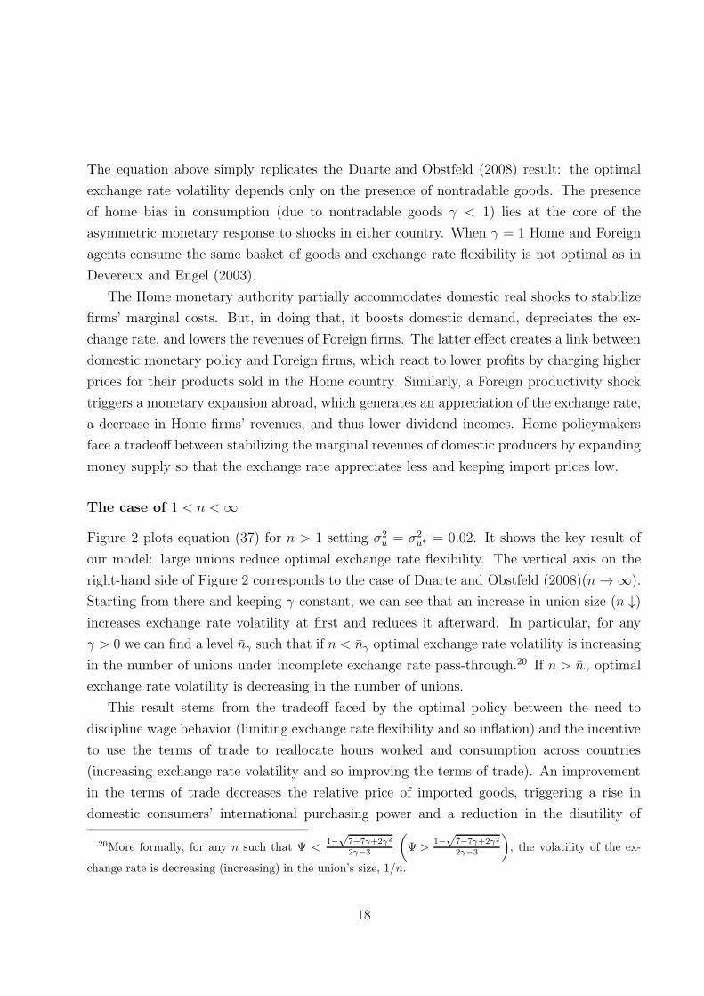
Figure 2 plots equation (37) for n > 1 setting σ2u = σ2
u∗ = 0.02. It shows the key result of
our model: large unions reduce optimal exchange rate flexibility. The vertical axis on the
right-hand side of Figure 2 corresponds to the case of Duarte and Obstfeld (2008)(n → ∞).
Starting from there and keeping γ constant, we can see that an increase in union size (n ↓)increases exchange rate volatility at first and reduces it afterward. In particular, for any
γ > 0 we can find a level nγ such that if n < nγ optimal exchange rate volatility is increasing
in the number of unions under incomplete exchange rate pass-through.20 If n > nγ optimal
exchange rate volatility is decreasing in the number of unions.
This result stems from the tradeoff faced by the optimal policy between the need to
discipline wage behavior (limiting exchange rate flexibility and so inflation) and the incentive
to use the terms of trade to reallocate hours worked and consumption across countries
(increasing exchange rate volatility and so improving the terms of trade). An improvement
in the terms of trade decreases the relative price of imported goods, triggering a rise in
domestic consumers’ international purchasing power and a reduction in the disutility of
20More formally, for any n such that Ψ <1−
√7−7γ+2γ2
2γ−3
(Ψ >
1−√
7−7γ+2γ2
2γ−3
), the volatility of the ex-
change rate is decreasing (increasing) in the union’s size, 1/n.
18

Figure 2: Exchange rate volatility vart−1(εLCPt )
labor as the burden of production is shifted abroad. Optimal monetary policy can achieve
an improvement in the terms of trade by increasing exchange rate volatility; on the other
hand, it can achieve wage discipline and lower inflation by limiting exchange rate changes.21
The importance of nontraded goods, captured by γ, determines the relevant range for op-
timal exchange rate volatility between zero and a maximum value. In Figure 2 this maximum
value is the volatility associated with the isoquant tangent to the horizontal line through
the specific value of γ.22 The number of unions in the economy, n, pins down the optimal
volatility for the economy within this range. When n > nγ, the wage markup is low and
the term-of-trade externality dominates so that a reduction in n demands more exchange
rate flexibility. Vice versa, when n < nγ the need to discipline wage behavior dominates
and a reduction in n requires limiting exchange rate volatility. The effect of non-atomistic
unions on optimal exchange rate volatility is stronger in the presence of few large unions –
this corresponds to the left-hand side of Figure 2, where the isovariance curves are steeper.
21This is in line with the empirical findings in Daniels, Nourzad, and VanHoose (2006) and Cavallari(2001).
22For a given γ, this is the optimal exchange rate volatility for n = nγ .
19
For the calibration used in Figure 2 and γ = 0.4, going from n = 2 to n = 3 sectoral unions
requires an 80 percentage point increase in exchange rate volatility.
It is worth noticing that, in contrast with Devereux and Engel (2003) and Duarte and Obstfeld
(2008), a fixed exchange rate is not necessarily optimal under LCP when Home and Foreign
agents consume the same basket of goods. Figure 2 in fact shows that optimal exchange rate
volatility is not zero for γ = 1. This stems from the fact that employment deviates from
its flexible-price counterpart (see Appendix C) when unions are non-atomistic and optimal
monetary policy faces a tradeoff between restraining exchange rate movements and allowing
some exchange rate fluctuations in order to stabilize employment.
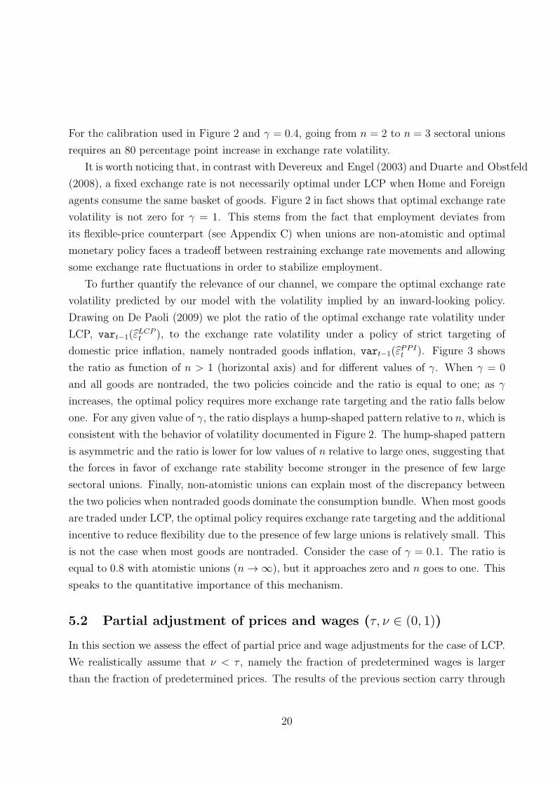
To further quantify the relevance of our channel, we compare the optimal exchange rate
volatility predicted by our model with the volatility implied by an inward-looking policy.
Drawing on De Paoli (2009) we plot the ratio of the optimal exchange rate volatility under
LCP, vart−1(εLCPt ), to the exchange rate volatility under a policy of strict targeting of
domestic price inflation, namely nontraded goods inflation, vart−1(εPPIt ). Figure 3 shows
the ratio as function of n > 1 (horizontal axis) and for different values of γ. When γ = 0
and all goods are nontraded, the two policies coincide and the ratio is equal to one; as γ
increases, the optimal policy requires more exchange rate targeting and the ratio falls below
one. For any given value of γ, the ratio displays a hump-shaped pattern relative to n, which is
consistent with the behavior of volatility documented in Figure 2. The hump-shaped pattern
is asymmetric and the ratio is lower for low values of n relative to large ones, suggesting that
the forces in favor of exchange rate stability become stronger in the presence of few large
sectoral unions. Finally, non-atomistic unions can explain most of the discrepancy between
the two policies when nontraded goods dominate the consumption bundle. When most goods
are traded under LCP, the optimal policy requires exchange rate targeting and the additional
incentive to reduce flexibility due to the presence of few large unions is relatively small. This
is not the case when most goods are nontraded. Consider the case of γ = 0.1. The ratio is
equal to 0.8 with atomistic unions (n → ∞), but it approaches zero and n goes to one. This
speaks to the quantitative importance of this mechanism.
5.2 Partial adjustment of prices and wages (τ, ν ∈ (0, 1))
In this section we assess the effect of partial price and wage adjustments for the case of LCP.
We realistically assume that ν < τ , namely the fraction of predetermined wages is larger
than the fraction of predetermined prices. The results of the previous section carry through
20

Figure 3: Ratio of exchange rate volatility under optimal policy and under strict targetingof domestic inflation, vart−1(ϵLCP
t )/vart−1(ϵPPIt )
this more general case: optimal exchange rate volatility displays a hump-shaped pattern
relative to the number of unions.
Price rigidity. Partial price adjustment implies a fraction τ of firms with constant real
marginal cost and revenue. Relative to the case of predetermined prices, unions anticipate a
smaller impact of their wage claims on the equilibrium allocation. To the extent that wages
and prices move instantaneously, productivity shocks (and exchange rate movements under
LCP) do not shift the marginal cost (revenue) and the level of employment remains constant.
As a result, wage responses are stronger. This implies that as τ goes up and more firms can
adjust their prices, the cost in terms of consumption of inflationary wage hikes dominates.
Hence, as τ goes up the optimal exchange rate volatility goes down.
Wage rigidity. As ν increases, wages are more flexible and the optimal policy has a
stronger incentive to manipulate the terms of trade. Intuitively, unions anticipate that firms
will not have an opportunity to adjust their prices in response to shocks and increase wages
in response to a positive productive shock, which in turn reduces employment and increases
21
workers’ consumption. Optimal monetary policy may want to reinforce this mechanism with
a larger depreciation if the wage markup is not too high, namely if union size is small. This
implies that, for any given γ, the hump-shaped pattern of optimal exchange rate volatility
relative to the number of unions shifts toward the left, thereby extending the range of n
where the terms-of-trade externality dominates optimal monetary policy and exchange rate
volatility is inversely related to n.
5.3 Monetary Policy Coordination
Are there gains from monetary coordination? Suppose monetary policies are chosen to
maximize a weighted average of Home and Foreign expected utility:
max!mt,!m∗
t
Et−1
[1
2Ut +
1
2U∗t
]. (40)
Cooperative and non-cooperative optimal monetary policies are equal and therefore there
are no gains from cooperation in three cases. The first case is with PCP when all wages are
flexible (ν = 1). As in Obstfeld and Rogoff (2002) and Corsetti and Pesenti (2005), optimal
monetary policies are “inward looking” with price stickiness only. The nominal exchange
rate fluctuates with relative productivity shocks, thereby moving the terms of trade and
closing the domestic output gap. The other two cases arise under LCP. One is when unions
are atomistic, wages are flexible and prices are fully predetermined (n → ∞, ν = 1, τ = 0);
the other is when wages are set by a single sectoral union (i.e. n → 1) and wages are flexi-
ble. International spillovers typically arise because non-atomistic unions affect employment
volatility by responding to exchange rate movements. In the two cases outlined above there
are no spillovers between countries and monetary policies are strategically independent of
each other.
5.4 Model-Data Comparison
Although the focus of our paper is normative, in this section we document the relationship be-
tween the optimal exchange-rate volatility under LCP predicted by our model, vart−1(ϵLCPt ),
and the actual nominal exchange-rate volatility, σ2ε .
To calculate vart−1(ϵLCPt ), we need to calibrate six parameters: nominal price rigidity τ ;
nominal wage rigidity ν; the standard deviation of Home and Foreign labor productivity σu
and σu∗ ; the share of traded goods γ; and the weight Ψ that unions attach to the response
22

Table 1: Calibration
(1) (2) (3) (4) (5) (6) (7)Country (Code) τ ν σu σε Ψ γ σu∗
Austria (AT) 0.248 0.070 0.023 0.043 0.654 0.208 0.022Czech Republic (CZ) 0.223 0.116 0.039 0.107 0.661 0.326 0.041Estonia (EE) 0.234 0.199 0.065 0.089 0.709 0.378 0.079France (FR) 0.199 0.197 0.018 0.054 0.684 0.125 0.025Greece (EL) 0.218 0.339 0.034 0.055 0.767 0.126 0.072Hungary (HU) 0.171 0.026 0.047 0.118 0.688 0.238 0.032Ireland (IE) 0.303 0.146 0.024 0.067 0.570 0.250 0.035Italy (IT) 0.218 0.042 0.027 0.080 0.686 0.130 0.026Lithuania (LT) 0.367 0.421 0.126 0.065 0.684 0.332 0.194Netherlands (NL) 0.289 0.111 0.024 0.067 0.594 0.259 0.026Portugal (PT) 0.201 0.059 0.035 0.031 0.727 0.156 0.036Slovenia (SI) 0.249 0.272 0.025 0.062 0.669 0.355 0.040Spain (ES) 0.181 0.119 0.030 0.045 0.654 0.107 0.039United States (US) 0.627 0.289 0.012 0.093 0.827 0.066 0.051
to monetary innovations. We assume that a period in the model is one year.
Nominal price and wage rigidity. We use data from theWage Dynamics Network (WDN)
survey on wage and pricing policies at the firm level. The WDN survey was carried out by 17
national central banks between the end of 2007 and the first half of 2008. It provides a unique
cross-country, harmonized dataset that simultaneously measures price and wage stickiness.
We use data for the following thirteen European countries: Austria, Czech Republic, Estonia,
France, Greece, Hungary, Ireland, Italy, Lithuania, Netherlands, Portugal, Slovenia, Spain.
All countries in the sample, except the Czech Republic and Hungary, belong to the Euro
Zone. To benchmark and compare our results, we have collected data also for the United
States. Columns 1 and 2 of Table 1 report, respectively, the frequency of price and wage
changes. For European countries τ is the fraction of firms that adjusts the price of their main
product more than once a year; ν is the fraction of firms changing the wage for their main
occupational group more than once a year. We focus on employment-adjusted-weighted data.
For the United States we build on the micro evidence for price and wage setting respectively
drawn from Weber (2015) and Barattieri, Basu, and Gottschalk (2014). See Appendix D for
additional information on calculation of τ and ν.
Standard deviation of labor productivity and the nominal exchange rate. We use
annual observations from Feenstra, Inklaar, and Timmer (2015), also known as the Penn
23

World Tables, Release 8.1. For labor productivity, we take the log of output-side PPP-
adjusted real GDP per worker and then apply the Hodrick-Prescott filter. Since the WDN
survey was conducted between 2007 and 2008, we covers a sample period 1950-2009 and
1970-2009 for Czech Republic, Estonia, Hungary, Lithuania and Slovenia. We calibrate the
standard deviation of foreign productivity (σu∗) so that labor volatility in the calibrated
model matches the standard deviation of HP residuals of log employment in the data. This
target is arbitrarily chosen to emphasize that we consider this model mostly illustrative and
not able to generate realistic predictions for the overall level of volatility in the economy.
For the nominal exchange rate, we use data from BIS on nominal effective exchange rate
indices from 1994:1 to 2009:12. We then calculate the standard deviation of the HP residuals
for domestic productivity and the nominal exchange rate. See Appendix D for further
details. The standard deviation of real GDP per worker and the standard deviation of
foreign productivity are respectively reported in column 3 and 7 of Table 1. The standard
deviation of the nominal exchange rate is reported in column 4.
Labor market concentration and openness. In our model 1/n captures the degree of
centralization in wage setting. We have no data on σ, the elasticity of substitution across
labor types, for a large set of countries. Since there is a monotonic relationship between
Ψ and n (see footnote 16), we approximate Ψ with 1 −√Haff , where Haff denotes the
mean value of the sectorial Herfindal index of union concentration – see Appendix D for data
sources. Ψ values for each country are reported in column 5 of Table 1
We measure γ as the degree of openness. Following Duarte, Restuccia, and Waddle (2007),
we construct openness as γ = exp+imp2(gdp+imp) , where exp denotes exports of goods and services
at constant national 2005 prices, imp are imports of goods and services at constant national
2005 prices, and gdp indicates GDP at constant national 2005 prices. The measure of
openness ranges between zero and one and it is reported in column 6 of Table 1.
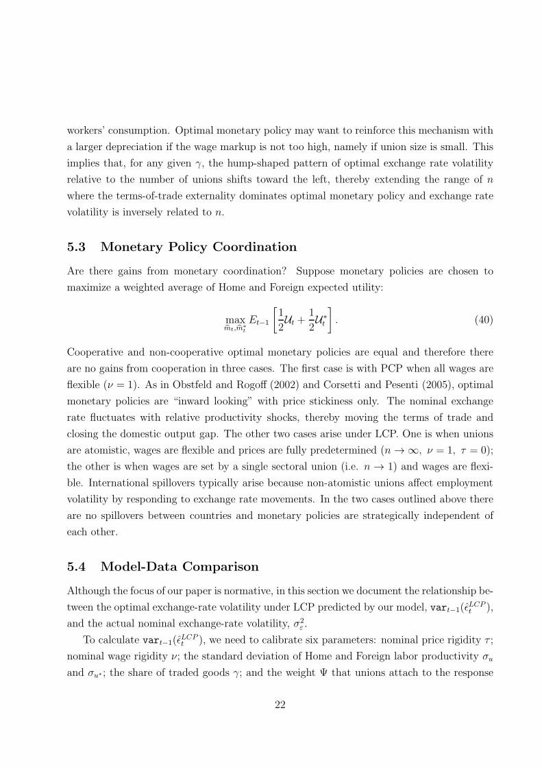
Using the parameters specified in Table 1 we calculate the optimal exchange-rate volatility
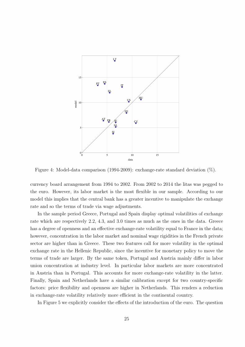
predicted by our model, (vart−1(ϵLCPt )). Figure 4 reports the the optimal exchange-rate
volatility on the vertical axis and the observed one on the horizontal axis in the sample period
1994-2009 for each country. The discrepancy between optimal and observed volatility of
exchange rate is arguably small for most countries in our sample except Lithuania, Portugal,
Spain and Greece. In particular, the optimal volatility of exchange rate for these countries
is higher than the exchange-rate volatility in the data.
Regarding Lithuania, the model predicts that the optimal volatility should be 2.8 times
as much as the volatility in the data. Lithuania pegged the litas to the US dollar under a
24
!
!
!
!
!
!
!
!
!
!
!
!
!
!
ATCZ
EE
FR
EL
HU
IE
IT
LT
NL
PT
SI
ES
US
0 5 10 150
5
10
15
data
model
Figure 4: Model-data comparison (1994-2009): exchange-rate standard deviation (%).
currency board arrangement from 1994 to 2002. From 2002 to 2014 the litas was pegged to
the euro. However, its labor market is the most flexible in our sample. According to our
model this implies that the central bank has a greater incentive to manipulate the exchange
rate and so the terms of trade via wage adjustments.
In the sample period Greece, Portugal and Spain display optimal volatilities of exchange
rate which are respectively 2.2, 4.3, and 3.0 times as much as the ones in the data. Greece
has a degree of openness and an effective exchange-rate volatility equal to France in the data;
however, concentration in the labor market and nominal wage rigidities in the French private
sector are higher than in Greece. These two features call for more volatility in the optimal
exchange rate in the Hellenic Republic, since the incentive for monetary policy to move the
terms of trade are larger. By the same token, Portugal and Austria mainly differ in labor
union concentration at industry level. In particular labor markets are more concentrated
in Austria than in Portugal. This accounts for more exchange-rate volatility in the latter.
Finally, Spain and Netherlands have a similar calibration except for two country-specific
factors: price flexibility and openness are higher in Netherlands. This renders a reduction
in exchange-rate volatility relatively more efficient in the continental country.
In Figure 5 we explicitly consider the effects of the introduction of the euro. The question
25

!
!!
!
!
!
!
!
!
!
!
!
!
!
AT
CZ EE
FR
EL
HU
IE
IT
LT
NL
PT
SI
ES
US
0 5 10 15 20 25 300
5
10
15
20
25
30
data
model
Figure 5: Model-data comparison (1994-1998): exchange-rate standard deviation (%).
arises whether optimal and effective exchange-rate dynamics differ after the introduction of
the euro in comparison with the period before the start of the European Monetary Union
(EMU). Split sample analysis for the pre-1999 period reveals a limited impact on the previous
results except for Hungary. This country in the pre-99 period was relatively a closer economy
than in the post-99 period. The degree of openness moved from 0.16 to 0.41, thereby calling
for less exchange-rate volatility.
6 Concluding remarks
We develop a tractable, stochastic model in line with the NOEM approach with nontraded
goods, incomplete exchange rate pass-through and sectoral non-atomistic unions. In this
environment we characterize optimal monetary policy and its consequences for exchange rate
volatility. Our main finding is that, under LCP, sufficient concentration in the labor market
reduces optimal exchange rate volatility even in the presence of nontraded goods. With
pricing-to-market exchange rate flexibility does not align consumer prices across borders but
rather leads to more volatile firm profits and higher prices and wages when unions are large.
By committing to reduce exchange rate fluctuations optimal monetary policy can also reduce
26

inflationary wage demands.
Our findings have policy implications. Commitment of monetary policy goes an extra
step in models with large players - large unions in our case - because these players take into
account the monetary policy response to their actions. In particular, risk leads to suboptimal
wage setting in our setting. By limiting exchange rate volatility optimal monetary policy
can reduce risk and moderate unit labor costs. We believe this is one mechanism, possibly
among others, at the heart of the desire for a stable currency in open economies. Our result
suggests that an explicit commitment to moderate exchange rate fluctuations is beneficial.
References
Acocella, N., G. Di Bartolomeo, and P. Tirelli (2007): “Monetary conservatism
and fiscal coordination in a monetary union,” Economics Letters, 94(1), 56–63.
Aidt, T. S., and Z. Tzannatos (2008): “Trade unions, collective bargaining and
macroeconomic performance: a review,” Industrial Relations Journal, 39(4), 258–295.
Barattieri, A., S. Basu, and P. Gottschalk (2014): “Some Evidence on the
Importance of Sticky Wages,” American Economic Journal: Macroeconomics, 6.
Benigno, P., and M. Woodford (2005): Optimal Stabilization Policy When Wages and
Prices Are Sticky: The Case of a Distorted Steady State.pp. 127 – 180. Washington,
D.C.: Board of Governors of the Federal Reserve System.
Bertola, G., F. D. Blau, and L. M. Kahn (2002): “Comparative Analysis of
Employment Outcomes: Lessons for the United States from International Labor Market
Evidence,” in The Roaring Nineties: Can Full Employment Be Sustained?, ed. by
A. Krueger, and R. Solow. Russell Sage and Century Foundations.
Bertola, G., and A. Ichino (1995): “Wage Inequality and Unemployment: United
States versus Europe,” in NBER Macroeconomics Annual 1995, Volume 10, NBER
Chapters, pp. 13–66. National Bureau of Economic Research, Inc.
Blanchard, O., and J. Wolfers (2000): “The Role of Shocks and Institutions in the
Rise of European Unemployment: The Aggregate Evidence,” Economic Journal,
110(462), C1–33.
27
Boeri, T., and J. van Ours (2008): The Economics of Imperfect Labor Markets.
Princeton University Press.
Booth, A. L. (1995): The Economics of the Trade Uinon. Cambridge University Press.
Bruno, M., and J. Sachs (1985): Economics of worldwide stagflation. Harvard
University Press, Cambridge, MA.
Calmfors, L., and J. Driffill (1988): “Bargaining Structure, Corporatism, and
Macroeconomic Performance,” Economic Policy, 6, 14–61.
Campa, J. M., and L. S. Goldberg (2005): “Exchange Rate Pass-Through into Import
Prices,” The Review of Economics and Statistics, 87(4), 679–690.
Campolmi, A., and E. Faia (2009): “Optimal Choice of Exchange Rate Regimes with
Labour Market Frictions,” mimeo.
Cavallari, L. (2001): “Inflation and Openness with Non-Atomistic Wage Setters,”
Scottish Journal of Political Economy, 48(2), 210–25.
Clarida, R., J. Gali, and M. Gertler (2001): “Optimal Monetary Policy in Open
versus Closed Economies: An Integrated Approach,” American Economic Review, 91(2),
248–252.
Coricelli, F., A. Cukierman, and A. Dalmazzo (2004): “Economic Performance
and Stabilisation Policy in a Monetary Union with Imperfect Labor and Goods’
Markets,” in European Monetary Integration, ed. by H. W. Sinn, M. Widgren, and
M. Kothenburger. MIT Press, Cambridge, MA.
Corsetti, G. (2006): “Openness and the case for flexible exchange rates,” Research in
Economics, 60(1), 1–21.
Corsetti, G., L. Dedola, and S. Leduc (2010): “Optimal Monetary Policy in Open
Economies,” in Handbook of Monetary Economics, ed. by B. M. Friedman, and
M. Woodford, vol. 3 of Handbook of Monetary Economics, chap. 16, pp. 861–933.
Elsevier.
Corsetti, G., and P. Pesenti (2005): “International dimensions of optimal monetary
policy,” Journal of Monetary Economics, 52(2), 281–305.
28

Cubitt, R. P. (1992): “Monetary Policy Games and Private Sector Precommitment,”
Oxford Economic Papers, 44(3), 513–30.
Cuciniello, V. (2011): “The Welfare Effect of Foreign Monetary Conservatism with
Nonatomistic Wage Setters,” Journal of Money, Credit and Banking, 43(8), 1719–1734.
(2013): “Large labour unions and terms-of-trade externality,” Economics Letters,
120(1), 135–138.
Cukierman, A., and F. Lippi (2001): “Labour Markets and Monetary Union: A
Strategic Analysis,” Economic Journal, 111(473), 541–65.
Daniels, J. P., F. Nourzad, and D. D. VanHoose (2006): “Openness, centralized
wage bargaining, and inflation,” European Journal of Political Economy, 22, 969–988.
De Paoli, B. (2009): “Monetary policy and welfare in a small open economy,” Journal of
International Economics, 77(1), 11–22.
Devereux, M. B., and C. Engel (2003): “Monetary Policy in the Open Economy
Revisited: Price Setting and Exchange-Rate Flexibility,” Review of Economic Studies,
70(4), 765–783.
Du Caju, P., E. Gautier, D. Momferatou, and M. Ward-Warmedinger (2009):
“Institutional features of wage bargaining in 23 European countries, the US and Japan,”
Ekonomia, 12(974), 57–108.
Duarte, M., and M. Obstfeld (2008): “Monetary Policy in the Open Economy
Revisited: The Case for Exchange-Rate Flexibility Restored,” Journal of International
Money and Finance, 27, 949–957.
Duarte, M., D. Restuccia, and A. L. Waddle (2007): “Exchange rates and business
cycles across countries,” Economic Quarterly, (Win), 57–76.
Elsby, M. W., B. Hobijn, and A. Sahin (2011): “Unemployment Dynamics in the
OECD,” Tinbergen Institute Discussion Papers 11-159/3, Tinbergen Institute.
Engel, C. (2011): “Currency Misalignments and Optimal Monetary Policy: A
Reexamination,” American Economic Review, 101(6), 2796–2822.
29
Engel, C., and J. H. Rogers (1996): “How Wide Is the Border?,” American Economic
Review, 86(5), 1112–25.
Feenstra, R. C., R. Inklaar, and M. Timmer (2015): “The Next Generation of the
Penn World Table,” American Economic Review, forthcoming.
Friedman, M. (1953): “The Case for Flexible Exchange Rates,” in Essays in Positive
Economics, pp. 157–203. The University of Chicago Press.
Goldberg, P. K., and M. M. Knetter (1997): “Goods Prices and Exchange Rates:
What Have We Learned?,” Journal of Economic Literature, 35(3), 1243–1272.
Gruner, H. P., and C. Hefeker (1999): “How Will EMU Affect Inflation and
Unemployment in Europe?,” Scandinavian Journal of Economics, 101(1), 33–47.
Holden, S. (2003): “Wage setting under different monetary regimes,” Economica, 70(2),
251–265.
Ilzetzki, E., C. M. Reinhart, and K. S. Rogoff (2008): “Exchange Rate
Arrangements Entering the 21st Century: Which Anchor Will Hold?,” Mimeo.
Jensen, H. (1993): “International monetary policy cooperation in economies with
centralized wage setting,” Open Economies Review, 4(3), 269–285.
Nickell, S., L. Nunziata, and W. Ochel (2005): “Unemployment in the OECD Since
the 1960s. What Do We Know?,” Economic Journal, 115(500), 1–27.
Obstfeld, M., and K. Rogoff (2002): “Global Implications Of Self-Oriented National
Monetary Rules,” Quarterly Journal of Economics, 117(2), 503–535.
OECD (2009): Employment Oulook. Paris: OECD.
Soskice, D., and T. Iversen (1998): “Multiple Wage-Bargaining Systems in the Single
European Currency Area,” Oxford Review of Economic Policy, 14(3), 110–24.
Tarantelli, E. (1986): Economia politica del lavoro. UTET, Torino.
Vartiainen, J. (2002): “Relative Prices in Monetary Union and Floating,” Scandinavian
Journal of Economics, 104(1), 277–287.
30

Veracierto, M. (2008): “Firing Costs And Business Cycle Fluctuations,” International
Economic Review, 49(1), 1–39.
Weber, M. (2015): “Nominal Rigidities and Asset Pricing,” mimeo.
Appendix
A Impact of union’s wage on aggregate wage
From the wage index (13), we obtain
∂Wt
∂Wt(x)=
∂
∂Wt(x)
[∫ 1
0
Wt(z)1−σdz
] 11−σ
=∂
∂Wt(x)
[∫
z∈x
Wt(z)1−σdz +
∫
z /∈x
Wt(z)1−σdz
] 11−σ
=1
n
[Wt(x)
Wt
]−σ
=1
n(A.1)
where the last equality holds in a symmetric equilibrium, i.e. when W (x) = W .
B Derivation of the optimal wage setting
From eq. (4) and (5) the exchange rate can be expressed as
Et =Mt
M∗t
. (B.1)
For a given level of foreign monetary policy stance, an expansionary monetary policy shock
(higher Mt and higher nominal expenditure PtCt in equilibrium) is associated with a depre-
ciation of the exchange rate.
From the aggregate goods market clearing conditions we obtain the following aggregate
labor demands:
LHt =γ
2At
(PtCt
PHt+
P ∗t C
∗t
P ∗Ht
)=
γ
2At
Mt
PHt
(1 +
PHt
EtP ∗Ht
)(B.2)
31

LNt =1− γ
At
PtCt
PNt=
1− γ
At
Mt
PNt, (B.3)
where we used (B.1).
Without nominal rigidities, the law of one price holds (EtP ∗Ht = PHt) and employment is
given by
LflexHt =
γ
Mp
Mt
WHtLflexNt =
1− γ
Mp
Mt
WNt. (B.4)
The elasticity of aggregate labor demand to wage is
−∂ logLflex
jt
∂ logWjt= 1, j ∈ {H,N}. (B.5)
The elasticity of aggregate labor demand for labor type z (14) to wage with flexible prices is
−∂ logLflex
jt (x)
∂ logWjt(x)= σ
(1−
1
n
)+
1
nj ∈ {H,N}, (B.6)
where we used (A.1) taking monetary stance as given.
Now, each union maximizes
Vjt(x) = n
∫
z∈x
[1
MtWjt(x)Ljt(z)− kLjt(z)
]dz j ∈ {H,N}, (B.7)
with respect to Wjt(x) subject to the labor demand (14), the budget constraint (3) and the
optimal price setting (15).
The first-order condition for unions operating in the non-traded goods sector is
0 = (1− σ)LNt(i)
Mt+
σ
n
WNt(i)
WNt
LNt(i)
Mt−
τ
n
WNt(i)LNt(i)
MtWNt+
τ − 1
nAt
WNt(i)LNt(i)
MtEt−1WNt
At
+
+σkLNt(i)
WNt(i)+
τ
nkLNt(i)
WNt−
τ − 1
nAtk
LNt(i)
Et−1WNt
At
− σkLNt(i)
nWNt. (B.8)
In a symmetric equilibrium, WNt(i) = WNt, the above expression boils down to
0 =LNt
Mt
[
1− σ +σ
n−
τ
n+
τ − 1
nAt
WNt
Et−1WNt
At
]
+
+kLNt
Mt
[
σMt
WNt+
τ
n
Mt
WNt−
τ − 1
nAt
Mt
Et−1WNt
At
− σMt
nWNt
]
. (B.9)
32

Thus, the steady state level of the first-order condition is given by
WN
M= k
[1 +
n
(n− 1)(σ − 1)
]= kMw. (B.10)
Log-linearizing (B.9) around the symmetric steady state (B.10) yields eq. (31) in the text.
Under PCP, the first-order condition for unions operating in the tradables is
0 = 2WHtLHt
Mt
[1− σ
WHt
(1−
1
n
)+
1− τ
nWHt+
τ − 1
nAt
1
Et−1WHt
At
]
+
+2kLHt
[σ
WHt
(1−
1
n
)+
τ
nWHt−
τ − 1
nAt
1
Et−1WHt
At
]
. (B.11)
Under LCP, the first-order condition for unions operating in the tradables is
0 =WHtLHt
Mt
⎡
⎣21− σ
WHt
(1−
1
n
)+ 2
1− τ
nWHt+
τ − 1
nAt
1
Et−1WHt
At
+τ − 1
nAt
E−1t
Et−1WHtE
−1t
At
⎤
⎦+
+kLHt
⎡
⎣2σ
WHt
(1−
1
n
)+ 2
τ
nWHt−
τ − 1
nAt
1
Et−1WHt
At
−τ − 1
nAt
E−1t
Et−1WHtE
−1t
At
⎤
⎦ . (B.12)
Notice that the steady state of (B.11) and (B.12) is equal to (B.10). Log-linearizing (B.11)
and (B.12) around that steady state yields (32) in the text.
C Derivation of expected utility
In order to derive the expected utility function that the monetary authority seeks to maxi-
mize, we start from expected consumption:
Et−1 logCflex
t
Cjt
= Et−1 log
(Cflex
t
Cjt
)1−τ
= (1− τ)Et−1
{log
Mt
P flext
− logMt
P jt
}=
= (1− τ)Et−1
{pjt − pflext
}j ∈ {PCP, LCP}, (C.1)
33

where
Et−1 logPLCPt
P flext
= Et−1 log
[Et−1
WHt
At
] γ2[Et−1
EtW ∗
Ft
A∗
t
] γ2[Et−1
WNt
At
]1−γ
[WHt
At
] γ2[EtW ∗
Ft
A∗
t
] γ2[WNt
At
]1−γ
=γ
2
[σ2wH
2+
σ2u
2− σwHu − σw∗
F u∗ + σw∗
F ε − σεu∗ +σ2w∗
F
2+
σ2u∗
2+
σ2ε
2
]
+(1− γ)
[σ2wN
2+
σ2u
2− σwNu
]
=γ
2
[Et−1(wHt − at)2
2+
Et−1(w∗Ft − a∗t + εt)2
2
]+ (1− γ)
Et−1(wNt − at)2
2
(C.2)
and
Et−1 logP PCPt
P flext
= Et−1 log
[Et−1
WHt
At
] γ2[EtEt−1
W ∗
Ft
A∗
t
] γ2[Et−1
WNt
At
]1−γ
[WHt
At
] γ2[EtW ∗
Ft
A∗
t
] γ2[WNt
At
]1−γ
=γ
2
[σ2wH
2+
σ2u
2− σwHu − σw∗
F u∗ +σ2w∗
F
2+
σ2u∗
2
]
+ (1− γ)
[σ2wN
2+
σ2u
2− σwNu
]
=γ
2
[Et−1(wHt − at)2
2+
Et−1(w∗Ft − a∗t )
2
2
]+ (1− γ)
Et−1(wNt − at)2
2. (C.3)
We now turn to expected employment. In order to be able to arrive at a closed-form so-
lution without having to resort to numerical simulation, we will approximate the exponential
terms in the welfare functions by linear expressions. For example, exp(xt) is approximated
34

by 1 + xt. Using (B.2) and (B.4) we obtain
Et−1
{LflexHt − LLCP
Ht
}=
γ
MpEt−1
{Mt
WHt−
Mt
2At
(WHt
At
)−τ[(
Et−1WHt
At
)τ−1
+E τ−1t
(Et−1
WHt
AtEt
)τ−1]}
=γ
kMp(1− τ)
{σ2wH
+σεm − σεwH
2+ σmu − σmwH
− σwHu
+τ
2
[σ2ε
2+ σ2
u + σ2wH
+ σεu − σεwH− 2σwHu
]}
=γ
kMp(1− τ)Et−1
{(wHt − mt)(wHt −
εt2− at)
+τ
2
[
(wHt −εt2− at)
2 +
(εt2
)2]}
,
(C.4)
Et−1
{LflexHt − LPCP
Ht
}=
γ
MpEt−1
{Mt
WHt−
Mt
At
[(Et−1
WHt
At
)τ−1(WHt
At
)−τ]}
=γ
kMp(1− τ)
{σ2wH
+ σmu − σmwH− σwHu +
τ
2
[σ2u + σ2
wH− 2σwHu
]}
=γ
kMp(1− τ)Et−1
{(wHt − mt)(wHt − at) +
τ
2(wHt − at)
2}. (C.5)
Similarly, from (B.3) and (B.4) we can write the following expression:
Et−1
{LflexNt − LNt
}=
1− γ
MpEt−1
{Mt
WNt−
Mt
At
[(Et−1
WNt
At
)τ−1(WNt
At
)−τ]}
=1− γ
kMp(1− τ)
{σ2wN
+ σmu − σmwN− σwNu +
τ
2
[σ2u + σ2
wN− 2σwNu
]}
=1− γ
kMp(1− τ)Et−1
{(wNt − mt)(wNt − at) +
τ
2(wNt − at)
2}. (C.6)
Thus, the expected utility under LCP and PCP is given respectively by
Et−1
{Uflext − ULCP
t
}= (1− τ)(C.2)− k(C.4)− k(C.6) (C.7)
35
and
Et−1
{Uflext − UPCP
t
}= (1− τ)(C.3)− k(C.5)− k(C.6). (C.8)
Expressions (35) in the text are derived by maximizing the above expected utilities with
respect to mt, subject to the optimal wage decisions (31) and (32) and setting τ = 0 and
ν = 1.
D Data
Price and Wage StickinessFor European countries we use Wage Dynamics Network Data from the European Central
Bank. Data on price changes are taken from Question 31: “Under normal circumstances, how
often is the price of the firm’s main product typically changed?”. τ in Table 1 corresponds
to the frequency of firms that change their price more than once a year. Data on wage
changes are collected from Question 9: “How frequently is the base wage of an employee
belonging to the main occupational group in your firm typically changed in your firm?”
We set ν in Table 1 equal to the highest frequency of firm-level wage change among the
type more than once a year whose determinants are unrelated to tenure and/or inflation or
due to tenure or due to inflation. We adopt employment-adjusted weights, where the weight
attached to each firm in the sample refers to how many employees that observation represents
in the population. For the United States we build on the micro evidence for price and
wage setting, respectively drawn from Weber (2015) and Barattieri, Basu, and Gottschalk
(2014). Barattieri, Basu, and Gottschalk (2014) estimate an average quarterly probability
of a nominal wage change between 21.1 and 26.6 percent. As for Wage Dynamics Network
data, we choose the highest frequency. Weber (2015) estimates that prices are expected to
remain unchanged for 2.17 quarters. From expected lifetime of prices we can infer the Calvo
parameter, namely price remains unchanged with probability equals to 0.54 each quarter.
Now, in order to calculate the probability of changing prices/wages more than once a year, we
apply the following formula∑4
t=2
(4t
)xt (1− x)4−t, where x is equal to 46.1 and 26.6 percent
for getting respectively τ and ν in Table 1.
Labor ProductivityWe use data from the Penn World Tables, Release 8.1. The standard deviation of labor
productivity σu is calculated as follows: a) we calculate PPP-adjusted real GDP per worker
36

as rgdpo/emp; b) we take log and then apply the Hodrick-Prescott filter with smoothing
parameter equal to 100; c) we calculate the standard deviation of HP residuals. The standard
deviation σu∗ is pinned down so that volatility of employment in the calibrated model matches
volatility of employment calculated as the standard deviation of HP residuals of the log of
emp.
Nominal Exchange RateWe use monthly BIS nominal, broad effective exchange rate indices for the 1994:1-2009:12
period. The standard deviation of nominal effective exchange rate is calculated as follows:
a) we take log and then apply the Hodrick-Prescott filter with smoothing parameter equal
to 14400; b) we calculate the standard deviation of HP residuals; c) we multiply monthly
standard deviation of HP residuals by√12 so as to obtain annualized standard deviations.
Labor Market ConcentrationWe use data from the ICTWSS Database on Institutional Characteristics of Trade Unions,
Wage Setting, State Intervention and Social Pacts. We set Ψ equal to 1 −√Haff , the
Herfindahl index at sectoral level of union membership concentration. The variable Haff
takes values between 0 and 1. We take the average value of Haff over the entire sample
period for each country.
OpennessData are collected from the Penn World Tables, Release 8.1. Openness is measured asexp+imp
2(gdp+imp) , where exp denotes exports of goods and services, imp are imports of goods and
services, and gdp indicates GDP. All variables are measured at constant national 2005 prices.
We take the average value over the entire sample period for each country. This measure of
openness ranges between zero and one: zero when both export and imports are zero; one as
output and domestic spending approach zero and the value of exports equals the value of
imports.
37
Recommended