Optimal Dynamic Production from a Large Oil Field in Saudi Arabia1
Weiyu Gao
Economic Development Research Center Shanghai, China [email protected]
Peter R. Hartley
Department of Economics, Rice University Houston, Texas [email protected]
Robin C. Sickles
Department of Economics, Rice University Houston, Texas [email protected]
Abstract
We model the economically optimal dynamic oil production decisions for a stylized oilfield
resembling the largest developed field in Saudi Arabia, Ghawar, paying particular attention to the
engineering aspects of oil production. Specifically, we begin with a fluid dynamics model
composed of differential equations describing the dynamics of fluid flow as a function of fluid
pressure, formation characteristics, water injection, new wells, and how these parameters change
as oil extraction occurs. We then link this physical description of the field to an intertemporal
optimizing economic model. The cost and revenue functions are based on data from a number of
sources. We use tensor splines to approximate the value function. The optimal solution depends on
exogenous variables, such as the discount rate or the timing of breakthroughs in the cost of
alternative energy sources, which are uncertain. We examine solutions under a number of
scenarios to account for these uncertainties.
JEL Classification System Number: C30, C61, Q32, Q41
Keywords: Optimal oil production; Dynamic programming; Value function
approximation
1 Funding for this study was provided by a grant from the Center for International Political Economy (CIPE) to the James A. Baker III Institute for Public Policy at Rice University. The authors would like to thank Dr. Stephen Rester of Haliburton Industries and international industry expert and private consultant Richard Martin of Houston for their vital contributions in data analysis and in providing modeling expertise that allowed us to simulate the temporal patterns of reservoir production used in our analysis. The usual caveat applies.

1
1. Introduction
Following the Arab oil embargo of 1973–74, which produced a four-fold increase
in world oil prices, understanding oil market dynamics, and especially OPEC oil
production decisions, has been a major concern for economists. Saudi Arabia, the
largest supplier in OPEC, then as now produces about 30% of total OPEC output
and about 12% of the total world output. It also has roughly 25% of the world’s
proven conventional oil reserves and a maximum sustainable production capacity
of 10.5–11 million barrels per day.2 The overwhelming influence of Saudi oil
policy on past world oil prices is widely acknowledged.
The highest levels of the Saudi Arabian government, acting through the Supreme
Council for Petroleum and Mineral Affairs, take ultimate responsibility for oil
pricing and production decisions. Revenues from oil sales, and activities such as
petrochemicals and oil refining, account for about 50% of Saudi government
expenditures (Azzam, 1993). One therefore would expect to find that the revenue,
or more particularly profits, of Saudi Aramco should be of major concern. For
example, Soligo and Jaffe (2000) point out that Saudi Arabia has been practicing
price discrimination against customers in the Far East in favor of customers in
U.S. and Europe, which is consistent with a profit maximization motive.
Economic motivations apart from profit maximization also have been proposed.
These include diversifying away from oil revenue in the long term and meeting
short-term fluctuations in government expenditure. For example, Teece (1982)
proposes that OPEC countries base production decisions on target revenues, while
Ramcharran (2002) presents evidence consistent with this hypothesis. An
implication would be that price rises should substantially reduce OPEC supply.
Non-economic factors may also influence oil policy. For example, Askari (1991)
suggests that political goals, such as Saudi’s role in the world, Arab solidarity, and
regional politics, also have motivated Saudi Arabian oil policy.
We focus on finding the dynamically optimal (profit maximizing) oil production
rate. Our analysis provides a measure of the extent to which long-run value
maximization is being followed. It also allows us to assess the potential for
2 These Saudi Arabian oil statistics were obtained from the United States Energy Information Administration web site.

2
forgone profits in the event that oil production decisions are based on criteria
other than the maximization of the expected present value of profits.3
A number of studies have addressed the oil production policies of OPEC, and
Saudi Arabia in particular, in a dynamic optimization setting. Dahl and Yücel
(1991), among others, find empirical support for the role of dynamic behavior in
producer supply decisions. Quandt (1982) qualitatively discusses Saudi Arabia’s
oil policy and its possible motivations based on two criteria: optimization of the
long-term value of oil reserves and the attainment of political goals. Khadduri
(1996) discusses the oil policies of Middle East countries in the context of current
developments in that region. Powell (1990) gives an excellent review of two
major strands of economic research on OPEC oil production. The first approach
attempts to simulate the behavior of the decision-maker. The second is the
intertemporal optimization approach, traditionally attributed to Hotelling (1931).
Recent research on oil production using dynamic value optimization has been
pursued by, among others, Wirl (1990), Suranovic (1993), Benkherouf (1994),
Lohrenz and Bailey (1995), and Fousekis and Stefanou (1996).
The novel element in our approach is that it is based on an engineering model of
oil extraction, which is an inherently dynamic process. We solve for the combined
long run investment and short run production path that maximizes discounted
profits by integrating economic factors, like demand and drilling and maintenance
costs, with petroleum engineering considerations affecting oil recovery.
Specifically, we begin our analysis with an engineering model (WorkBench Black
Oil Simulator, 1995), which recursively solves a system of homogeneous
difference equations that describe the fluid dynamics within and among a set of
three-dimensional grids that partition the oil field and whose joint behavior
describes the production dynamics of the field. Using the Black Oil simulation
results, we estimate a short-term dynamic production function linking water
injection rates, cumulative field production, and the number of oil wells to the
short-run production capacity. This dynamic production function is employed as
an inequality constraint qualifying the intertemporal profit maximization problem.
3A complete model of the optimal oil policy of a country like Saudi Arabia requires a thorough understanding of the country’s economic and political circumstances. While acknowledging the complexity, we believe there is value in focusing on profitability. In particular, even when Saudi Arabia has other goals, it is worth knowing the cost in terms of foregone profits.

3
Our approach contrasts with the traditional economics of production literature
where the production function is specifed based either on a generic property of
scale or substitution (e.g., the constant elasticity of substitution production
function) or on approximating forms (such as Cobb-Douglas, transcendental
logarithmic or Leontief). It is instead related to the work of Griffin (1977, 1978)
who constructed approximations to static technologies utilizing pseudo-data.
However, it differs from Griffin in that the production technology we consider is
fundamentally dynamic. The traditional economics of production literature also is
most often cast in a static setting with the dynamics of production subsumed in the
effects of current production on future capacity.
Our approach also differs from the extensive engineering literature based on
dynamic fluid flow models. In this literature (see Feraille et. al., 2003, for
example), the objective is usually taken to be maximization of total production
from the reservoir. We instead recognize that discounting implies future
production is valued less than production today, while for a large producer such as
Saudi Arabia additional production in any period will depress market prices.
We apply the model to a homogeneous light oil field whose properties mimic
those of Saudi Arabia’s largest field, Ghawar. While this field accounts for about
60%–70% of Saudi oil reserves, we effectively assume that all Saudi oil is
produced from a field whose properties mimic those of Ghawar. Since the
reservoir environments of Saudi oil fields differ, this simplification undoubtedly
affects the accuracy of the model predictions. Our methodology could handle
more heterogeneity. It simply would take more information and computing
resources than we had available. A complete analysis would require multiple
reservoir descriptions. There is also a lack of individual well production history
for many fields. Finally, the time and manpower needed, and computing resources
required, for a national model would be large even if the data were available.
2. Dynamic Modeling of Oil Production Decisions
Several issues are especially relevant to Saudi Arabia’s oil production decisions.
First, Saudi Arabia is a large producer in the world oil market and especially large
in terms of the reserves available for future production. We model Saudi Arabia as
a firm with monopoly power facing downward-sloping world oil demand net of
other supply. Second, oil production costs include exploration and development
4
costs in addition to the costs of producing output from existing wells. The third
issue that needs to be addressed, namely the dynamic nature of oil production, is
the main novelty of our paper. The optimal scheduling of production needs to take
effects on future reservoir productivity into account. Specifically, we assume that
current oil production affects reservoir conditions and hence future production
costs and ultimately the total resources that will be extracted from the reservoir.
A dynamic programming framework is essential to answering such questions as
the sensitivity of current output to changes in the presumed date of arrival or price
of a backstop energy technology. In turn, this is a critical issue in the current
world oil market. How much alternative supply will current oil prices engender?
The short-run investment responses may depend critically on expectations about
the future availability of alternative energy sources.
Our characterization of the dynamic programming problem differs from the
simple Hotelling model of resource extraction where a fixed level of resource is
gradually extracted over time until no resource remains. In practice, oil wells
typically are abandoned well before the reservoirs are depleted. Depletion raises
the costs of extraction until continued recovery becomes unprofitable.
In principle, one could imagine the price of oil rising continuously so that
increasingly costly secondary recovery techniques become profitable. Our model
is instead based on what we view as a far more likely scenario whereby, beyond
some period, the energy market is dominated by a backstop technology that
controls the demand for oil.4 Other recent papers examining optimal OPEC policy,
such as Berg et al. (1997), have taken some unspecified carbon-free backstop
technology, available in copious supply at a fixed price, as determining the
terminal value of oil production beyond some finite time horizon. Under those
circumstances, a well with remaining oil can be abandoned if the costs of
producing from it become too high.
Formally, we take cumulative production from the oil field as the state variable in
the dynamic optimization problem rather than the more usual level of reserves
remaining. Furthermore, we exploit the fact that the future price-taking world will
result in a stationary “tail problem” with a time invariant value function. By
4 The alternative technologies could include solar energy, nuclear fusion, the so-called “hydrogen economy”, or even the exploitation of unconventional sources of oil or the more widespread use of liquefied natural gas through expansion of the natural gas industry (Jensen, 2003).

5
contrast, the optimization problem in earlier periods will not be stationary because
we assume that the demand function for Saudi oil (total demand net of supply
from the competitive fringe) varies over time. The time-varying value functions in
the initial periods are solved using backwards recursion.
We model the optimal production policy for our hypothetical light oil field using
the following Bellman equation5
vtN
t,CP
t( ) = MaxXt ,dNt {r Xt( ) ! c X
t,dN
t,W
t,N
t( ) + "vt+1
Nt+1,CP
t+1( )} (2.1)
subject to
Nt+1 = (1 – δ)Nt + dNt and dNt ≥ 0 CPt+1 = CPt + 365Xt
Wt= w X
t,N
t,dN
t( )
0 ! Xt ! f Nt ,dNt ,Wt ,CPt( ) where X, dN, W, N, and CP stand correspondingly for oil production rate (in
millions of barrels per day, mmbd), the number of new oil wells drilled during the
period, water injected (in mmbd) to maintain the reservoir liquid pressure, the
number of producing wells at the beginning of the period, and the cumulative
production of the field. X and dN are policy variables and N and CP are state
variables. β is the discount factor, while δ reflects the proportion of producing
wells watering out during each period. The revenue function, r(X) = p(X)X, where
p is the inverse demand equation relating the equilibrium world oil market price to
Saudi supply. Increasing output requires additional water injection as specified in
the function w. The function f represents the short-term field capacity that
constitutes an upper bound for oil production during a certain period. The value
function v represents the discounted present value of profits given N and CP and
assuming that the policy variables are chosen optimally from period t forward.
5Under certain general and nonrestrictive conditions (2.1) can be shown to be equivalent to a sequence problem (SP). For these conditions, see Theorem 4.2 and 4.3 in Stokey, Lucas, and Prescott (1989). Allowing for field heterogeneity would increase the number of state variables and the dimension of the space over which v is defined. It is also easy, in principle, to extend the dynamic optimization model to allow for uncertainty. The period t+1 value function on the right side of (2.1) is replaced by its expected value conditional on information known at t. Random variables with a continuous distribution are replaced by discrete approximations and intertemporal correlation is expressed as a finite state Markov process. The current value of a random variable becomes a new state variable.
6
The time discount factor and Saudi expectations about the assumed availability of
the backstop are subjective factors about which we have very little information.
While some other critical information also is difficult to obtain, the subjective
factors are inherently uncertain. In addition, Powell (1990) argues that the
solutions to intertemporal optimization models for OPEC countries will be
strongly influenced by the future cost of oil substitutes in the terminal stationary
environment and the discount rate of the decision-makers. We have thus focused
on varying these assumed subjective factors in our scenario analysis.
We simulate the optimal production paths based on four scenarios. In all cases, the
model is non-stationary before the substitute backstop technologies are available.
In the first two scenarios, the demand curve becomes stationary at some date. The
difference between these two cases arises from different discount rates. Our
choices of discount rates (10% and 30%) are consistent with the results of
Adelman (1993a) who discusses oil-producing countries’ discount factors.
According to his research, 10% is a standard (real) discount rate for oil firms in
countries like the United States. On the other hand, for some OPEC countries like
Saudi Arabia there is substantial risk associated with exploiting oil resources
because the government relies so heavily on oil income. In effect, since oil
reserves are a risky undiversified asset, the implicit rent from leaving oil in the
ground has to yield a substantial risk premium. Hence, the discount rate may
exceed 20% or even three times the standard rate.
In the other two scenarios, future cost reductions in an oil substitute (we assume it
is solar energy) reduce the demand for oil in the terminal stationary state. These
two cases differ only in the timing of a breakthrough in producing solar energy on
a massive scale. The solar energy literature contains different predictions for the
likely cost reduction of solar energy.
Nemet (2006) notes that simple learning curve models fit to world surveys of
photovoltaic (PV) panel prices suggest that PV power could become competitive
with conventional alternatives any time between 2039 and 2067. Nemet also
argues, however, that simple learning curve models are unlikely to yield accurate
predictions since the factors with the largest effect on PV cost, namely plant size,
improvements in conversion efficiency and the cost of silicon, do not appear to be
strongly affected by learning by doing. On the other hand, plant size is strongly
affected by the size of the market. Nemet suggests that an industry growth rate of

7
11% for 45 years may not make PV competitive. Maycock (2005), however,
presents data showing that PV production worldwide grew about 43% per annum
over the five years to 2004.
The National Renewable Energy Laboratory (2007) notes that the U.S.
Department of Energy Solar Energy Technologies Program aims to reduce the
average installed cost of all grid-tied PV systems to levels competitive with
conventional alternatives by 2015. As part of that program, in March 2007 the
Department provided grants to expand annual U.S. manufacturing capacity of
solar PV from 240 MW in 2005 to 2,850 MW by 2010.
Spain recently commissioned a 20MW solar thermal plant and has started
construction on a 20MW solar PV plant. The Spanish government has announced
a target of 400 MW of grid-connected solar generating capacity by 2010. In
October 2006, an Australian firm announced a project to build a 154 MW grid-
connected PV solar plant, while in June 2007 a California firm announced a
project to build an 80 MW grid-connected PV solar plant.
In light of these developments, we adopt relatively conservative expectations in
our simulations. In one scenario, the cost of photovoltaic electricity starts to fall
below that of electricity from fossil fuel in 2036, and in the other it starts in 2026.
A ten-year transition period is assumed in both cases during which much of the
demand for Saudi Arabian oil gradually switches to solar energy.6
3. Data and Estimations
This section outlines how we obtain functional representations for the required
revenue and cost functions and the production process.
3.1 The Dynamic Production Function
Salehi-Isfahani (1995) provides a review of models of the oil market that updates
his earlier joint work in Cremér and Salehi-Isfahani (1991). In his review, Salehi-
Isfahani notes, “…Depending on the type of geological structure, oil may be lost
due to pressure and seepage. Unfortunately, the economic literature has so far not
6 Another issue that could be investigated in more detail is that different components of the energy market could abandon fossil fuel at different times. Fuel Cells or other technologies such as the use of ethanol as a fuel could displace oil from transportation applications before solar energy and electric vehicles become more competitive.

8
incorporated much technical knowledge about the operation of the fields. Mining
engineers often predict a production path from a given field as an inverted U, with
a unique peak. Economists on the other hand emphasize the role of prices in
extraction. Adelman (1993b) correctly criticizes the exhaustible resource models
for their lack of realism in the description of reserves.” Below we attempt to
address these concerns by formally modeling oil field fluid dynamics.
We use the Workbench Black Oil Simulator to model the dynamic production
characteristics of an oil field with properties typical of the giant Saudi Ghawar
field. Detail on geological characteristics and the black oil simulation exercise can
be found in the Appendix. In summary, the laws of physics, expressed as partial
differential equations, control how fluids are distributed in oil reservoirs that are
undisturbed for geologic time and how those fluids move in a reservoir once they
are disturbed by production. The fluids in place at the time of discovery become
the set of initial conditions for the partial differential equations. Mathematical
representations of wells then are added to the description and the partial
differential equations are stepped through time to predict the movement of the
fluids through the reservoir.
Wells can be used to produce fluid from the reservoir or to inject fluid into the
reservoir. Technology can control only what happens at the wells as fluid is
injected and a producing well extracts some of those fluids in its immediate
vicinity. Nature controls everything in the reservoir between the wells. The Black
Oil Simulator predicts how the fluids move in the reservoir based on the reservoir
properties and how hard the wells are produced.
We accumulated the temporal production, water injection, and well drilling
schedules from the simulations of the Workbench Black Oil software. The model
simulation algorithm varies X and finds the amount of W and N required to meet
the production levels. This allows us to characterize the input requirement set
corresponding to different (dynamic) levels of X. We then summarize
parametrically the constructed technology set using regression functions.
Regression is used here as a purely descriptive device. Using the simulation
results, we then describe two important relationships that comprise our dynamic
production function (at the full capacity) for the oil field – a water injection
function and a short-term capacity function.
9
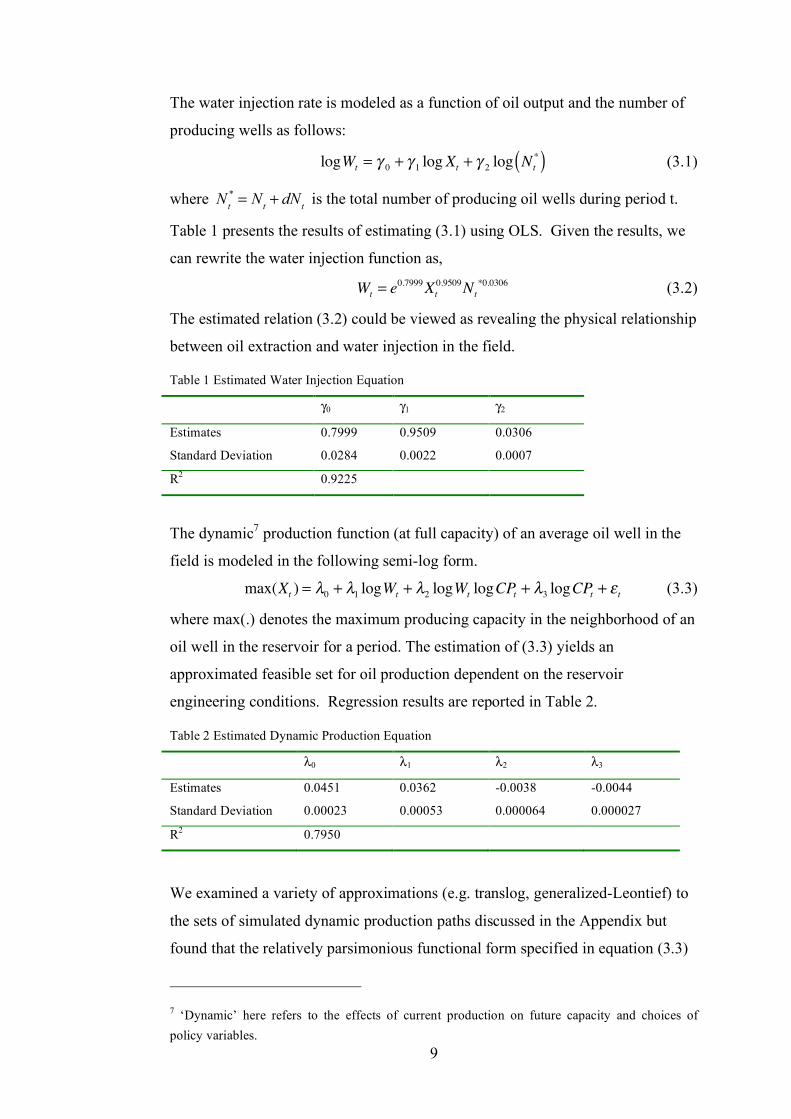
The water injection rate is modeled as a function of oil output and the number of
producing wells as follows:
logWt= ! 0 + ! 1 log Xt
+ ! 2 log Nt
*( ) (3.1)
where N
t
*= N
t+ dN
t is the total number of producing oil wells during period t.
Table 1 presents the results of estimating (3.1) using OLS. Given the results, we
can rewrite the water injection function as,
Wt= e
0.7999Xt
0.9509N
t
*0.0306 (3.2)
The estimated relation (3.2) could be viewed as revealing the physical relationship
between oil extraction and water injection in the field.
Table 1 Estimated Water Injection Equation
γ0 γ1 γ2
Estimates 0.7999 0.9509 0.0306
Standard Deviation 0.0284 0.0022 0.0007
R2 0.9225
The dynamic7 production function (at full capacity) of an average oil well in the
field is modeled in the following semi-log form.
max(Xt) = !0 + !1 logWt
+ !2 logWtlogCP
t+ !3 logCPt + "t (3.3)
where max(.) denotes the maximum producing capacity in the neighborhood of an
oil well in the reservoir for a period. The estimation of (3.3) yields an
approximated feasible set for oil production dependent on the reservoir
engineering conditions. Regression results are reported in Table 2.
Table 2 Estimated Dynamic Production Equation
λ0 λ1 λ2 λ3
Estimates 0.0451 0.0362 -0.0038 -0.0044
Standard Deviation 0.00023 0.00053 0.000064 0.000027
R2 0.7950
We examined a variety of approximations (e.g. translog, generalized-Leontief) to
the sets of simulated dynamic production paths discussed in the Appendix but
found that the relatively parsimonious functional form specified in equation (3.3)
7 ‘Dynamic’ here refers to the effects of current production on future capacity and choices of policy variables.

10
worked well and provided a robust and good-fitting approximation to the
simulated data. More highly parameterized production approximations have been
shown to be problematic in simple static settings when the data is not contained
within a relatively small set of the input-output space (see, for example, Guilkey,
Lovell, and Sickles, 1983; Gong and Sickles, 1990; Good, Nadiri, and Sickles,
1997). Because our simulations are long run, they utilize input and output data
that is not close to the sample means and thus regularity conditions for the
standard flexible forms are often not met.
The estimated coefficients from equation (3.3) are consistent with the hypotheses
that short-term overproduction jeopardizes production from a well, and also that
water injection generally has a linear and positive relation to the amount of oil that
can be extracted. If the cumulative production of a well is too high, however, it is
possible that water injection could further reduce the short-term capacity.
Since the dynamic production function depends on the state variables in our
optimization model and describes the feasible production set, equation (3.3)
extended to the entire field is used as a short-term capacity constraint in our
model, which is function f in (2.1).
Xt ! f Nt
*,Wt ,CPt( ) =
0.0451+ 0.0362 log Wt( ) ! 0.0038 log Wt( ) log CP
t( ) ! 0.0044 log CPt( ){ } "Nt
* (3.4)
The water injection equation (3.2) implies that the short-term field production
capacity is not simply the function f. However, equation (3.4) determines the
maximum production from the field as a function of the reservoir state variables
(CP and N). We refer to equation (3.4) as the ‘short-term’ capacity constraint in
part because decision makers’ choices affect the next period state variables, which
thus evolve over time. In addition, Wt is a time-varying indicator for the reservoir
fluid pressure and is directly and indirectly affected by the choice variables.
3.2 The Revenue Function
Since Saudi Arabia is a large producer, the oil price will depend on the rate of
extraction from the field. In order to solve the dynamic optimization model,
however, we need a simple functional representation of the way that revenue
responds to changes in Saudi oil output. This requires information not only about
elasticities of demand for oil but also elasticities of supply from other producers.

11
Developing an equilibrium model of the world oil market is not our main focus.
As an alternative, we base our revenue function on the Oil Market Simulation
(OMS) model developed by the Energy Information Administration (EIA) of the
United States.8 The OMS is an annual model with worldwide coverage. Oil
exporting countries outside OPEC are assumed to be price takers. Specifically,
supply and demand from non-OPEC market economies is assumed to depend only
on the current oil price, GDP growth rates, exchange rates, and the previous years’
supplies and demands, while net imports from the formerly centrally planned
economies are taken as exogenous. OPEC is assumed to set the market price by
following a price-reaction function that increases price with increased capacity
utilization, where capacity is defined as maximum sustainable production.9 The
resulting OMS model consists of 12 equations (5 supply, 5 demand, OPEC
production, and world price) and 2 identities. The model computes a market
clearing oil price for each year to equate world oil demand to the sum of oil
production from all sources, including inventory changes. The EIA has used the
model extensively in analyses and its annual report to the United States Congress.
After simulating 25 different trajectories for the exogenous variables in the model
over the period (1986–2010), we used the OMS model to solve for the
corresponding price (Pt in 1986 U.S. dollars) and production choices (yt) by the
OPEC countries. Note that these calculated paths implicitly incorporate the
reactions of non-OPEC suppliers and consumers to any changes in OPEC
production. We then fit a parsimonious reduced form inverse demand equation
8 We used the 1992 version documented in EIA (1996), which projects the world oil market to 2010 from data beginning in 1979. The EIA has recently replaced the OMS model with a World Oil Market (WOM) model, which in turn is part of their International Energy Module (IEM). According to the EIA web site, the structure of the WOM is similar to the structure of the OMS, but with more detail on the United States. Gately (1984) and Cremer and Salehi-Isfahani (1991) review a number of similar models of OPEC behavior. A more recent example is Gately (2004). 9 There are other models of OPEC pricing behavior that could have been used. While Griffin (1985) found support for cartel behavior by OPEC, Griffin and Neilson (1995) find that strategic behavior may have changed in the mid-1980’s from a dominant firm with strong cartel overtones to a tit-for-tat strategy (Salehi-Isfahani (1995, p. 16). Cremer, J., and D. Salehi-Isfahani (1989) argue that “…absorptive capacity constraints and imperfections in the international capital markets…” (p. 431) cause the supply curve of oil to be backward bending. Relatively low demand elasticities then may give two stable equilibria, one consistent with the low price era that existed between the high price eras following the price jumps of the oil crises.

12
that describes the relationship between the average daily supply of OPEC oil and
its resulting price:
logPt= !0 +!1yt +!2T + " (3.5)
where T is the time trend index defined as: T = t/60 if t ≤ 60 and T = 1 if t > 60,
and t starts at 1 in year 1986 and equals 60 in year 2045. The time index is
included to capture influences on demand such as changing preferences and levels
of development. The specification (3.5) surely ignores important details. We wish
to keep the format relatively uncomplicated, however, to facilitate calculation of
the value function while still allowing for monopolistic behavior.10 Table 3 reports
the ordinary least squares regression estimates of (3.5).
Table 3 Estimated Inverse Demand Equation
α0 α1 α2
Estimates 3.5323 -0.0398 3.9656
Standard Deviation 0.0520 0.0023 0.1557
R2 0.7476
The OMS model treats OPEC as a single block. For determining the world oil
price and non-OPEC production and consumption, the allocation of oil production
across OPEC countries makes little difference. For our simulation, however, the
internal dynamics of OPEC behavior is important. For example, if other OPEC
countries completely offset any change in Saudi production, Saudi behavior would
not affect the price. We assume in our base case simulations that other OPEC
member countries match any change in Saudi production, so output shares within
the organization do not change. In a fifth scenario, we examine the effect of
changes in the Saudi share of OPEC output.11 Output from our simulation
10 The method could in principle accommodate a more detailed approximation of the reduced form of the game. Adding state variables, for example world GDP, is one possibility. However, it would complicate the model and the computations, and cloud interpretation of key relationships. Additional exogenous variables would also need to be forecast. Our goal was to allow feedback from output decisions to prices while keeping complications to a minimum. As a referee suggested, the modeling framework also could be extended to allow for stochastic variables without changing the basic solution methodology. Allowing for more state variables and an explicit stochastic setting may provide added realism and also allow us to better fit the observed output path. These are issues that would be interesting to pursue in future research. 11 Our model focuses on longer-term issues. Hence, even if Saudi production is varied to accommodate shocks to the world oil market and moderate price changes, the longer-term
13
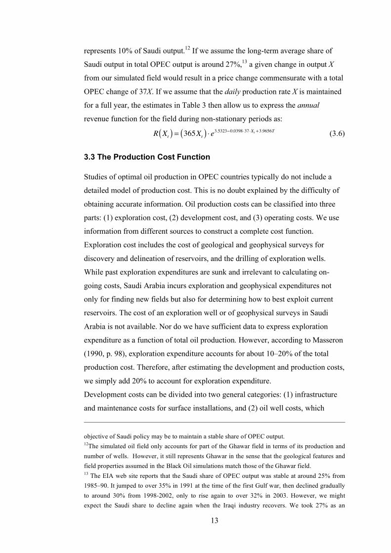
represents 10% of Saudi output.12 If we assume the long-term average share of
Saudi output in total OPEC output is around 27%,13 a given change in output X
from our simulated field would result in a price change commensurate with a total
OPEC change of 37X. If we assume that the daily production rate X is maintained
for a full year, the estimates in Table 3 then allow us to express the annual
revenue function for the field during non-stationary periods as:
R Xt( ) = 365X
t( ) ! e3.5323"0.0398!37!Xt +3.9656T (3.6)
3.3 The Production Cost Function
Studies of optimal oil production in OPEC countries typically do not include a
detailed model of production cost. This is no doubt explained by the difficulty of
obtaining accurate information. Oil production costs can be classified into three
parts: (1) exploration cost, (2) development cost, and (3) operating costs. We use
information from different sources to construct a complete cost function.
Exploration cost includes the cost of geological and geophysical surveys for
discovery and delineation of reservoirs, and the drilling of exploration wells.
While past exploration expenditures are sunk and irrelevant to calculating on-
going costs, Saudi Arabia incurs exploration and geophysical expenditures not
only for finding new fields but also for determining how to best exploit current
reservoirs. The cost of an exploration well or of geophysical surveys in Saudi
Arabia is not available. Nor do we have sufficient data to express exploration
expenditure as a function of total oil production. However, according to Masseron
(1990, p. 98), exploration expenditure accounts for about 10–20% of the total
production cost. Therefore, after estimating the development and production costs,
we simply add 20% to account for exploration expenditure.
Development costs can be divided into two general categories: (1) infrastructure
and maintenance costs for surface installations, and (2) oil well costs, which
objective of Saudi policy may be to maintain a stable share of OPEC output. 12The simulated oil field only accounts for part of the Ghawar field in terms of its production and number of wells. However, it still represents Ghawar in the sense that the geological features and field properties assumed in the Black Oil simulations match those of the Ghawar field. 13 The EIA web site reports that the Saudi share of OPEC output was stable at around 25% from 1985–90. It jumped to over 35% in 1991 at the time of the first Gulf war, then declined gradually to around 30% from 1998-2002, only to rise again to over 32% in 2003. However, we might expect the Saudi share to decline again when the Iraqi industry recovers. We took 27% as an
14
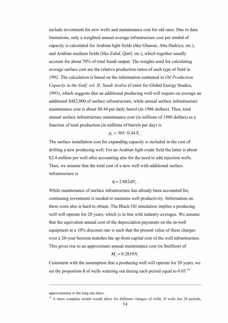
include investment for new wells and maintenance cost for old ones. Due to data
limitations, only a weighted annual average infrastructure cost per mmbd of
capacity is calculated for Arabian light fields (like Ghawar, Abu Hadriya, etc.),
and Arabian medium fields (like Zuluf, Qatif, etc.), which together usually
account for about 70% of total Saudi output. The weights used for calculating
average surface cost are the relative production ratios of each type of field in
1992. The calculation is based on the information contained in Oil Production
Capacity in the Gulf, vol. II: Saudi Arabia (Center for Global Energy Studies,
1993), which suggests that an additional producing well will require on average an
additional $482,000 of surface infrastructure, while annual surface infrastructure
maintenance cost is about $0.44 per daily barrel (in 1986 dollars). Thus, total
annual surface infrastructure maintenance cost (in millions of 1986 dollars) as a
function of total production (in millions of barrels per day) is
µt= 365 !0.44X
t.
The surface installation cost for expanding capacity is included in the cost of
drilling a new producing well. For an Arabian light crude field the latter is about
$2.4 million per well after accounting also for the need to add injection wells.
Thus, we assume that the total cost of a new well with additional surface
infrastructure is
! = 2.882dNt.
While maintenance of surface infrastructure has already been accounted for,
continuing investment is needed to maintain well productivity. Information on
these costs also is hard to obtain. The Black Oil simulation implies a producing
well will operate for 20 years, which is in line with industry averages. We assume
that the equivalent annual cost of the depreciation payments on the in-well
equipment at a 10% discount rate is such that the present value of these charges
over a 20-year horizon matches the up-front capital cost of the well infrastructure.
This gives rise to an approximate annual maintenance cost (in $million) of
Mt= 0.2819N
t
Consistent with the assumption that a producing well will operate for 20 years, we
set the proportion δ of wells watering out during each period equal to 0.05.14
approximation to the long run share. 14 A more complete model would allow for different vintages of wells. If wells last 20 periods,

15
Production cost refers to operation costs and reservoir engineering costs that vary
with output. These include the expenditures on manpower and other variable
production costs. According to a report from the EIA (1996), variable operating
expenses per barrel range from $0.25 to $1.00, depending on the rate of
extraction. The EIA provides the following estimated functional relationship
between annual production (365X) and variable operating costs15:
V
t= 0.7714(365X
t)!0.2423 (3.7)
Water must be injected into the reservoir to maintain the reservoir fluid pressure.
We use the water injection costs to capture the reservoir engineering costs.
Industry studies indicate that these costs are on the order of about $0.20 per daily
barrel of water per day for Saudi Arabia. This leads to an annual water injection
cost (in millions of dollars) of
!t= 365 "0.20W
t
Summing these components, and multiplying by 1.2 to account for exploration
expenditure, the resulting oil production cost (in $million) per year becomes
Ct=1.2{µ +V
t(365X)+!
t+M
t+"
t} =1.2{365 # 0.44X
t+
(0.7714(365Xt)-0.2423
)$ (365Xt)+ 365 $ (0.2W
t)+ 0.2819N
t+ 2.882dN
t}
(3.8)
where X, W, N, dN follow the same notation as in (2.1). The water injection rate
(W) was modeled as a function of the number of producing wells (N) and the daily
production rate (X) in section 3.1.
3.4 Summary
The results derived in this section can be summarized by restating the dynamic
programming model using the estimated functions. Notice that the first two
equations in the constraints represent the state transition equations in the model.
vtN
t,CP
t( ) = MaxXt ,dNt { 365Xt( ) ! e3.5323"0.0398#37#Xt +3.9656t -1.2{(0.44 # 365)Xt
+(0.7714(365Xt)–0.2423
)# (365Xt)+ 365 # (0.2W
t)+ 0.2819N
t+ 2.882dN
t}
+$vt+1 Nt+1,CPt+1( )}
(3.9)
subject to
however, this would add 20 new state variables. In addition, we would need to know the vintages of current wells in order to solve the model and this information was not available to us. 15 The EIA’s Estimator database contains field and production characteristics for eight geological plays (a group of discovered and/or undiscovered fields with similar geological, geographic, and temporal characteristics) as well as varying field sizes based on expected ultimate recovery.
16
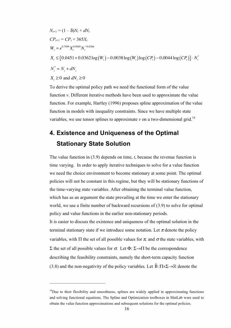
Nt+1 = (1 – δ)Nt + dNt
CPt+1 = CPt + 365Xt
Wt= e
0.7999Xt
0.9509N
t
*0.0306
Xt! 0.0451+ 0.0362 log W
t( ) " 0.0038 log Wt( ) log CPt( ) " 0.0044 log CP
t( ){ } # Nt
*
N
t
*= N
t+ dN
t Xt! 0 and dN
t! 0
To derive the optimal policy path we need the functional form of the value
function v. Different iterative methods have been used to approximate the value
function. For example, Hartley (1996) proposes spline approximation of the value
function in models with inequality constraints. Since we have multiple state
variables, we use tensor splines to approximate v on a two-dimensional grid.16
4. Existence and Uniqueness of the Optimal
Stationary State Solution
The value function in (3.9) depends on time, t, because the revenue function is
time varying. In order to apply iterative techniques to solve for a value function
we need the choice environment to become stationary at some point. The optimal
policies will not be constant in this regime, but they will be stationary functions of
the time-varying state variables. After obtaining the terminal value function,
which has as an argument the state prevailing at the time we enter the stationary
world, we use a finite number of backward recursions of (3.9) to solve for optimal
policy and value functions in the earlier non-stationary periods.
It is easier to discuss the existence and uniqueness of the optimal solution in the
terminal stationary state if we introduce some notation. Let π denote the policy
variables, with Π the set of all possible values for π, and σ the state variables, with
Σ the set of all possible values for σ. Let Φ: Σ→Π be the correspondence
describing the feasibility constraints, namely the short-term capacity function
(3.8) and the non-negativity of the policy variables. Let !̂ :Π×Σ→ denote the
16Due to their flexibility and smoothness, splines are widely applied in approximating functions and solving functional equations. The Spline and Optimization toolboxes in MatLab were used to obtain the value function approximations and subsequent solutions for the optimal policies.

17
estimated profit function (“∧” stands for the estimated function) r – c in (2.1). Use
M to denote the state transition function, M: Π×Σ → Σ described in (3.9).
Once the choice environment is stationary, the dynamic programming model (3.9)
can be summarized as (4.1) with an operator, T, on the space of continuous and
bounded functions.
T ! v( ) " t( ) = max
#t$% "
t( )&̂ #
t,"
t( ) + 'v "t+1( ){ } (4.1)
A reasonably straight-forward application of Theorem 4.6 in Stokey, Lucas and
Prescott (1989) implies that T as defined in (4.1) has a unique fixed point
v* ∈ (σ) such that for all v0 ∈ (σ),
T
nv
0! v * " # n
v0! v * , n =1,2,…
Moreover, given v*, the optimal policy correspondence P: Σ→Π, defined as
P(! ) = " # $ !( ) : v * !( ) = %̂ " ,!( ) + &v * M " ,!( )( ){ }
is compact-valued and upper hemi-continuous. The existence of a fixed point for
the operator T justifies using iterative methods to approximate the stationary state
value function. The theorem from Stokey, Lucas and Prescott (1989) also provides
a bound on the rate of convergence.
Using Theorem 4.7 in Stokey, Lucas and Prescott (1989), one can also show that,
for our functional forms, v* is strictly decreasing in CP. We verify that the
calculated value functions in the next section are consistent with this result.
5. Simulation Results
This section presents numerical approximations to the value function and the
optimal policy paths under five scenarios. Scenario I assumes that the discount
factor is 0.9 (discount rate ! 0.1) and the states with a stationary demand curve
begin in 2045. Scenario II keeps the beginning stationary state date as 2045, but
sets the discount factor to 0.7 to capture Saudi Arabia’s heavy reliance on its oil
income. The difference in outcome between scenarios I and II can be used to
gauge the effect the discount factor has on the solution.
Scenarios III and IV retain β = 0.9 but study the impact of an anticipated
technology breakthrough that significantly reduces the cost of solar energy or
other backstop technologies for generating electricity and using it to power
vehicles. Only the revenue function is affected by such a shock to oil demand. In
18
scenario III, the alternative technology is assumed to become competitive with oil
in 2036 and continue to improve and reduce oil demand over a ten-year period. To
be specific, we assume that by the end of the transition period, the inverse demand
equation will have contracted proportionately by a factor of 2 so (3.5) becomes
log2Pt= !0 +!12yt +!2T
with the reduction in demand occurring uniformly over the transition period. The
transition pattern is purely hypothetical. We are interested in how expectations of
such a transition would affect Saudi Arabia’s oil production policy in the short to
medium term.
Scenario IV repeats scenario III with a more optimistic projection that implies the
technological breakthrough will occur in 2026 instead of 2036. This allows us to
see how the expected timing of such a shock affects Saudi’s oil production
decisions. Changing the timing of the solar technology shock from 2036 to 2026
does not effect the value function v* in the stationary state, although the values of
the state variables when the stationary state begins would be different.
Finally, scenario V repeats scenario III but varies the ratio of total OPEC to Saudi
production. Specifically, we now take the ratio of OPEC production to production
from our simulated field to be 40 from 1986-1990 (implying a Saudi share of
OPEC production of around 25%), 35 in 1991 (implying a Saudi share of around
28.5%), and 31 thereafter (corresponding to a Saudi share of around 32.25%).
Figures 1–4 graph the tensor spline numerical approximations to the value
function in the terminal stationary state as a function of the number of wells N and
cumulative production to date CP.17 Contour levels of the function are included on
the floor of the 3-D space to help the reader understand the shape of the surface.
The time-varying value functions in earlier periods are derived using backward
recursion. From the shape of these surfaces it is clear that once cumulative
production from this simulated field reaches around 20 billion barrels
(corresponding to overall Saudi production of 200 billion barrels), Saudi
production will begin to fall off rather sharply.
17 Recall that the stationary v* is the same in scenarios III and IV. It may also be worth remarking that the ranges of values for N and CP for which v* has been graphed are larger than encountered in the time period that we subsequently examine. This has been done for the technical reason that the ranges of values have to be large enough to ensure the maximizing dN = 0 for large values of N in the approximation region. If this were not the case, we could not use an existing approximation to v* to evaluate the right hand side of the functional equation (3.9).

19
Fig. 1 Stationary value function for β = 0.9 and stationary terminal demand
Fig. 2 Stationary value function for β = 0.7 and stationary terminal demand

20
Fig. 3 Stationary value function in scenarios III and IV with backstop technology that reduces
demand in the stationary state
Fig. 4 Stationary value function with backstop and changed Saudi share of OPEC output
21
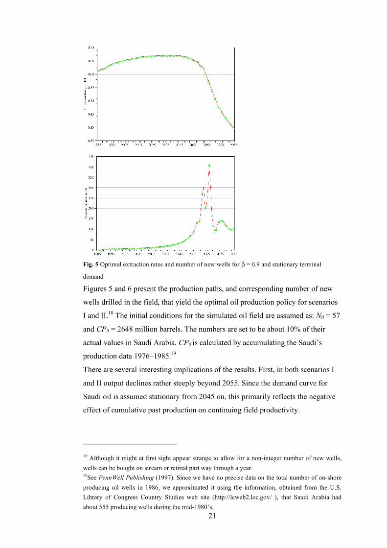
Fig. 5 Optimal extraction rates and number of new wells for β = 0.9 and stationary terminal
demand
Figures 5 and 6 present the production paths, and corresponding number of new
wells drilled in the field, that yield the optimal oil production policy for scenarios
I and II.18 The initial conditions for the simulated oil field are assumed as: N0 = 57
and CP0 = 2648 million barrels. The numbers are set to be about 10% of their
actual values in Saudi Arabia. CP0 is calculated by accumulating the Saudi’s
production data 1976–1985.19
There are several interesting implications of the results. First, in both scenarios I
and II output declines rather steeply beyond 2055. Since the demand curve for
Saudi oil is assumed stationary from 2045 on, this primarily reflects the negative
effect of cumulative past production on continuing field productivity.
18 Although it might at first sight appear strange to allow for a non-integer number of new wells, wells can be bought on stream or retired part way through a year. 19See PennWell Publishing (1997). Since we have no precise data on the total number of on-shore producing oil wells in 1986, we approximated it using the information, obtained from the U.S. Library of Congress Country Studies web site (http://lcweb2.loc.gov/ ), that Saudi Arabia had about 555 producing wells during the mid-1980’s.
22
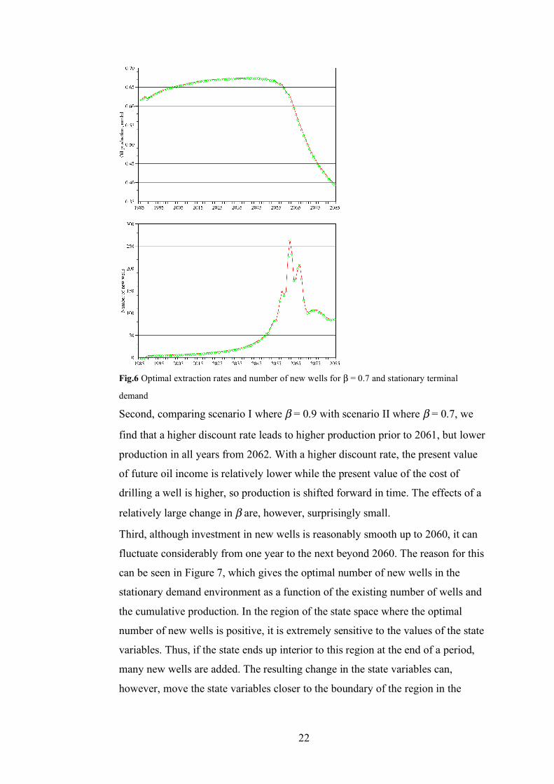
Fig.6 Optimal extraction rates and number of new wells for β = 0.7 and stationary terminal
demand
Second, comparing scenario I where β = 0.9 with scenario II where β = 0.7, we
find that a higher discount rate leads to higher production prior to 2061, but lower
production in all years from 2062. With a higher discount rate, the present value
of future oil income is relatively lower while the present value of the cost of
drilling a well is higher, so production is shifted forward in time. The effects of a
relatively large change in β are, however, surprisingly small.
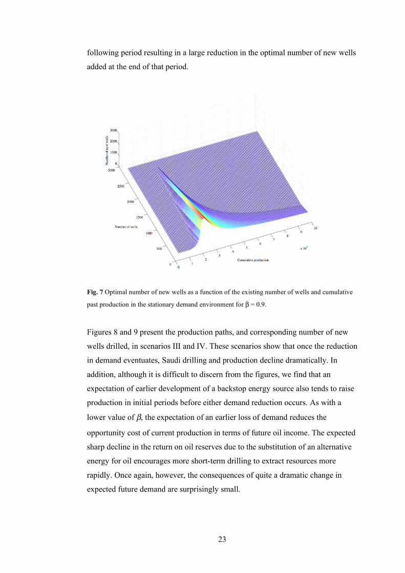
Third, although investment in new wells is reasonably smooth up to 2060, it can
fluctuate considerably from one year to the next beyond 2060. The reason for this
can be seen in Figure 7, which gives the optimal number of new wells in the
stationary demand environment as a function of the existing number of wells and
the cumulative production. In the region of the state space where the optimal
number of new wells is positive, it is extremely sensitive to the values of the state
variables. Thus, if the state ends up interior to this region at the end of a period,
many new wells are added. The resulting change in the state variables can,
however, move the state variables closer to the boundary of the region in the
23
following period resulting in a large reduction in the optimal number of new wells
added at the end of that period.
Fig. 7 Optimal number of new wells as a function of the existing number of wells and cumulative
past production in the stationary demand environment for β = 0.9.
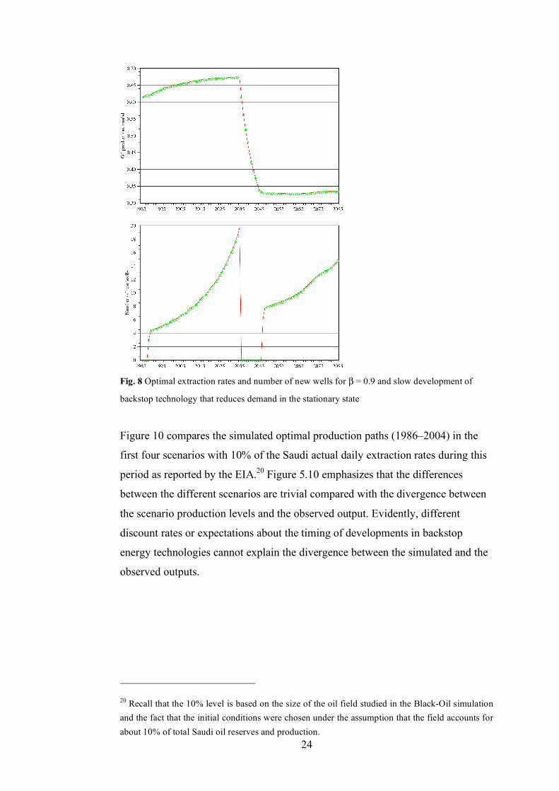
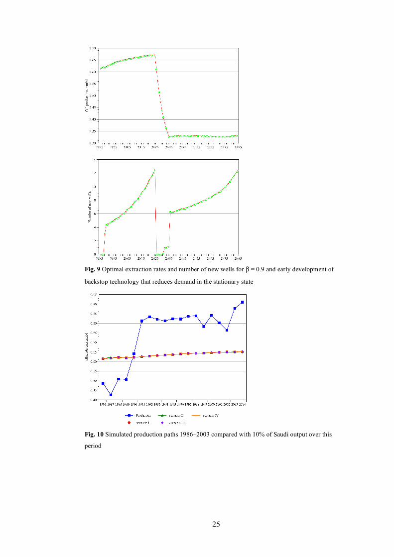
Figures 8 and 9 present the production paths, and corresponding number of new
wells drilled, in scenarios III and IV. These scenarios show that once the reduction
in demand eventuates, Saudi drilling and production decline dramatically. In
addition, although it is difficult to discern from the figures, we find that an
expectation of earlier development of a backstop energy source also tends to raise
production in initial periods before either demand reduction occurs. As with a
lower value of β, the expectation of an earlier loss of demand reduces the
opportunity cost of current production in terms of future oil income. The expected
sharp decline in the return on oil reserves due to the substitution of an alternative
energy for oil encourages more short-term drilling to extract resources more
rapidly. Once again, however, the consequences of quite a dramatic change in
expected future demand are surprisingly small.
24
Fig. 8 Optimal extraction rates and number of new wells for β = 0.9 and slow development of
backstop technology that reduces demand in the stationary state
Figure 10 compares the simulated optimal production paths (1986–2004) in the
first four scenarios with 10% of the Saudi actual daily extraction rates during this
period as reported by the EIA.20 Figure 5.10 emphasizes that the differences
between the different scenarios are trivial compared with the divergence between
the scenario production levels and the observed output. Evidently, different
discount rates or expectations about the timing of developments in backstop
energy technologies cannot explain the divergence between the simulated and the
observed outputs.
20 Recall that the 10% level is based on the size of the oil field studied in the Black-Oil simulation and the fact that the initial conditions were chosen under the assumption that the field accounts for about 10% of total Saudi oil reserves and production.
25
Fig. 9 Optimal extraction rates and number of new wells for β = 0.9 and early development of
backstop technology that reduces demand in the stationary state
Fig. 10 Simulated production paths 1986–2003 compared with 10% of Saudi output over this
period

26
Fig. 11 Revenue and marginal revenue functions for output from the simulated field
Figure 11 suggests an explanation for the small magnitude of the effects (in early
periods) of changes in β or the timing of developments in backstop technologies.21
This shows the revenue and marginal revenue functions for the simulated oil field
in the terminal stationary regime.22 Revenue shows a sharp peak around an output
of 0.68, which corresponds to overall Saudi output of 6.8 mmbd. Since the
marginal revenue curve is steep, small shifts in marginal cost, including the
opportunity cost of mining today rather than leaving resource to be exploited in
the future, lead to small changes in the optimal output. Thus, the output path is
very smooth until the cost changes from one period to the next get large (after
2055 in scenarios I and II). In addition changes in factors that affect costs have
little effect on optimal output prior to 2055.
21 Scenarios I and II compare two different constant values for β rather than a time path that changes from year to year. If β could vary over time, however, an extremely large number of paths could be examined. To check whether a time varying β would alter our conclusions, we examined two additional scenarios based on scenario III. In one of them we assumed β was 0.7 for the first ten years but then 0.9 (as in scenario III) for the remaining periods, while the other examined the reverse case where β was 0.9 for ten years, but then falls to 0.7 for the remaining periods. In both cases, we assumed a slow development of the backstop as in scenario III. These different time paths for β had very little effect on the solution. We did not include these more complicated scenarios in the paper to save space, but the results are available from the authors upon request. 22 The shifts in the demand curve in earlier periods essentially re-scale the y-axis since they multiply revenue and marginal revenue by the same constant.

27
By contrast, the effect of the introduction of the backstop technology is large
because it greatly affects the output corresponding to maximum revenue. Scenario
V further illustrates this point. A critical determinant of the output corresponding
to peak revenue is the Saudi share of total OPEC output. Scenario V varies the
Saudi share of OPEC output while otherwise retaining the discount rate and
backstop technology assumptions of scenario III. Specifically, we now take the
ratio of OPEC production to production from our simulated field to be 40 from
1986-1990, 35 in 1991, and 31 thereafter. These values approximate the actual
historical ratio of OPEC to Saudi production from 1986-2004. Figure 12 graphs
the resulting optimal levels of output and new wells drilled. As in Figure 10, we
have included 10% of actual Saudi output over the period 1986-2004. The
increase in world demand from rapid economic growth may explain further
increases in Saudi output from 2003 and beyond.
Fig.12 Optimal extraction rates and number of new wells for β = 0.9, slow development of
backstop technology and increased Saudi share of OPEC production
Figure 13 compares the oil price paths in each of the five scenarios with the actual
path of the real fob price for US imports of Saudi oil in 1986 dollars (using the US

28
CPI as deflator).23 Since the model is deterministic, it is not surprising that the
actual price path is more volatile than the simulated price paths. The apparent flat
trend in the actual price path, however, is inconsistent with the rising trend in the
simulated paths.24
Fig.13 Actual real Saudi oil prices compared with the simulation outcomes
The actual price path could reflect a slower growth in the world economy, and
hence in energy demand, in the 1990’s than the simulated trajectories using the
OMS model. Of particular interest in this regard is the observation from Figure 12
that the scenario V model approximates the quantity of Saudi output much better
than it approximates the real price in Figure 13. Observing a similar quantity at a
lower price suggests that demand is not as high as the model assumes. If a shift in
the demand curve does explain the price discrepancy, the model suggests that it
shifts in a way that does not greatly alter the level of output where marginal
revenue approximates marginal cost (including the opportunity cost of mining
today at the expense of higher mining costs in the future). Also of interest is that
23 The oil price data were obtained from the EIA web site and the CPI from the FRED database at the Federal Reserve Bank of St Louis. 24 Although the exponentially rising trend of the simulated price path is consistent with the prediction of the simplest version of Hotelling’s model (Prato 1997, p. 140 or Neher 1990, p. 95), in later periods, where cumulative production begins to strongly affect costs, the prices do not rise at a constant percentage rate. Solow and Wan (1976) and Heal (1976) were the first papers to allow extraction costs to depend on cumulative past exploitation. Part of their motivation was the observation that, contrary to the predictions of the simplest Hotelling model, real prices of natural resource commodities show a long-term decline. Slade and Thille (1997) observe that factors such as large unanticipated discoveries, technical change that lowers mining costs, and the development of substitute materials that reduce demand could also explain declining resource prices.

29
the recent rise in oil prices on the heals of dramatically growing demand from
China, India and elsewhere has raised real prices much closer to the path forecast
by the model scenarios.
Another explanation for the divergence between the model and actual outcome is
that the Saudi decision makers do not have profit maximization as their objective.
The model could nevertheless prove useful in such a circumstance. If we assume
that deviations between the actual and the simulated production paths represent
the pursuit of other objectives, the simulation results would reveal the potential
costs of pursuing those objectives in terms of foregone profits.
In order to investigate this possibility, we further modified scenario V to allow the
observed output, and corresponding real price, to be chosen as optimal.
Specifically, we altered the demand curve intercept in (3.5) in years 1986–2004 to
ensure that the curve passed through the observed quantity and real price pair.25
Without making this change, the revenues earned in scenario V, for example,
could be much larger than observed not because chosen output is not profit
maximizing but rather because the assumed level of demand is unrealistic.
Table 4 Observed and simulated profit-maximizing production, prices and revenues (millions of
1986 dollars), 1986–2004
Year Actual output Simulated
output
Actual real
price
Simulated
real price
Revenue
difference
1986 4.8700 5.4430 11.36 10.37 -2.0% 1987 4.2650 5.5540 14.59 11.88 -5.7% 1988 5.0860 5.4630 11.27 10.61 -1.1% 1989 5.0640 5.6190 14.40 13.19 -1.6% 1990 6.4100 5.7740 17.08 18.90 0.3% 1991 8.1150 7.2480 11.77 13.28 -0.8% 1992 8.3317 7.2180 12.38 14.20 0.6% 1993 8.1978 7.0650 10.45 12.02 0.9% 1994 8.1200 7.0530 10.44 11.91 0.9% 1995 8.2312 7.2650 13.36 15.05 0.6% 1996 8.2181 7.2700 13.47 15.14 0.6% 1997 8.3620 7.0820 10.35 12.12 0.8% 1998 8.3889 6.4770 5.96 7.55 2.3% 1999 7.8334 7.1100 11.61 12.70 0.8% 2000 8.4038 7.3820 15.67 17.78 0.4% 2001 8.0311 7.1310 11.75 13.13 0.8% 2002 7.6344 7.2730 14.58 15.24 0.4% 2003 8.7750 7.3740 14.91 17.73 0.1% 2004 9.1008 7.5540 19.78 23.93 -0.5%
25 Beyond 2004, we assumed that the demand curve gradually reverted to the scenario V one.
30
Table 4 compares the actual outputs and prices with the profit maximizing levels
under this altered scenario. The final column of the table gives the difference
between the actual and the simulated profit maximizing revenues as a percentage
of the latter. The first point to note is that the simulated profit-maximizing output
tends to increase less, and the real price more, than the actual levels post-1990.
This could reflect, for example, a price stabilization objective of Saudi decision-
makers. The second observation, however, is that the deviation between the actual
and the profit-maximizing revenue is quite small. Third, the actual revenue
exceeds the simulated revenue in 1990 and from 1992-2003. Evidently, even
though revenue in those years is higher than the simulated value, the present value
of costs on the actual path must also be higher. These additional costs could take
the form not only of higher drilling costs for additional new wells, for example,
but also anticipated effects of higher output on future production costs. By
definition, the simulated path maximizes the net present value of profits taking
account also of all the effects of current production on current and future costs.
6. Conclusions
We proposed and illustrated an integrated economic and engineering analysis of
the dynamic production decisions for an idealized oil field approximating the
largest oil field in Saudi Arabia – Ghawar. The Workbench Black Oil Simulator
model was used to characterize the reservoir engineering aspects of the problem.
Our analysis incorporates a game theoretical structure of the world oil market
(taking Saudi Arabia as a Stackelberg leader) using the Oil Market Simulation
model developed by the EIA. The results of the optimal production model
approximate actual Saudi Arabia extraction rates.
Comparing results under different scenarios helped elucidate influences on Saudi
Arabia’s investment and production decisions. In particular, we found that
changes in the time discount factor or the timing of developments in backstop
technologies had a surprisingly small effect on near-term production decisions.
The reason is that the marginal revenue curve is very steep, so small shifts in
marginal cost, including the opportunity cost of producing now rather than later,
lead to small changes in profit maximizing output. On the other hand, factors that
change the marginal revenue curve, including a change in Saudi share in OPEC
output, can produce significant changes in the maximizing level of output.

31
Although the model approximates Saudi Arabia’s oil production decisions, we
have made many simplifications that could be relaxed in future work. The most
important is that the assumption of perfect knowledge and foresight is unrealistic.
Examining a number of different scenarios demonstrates the range of possible
outcomes. However, as Powell (1990) pointed out, a decision maker who knows
the environment is uncertain would take that into account by choosing production
and investment paths to maximize the expected present value of profits. The
model could be extended to encompass a stochastic demand environment and
randomize the timing of the breakthrough in backstop technology. In this regard, a
rather interesting feature of the value function graphed in Figures 1–4 is that it is
convex over part of its domain. Where the value function is concave, the decision
maker would be willing to take a lower expected value of profits if that also
allowed profits to be less variable. If the value function is locally convex,
however, the decision maker may behave as if he were not so risk averse.
A second modification would involve using a multi-level optimization (MLO)
approach instead of modeling Saudi Arabia’s oil production decision purely as
maximization of the present value of its profits. This would allow a trade-off
between profit maximization and other motivations of the Saudi Arabian
government. Islam (1998) provides a good example of using MLO to model
energy plans involving both the private sector and the government.
Last, but not least, while using the OMS model simplified our task, this may have
affected the accuracy of the model. A more ambitious approach would incorporate
strategic behavior directly into the dynamic optimization model.
7. Appendix – The Workbench Black Oil Simulation
Strategy
The parameters are set to mimic the rock, fluid, and fluid/rock interaction
properties typical of the Ghawar field, which is a Jurassic Arab-D calcarenitic
limestone formation more akin to highly porous and permeable sandstone than
fractured limestone (geological information can be found in Afifi (2005) or
Durham (2005)). The reservoir gross thickness is about 75 meters. The dip of the
formation varies from 0 degrees at the crest to about 5 degrees on the flank.
The typical operational procedure is to drill producing wells downdip of the crest
and injection wells for peripheral water injection below the oil/water contact. If
32
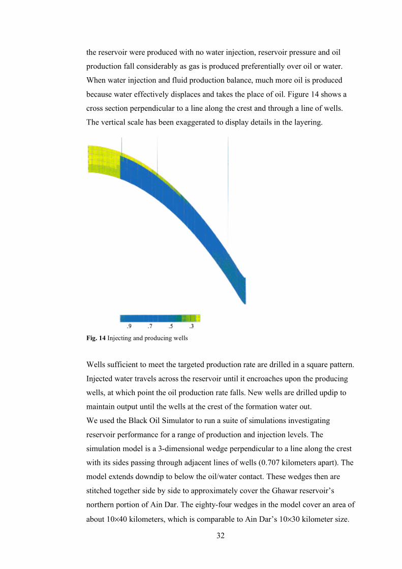
the reservoir were produced with no water injection, reservoir pressure and oil
production fall considerably as gas is produced preferentially over oil or water.
When water injection and fluid production balance, much more oil is produced
because water effectively displaces and takes the place of oil. Figure 14 shows a
cross section perpendicular to a line along the crest and through a line of wells.
The vertical scale has been exaggerated to display details in the layering.
Fig. 14 Injecting and producing wells
Wells sufficient to meet the targeted production rate are drilled in a square pattern.
Injected water travels across the reservoir until it encroaches upon the producing
wells, at which point the oil production rate falls. New wells are drilled updip to
maintain output until the wells at the crest of the formation water out.
We used the Black Oil Simulator to run a suite of simulations investigating
reservoir performance for a range of production and injection levels. The
simulation model is a 3-dimensional wedge perpendicular to a line along the crest
with its sides passing through adjacent lines of wells (0.707 kilometers apart). The
model extends downdip to below the oil/water contact. These wedges then are
stitched together side by side to approximately cover the Ghawar reservoir’s
northern portion of Ain Dar. The eighty-four wedges in the model cover an area of
about 10×40 kilometers, which is comparable to Ain Dar’s 10×30 kilometer size.

33
The main portion of Ghawar is about 180 kilometers wide. Reservoirs that are
close by, and which are comparable to the representative reservoir we model,
include Abqaiq (15×40 kilometers) and Harmaliyah (8×15 kilometers).
The output of the simulations consists of time series of the pressure and the
amount of oil, gas, and water present at selected points in the reservoir (the “state”
of the reservoir) and the production rates of oil, gas, and water out of, and
injection rates of water into, each of the wells. The amount of oil, gas, and water
present in the reservoir around a well, and the pressure in the well, determine the
ability of the well to produce or accept injected fluids. While well performance
can be taken as a measure of the local state, it does not reflect the state of the
entire reservoir. For this reason, correlating the performance of the producing
wells against that of the injection wells is not always successful.
The scheduling of the wells in each wedge takes place as follows. The model has
five producing and two injection wells. Both of the injectors and the first
producing well (the one lowest on the structure) are drilled at the same time and
thus represent the initial investment. Subsequent capital investments are made as
the additional producers are drilled following watering out of previous wells. The
fifth producer well is drilled on the crest. Production and injection were balanced
in the sense that any changes to the rates were made to the producers and injectors
at the same time. The length of each simulation is 23 years.
Fig. 15 Typical well production schedule when the production rate is 5% of reserves per year

34
In general, the higher the target production rate, the quicker the wells have to be
drilled. In order to produce 5% of total reserves per year, only one well is needed.
As each producing well waters out, one new well is drilled until the third well
waters out. The deliverability of the next to highest well is insufficient to meet the
target, however, so the fourth and fifth wells have to be drilled at the same time.
At the highest target (9% of reserves per year), only the first well can meet the
target by itself. When that well waters out, all the remaining wells have to be
drilled. At the intermediate targets (6%, 7%, 8% of reserves per year), the results
lie between these two extremes. The capital investment schedule for each of these
cases would be different, because of the different schedules for drilling the wells.
There is a trade-off between deferring capital investment at lower production rates
and the loss of revenue in present value terms.
Additional sets of simulations were performed to examine the effects of
production rates on well requirements and water injection. Each simulation was
started at one of the five levels of production target just described. After a length
of time at that initial rate, the rate was either increased to the next higher, or
decreased to the next lower level of production target and then maintained at that
rate for the remainder of the time. Simulations were made with the rate change at
two, four, and six years. In all, twenty-nine simulations were run.
8. References
Adelman, M. A. (1993a), The Economics of Petroleum Supply, Cambridge: The MIT Press.
Adelman, M. A. (1993b), “Modelling World Oil Supply,” The Energy Journal, 14, 1-31.
Afifi, A.M. (2005), “Ghawar: The Anatomy of the World’s Largest Oil Field,” Search and
Discovery article 20026, January 2005, available at http://www.searchanddiscovery.com/
Askari, H. (1991), “Saudi Arabia’s Oil Policy: Its Motivation and Impact,” in: Wilfrid Kohl (ed)
After the Oil Price Collapse: OPEC, the United States, and the World Market, Baltimore: The
Johns Hopkins University Press.
Azzam, H. T. (1993), Saudi Arabia: Economic Trends, Business Environment, and Investment
Opportunity, London: Euromoney Books.
Benkherouf, L. (1994), “A Generalized Oil Exploration Problem,” European Journal of
Operational Research, 73, 423-429.
Berg, Elin, Snorre Kverndokk and Knut Einar Rosendahl (1997), “Gains from Cartelisation in the
Oil Market,” Energy Policy, 25(13), 1075-1091.
Center for Global Energy Studies (1993), Oil Production Capacity in the Gulf, Volume 2.
Cremer, J., and D. Salehi-Isfahani (1989), “The Rise and Fall of Oil Prices: A Competitive View,”
Annales D’Economie et de Statistique, 15/16, 427-454.
35
Cremer, J., and D. Salehi-Isfahani (1991), Models of the World Oil Market, London: Harwood
Academic Publishers.
Dahl, C., and M. Yucel (1991), “Testing Alternative Hypotheses of Oil Market Behavior,” The
Energy Journal, 12, 117-39.
Durham, L. (2005), “Saudi Arabia’s Ghawar Field: The Elephant of All Elephants,” AAPG
Explorer, January 2005, available at http://www.aapg.org/explorer/2005/01jan/ghawar.cfm
Energy Information Administration (1996), Oil Production Capacity Expansion Costs for the
Persian Gulf, DOE/EIA-TR/0606, Washington, D. C.
Energy Information Administration (1996), The 1992 Oil Market Simulation Model, Washington,
D. C.
Energy Information Administration (1996), International Energy Outlook, DOE/EIA-0484,
Washington, D.C.
Feraille, Mathieu, Emmanual Manceau, Isabelle Zabalza-Mezghani, Frederic Roggero, Lin-Ying
Hu and Leandro Costa Reis (2003), “Integration of dynamic data in a amture field reservoir model
to reduce the uncertainty on production forecasting”, paper presented at the AAPG Annual
Convention, Salt Lake City, Utah, May 11-14.
Fousekis, P., and S. E. Stefanou (1996), “Capacity Utilization Under Dynamic Profit Maximum”,
Empirical Economics, 21, 335-359.
Gately, D. (1984). “A Ten-year Retrospective: OPEC and the World Oil Market.” Journal of
Economic Literature 22(3):1100-1114.
Gately, D. (2004), “OPEC’s Incentives for Faster Output Growth,” The Energy Journal 25(2): 75–
96.
Good, D. H., M. I. Nadiri, and R. C. Sickles, (1997) “Index Number and Factor Demand
Approaches to the Estimation of Productivity,” Chapter 1 of the Handbook of Applied Economics,
Volume II-Microeconometrics, with D. Good and M. I. Nadiri, edited by M. H. Pesaran and P.
Schmidt, Oxford: Basil Blackwell, 1997, 14-80, reprinted as National Bureau of Economic
Research Working Paper # 5790, 1996, Cambridge, MA.
Gong, Byeong-Ho, (1990), "Finite Sample Properties of Stochastic Frontier Models Using Panel
Data," Journal of Productivity Analysis 1, l990, 229-261.
Griffin, J. M. (1977), “The Econometrics of Joint Production: Another Approach,” Review of
Economics and Statistics, 109, 389-397
Griffin, J. M. (1978), “Joint Production Technology: the Case of Petrochemicals,” Econometrica,
46, 379-396.
Griffin, J. M. (1985),”OPEC Behavior: A Test of Alternative Hypotheses,” American Economic
Review, 75, 954-63.
Griffin, J. M., and Nielson (1994), “The 1985-86 Price Collapse and Afterwards: What Does
Game Theory Add?,” Economic Inquiry, October, 543-61.
Guilkey, D. K., C. A. K. Lovell, and R. C. Sickles (1983), "A Comparison of the Performance of
Three Flexible Functional Forms," International Economic Review 24, l983, 59l-6l6.

36
Hartley, P. R. (1996), “Value Function Approximation in the Presence of Uncertainty and
Inequality Constraints: an Application to the Demand for Credit Cards,” Journal of Economic
Dynamics and Control, 20: 63-92.
Heal, G (1976), “The Relationship between Price and Extraction Cost for a Resource with a
Backstop Technology,” Bell Journal of Economics, Volume 7(2): 371–378.
Hotelling, H. (1931), “The Economics of Exhaustible Resources,” Journal of Political Economy,
39, 137-175.
Islam, S. M. N. (1998), Mathematical Economics of Multi-level Optimization: Theory and
Application, New York: Physica-Verlag.
Jensen, J. (2003), “The LNG Revolution” Energy Economics Volume 24, Issue 2,1-45.
Khadduri, B. (1996), “Oil and politics in the Middle East security dialogue,” Security Dialogue,
27, 155-166.
Lohrenz, P. E., and A. J. Bailey (1995), “Evidence and results of present value maximization for
oil and gas development projects,” Proceedings, Hydrocarbon Economics and Evaluation
Symposium, Dallas, 163-177.
Masseron, J. (1990), Petroleum Economics, Institut Français du Pétrole Publications (Distributed
in the United States by Gulf Publishing Company).
Maycock, P.D. “PV Review: World Solar PV Market Continues Explosive Growth,” REFocus,
September/October, 2005, 18–22.
National Renewable Energy Laboratory (2007), Photovoltaic Research, http://www.nrel.gov/pv/ ,
last accessed July 12, 2007.
Neher, P. A. (1990), Natural Resource Economics: Conservation and Exploitation, Cambridge:
Cambridge University Press.
Nemet, G. F. (2006), “Beyond the learning curve: factors influencing cost reductions in
photovoltaics,” Energy Policy, 34, 3218–3232.
PennWell Publishing Company (1997), Energy Statistics Sourcebook, 12th ed.
Powell, S. (1990), “The Target Capacity-Utilization Model of OPEC and the Dynamics of the
World Oil Market,” The Energy Journal, 11, 27-61.
Prato, T. (1997), Natural Resource and Environmental Economics, Iowa State University Press,
Ames.
Quandt, W. B. (1982), “Saudi Arabia’s Oil Policy: A Staff Paper,” Wahsington, D. C.: The
Brookings Institute.
Ramcharran, H. (2002), “Oil production responses to price changes: an empirical application of the
competitive model to OPEC and non-OPEC countries”, Energy Economics, Volume 24, Issue 2,
97-106.
Salehi-Isfahani, D. and J. Crémer (1991), "Models of the Oil Market," in Fundamentals of Pure
and Applied Economics, 44, London: Harwood Academic Publishers.
Salehi-Isfahani, D. (1995), “Models of the Oil Market Revisited,” The Journal of Energy
Literature, 1, 3-21.
Scientific Software Intercomp (1995), Workbench-the Petroleum Workbench-Version 1.6, Denver,
Colorado.

37
Slade, M.E. and H. Thille (1997), “Hotelling Confronts CAPM: A Test of the Theory of
Exhaustible Resources.” Canadian Journal of Economics, Volume 30(3): 685–708.
Soligo, R, and Jaffe, A (2000), “A Note on Saudi Arabian Price Discrimination,” Energy
Economics, Volume 21, Issue 1,121-134.
Solow, R.M. and F.Y. Wan (1976), “Extraction Costs in the Theory of Exhaustible Resources.”
Bell Journal of Economics, Volume 7(2): 359–370.
Stokey, N. L., R. E. Lucas, Jr., and E. C. Prescott (1989), Recursive Methods in Economic
Dynamics, Harvard University Press, Cambridge, MA.
Suranovic, S. M. (1993), “Does a Target-Capacity Utilization Rule Fulfill OPEC's Economic
Objectives?,” Energy Economics, 15, 71-79.
Teece, D. (1982), “OPEC Behavior: An Alternative View,” in J. J. Griffin and D. Teece, eds.,
OPEC Behavior and World Oil Prices, London: Allen and Unwin.
Wirl, F. (1990), “Dynamic Demand and Optimal OPEC Pricing: an Empirical Investigation,”
Energy Economics, 12, 174-176.
Recommended