SISSA 25/2014/FISI
On the Validity of the Effective Field Theory
for Dark Matter Searches at the LHC
Part III: Analysis for the t-channel
Giorgio Busonia,1, Andrea De Simonea,2,
Thomas Jacquesb,3, Enrico Morganteb,4, Antonio Riottob,5
a SISSA and INFN, Sezione di Trieste, via Bonomea 265, I-34136 Trieste, Italy
b Section de Physique, Universite de Geneve,
24 quai E. Ansermet, CH-1211 Geneva, Switzerland
Abstract
We extend our recent analysis of the limitations of the effective field theory approach to
studying dark matter at the LHC, by investigating the case in which Dirac dark matter
couples to standard model quarks via t-channel exchange of a heavy scalar mediator.
We provide analytical results for the validity of the effective field theory description, for
both√s = 8 TeV and 14 TeV. We make use of a MonteCarlo event generator to assess
the validity of our analytical conclusions. We also point out the general trend that in
the regions where the effective field theory is valid, the dark matter relic abundance is
typically large.
[email protected]@[email protected]@[email protected]
arX
iv:1
405.
3101
v2 [
hep-
ph]
11
Sep
2014
1 Introduction
Despite overwhelming gravitational evidence for the existence of dark matter (DM), we still have very
little information about its particle properties. Yet there is enough evidence to motivate a search for
DM with a mass at the electroweak energy scale, with non-zero albeit very weak interactions with
the Standard Model (SM), known as a weakly interacting massive particle (WIMP). Both direct
and indirect detection have been very successful at placing strong, model independent constraints
on the WIMP-nucleon scattering rate and self-annihilation rate respectively [1–7], and whilst there
are anomalies that may be consistent with a WIMP signal [8–10], a conclusive discovery has not
been achieved.
The LHC is searching for direct DM production at unprecedented energies, and has excellent
potential to finally discover DM. Mono-jet [11–14], mono-W/Z [15, 16] and mono-photon [17–20]
searches are currently under way to look for an indirect signature of DM production. Yet, given
that the true nature of DM is unknown, it has proven difficult to constrain the WIMP sector as a
whole in a model-independent way. One potential solution to this problem is the use of Effective
Field Theories (EFTs), which allow a DM-SM interaction term to be written as a single effective
operator, integrating out the mediator.1 This has the advantage of reducing the parameter space to
a single energy scale, Λ (sometimes called M∗ in the literature), in addition to the DM mass, and
reducing the potential number of WIMP models down to a relatively small basis set.
EFTs are inherently an approximation to a full UV-complete theory, and hence must be used
with caution. Given that the LHC is operating at very large energies, it is important to ensure that
constraints on EFTs are internally consistent and fall in a region where the EFT approximation is
valid.
This issue has been investigated in Refs. [23, 24] where the validity of the EFT at both√s =8
and 14 TeV has been tested when heavy mediators are exchanged in the s-channel. In particular,
the validity of the EFT was assessed by introducing a few quantities, some of them independent of
the ultraviolet completion of the DM theory, which quantify the error made when using effective
operators to describe processes with very high momentum transfer. It was found that only a small
fraction of events were at energies where the EFT approximation is valid, regardless of the choice
of cuts or operator. In addition, Refs. [25, 26] have compared constraints on some EFTs to those
on simplified models where the mediator has not been integrated out, and found that constraints
on Λ using UV complete models can either be substantially stronger or substantially weaker than
those constructed using EFTs, depending on the choice of parameters. Since the initial motivation of
using EFTs is to place model independent constraints on the dark sector independent of assumptions
about the input parameters, it is becoming clear that extreme caution must be used when placing
constraints on DM using EFTs at the LHC.
In this paper we extend the analysis of Refs. [23,24] to the t-channel. We consider a model where
Dirac DM couples to SM quarks via t-channel exchange of a scalar mediator. The details of the
model are described in section 2. Our goal is to determine in what regions of parameter space the
EFT approach is a valid description of this model. The EFT approximation is made by integrating
out the mediator particle, and combining the mediator mass M with the coupling strength g into a
single energy scale, Λ ≡ M/g. This is done by expanding the propagator term for the mediator in
1See e.g. Ref. [21,22] for recently proposed directions alternative to EFT and simplified models for DM searches at
the LHC.
1
powers of Q2tr/M
2 and truncating at the lowest order, where Qtr is the momentum carried by the
mediator:
g2
Q2tr −M2
= − g2
M2
(1 +
Q2tr
M2+O
(Q4
tr
M4
))(1.1)
' − 1
Λ2. (1.2)
Clearly, this approximation is only valid when Q2tr M2; yet this condition is impossible to test
precisely in the true EFT limit, since M has been combined with g to form Λ. Instead, an assumption
about g must be made, defeating one of the primary advantages of EFTs. This is unavoidable, since
the LHC operates at energies high enough that violation of the EFT approximation is a real concern
and must be tested, as has been seen in Refs. [23, 24]. There is no lower limit to the unknown
coupling strength g,2 meaning that regardless of the scale of Λ, it is always possible that M is small
enough that the EFT approximation does not apply, and the constraint on Λ is invalid. In other
words, for all operators, constraints on Λ will only be valid down to a certain value of g if the EFT
approach has been taken.
On the other hand, the most optimistic choice is to assume that g ' 4π, the maximum possible
coupling strength such that the model still lies in the perturbative regime. This choice is discussed
later in the text. As a middle ground, we test whether the EFT approximation is valid for values
of g & 1, a natural scale for the coupling in the absence of any other information. In this case, the
condition for the validity of the EFT approximation becomes
Q2tr . Λ2, (1.3)
which we will adopt in the following to assess the validity of the use of EFT at LHC for DM searches.
The paper is organized as follows. Section 2 contains the bulk of our analytical results for both√s = 8 and 14 TeV and a comparison with those obtained using fully numerical simulations of the
LHC events. Our discussion and conclusions are summarized in section 3.
2 Validity of the EFT: analytical approach
2.1 Operators and cross sections
In this paper we will consider the following effective operator describing the interactions between
Dirac dark matter χ and left-handed quarks q
O =1
Λ2(χPLq) (qPRχ) . (2.1)
Only the coupling between dark matter and the first generation of quarks is considered. Including
couplings to the other generations of quarks requires fixing the relationships between the couplings
and mediator masses for each generation, making such an analysis less general. In principle the
dark matter can also couple to the right-handed quark singlet, switching PR and PL in the above
operator. The inclusion of both of these operators does not modify our results, even if the two terms
have different coupling strengths.
2Although if g is particularly small, and the DM is a thermal relic, then DM will be overproduced in the early
universe unless another annihilation channel is available.
2
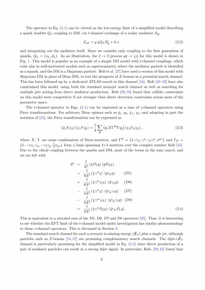
The operator in Eq. (2.1) can be viewed as the low-energy limit of a simplified model describing
a quark doublet QL coupling to DM, via t-channel exchange of a scalar mediator SQ,
Lint = g χQLS∗Q + h.c. (2.2)
and integrating out the mediator itself. Since we consider only coupling to the first generation of
quarks, QL = (uL, dL). As an illustration, the 2 → 2 process qq → χχ for this model is shown in
Fig. 1. This model is popular as an example of a simple DM model with t-channel couplings, which
exist also in well-motivated models such as supersymmetry where the mediator particle is identified
as a squark, and the DM is a Majorana particle. Bell et al. [27] have used a version of this model with
Majorana DM in place of Dirac DM, to test the prospects of Z-bosons as a potential search channel.
This has been followed up by a dedicated ATLAS search in this channel [16]. Refs [28–33] have also
constrained this model, using both the standard monojet search channel as well as searching for
multiple jets arising from direct mediator production. Refs [29, 33] found that collider constraints
on this model were competitive if not stronger than direct detection constraints across most of the
parameter space.
The t-channel operator in Eqn. (2.1) can be expressed as a sum of s-channel operators using
Fierz transformations. For arbitrary Dirac spinors such as q1, q2, χ1, χ2, and adopting in part the
notation of [34], the Fierz transformation can be expressed as
(q1Xχ2) (χ1Y q2) =1
4
∑B
(q1XΓBY q2
)(χ1ΓBχ2) , (2.3)
where X, Y are some combination of Dirac-matrices, and ΓB = 1, iγ5, γµ, γ5γ
µ, σµν and ΓB =
1,−iγ5, γµ,−γ5γµ,12σµν form a basis spanning 4×4 matrices over the complex number field [34].
Due to the chiral coupling between the quarks and DM, most of the terms in the sum cancel, and
we are left with
O =1
Λ2(χPLq) (qPRχ)
=1
8Λ2(χγµχ) (qγµq) (D5)
+1
8Λ2(χγµγ5χ) (qγµq) (D6)
− 1
8Λ2(χγµχ) (qγµγ5q) (D7)
− 1
8Λ2(χγµγ5χ) (qγµγ5q) (D8)
=1
2Λ2(χγµPRχ) (qγµPLq) . (2.4)
This is equivalent to a rescaled sum of the D5, D6, D7 and D8 operators [35]. Thus, it is interesting
to see whether the EFT limit of the t-channel model under investigation has similar phenomenology
to these s-channel operators. This is discussed in Section 3.
The standard search channel for such a scenario is missing energy (/ET ) plus a single jet, although
particles such as Z-bosons [16, 27] are promising complementary search channels. The dijet+/ETchannel is particularly promising for the simplified model in Eq. (2.2) since direct production of a
pair of mediator particles can result in a strong dijet signal. In particular, Refs. [29, 32] found that
3
S
q
q
Figure 1: Illustrative 2→ 2 process for the UV-complete version of our effective operator.
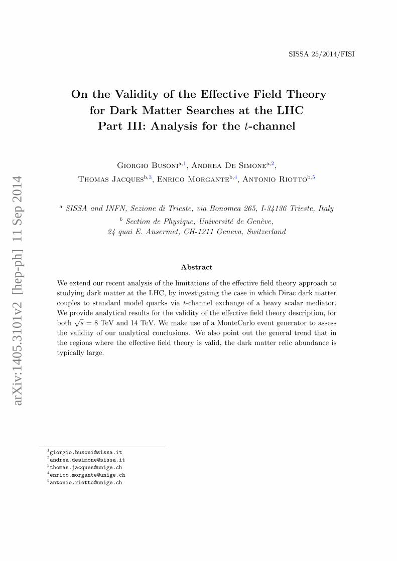
q
q
jet
q
q
jet
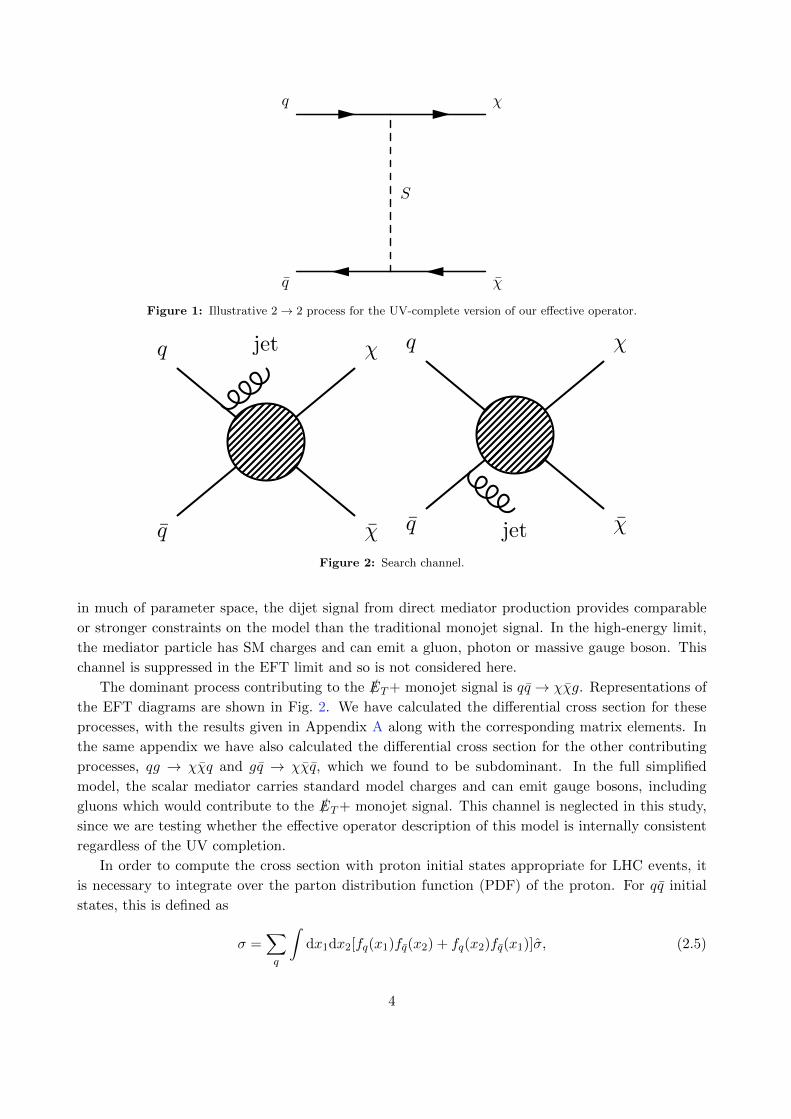
Figure 2: Search channel.
in much of parameter space, the dijet signal from direct mediator production provides comparable
or stronger constraints on the model than the traditional monojet signal. In the high-energy limit,
the mediator particle has SM charges and can emit a gluon, photon or massive gauge boson. This
channel is suppressed in the EFT limit and so is not considered here.
The dominant process contributing to the /ET+ monojet signal is qq → χχg. Representations of
the EFT diagrams are shown in Fig. 2. We have calculated the differential cross section for these
processes, with the results given in Appendix A along with the corresponding matrix elements. In
the same appendix we have also calculated the differential cross section for the other contributing
processes, qg → χχq and gq → χχq, which we found to be subdominant. In the full simplified
model, the scalar mediator carries standard model charges and can emit gauge bosons, including
gluons which would contribute to the /ET+ monojet signal. This channel is neglected in this study,
since we are testing whether the effective operator description of this model is internally consistent
regardless of the UV completion.
In order to compute the cross section with proton initial states appropriate for LHC events, it
is necessary to integrate over the parton distribution function (PDF) of the proton. For qq initial
states, this is defined as
σ =∑q
∫dx1dx2[fq(x1)fq(x2) + fq(x2)fq(x1)]σ, (2.5)
4
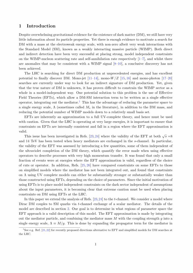
mDM=10GeV
mDM=500GeV
mDM=1000GeV
s = 8TeV
500GeV £ pT £ 1 TeV, Η £ 2
1 2 3 4 50.0
0.2
0.4
0.6
0.8
1.0
L @TeVD
RL
mDM=10GeV
mDM=1000GeV
mDM=2000GeV
s =14TeV
500GeV £ pT £ 2 TeV, Η £ 2
1 2 3 4 5 6 7 80.0
0.2
0.4
0.6
0.8
1.0
L @TeVD
RL
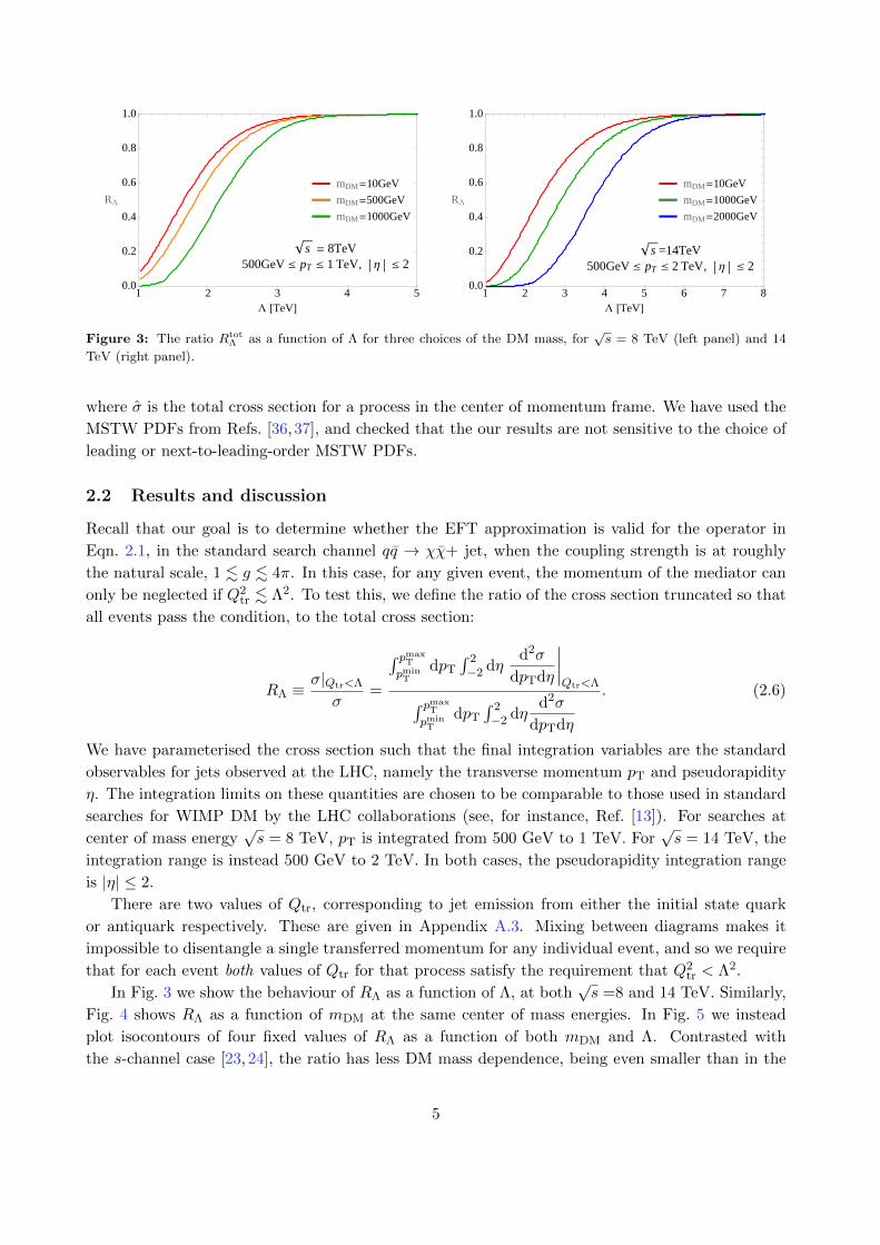
Figure 3: The ratio RtotΛ as a function of Λ for three choices of the DM mass, for
√s = 8 TeV (left panel) and 14
TeV (right panel).
where σ is the total cross section for a process in the center of momentum frame. We have used the
MSTW PDFs from Refs. [36,37], and checked that the our results are not sensitive to the choice of
leading or next-to-leading-order MSTW PDFs.
2.2 Results and discussion
Recall that our goal is to determine whether the EFT approximation is valid for the operator in
Eqn. 2.1, in the standard search channel qq → χχ+ jet, when the coupling strength is at roughly
the natural scale, 1 . g . 4π. In this case, for any given event, the momentum of the mediator can
only be neglected if Q2tr . Λ2. To test this, we define the ratio of the cross section truncated so that
all events pass the condition, to the total cross section:
RΛ ≡σ|Qtr<Λ
σ=
∫ pmaxT
pminT
dpT
∫ 2−2 dη
d2σ
dpTdη
∣∣∣∣Qtr<Λ∫ pmax
T
pminT
dpT
∫ 2−2 dη
d2σ
dpTdη
. (2.6)
We have parameterised the cross section such that the final integration variables are the standard
observables for jets observed at the LHC, namely the transverse momentum pT and pseudorapidity
η. The integration limits on these quantities are chosen to be comparable to those used in standard
searches for WIMP DM by the LHC collaborations (see, for instance, Ref. [13]). For searches at
center of mass energy√s = 8 TeV, pT is integrated from 500 GeV to 1 TeV. For
√s = 14 TeV, the
integration range is instead 500 GeV to 2 TeV. In both cases, the pseudorapidity integration range
is |η| ≤ 2.
There are two values of Qtr, corresponding to jet emission from either the initial state quark
or antiquark respectively. These are given in Appendix A.3. Mixing between diagrams makes it
impossible to disentangle a single transferred momentum for any individual event, and so we require
that for each event both values of Qtr for that process satisfy the requirement that Q2tr < Λ2.
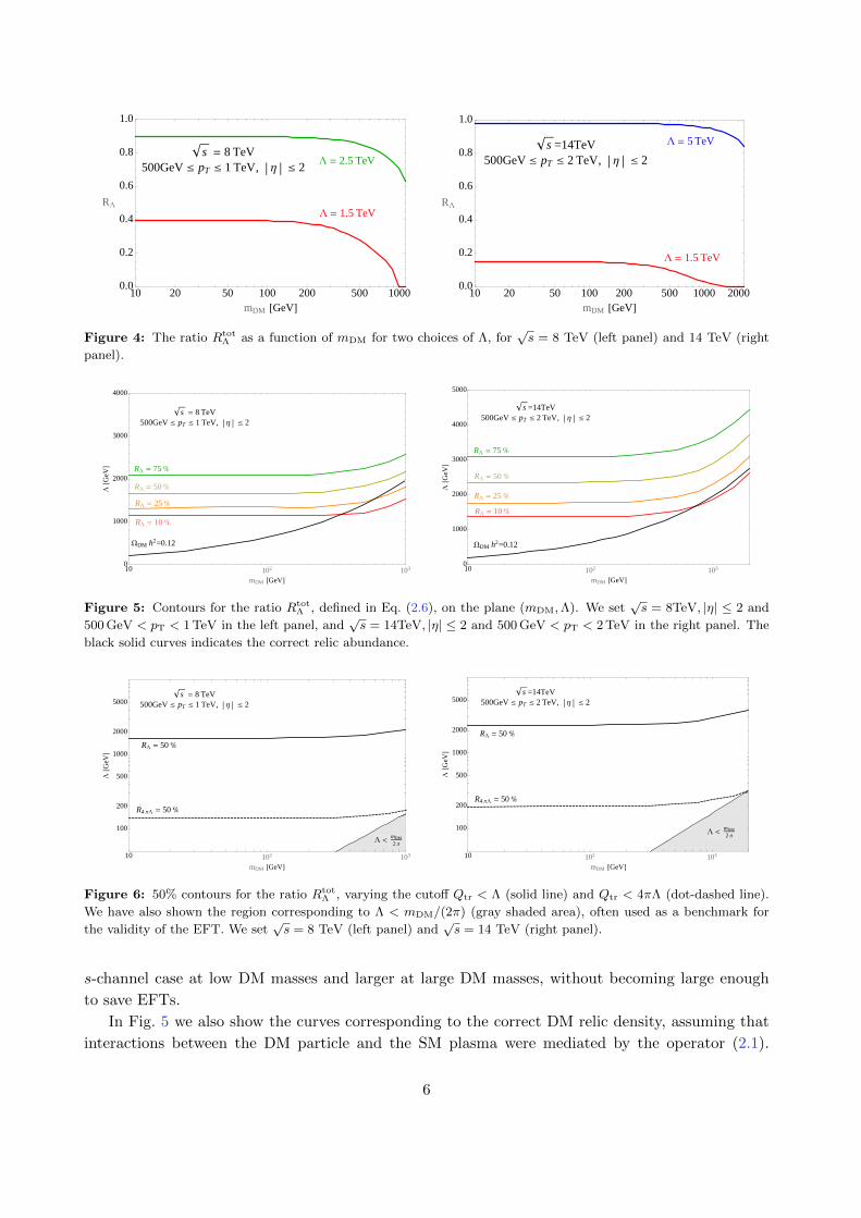
In Fig. 3 we show the behaviour of RΛ as a function of Λ, at both√s =8 and 14 TeV. Similarly,
Fig. 4 shows RΛ as a function of mDM at the same center of mass energies. In Fig. 5 we instead
plot isocontours of four fixed values of RΛ as a function of both mDM and Λ. Contrasted with
the s-channel case [23, 24], the ratio has less DM mass dependence, being even smaller than in the
5
s = 8 TeV
500GeV £ pT £ 1 TeV, Η £ 2L = 2.5 TeV
L = 1.5 TeV
10 20 50 100 200 500 10000.0
0.2
0.4
0.6
0.8
1.0
mDM @GeVD
RL
L = 5 TeVs =14TeV
500GeV £ pT £ 2 TeV, Η £ 2
L = 1.5 TeV
10 20 50 100 200 500 1000 20000.0
0.2
0.4
0.6
0.8
1.0
mDM @GeVD
RL
Figure 4: The ratio RtotΛ as a function of mDM for two choices of Λ, for
√s = 8 TeV (left panel) and 14 TeV (right
panel).
s = 8 TeV
500GeV £ pT £ 1 TeV, Η £ 2
RL = 75 %
RL = 50 %
RL = 25 %
RL = 10 %
WDM h2=0.12
10 102 1030
1000
2000
3000
4000
mDM @GeVD
L@G
eVD
s =14TeV
500GeV £ pT £ 2 TeV, Η £ 2
RL = 75 %
RL = 50 %
RL = 25 %
RL = 10 %
WDM h2=0.12
10 102 1030
1000
2000
3000
4000
5000
mDM @GeVD
L@G
eVD
Figure 5: Contours for the ratio RtotΛ , defined in Eq. (2.6), on the plane (mDM,Λ). We set
√s = 8TeV, |η| ≤ 2 and
500 GeV < pT < 1 TeV in the left panel, and√s = 14TeV, |η| ≤ 2 and 500 GeV < pT < 2 TeV in the right panel. The
black solid curves indicates the correct relic abundance.
s = 8 TeV
500GeV £ pT £ 1 TeV, Η £ 2
RL = 50 %
R4 ΠL = 50 %
L < mDM
2 Π
10 102 103
100
200
500
1000
2000
5000
mDM @GeVD
L@G
eVD
s =14TeV
500GeV £ pT £ 2 TeV, Η £ 2
RL = 50 %
R4 ΠL = 50 %
L < mDM
2 Π
10 102 103
100
200
500
1000
2000
5000
mDM @GeVD
L@G
eVD
Figure 6: 50% contours for the ratio RtotΛ , varying the cutoff Qtr < Λ (solid line) and Qtr < 4πΛ (dot-dashed line).
We have also shown the region corresponding to Λ < mDM/(2π) (gray shaded area), often used as a benchmark for
the validity of the EFT. We set√s = 8 TeV (left panel) and
√s = 14 TeV (right panel).
s-channel case at low DM masses and larger at large DM masses, without becoming large enough
to save EFTs.
In Fig. 5 we also show the curves corresponding to the correct DM relic density, assuming that
interactions between the DM particle and the SM plasma were mediated by the operator (2.1).
6
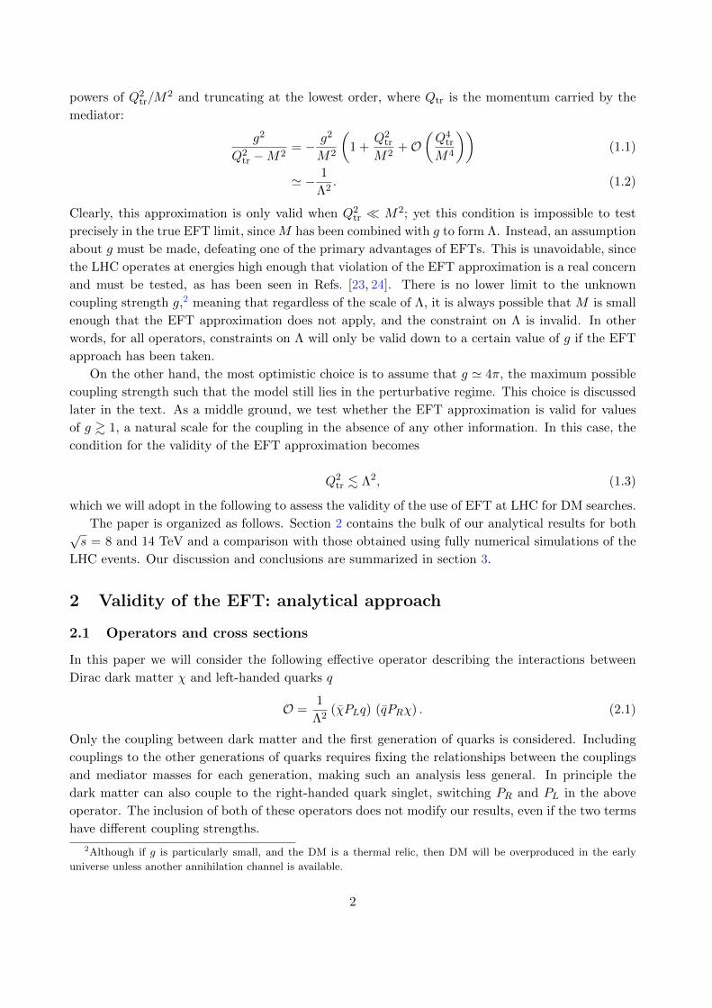
=
≤ ≤ η ≤
Λ=
-
-
-
[]
σ[]
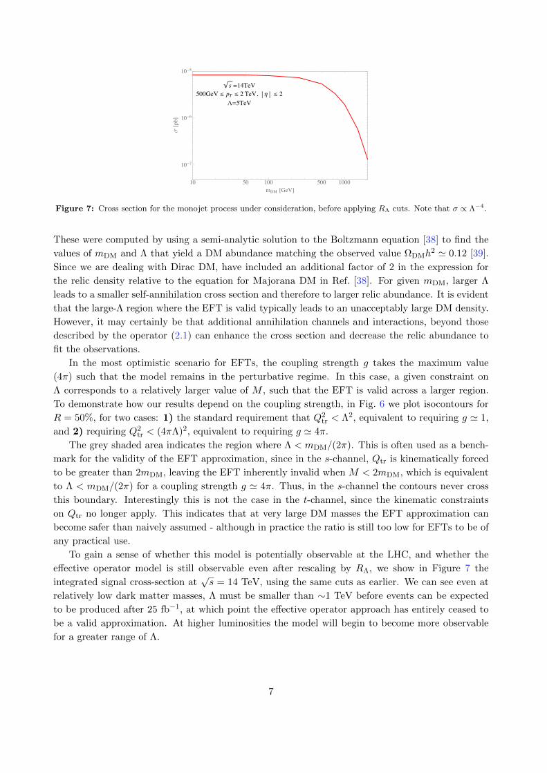
Figure 7: Cross section for the monojet process under consideration, before applying RΛ cuts. Note that σ ∝ Λ−4.
These were computed by using a semi-analytic solution to the Boltzmann equation [38] to find the
values of mDM and Λ that yield a DM abundance matching the observed value ΩDMh2 ' 0.12 [39].
Since we are dealing with Dirac DM, have included an additional factor of 2 in the expression for
the relic density relative to the equation for Majorana DM in Ref. [38]. For given mDM, larger Λ
leads to a smaller self-annihilation cross section and therefore to larger relic abundance. It is evident
that the large-Λ region where the EFT is valid typically leads to an unacceptably large DM density.
However, it may certainly be that additional annihilation channels and interactions, beyond those
described by the operator (2.1) can enhance the cross section and decrease the relic abundance to
fit the observations.
In the most optimistic scenario for EFTs, the coupling strength g takes the maximum value
(4π) such that the model remains in the perturbative regime. In this case, a given constraint on
Λ corresponds to a relatively larger value of M , such that the EFT is valid across a larger region.
To demonstrate how our results depend on the coupling strength, in Fig. 6 we plot isocontours for
R = 50%, for two cases: 1) the standard requirement that Q2tr < Λ2, equivalent to requiring g ' 1,
and 2) requiring Q2tr < (4πΛ)2, equivalent to requiring g ' 4π.
The grey shaded area indicates the region where Λ < mDM/(2π). This is often used as a bench-
mark for the validity of the EFT approximation, since in the s-channel, Qtr is kinematically forced
to be greater than 2mDM, leaving the EFT inherently invalid when M < 2mDM, which is equivalent
to Λ < mDM/(2π) for a coupling strength g ' 4π. Thus, in the s-channel the contours never cross
this boundary. Interestingly this is not the case in the t-channel, since the kinematic constraints
on Qtr no longer apply. This indicates that at very large DM masses the EFT approximation can
become safer than naively assumed - although in practice the ratio is still too low for EFTs to be of
any practical use.
To gain a sense of whether this model is potentially observable at the LHC, and whether the
effective operator model is still observable even after rescaling by RΛ, we show in Figure 7 the
integrated signal cross-section at√s = 14 TeV, using the same cuts as earlier. We can see even at
relatively low dark matter masses, Λ must be smaller than ∼1 TeV before events can be expected
to be produced after 25 fb−1, at which point the effective operator approach has entirely ceased to
be a valid approximation. At higher luminosities the model will begin to become more observable
for a greater range of Λ.
7
s =14TeV
500GeV £ pT £ 2 TeV, Η £ 2
RL = 75 %
RL = 50 %
RL = 25 %
RL = 10 %
Calculation
Simulation
WDM h2=0.12
10 102 1030
1000
2000
3000
4000
5000
mDM @GeVD
L@G
eVD
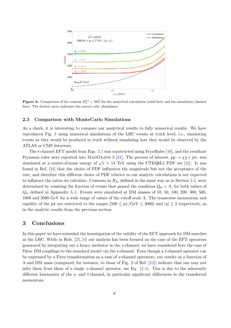
Figure 8: Comparison of the contour RtotΛ = 50% for the analytical calculation (solid line) and the simulation (dashed
line). The dotted curve indicates the correct relic abundance.
2.3 Comparison with MonteCarlo Simulations
As a check, it is interesting to compare our analytical results to fully numerical results. We have
reproduced Fig. 3 using numerical simulations of the LHC events at truth level, i.e., simulating
events as they would be produced in truth without simulating how they would be observed by the
ATLAS or CMS detectors.
The t-channel EFT model from Eqn. 2.1 was constructed using FeynRules [40], and the resultant
Feynman rules were exported into MadGraph 5 [41]. The process of interest, pp → χχ+ jet, was
simulated at a center-of-mass energy of√s = 14 TeV using the CTEQ6L1 PDF set [42]. It was
found in Ref. [24] that the choice of PDF influences the magnitude but not the acceptance of the
rate, and therefore this different choice of PDF relative to our analytic calculations is not expected
to influence the ratios we calculate. Contours in RΛ, defined in the same way as in Section 2.2, were
determined by counting the fraction of events that passed the condition Qtr < Λ, for both values of
Qtr defined in Appendix A.3. Events were simulated at DM masses of 10, 50, 100, 200, 300, 500,
1000 and 2000 GeV for a wide range of values of the cutoff scale Λ. The transverse momentum and
rapidity of the jet are restricted to the ranges (500 ≤ pT/GeV ≤ 2000) and |η| ≤ 2 respectively, as
in the analytic results from the previous section.
3 Conclusions
In this paper we have extended the investigation of the validity of the EFT approach for DM searches
at the LHC. While in Refs. [23, 24] our analysis has been focused on the case of the EFT operators
generated by integrating out a heavy mediator in the s-channel, we have considered here the case of
Dirac DM couplings to the standard model via the t-channel. Even though a t-channel operator can
be expressed by a Fierz transformation as a sum of s-channel operators, our results as a function of
Λ and DM mass (compared, for instance, to those of Fig. 2 of Ref. [24]) indicate that one may not
infer them from those of a single s-channel operator, see Eq. (2.4). This is due to the inherently
different kinematics of the s- and t-channel, in particular significant differences in the transferred
momentum.
8
We have also computed the relic density over the parameter space of the model, assuming that the
only interactions between DM and the SM are those mediated by the t-channel operator (2.1), and
found that the region of EFT validity corresponds to an overly large relic density. This conclusion
is rather general and may be evaded by assuming additional DM annihilation channels.
Similar to what happens in the s-channel case, our findings indicate that in the t-channel the
range of validity of the EFT is significantly limited in the parameter space (Λ,mDM), reinforcing
the need to go beyond the EFT at the LHC when looking for DM signals. This is especially true
for light mediators as they can be singly produced in association with a DM particle, leading to
a qualitatively new contribution to the mono-jet processes. Mediators can even be pair-produced
at the LHC through both QCD processes and DM exchange processes. All of this rich dynamics
leads to stronger signals (and therefore, in the absence thereof, to tighter bounds) than the EFT
approach.
Acknowledgments
We thank A. Brennan, C. Doglioni, G. Iacobucci, S. Schramm and S. Vallecorsa for many interesting
conversations. ADS acknowledges partial support from the European Union FP7 ITN INVISIBLES
(Marie Curie Actions, PITN-GA-2011-289442).
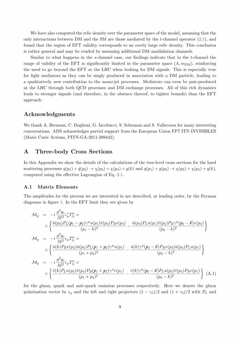
A Three-body Cross Sections
In this Appendix we show the details of the calculations of the tree-level cross sections for the hard
scattering processes q(p1) + q(p2)→ χ(p3) + χ(p4) + g(k) and q(p1) + g(p2)→ χ(p3) + χ(p4) + q(k),
computed using the effective Lagrangian of Eq. 2.1.
A.1 Matrix Elements
The amplitudes for the process we are interested in are described, at leading order, by the Feyman
diagrams in figure 1. In the EFT limit they are given by
Mg = −i g2gsM2
ε∗µTaij ×
×u(p3)PL(p1 − p2)γµu(p1)v(p2)PRv(p4)
(p1 − k)2− u(p3)PLu(p1)v(p2)PRγ
µ(p2 −k)v(p4)
(p2 − k)2
Mq = −i g
2gsM2
εµTaij ×
×u(k)PRv(p3)u(p4)PL(p1 + p2)γµu(p1)
(p1 + p2)2− u(k)γµ(p2 −k)PRv(p3)u(p4)PLu(p1)
(p2 − k)2
Mq = −i g
2gsM2
εµTaij ×
×v(k)PLu(p3)v(p4)PR(p1 + p2)γµv(p1)
(p1 + p2)2− v(k)γµ(p2 −k)PLu(p3)v(p4)PRv(p1)
(p2 − k)2
(A.1)
for the gluon, quark and anti-quark emission processes respectively. Here we denote the gluon
polarization vector by εµ and the left and right projectors (1 − γ5)/2 and (1 + γ5)/2 with PL and
9
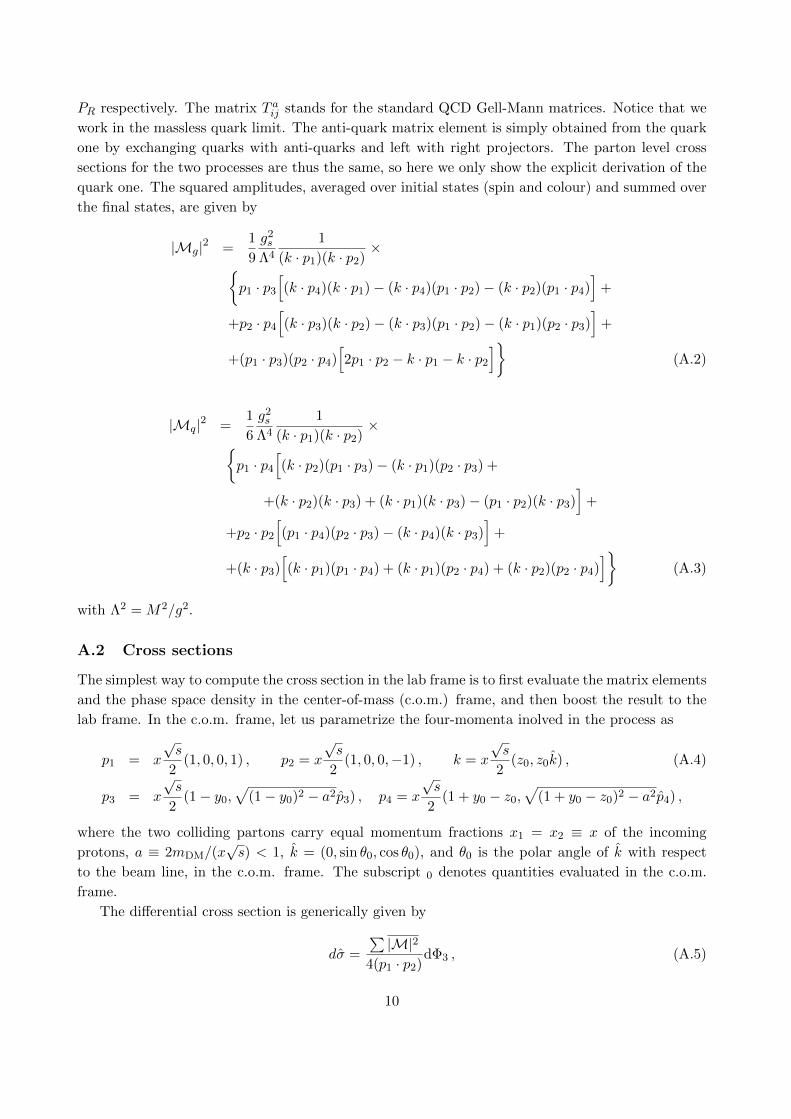
PR respectively. The matrix T aij stands for the standard QCD Gell-Mann matrices. Notice that we
work in the massless quark limit. The anti-quark matrix element is simply obtained from the quark
one by exchanging quarks with anti-quarks and left with right projectors. The parton level cross
sections for the two processes are thus the same, so here we only show the explicit derivation of the
quark one. The squared amplitudes, averaged over initial states (spin and colour) and summed over
the final states, are given by
|Mg|2 =1
9
g2s
Λ4
1
(k · p1)(k · p2)×
p1 · p3
[(k · p4)(k · p1)− (k · p4)(p1 · p2)− (k · p2)(p1 · p4)
]+
+p2 · p4
[(k · p3)(k · p2)− (k · p3)(p1 · p2)− (k · p1)(p2 · p3)
]+
+(p1 · p3)(p2 · p4)[2p1 · p2 − k · p1 − k · p2
](A.2)
|Mq|2 =1
6
g2s
Λ4
1
(k · p1)(k · p2)×
p1 · p4
[(k · p2)(p1 · p3)− (k · p1)(p2 · p3) +
+(k · p2)(k · p3) + (k · p1)(k · p3)− (p1 · p2)(k · p3)]
+
+p2 · p2
[(p1 · p4)(p2 · p3)− (k · p4)(k · p3)
]+
+(k · p3)[(k · p1)(p1 · p4) + (k · p1)(p2 · p4) + (k · p2)(p2 · p4)
](A.3)
with Λ2 = M2/g2.
A.2 Cross sections
The simplest way to compute the cross section in the lab frame is to first evaluate the matrix elements
and the phase space density in the center-of-mass (c.o.m.) frame, and then boost the result to the
lab frame. In the c.o.m. frame, let us parametrize the four-momenta inolved in the process as
p1 = x
√s
2(1, 0, 0, 1) , p2 = x
√s
2(1, 0, 0,−1) , k = x
√s
2(z0, z0k) , (A.4)
p3 = x
√s
2(1− y0,
√(1− y0)2 − a2p3) , p4 = x
√s
2(1 + y0 − z0,
√(1 + y0 − z0)2 − a2p4) ,
where the two colliding partons carry equal momentum fractions x1 = x2 ≡ x of the incoming
protons, a ≡ 2mDM/(x√s) < 1, k = (0, sin θ0, cos θ0), and θ0 is the polar angle of k with respect
to the beam line, in the c.o.m. frame. The subscript 0 denotes quantities evaluated in the c.o.m.
frame.
The differential cross section is generically given by
dσ =
∑|M|2
4(p1 · p2)dΦ3 , (A.5)
10
where the three-body phase space is
dΦ3 = (2π)4 δ(E1 +E2−E3−E4−Ek) δ(3)(~p1 +~p2−~p3−~p4−~k)d3p3
(2π)32E3
d3p4
(2π)32E4
d3k
(2π)32Ek. (A.6)
Using the three-momentum delta function, we can integrate away d3p4; the energy delta function
instead fixes the angle θ0 3j between p3 and the jet k as: cos θ0 3j = (p24−k2−p2
3)/2|k||p3|. Integration
over the azimuthal angle φ0 of the outgoing jet simply gives a factor of 2π, while the matrix element
does depend on the azimuthal angle of the three-momentum ~p3 with respect to ~k, φ0 3j, and so it can
not be integrated over at this stage, contrary to the s-channel case. Taking all of this into account,
the phase space density simplifies to
dΦ3 =1
8(2π)4dE3 d|~k| d cos θ0 dφ0 3j =
x2s
32(2π)4dy0 dz0 d cos θ0 dφ0 3j. (A.7)
The kinematical domains of y0, z0 and φ0 3j are
z0
2
1−
√1− z0 − a2
1− z0
≤ y0 ≤ z0
2
1 +
√1− z0 − a2
1− z0
(A.8)
0 ≤ z0 ≤ 1− a2 (A.9)
0 ≤ φ0 3j ≤ 2π (A.10)
The variables y0 and φ0 3j refer to the momentum ~p3 of an invisible DM particle; they are therefore
not measurable, and we integrate over them. For our present purpose, finding the total integrated
cross section is useless, since these variables enter our definition of the momentum transfer Qtr, and
the condition Qtr < Λ which we used to define the ratio RΛ.
With the matrix elements of Eqns. A.2 and A.3, and the phase space density A.7, we get the
differential cross sections in the c.o.m. frame:
d4σ
dz0 d cos θ0 dy0 dφ0 3j
∣∣∣∣g
=1
4608π4
g2s
Λ4
1− z0
z40
4x(2− z0) csc θ0 cosφ0 3j(cos θ0(z0 − 2y0) + z0)√s(sx2y0(z0 − 1)(y0 − z0)−m2
DMz20
)−8m2
DMz20 cos2 φ0 3j + sx2((z0 − 2)z0 + 2)
(sec2 (θ0/2) y2
0 + csc2 (θ0/2) (y0 − z0)2)
−2sx2y20((z0 − 6)z0 + 6) + 4sx2y0(z0 − 1)(y0 − z0) cos(2φ0 3j)
+2sx2y0((z0 − 6)z0 + 6)z0 − sx2z20((z0 − 2)z0 + 2)
, (A.11)
11
d4σ
dz0 d cos θ0 dy0 dφ0 3j
∣∣∣∣q
=1
98304π4
g2s
Λ4
1− z0
z30 cos2 θ0
28x√s[z0(z0 − y0 − 1)−
(z2
0 − (1 + y0)z0 + 2y0
)cos θ0
]cosφ0 3j sin θ0 ×
×√sx2y0(z0 − y0)(1− z0)−m2
DMz20
−2(1− cos(2θ0))m2DMz
20 + 4
[sx2y0(z0 − y0)(1− z0)−m2
DMz20
]cos(2φ0 3j) sin2 θ0
+sx2[11z4
0 − (6 + 22y0)z30 + (11y2
0 + 8y0 + 3)z20 − 2y0(1 + y0)z0 + 2y2
0
]+sx2
[z4
0 − 2(1 + y0)z30 + (y2
0 + 8y0 + 1)z20 − 6y0(1 + y0)z0 + 6y2
0
]cos(2θ0)
−4sx2z0
[z3
0 − 2(1 + y0)z20 + (y2
0 + 4y0 + 1)z0 − 2y0(1 + y0)]
cos θ0
.
(A.12)
To get the cross sections in the lab frame we perform a boost in the z axis, accounting for the
generic parton momentum fractions x1, x2. The velocity of the c.o.m. of the colliding particles with
respect to the lab frame is given by
βc.o.m. =x1 − x2
x1 + x2, (A.13)
so that the relations between the quantities z0, θ0 and the analogous ones z, θ in the lab frame are
z0 =(x1 + x2)2 + (x2
2 − x21) cos θ
4x1x2z
sin2 θ0 =4x1x2
[(x1 + x2) + (x2 − x1) cos θ]2sin2 θ. (A.14)
The Jacobian factor to transform dz0 d cos θ0 → dz d cos θ is simply obtained using equations A.14;
the cross section in the lab frame is then
d4σ
dz d cos θ dy0 dφ0 3j=
x1 + x2
x1 + x2 + (x1 − x2) cos θ
d4σ
dz0 d cos θ0 dy0 dφ0 3j
∣∣∣∣ z0 → z0(z)
θ0 → θ0(θ)
. (A.15)
Expressing the energy of the emitted gluon or (anti-)quark in terms of the transverse momentum
and rapidity, k0 = pT cosh η, one finds
z =4pT cosh η
(x1 + x2)√s, cos θ = tanh η (A.16)
which allows us to express the differential cross sections with respect to the transverse momentum
and pseudo-rapidity of the emitted jet:
d4σ
dpT dη dy0 dφ0 3j=
4
(x1 + x2)√s cosh η
d4σ
dz d cos θ dy0 dφ0 3j
∣∣∣∣ z → z(pT, η)
θ → θ(pT, η)
. (A.17)
12
A.3 Transferred momentum
As is clear from our arguments, the key ingredient to quantify the validity of the EFT approximation
is the value of the transferred momentum of the process. Since each process of interest here is given
(at tree level) by the contribution of two Feynman diagrams, there will also be two expressions for
the transferred momentum for both gluon and (anti-)quark emission, which we report here:
Q2tr,g1 = (p1 − k − p3)2
= m2DM +
√sx2e
ηpT −e2η(1 + y)(x1x
22s)
x1 + e2ηx2−x2
1x22eηs3/2y
(x1 − e2ηx2
)pT(x1 + e2ηx2)2
−2eηx1x2√s cosφ0 3j
pT(x1 + e2ηx2)2
[−m2
DMp2T
(x1 + e2ηx2
)2(A.18)
−sx1x2y(eη√sx1x2 − pT
(x1 + e2ηx2
)) (eη√sx1x2y − pT
(x1 + e2ηx2
))]1/2,
Q2tr,g2 = (p1 − p3)2
= m2DM +
x1x2s(x1 − e2ηx2)
x1 + e2ηx2− (1− y)(x2
1x2s)
x1 + e2ηx2− x2
1x22eηs3/2y(x1 − e2ηx2)
pT(x1 + e2ηx2)2
−2eηx1x2√s cosφ0 3j
pT(x1 + e2ηx2)2
[−m2
DMp2T
(x1 + e2ηx2
)2(A.19)
−sx1x2y(eη√sx1x2 − pT
(x1 + e2ηx2
)) (eη√sx1x2y − pT
(x1 + e2ηx2
))]1/2,
Q2tr,q1 = (p3 + k)2
= m2DM + pT
√s(e−ηx1 + eηx2
)− x1x2s y, (A.20)
Q2tr,q2 = (p1 − p3 − k)2
= m2DM +
√sx1e
−ηpT −(1 + y)(x2
1x2s)
x1 + e2ηx2+x2
1x22eηs3/2y(x1 − e2ηx2)
pT(x1 + e2ηx2)2
−2eηx1x2√s cosφ0 3j
pT(x1 + e2ηx2)2
[−m2
DMp2T
(x1 + e2ηx2
)2(A.21)
−sx1x2y(eη√sx1x2 − pT
(x1 + e2ηx2
)) (eη√sx1x2y − pT
(x1 + e2ηx2
))]1/2.
The notation g, q stands for gluon or quark emission; the indices 1, 2 refer to emission from each of
the initial state particles.
References
[1] L. Baudis, Phys.Dark Univ. 1, 94 (2012), arXiv:1211.7222.
[2] M. Cirelli, Pramana 79, 1021 (2012), arXiv:1202.1454.
[3] J. Feng et al., (2014), arXiv:1401.6085.
13
[4] H.E.S.S.Collaboration, A. Abramowski et al., Phys.Rev.Lett. 106, 161301 (2011),
arXiv:1103.3266.
[5] Fermi-LAT Collaboration, M. Ackermann et al., Phys.Rev. D89, 042001 (2014),
arXiv:1310.0828.
[6] XENON100 Collaboration, E. Aprile et al., Phys.Rev.Lett. 109, 181301 (2012),
arXiv:1207.5988.
[7] LUX Collaboration, D. Akerib et al., (2013), arXiv:1310.8214.
[8] DAMA Collaboration, LIBRA Collaboration, R. Bernabei et al., Eur.Phys.J. C67, 39 (2010),
arXiv:1002.1028.
[9] CDMS Collaboration, R. Agnese et al., Phys.Rev.Lett. 111, 251301 (2013), arXiv:1304.4279.
[10] CoGeNT Collaboration, C. Aalseth et al., Phys.Rev. D88, 012002 (2013), arXiv:1208.5737.
[11] ATLAS Collaboration, G. Aad et al., JHEP 1304, 075 (2013), arXiv:1210.4491.
[12] CMS Collaboration, S. Chatrchyan et al., Phys.Rev.Lett. 107, 201804 (2011), arXiv:1106.4775.
[13] ATLAS Collaboration, (2012).
[14] CMS Collaboration, (2013).
[15] T. A. collaboration, (2013).
[16] ATLAS Collaboration, G. Aad et al., (2014), arXiv:1404.0051.
[17] ATLAS Collaboration, G. Aad et al., Phys.Rev.Lett. 110, 011802 (2013), arXiv:1209.4625.
[18] CMS Collaboration, S. Chatrchyan et al., Phys.Rev.Lett. 108, 261803 (2012), arXiv:1204.0821.
[19] ATLAS Collaboration, (2012).
[20] CMS Collaboration, C. Collaboration, (2011).
[21] A. De Simone, G. F. Giudice, and A. Strumia, (2014), arXiv:1402.6287.
[22] A. Alves, S. Profumo, and F. S. Queiroz, JHEP 1404, 063 (2014), arXiv:1312.5281.
[23] G. Busoni, A. De Simone, E. Morgante, and A. Riotto, Phys.Lett. B728, 412 (2014),
arXiv:1307.2253.
[24] G. Busoni, A. De Simone, J. Gramling, E. Morgante, and A. Riotto, (2014), arXiv:1402.1275.
[25] P. J. Fox, R. Harnik, J. Kopp, and Y. Tsai, Phys.Rev. D85, 056011 (2012), arXiv:1109.4398.
[26] O. Buchmueller, M. J. Dolan, and C. McCabe, JHEP 1401, 025 (2014), arXiv:1308.6799.
[27] N. F. Bell et al., Phys.Rev. D86, 096011 (2012), arXiv:1209.0231.
14
[28] S. Chang, R. Edezhath, J. Hutchinson, and M. Luty, Phys.Rev. D89, 015011 (2014),
arXiv:1307.8120.
[29] H. An, L.-T. Wang, and H. Zhang, (2013), arXiv:1308.0592.
[30] Y. Bai and J. Berger, JHEP 1311, 171 (2013), arXiv:1308.0612.
[31] A. DiFranzo, K. I. Nagao, A. Rajaraman, and T. M. P. Tait, JHEP 1311, 014 (2013),
arXiv:1308.2679.
[32] M. Papucci, A. Vichi, and K. M. Zurek, (2014), arXiv:1402.2285.
[33] M. Garny, A. Ibarra, S. Rydbeck, and S. Vogl, (2014), arXiv:1403.4634.
[34] N. F. Bell, J. B. Dent, T. D. Jacques, and T. J. Weiler, Phys.Rev. D83, 013001 (2011),
arXiv:1009.2584.
[35] J. Goodman et al., Phys.Rev. D82, 116010 (2010), arXiv:1008.1783.
[36] A. Martin, W. Stirling, R. Thorne, and G. Watt, Eur.Phys.J. C63, 189 (2009), arXiv:0901.0002.
[37] http://mstwpdf.hepforge.org/ .
[38] G. Bertone, D. Hooper, and J. Silk, Phys.Rept. 405, 279 (2005), arXiv:hep-ph/0404175.
[39] Planck Collaboration, P. Ade et al., (2013), arXiv:1303.5076.
[40] N. D. Christensen and C. Duhr, Comput.Phys.Commun. 180, 1614 (2009), arXiv:0806.4194.
[41] J. Alwall, M. Herquet, F. Maltoni, O. Mattelaer, and T. Stelzer, JHEP 1106, 128 (2011),
arXiv:1106.0522.
[42] J. Pumplin et al., JHEP 0207, 012 (2002), arXiv:hep-ph/0201195.
15
Recommended