hep-th/9802162 SLAC-PUB-7751
UCLA/98/TEP/03 SWAT-98-183
February, 1998
On the Relationship between Yang-Mills Theory and Gravity and its Implication for Ultraviolet Divergences
Z. Bern*>‘, L. Dixontf2, D.C. Dunbarflr3, M. Perelsteintf2 and J.S. Rozowsky**’
*Department of Physics, University of California at Los Angeles, Los Angeles, CA 90095-1547
+Stanford Linear Accelerator Center, Stanford University, Stanford, CA 94309
UDepartment of Physics, University of Wales Swansea, Swansea, SA2 8PP, UK
Abstract
String theory implies that field theories containing gravity are in a certain sense ‘products’ of
gauge theories. We make this product structure explicit up to two loops for the relatively simple case of N = 8 supergravity four-point amplitudes, demonstrating that they are ‘squares’ of N = 4 super-Yang-Mills amplitudes. This is accomplished by obtaining an explicit expression for the
D-dimensional two-loop contribution to the four-particle S-matrix for N = 8 supergravity, which we compare to the corresponding N = 4 Yang-Mills result. F’rom these expressions we also obtain the two-loop ultraviolet divergences in D = 7,9,11. The analysis relies on the unitarity cuts of the two theories, many of which can be recycled from a one-loop computation. The two-particle cuts, which may be iterated to all loop orders, suggest that squaring relations between the two theories exist at any loop order. The loop-momentum power-counting implied by our two-particle cut analysis indicates that in four dimensions the first four-point divergence in N = 8 supergravity should appear at five loops, contrary to the earlier expectation, based on superspace arguments, of a three-loop counterterm.
Submitted to Nuclear Physics B
‘Research supported in part by the US Department of Energy under grant DE-FG03-91ER40662
2Research supported by the US Department of Energy under grant DE-AC03-76SF00515.
3Research supp orted in part by the Leverhulme Foundation.

1 Introduction
Gravity and gauge theories both contain a local symmetry, mediate long-range forces at the classical
level, and have a number of other well-known similarities. Indeed, one might naively suspect that
a spin two graviton can in some way be interpreted as a product of spin one gluons. There are,
however, some important differences. In particular, the Feynman rules for gauge field perturbation
theory include only three- and four-point vertices, while those for gravity can have arbitrarily many
external legs. A related fact is that gauge theories are renormalizable in four dimensions, while
gravity is not. Given the rather disparate forms of the Yang-Mills and Einstein-Hilbert Lagrangians,
it is not obvious how to make a relationship between graviton and gluon scattering precise, starting
from the Lagrangians .
String theory, however, suggests that the S-matrix elements satisfy a relationship of the form
gravity - (gauge theory) x (gauge theory) . (14
This relationship follows from the string representation of amplitudes as integrals over world-sheet
variables ~ the integrands for closed string amplitudes can be factorized into products of left-moving
and right-moving modes, each of which is nearly identical to an open-string integrand,
closed string - (left- mover open string) x (right-mover open string). (1.2)
In order to show that the string relation (1.2) implies the field theory relation (1.1) one must inspect
1 the string amplitudes in the field theory (or infinite tension) limit. In this limit a closed string should
reduce to a theory of gravity and an open string to a gauge theory.
In this paper we make the heuristic relation (1.1) precise for four-point amplitudes up to two
loops in N = 8 supergravity and N = 4 Yang-Mills field theory by investigating their unitarity
cuts [l]. (The number of supersymmetries refers to their four-dimensional values; in any dimension
we define N = 4 Yang-Mills theory to be the dimensional reduction of ten-dimensional N = 1 Yang-
Mills theory, and N = 8 supergravity to be the dimensional reduction of eleven-dimensional N = 1
supergravity.) These theories have a high degree of supersymmetry which considerably simplifies
explicit calculations, making it relatively easy to make relation (1.1) precise and to verify it.
At tree level, Kawai, Lewellen and Tye (KLT) [2] h ave used the string relation (1.2) to provide
explicit formulae for closed string amplitudes as sums of products of open string amplitudes. In the
field-theory limit, the higher excitations of the string decouple and the KLT relations directly relate
-gravity and gauge theory amplitudes. These results were exploited by Berends, Giele and Kuijf [3] to
obtain an infinite set of maximally helicity violating (MHV) g ravity amplitudes using the known [4]
MHV Yang-Mills amplitudes.
At one loop, the close relation between four-point open and closed superstring amplitudes is
also well known [5]. This relation leads in the field-theory limit [6] to a relation between the one-
loop four-point amplitudes for N = 4 super-Yang-Mills theory and N = 8 supergravity. More
generally, one-loop gravity amplitudes have been obtained from string theory [7, 81 using rules [9]
for systematically extracting the field-theory limit of one-loop string amplitudes. In many ways, the
I

rules for gravity are double copies of the gauge theory rules. In particular, in ref. [7] the Feynman
parameter integrands appearing in a non-supersymmetric four-graviton amplitude are squares of the
integrands appearing in the corresponding four-gluon amplitude.
Beyond one loop, the general structure of multi-loop string theory amplitudes [lo] leads one
to suspect that relation (1.1) will continue to hold in some form. Since it is non-trivial to take
the field-theory limit of a multi-loop string amplitude, one would like an alternative approach to
investigate eq. (1.1) beyond one loop. Our approach will be to evaluate the unitarity cuts of multi-
loop amplitudes. The methodology for performing computations [ll, 12, 13, 14, 151 using the
analytic properties of amplitudes has been reviewed in ref. [16] and applied to multi-loop N =
4 supersymmetric amplitudes in ref. [17]. At one loop this is a proven technology, having been
used in the calculation of analytic expressions for the QCD one-loop matrix elements for 2 + 4
partons [18]. This technique allows for a complete reconstruction of the amplitudes from the cuts,
provided that all cuts are known in dimensional regularization for arbitrary dimension. Because on-
shell expressions are used throughout such calculations, gauge invariance, Lorentz covariance and
_ unitarity are manifest. These techniques, of course, do not depend on taking the field-theory limit
of any string theory.
Here we use the KLT relations to generate gravity tree amplitudes from gauge theory amplitudes,
which we then use as input into cutting rules. In this way one can compute (super) gravity loop
amplitudes without any reference to a Lagrangian or to Feynman rules. Indeed, we will obtain the
complete-two-loop amplitude for N = 8 supergravity, in terms of scalar integral functions, without
having evaluated a single Feynman diagram. Furthermore the structure of the results suggests a
simple relationship between four-point N = 8 supergravity and N = 4 Yang-Mills amplitudes. The
multi-loop structure of the latter has already been outlined [17] for the planar contributions. We
also compute the two-loop .ultraviolet divergences of N = 4 Yang-Mills theory in D = 7,9 from the
amplitude in ref. [17], and compare them to prior results of Marcus and Sagnotti [19]; the agreement
provides a nice additional check on our general techniques.
We investigate the multi-loop relationship between four-point N = 8 supergravity and N = 4
Yang-Mills amplitudes by computing the D-dimensional two-particle cuts at an arbitrary order in
the loop expansion. When evaluating the cuts, much of the algebra performed in evaluating the
cuts of N = 4 amplitudes can be recycled to obtain the N = 8 supergravity cuts. Moreover, the
two-particle cut algebra iterates to all loop orders. Using the one-loop N = 8 supergravity four-
point amplitude [6, 81 as a starting point, it takes little effort to obtain certain ‘entirely two-particle
constructible’ terms in the L-loop amplitude.
The ultraviolet divergences of theories of gravity have been under investigation for quite some
time. In four dimensions, pure gravity was shown to be finite on-shell at one loop by ‘t Hooft
and Veitman [20, 211, but the addition of scalars [20, 211, fermions or photons [22] renders it non-
renormalizable at that order. At two loops, a potential counterterm for pure gravity of the form
R3 G R$Rx;Rp ,,” was identified in refs. [23,24]. A n explicit computation by Goroff and Sagnotti [25],
and later by van de Ven [26], verified that the coefficient of this counterterm was indeed nonzero.
On the other hand, in any supergravity theory, supersymmetry Ward identities (SWI) [27] forbid
2

all possible one-loop [28] and two-loop [29] counterterms. For example, the R3 operator, when
added to the Einstein Lagrangian, produces a non-vanishing four-graviton scattering amplitude for
the helicity configuration (- + + +), where all gravitons are considered outgoing [24]. But this
configuration is forbidden by the SWI, hence R3 cannot belong to a supersymmetric multiplet of
counterterms [29].
At three loops, the square of the Bel-Robinson tensor [30], which we denote by R4, has been
identified as a potential counterterm in supergravity (or more accurately, as a member of a super-
multiplet of potential counterterms) [31]. This operator does not suffer from the obvious problem
that R3 did, in that its four-graviton matrix elements populate only the (- - + +) helicity config-
uration which is allowed by the (N = 1) supersymmetry Ward identities. In fact, the R4 operator
has been shown to belong to a full N = 8 supermultiplet at the linearized level [32]. (A manifestly
SU(8)-invariant form for the supermultiplet has also been given [33].) Furthermore, this operator
appears in the first set of corrections to the N = 8 supergravity Lagrangian, in the inverse string-
tension expansion of the effective field theory for the type II superstring [34]. Therefore we know
it has a completion into an N = 8 supersymmetric multiplet of operators, even at the non-linear
level. However, no explicit counterterm computation has been performed in any supergravity theory
beyond one loop (until now), leaving it an open question whether supergravities actually do diverge
at three (or more) loops.
The analysis of which counterterms can be generated can often be strengthened when the theory
is quantized in a manifestly supersymmetric fashion, using superspace techniques. In particular,
ref. [35] used an off-shell covariant N = 2 superspace formalism to perform a power-counting analysis
of divergences in N = 4 Yang-Mills theory, and ref. [36] similarly used an N = 4 superspace
formalism to study N = 8 supergravity. However, it is not possible to covariantly quantize either of
the maximally extended theories, N = 4 or N = 8, while maintaining all of the supersymmetries.
For example, in the N = 4 Yang-Mills analysis of ref. [35], the complete N = 4 spectrum falls into
an N = 2 gauge multiplet plus an N = 2 matter multiplet. The ‘superspace arguments’ consist of
applying power-counting rules to manifestly N = 2 supersymmetric counterterms made out of the
N = 2 gauge multiplet. An important point is that these rules might not fully take into account all
the constraints of N = 4 supersymmetry, because only the N = 2 is manifest [37]; similar remarks
apply to the superspace analysis of N = 8 supergravity.
Here we shall examine the ultraviolet divergences of N = 8 supergravity as a function of di-
mension and number of loops, exploiting its relationship to N = 4 Yang-Mills theory. From the
exact results for the two-loop N = 8 amplitudes, we can extract the precise two-loop divergences
-in D = 7,9,11. (The manifest D-independence of the sewing algebra allows us to extend the cal-
culation to D = 11, even though there is no corresponding D = 11 super-Yang-Mills theory.) For
D < 7 there is no divergence. This behavior is less divergent than expected based on superspace
arguments [36, 351. M oreover, we have investigated the supersymmetry cancellations of the L-loop
four-point amplitudes by inspecting the general two-particle cut, plus all cuts where the amplitudes
on the left- and right-hand sides of the cuts are maximally helicity-violating (MHV). Our investiga-
tion detects no divergences in D = 4 at three or four loops, contrary to expectations from the same
types of superspace arguments. Assuming that the additional contributions to the cuts do not alter
3

this power count, we conclude that the potential D = 4 three-loop counterterm vanishes.
At five loops, our investigation of the cuts for the four-point N = 8 amplitude indeed indicates a
non-vanishing counterterm, of the generic form a 4 R . 4 This suggests that N = 8 supergravity is a non-
renormalizable theory, with a four-point counterterm arising at five loops. Thus our cut calculations
represent the first hard evidence that a four-dimensional supergravity theory is non-renormalizable,
albeit at a higher loop order than had been expected. Since superspace power counting amounts to
putting a bound on allowed divergences, our results are compatible with the discussion of ref. [35].
Our results are inconsistent, however, with some earlier work [38, 391 based on the speculated
existence of an unconstrained covariant off-shell superspace for N = 8 supergravity, which in D = 4
would imply finiteness up to seven loops. The non-existence of such a superspace has already been
noted [35].
This paper is organized as follows. In section 2 we review known tree and one-loop relationships
between gravity and Yang-Mills theory. Following this, in section 3 we examine the multi-loop N = 4
Yang-Mills amplitudes previously discussed in ref. [17] as a precursor to the N = 8 supergravity
- calculations. We will also extract the D = 7,9 two-loop divergences from the amplitudes calculated
in ref. [17] and compare them to a previous diagrammatic calculation of Marcus and Sagnotti [19].
This provides a non-trivial check on our methods. Following this, in section 4 we present our result
for the two-loop-four-point amplitude and relationships between N = 8 supergravity and N = 4
Yang-Mills amplitudes. We then examine the implied D-dimensional divergence structure for N = 8
supergravity. Section 5 contains the evaluation of the D-dimensional two-particle cuts to all loop
orders, as well as the three-particle cuts for the two-loop amplitudes. In section 6 we illustrate the
supersymmetry cancellations occurring in multi-particle MHV cuts at any loop order. Section 7
contains our conclusions.
Various appendices are also included. Appendices A and B contain the calculations of two- and
three-particle cuts via helicity techniques. The ultraviolet behavior of the two-loop scalar integrals
appearing in the amplitudes is given in appendix C. Appendix D describes rearrangements of the
color algebra necessary for comparing our results for the two-loop ultraviolet divergences of N = 4
Yang-Mills theory in D > 4 with those of Marcus and Sagnotti. Finally, some useful on-shell
supersymmetry Ward identities are collected in appendix E.
2 Known Relationships Between Gravity and Yang-Mills Theory
In this section, we review the known relations between the S-matrices of gravity and gauge theories.
- As yet, these relationships have only been investigated in any detail at the tree and one-loop levels.
2.1 Relations Between Interaction Vertices
In field theory, if one starts from the Einstein-Hilbert Lagrangian,
L gravity = --&W (2.1)
and the Yang-Mills Lagrangian,
LcyM = --&~;papV 49
7 (2.2)
it is not clear how to relate amplitudes in these two theories. In particular, pure gravity contains
an infinite number of interaction vertices and is not renormalizable in D = 4 [23, 24, 25, 261. In
contrast, gauge theories, of course, contain only up to four-point vertices and are renormalizable in
D = 4.
Although a complete off-shell realization of the relation (1.1) is not yet known, it is possible to
choose field variables which make the relation manifest for three-point vertices. Specifically, one may
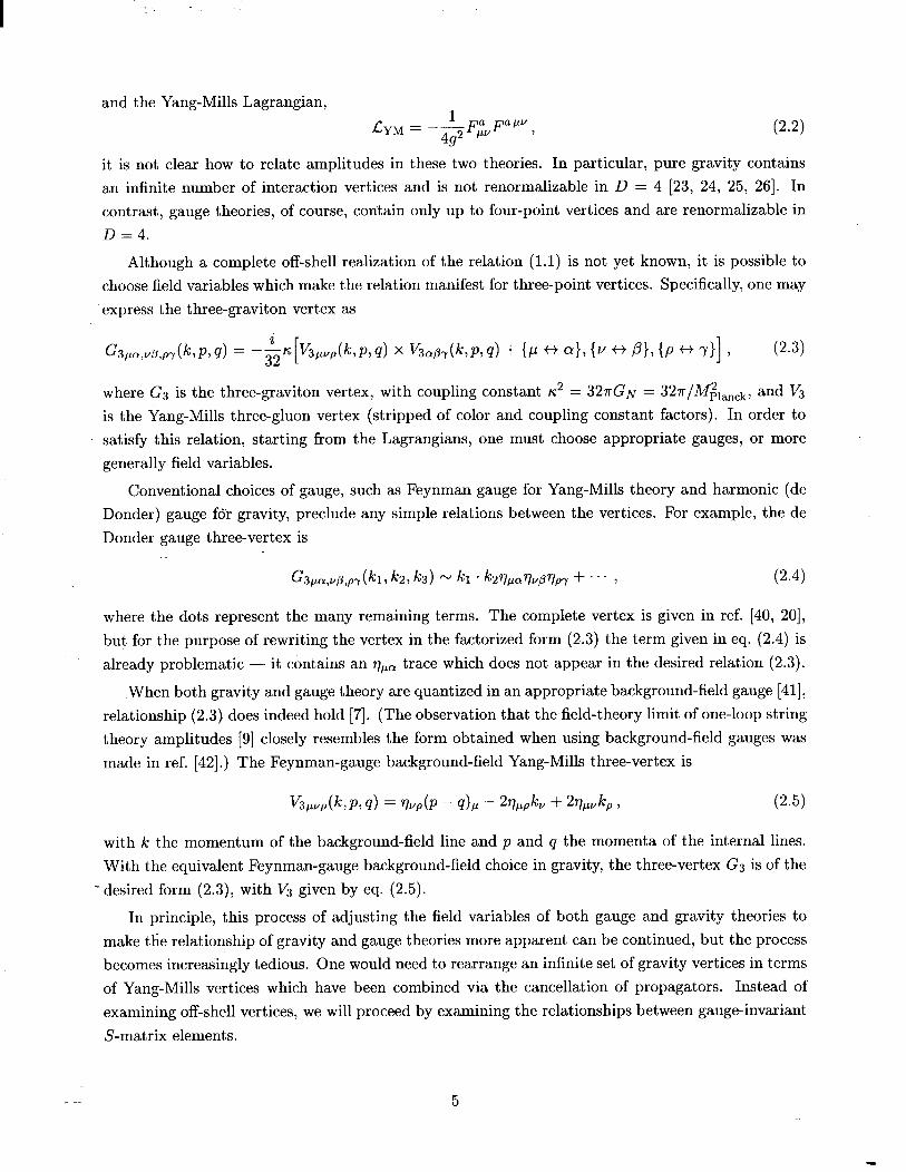
express the three-graviton vertex as
where GJ is the three-graviton vertex, with coupling constant K,’ = 321rG~ = 32~/M&,,,~, and V3
is the Yang-Mills three-gluon vertex (stripped of color and coupling constant factors). In order to
satisfy this relation, starting from the Lagrangians, one must choose appropriate gauges, or more
generally field variables.
Conventional choices of gauge, such as Feynman gauge for Yang-Mills theory and harmonic (de
Donder) gauge for gravity, preclude any simple relations between the vertices. For example, the de
Donder gauge three-vertex is
G 3pa,up,py(h, kz, kd N kl . hqpaqupqpy + . . . , (2.4)
where the dots represent the many remaining terms. The complete vertex is given in ref. [40, 201,
but for the purpose of rewriting the vertex in the factorized form (2.3) the term given in eq. (2.4) is
already problematic - it contains an qPcr trace which does not appear in the desired relation (2.3).
When both gravity and gauge theory are quantized in an appropriate background-field gauge [41],
relationship (2.3) does indeed hold [7]. (Th e o b servation that the field-theory limit of one-loop string
theory amplitudes [9] closely resembles the form obtained when using background-field gauges was
made in ref. [42].) The Feynman-gauge background-field Yang-Mills three-vertex is
Vbw(k~ P7 4) = q&J - q)p - 2qp,,k,, + 2+,k,, (2.5)
with k the momentum of the background-field line and p and q the momenta of the internal lines.
With the equivalent Feynman-gauge background-field choice in gravity, the three-vertex G3 is of the
- desired form (2.3), with V3 given by eq. (2.5).
In principle, this process of adjusting the field variables of both gauge and gravity theories to
make the relationship of gravity and gauge theories more apparent can be continued, but the process
becomes increasingly tedious. One would need to rearrange an infinite set of gravity vertices in terms
of Yang-Mills vertices which have been combined via the cancellation of propagators. Instead of
examining off-shell vertices, we will proceed by examining the relationships between gauge-invariant
S-matrix elements.
5
2.2 Kawai-Lewellen-Tye Tree-Level Relations
At tree-level, KLT have given a complete description of the relationship between closed string ampli-
tudes and open string amplitudes. This relationship arises because any closed string vertex operator
is a product of open string vertex operators,
V closed _ vopen j.7$; . - left (2.6)
The left and right string oscillators appearing in veft and Vri,, are distinct, but the zero mode
momentum is shared. This property of the string vertex operators is then reflected in the amplitudes.
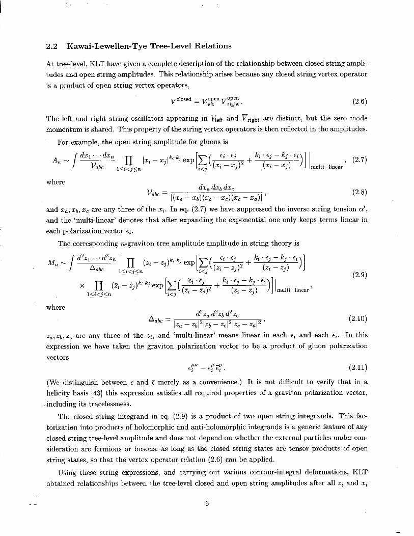
For example, the open string amplitude for gluons is
An N s
dxl . . . dx,
V abc n l<i<j<n
Ixi - xjlki’kj exP[g ((5ti zjj2 + Ici (j: 12,’ ‘i,] lmulti~linear, (2.7)
where
Vabc = 1(x, - xb;;;bd’:;& - 2,) 1 ’ (2.8)
and x,, Xb, x, are any three of the xi. In eq. (2.7) we have suppressed the inverse string tension a’,
and the ‘multi-linear’ denotes that after expanding the exponential one only keeps terms linear in
each polarization-vector ei.
The corresponding n-graviton tree amplitude amplitude in string theory is
Mn N s
l<i<j<n
where
(2.9)
(2.10)
z,, Zb, x, are any three of the zi, and ‘multi-linear’ means linear in each ei and each i. In this
expression we have taken the graviton polarization vector to be a product of gluon polarization
vectors
Ey II $z;. (2.11)
(We distinguish between E and c merely as a convenience.) It is not difficult to verify that in a
helicity basis [43] this expression satisfies all required properties of a graviton polarization vector,
_ including its tracelessness.
The closed string integrand in eq. (2.9) is a product of two open string integrands. This fac-
torization into products of holomorphic and anti-holomorphic integrands is a generic feature of any
closed string tree-level amplitude and does not depend on whether the external particles under con-
sideration are fermions or bosons, as long as the closed string states are tensor products of open
string states, so that the vertex operator relation (2.6) can be applied.
Using these string expressions, and carrying out various contour-integral deformations, KLT
obtained relationships between the tree-level closed and open string amplitudes after all zi and xi
6

integrations have been performed. In ref. [3] the KLT relations were used to obtain explicit formulae
for field-theory n-point MHV graviton amplitudes at tree level. After taking the field-theory limit,
the KLT relations for four- and five-point amplitudes are,
Miree(l,2,3,4) = - is12At4’““(1,2,3,4) Ap(1,2,4,3), (2.12)
Miree(l,2,3,4,5) = . ~r2~34Ap(l, 2,3,4,5)Ap (2,1,4,3,5)
+ iS13S24At;ee( 1,3,2,4,5) Ay(3,1,4,2,5) , (2.13)
where the M,‘s are the amplitudes in a gravity theory stripped of couplings, the An’s are the color-
bordered amplitudes in a gauge theory and .sij E (ki + k.j)2. We have suppressed all ej polarizations
and kj momenta, but have kept the ‘j’ labels to distinguish the external legs. These combine to give
the full amplitude via,
Ic. (n-2) Mp(l,2,...n) = 2
0 M?(l) 2,. . . n) ,
dp(lJ,...n) = g(+ c Tr(Tau(Wa4 . ..~~uc~.)A~(~(l),~(2),...,~(~)), 6%/Z,
(2.14)
where S,/Z, is the set of all permutations, but with cyclic rotations removed. The Tai are
fundamental representation matrices for the Yang-Mills gauge group SU(N,), normalized so that
Tr(TaTb) = Sab. (F or more detail on the tree and one-loop color ordering of gauge theory amplitudes
see refs. .[44, 451.) Our-phase conventions differ from those of ref. [3] in that we have introduced an
‘i’ into the gravity tree amplitudes; this is to maintain consistency with Minkowski-space Feynman
rules. In the sewing procedure, which we use in later sections, these phases are unimportant, since
one can anyway fix phases at the end of the calculation.
-It is sometimes convenient to write the four-point Yang-Mills amplitude in terms of structure
constants as
dt,‘ee(l, 2,3,4) = g2 [ f”a2a3c~a1A~(l, 2,3,4) + plagcf”caqa2Atqree(2, 1,3,4) 1 , (2.15)
where
f”abc = ifif abc = Tr( pa, Tb]TC) ) (2.16)
and U(1) decoupling and reflection identities [44] have been used.
The relations (2.12) and (2.13) hold for any external states of a closed string and not just
gravitons. We can thus obtain the amplitudes containing, for example, gravitinos:
M,t’ee(lh,2hr3h,4/J = - &Ap(Ig, 2,, 3,,4,) Ap(lg, 2,, 4~73,) , (2.17)
In this equation we have labeled the particle types of the N = 8 multiplet, graviton (h), spin-3/2
gravitino (h), vector (v), spin-l/2 fermion (G) and scalar (s). The labels of the N = 4 Yang-Mills
multiplet are: gluon (g), gluino (3) and scalar (s). In general, a closed string state in four dimensions
with helicity X is composed of a ‘left’ state of helicity XL and a ‘right’ state of helicity XR, where
X = XL + XR. We can then obtain the gravity amplitudes for states of helicity {Xi} in terms of gauge
theory amplitudes with states of helicity {XL,~} and {XR,~} just as in eq. (2.17). In an arbitrary
7

dimension D, similar relations hold, where the N = 8 states are constructed as tensor products of
N = 4 states, in terms of representations of the massless little group SO(D - 2).
As a concrete example, consider the four gluon amplitude given by
where s = ~12, t = ~14 and u = ~13 are the usual Mandelstam variables and where the tensor ts is
defined in eq. (9.A.18) of ref. [5], except that the term containing the eight-dimensional Levi-Civita
tensor should be dropped. The kinematic factor K is totally symmetric under interchange of external
~legs. Applying the relation (2.12) yields the four-graviton amplitude
Miree(l,2,3,4) = =$.
A relation we will use later is
(2.19)
st~M;‘~~(l,2,3,4) = -i (~t[Ap(1,2,3,4)])~ . (2.20)
These expressions may be made more concrete in four dimensions. The only non-vanishing
four-gluon helicity amplitudes at tree-level (and at any loop order in supersymmetric Yang-Mills
theory [27]), are those with two positive and two negative gluon helicities. All of these configurations
are trivially related in N = 4 Yang-Mills theory. The one independent tree amplitude is . .
Ap(l-, 2-, 3+, 4+) = i (1 a4
(12) (2 3) (3 4) (4 1) ’ (2.21)
using the spinor helicity formalism [43] to represent the amplitudes. (The reader may wish to
consult review articles for details [44].) The f superscripts label the helicity of the external gluon.
In general, we will drop the g subscript from a gluon leg in A, and the h subscript from a graviton
leg in M,. We use the notation (ktyIkj+) = (ij) and (k+Iky) = [ij], where Ik’) are massless Weyl
spinors, labeled with the sign of the helicity and normalized by (i j) [j i] = sij = 2ki . kj. In this
formalism the one nonvanishing four-graviton tree amplitude is
Miree(l--, 2-, 3+, 4+) = -isi (1 a8
(1 2)2 (2 3) (2 4) (3 4)2 (3 1) (4 1) . (2.22)
We can rewrite these amplitudes in a form which clarifies the relationship between gauge and
gravity theories. Firstly we may rearrange the Yang-Mills result,
@=(I-, 2-, 3+, 4+) = -; x
Ap(l-,2-,4+,3+) = -1 x
u
(2.23)
We have chosen to write the amplitudes.as a pole times a non-singular term.
In gravity we expect all algebraic factors associated with vertices to be squares of corresponding
gauge theory factors. However, the propagators of gravity are the same propagators as in gauge
8

theory. This suggests that we can obtain the corresponding pure gravity amplitude by squaring all
kinematic factors in eq. (2.23) except for the poles and summing over permutations. As a test of
this expectation note that the gravity amplitude (2.22) can be rewritten in the form
(12) WI 2 - s[121 (34) ’ I (2.24)
where the coefficient of each pole is the square of the coefficients appearing in eq. (2.23). This
relationship may be expressed in terms of coefficients of 43 scalar diagrams as we have done in
fig. 1. (The value of the +3 scalar diagram in the upper left of fig. 1 is i/s.) From eqs. (2.23)
land (2.24) we can read off the coefficients of the 43 scalar diagrams for Ap(l-, 2-, 3+,4+) and
Miree(l-,2-,3+,4+):
c, =o, ct=cu=+# (2.25)
Similar relations hold for supergravity amplitudes where some of the gravitons are replaced by
other states, for example the amplitudes Mlree(l--XL-XR, 22,3+, 4+XL+XR) where the gauge theory
amplitudes are Ap (l-‘, 2-, 3+, 4+‘) and where
c, = 0, (4 2)
Ct=G= (m > 20-X) x
[ s (12) WI
[121(34)’ I (2.26)
Here Miree (l- ‘L-‘R, 2-, 3+,4SXL+XR) is a product of a ‘left’ gauge theory factor times a ‘right’
gauge theory factor depending on the decomposition of each state in the gravity theory in terms of
gauge theory states.
In the remaining sections of this paper, we shall argue that, at least for N = 8 supergravity,
similar relations hold to all loop orders.
Gauge Theory
Gravity
Figure 1: Tree-level gauge theory four-gluon amplitudes and gravity four-graviton amplitudes expressed in terms of scalar 43 diagrams. The coefficients of the graviton amplitudes are squares of the coefficients for four-gluon amplitudes.
2.3 Relationships between Loop Amplitudes
At one loop it is more difficult to take the field-theory limit of a string. Nevertheless, a technology
exists for systematically extracting such limits [9]. This approach was followed in refs. [7, 81 to
9
compute four-graviton amplitudes in a variety of supersymmetric and non-supersymmetric field
theories. A feature of these calculations is that at the very beginning the loop integrands for gravity
are products of two Yang-Mills integrands.
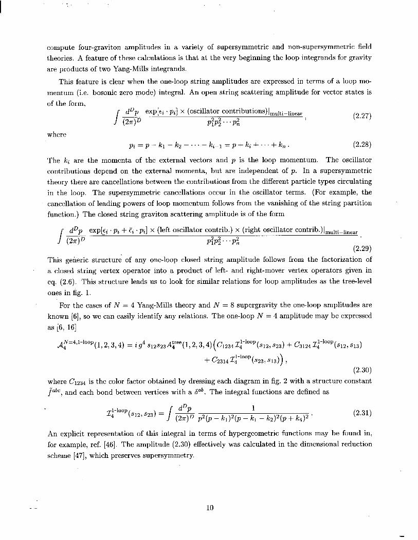
This feature is clear when the one-loop string amplitudes are expressed in terms of a loop mo-
mentum (i.e. bosonic zero mode) integral. An open string scattering amplitude for vector states is
of the form,
I
dDp exp[ei . pi] x (oscillator contributions) Imulti-linear
(24 D P:P;...PFl 7 (2.27)
where
pi = p - ICI - k2 - . . . - ki-l = p + ki + . . . + k, . (2.28)
The ki are the momenta of the external vectors and p is the loop momentum. The oscillator
contributions depend on the external momenta, but are independent of p. In a supersymmetric
theory there are cancellations between the contributions from the different particle types circulating
in the loop. The supersymmetric cancellations occur in the oscillator terms. (For example, the
cancellation of leading powers of loop momentum follows from the vanishing of the string partition
function.) The closed string graviton scattering amplitude is of the form
I dDp exp[_Ei . pi + pi . pi] x (left oscillator contrib.) x (right oscillator contrib.)ImultiPlinear
cwD PfP;-.Pi (2.29)
This generic structure of any one-loop closed string amplitude follows from the factorization of
a closed string vertex operator into a product of left- and right-mover vertex operators given in
eq. (2.6). This structure leads us to look for similar relations for loop amplitudes as the tree-level
ones in fig. 1.
For the cases of N = 4 Yang-Mills theory and N = 8 supergravity the one-loop amplitudes are
known [6], so we can easily identify any relations. The one-loop N = 4 amplitude may be expressed
as [6, 161
dr=411-100p (1,2,3,4) = i g4 Sl2S23Atqree(l, 2,3,4) ( 6234$100P(%2, s23) + c3124 $100p(s12; s13)
+ c2314 14 1-100p(s23is13)),
(2.30)
where Cl234 is the color factor obtained by dressing each diagram in fig. 2 with a structure constant
f labc, and each bond between vertices with a S ab The integral functions are defined as .
l-loop 14 (s12’ s23) = I
dDp
(27r)D p2(p - k#(p - il - k2)2(p + k4)2 * (2.31)
An explicit representation of this integral in terms of hypergeometric functions may be found in,
for example, ref. [46]. The amplitude (2.30) effectively was calculated in the dimensional reduction
scheme [47], which preserves supersymmetry.
10
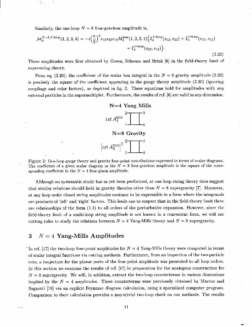
Similarly, the one-loop N = 8 four-graviton amplitude is,
Mr=811-100p (1,2,3,4) = -i(E)” S~2S23S~3M~ree(l,2r3,4)(~~-100P(~~2rS23) +~~-100p(S12,S13)
+ $100p(s23, s,,)) .
(2.32)
These amplitudes were first obtained by Green, Schwarz and Brink [6] in the field-theory limit of
superstring theory.
From eq. (2.20), the coefficient of the scalar box integral in the N = 8 gravity amplitude (2.32)
is precisely the square of the coefficient appearing in the gauge theory amplitude (2.30) (ignoring
couplings and color factors), as depicted in fig. 2. These equations hold for amplitudes with any
external particles in the supermultiplet. Furthermore, the results of ref. [6] are valid in any dimension.
N=4 Yang Mills
ist At4”” ‘_rr, 1 4
N=8 Gravity
istAp 2 2
III
3
Figure 2: One-loop gauge theory and gravity four-point contributions expressed in terms of scalar diagrams. The coefficient of a given scalar diagram in the N = 8 four-graviton amplitude is the square of the corre- sponding coefficient in the N = 4 four-gluon amplitude.
-Although no systematic study has as yet been performed, at one loop string theory does suggest
that similar relations should hold in gravity theories other than N = 8 supergravity [7]. Moreover,
at any loop order closed string amplitudes continue to be expressible in a form where the integrands
are products of ‘left’ and ‘right’ factors. This leads one to suspect that in the field-theory limit there
are relationships of the form (1.1) to all orders of the perturbative expansion. However, since the
field-theory limit of a multi-loop string amplitude is not known in a convenient form, we will use
cutting rules to study the relations between N = 4 Yang-Mills theory and N = 8 supergravity.
3 N = 4 Yang-Mills Amplitudes
-In ref. [17] the two-loop four-point amplitudes for N = 4 Yang-Mills theory were computed in terms
of scalar integral functions via cutting methods. Furthermore, from an inspection of the two-particle
cuts, a conjecture for the planar parts of the four-point amplitude was presented to all loop orders.
In this section we examine the results of ref. [17] in preparation for the analogous construction for
N = 8 supergravity. We will, in addition, extract the two-loop counterterms in various dimensions
implied by the N = 4 amplitudes. These counterterms were previously obtained by Marcus and
Sagnotti [19] via an explicit Feynman diagram calculation, using a specialized computer program.
Comparison to their calculation provides a non-trivial two-loop check on our methods. The results
11
:
of ref. [17] are more general, being the complete amplitudes and not just divergences. We also
comment that a comparison of the two calculations illustrates the computational efficiency of the
cutting techniques: the calculation of the complete amplitudes in terms of scalar integrals can easily
be performed without computer assistance. Moreover, the technicalities associated with overlapping
divergences are alleviated. We will apply the same cutting techniques to obtain new results for
N = 8 supergravity.
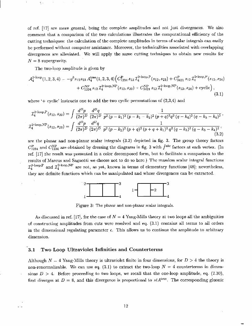
The two-loop amplitude is given by
d;-loop(l, 2,3,4) = - g6s12s23 Ap(l, 2,374) (cr234 S12Zq2-100P1P(S12~ S23) + cr42, S12~~-100p’p(S12, S24)
+ C,N,4 S12 14 2-100p’NP(S12, S23) + C$;r S~2~~-100p’NP(S~2, S24) + cyclic) ,
(3.1)
where ‘+ cyclic’ instructs one to add the two cyclic permutations of (2,3,4) and
z-loop~p I dDp dDq 1
(s12’s23)= ~~p2(p-k1)2(p-kl-k2)2(p+q)2q2(q-k4)2(q-k3-k4)2’
Z2-100p~Np(S12, 523) = I dDp dDq 1 - - 4
(WD WD p2 (P - W2 (P + cd2 (P + 4 + kd2 q2 (q - W2 (q - k3 - k4j2 ’
(3.2)
are the planar and non-planar scalar integrals (3.2) depicted in fig. 3. The group theory factors
c,P,34 and Cg54 are obtained by dressing the diagrams in fig. 3 with f”abc factors at each vertex. (In
ref. [17] the result was-presented in a color decomposed form, but to facilitate a comparison to the
results of Marcus and Sagnotti we choose not to do so here.) The massless scalar integral functions
z4 2-loop,P and z;-loop,NP are not, as yet, known in terms of elementary functions [48]; nevertheless,
they are definite functions which can be manipulated and whose divergences can be extracted.
Figure 3: The planar and non-planar scalar integrals
As discussed in ref. [17], for the case of N = 4 Yang-Mills theory at two loops all the ambiguities
of constructing amplitudes from cuts were resolved and eq. (3.1) contains all terms to all orders
in the dimensional regulating parameter E. This allows us to continue the amplitude to arbitrary
dimension.
-3.1 Two Loop Ultraviolet Infinities and Counterterms
Although N = 4 Yang-Mills theory is ultraviolet finite in four dimensions, for D > 4 the theory is
non-renormalizable. We can use eq. (3.1) t o extract the two-loop N = 4 counterterms in dimen-
sions D > 4. Before proceeding to two loops, we recall that the one-loop amplitude, eq. (2.30),
first diverges at D = 8, and this divergence is proportional to stAtree. The corresponding gluonic
12

:
counterterm is fixed by supersymmetry to be
t8F4 _ tpl~1p2V2~3?3p4~4p
8 ~lvl Fi2v2 F,&3 F$U4 Cabcd
= 4! F,aSFbPrF,c,Fdb” (
- $$pbffp~;6~d7” >
cabcd , (3.3)
where Cab& is a group theory factor (which we often suppress for clarity). In four dimensions we
can rewrite this term as
t8F4 = $(F - F)2(F + &)2 = ;(Fap - Fag) (F”” - gap) (Fr6 + &) (FYs + Fy6) , (3.4)
where F is the dual of F. The full counterterm also includes the scalar and fermionic operators
obtained by the N = 4 completion of the F4 terms [19]. The two-loop counterterms will be specified
in terms of derivatives acting on tgF4.
We may extract the coefficient of the counterterm from the ultraviolet divergences in our ampli-
tude. In general, to extract a counterterm from a two-loop amplitude one must take into account
sub-divergences and one-loop counterterms. Indeed, the divergences in ref. [19] received contribu-
tions from a large number of two-loop graphs with diverse topologies, many of which contained
sub-divergences (i.e. l/e2 poles) which required subtraction before the l/c poles could be extracted.
The cancellation of l/e poles in the D = 6 theory occurred only after summing all diagrams and
taking into account one-loop off-shell counterterms.
In our case, however, eq. (3.1) is manifestly finite in D = 6, since both planar and non-planar
double-box integrals first diverge in D = 7. The manifest finiteness in D = 6 is not an accident and
is due to the lack of off-shell sub-divergences when using on-shell cutting rules. It is also simple to
extract the D = 7 and D = 9 counterterms, which are the ones evaluated in ref. [19], by evaluating
the ultraviolet poles of the scalar integrals (3.2). The evaluation of these poles is performed in
appendix C.
The counterterm in D = 7 is of the form d2F4, as can be seen from dimensional analysis. The
form is again unique (at the on-shell linearized level)
t~1”1~2”2~3”3~4”4~~F~~U1~aF~2v2F~~v3F~4v4~~bcd, (3.5)
where C&,-d is another group theory factor. Again, in D = 4 such a tensor takes on a simple
schematic form,
(F - F)2a2(F + F)2. (3.6)
In the notation of Marcus and Sagnotti [19] the counterterm is presented as
TD (F,~F~~F,~F~~ - ~F,~F~“F,~F+ + . . j . (3.7)
From the expression (3.1) and appendix C we obtain
6 T7 = - (4z)F2e ’ [(
$j k%234 + cL43) + $j cf%4) + cYclic] ,
E [i&2 (-45s2 + l&t + 2t2) c,p,,, + & (-45~~ + 18s~ + 2u2) C,p,,, (3.8)
- + cyclic,
13

corresponding to the D = 7 and D = 9 counterterms.
To compare eq. (3.8) to the results of ref. [19] we must rearrange the group theory factors to
coincide with their basis. The necessary rearrangements are presented in appendix D. Comparing
eq. (D.2) with eqs. (4.5) and (4.6) of ref. [19] we find that all the relative factors agree (up to a
typographical error in eq. (4.6) in which the tree group theory factors accompanying the s3 and
t3 factors were exchanged). After accounting for a different normalization of the operator tgF4, as
deduced from the one-loop case, the overall factor for Tg also agrees, while our result for T7 is larger
than that in ref. [19] by a factor of 3/2. Nevertheless, the agreement of the relative factors is rather
T-on-trivial and provides a strong check that the amplitude in eq. (3.1) is correct.
3.2 Higher Loop Structure
As shown in ref. [17] the two-particle cut sewing equation is the same at any loop order, allowing
one to iterate the sewing algebra to all loop orders. As we discuss in section 5.2, the two-particle
cuts were performed to all orders in the dimensional regularization parameter E, and are therefore
valid in any dimension. However, since this construction is based only on two-particle cuts it is
only reliable for integral functions which can be built using such cuts. We call a function which is
successively two-particle reducible into a set of four-point trees ‘entirely two-particle constructible’.
Such contributions can be both planar and non-planar. (Planar topologies give the leading Yang-
Mills contributions for a large number of colors.) All two-loop contributions, and the three-loop
contributions shown in fig. 8, are entirely two-particle constructible. An example of a three-loop
non-planar graph which is not entirely two-particle constructible is given in fig. 4.
1 3
H 4
2
Figure 4: This three-loop non-planar graph is not entirely two-particle constructible. (In fact it has no two-particle cuts at all.)
The two-particle cut sewing equation leads to a loop-momentum factor insertion rule for planar
contributions [17], as shown in fig. 5. The pattern is that one takes each L-loop graph in the L-loop
amplitude and generates all the possible (L + 1)-loop graphs by inserting a new leg between each
possible pair of internal legs. Diagrams where triangle or bubble subgraphs are created should not
be included. The new loop momentum is integrated over, after including an additional factor of
i(er + e2)2 in the numerator, where !i and e2 are the momenta flowing through each of the legs to
which the new line is joined. (This rule is depicted in fig. 5). This procedure does not create any
four-point vertices. Each distinct (L+l)-loop contribution should be counted once, even though they
can be generated in multiple ways. (Contributions which have identical diagrammatic topologies but
different numerator factors should be counted as distinct.) The (L + 1)-loop amplitude is then the
sum of all distinct (L + 1)-loop graphs. This insertion rule has only been proven for the entirely
two-particle constructible contributions.’
For both the planar and non-planar entirely two-particle constructible contributions to the Yang-
14
e2 e2 ..-.. . .
+ i (& + 12)2 x ..-.. . . 1
. .
. . 4 4
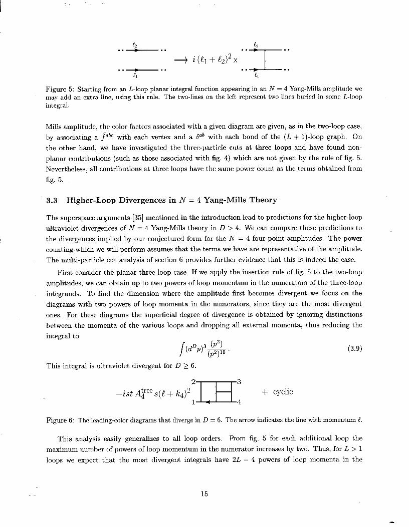
Figure 5: Starting from an L-loop planar integral function appearing in an N = 4 Yang-Mills amplitude we may add an extra line, using this rule. The two-lines on the left represent two lines buried in some L-loop integral.
Mills amplitude, the color factors associated with a given diagram are given, as in the two-loop case,
by associating a fabc with each vertex and a dab with each bond of the (L + 1)-loop graph. On
the other hand, we have investigated the three-particle cuts at three loops and have found non-
planar contributions (such as those associated with fig. 4) which are not given by the rule of fig. 5.
Nevertheless, all contributions at three loops have the same power count as the terms obtained from
fig. 5.
3.3 Higher-Loop Divergences in N = 4 Yang-Mills Theory
The superspace arguments [35] mentioned in the introduction lead to predictions for the higher-loop
ultraviolet divergences of N = 4 Yang-Mills theory in D > 4. We can compare these predictions to
the divergences implied by our conjectured form for the N = 4 four-point amplitudes. The power
counting-which we willperform assumes that the terms we have are representative of the amplitude.
The multi-particle cut analysis of section 6 provides further evidence that this is indeed the case.
First consider the planar three-loop case. If we apply the insertion rule of fig. 5 to the two-loop
amplitudes, we can obtain up to two powers of loop momentum in the numerators of the three-loop
integrands. To find the dimension where the amplitude first becomes divergent we focus on the
diagrams with two powers of loop momenta in the numerators, since they are the most divergent
ones. For these diagrams the superficial degree of divergence is obtained by ignoring distinctions
between the momenta of the various loops and dropping all external momenta, thus reducing the
integral to ”
s (d D 3 (P2>
4 @2)10 . (3.9)
This integral is ultraviolet divergent for D 2 6.
2 3
-id Ape s(l + k4)2 + cyclic 1 4
Figure 6: The leading-color diagrams that diverge in D = 6. The arrow indicates the line with momentum C.
This analysis easily generalizes to all loop orders. From fig. 5 for each additional loop the
maximum number of powers of loop momentum in the numerator increases by two. Thus, for L > 1
loops we expect that the most divergent integrals have 2L - 4 powers of loop momenta in the
15

Dimension D Loop Counterterm
8 1 F4
7 2 d2F4
6 3 d2F4
5 6 d2F4
Table 1: For N = 4 Yang-Mills theory in D dimensions, the number of loops at which the first ultraviolet divergence occurs for four-point amplitudes, and the generic form of the associated counterterm. In each case the degree of divergence is logarithmic, but the specific color factors will differ.
numerator. These integrals will reduce to
s
D L b2)(L-2) @ d (p2)3L+1 ’ (3.10)
(The L = 1 case is special and must be treated separately.) These integrals are finite for
D<;+4, (L > 1). (3.11)
This degree of dicergence is eight powers less than the maximum for non-supersymmetric Yang-Mills
theory.
This’iV = 4 power count has differences with the conventional one based on superspace argu-
ments [35]. Specifically, for dimensions D = 5,6 and 7 the amplitudes first diverge at L = 6,3 and
2 loops. The corresponding superspace arguments indicate that the first divergence may occur at
L = 4,3 and 2, respectively. Since the superspace arguments of ref. [35] only place a bound on finite-
ness, our results at four and five loops are not inconsistent. However, the ultraviolet behavior of the
amplitudes seems to indicate that the extra symmetries in N = 4 Yang-Mills theory, which are not
taken into account by the off-shell N = 2 superspace arguments, are important to understanding
its divergences in D > 4. Curiously, the finiteness condition (3.11) agrees with the power count
based on the assumption of the existence of an unconstrained off-shell covariant N = 4 superspace
formalism [38, 391. This agreement is probably accidental, because it is known that such a formalism
does not exist; for example, the two-loop D = 7 counterterm has the wrong group-theory structure
(although the right dimension) to be written as an N = 4 superspace integral [19].
Combining the N = 4 finiteness condition (3.11) with those for N = 1,2 [39] (for which off-shell
superspaces for the full supersymmetry exist) we find that an L > 1 loop amplitude is finite for
D< 2(N-1) +4 L )
N = 1,2,4. (3.12)
4 N = 8 Supergravity Amplitudes
In this section we present the exact result for the N = 8 two-loop four-point amplitude, in terms
of scalar integral functions. Moreover, we present a conjecture for a precise relationship between
16

(parts of) the N = 4 Yang-Mills and N = 8 supergravity four-point amplitudes to all loop orders,
extending the tree and one-loop relationships summarized in figs. 1 and 2.
Using the two-loop N = 4 Yang-Mills amplitudes discussed in the previous section, we can im-
mediately obtain candidate expressions for the corresponding N = 8 amplitudes simply by dropping
the color factors and squaring the coefficients and numerators of every scalar integral. In section 5.2
we will verify that this procedure is valid to all loop orders for the entirely two-particle constructible
terms. For the two-loop case, in section 5.3 we also evaluate the three-particle cuts, allowing for
a complete reconstruction of this amplitude, proving that the squaring procedure gives the correct
two-loop results. (Direct evaluations of the two- and three-particle cuts using the four-dimensional
helicity basis may be found in appendices A and B.)
4.1 Two-Loop N = 8 Supergravity Amplitudes
We now obtain the two-loop N = 8 four-graviton amplitudes by squaring the corresponding coef-
ficients appearing in the N = 4 four-point amplitudes (3.1), after stripping away the color factors.
The N = 8 amplitudes are thus expected to be,
M;-100P(1,2,3,4) = -i(;)“[ ~12~23 Ay(l,2, 3,4)12 (~~2J$~~~~‘~(S12, ~23) + ~~~~~~~~~~~~~~~~~ ~24)
+ st2 z4 2-100p’NP(S12, S23) + ST2 ~~-loop’NP(S~2r S24) + cyclic >
.
(4.1)
Here Ape is the N = 4 Yang-Mills four-gluon tree amplitude, the integrals are defined in eq. (3.2)
1 (see fig. 3) and ‘+ cyclic’ instructs one to add the two cyclic permutations of (2,3,4), just as in
eq. (3.1). Using eq. (2.20) we may re-express the overall coefficient in terms of the gravity tree
amplitude to obtain the final form for the amplitude,
M;-loop(l, 2,3,4) = (;)” s12s2ssis Mjree(l, 2,3,4) ($2 1;-100p’p(sr2, s23) + sf21~-100p’p(s12, 524)
2-loop,NP + ST2 14
2-loop,NP (s12,s23) + ST2 14 (s127S24) + cyclic .
(4.2)
N=4 Yang Mills
N=8 Gravity
Figure 7: The expected relationship between two-loop contributions to N = 8 four-graviton amplitudes and N = 4 four-gluon amplitudes: the graviton coefficients are squares of the gluon coefficients. The N = 4 and N = 8 contributions depicted here are to be multiplied respectively by factors of -g’stAp (dropping the
group theory factor) and -i(rC/2)6[stApe]2.
17

The two-loop ultraviolet divergences for N = 8 supergravity in D = 7, 9 and 11, after using the
results of appendix C and summing over the different double-box integrals which appear, are
M;-i~~~, D=7-2r I pole = 2E (&7 i(s’ + t2 + u2) x (;y x StUMqtree,
M;-loop, D=9-2tlpole = 1 -13n(g + t2 + g)2 x 4E (47r)9 9072 0
5 6 x StUIL!l;‘ee )
M;-loop, D=ll-2r~pole = 1 7r 486 (47r)‘l 5791500
(438(s6 + t6 + u6) - 53s2t2u2) x ($ x stuMqtree .
(4.3) There are no sub-divergences because one-loop divergences are absent in odd dimensions when using
dimensional regularization.
In all three cases, for four graviton external states, the linearized counterterms take the form of
derivatives acting on
plus the appropriate N = 8 completion. As mentioned in the introduction, the operator (4.4) appears
in the tree-level superstring effective action. It also appears as the one-loop counterterm for N = 8
supergravity in D = 8. Finally, it is thought to appear in the M-theory one-loop effective action
[49]. .- -
4.2 Higher-loop conjecture
We conjecture that to all orders in the perturbative expansion the four-point N = 8 supergravity
amplitude may be found by squaring the coefficients and numerator factors of all the loop integrals
that appear in the N = 4 Yang-Mills amplitude at the same order, after stripping away the color
factors. In section 5 we show that the exact two-particle cuts and the two-loop three-particle cuts
confirm this picture, making the conjecture precise at two loops.
In order to specify the precise form of the conjecture at L loops one would need to investigate
cuts with up to (L + 1) intermediate particles. Nevertheless, some of the integral coefficients and
numerators can be obtained from the known two-particle cuts. For example, fig. 8 contains a
few sample three-loop integrals which are entirely two-particle constructible, and their associated
coefficients for the case of N = 4 Yang-Mills theory [17]; the N = 8 supergravity coefficients are
-given by squaring the super-Yang-Mills coefficients. This provides an explicit example of three-loop
relationships between contributions to the Yang-Mills and gravity amplitudes for the cases of N = 4
and N k 8 supersymmetry. The supergravity coefficients can again be expressed in terms of the
tree-level gravity amplitudes using eq. (2.20). It would be interesting to determine whether squaring
relations do indeed continue to hold for all remaining three-loop diagram topologies.
18

N=4 Yang Mills
s= :m; s(! + kq)= :r+rI
N=8 Gravity
Figure 8: Some sample three-loop integrals and their coefficients for N = 4 Yang-Mills theory and for N = 8 supergravity. The coefficients for iV = 8 supergravity are just the squares of those for N = 4 Yang-Mills theory. The N = 4 and N = 8 contributions depicted here are to be multiplied respectively by overall factors of -ig8stAlf’= and (~/2)*[stAy]~.
4.3 Higher-Loop Divergences in N = 8 Supergravity
In this subsection we discuss the ultraviolet behavior of N = 8 supergravity arising from our all-
loop conjecture for the form of the four-point amplitude. This ‘squaring’ conjecture gives twice as
many powers of loop momentum in the numerator of the integrand as for Yang-Mills theory. The
power-counting equation that describes the leading divergent behavior for N = 4 Yang-Mills theory,
eq.. (3.10), becomes for N = 8 supergravity at L loops,
s
D L (p2)w-2)
cd d @2)3L+l ’
This integral will be finite when
(4.5)
The results of this analysis are summarized in table 2. In particular, in D = 4 no three-loop
divergence appears - contrary to expectations from a superspace analysis [36, 351 - and the first
R4-type counterterm occurs at five loops. The divergence will have the same kinematical structure
- as the D = 7 divergence in eq. (4.3), but with a different non-vanishing numerical coefficient.
The one- and two-loop entries in table 2 are based on complete calculations of the amplitudes.
Beyond- two loops we do not have complete calculations, but in section 5.2 we will show that the
divergence structure given in eq. (4.6) is consistent with the two-particle cuts to all loop orders,
and in section 6 we will demonstrate related ultraviolet cancellations in the m-particle MHV cuts.
Continuing along these lines, a complete proof of the ultraviolet behavior of the L-loop amplitude
would require an analysis of all contributions to the cuts.
19

Dimension Loop Degree of Divergence
8 1 logarithmic
7 2 logarithmic
6 3 quadratic
5 4 quadratic
4 5 logarithmic
Counterterm
R4
tY4R4
9R4
9R4
a4R4
Table 2: The relationship between dimensionality and the number of loops at which the first ultraviolet diver- gence should occur in the N = 8 supergravity four-point amplitude. The form of the associated counterterm assumes the use of dimensional regularization.
5 Cut Constructions
In this section we justify the form of the N = 8 four-point amplitude presented in section 4 by
iterating the exact D-dimensional two-particle cuts to all loop orders. We will also compute the
D-dimensional three-particle cuts at two loops, demonstrating that eq. (4.2) gives the complete two-
loop N = 8 amplitude. First we briefly review the cut construction method [12, 13, 16, 17, 151 for
constructing complete amplitudes. This approach leads to relatively compact expressions because
the calculation is organized in terms of gauge-invariant quantities at intermediate steps.
In this method the-amplitude is reconstructed from its analytic properties. In general, to recon-
struct an L-loop amplitude one must calculate all cuts, which can have up to (L + 1) intermediate
states. However, the various cuts are related to each other, so one can often write down complete
expressions for the amplitudes based on a calculation of a small subset of cuts. (When combining
the cuts into a single function, care must be exercised not to over-count a particular term.) Once
one has a robust ansatz for the form of the amplitude, the remaining cuts become much easier to
calculate, since one has a definite final form to compare with. As one calculates additional cuts, one
obtains cross-checks on the terms inferred from the earlier cuts; the consistency of the different cuts
provides a rather powerful check that one is calculating correctly.
We find it convenient to perform the cut construction using components instead of superfields.
The potential advantage of a superfield formalism would be that one would simultaneously include
contributions from all particles in a supersymmetry multiplet. However, for the cases we investigate,
the supersymmetry Ward identities, discussed in appendix E, are sufficiently powerful that once the
contribution from one component is known the others immediately follow. In a sense these identities
are equivalent to using an on-shell superspace formulation. A component formulation is also more
natural for extensions to non-supersymmetric theories.
5.1 Review of Cut Construction Method
As an example, consider the cut construction method for a two-loop amplitude JU~-‘~~~(~, 2,3,4).
At two loops one must consider both two- and three-particle cuts. In each channel there can be
multiple contributing cuts. For example, in the s channel there are two two-particle cuts, as depicted
20
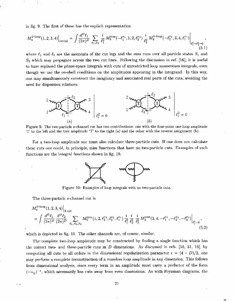
in fig. 9. The first of these has the explicit representation
M2-100p(L 4 2, 3,4)Icutcaj = 1% c SlJ2
;M;‘““(-e~1,1,2,e;Z) 1
~M41-1oop(-e~2,3,4,es’) 2
I 7 eq=e;=o
(5.1) where er and f$ are the momenta of the cut legs and the sum runs over all particle states Sr and
S2 which may propagate across the two cut lines. Following the discussion in ref. [16], it is useful
to have replaced the phase-space integrals with cuts of unrestricted loop momentum integrals, even
though we use the on-shell conditions on the amplitudes appearing in the integrand. In this way,
one may simultaneously construct the imaginary and associated real parts of the cuts, avoiding the
need for dispersion relations.
(4 (b) Figure 9: The two-particle s-channel cut has two contributions: one with the four-point one-loop amplitude ‘1’ to the left and the tree amplitude ‘T’ to the right (a) and the other with the reverse assignment (b).
For a-two-loop amplitude one must also calculate three-particle cuts. If one does not calculate
these cuts one could, in principle, miss functions that have no two-particle cuts. Examples of such
functions are the integral functions shown in fig. 10.
Figure 10: Examples of loop integrals with no two-particle cuts.
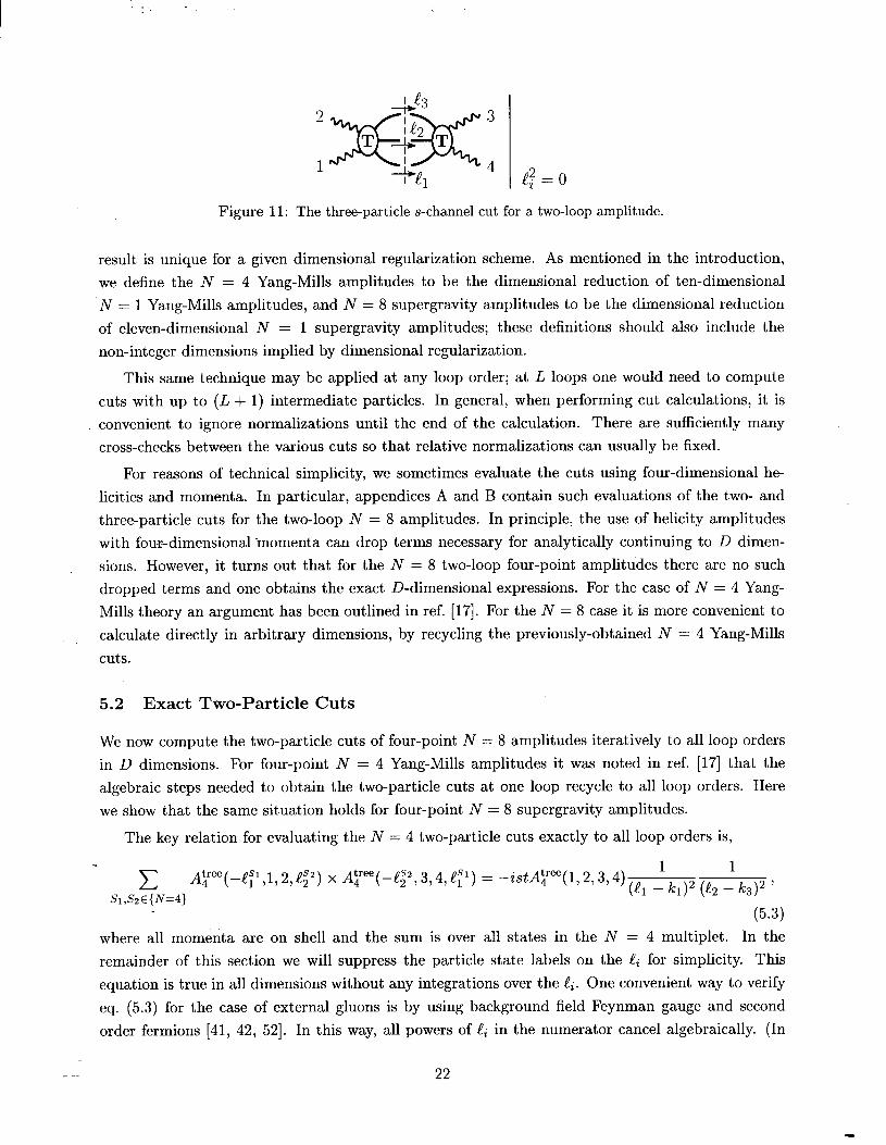
The three-particle s-channel cut is
~2-100pP,2, 3,4)13-c”t 4
I dDel dDez . . .
= (2T)D (2n)D sl~s,M,t’ee(l,2,e~3,e~Z,e:‘l) i i ~M,t’ee(3,4,-e~l~-ezS”:-e~3) ejl=o>
(5.2) which is depicted in fig. 11. The other channels are, of course, similar.
The-complete two-loop amplitude may be constructed by finding a single function which has
the correct two- and three-particle cuts in D dimensions. As discussed in refs. [50, 51, 161, by
computing all cuts to all orders in the dimensional regularization parameter E = (4 - D)/2, one
may perform a complete reconstruction of a massless loop amplitude in any dimension. This follows
from dimensional analysis, since every term in an amplitude must carry a prefactor of the form
(-~ij)-~, which necessarily has cuts away from even dimensions. As with Feynman diagrams, the
21
:-Jg==k I e2 3
-AT
’ 4 4 ez = 0
Figure 11: The three-particle s-channel cut for a two-loop amplitude.
result is unique for a given dimensional regularization scheme. As mentioned in the introduction,
we define the N = 4 Yang-Mills amplitudes to be the dimensional reduction of ten-dimensional
N = 1 Yang-Mills amplitudes, and N = 8 supergravity amplitudes to be the dimensional reduction
of eleven-dimensional N = 1 supergravity amplitudes; these definitions should also include the
non-integer dimensions implied by dimensional regularization.
This same technique may be applied at any loop order; at L loops one would need to compute
cuts with up to (L + 1) intermediate particles. In general, when performing cut calculations, it is
convenient to ignore normalizations until the end of the calculation. There are sufficiently many
cross-checks between the various cuts so that relative normalizations can usually be fixed.
For reasons of technical simplicity, we sometimes evaluate the cuts using four-dimensional he-
licities and momenta. In particular, appendices A and B contain such evaluations of the two- and
three-particle cuts for the two-loop N = 8 amplitudes. In principle, the use of helicity amplitudes
with four-dimensional -momenta can drop terms necessary for analytically continuing to D dimen-
sions. However, it turns out that for the N = 8 two-loop four-point amplitudes there are no such
dropped terms and one obtains the exact D-dimensional expressions. For the case of N = 4 Yang-
Mills theory an argument has been outlined in ref. [17]. For the N = 8 case it is more convenient to
calculate directly in arbitrary dimensions, by recycling the previously-obtained N = 4 Yang-Mills
cuts.
5.2 Exact Two-Particle Cuts
We now compute the two-particle cuts of four-point N = 8 amplitudes iteratively to all loop orders
in D dimensions. For four-point N = 4 Yang-Mills amplitudes it was noted in ref. [17] that the
algebraic steps needed to obtain the two-particle cuts at one loop recycle to all loop orders. Here
we show that the same situation holds for four-point N = 8 supergravity amplitudes.
The key relation for evaluating the N = 4 two-particle cuts exactly to all loop orders is,
c Ap(-e;l,l,2,e;2) x A~(-e;~,3,4,ql) = -istAp(l,2,3,4) S1,SzE{N=4}
(5.3)
where all momenta are on shell and the sum is over all states in the N = 4 multiplet. In the
remainder of this section we will suppress the particle state labels on the .$ for simplicity. This
equation is true in all dimensions without any integrations over the !i. One convenient way to verify
eq. (5.3) for the case of external gluons is by using background field Feynman gauge and second
order fermions [41, 42, 521. In this way, all powers of .f$ in the numerator cancel algebraically. (In
22

this particular scheme eq. (5.3) is true even for off-shell .$.) The uniqueness of the supersymmetric
completion of the operator given in eq. (3.3) assures that one obtains an A? no matter what the
external states are.
Using the KLT relation (2.12) we can use eq. (5.3) to obtain the equivalent relation for N = 8
supergravity,
C hgy-el, i,2, e2) x hfp(-e2, 3,4, el) N=8 states
= -s 2 C &y-el,i,2,e2) x At,‘ee(-e2,3,4,el) N=4 states >
+4p(e2, I, 2, -el) x @yel, 3,4, -e,)
= ~~(st)~[Ap(l, 2,3, 4)12 (4 - hw2 - k3Ae2 + hwl + k3)2
= i~~stz&f;~~~(l,2,3,4) (el - k1)2(e2 - k3)2:el - k2)2(e2 - k4)2 .
(5.4) In eq. (5.4) we have used the decomposition of a state in the N = 8 multiplet into a ‘left’ and a ‘right’
N = 4 state, and the fact that summing over the N = 8 multiplet is equivalent to summing over the
left and right N = 4 multiplets independently. We then perform a partial-fraction decomposition of
the denominators (using the on-shell conditions), . .
- (el - lc1)2:el - k2)2 = (e, -il)2 +
- (e, - k$(e, - k4)2 = (e, Ag)2 + (e2 La)2 ’
P-5)
to obtain the N = 8 basic two-particle on-shell sewing relation,
c hfpy-el, i,2,e2) x bf,ty-e2,3,4,e,) N=8 states
I[ 1 (e, : k3)2 + (e2 _ k4)2 1
(5.6)
7
where the ei are on-shell. The t- and u-channel formulas are given by relabelings of the legs in
eq. (5.6). From this sewing relation it is trivial to obtain the N = 8 one-loop amplitude (2.32).
A key feature of the sewing relation (5.6) is that when one sews two tree amplitudes and sums
over all intermediate N = 8 states, one gets back a tree amplitude multiplied by scalar functions.
-This means that we may recycle the sewing relation (5.6) to obtain two-particle cuts of higher-loop
amplitudes. The only difference is that now we must track the scalar function prefactors.
Consider, for example, the two-particle s-cut with a tree amplitude on the left and a one-loop
amplitude on the right,
M2-100p(l,2,3,4)(_~“t= 1% -x 4 $@ee(-&J,2,&) ~~~~100p(-~~~3~4~~l)/12=y2=o~ N-8 states l
l z(5.7)
23
Inserting eq. (2.32) for i’Hi-loop and applying the sewing relation (5.6), we have
~~~~~~~~~~ 2,3, 4)1s-cUt= -StUb!f;ree / $$S(e2 - k3)2(& - k4)2
x [$lOOP cs, (e2 - k3j2) + zql+OP ((e2 - k3J2, (e, - k4J2) + zql+JOP w2 - k4)5 41 112X9 =. 7
l(5!8)
where we have combined the two propagators on a common denominator in the second brackets
in order to make a cancellation manifest. The unwanted propagators cancel and our final result is
remarkably simple,
iV~-lOOp(l, 2,3, 4)lsmcut = stUM;rees2 (zq2-1°0pQ t) + X;-loop,p(s, U)
+ ~~-100p7~P (S) t) + z;-100p7NP (s, ?A)) 1 s-cut ) (5.9)
where the scalar integrals Zi-loop’p and Z~-loop’NP are defined in eq. (3.2). The analysis of the
two-particle t- and u-channel cuts is identical.
It is simple to_ find a single function with the correct two-particle cuts in all three channels; the
answer is given in eq. (4.2). We emphasize that the results for the two-particle cuts are valid in
any dimension and do not rely on any four-dimensional properties. (A more direct evaluation of the .- two-particle cuts using four-dimensional helicity states may be found in appendix A.)
Since the right-hand side of sewing relation (5.6) is proportional to the tree amplitude, one may
iterate this procedure to obtain the ‘entirely two-particle constructible’ contributions, defined in
section 3.2, at any desired loop order.
5.3 Two-loop Three-Particle Cuts
We now evaluate the D-dimensional two-loop three-particle cuts for the N = 8 four-point amplitude,
by recycling the analogous calculation for N = 4 Yang-Mills theory. (In appendix B we also evaluate
the N = 8 three-particle cuts directly, using the helicity formalism, which yields the same result.)
Consider first the three-particle s-channel cut (5.2). Just as for the two-particle sewing, the
sum over three-particle states for N = 8 supergravity may be expressed as a double sum over
N = 4 states. Then we may apply the five-point KLT formula (2.13), which expresses the N = 8
_ supergravity tree amplitudes appearing in eq. (5.2) in terms of the corresponding N = 4 Yang-Mills
tree amplitudes.
The. tree amplitude on the left side of the cut is
2M,tyel,i,2,e3,e2) =i(el+k1)2(e3+k2)2A~(el,1,2,e3,e2)At;ee(l,el,e3,2,e2)+(1 ~21, * (5.10)
where we have chosen a convenient representation in terms of the gauge theory amplitudes. (The
(1 +) 2) interchange acts only on Icr and k2, and not on !r and f!z.) Similarly, for the tree amplitude
24

I _
on the right side of the cut,
~;‘~~(-e~, 3,4, -e,, 4,) = i (e, - k3)2(ll - kq)2Ap(-ls, 3,4, -l,, -&) At;ee(3, -[3, -e,, 4, -&)
+ (3 * 4). (5.11)
Thus we have,
c ~~ree(l,2,e3,e2,el)M5t’ee(3,4,-el,-e2,-e3) N=8 states
= -(e, + kl)2(e3 + k2)2(e3 - k3)2(4 - k4)2
x [
c A?&, 1,2,t&)A~(-&,3,4, -t,, -t,) N=4 states 1
x c A~(l,el,e3,2,e2)A~(3, -e3, -el,4, -e2) N=4 states 1
+ (1 * 2) + (3 +) 4) + (1 * 2, 3 t) 4))
(5.12)
where all momenta are to be taken on-shell. The sum over N = 4 states in each set of brackets
can be simplified using the results for the two-loop N = 4 Yang-Mills amplitudes (3.1). Taking the
three-particle cuts of the planar contributions (see figure 3 of ref. [17]) yields the on-shell phase-space
integral of -
x [ (t-1 - k4)2([3 + k2)&, + l2)2@2 + !3)2 + (es - k3)2(G + &l + e2)2(e2 + e3)2
+ (e, - k3)2(& - k4)2(e, + k2)2(4 + k1)2 1 .
(5.13)
This equation actually holds even before carrying out the loop-momentum (or phase-space) integral.
In the calculations used to derive the results of ref. [17] eq. (5.13) was obtained at the level of the
integrands, with all states carrying four-dimensional momenta and helicities, but then it was argued
that the light-cone superspace power-counting of Mandelstam [53] ruled out corrections coming from
the (-2e)-dimensional components of the loop momenta. Since this argument is based on superspace
cancellations it applies to the integrands before integration over loop momenta, and works for D-
dimensional external states as well. (A similar argument is also applied in appendix B.4.)
The second sum over N = 4 states is similar, but more complicated, involving three different
25

cuts of planar double-boxes and ten of non-planar ones,
c Atjee(l,el,e3,2,e2)A~(3,-e3,-el,4,-e2) = -istAp(1,2,3,4) N=4 states
x [ - (4 + [3)2@3 + k2)2;a + k1)2(& - k3)2 + (h + W2(!2 + li2)2t(ez - k3)2(& - k4)2
+ (el + h)2(e3 + k2& - k4)2(e2 - k3)2 - (& + e3)2(e2 + k2)2:e3 - k3)2(h - k4)2
+ (el + kl)2(&? + k2)2t(el - k4)2@3 - k3)2 + (h + h)2(e3 + k2):(& - k4)2([3 - k3)2
-
(12 + kl)2(!3 + k2)22;11 - k4)2(e2 - k3)2 - (h + e3)2(e2 + h)2:13 - k3)2(& - k4)2
+ (e, + kl)2(!3 + b2)2t(!3 - k3)2(& - k4)2 - (6 + e3)2(h + h)2b3 + k2)2(e2 - k4)2
-
(el + 1kl)~(!2 + k2)2;!3 - k3)2(!2 - k4)2 + (cl + kd2(e3 + k2)‘(e3 - k3)2(e2 - k4)2
t + 1
(e2 + h)2(e3 + k2)2(e3 - k3)2(e2 - k4)2-’ ’ (5.14)
The complete
eq. (5.12).
N = 8 result is given by simply inserting the N = 4 results (5.13) and (5.14) into
I e3 2 3
1 I e, -X 2
E I e,
l I 4
I 2
t3
3 lI lx
--
Figure 12: The three-particle s-channel cuts for gravity. We must also sum over 1 +) 2, 3 +) 4 and the 3! permutations of er, es and es. We have included the appropriate combinatoric factors necessary for eliminating double counts.
This may be compared with the s-channel three-particle cuts of eq. (4.2). Taking all s-channel
26

three-particle cuts of the scalar integrals, as shown in fig. 12, we obtain
stuMiree I dDel dDe2 1 -- (24D (240 eq e; e;
{K
1 t2 t2 X
5 (el + k#(e3 + kg(e3 - k#(el - k4)2 + (e2 + k#(e3 + k#(e3 - k#(el - k4)2
s2 1 s2
+ (el + e2w2 + e3w3 + k2)wl - k4)2 + 5 (e2 + e3)2(e3 + k1)2(e2 + k2)2(e1 - k4)2
1 s2 + 5 (e, + e2)2(e3 + k2)2(e2 - k3)2(el - k4)2 > + perms(el’ e2’ “) 1
+ (1 +) 2) + (3 * 4) + (1 +) 2, 3 +) 4) e;=o ’
(5.15)
where we have included all kinematic factors associated with each scalar diagram in fig. 12. The
1 t) 2 and 3 +) 4 permutations act on all terms in the square brackets. Note that the cut result
(5.12) also contains a sum over 1 t) 2 and 3 +) 4 interchanges.
We have verified that the expressions in eqs. (5.15) and (5.12) are indeed equal. The t- and
u-channel cuts are identical, up to relabelings. Since all two- and three-particle cuts are correctly
given by eq. (4.2) in arbitrary dimensions, it is the complete expression for the two-loop four-point
N = 8 supergravity amplitude, expressed in terms of scalar loop integrals.
6 Supersymmetric Cancellations in MHV Cuts to All Loop Orders
In this section we illustrate four-dimensional supersymmetric cancellations that take place at any
loop order, in all cuts where the amplitudes on both sides of the cut are maximally helicity violating
(MHV). The MHV contributions are the most tractable, which is why we focus on them. Supersym-
metry Ward identities only relate amplitudes with the same total helicity; thus when considering
supersymmetric cancellations the MHV contributions do not mix with the non-MHV contributions.
This section provides a concrete demonstration of the role that the SWI’s play in reducing the degree
of divergence of supersymmetric S-matrix elements. For MHV cuts at any loop order we will obtain
the same supersymmetric reduction in powers of loop momentum as we obtained in the entirely two-
particle constructible contributions, providing additional evidence that the power-counting formulas
(3.11) and (4.6) hold.
As a warm-up, we will first consider the case of N = 4 Yang-Mills theory. Since the supersym-
- metry identities of N = 8 supergravity are closely related to those of N = 4 Yang-Mills theory, it is
relatively simple to extend the N = 4 analysis to N = 8 supergravity.
27
6.1 N = 4 Yang-Mills Theory Warm-up
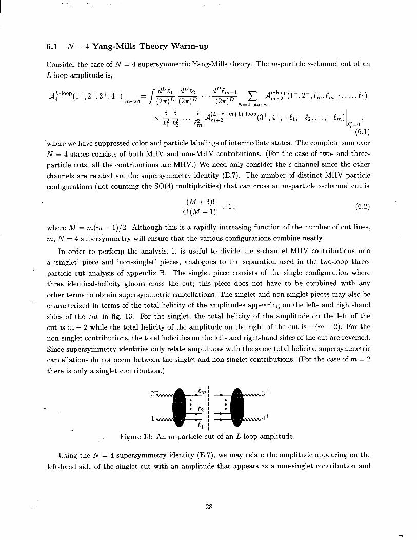
Consider the case of N = 4 supersymmetric Yang-Mills theory. The m-particle s-channel cut of an
L-loop amplitude is,
At-looP(l-, 2- d;$p(i-,2-,e,,e,-l,. . . ,el)
i i - d~;;-mfl)-loop (3+, 4+, 4,) -e2, . . . , -em) ’ jTE *.. e2
m e$o ’
(6.1)
where we have suppressed color and particle labelings of intermediate states. The complete sum over
N = 4 states consists of both MHV and non-MHV contributions. (For the case of two- and three-
particle cuts, all the contributions are MHV.) We need only consider the s-channel since the other
channels are related via the supersymmetry identity (E.7). Th e number of distinct MHV particle
configurations (not counting the SO(4) multiplicities) that can cross an m-particle s-channel cut is
(M+3)1 +1 4!(M-l)! ’ (64
where M = m(m - 1)/2. Although this is a rapidly increasing function of the number of cut lines,
m, N = 4 supersymmetry will ensure that the various configurations combine neatly.
In order to perform the analysis, it is useful to divide the s-channel MHV contributions into .- a ‘singlet’ piece and ‘non-singlet’ pieces, analogous to the separation used in the two-loop three-
particle cut analysis of appendix B. The singlet piece consists of the single configuration where
three identical-helicity gluons cross the cut; this piece does not have to be combined with any
other terms to obtain supersymmetric cancellations. The singlet and non-singlet pieces may also be
characterized in terms of the total helicity of the amplitudes appearing on the left- and right-hand
sides of the cut in fig. 13. For the singlet, the total helicity of the amplitude on the left of the
cut is m - 2 while the total helicity of the amplitude on the right of the cut is -(rn - 2). For the
non-singlet contributions, the total helicities on the left- and right-hand sides of the cut are reversed.
Since supersymmetry identities only relate amplitudes with the same total helicity, supersymmetric
cancellations do not occur between the singlet and non-singlet contributions. (For the case of m = 2
there is only a singlet contribution.)
Figure 13: An m-particle cut of an L-loop amplitude.
Using the N = 4 supersymmetry identity (E.7), we may relate the amplitude appearing on the
left-hand side of the singlet cut with an amplitude that appears as a non-singlet contribution and
28

exhibits no supersymmetric cancellation by itself,
d,+2(i-,2-,e;,...e~) = (1 a4 --[dm+2(i-,2-,ey- ,..., ei_,,e;,e;+, ,..., q,,e;,e;+, ,..., e;)]+, (4 ei)4
(6.3) where the dagger means that we interchange (o b) +) [ba]. A similar identity holds for the amplitude
appearing on the right-hand side of the singlet cut. This explicitly shows that we may extract a
factor of (1 2)4 [3 414 f rom the singlet cut, as compared to a contribution with no supersymmetric
cancellations.
More interestingly, the sum over non-singlet contributions exhibits a cancellation dictated by the
supersymmetry Ward identities. Table 7 of appendix E contains the relative SW1 factors between
the amplitudes that appear on the right-hand side of the cuts. In table 3 we have collected the
various types of contributions to the non-singlet MHV cuts; all remaining such contributions are
given by relabelings. Each entry in the first column of table 3 is obtained by multiplying one of the
23 entries in table 7 with the conjugate factor from the amplitude on the left-hand side of the cut.
(The conjugate amplitudes with two cut fermion lines have an additional minus sign, making up for
the fermion loop sign.)
Collecting all MHV non-singlet contributions together yields an overall factor of
(2 )
4 4 aij =s (6.4)
in the amplitude, where aij = (& +$)” = 2& .Q. Equation (6.4) is an explicit all-loop demonstration
of the reduction in powers of loop momentum implied by supersymmetry. The SW1 (E.7) implies
that the same types of cancellations occur for the t- and u-channel cuts, although different states
cross the cuts.
6.2 Supersymmetry Cancellations in N = 8 Supergravity
The analysis of the m-particle cuts at L loops for the case of N = 8 supergravity is quite similar
to that of N = 4 Yang-Mills theory. For N = 8 supergravity, the total number of distinct MHV
particle configurations that can cross the cut is,
(M+7)! +1 8!(M- l)! ’ (6.5)
-where M = m(m - 1)/2. These MHV contributions to the m-particle cuts can again be divided into
singlet and non-singlet contributions, characterized by the total helicity of the amplitudes appearing
on either side of the cuts. For the singlet, the total helicity of the amplitude on the left side of the
cut is 2(m - 2), while the total helicity of the amplitude on the right of the cut is -2(m - 2). For
the non-singlet contributions, the total helicities on the left and right sides of the cut are reversed.
As for N = 4 Yang-Mills theory, the simplest case to consider is the singlet where m identical-
helicity gravitons cross the cut. For the singlet, the SW1 (E.11) implies that one can extract the
factor (12)’ [3 418 f rom the cut integrand as compared to a factor of (& $)’ [& .Q18 for a pure graviton
29

Relative Factor Multiplicity
a!2 1
I a;2a34 I aT2a23 I 4
a;2034056 ,
aLa23a45 , ‘$2a34a45 I 42a23a34
&a23a14, af2a23al3 I a;2al3al4
a12a34a56a78, a12a23a45a67,
a12a23a34a56, a12a23a45a56, a12a23a13a45
a12a23a34a45, a12a23a34a41 , a12a13a14a56
12
24
Table 3: The relative numerator factors dictated by the supersymmetry Ward identities, arising from the non-singlet sewing of two MHV N = 4 Yang-Mills amplitudes, where aij = (& + .Q)‘. The 23 different terms in the left column of the table correspond to the 23 different particle configurations in table 7, which contains the relative factor for the amplitude on the right-hand side of the cut.
contribution to the non-singlet. Note that these factors are the squares of the corresponding N = 4
Yang-Mills factors. _ . .
For the non-singlet case to which all remaining MHV configurations contribute, we need to
combine the various terms in order to obtain a reduction in the degree of divergence. An easy way
to determine the relative factors between amplitudes appearing on either side of the non-singlet
cut is from the KLT relations on tree amplitudes. For (m + 2)-point gravity tree amplitudes these
relations are of the form
M:t2(i,2,el ,..., e,) - c(II( >
ep+e,)2 A~~,O,eil ,..., ei,,2,ei,+l ,..., 4,) {WI m-l factors (6.6)
x A~2(1,eil,...,eik,2,eik+l,...,ei,),
where {ir, ip, . . . ,k} and {.b,.h,. . . , jm} are permutations of { 3,4, . . . , m + 2) which are determined
from the KLT expressions. Since the relative factors for any MHV N = 4 tree amplitude are known
from the SWI, the KLT relations (6.6) immediately imply that they are known for any MHV N = 8
tree amplitude. Furthermore, since the supersymmetry Ward identities hold to all orders of the
_ perturbative expansion, the relative factors determined in this way are the same ones that appear at
loop level. A more direct analysis using the N = 8 Ward identities yields the same relative factors.
After including the appropriate multiplicity factors, following the previous discussion for N = 4
Yang-Mills theory, again we may combine all relative factors in the non-singlet MHV s-channel cuts
to obtain an overall factor of
(2 )
8
aij = s8 ) (6.7)
which may be extracted from the cut integral. The symmetry under permutations of external legs
30

implied by the SW1 (E.ll) guarantees that one can also extract the same factor from the t- and
u-channel MHV cuts.
In summary, the above analysis illustrates that supersymmetry cancellations in the MHV cuts
occur to all loop orders, for the cases of N = 4 Yang-Mills theory and N = 8 supergravity. In
fact, these cancellations are closely related to those for the two-particle sewing relations, when one
negative gluon helicity appears on each side of the cut. (See eq. (5.6) of ref. [12].) Since these sewing
relations led to the power-counting eqs. (3.11) and (4.6), the MHV results presented in this section
suggest that these power counts hold more generally.
7 Conclusions
In this paper we investigated the relationship between gravity and gauge theory S-matrix elements.
Supergravity theories are interesting because they have softer ultraviolet behavior than ordinary
gravity theories and also appear in the low-energy limit of superstring theories. We chose to inves-
tigate the case of maximally supersymmetric theories (i.e. N = 4 Yang-Mills theory and N = 8
supergravity); such theories are heavily constrained and their amplitudes are therefore relatively
simple.
At tree and one-loop level the four-point amplitudes for N = 4 Yang-Mills theory and N = 8
supergravity exhibit a ‘squaring’ relationship (summarized in figs. 1 and 2). One of the results
contained in this paper is a complete calculation of the N = 8 two-loop four-point amplitude in
terms of scalar integrals, similar to the two-loop N = 4 Yang-Mills calculation performed in ref. [17].
From these amplitudes we have obtained the ultraviolet divergences in D = 7,9,11, and have shown
that the squaring relationship persists to two loops (as depicted in fig. 7). Motivated by these results
and by the structure of string amplitudes, we postulate that a similar relationship will extend to all
loop orders.
Evidence for this conjecture is provided by cutting techniques [12, 13, 16, 171, which allow a
complete analytic reconstruction of an L-loop amplitude, if one computes all possible cuts, up to
and including the (L + 1)-particle cuts. For the N = 8 four-point amplitude we have iterated the
one- and two-loop two-particle cut analysis to all loop orders. To do this we used the known [2, 31
relationship between gravity and gauge theory tree amplitudes to recycle the previous calculation
of the N = 4 Yang-Mills cuts [17]. Further checks of the conjecture could be provided by cuts
with more intermediate states, though this becomes increasingly difficult. Nevertheless, the cutting
method is overwhelmingly simpler than a corresponding Feynman diagram calculation.
Of supergravity theories, N = 8 is believed to have the softest ultraviolet behavior, so a com-
plete proof that it actually does diverge in four dimensions would provide strong evidence that all
supergravity theories are divergent. Although superspace power-counting arguments [35] suggest
the existence of a three-loop D = 4 counterterm, its presence has never been verified in an actual
calculation. Our results indicate that for N = 4 Yang-Mills theory and for N = 8 supergravity these
superspace power-counting arguments were too conservative regarding the possible cancellation of
infinities. In particular, our computation of the N = 8 two-loop amplitudes prove that there is no
31

counterterm in D = 5, contrary to expectations from superspace power counting [36, 351.
Furthermore, in four dimensions our cut calculations indicate, but do not yet prove, that there is
no three-loop counterterm for N = 8 supergravity, contrary to expectations from superspace power-
counting bounds. On the other hand, from the two-particle cuts we infer a counterterm at five loops
with non-vanishing coefficient. In order to have a complete proof that the divergence detected at five
loops does not cancel, one would need to investigate the cuts with up to six intermediate particles.
Alternatively, if one could prove that the numerators of all N = 8 loop-momentum integrals are
squares of the corresponding ones for N = 4 Yang-Mills integrals (i.e. they always appear with the
same sign), there would be no need for a detailed investigation of the cuts; we have shown that
the iterated two-particle cuts have the required squaring property. It would also be of interest to
directly verify whether or not the coefficient of the three-loop counterterm vanishes for the case of
N = 1 supergravity. It should be possible to address these and other issues with the methods used
in this paper.
Throughout the calculations presented in this paper we have found simple relationships between
N = 4 Yang-Mills theory and N = 8 supergravity. Without fail we have been able to exploit the
N = 4 Yang-Mills results to streamline N = 8 supergravity calculations. It would be interesting
to investigate whether such relationships between gravity and gauge theories can be found for cases
with less than the maximal supersymmetry.
Ackpowledgements
We thank K.S. Stelle for a number of important discussions and for encouragement. We also
thank S. Deser, S. Ferrara, R. Kallosh, D.A. Kosower, E. Marcus, and E.T. Tomboulis for discussions.
A. Two-particle Cuts Via Helicity
In this appendix we obtain the two-particle sewing equation (5.6) using a helicity basis. Four-
dimensional helicity methods make explicit calculations quite a bit easier, especially when the mo-
menta also reside in four dimensions. However, restricting the momenta in the cuts to four dimensions
may in principle drop terms necessary for continuation to other dimensions. Nonetheless, the four-
dimensional calculation makes the formal proof of eq. (5.6) transparent and gives us the opportunity
to introduce the notation which we use in the following appendix, where we calculate the two-loop
three-particle cuts using a helicity basis.
In four dimensions a massless external particle will have either positive or negative helicity. The
-four-graviton tree amplitudes Miree( l+, 2+, 3+, 4+) and Mjree( l-, 2+, 3+, 4+) vanish for all particle
types. This can be seen from eq. (2.12), since the corresponding gauge theory amplitudes vanish. For
a supergravity theory, this vanishing is true not just at tree-level, but at each order in perturbation
theory, due to supersymmetric Ward identities [27]. Thus, the only independent (under relabelings)
non-zero four-graviton amplitude is M4 (l- ,2-, 3+, 4+).
Therefore, in the sewing equation (5:6) we need only consider a single helicity configuration for
the external legs, which for convenience, we take to be (l-, 22,3’,4+). There are three possible
32
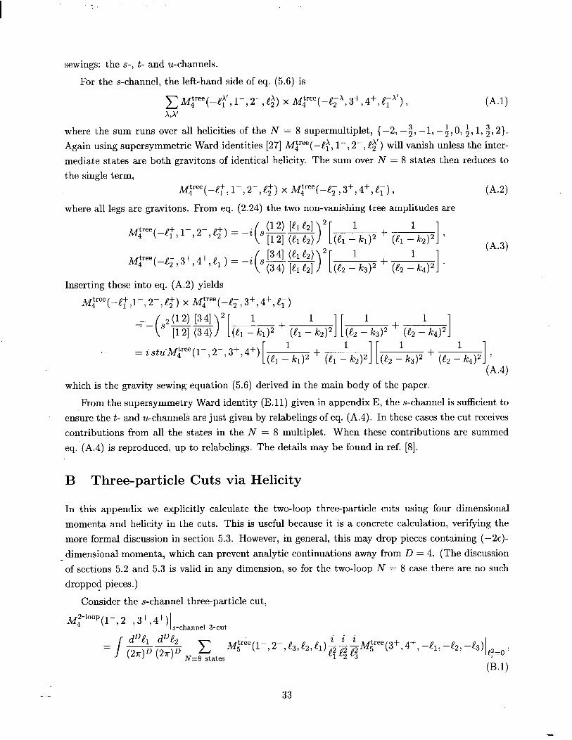
-_
sewings: the s-, t- and u-channels.
For the s-channel, the left-hand side of eq. (5.6) is
CMjree(-e:‘, 1-,a-,@> x ~~ree(--llpX,3+,4+,e;X’), X,X
(A4
where the sum runs over all helicities of the N = 8 supermultiplet, (-2, -g, -1, -i, 0, $, 1, g, 2}.
Again using supersymmetric Ward identities [27] Miree(-@, l-, 2-, e$‘) will vanish unless the inter-
mediate states are both gravitons of identical helicity. The sum over N = 8 states then reduces to
the single term,
Mjree(-e;, l-,2-&) x M;‘ee(-e;,3+,4+,e,))
where all legs are gravitons. From eq. (2.24) the two non-vanishing tree amplitudes are
(A4
M;ree(-e;,1-,2-,e;) = -i ( s(12) Lele21 2 [12l(ele,> >[ (el Jkl)2 + (e, llcz)’ ’ 1
( s[341 2 )[ (k$ Ikj)l + (45 Jka)2 * 1
64.3) j@ree(-e;,3+,4+,eq) = -i (3 4) [h !,I
Inserting these into eq. (A.2) yields
M4tree(-e;,l-,2-,Q) x M4tr”“(-!.;,3+,4+,e,)
- ( 2(W[3 2 1 =-- s- [12] (34) Ii (h - Q2 I[ (l, Jk3)2 + (e2 -i)z 1
. . = istu-M~‘ee(l-,2-,3+,4+) (el lklJ2 + (e, : k2J2 I[ (& :ksJ2 + (l, Ihq)Z ’ 1 (A4
which is the gravity sewing equation (5.6) derived in the main body of the paper.
From the supersymmetry Ward identity (E.ll) g iven in appendix E, the s-channel is sufficient to
ensure the t- and u-channels are just given by relabelings of eq. (A.4). In these cases the cut receives
contributions from all the states in the N = 8 multiplet. When these contributions are summed
eq. (A.4) is reproduced, up to relabelings. The details may be found in ref. [8].
B Three-particle Cuts via Helicity
In this appendix we explicitly calculate the two-loop three-particle cuts using four dimensional
momenta and helicity in the cuts. This is useful because it is a concrete calculation, verifying the
more formal discussion in section 5.3. However, in general, this may drop pieces containing (-2e)-
dimensional momenta, which can prevent analytic continuations away from D = 4. (The discussion
of sections 5.2 and 5.3 is valid in any dimension, so for the two-loop N = 8 case there are no such
dropped pieces.)
Consider the s-channel three-particle cut,
= J -- ~~‘ee(l-,2-,&3,e,,~~)~~~ e2 e2 e2@ree(3+,4+, -!I, 427 -e3)11T=o > 1 2 3
(i3.1)
33
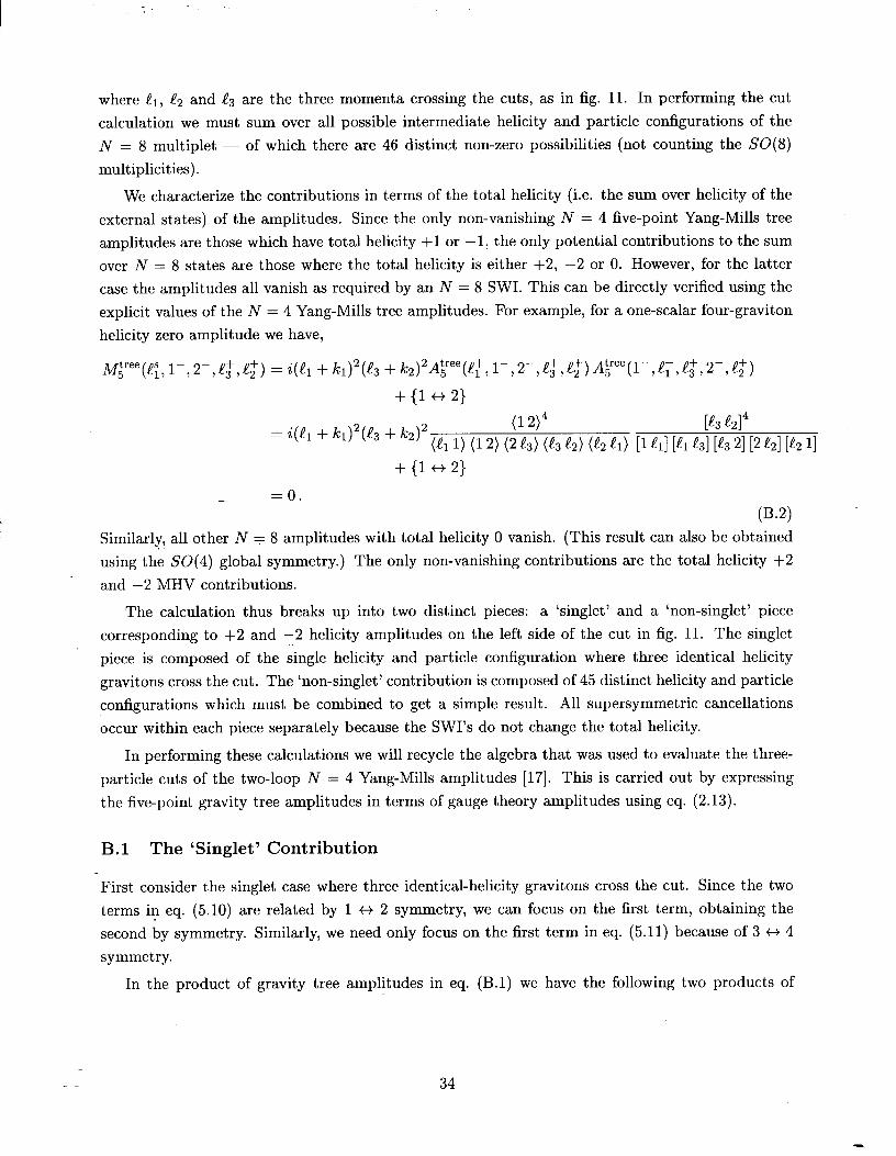
where !I, f?z and es are the three momenta crossing the cuts, as in fig. 11. In performing the cut
calculation we must sum over all possible intermediate helicity and particle configurations of the
N = 8 multiplet - of which there are 46 distinct non-zero possibilities (not counting the SO(8)
multiplicities).
We characterize the contributions in terms of the total helicity (i.e. the sum over helicity of the
external states) of the amplitudes. Since the only non-vanishing N = 4 five-point Yang-Mills tree
amplitudes are those which have total helicity +l or -1, the only potential contributions to the sum
over N = 8 states are those where the total helicity is either +2, -2 or 0. However, for the latter
case the amplitudes all vanish as required by an N = 8 SWI. This can be directly verified using the
explicit values of the N = 4 Yang-Mills tree amplitudes. For example, for a one-scalar four-graviton
helicity zero amplitude we have,
~~ree(es,i-,2-,e~,e2+) = ice, + k1)2(e3 + k2)2Ap(eT, 1-,2-,e~,e~)A~(i-,el,e3$,2-,e~)
+ (1 * 2)
= ice, + k1)2(e3 + k2)2 (1 2j4 [e3 e2i4 (4 1) (12) (2 e3) v3 e2) (e2 4) [led vl e31 v3 21[2 e21 [e2 13
+ (1 +) 2)
I.= 0.
(B.2) Similarly, all other N - 8 amplitudes with total helicity 0 vanish. (This result can also be obtained
using the SO(4) global symmetry.) The only non-vanishing contributions are the total helicity +2
and -2 MHV contributions.
The calculation thus breaks up into two distinct pieces: a ‘singlet’ and a ‘non-singlet’ piece
corresponding to +2 and -2 helicity amplitudes on the left side of the cut in fig. 11. The singlet
piece is composed of the single helicity and particle configuration where three identical helicity
gravitons cross the cut. The ‘non-singlet’ contribution is composed of 45 distinct helicity and particle
configurations which must be combined to get a simple result. All supersymmetric cancellations
occur within each piece separately because the SWI’s do not change the total helicity.
In performing these calculations we will recycle the algebra that was used to evaluate the three-
particle cuts of the two-loop N = 4 Yang-Mills amplitudes [17]. This is carried out by expressing
the five-point gravity tree amplitudes in terms of gauge theory amplitudes using eq. (2.13).
B.l The ‘Singlet’ Contribution
First consider the singlet case where three identical-helicity gravitons cross the cut. Since the two
terms in eq. (5.10) are related by 1 +) 2 symmetry, we can focus on the first term, obtaining the
second by symmetry. Similarly, we need only focus on the first term in eq. (5.11) because of 3 t) 4
symmetry.
In the product of gravity tree amplitudes in eq. (B.l) we have the following two products of
34

I -
Yang-Mills tree amplitudes
(a) Ap(i-,2-,e;,e;,e;) x Atjee(3+,4+,-el,-ez,-e,),
(b) Atjee(l-,e;&,2-,e2$) x Ap(3+,-&-e;,4+,-eiJ. (B.3)
These products have already been evaluated in the computation of the N = 4 Yang-Mills ampli-
tudes [17]. To evaluate the product (a) we use the explicit forms of the Yang-Mills amplitudes,
Ap(i-,2-,e;,ez+,e;) = i (1 2j4
(12) W3) (e3 e2) (e2 ed (4 1) 7
WI4 Atjee(3+, 4+, -e,, -e;, -e;) = -i [341[4 -41 L-4 -e,l i-e2 -e,] L-e, 31 7
(B.4)
giving,
A,Zy-(i-,2-,e;,e;,e; ) x ~tjee(3+, 4+, -e;, -ey, -e;)
= - (12)2 [3412 tr+[ie143e32]
(el + e2)2(e2 + e3)2(e3 - k3)2(el - k4)2(e3 + k2)2(el + k1)2 ’ P.5)
where tr+[ler ...I = tr[(l + ys) $1 qr . ..]/2. Similarly, for the product (b),
Atjee(i-,e;,e;;2-,e;) x Atjee(3+,-e3,-el,4+,-e2)
(1 2)2 [3412 tr+[l.C143e22] tr+[le243e32]
= --(el + e3)2(e1 + k1)2(13 + Ic$ye2 + k#(ez + k#(e3 - k#(el - k4)2(& - k#(e2 - k3)2 . 03.6)
Putting together the type (a) and type (b) contributions with the prefactors contained in
eqs. (5.10) and (5.11) we therefore have for the singlet contributions to the cut (B.l),
@-100p(l-,2-,3+,4+)/singlet 3-cut = stuMjree(l--,2--,3+,4+) J $$,$$
x tr+[ler43e321er43e221e243e32]
eq e; e; (e, - k3)2(el - k4)2(e3 + k2)2(el + kg (e, + e2)2(e2 + e3)2 1 (B.7)
’ (4 + e3w2 + k2w2 + k1)2(e2 - k4w2 - k3)2
+ (1 +) 2) + (3 +) 4) + (1 t) 2, 3 * 4) II ep=o ’
where we used
tr+[le143e32] tr+[le143e22] tr+[le243e32] = tr+[ie143e32ie143e22ie243e32]. P.8)
This completes the calculation of the singlet contribution. (The identical particle phase-space factor
of l/3! is canceled by the 3! permutations of the ei.) After combining this result with the non-singlet
contribution, computed in the following subsection, we will compare the total with the three-particle
cuts of the final form of the amplitude, eq. (4.2).
35

B.2 The Non-Singlet Contribution
We now include the sum over all remaining helicity and particle configurations that can cross the
cut. As we shall see, there are a total of 45 ‘non-singlet’ contributions which combine to give a
contribution which is almost identical to the singlet case. The first step in computing the cuts is to
organize the set of tree amplitudes that will contribute.
A simple way to obtain these tree amplitudes is via the KLT relations (5.10) and (5.11). The fac-
torizations of the required gravity tree amplitudes into gauge theory partial amplitudes via eq. (5.10)
are collected in the second and fourth columns of table 4. The third and fifth columns contain the
relative factors between the various gauge theory amplitudes. The pure gluon amplitude is
Atjee(3+,4+,el,e;,e3+) = i (4 e2)4 (3 4) (4 ed (6 e,) (e2 e3) (e3 3) *
(B.9)
The entry in the first row and third column of table 4 corresponds to the factor (er e2)4 appearing
in the numerator. As discussed in appendix E, the relative factors between the various amplitudes
are easily obtained via supersymmetry Ward identities [27] and are same ones used in the N = 4
Yang-Mills two-loop calculation [17]. F or example, from supersymmetry Ward identities we have
(ele2) Atjee(3+,4+,e;,ey,e$) = i (4 e2)3 (4 e3) (3 4) (4ed (el e2) (e2 e3) v3 3) 7
(B.lO)
whose numerator corresponds to the entry in the second row and third column of table 4.
Table 4: Factorization of N = 8 supergravity amplitudes into sums of products of N = 4 Yang-Mills - amplitudes. The factors in the third and fifth columns are the relative numerator factors appearing in the
gauge theory amplitudes. The corresponding factors in the supergravity cases are products of the ‘left’ and ‘right’ gauge theory amplitudes.
One nice property of using the KLT relations to obtain the gravity tree amplitudes is that we do
not need to use the N = 8 Lagrangian or Feynman rules. As a check, we have independently verified
the results for the gravity amplitudes contained in table 4 using the N = 8 supersymmetry algebra;
the product of each ‘left’ and ‘right’ factor contained in table 4 corresponds to the supersymmetry
Ward identity factor contained in table 8 in appendix E.
36

We comment that there is some ambiguity as to how to perform the factorization. For example,
left and right can be interchanged. As a less trivial example, the last entry in table 4 can be factorized
as h+h+v-v-G- +g+g+s-@-s- x g+s+#-s-g-. (B.ll)
However, in each case where an alternate factorization is available, it leads to the same overall factor
as the factorization in table 4, after the left and right factors are multiplied together, and ignoring
an irrelevant phase. (This ambiguity in factorizing arises because a string is composed of different
‘sectors’, such as the Ramond or Neveu-Schwarz sectors.)
When calculating the non-singlet contributions to the cut in eq. (B.l), we first evaluate the
case of three gravitons crossing the cut, and later use table 4 to obtain the remaining non-singlet
contributions. Just as in the singlet case, we may recycle a Yang-Mills calculation. Here we have to
evaluate the following products of tree amplitudes,
(a) Ay(i-,2-,e;,e;,e;) x A~(3+,4+,-el,-e2,-e~),
(b) AF(l-,e;t,&,2-,e2+) x A~(3+,-e~,-el,4+,-ez); (B.12)
again these products have already been evaluated in the analogous cut-calculation for N = 4 Yang-
Mills theory [17].
The net resukis that for h-h-h+ crossing the cut we obtain
M2-100p(l-,2-,3+,pf)~~on-singlet 3-cut = stu~;ree(l-,2-,3+,4+) I$$,$$ (el +s:)16 4 . .
’
tr-[Ier43e32Ur43e221e243e32]
eq e; e; (e, - k3)2(el - k4)2(e3 + k2)2(e1 + k1)2 (el + e2)2(e2 + e3)2
’ (e, + e3)2(e2 + k2)2(e2 ikl)2(& - k4)2(-% - kd2
+ (1 +-+ 2) + (3 * 4) + (1 +-+ 2, 3 * 4) 1
. ego
(B.13)
This result is exactly the one for the singlet except that tr+ -+ tr- and there is a prefactor of
((4 + e2)W.
We use table 4 to find the contribution of any other particle and helicity configuration from
eq. (B.13). (I n all cases, the helicity assignments are for particles that cross the cut from right to
left.) One simply multiplies each ‘left’ and ‘right’ relative factor in the table together and then
by their complex conjugate to obtain the total relative factors in the cuts. In table 5 we have
collected the relative factors between the various contributions to the cuts. All other non-vanishing
-contributions may be obtained by simple relabelings of the entries in the table.
Summing over all contributions that cross the cut, with the N = 8 multiplicities, we have
a8 + 8 a7c + 28 u6c2 + 56 u5c3 + 70 u4c4 + 56 a6bc + 168 a5bc2 + 280 a4bc3 + 420 a4b2c2 + 560 a3b2c3
+ relabelings, (B.14)
where u = (el + e2j2, b = (e, + e3J2 and c = (er + .&)2. This may be recombined to give
(u + b + c)8 = s8. (B.15)
37

1 Intermediate States 1 Relative Cut Factor
h-h-h+ a8 h-h-h+ 8 a7c
h-v-v+ h-j-j-e+
28 a6c2
56 a5c3
v-v-s+ _----
v v v
420 a4 b2c2
560 a3 b2c3
Table 5: The relative contributions to the non-singlet three-particle cuts obtained from taking the absolute value squared of the product of the ‘left’ and ‘right’ factors in table 4. The numbers appearing in the second column are the multiplicities for each type of cut. In the table a = (.Cr +e~)~, b = (a2 +t~)~ and c = (!r +.CS)~.
The factor of s8 exactly cancels the l/s8 appearing in eq. (B.13). Thus, after summing over all -. ‘non-singlet’ states crossing the cut, we obtain exactly the same result as for the singlet given in
eq. (B.13), except that.tr+ is replaced with tr-. Of course, since the 75 terms vanish for four-point
kinematics the results are actually completely identical, after loop-momentum integration. The net
effect is simply to double the singlet result.
B.3 Comparison to Ansatz
In order to verify that the cut results agree with the expression in eq. (5.15), we must compare the
integrands, eqs. (5.15) and (B.7), after accounting for the factor of two arising from combining the
singlet and non-singlet contributions. We have verified that the results are indeed equal. (When
evaluating the traces analytically one must account for the fact that det(ki . kj) vanishes in four
dimensions for five or more independent momenta. The analysis of section 5.3, which uses D-
dimensional expressions for the N = 4 Yang-Mills cuts as input, does not require the use of this
four-dimensional constraint.)
The t- and u-channel three-particle cuts may be evaluated similarly. However, it is much simpler
to appeal to the supersymmetry Ward identity (E.ll) which guarantees that the t- and u-channel
-cuts are identical to the s-channel cut, up to relabelings. Combining these results with those of
appendix A shows that eq. (4.2) is consistent with all cuts, but with D-dimensional momenta replaced
with four-dimensional ones.
B.4 Exactness of Cut Calculation
We now argue that although the previous cut calculations use spinor helicity with four-dimensional
cut momenta, no terms were dropped. In principle, we may have dropped pieces containing (--2e)-
38

dimensional momenta of the form,
J d4p d-2&, d4q d-2’p4 f (p, q, W x {cl;, & PP . PC.. -) --
(27r)4 (27r--2E (27r)4 (27r-26 (P2 - P;4h2 - P$ . . . ’ (B.16)
where we have explicitly separated the loop momenta into four- and (-2e)-dimensional parts. The
(-2e)-dimensional components of the two loop momenta are pp and pq. (A discussion of the (--2c)-
dimensional parts of loop momenta can be found, for example, in refs. [54, 511.) Terms containing
such factors are necessarily suppressed by a power of E. However, this suppression may be cancelled
if the integrals contain poles in E.
To avoid the need for an explicit calculation of contributions of the form (B.16), we make use of
the KLT tree-level relations which relate the tree amplitudes on either side of the three-particle cuts
to the ones appearing in the N = 4 cut calculation. In ref. [17] it was argued that the light-cone
superspace power-counting of Mandelstam [53] ruled out the appearance of terms of the form (B.16)
in the two-loop N = 4 three-particle cut sewing algebra. Since this argument is based on superspace
cancellations it applies to the integrands before integration over loop momenta.
Our observation here is rather simple: Since the N = 4 Yang-Mills sewing algebra using four-
dimensional momenta in the cuts is exact, then the N = 8 sewing algebra must also be exact since
it is composed of-sums of products of the N = 4 algebra. Thus there can be no terms of the form
(B.16) in the N = 8 supergravity sewing algebra, given that there are no such terms in the N = 4
algebra.--Moreover, this conclusion holds at the level of the integrand.
In summary, the above calculation of the three-particle cuts shows that the expression for the
two-loop amplitude (4.2) is exact. This agrees with the result obtained in section 5.3 via a more
formal D-dimensional calculation.
C Extraction of Ultraviolet Infinities from Two-Loop Integrals
In this appendix, we shall evaluate the ultraviolet divergences of the dimensionally-regulated planar
and non-planar double-box integrals (3.2). These integrals are ultraviolet finite in D 2 6; since
there is already a one-loop divergence for D = 8 and D = 10, the cases of D = 7, 9, and 11 are of
more interest. (If one uses a different regulator, for example a proper time cutoff, there may also be
one-loop divergences in D = 9 and 11, but these linear and higher order divergences are absent in
dimensional regularization.)
A straightforward Feynman parameterization of the integrals (3.2) gives
zq2-loop, :‘(s, t) = rj;,)f) lold’a 6(1- &ii) (-QX(s,t,ai))D-7(AX(,i))7-3D’2, X = P,NP, i=l
where Ap(ai) = (al + ~2 + a3)(~4 + a5 + a6) + a7(1 - a7),
ANP(%) = (al + a2)(a3 + a4) + (al + U2 + U3 + a4)(U5 + a6 + a7), (C-2)
39

and
&P(G) = s (WJ3(a4 + a5 + a6) + a4a6(al + a2 + a3) + a7(% + a4)(a3 + a6)) + ta2a507,
QNP(u~) = S (UlUgU5 + U2U4U7 + UgU7(Ul + U2 -k a3 + U4)) + t U2a3afj •k UUlU4Ug. (C.3)
Fig. 14 depicts the two integrals with the labels on the propagators specifying the Feynman
parametrization used in eq. (C.l).
Figure 14: The planar and non-planar double box integrals, labeled with Feynman parameters.
For D = 7, 9, and 11, the absence of one-loop sub-divergences implies that the two-loop di-
vergence should have only a single l/e pole, which is contributed by the prefactor I’(7 - D). In
extracting the coefficient of this pole, one might therefore hope to be able to set E = 0 immediately
in the remaining parameter integral. This is possible for D = 7, but it is not directly possible for
D = 9 or 11, because the remaining parameter integrals do not converge for E = 0, and have to be
defined through analytic continuation.
Note that the factors Ax(ai) depend only on special combinations of Feynman parameters,
namely the sums corresponding to the three lines of the vacuum diagram obtained by deleting the
four external legs. In contrast, the Qx(s, t, ui) depend on all the parameters, making it difficult to
perform the parameter integrals if Qx should appear raised to a non-integer power. Fortunately, in
extracting the l/e pole term for D = n - 2~ it is legitimate to replace Z~-loop’x(s, t) with
z2-100p~x(s, t) 1 pole = 4 rj74dn) l’d’a6(1-&) (-Qx(s, t,ai))“-7(A,(ai))7-n-D’2, X = P,NP.
i=l
W)
This can be shown by integrating by parts on the uniform scaling parameter. (Alternatively, one
can use the fact that the leading divergence has a known, uniform dimension [55].) Now the factor
containing Qx is a polynomial in the Feynman parameters, and it is straightforward to integrate all
but two of the six remaining Feynman parameter integrals.
For the case D = 7 - 2e, where we can set c = 0 from the beginning (except in the I-function
prefactor), we get:
T$loop, P, D=7-26 1 l1 23l2
pole = 2c (47r)74 0 J dg y2(1- yj2 iidx p _ z(l _ y(l - y))37/2
1 lr
= 2E (47r)7 lo .
(C-5)
For D = 9 - 2~, setting E = 0 would lead to
z2-loop, P, D=9-26 1 1 l dy 4
pole = 4~ (4~)’ 498960 o [y(l - y)13j2 J 16y2(1 - Y)~ - 77y(l - y) + 132)
+8st y(1 -y)(2y(l -y)+ll) +80t2 y2(1 -Y)~ I
.
(C.6)
40

The terms in eq. (C.6) that are proportional to st and to t2 have convergent, elementary y-integrals.
However, the s2 term is divergent, so we must retain the full e-dependence from eq. (C.4) in evaluating
it. Doing this, we find that the (2, y)-integral for the s2 term can be conveniently written as the
sum of two terms,
z2-loop, P, D=9-2t 4 pole, s2 term
(C.7)
where
Cl(X, y) = [y(14;oy)l 4 ,si2++7?y(l- y) + (1 - X)(2 - 32))
[l - Z(1 - y(l - y))]13/2-' ’
C2hY) = ry(13;;)12 [l _ (1 :g+: y))19,2-’ . X
(C.8)
The integral of Ci converges for E = 0, and JJ &r dy Ci (x, y) = -5~/11088.
The integral over C2 requires analytic continuation in E, which we handle with identities (3.197.3)
and (9.131.2) of Gradshteyn and Ryzhik [56]. S omewhat more generally, we need
= Qkq-1+$(q+1) l
l?(a + E) J dY [YP - Y)lP 2Flb - E, cy - q - 1 + E; Q + E; 1 - y(l - y)) 0
r(a-q-~+~)r(~+i) l - r(a+e) J dy [YO - dip
0
X
i
r(a++(-a+q+i+E)
wwr(q + 1) &(a - E, Q - q - 1 + 6; o - q - E; y(1 - y))
+ [y(l - y)]-a+q+l+t r(a++-y~-q- i -E) r(a-+(a-q- i+~)
PF~(2~,q+l;-a+q+2+E;y(l-y))
where p and q are positive integers and cr is a positive half-integer. In the limit E -+ 0, the factor
of l/I’(2e) in eq. (C.9) causes the term containing it to vanish, and the surviving hypergeometric
function can be set to 1. Performing the remaining y-integral gives
I(p , q, Q) = r(a - q - ’ - ‘)r(q + ‘) r(a-E) J ’ dy [y(l _ y)]-a+p+4’+1+E
0
=r(~-~-i)r(q+i)r~(-~+~+q+2) r+t)r(2(-a+p+q+2)) .
(C.10)
-Thus I(p, q, CY) = 0 (after analytic continuation in 6) unless (u < p + q + 2. In the present case, p = 2,
q = 0, and Q = 9/2, so the integral of C2 vanishes.
The-case of D = 11 - 2~ is similar, although the leading s4 term in D = 11 - 2~ requires a bit
more separation, along the lines of eq. (C.7), into convergent terms, and terms to which eq. (C.9)
can be applied. The final result for the planar double-box pole at D = 9 - 2~ and D = 11 - 2~ is
then
z2-loop, P, D=9-2t 1 4 pole
-(-45s2 + 18st + 2t2) , = 4c (47r)9 99792
(C.11)
41

z2-loop, P, D=ll-26 1 7r 4 pole = 486 (47r)ll 196911000
(2100s4 - 880s3t + 215s2t2 + 30st3 + 12t4). (C.12)
The non-planar double-box integrals are handled analogously, with the results:
z2-loop, NP, D=7-2~ 1 7r 4 pole = 2c (47r)715’
(C.13)
(C.14) P-loop, NP, D=9--26 1
z4 pole Z!-- (75s2 + 2tu) )
= 4~ (47r)g 83160
z2-loop, NP, D=ll-2t 1 7r 4 = - .
pole 486 (47r)ii
1654052400 (40383~~ 1138s2tzL + 144t2u2) (C.15)
D Rearrangements of Color Factors for Comparison to Marcus and Sagnotti Calculation
In order to compare our results for the UV divergence of the four-point two-loop N = 4 Yang-Mills
amplitudes to the result obtained by Marcus and Sagnotti via explicit Feynman diagram calculation
(eqs. (4.5) and (4.6) of ref. [19]), we need to convert the group theory factors that we use in Eq. (3.8)
into the basis of non-planar double-box, single-box and tree group theory factors used by them,
using their non-standard normalizations. -.
In the graphical notation [57] for the Yang-Mills group theory factors that was used in ref. [19]
(and converting our ppc to fabc), our eq. (3.8) reads:
1
99792
2
(-45~~ + 18st + 2t2) *
3
+ A(-45s2 + 18s~ + 211”; 1 4
I
*L--d31 - m(75sZ + 2tu)
1 a4 1 + cyclicT (D-1)
where ‘+ cyclic’ instructs one to add the two cyclic permutations of (2,3,4).
- We then make use of the graphical identities described in Appendix A of ref. [19]. We collect
the relevant identities in fig. 15, in which a 3-vertex represents a Lie algebra structure constant fabc
and an ‘internal line indicates an index contraction, dab. Fig. 15a defines the normalization of the
structure constants (consistent with non-standard normalizations of ref. [19]). Fig. 15b graphically
depicts the Jacobi identity. Figs. 15c,d,e and f can be derived from fig. 15a and b. Fig. 15e allows us
to remove all planar double-box group theory factors in favor of non-planar double-boxes and single
boxes. Fig. 15d allows the legs of the single boxes to be uncrossed. Finally, fig. 15b lets us remove
unwanted tree factors.
42
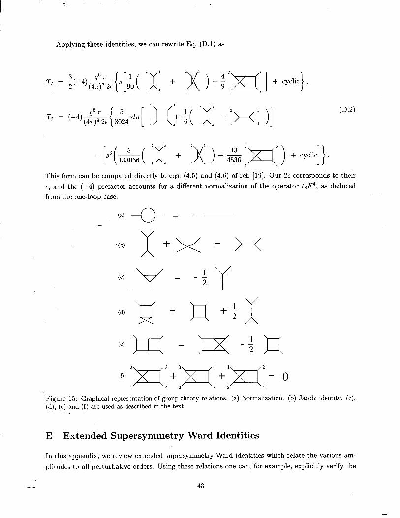
I :
Applying these identities, we can rewrite Eq. (D.l) as
’ T7 = $4 (4$;2E
- [s3(&( :x: + :x: ) + ii&$=(:) + CY~~~C]}~ This form can be compared directly to eqs. (4.5) and (4.6) of ref. [19]. Our 2~ corresponds to their
E, and the (-4) prefactor accounts for a different normalization of the operator tgF4, as deduced
from the one-loop case.
-. (4 +-- = -
- (b) x +
Figure 15: Graphical representation of group theory relations. (a) Normalization. (b) Jacobi identity. (c), (d), (e) and (f) are used as described in the text.
E Extended Supersymmetry Ward Identities
In this appendix, we review extended supersymmetry Ward identities which relate the various am-
plitudes to all perturbative orders. Using these relations one can, for example, explicitly verify the
43
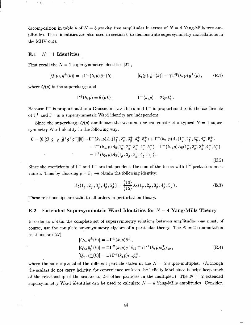
decomposition in table 4 of N = 8 gravity tree amplitudes in terms of N = 4 Yang-Mills tree am-
plitudes. These identities are also used in section 6 to demonstrate supersymmetry cancellations in
the MHV cuts.
E.1 N = 1 Identities
First recall the N = 1 supersymmetry identities [27],
[Q(d,g*(W = =v*bw ti*t(v 7 (E.1)
where Q(p) is the supercharge and
r+(k,p) = e(pk) .
Because r- is proportional to a Grassmann variable 8 and I’+ is proportional to 8, the coefficients
of I’+ and I’- in a supersymmetric Ward identity are independent.
Since the supercharge Q(p) annihilates the vacuum, one can construct a typical N = 1 super-
symmetry Ward identity in the following way:
0 = (Ol[Q,g-g-j+g+g+]lO) =r‘-(~l,p)A5(1B,2,,38,4,+,5,+) +r-(lca,p)A5(1,,2g,3B,49+,5,+)
- r-(s,p)A5(16,2s,3~,48,5~) -r+(164,P)AS(lg,29,38,48,5B)
.- - r+(k5,p)A5(l;, 2;, 3$4:,5$). 0-w
Since the coefficients of I’+ and r- are independent, the sum of the terms with l? prefactors must
vanish. Thus by choosing p = ki we obtain the following identity:
A5(1;,2;,3;,4;,5;) = =)Aj(1;,2;,3;,4,+,5,1). 0 2)
W)
These relationships are valid to all orders in perturbation theory.
E.2 Extended Supersymmetric Ward Identities for N = 4 Yang-Mills Theory
In order to obtain the complete set of supersymmetry relations between amplitudes, one must, of
course, use the complete supersymmetry algebra of a particular theory. The N = 2 commutation
relations are [27]
[&a, S*vdl = w*bwi$,
where the subscripts label the different particle states in the N = 2 super-multiplet. (Although
the scalars do not carry helicity, for convenience we keep the helicity label since it helps keep track
of the relationship of the scalars to the other particles in the multiplet.) The N = 2 extended
supersymmetry Ward identities can be used to calculate N = 4 Yang-Mills amplitudes. Consider,
44
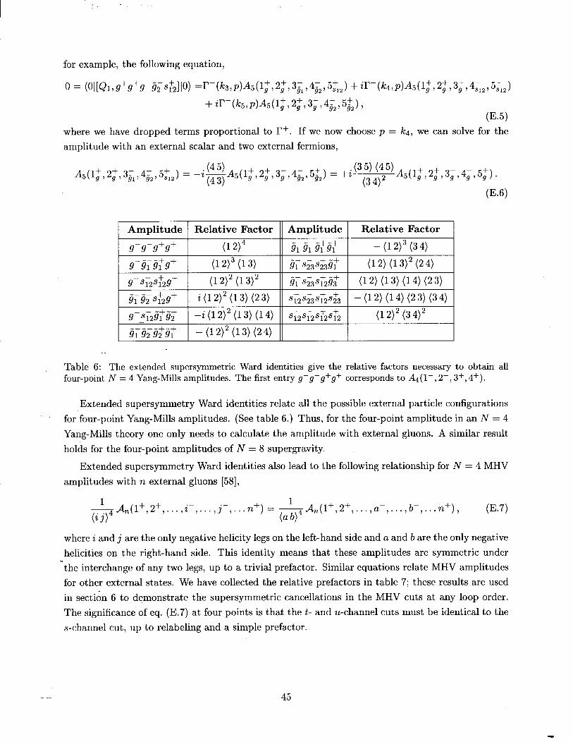
for example, the following equation,
where we have dropped terms proportional to l? + . If we now choose p = k4, we can solve for the
amplitude with an external scalar and two external fermions,
A5(1~,2~,3j1,4jr2,5~2) = -i~Ai(l:,2:,3;,4,,5~) = +i (35) (45)
(3 4)2 -4(19+:“;3;,4;,59f).
(E.6)
1 Amplitude 1 Relative Factor 11 Amplitude 1 Relative Factor 1
9-9-9+9+ (1 2j4 919xw - (12)3 (3 4)
!rim1$9+ (12)3w) 91 s;3$3$- (12) (1 3)2 (24
o&29+ (12)2 (1 3)2 51 s&i?83+ (12) (13) (14) (2 3)
iii-32 s:29+ i (12)2 (13) (23) si-2s;3st2s& - (12) (14 (2 3) (3 4
9-s12$92+ -i (12)2 (13) (14) s;2sT2s;2s;t2 (12)2 (3 4)2 ---I--+-+ 91 Q2 Q2 91 - (1 2)2 (13) (24)
. .
Table 6: The extended supersymmetric Ward identities give the relative factors necessary to obtain all four-point N = 4 Yang-Mills amplitudes. The first entry g-g-g+g+ corresponds to Ad(l-, 2-, 3+, 4+).
Extended supersymmetry Ward identities relate all the possible external particle configurations
for four-point Yang-Mills amplitudes. (See table 6.) Thus, for the four-point amplitude in an N = 4
Yang-Mills theory one only needs to calculate the amplitude with external gluons. A similar result
holds for the four-point amplitudes of N = 8 supergravity.
Extended supersymmetry Ward identities also lead to the following relationship for N = 4 MHV
amplitudes with n external gluons [58],
-&(1+,2+ ,..., i- ,..., j- ,... n+) = (i f)4
’ -&(1+,2+ ,..., a- ,..., b- ,... n+), (a fv4
(E.7)
where i and j are the only negative helicity legs on the left-hand side and a and b are the only negative
helicities on the right-hand side. This identity means that these amplitudes are symmetric under
-the interchange of any two legs, up to a trivial prefactor. Similar equations relate MHV amplitudes
for other external states. We have collected the relative prefactors in table 7; these results are used
in section 6 to demonstrate the supersymmetric cancellations in the MHV cuts at any loop order.
The significance of eq. (E.7) a t f our points is that the t- and u-channel cuts must be identical to the
s-channel cut, up to relabeling and a simple prefactor.
45
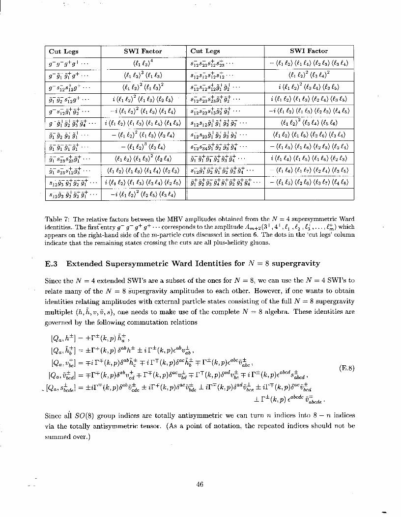
1 Cut Legs SW1 Factor
g-g-g+g+. . . g-fipj;g+ . . .
(4 e2Y 05 e2j3 (4 e3)
g-s,s;2g+. . .
ij;ij;s;2g+ . . ’
(4 e2j2 (el e3j2
i (4 e2)2 (el e3) (e2 e3)
g-q2tj;lj2+. . . 4 (e, e2)2 (e, e,) (e, e,)
g-&j2+fi3+g-. . . i (4 e2) (el e3) (4 e4) (4 e,)
I KSZS2+~~ . . 1 - (4 e2)2 (el e,) (e2 e4) [s;s1;9:s: . . . - 6 e2j3 (e3 e4) 1 lj,s;3s;3j;. ‘. 1 (6 e,) (4 e3)2 (e2 e4) Esls,s;t,~z . . I (4 e2) (6 -e3) (4 e4) (e2 e3)
I s,9,m,‘3;’ . . . 1 i (e, e,) (el e3) (e2 e4) (e2 e5) - ---+-+-+
s1292 Q2 Q2 91 . . . 4 (6 e2)2 (e, e,) (e3 e4)
Cut Legs SW1 Factor - - + +
s12s23s12s23 . ‘. - (el e2) (el e4) (e2 e3) (e3 e4)
- - + + s12s12s12s12 . . . t-e1 e2)2 (e, e4Y
- - + -+-+ s12s12s12s1 Q2 . . . i (4 e2j2 (e3 e4) (e3 e5)
- - + -+-+ S12S23S23Sl Q2 . . . i (el e2) (4 e3) (e2 e4) (e3 a,)
- - + -+-+ s12s23s13s2 Q2 . . . -i (el e2) (4 e3) t-e2 e3) (e4 e5)
- -+-+-+-+ Gp12Sl 91 g2 Q2 . . . (!l e2j2 (e3 e4) (e5 e6)
- - s,s,&wdg~~ ‘. (al e2) (el e5) (e2 e6) (e3 e4)
- - I s,s,i$&$d . . - (el e5) (el e6) (e2 e3) (e2 e4)
---+-+-+-+-+ 91 91 91 Q2 Q3 Q4 . ’ ’ i (& e4) & t5) (cl e6) (!2 f3)
- -+-+-+-+-+-+ s1291 92 91 Q2 Q3 Q4 . - (!l e6) (el e7) (e2 e4) @3 e5)
j~&j$&j$j$j$j~. . . - (& e5) (e2 e6) (e3 e7) (e4 e8)
Table 7: The relative factors between the MHV amplitudes obtained from the N = 4 supersymmetric Ward identities. The first-entry g- g- g+ g+ . . . corresponds to the amplitude Am+2 (3+, 4+, f?; , CT, e;, . . . , !k) which appears on the right-hand side of the m-particle cuts discussed in section 6. The dots in the ‘cut legs’ column indicate that the remaining states crossing the cuts are all plus-helicity gluons.
E.3 Extended Supersymmetric Ward Identities for N = 8 supergravity
Since the N = 4 extended SWI’s are a subset of the ones for N = 8, we can use the N = 4 SWI’s to
relate many of the N = 8 supergravity amplitudes to each other. However, if one wants to obtain
identities relating amplitudes with external particle states consisting of the full N = 8 super-gravity
multiplet (h, h, ZJ, v”, s), one needs to make use of the complete N = 8 algebra. These identities are
governed by the following commutation relations
(E.8)
Since ail SO(8) group indices are totally antisymmetric we can turn n indices into 8 - n indices
via the totally antisymmetric tensor. (As a point of notation, the repeated indices should not be
summed over.)
46

I
As an example of an N = 8 supergravity Ward identity consider
0 =(0 1 [Ql, h+h+h-i&s&,, ilo) = -r-(Ic3,p)~5(lh+,2~,3~114~2341 5+ 81234 >
+ + ir-(~4,p)~5(17t,2~,3~,4~1234,5s1234 ) + ir-(~5,d~5(lh+, 2ft, 3;,4;2347 5&,,),
(E.9)
which after choosing p = Icg yields the following supergravity relationships,
&(1;,2,+,3,,4,:5$) = iE M5(1Jt,2h+,3;,4,,5$) = i (45) (3 5j3
(3 4)4 IG(l:, 2,$, 3;,4h, 5;).
(E.lO)
Table 8 summarizes the relations between the five-point trees necessary for the non-singlet three-
particle cut, as deduced from the N = 8 SWI’s. The same results can be obtained from table 4, via
the KLT tree relations.
I Amplitude 1 Relative Factor 11 Amplitude I Relative Factor
h+h+h-h-h+ w8 h+h+h-h-L+
(34j7 (35)
h+h+h-v-v+ (34)6 (3 5)2 h+h+h-G-fi+ (34)5 (35)3
h+h+h-s-s+ (34)4 (3 5)4 h+h+f.-h-v+ i (3 4)6 (3 5) (4 5)
h+hFk-v-v+ (34)5 (45) (35)2 h+h+h-c-s+ i (34)4 (4 5) (3 5)3
h+h+v-v-s+ - (3 4)4 (45)2 (3 5)2 h+h+v-G--G-- -i (3 4)3 (4 5)2 (3 5)3 . .
Table 8: The N = 8 extended supersymmetry Ward identity relations between all five-point supergravity amplitudes with two positive helicity external gravitons.
Extended supersymmetry Ward identities imply that for N = 8 pure graviton amplitudes,
-&(1+,2+ ,... ,i- ,..., j- ,... n’) = ($8
1 -MMn(l+,2’ ,..., a- ,..., b- ,... n’), (a W8
(E.ll)
where i and j are the only negative helicity legs on the left-hand side and a and b are the only
negative helicities on the right-hand side. This identity is similar to eq. (E.7) for N = 4 Yang-Mills
theory, and may be proven in the same way.
References
- [l] L.D. Landau, Nucl. Phys. 13:181 (1959);
S. Mandelstam, Phys. Rev. 112:1344 (1958), 115:1741 (1959);
R.E. Cutkosky, J. Math. Phys. 1:429 (1960).
[2] H. Kawai, D.C. Lewellen and S.-H.H. Tye, Nucl. Phys. B269:l (1986).
[3] F.A. Berends, W.T. Giele and H. Kuijf, Phys. Lett. 211B:91 (1988).
[4] S.J. Parke and T.R. Taylor, Phys. Rev. Lett. 56:2459 (1986).
47
I :
[5] M.B. Green, J.H. Schwarz, and E. Witten, Superstring Theory (Cambridge University Press,
1987).
[S] M.B. Green, J.H. Schwarz and L. Brink, Nucl. Phys. B198:474 (1982).
[7] Z. Bern, D.C. Dunbar and T. Shimada, Phys. Lett. B312:277 (1993) [hep-th/9307001].
[8] D.C. Dunbar and P.S. Norridge, Nucl. Phys. B433:181 (1995) [hep-th/9408014].
[9] Z. Bern and D.A. Kosower, Nucl. Phys. B379:451 (1992).
[lo] K. Roland, Phys. Lett. 289B:148 (1992);
G. Cristofano, R. Marotta and K. Roland, Nucl. Phys. B392:345 (1993);
A. Pasquinucci and K. Roland, Nucl. Phys. B457:27 (1995) [hep-th/9508135];
P. Di Vecchia, A. Lerda, L. Magnea and R. Marotta, Phys. Lett. B351:445 (1995) [hep-
th/9502156];
P. Di Vecchia, A. Lerda, L. Magnea, R. Marotta and R. Russo, Phys. Lett. B388:65 (1996)
[hep-th/9607141]; Nucl. Phys. B469:235 (1996) [hep-th/9601143];
M.G. Schmidt and C. Schubert, Phys. Lett. B331:69 (1994) [hep-th/9403158]; Nucl. Phys.
B, Proc. Suppl. 39BC:306 (1995) [hep-ph/9408394]; in 1995 European School of High Energy
Physics: PrGeedings, eds. N. Ellis and M. Neubert (CERN, 1996) [hep-th/9611045].
[ll] Z. Bern, L. Dixon-and D.A. Kosower, Proceedings of Strings 1993, eds. M.B. Halpern, A. Sevrin
and G. Rivlis (World Scientific, Singapore, 1994) [hep-th/9311026];
Z. Bern, G. Chalmers, L. Dixon and D.A. Kosower, Phys. Rev. Lett. 72:2134 (1994) [hep-
ph/9312333].
[12] Z. Bern, L. Dixon, D.C. Dunbar and D.A. Kosower, Nucl. Phys. B425:217 (1994) [hep-
ph/9403226].
[13] Z. Bern, L. Dixon, D.C. Dunbar and D.A. Kosower, Nucl. Phys. B435:59 (1995) [hep-
ph/9409265].
[14] D.C. Dunbar and P.S. Norridge, Class. Quant. Grav. 14:351 (1997) [hep-th/9512084];
P.S. Norridge, Phys.Lett.B387:701 (1996) [hep-th/9606067].
[15] J.S. Rozowsky, preprint hep-ph/9709423.
[16] Z. Bern, L. Dixon and D.A. Kosower, Ann. Rev. Nucl. Part. Sci. 46:109 (1996) [hep-ph/9602280].
[17] Z. Bern, J.S. Rozowsky and B. Yan, Phys. Lett. B401:273 (1997) [hep-ph/9702424].
[18] Z. Bern, L. Dixon and D.A. Kosower, Nucl. Phys. B513:3 (1998), [hep-ph/9708239].
[19] N. Marcus and A. Sagnotti, Nucl. Phys. B256:77 (1985).
[20] G. ‘t Hooft and M. Veltman, Ann. Poincare Phys. Theor. A20:69 (1974).
[21] G. ‘t Hooft, Nucl. Phys. B62:444 (1973).
48

I
[22] S. Deser and P. van Nieuwenhuizen, Phys. Rev. D10:401,411 (1974);
S. Deser, H.-S. Tsao and P. van Nieuwenhuizen, Phys. Rev. D10:3337 (1974).
[23] R.E. Kallosh, Nucl. Phys. B78:293 (1974).
[24] P. van Nieuwenhuizen and C.C. Wu, J. Math. Phys. 18:182 (1977).
[25] M.H. Goroff and A. Sagnotti, Nucl. Phys. B266:709 (1986).
[26] A.E.M. van de Ven, Nucl. Phys. B378:309 (1992).
[27] M.T. Grisaru, H.N. Pendleton and P. van Nieuwenhuizen, Phys. Rev. D15:996 (1977);
M.T. Grisaru and H.N. Pendleton, Nucl. Phys. B124:81 (1977);
S.J. Parke and T. Taylor, Phys. Lett. 157B:81 (1985).
[28] M.T. Grisaru, P. van Nieuwenhuizen, and J.A.M. Vermaseren, Phys. Rev. Lett. 37:1662 (1976).
[29] M.T. Grisaru, Phys. Lett. 66B:75 (1977);
E.T. Tomboulis, Phys. Lett. B67:417 (1977).
[30] I. Robinson, unpublished;
L. Bel, Acad- Sci. Paris, Comptes Rend. 247:1094 (1958) and 248:1297 (1959).
[31] S. Deser, J.H. Kay and K.S. Stelle, Phys. Rev. Lett. 38:527 (1977).
[32] R.E. Kallosh, Phys. Lett. 99B:122 (1981).
[33] P.S. Howe, K.S. Stelle amd P.K. Townsend, Nucl. Phys. B191:445 (1981).
[34] D.J. Gross and E. Witten, Nucl. Phys. B277:l (1986).
[35] P.S. Howe and K.S. Stelle, Phys. Lett. 137B:175 (1984), Int. J. Mod. Phys. A4:1871 (1989).
[36] P.S. Howe, K.S. Stelle and P.K. Townsend, Nucl. Phys. B236:125 (1984).
[37] K.S. Stelle, private communication.
[38] M.T. Grisaru and W. Siegel, Nucl. Phys. B201:292 (1982), erratum ibid. B206:496 (1982).
[39] S.J. Gates, M.T. Grisaru, M. RoEek and W. Siegel, Superspace (Benjamin/Cummings, 1983).
-[40] B.S. Dewitt, Phys. Rev. 162:1239 (1967);
M. Veltman, in Les Houches 1975, Proceedings, Methods In Field Theory (Amsterdam 1976);
S. Sannan, Phys. Rev. D34:1749 (1986).
[41] G. ‘t Hooft, Acta Universitatis Wratislavensis no. 38, 12th Winter School of Theoretical Physics
in Karpacz; Functional and Probabilistic Methods in Quantum Field Theory, Vol. 1 (1975);
B.S. Dewitt, in Quantum Gravity 11, eds. C. Isham, R. Penrose and D. Sciama (Oxford, 1981);
L.F. Abbott, Nucl. Phys. B185:189 (1981);
L.F Abbott, M.T. Grisaru and R.K. Schaeffer, Nucl. Phys. B229:372 (1983).
49
[42] Z. Bern and D.C. Dunbar, Nucl. Phys. B379:562 (1992).
[43] P. De Causmaecker, R. Gastmans, W. Troost and T.T. Wu, Phys. Lett. 105B:215 (1981), Nucl.
Phys. B206:53 (1982);
R. Kleiss and W.J. Stirling, Nucl. Phys. B262:235 (1985);
J.F. Gunion and Z. Kunszt, Phys. Lett. 161B:333 (1985);
Z. Xu, D.-H. Zhang and L. Chang, Nucl. Phys. B291:392 (1987).
[44] M. Mangano and S.J. Parke, Phys. Rep. 200:301 (1991);
L. Dixon, in Proceedings of Theoretical Advanced Study Institute in Elementary Particle Physics
(TAX 95), ed. D.E. Soper [hep-ph/9601359].
[45] J.E. Paton and H.-M. Chan, Nucl. Phys. B10:519 (1969);
F.A. Berends and W.T. Giele, Nucl. Phys. B294:700 (1987);
D.A. Kosower, B.-H. Lee and V.P. Nair, Phys. Lett. 201B:85 (1988);
M. Mangano, S. Parke and Z. Xu, Nucl. Phys. B298:653 (1988);
Z. Bern and D.A. Kosower, Nucl. Phys. B362:389 (1991).
[46] Z. Bern, L. Dixon and D.A. Kosower, Nucl. Phys. B412:751 (1994) [hep-ph/9306240].
[47] W. Siegel, Phys. Lett. 84B:193 (1979);
D.M. Capper, D.R.T. Jones and P. van Nieuwenhuizen, Nucl. Phys. B167:479 (1980). . .
[48] N.I. Ussyukina and A.I. Davydychev, Phys. Lett. 298B:363 (1993); 305B:136 (1993); 332B:159
(1994) [hep-ph/9402223]; 348B:503 (1995) [hep-ph/9412356];
D. Kreimer, Phys. Lett. B347:107 (1995) [hep-ph/9407234]; Mod. Phys. Lett. A9:1105 (1994)
[hep-ph/9407234];
A.I. Davydychev and J.B. Tausk, Phys. Rev. D53:7381 (1996) [hep-ph/9504431];
N.I. Ussyukina, preprint hep-ph/9801261.
[49] M.B. Green, M. Gutperle and P. Vanhove, Phys. Lett. B409:177 (1997) [hep-th/9706175];
J.G. Russo and A.A. Tseytlin, Nucl. Phys. B508:245 (1997) [hep-th/9707134].
[50] W.L. van Neerven, Nucl. Phys. B268:453 (1986).
[51] Z. Bern and A.G. Morgan, Nucl. Phys. B467:479 (1996) [hep-ph/9511336].
[52] A.G. Morgan, Phys. Lett. B351:249 (1995) [hep-ph/9502230];
G. Chalmers and W. Siegel, preprint hep-ph/9708251.
[53] S. Mandelstam, Nucl. Phys. B213:149 (1983).
[54] G.D. Mahlon, Phys. Rev. D49:2197 (1994) [hep-ph/9311213]; Phys. Rev. D49:4438 (1994) [hep-
ph/9312276].
[55] N. Marcus and A. Sagnotti, Nuovo Cim. 87A:l (1985).
50

[56] I.S. Gradshteyn and I.M. Ryzhik, Table of Integrals, Series, and Products (Academic Press,
London, 1980).
[57] P. CvitanoviC, Phys. Rev. D14:1536 (1976).
[58] Z. Bern, L. Dixon, D.C. Dunbar and D.A. Kosower, Phys. Lett. 394B:105 (1997) [hep-
th/9611127].
51
Recommended