
A. Murari, G. Vagliasindi, E. Arena, P. Arena, L. Fortunaand JET EFDA contributors
EFDA–JET–PR(08)45
On the Importance of ConsideringMeasurement Errors in a Fuzzy Logic
System for Scientific Applications withExamples from Nuclear Fusion

“This document is intended for publication in the open literature. It is made available on theunderstanding that it may not be further circulated and extracts or references may not be publishedprior to publication of the original when applicable, or without the consent of the Publications Officer,EFDA, Culham Science Centre, Abingdon, Oxon, OX14 3DB, UK.”
“Enquiries about Copyright and reproduction should be addressed to the Publications Officer, EFDA,Culham Science Centre, Abingdon, Oxon, OX14 3DB, UK.”

On the Importance of ConsideringMeasurement Errors in a Fuzzy LogicSystem for Scientific Applications with
Examples from Nuclear FusionA. Murari1, G. Vagliasindi2, E. Arena2, P. Arena2, L. Fortuna2
and JET EFDA contributors*
1Consorzio RFX-Associazione EURATOM ENEA per la Fusione, I-35127 Padova, Italy.2Dipartimento di Ingegneria Elettrica Elettronica e dei Sistemi-Università degli Studi di Catania,
95125 Catania, Italy* See annex of F. Romanelli et al, “Overview of JET Results”,
(Proc. 22 nd IAEA Fusion Energy Conference, Geneva, Switzerland (2008)).
Preprint of Paper to be submitted for publication inFusion Engineering and Design
JET-EFDA, Culham Science Centre, OX14 3DB, Abingdon, UK

.

1
ABSTRACT
In practically all fields of science the measurements are affected by noise, which can sometimes be
modelled with an appropriate probability distribution function. The results of the measurements are
therefore known only within a certain interval of confidence. In many cases the noise sources is
independent from the system to be studied and the quantities to be measured. In this paper, a simple
approach to handle statistical uncertainties, due to an independent noise source, in a Fuzzy Logic
System is developed. The theoretical analysis and various tests with a benchmark show how the
statistical error bars can be interpreted as an independent “axis of complexity” with respect to the
fuzzy boundaries of the membership functions. The statistical confidence intervals in the inputs
can be transferred to the output and handled separately from the system intrinsic fuzzyness. The
main advantages of this independent treatment of the measurement errors are shown in the case of
a binary classification task: the regime confinement identification in high temperature Tokamak
plasmas. Significant improvements in the correct prediction rate have been achieved with respect
to the classification performed without considering the error bars in the measurements.
1. INTRODUCTION
Fuzzy logic is a very powerful conceptual framework [1] to model complex systems, which present a
level of uncertainty too high to be managed with traditional boolean logic. After proving very successful
in a series of engineering applications [2], in recent years this form of multivariate logic has become
increasingly accepted also in the scientific domain. Its potential has become quite clear even in Magnetic
Confinement Nuclear Fusion, where it has provided very competitive results in various fields, ranging
from prediction to identification and even physical modelling and interpretation. With regard to the
first point, disruption predictors based on Fuzzy Logic have been developed using a wide database of
JET discharges [3], improving both the rate of success and the understanding of the phenomenon. In
terms of identification, the determination of the plasma confinement regime, the fact whether the
plasma is in the L or H mode of confinement [4] has been a particularly interesting application; in this
case fuzzy logic identifiers have been compared with all the other major alternatives on a Joint European
Torus (JET) database and have provided very competitive results [5]. The L-H transition has also
been analysed by generating a Fuzzy Logic System automatically on the basis of Classification Trees
built with the CART software package [6] and the resulting rules give significant intuitive understanding
of this auto-organisation process [7].
On the other hand in Nuclear Fusion, and more generally in natural sciences, the data available
is often affected by significant error bars, which have to be properly taken into account to provide
accurate confidence intervals in the derived results. These measurement uncertainties are typically
expressed in probabilistic terms and are therefore not naturally handled by the Fuzzy Logic intellectual
framework. Indeed Fuzzy Logic is a sort of sophisticated multivariate logic based on sets with
fuzzy boundaries and is therefore meant to be used to model systems, which are inherently
characterised by these fuzzy boundaries between various states or configurations. This type of

2
complexity is conceptually different from the errors induced by the measurement process, which
introduces probabilistic uncertainties in the inputs and are usually quantified in statistical terms.
Since the sources of noise can be very often assumed to be independent from the phenomena to be
investigated, in this paper it is shown that the statistical uncertainties can be handled separately
from the inherent fuzzy sets used to model the system under study. In this way the effects of the
measurement errors can be isolated and given a specific treatment, while the power and richness of
the fuzzy treatment are fully preserved. In the next section 2, the effects of the uncertainties in the
measurements on the fuzzy inference process are analysed in the case of some simple but basic
cases using a typical benchmark system found in the literature. A brute force approach, a sort of
Monte Carlo statistical calculation, is compared with some approximate theoretical treatments,
which allow reducing significantly the computational efforts but unfortunately do no provide
completely satisfactory performance. In the following section 3, the same theoretical methods to
quantify the effects of the measurement errors are applied to a classification problem in Nuclear
Fusion, the confinement regime identification in Tokamak plasmas using signals of JET database
[8]. Further developments of the approach and potential interesting new applications are then
reviewed the last section.
2. THE STATISTICAL UNCERTAINTIES DUE TO THE MEASUREMENTS AS AN
INDEPENDENT AXIS OF COMPLEXITY
In all the scientific domains the performed measurements are not perfect and they are always known
within an interval of confidence. Therefore any form of inference process must be capable of handling
this problem and produce results with associated probabilities. The main cause of uncertainty is
normally some sort of noise, considered additive to the otherwise ideal output of the measuring
devices. The real nature of this noise is not relevant for the discussions of this paper, provided it is
uncorrelated with the quantities of the system to be measured.
In the case of complex physical phenomena modelled with FLSs, the fuzzy logic inference
process must be adequately upgraded to cope with the statistical uncertainties due to the measurement
noise. To clarify this aspect, let’s take as an example the height of people. In some contexts, like for
example for the definition of a suitable diet, it can be inappropriate to divide people in the two simple
categories of tall and small (see figure 1a) and a more sophisticated classification may be required.
A possible membership function with fuzzy boundaries could be the one represented in figure
1b. This more involved membership is adopted to take into account the inherent complexity of the
problem at hand and it does not have anything to do with the uncertainties in the measurements.
Even in the case of ideal, perfect measurements of people height, a modelling with fuzzy sets could
be required. In the treatment adopted in this paper, the errors in the measurements introduce another
dimension of complexity. Not only any input belongs to various sets with a different degree of
membership, but also that degree of membership is not absolute but must be expressed by a
probability. This additional dimension in the complexity of the problem is shown pictorially in

3
figure 2, where two axes represent the traditional fuzzy boundaries between sets and the third one
the probabilistic distribution of the membership values due to the measurement errors.
The error bars in the measurements can affect the operation of a FLS in different ways depending
on the form of the membership functions and the actual values of the measurements. The three
fundamental possibilities are reported in figure 3. In certain eventualities, the uncertainty due to the
measurement noise can be such that the input remains in a flat region of the membership function
and therefore the output of the FLS is the same as if the noise was not present (case 1 of figure 3).
A second situation is encountered when the noise can bring the input in a region where the same
membership function is involved but with a different value (case 2 in figure 3).
This of course would change the output of the FLS in a way which depends on the details of mfs
and the fuzzy rules. A last alternative arises when the noise combines with the form of the mfs in
such a way as to even involve other membership functions (case 3 in figure 3), which also affects
the output of the FLS.
To illustrate the impact of the measurement errors on FLSs, a simple fuzzy system well known
in the literature has been used as a benchmark [9]. This FLS was developed to simulate the tipping
habits of customers in a restaurant. Only two quantities, the quality of food and service, are supposed
to have an influence on the customer tip, which is the output variable. The mfs of the two inputs and
the single output are shown in figure 4.
The fuzzy rules implemented are:
1. If service is poor then tip is cheap
2. If service is excellent then tip is generous
3. If service is good and food is rancid then tip is cheap
4. If service is good and food is delicious then tip is generous
5. If service is good and food is excellent then tip is generous
To confirm the effects of the input uncertainty intervals summarised in figure 3, a systematic
investigation of this simple model has been carried out. Various confidence intervals of different
amplitude have been considered first for the single inputs and then for both of them. The expected
results have been confirmed and an illustrative example is reported in figure 5. In this case an
uncertainty interval of 15 %, simulating the measurement errors, has been assumed for both inputs,
food and service. In figure 5a) the difference between the outputs of the FLS with and without the
errors on the inputs is reported. For the inputs affected by noise, the central point and the two
extremes of the error bars have been calculated with the FLS; the derived outputs have then be
averaged and the difference between this value and the one obtained by the FLS without added
noise has been calculated (and this difference is what is plotted in figure 5a). In figure 5b), the
output variances due to the errors in the input are summarised. Inspection of figure 5 confirms that
the output of the FLS is affected only when the uncertainties in the inputs induce their values to
span regions covered by different mfs or where the mfs have different values.

4
In many cases typical of the exact sciences, even if the noise cannot be reduced at will, it is very
often possible to derive detailed information about its probability distribution function. A typical
realistic assumption, for example, is for the noise to obey Gaussian statistics. In any case, this
additional information in general can help to handle the impact of the noise on the operation of a
FLS. To this end it must be remembered that, in the interpretation proposed in this paper, the
statistic of the noise remains completely independent from the fuzzy mfs and the fuzzy rules.
Therefore, if the probability of the actual inputs in their uncertainty intervals can be calculated, the
corresponding distribution of the outputs can be derived numerically. Since the FLS can be interpreted
as a nonlinear transfer function, the output calculated assuming perfect measurements in general
does not coincide with the peak of the output probability distribution function. When this is the
case, the value calculated without noise does not represent the most likely value of the output and
can therefore be misleading.
As an illustrative example, this aspect has been investigated for the case of the benchmark
previously described. For simplicity sake, the noise has been assumed to have a uniform probability
distribution within the error bars but this does not affect the quality of the results in any significant
way. For the cases discussed in the following, the two inputs, food and service, have considered
known with an uncertainty of 40%. The probability of the FLS outputs has been tested numerically.
The inputs have been scanned and for each individual value one hundred points have been selected,
within the confidence interval, and then randomly chosen with equal probability. Therefore for
each couple of inputs a statistics of ten thousand combinations has been analysed. The output
values have been determined with the FLS and compared with the single value obtained neglecting
the noise and assuming a unique, exact value for each input. In figure 6 the outputs for two different
input combinations are shown. It is clear that in general the output of the FLS without noise can be
very different from the most likely one, once the perturbation due to the noise is taken into account.
In particular, the output of the top plot in figure 6 is generated for a service value of 2 and a food
value of 1; in the case in the bottom plot of figure 6 the service and food values are 3 and 4
respectively. Analyzing figure 4, for the last set of inputs (shown in the bottom plot) the noise
produces a significant difference in the output. This discrepancy is general and has been confirmed
using different distribution functions of the noise.
The impact of the noise in the inputs is easy to quantify in the case of binary classification
problems. To this end, it has been assumed that the output value of 0.76 indicates the propensity of
the customer to give a tip; for values below this threshold the costumers do not tip and above it they
do. Again it has been assumed that the inputs are affected by an uncertainty of 40% and the same
number of one hundred test points has been chosen as in the previous case. Both inputs have integer
values in the range [1,7] and all possible combinations have been taken in account, producing a
total of 49 outputs. Now for each of the input combinations, the average of the ten thousand outputs
has been calculated to determine whether it is below or above the threshold of 0.76. This average
value has then been compared with the one obtained assuming the input to be perfectly known. The

5
difference between the decisions to tip or not for the the cases with and without noise is plotted in
figure 7.
The main problem with the statistical, brute force approach of calculating the outputs for a large
number of inputs, representing the statistical distribution of the inputs affected by noise, is linked to
the “curse of dimensionality”. The number of combinations to be calculated increases exponentially
with the complexity of the FLS and becomes unmanageable very quickly in practical applications.
An approximate but less computationally intensive treatment would be therefore very beneficial.
After investigation of various alternatives, two types of calculations have been performed. The
activation of all the rules is calculated first for three values of the inputs, the nominal one and the
maximum and minimum possible values given the error bars. Then the outputs of the FLS is
calculated in two different ways: a) by calculating the average activation of the rules first and then
determining the single output or b) by calculating the three outputs (corresponding to the three
activations) and then averaging over the three outputs. The results of these types of calculation for
the benchmark example have been compared with the previous exhaustive approach of simulating
the noise statistics with one hundred cases. The quality of these two approximations is shown in
figure 8. It must be noted that the approach of averaging the outputs seem to provide the best
approximation. On the other hand both alternatives are not completely satisfactory even for this
very simple FLS. The performance of the approximate methods is expected to degrade significantly
with the complexity of the FLS and this is confirmed by the analysis reported in next section.
The main added value of the treatment described in this section is that a probability can be
attributed to each output of the FLS. The interpretative powers of both fuzzy logic and probability
can therefore be combined. The outputs are calculated according to the rules of fuzzy logic but their
probability can also be determined on the basis of the statistics of the noise. The additional
representational power of this combined approach can be very useful in the exact sciences as
illustrated by the application to nuclear fusion described in the next section. The approach of
computing only a limited number of strategically chosen activation values of the rules must be
adopted with extreme caution because it can provide significantly distorted outputs. The relevant
result of the treatment described in this section is that a significant improvement of the classification
power of FLS can be obtained by taking into account the noise statistics as shown in the next
section for a practical case.
3. A CASE STUDY: CONFINEMENT REGIME IDENTIFICATION IN JET
The methodology described in the last section has been applied to the case of confinement regime
identification at JET. The main objective of the analysis is a typical classification problem: to
determine whether a discharge is in the L or H mode of confinement for every point in time. To this
end, a database of 53 discharges has been verified by experts at JET, who have determined specifically
the times of the L to H and H to L transitions for each discharge. The most relevant signals to be
used have been derived with exploratory analysis techniques and in particular with the CART

6
algorithm [5] within a wider class indicated by the experts. In the end, the six signals summarised
in table I have been retained for the purpose of studying the LH transition. They are the most
relevant ones for the database, whose results are presented in this paper and their information
content is estimated to be about two orders of magnitude higher than the next most important one
(the first one discarded). In order to investigate the potential of the proposed approach to treat the
error bars, a previously automatic method to generate FLSs from CART trees has been used [7]. A
series of Fuzzy classifiers of different level of complexity have been derived and their success rate
verified. A first classification has been performed without considering the measurement errors. The
FLSs have been trained with a random set of 38 discharges and then tested on the remaining ones
(not used for the training). For each FLS, the best threshold has then been determined in an empirical
way by choosing the value witch provided the best performances.
The same training procedure has then been performed taking into account the uncertainties in
the measurements. The assumed error bars are also reported in table I. Two different estimates of
the error bars have been considered to cover realistically the entire set of discharges in the database.
Within the error bars, four different values of the signals have been selected and then the combinations
of the various inputs have been randomly chosen. Given the complexity of the FLSs under test and the
number of inputs, handling more alternatives is prohibitive in terms of computational time required.
For each combination of these inputs the value of the output has been calculated. The plasma is then
assumed to be in the state of the higher probability, i.e. in the state (L or H) which is more likely on the
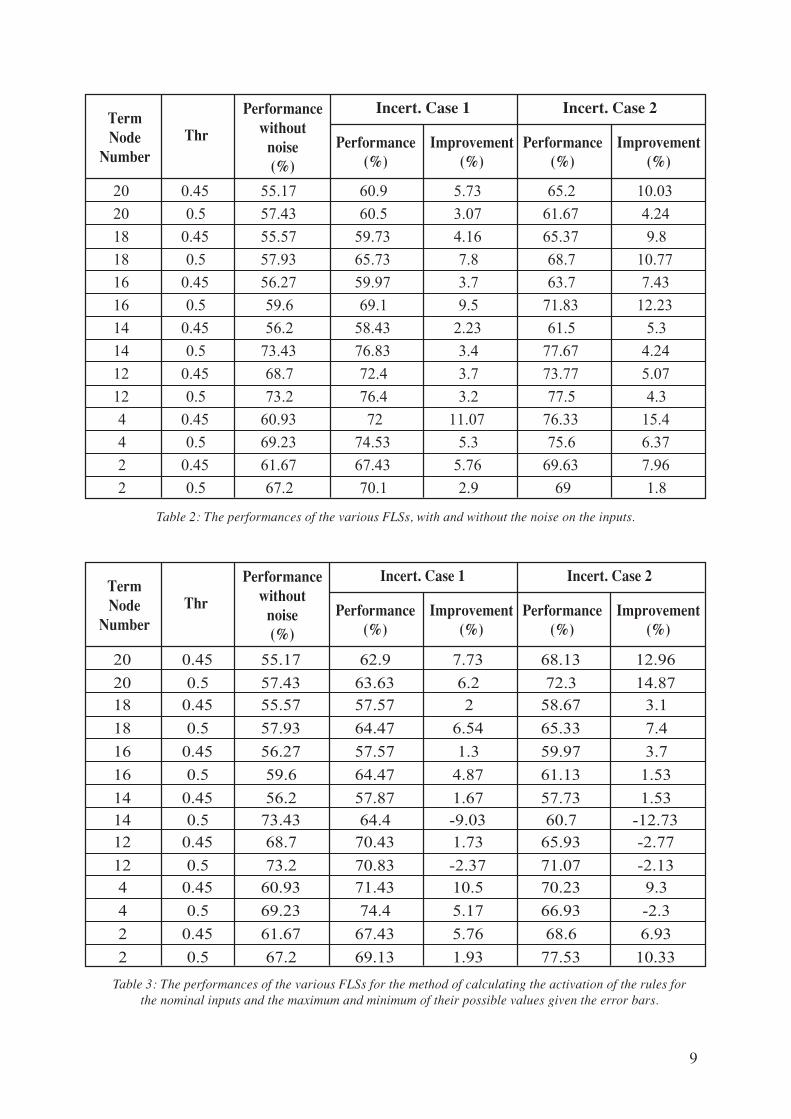
basis of the statistical distribution of the outputs. The results of the two categories of FLSs, with and
without the error bars, are compared in table II for the time interval [-100 ms, 100 ms] around the
transition. A significant improvement in the success rate is always achieved by taking into account the
most likely output instead of the simple value calculated assuming perfect measurements. In some
cases the success rate of the classifier increases of more than 12 %. Moreover the positive effect of
taking into account the statistics of the noise is significant also for the most performing FLs. It is
important to note that this interval so close to the transition is the most challenging from the point of
view of the classification and therefore it is the most vulnerable to noise.
This is confirmed by the analysis of time intervals further away from the transition time, for
which the improvement in the performance is lower because the influence of the noise is expected
to be less critical. It is also worth noticing that the improvement is in general more evident for
higher level of the assumed noise on the input signals as shown by the results of the case two. On
the other hand it has been verified that the increase in the success classification rate tends to saturate
if the assumed noise becomes unrealistically high. This suggest a possible way to determine whether
the error bars assumed are correct by increasing the noise level up to the point where the performance
of the FLS does not improve.
For some of the most performing FLs the same test has also been carried out for a higher number
of input combinations corresponding to different noise values, in order to increase the statistical
basis of the results. In general increasing the number of input values of the signals has a positive

7
effect on the classification capability of the FLs, because of course the statistical basis for the decision
becomes more solid. On the other hand, already for less than ten different values of the inputs the
computational time becomes prohibitive (several days). Therefore the same alternatives used for the
benchmark, of estimating the rule activation for the nominal values of the inputs and the points
corresponding to the limits taking into account the error bars, have also been tested on the JET database.
Unfortunately even the most performing alternative of averaging the outputs of the three values does
not provide reliable estimates, as illustrated in table III. Even if the results are in general improved,
there is a significant decrease in the success rate for the most performing FLSs. This indicates that in
general the proposed shortcuts to the full statistical analysis distort the results probably because they
do not reflect accurately enough the statistical distribution of the noise.
As a conclusion to this section, it is also worth mentioning that the proposed type of analysis,
calculating the average of the FLS outputs to take into account the confidence interval of the
measurements, is still computationally relatively manageable.
On the contrary it would be practically very difficult or even impossible to use the same approach
starting form the inputs to the CART algorithms. The CART algorithm has indeed significant
difficulties in coping efficiently with trees of the dimension required by treating statistically the
confidence intervals of the measurements already for problems with of the order of 10 inputs.
Moreover, it has been shown that applying the FLS classifier on trees generated by CART improves
the performance than using only the CART system [10]. Therefore the proposed method to derive
the statistical distribution of the outputs within the error bars of the measurements, in addition to
improving the performance of the FLS classifier, is also the only computationally practical and
simple way to attack the problem.
5. PROSPECTS OF FURTHER DEVELOPMENTS
A specific strategy has been tested to address the issue of taking into account the error bars in the
measurements used as inputs to Fuzzy Logic Systems. The approach of considering the uncertainty
of the measurements as an independent axis of complexity is conceptually sound for many real
system and provides a clear improvement in the performance of the FL classifiers when the statistic
of the noise is properly taken into account. Indeed the advantages of the adopted approach have
been tested using a JET database to classify plasma depending on their mode of confinement.
These results confirm the importance of the noise for the time interval close to the confinement
regime transition. Moreover the propose analyis can provide an independent confirmation of the
error bars estimated for the various measurements.
With regard to future developments, it would be nice to confirm the potential of the strategy for
a concrete regression problem. Also the case of a FLS with more than one output could be analysed.
Practical problems with wider error bars would probably also deserve some specific attention.
From a methodological point of view, mixtures of continuous and categorical inputs are expected
to present some additional challenges to the proposed approach. On the other hand, the prospects of

8
finding a simplified technique to avoid the statistical scan of the inputs plus noise do not look very
bright. FLSs can be very nonlinear computational processes and therefore any approximate treatment
which distorts the statistics of the noise even if lightly can have very detrimental effects on the
classification accuracy. General alternatives to the exhaustive calculation over the noisy inputs are
therefore not viable even if they can provide satisfactory results for some specific, simple cases.
REFERENCES
[1]. Zadeh L.A., “Fuzzy sets”, Infor. Control, 8, pp.338-353, 1965
[2]. Bonissone P., “Soft computing applications in prognostics and health management (PHM)”,
in Proceedings of the 8th International FLINS Conference on Computational Intelligence in
Decision and Control, Madrid, Spain September 21-24, 2008, pp. 751-756.
[3]. Murari A. et al Nucl. Fusion 48 (2008) 035010
[4]. Wagner, F. et al., Physical Review Letters 49, 1408 (1982).
[5]. Murari A. et al. IEEE Transactions on Plasma Science, Vol. 34, No. 3, June 2006
[6]. Breiman L., Friedman J.H., Olshen R.A. and Stone C.J. 1984 Classification and Regression
Trees (Belmont, CA: Wadsworth Inc.) (1993, New York: Chapman and Hall)
[7]. Vagliasindi G., Murari A., Arena P., L.Fortuna, “Automatic Derivation of a Fuzzy Logic
Classifier from Classification and Regression Trees with application to Confinement Regime
identification in Nuclear Fusion” to be submitted to IEEE Transactions on Fuzzy Systems
[8]. Andrew Y, Hawkes N.C., Martin Y.R., Crombe K., de la Luna E, Murari A, Nunes I, Sartori
R, “Access to H-mode on JET and implications for ITER” accepted for publication in Plasma
Physics and Controlled Fusion
[9]. ©1984-2007 The MathWorks, “Fuzzy Inference System”, Fuzzy Logic Toolbox of MatlabÆ.
[10]. G. Vagliasindi et al., “Comparison between CART and Fuzzy Logic for Confinement Regime
Classification at JET”, in Proceedings of the 8th International FLINS Conference on
Computational Intelligence in Decision and Control, Madrid, Spain September 21-24, 2008,
pp. 429-434.
Table 1: List of the signals used as predictors for the classification trees
Signal Name Acronym
Magneto-hydrodynamic energy Whmd (J) ± 15% ± 20%
Toroidal magnetic field BT80 (T) ± 2% ± 2%Electron temperature Te (eV) ± 10% ± 20%Beta normalised Bndiam ± 15% ± 20%X-point radial position Rxpl (m) ± 0.01% ± 0.01%X-point vertical position Zxpl (m) ± 0.01% ± 0.01%
Unit Uncert. Case 2Uncert. Case 1
9
Table 2: The performances of the various FLSs, with and without the noise on the inputs.
Table 3: The performances of the various FLSs for the method of calculating the activation of the rules forthe nominal inputs and the maximum and minimum of their possible values given the error bars.
20 0.45 55.17 60.9 5.73 65.2 10.03
20 0.5 57.43 60.5 3.07 61.67 4.24
18 0.45 55.57 59.73 4.16 65.37 9.8
18 0.5 57.93 65.73 7.8 68.7 10.77
16 0.45 56.27 59.97 3.7 63.7 7.43
16 0.5 59.6 69.1 9.5 71.83 12.23
14 0.45 56.2 58.43 2.23 61.5 5.3
14 0.5 73.43 76.83 3.4 77.67 4.24
12 0.45 68.7 72.4 3.7 73.77 5.07
12 0.5 73.2 76.4 3.2 77.5 4.3
4 0.45 60.93 72 11.07 76.33 15.4
4 0.5 69.23 74.53 5.3 75.6 6.37
2 0.45 61.67 67.43 5.76 69.63 7.96
2 0.5 67.2 70.1 2.9 69 1.8
TermNode
NumberPerformance
(%)
Performancewithout
noise(%)
Improvement(%)
Performance(%)
Improvement(%)
Thr
Incert. Case 1 Incert. Case 2
20 0.45 55.17 62.9 7.73 68.13 12.96
20 0.5 57.43 63.63 6.2 72.3 14.87
18 0.45 55.57 57.57 2 58.67 3.1
18 0.5 57.93 64.47 6.54 65.33 7.4
16 0.45 56.27 57.57 1.3 59.97 3.7
16 0.5 59.6 64.47 4.87 61.13 1.53
14 0.45 56.2 57.87 1.67 57.73 1.53
14 0.5 73.43 64.4 -9.03 60.7 -12.73
12 0.45 68.7 70.43 1.73 65.93 -2.77
12 0.5 73.2 70.83 -2.37 71.07 -2.13
4 0.45 60.93 71.43 10.5 70.23 9.3
4 0.5 69.23 74.4 5.17 66.93 -2.3
2 0.45 61.67 67.43 5.76 68.6 6.93
2 0.5 67.2 69.13 1.93 77.53 10.33
TermNode
NumberPerformance
(%)
Performancewithout
noise(%)
Improvement(%)
Performance(%)
Improvement(%)
Thr
Incert. Case 1 Incert. Case 2

10
Figure 1: a) modelling people height with crisp sets b)modelling people height with fuzzy sets without anyprovision for uncertainties in the measurements.
Figure 2: Statistical errors in the measurements of theinputs to the FLS create a second axis of uncertainty. Thex axis represents the input value, the y axis the degree ofmembership, the vertical dimension the statisticaluncertainties in the inputs and therefore the consequentprobability distribution of the membership values.
Figure 3: Three main alternatives encountered whenadding noise to the inputs of a FLS.
Figure 4: Membership functions of the inputs and theouput of the simple model for the tipping behaviour ofcustomers in restaurants: a) the input food b) the inputservice c) the output tip.
0.2
0.4
0.6
0.8
1.0
0
0
0.2
0.4
0.4
0.8
1.0
160 170 180 190 200150 210
160 170 180 190 200150 210
Deg
ree
of m
embe
rshi
p
Height (cm)
Height (cm)
Short Average Tall
JG08
.396
-1c
1
5
10
0
Input
Statisticaluncertainty
Degree of membership
JG08.396-2c
1
0
0
1
1
0
2 4 6 80 10Input
Deg
ree
of m
embe
rshi
p
JG08
.396
-3c
0.5
1.0
0.5
0.5
1.0
1.0
0
0
0.2 0.4 0.6 0.80 1.0Output variable “tip”
Cheap
DeliciousRancid
Poor Good
Excellent
Excellent
Generous
Input variable “food”
Input variable “service”JG
08.3
96-4
c

11
Figure 5: a) Error on the output of the FLS caused by theuncertainty on the inputs. The error has been defined asthe difference between the output calculated without noiseand the average of the outputs corresponding to the middleand the extremes of the confidence intervals b) Varianceof the three outputs corresponding to the middle andextremes values of the inputs with error bars.
Figure 6: Output probability distribution functions forthe benchmark comparing the cases with and withoutnoise. The red dashed line indicates the value of the outputconsidering the nominal values of the inputs (withoutnoise) while the green dashed line indicates the meanvalues of the statistical distributions. The two plots showthe outputs for two different sets of inputs (see text). Inthe case of the top graph, the difference of the outputsdue to the noise is very small and the various curves blendinto each other.
Figure 7: Top, output with binary classification; bottom,representation of the continuous output values. Thedifference in the classification of the tipping benchmarkfor the cases with and without noise can be observed.Indeed, there is a clear region of the input space wherethe most likely output for the noisy case is different fromthe one calculated without taking the noise into account.
Figure 8: Comparison of the results obtained with thetheoretical approximation of calculating a) limitedamount of activation values compared with the exhaustivecomputation of the case b).
JG08
.396
-5c
JG08
.396
-6c
JG08
.396
-7c
JG08
.396
-8c
Recommended