The 5th International Conference VŠB - Technical University of Ostrava,Czech Republic
STEELSIM 2013 10 – 12 September 2013
Numerical Study of Horizontal Centrifugal Casting of Rolls
Jan Boháček, Department of Metallurgy, Montanuniversitaet Leoben, Franz-Joseph Strasse 18, 8700 Leoben, Austria,
Abdellah Kharicha, Christian Doppler Lab for Advanced Simulation of Solidification and Melting, Dept. of
Metallurgy, Montanuniversitaet Leoben, Franz-Joseph Strasse 18, 8700 Leoben, Austria, Andreas Ludwig, Department
of Metallurgy, Montanuniversitaet Leoben, Franz-Joseph Strasse 18, 8700 Leoben, Austria, Menghuai Wu, Christian
Doppler Lab for Advanced Simulation of Solidification and Melting, Dept. of Metallurgy, Montanuniversitaet Leoben,
Franz-Joseph Strasse 18, 8700 Leoben, Austria
A numerical model was proposed to simulate casting of an outer shell of a work roll made by the horizontal centrifugal
casting (HSC) technique. The present paper is focused on the mathematical description of the average flow dynamics of
the liquid metal spreading inside the horizontally rotating mold. Later, we will target on the simulation of the whole
casting process (~35 min) which requires an extremely efficient flow algorithm. Therefore, the 2D shallow water
equations (SWE) were adopted and modified omitting the momentum in the radial direction and taking into account
forces such as the centrifugal force, the Coriolis force, the gravity force, the bed shear force, the shear force due to
turbulent effects, the wind shear force, and forces arising from the spatially variable topography. The variable
topography will later represent the solidifying liquid/solid interface. An approximate Riemann solver was developed
using the standard and corrected Roe averages. Each wave was upwinded using the Godunov’s method. The High
Resolution corrections (HR) were applied using flux limiters (MC) to keep possible sharp discontinuities in the solution.
Transonic waves leading to the expansion shocks were prevented by an extra degree of freedom giving the algorithm a
natural entropy fix. All source terms were physically bounded and well-balanced for steady states (producing non-
oscillatory solutions). The well-balancing is shown on 1D examples. The effect of forces on the shape of collapsing
parabola is shown in 1D in the circumferential direction. Steady state profiles of the liquid height under action of the
gravity are discussed for the cases with initially uniform liquid height and a hump in the topography.
1. Introduction
The horizontal centrifugal casting of rolls is a unique casting technique during which a cylindrical mold rotates around
its horizontal axis of symmetry and a melt is due to the extreme centrifugal force (~100G) pushed against the mold wall
forming the outer shell of the work roll. The schematic of the process is shown in Fig.1. The liquid metal is brought via
the filling arm inserted from one side of the mold approximately at the mold center. The mold filling takes
approximately 2 minutes and the flow rate is about 30 kg/s. During the mold filling the liquid metal adheres to the mold
and creates a ring around the circumference. As the filling proceeds, the ring expands towards the mold extremities.
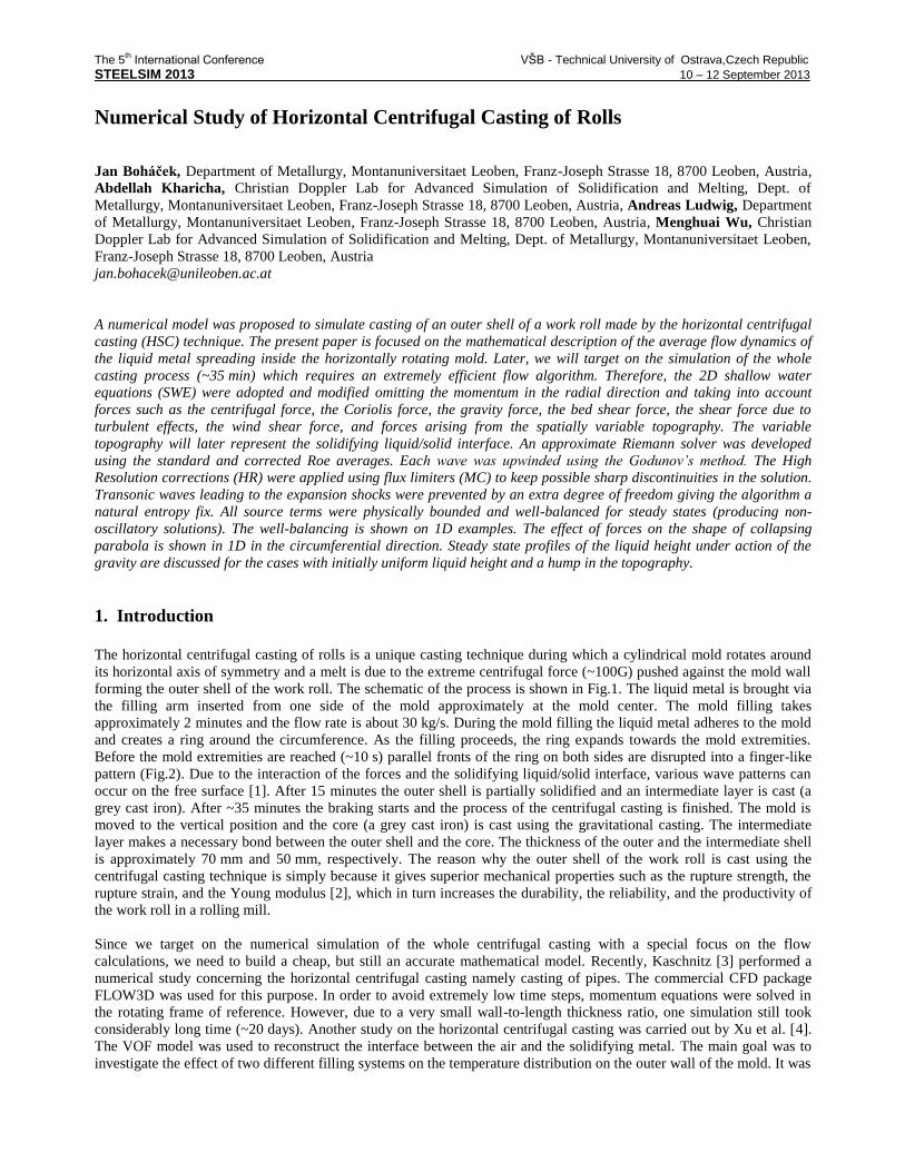
Before the mold extremities are reached (~10 s) parallel fronts of the ring on both sides are disrupted into a finger-like
pattern (Fig.2). Due to the interaction of the forces and the solidifying liquid/solid interface, various wave patterns can
occur on the free surface [1]. After 15 minutes the outer shell is partially solidified and an intermediate layer is cast (a
grey cast iron). After ~35 minutes the braking starts and the process of the centrifugal casting is finished. The mold is
moved to the vertical position and the core (a grey cast iron) is cast using the gravitational casting. The intermediate
layer makes a necessary bond between the outer shell and the core. The thickness of the outer and the intermediate shell
is approximately 70 mm and 50 mm, respectively. The reason why the outer shell of the work roll is cast using the
centrifugal casting technique is simply because it gives superior mechanical properties such as the rupture strength, the
rupture strain, and the Young modulus [2], which in turn increases the durability, the reliability, and the productivity of
the work roll in a rolling mill.
Since we target on the numerical simulation of the whole centrifugal casting with a special focus on the flow
calculations, we need to build a cheap, but still an accurate mathematical model. Recently, Kaschnitz [3] performed a
numerical study concerning the horizontal centrifugal casting namely casting of pipes. The commercial CFD package
FLOW3D was used for this purpose. In order to avoid extremely low time steps, momentum equations were solved in
the rotating frame of reference. However, due to a very small wall-to-length thickness ratio, one simulation still took
considerably long time (~20 days). Another study on the horizontal centrifugal casting was carried out by Xu et al. [4].
The VOF model was used to reconstruct the interface between the air and the solidifying metal. The main goal was to
investigate the effect of two different filling systems on the temperature distribution on the outer wall of the mold. It was
The 5th International Conference VŠB - Technical University of Ostrava,Czech Republic
STEELSIM 2013 10 – 12 September 2013
found that with the filling arm moving back and forth more uniform temperature distribution can be achieved compared
to the classical static filling. The simulation results are shown until 30 s. The solidification is not discussed in the paper.
Next, the full 3D numerical study of the full horizontal centrifugal casting was done using again the VOF model
incorporated in the commercial software STAR-CD V4 [5]. The mesh inside the mold was entirely constructed out of
rather coarse polyhedral elements, which allowed notably large time steps (~0.01 s). Only the continuity and momentum
equations were solved for the flow. Heat transfer and solidification were not discussed in the paper. Results from
simulations showed roughly how the melt is spreading during the filling, but no details are given on how the filling was
realized and whether the model could capture some free surface patterns or not.
Fig. 1 A schematic of the horizontal centrifugal casting
Several excellent experimental studies gave us a lead about the behavior of the free surface of the liquid inside a
laboratory plexiglass mold, stagnant points, and last not least some fundamental insight into the otherwise opaque
process of solidification. Recently, in-situ experiments were performed [6], in which the Succinonitrile-1 mass% water
alloy was poured in a rotating glass cell and the movement of the equiaxed crystals was observed by means of the high-
speed camera. They found that the relative path of the arbitrarily chosen equiaxed crystal associated with a fix point on
the mold oscillates and travels in the anti-rotational direction. This phenomenon can be attributed to the interaction
between the inertia of the crystal and the 3D flow influenced by effects of the gravity and vibrations. An excellent paper
[7] describing various flow regimes during the horizontal centrifuging was done to study the influence of the angular
frequency Ω and the liquid height h on waves appearing on the free surface. It was surprisingly found that with
increasing the angular frequency the free surface was more disturbed mainly due to inherent mechanical vibrations. For
low Ω the free surface formed purely cylindrical pattern. With increasing Ω a free surface pattern was passing through
the regime with helical waves, then orthogonal, and eventually “orange skin” waves. Mathematical formulas were stated
for vibrations and axial deformation of the mold to analytically investigate free surface patterns.
Fig. 2 A snapshot taken during the real casting; a side view inside the rotating mold with the liquid metal
approaching the mold extremity at ~10 s
In the present paper we focus on the development and description of a highly efficient and yet still accurate flow
algorithm solving the modified shallow water equations. In brief, the SWE were originally derived in one dimensional
form as so-called Saint-Venant equations [8] and nowadays are commonly used for modelling purposes of oceanography
and meteorology. The 2D SWE are derived from the 3D Euler equations and the continuity equation leaving out the
momentum in the vertical direction and integrating mass and momentum in the horizontal direction along the liquid
height. From the asymptotic series of the static pressure only the first term, the hydrostatic pressure is considered and
The 5th International Conference VŠB - Technical University of Ostrava,Czech Republic
STEELSIM 2013 10 – 12 September 2013
terms with higher derivatives are neglected. This as a hydrostatic condition is a leading order approximation to the static
pressure and is relevant for flows where a horizontal scale L is large compared to a characteristic height H [9]. Note that
no assumption is made about amplitudes of waves on the free surface. All the nonlinearities are retained. The original
SWE are strictly hyperbolic nonlinear PDEs.
2. Numerical model
2.1 Shallow water equations in the original form
The shallow water equations (SWE) are suitable for a numerical description of so-called gravity waves i.e. waves
formed and propagated under action of the gravitational acceleration. In 2D, the continuity and momentum equations
take the following form:
0 yxt hvhuh (1)
and
02
1 22
y
x
t huvghhuhu
02
1 22
y
xt ghhvhuvhv , (2)
where h is a liquid height, g is the gravitational acceleration, and u, v are the mass-flow averaged velocity components in
the x- and y-direction, respectively. Note that the indexes represent temporal and spatial derivatives.
2.2 Modified shallow water equations
The original SWE (eq.1-2) were modified to simulate the average flow dynamics of the liquid layer spreading inside a
horizontally rotating mold. During the observation of the real casting, the liquid melt seems to quickly pick up the speed
of the rotating mold; therefore, the choice of the rotating frame of reference is reasonably advocated. The fictitious
forces such as the centrifugal force, Fc, and the Coriolis force, FC, are thus taken into account. In addition, other forces
such as the gravity force, Fg, the bed shear force, Fµ, the shear force due to turbulent effects, Fs, and the wind shear force,
Fw, were included. Next, the SWE were derived for the variable topography b representing the actual position of the
liquid/solid interface. (Heat transfer and solidification are beyond the scope of this paper). The continuity equation stays
unmodified (eq.1), whereas the momentum equations are totally changed. The momentum equation in the axial direction
is given by:
wsgCcy
x
t FFFFFFhuvvhRhhuhu
2222
4
5
2
1 (3)
In the tangential direction the momentum equation becomes:
wsgCc
yxt FFFFFFvhRhhvhuvhv
2222
4
5
2
1 (4)
All the forces acting in the radial direction have to be decomposed into the gradient (with the x- and y-components) of
the equivalent hydrostatic pressure integrated over the liquid height h. Note, x- and y-components of the force defined in
such a way contains slopes of the liquid height h (and slopes of the topography b) in the corresponding directions. The
first term on the left hand side of eq.3 and eq.4 is an unsteady term. The second term on the left hand side of eq.3 and
eq.4 stands for the flux function written in the conservative form. It comprises the convective term, the part of the
centrifugal and Coriolis force both arising from the gradient of liquid height h. Other forces are moved on the right hand
side where each is playing a role of a source term. Both, eq.3 and eq.4 are divided by density ρ.
As mentioned in [10], we have to make certain assumptions about the velocity variation in the radial direction. The flow
is expected to be fully-hydrodynamically developed and we assume a parabolic velocity profile with a no-slip condition
on the underlying topography. Further, we assume that the liquid metal is a Newtonian fluid. From these assumptions we
can easily derive the bed shear force, which is in the x-direction given by:
h
uF
3 , (5)
The 5th International Conference VŠB - Technical University of Ostrava,Czech Republic
STEELSIM 2013 10 – 12 September 2013
where μ and ρ are a dynamic viscosity and a density, respectively. Turbulent and dispersive effects, which are
encountered during the real centrifugal casting, are included by applying a turbulent shear force given by:
uucF fs , (6)
where cf is a friction coefficient. In addition, we also consider a wind shear force, which acts on the free surface and
shears the liquid in the anti-rotational direction. It can be written in the following form:
RvRvcF ww , (7)
where Ω is the angular frequency of the rotating mold, R is the inner radius of the mold, and cw is a friction coefficient
on the free surface. The wind shear force Fw acts only in the tangential direction.
The gravity force Fg can be projected onto unit vectors in the radial and tangential direction. The radial component again
needs to be processed and finally makes a contribution to both, eq.3 and eq.4. On the other hand, the tangential
component only appears in eq.4. In the tangential direction, the gravity force Fg can be written as the following:
yyg bhtghtghF cossin , (8)
where the first term corresponds to the tangential component, whereas the second term with the slope of the free surface
stands for the radial component. A part of the centrifugal force is included in the conservative flux on the left hand side
of both momentum equations. A part of the centrifugal force resulting from the variable topography b takes the
following form:
xc RhbF 2 . (9)
Eq.9 applies to the axial direction. Analogically, the component of Fc can be determined in the tangential direction. A
similar strategy is used also for the Coriolis force. A part is included in the conservative flux and a remainder is applied
as a source term FC. Note that the Coriolis force was derived assuming a parabolic velocity profile mentioned earlier.
The Coriolis force FC in the x- and y-direction is given by:
xxC vhhvbF 2
4
52 (10)
and
yC hvbF 2 , respectively. (11)
Eq.1, eq.3, and eq.4 are modified shallow water equations for solving the average flow dynamics of a single layer
spreading over a variable topography (liquid/solid interface) in a horizontally rotating cylindrical mold. We tried to
solve this system of nonlinear PDEs using the Euler-Euler multiphase model available in the commercial CFD package
FLUENT, but the calculations were rather heavy and results were inaccurate (numerical diffusion and dispersion). For
more details see [11]. In the present paper we focus on a development of an approximate Riemann solver, which is
discussed in more details in the next chapter.
2.3 An approximate Riemann solver
The SWE (eq.1, 2) are strictly hyperbolic PDEs, which means that the Jacobian is diagonalizable with the real
eigenvalues. The SWE can be symbolically written as the following:
0,, yxt qyqBqxqAq , (12)
Where A and B are Jacobians in corresponding directions. Using the eigenvalues with the corresponding eigenvectors
the system of coupled PDEs can be transformed in a set of decoupled advection equations that can be solved separately.
The Riemann solver is used to determine fluctuations (or fluxes) through the faces of a computational cell; therefore, the
Riemann problem has to be solved for a discontinuity in each variable given by left and right state on each cell interface.
Theoretically, the true Riemann solver can be applied giving an exact solution. However, it requires solving nonlinear
equations, which increases computational costs extensively. It is rather convenient and without noticeable loss in
accuracy to use an approximate Riemann solver, which is basically based on an appropriate linearization of the Jacobian
matrix (Roe solver [12], HLLE [13], etc.). Since we update the solution using the Godunov’s splitting method, the 1D
Riemann problem is solved for each direction separately. In the present paper, we explain the 1D approximate Riemann
solver in the tangential direction. The Riemann solver in the x-direction is analogical and the derivation is easier.
Concerning the 1D Riemann solver in the tangential direction, the vector of state variables is given by:
Tjijijijijiji BHVHUHQ ,,,,,, , (13)
where i, j are cell indices, Ψ is the flux function from eq.4, and B is a height of the variable topography b. The
topography b is included in the vector of state variables (eq.13) as a stationary wave i.e. a jump in the topography leads
to a discontinuity in the solution at y=0 moving with the zero speed. This approach is used to apply source terms

The 5th International Conference VŠB - Technical University of Ostrava,Czech Republic
STEELSIM 2013 10 – 12 September 2013
including the slope of the topography and in fact, it can be used to apply any source term. The source term is upwinded
with the solution and is part of the Riemann solver. This approach is commonly advocated [14]. The fractional stepping
[15] is also an option, but it can easily produce spurious results especially when steady states are expected. It is known
that an approximate Riemann solver can accurately treat shocks and narrow rarefaction fans in either subsonic or
supersonic regime. However, it usually fails when transonic rarefaction occurs. Expansion shocks can appear and the
entropy is violated. An entropy fix has to be applied to avoid expansion shocks. We include an extra degree of freedom
by including the flux function Ψ in the vector of state variables, which leads to an overdetermined system with an extra
degree of freedom. With an appropriate choice of the wave speed the algorithm with the natural entropy fix can be
obtained. Eigenvalues of the Jacobian B are the following:
hvRhv 2
521
hvRhhv 2
5
4
5 22
v3 (14)
21
4
2
1
05 . The corresponding eigenvectors take the form:
Tur 012111
Tur 012222
Tr 000103
Tr 010004
T
RhRhuRh
r
10 2
21
2
21
25
(15)
The purpose of the Riemann solver is to decompose jumps in the state variables using the wave strengths αp for
p = 1, 2, …, 4. Such decomposition can be written as the following:
4
1
2/1,2/1,1,,
p
p
ji
p
jijiji rQQ (16)
Wave strengths αp are obtained by solving a system of linear equations:
1,, jiji QQR , (17)
where R is a matrix of eigenvectors and α is a column vector of wave strengths. In eq.14, the choice of h and v at the cell
interface is not straightforward. This is where the linearization namely the Roe linearization of the Jacobian matrix
comes into play. The Roe linearization is based on the Rankine-Hugoniot condition and finds special averages (Roe
averages) to h and v so that the left and the right states are always connected by a single wave. These special averages
are given by:
2
1,,2/1,
jijiji
hhh (18)
1,,
1,1,,,
2/1,ˆ
jiji
jijijiji
jihh
hvhvv (19)
Analogically, the Roe average 2/1,ˆ
jiu can be determined. The Roe linearization is justified by the fact that each
Riemann problem will have a large jump in at most of one wave family, in other wave families the solution will be
smooth; thus the corresponding jump will be weak. Using eq.18 and eq.19 in the original set of SWE fulfils conditions
of the Roe linearization. However, using eq.18 and eq.19 in the modified SWE (eq.1 and eq.3-4) does not. The velocity

The 5th International Conference VŠB - Technical University of Ostrava,Czech Republic
STEELSIM 2013 10 – 12 September 2013
average v in the term 5/2Ωhv in both λ
1 and λ
2 has to be corrected and this special average is given by a sum of the Roe
average 2/1,ˆ
jiv and the velocity correction as the following:
1,,1,,
,1,,1,1,,
2/1,2/1,2
ˆ
jijijiji
jijijijijiji
jijihhhh
hhhhvvvv (20)
Using this correction in the term 5/2Ωhv (eq.14) along with the Roe averages eq.18 and eq.19 fulfils conditions of the
Roe linearization. Note that the wave in the 3rd
wave family (λ3) is linearly degenerate and there is a strong analogy to
the transport of a passive tracer. The wave speed λ4 is defined as the arithmetic average of the λ
1 and λ
2, which ensures a
natural entropy fix in the case of a transonic rarefaction. The last eigenvector r5 is related to the source term containing
the slope of the topography namely the source term for the centrifugal force Fc resulting from the variable topography.
The source term part of the Riemann solver and is applied as a stationary discontinuity with the wave speed λ5 = 0. Note
that some elements in r5 require a certain scaling with respect to the wave speeds λ
1 and λ
2. This is related to the well-
balancing of steady states, which is discussed in the next chapter.
Another remark could be stated to the topic of the hyperbolicity. The original SWE are strictly hyperbolic, whereas the
modified SWE are not. In other words, at least one of the eigenvalues of the Jacobian B is not a real number. A critical
velocity vc exists and can be calculated from λ1 or λ
2 (eq.14) as the following:
Rvc 5
2. (21)
For a mold rotating in the positive direction, a typical mold radius R = 0.372 m, and an angular frequency Ω = 71 rad/s
vc becomes approximately -10.5 m/s. We see that the hyperbolicity is lost for velocity v < vc and no bound thus exists for
positive velocity v. During the real casting velocity magnitudes are expected to be in order of 0.1 m/s. Nevertheless, this
possible loss of hyperbolicity is treated by solving the original SWE with appropriate source terms, which is strictly
hyperbolic. Another trouble may arise from the fact that the Roe solver is generally not depth-positive meaning that the
Riemann solver can give a negative height h of the liquid. A simple remedy can be done using so-called Einfeldt speeds
originally suggested for the HLLE solver. The wave speeds λ1 and λ
2 are modified using the following formulas:
1
2/1,1,
11 ˆ,min jijiQ
2
2/1,,
22 ˆ,max jijiQ (22)
2.4 Well-balanced source terms
Well-balanced source terms are source terms, which exactly balance the left hand side of both, eq.3 and eq.4 in the case
when time derivatives of the state variables are zero. From the eigenvector r5 it is obvious that we need to find some
suitable average for λ1λ
2. We will show that we will eventually need two different averages for λ
1λ
2. For the sake of
brevity, we only show the derivation for the centrifugal force Fc resulting from the variable topography. The first
average 21 is derived from the momentum equation in the tangential direction omitting the local acceleration, which
can be written as the following:
y
y
RhbvhRhhv 22222
4
5
2
1
(23)
Keeping in mind 0thv , we can express eq.23 as a function of yh as the following:
yy Rhbh 221 , (24)
where 21 is an appropriate average to λ
1λ
2 in (r
5)
1 and takes the form:
1,,
1,
,
1,,2
2
1,,21
log
,min4
5
2
jiji
ji
ji
jiji
jiji
hh
h
h
hvhvhhRvv
(25)
Similarly, we can find the second average denoted by λ λ
derived from Ψy again expressed as a function of yh :
λ λ
(26)
The average λ λ
becomes:

The 5th International Conference VŠB - Technical University of Ostrava,Czech Republic
STEELSIM 2013 10 – 12 September 2013
λ λ
|vi vi - | - Ω
h -
Ωma (hvi hvi - ) (27)
Substituting hy from eq.24 for hy in eq.27 gives:
λ λ
λ λ
Ω h , (28)
which is the proper balancing of (r5)
4. Note that we do not need to balance (r
5)
2 simply because it does not appear in the
solution of the system of linear equations given by eq.17. A special care has to be taken regarding the sign of 21 and
λ λ
. Since both averages stand for an approximation to λ
1λ
2, both have to be negative for a subsonic flow and positive
for a supersonic flow. In addition, the ratio of λ λ
and
21 is always positive and greater than unity for a subsonic flow
and less than unity a supersonic flow. If any of these conditions is not satisfied, than we are dealing with a sonic point
and it is not possible to decide about the sign of the source term. In a sonic point we simply set (r5)
1 to zero and drop out
the ratio in (r5)
4.
Similar steps (eq.13-28) are followed when solving the 1D Riemann problem in the axial direction. Note that each
source term has to be limited by a certain physical bounds, which is especially required in the cases that are far from
steady states. Next, in near dry regions source terms have to be also limited in order to avoid occurrence of negative
heights in the solution.
2.5 Godunov’s explicit updating formulas with High Resolution corrections
The wave speeds λ1, λ
2, λ
3, and λ
4 with corresponding eigenvectors r
p and wave strengths α
p are used to construct
fluctuations and explicit updating formulas are used to update the solution. As mentioned earlier, we apply the
Godunov’s splitting algorithm to solve the 2D SWE i.e. for each direction we solve the 1D Riemann problem and update
the solution. (We also tested the Corner-upwind method, but we did not observe any significant differences in results on
the uniform structured orthogonal grid.) Here, we again show the updating formulas for the y-direction. The formulas for
the x-direction are analogic. The Godunov’s updating formula takes the form:
nji
nji
nji
nji QBQB
dy
dtQQ 2/1,2/1,,
1,
, (29)
where dt and dx is a time step and a grid size, respectively. The size of the time step is limited by the CFL condition. The
algorithm including all the source terms is stable for 1CFL . njiQB 2/1,
and njiQB 2/1,
are the right and left going
fluctuations, which can be calculated using the following formulas: p
jipji
p
pji
nji rQB
p
2/1,2/1,
0:
2/1,2/1,
and p
jipji
p
pji
nji rQB
p
2/1,2/1,
0:
2/1,2/1,
(30)
The Godunov’s method (eq. 29) is only first order accurate and it shows a great deal of numerical diffusion. On the other
hand, the method is not dispersive and it treats correctly the wave speeds i.e. it does not produce phase errors. The order
of accuracy can be efficiently increased by adding so-called high resolution corrections with flux limiters. A piece-wise
constant appro imation of data in the Godunov’s method is replaced by a piece-wise linear approximation. However, to
avoid overshooting especially at sharp discontinuities, the flux limiters are applied. Such scheme is still free of
numerical dispersion (or TVD scheme) and on smooth solutions is second order accurate. High resolution corrections
are applied by including correction terms in the updating formula (eq.29), which becomes:
nji
nji
nji
nji
nji
nji GG
dy
dtQBQB
dy
dtQQ 2/1,2/1,2/1,2/1,,
1,
~~
. (31)
The correction term njiG 2/1,
~ ( n
jiG 2/1,
~ ) are defined by the following formula:
pji
pji
p
pji
nji W
dy
dtG 2/1,2/1,
4
1
2/1,2/1,
~1
2
1~
, (32)
where pjiW 2/1,
~ is a limited version of p
jipjir 2/1,2/1, . In our model, we have applied the MC limiter [16].

The 5th International Conference VŠB - Technical University of Ostrava,Czech Republic
STEELSIM 2013 10 – 12 September 2013
3. Results and Discussion
All simulations were run on the uniform structured orthogonal grid with the axial and tangential dimension
corresponding to the length and the circumference of the mold, respectively. The angular frequency Ω was constant
rad/s54 . The mold was rotating in the positive direction. The time step dt was held as large as possible
corresponding to the 95.0CFL . Number of cell along the axial and tangential direction was 160 and 117.
First of all, we show results from several 1D simulations in the tangential direction i.e. around the mold circumference.
Results are presented in the form of 2D plots, in which the horizontal axis denotes the circumferential position in meters
and the vertical axis denotes a desired variable such as the liquid height h, velocity v, etc. Firstly, we demonstrate that
the algorithm is well-balanced for a steady state. A flat free surface resting upon a variable topography with a parabolic
bump should stay calm and flat forever (gravity switched off). The parabolic bump however acts as a strong source term
and if the algorithm was not well-balanced, the solution would quickly develop into artificial waves travelling on the
free surface. In Fig.3, we see the plot of the liquid height h, the topography b, and the velocity v at s60t . The free
surface obviously remains flat and velocities are negligible (<10-12
m/s) and bounded in time. Therefore, we can state
that the algorithm is well-balanced.
Fig. 3 Preserving a steady state of a liquid layer (blue) over a variable topography (red) at 60 sec
If we turn the gravity back on, we can study a steady state of the liquid layer namely the profile of the liquid height h
and the velocity v with respect to the bottom of the mold. In the flow regime when there is no recirculation of the liquid
in the radial direction, the liquid height h should be larger at the top of the mold than in the bottom. To fulfil the
continuity equation the situation should be opposite for the velocity field i.e. larger velocity in the bottom than at the top.
This will only hold when the rotating frame of reference is applicable, which means that each portion of the liquid feels
the fictitious forces. Note that this is also one of the assumptions of our numerical model. We started the simulation with
initially uniform liquid height h, zero velocity v everywhere, and the topography m0b . Due to the interaction of the
inertial forces and the gravity two counter going waves appears on the free surface. Later, these waves gradually vanish
until a steady state is reached, which is shown in Fig.4 at s60t . The position of the mold bottom is shown as a grey
dashed line. Although the liquid layer is just slightly curved, the difference in the velocity profile is enormous (~0.4m/s).
Through every revolution of the mold the liquid has to accelerate and decelerate, which exerts extreme forces on the
solidifying structure resulting in breaking of dendrite arms and an oscillatory movement of the equiaxed crystals. This
topic is discussed in details in experimental work perfomed by Esaka et. al [6]. Note that the velocity profile in Fig.4 is
typical for the horizontal centrifugal casting. No such profile can be observed in a similar process of the vertical
centrifugal casting.

The 5th International Conference VŠB - Technical University of Ostrava,Czech Republic
STEELSIM 2013 10 – 12 September 2013
Fig. 4 A steady state of a liquid layer (blue) and a velocity profile (black solid line) at 60 s; the position of
the mold bottom denoted by grey dashed line
An interesting steady state will be reached when we place a parabolic hump in the bottom of the mold, the same as the
hump in Fig.5 except that the amplitude is only 10% of the initial liquid height. In Fig.5, we can see the steady state of
both the liquid height h and velocity v again at 60 s. The free surface is disturbed by sharp discontinuities with
approximately uniform spacing. Number and amplitude of discontinuities depends on the angular frequency Ω, the mold
radius R, the initial liquid height h, and other parameters.
If we now move from 1D simulations to 2D simulations not many things will change at least concerning the case with
the topography m0b (Fig.4). The results are shown in 3D plots, in which the horizontal plane demarcates the unfolded
inner wall of the mold by the axial and circumferential position and the vertical axis denotes the liquid height h. The
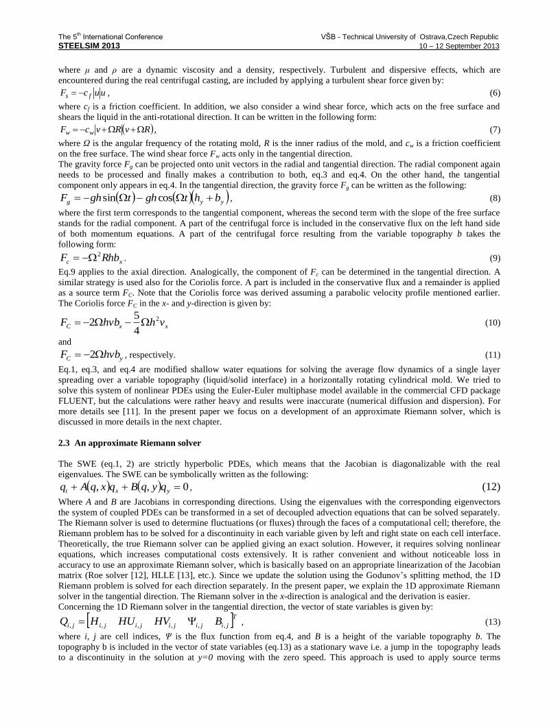
colormap is shown to pick out the variation of the liquid height h. In Fig.6, the steady state is shown for the initially flat
free surface with zero velocities (u,v) and the topography m0b . The extension to 2D obviously does not change a
steady state profile when compared to Fig.4.
Fig. 5 A steady state of a liquid layer (blue) and a velocity profile (black solid line) over a parabolic hump
at 60 s; the position of the mold bottom denoted by grey dashed line
The 5th International Conference VŠB - Technical University of Ostrava,Czech Republic
STEELSIM 2013 10 – 12 September 2013
Fig. 6 A 2D steady state of a liquid layer at 60 s; the position of the mold bottom is denoted by the blue marker
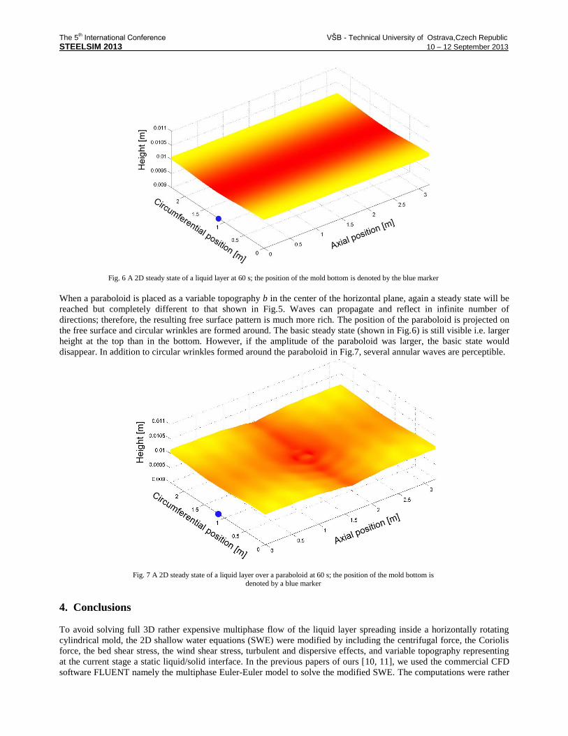
When a paraboloid is placed as a variable topography b in the center of the horizontal plane, again a steady state will be
reached but completely different to that shown in Fig.5. Waves can propagate and reflect in infinite number of
directions; therefore, the resulting free surface pattern is much more rich. The position of the paraboloid is projected on
the free surface and circular wrinkles are formed around. The basic steady state (shown in Fig.6) is still visible i.e. larger
height at the top than in the bottom. However, if the amplitude of the paraboloid was larger, the basic state would
disappear. In addition to circular wrinkles formed around the paraboloid in Fig.7, several annular waves are perceptible.
Fig. 7 A 2D steady state of a liquid layer over a paraboloid at 60 s; the position of the mold bottom is denoted by a blue marker
4. Conclusions
To avoid solving full 3D rather expensive multiphase flow of the liquid layer spreading inside a horizontally rotating
cylindrical mold, the 2D shallow water equations (SWE) were modified by including the centrifugal force, the Coriolis
force, the bed shear stress, the wind shear stress, turbulent and dispersive effects, and variable topography representing
at the current stage a static liquid/solid interface. In the previous papers of ours [10, 11], we used the commercial CFD
software FLUENT namely the multiphase Euler-Euler model to solve the modified SWE. The computations were rather

The 5th International Conference VŠB - Technical University of Ostrava,Czech Republic
STEELSIM 2013 10 – 12 September 2013
heavy and due to significant numerical diffusion and dispersion also inaccurate. Since the SWE belong to the group of
hyperbolic PDEs, we decided to change our solution strategy and developed an approximate Riemann solver. To update
the solution in time, we adopted e plicit updating formulas originally developed by Godunov. The Godunov’s method is
only first order accurate and due to the piece-wise constant approximation of data the method possesses a significant
numerical diffusion. We applied so-called high resolution corrections with flux limiters (MC limiter) so that the order of
accuracy was formally increased up to the second order. To update the solution in 2D, we used the simplest Godunov’s
splitting algorithm to keep the efficiency of the code. (We also tested the more expensive Corner-transport upwind
method with the transverse Riemann solver; however, we did not observe any significant differences in the solution.)
The Riemann solver was based on approximating the Jacobians using the Roe averages. Special correction for the
velocity related to the Coriolis force had to be applied in order to fulfill the Roe’s linearization. The algorithm is
however not depth-positive i.e. negative liquid heights can occur. To prevent negative heights, the wave speeds are
modified by means of using Einfeldt speeds originally developed for the HLLE solver. All the source terms were
included in the Riemann solver as a stationary wave. In addition, the source terms were physically bounded and well-
balanced by using the special averages of λ1λ
2, which is demonstrated in Fig.3. A certain caveat exists concerning the
sonic point, in which we are not able to decide about the sign of the special averages of λ1λ
2. A treatment of transonic
rarefactions (entropy fix) was realized by an extra wave in the Riemann solver with the speed equal to the arithmetic
average of λ1 and
λ
2.
The algorithm is fully explicit (the time step controlled by the CFL number, 1CFL ) and formally second order
accurate. The algorithm was written in MATLAB and on the same machine the serial code runs approximately 40times
faster than the former model in FLUENT. On several 1D and 2D results we show the capability of the model to capture
the steady states and briefly explain impacts of such steady states such as breaking dendrite arms, oscillatory motion of
the equiaxed crystals, or the effect of the underlying topography on the free surface pattern. We believe that with this
efficient algorithm we can later simulate the whole process of the horizontal centrifugal casting (~35 min).
Acknowledgement
Financial support by the Austrian Federal Government (in particular from the Bundesministerium fuer Verkehr,
Innovation und Technologie and the Bundesministerium fuer Wirtschaft, Familie und Jugend) and the Styrian
Provincial Government, represented by Oesterreichische Forschungsfoerderungsgesellschaft mbH and by Steirische
Wirtschaftsfoerderungsgesellschaft mbH, within the research activities of the K2 Competence Centre on "Integrated
Research in Materials, Processing and Product Engineering", operated by the Materials Center Leoben Forschung
GmbH in the framework of the Austrian COMET Competence Centre Programme, is gratefully acknowledged. This
work is also financially supported by the Eisenwerk Sulzau-Werfen R. & E. Weinberger AG.
References
[1] THORODDSEN S.T., MAHADEVAN L., 1997. Experimental study of coating flows in a partially-filled horizontally rotating cylinder,
Experiments in Fluids, 23: 1-13
[2] CHIRITA G., STEFANUSCU I., BARBOSA J., PUGA H., SOARES D., SILVA F. S., 2009. On assessment of processing variables in vertical
centrifugal casting technique, International Journal of Cast Metals Research, 382-389.
[3] KASCHNITZ E., 2012. Numerical simulation of centrifugal casting of pipes, Materials Science and Engineering, 33: 012031.
[4] XU Z., SONG N., TOL R. V., LUAN Y., LI D., 2012. Modelling of horizontal centrifugal casting of work roll, Materials Science and
Engineering, 33: 012030.
[5] KEERTHIPRASAD K. S., MURALI M. S., MUKUNDA P. G., MAJUMDAR S., 2010. Numerical Simulation and Cold Modeling experiments
on Centrifugal Casting, Metallurgical and Materials Transactions B, 42: 144-155.
[6] ESAKA H., KAWAI K., KANEKO H., SHINOZUKA K., 2012. In-Situ Observation of Horizontal Centrifugal Casting using a High-Speed
Camera, Int. Conf. MCWSP XIII published in IOP Conf. Series: Materials Science and Engineering, 33: 012041
[7] MARTINEZ G, GARNIER M, DURAND F.1987. Stirring phenomena in centrifugal casting of pipes. Applied Scientific Research, 44: 225-239.
[8] SAINT-VENANT A. J. C., 1871. Théorie du movement non permanent des eaux, avec application aux crues de rivieres et a l’introduction des
marrees dans leur lit, C. R. Acad. Sc. Paris 73: 147-154
[9] STEWART A. L., DELLAR P. J., 2010, Multilayer shallow water equations with complete Coriolis force. Part I: Derivation on a non-traditional
beta-plane, J. Fluid Mech. 651: 387-413.
[10] BOHÁČEK J., KHARICHA A., LUDWIG A., WU M., 2011. Liquid metal inside a horizontaly rotating cylinder under vibrations, Experimental Fluid Mechanics (EFM 2011), 2: 564-573.
[11] BOHÁČEK J., KHARICHA A., LUDWIG A., WU M, 2012. Shallow water model for horizontal centrifugal casting, Int. Conf. MCWSP XIII
published in IOP Conf. Series: Materials Science and Engineering, 33: 012032.

The 5th International Conference VŠB - Technical University of Ostrava,Czech Republic
STEELSIM 2013 10 – 12 September 2013
[12] LEVEQUE R. J., 2002. Finite volume methods for hyperbolic systems, Cambridge University Press, New York, 317.
[13] EINFELDT B., 1988. On Godunov-type method for gas dynamics, SIAM J. Numer. Anal., 25: 294-318.
[14] ROE P. L., 1987. Upwind differencing schemes for hyperbolic conservation laws with source terms, Lecture Notes in Math, 1270: 41–51.
[15] LEVEQUE R. J., 1998. Balancing source terms and flux gradients in high-resolution Godunov methods: The quasi-steady wave propagation algorithm. Journal of Computational Physics, 146: 346–365.
[16] VAN LEER B., 1977.Towards the ultimate conservative difference scheme IV. A new approach to numerical convection, J. Comput. Phys., 23:
276-299.
Recommended