NUMERICAL STUDY OF HEAT AND MASS
TRANSFER IN SOME INTERNAL/EXTERNAL
FLOWS
BY
MUHAMMAD FAROOQ IQBAL
CENTRE FOR ADVANCED STUDIES
IN PURE AND APPLIED MATHEMATICS
BAHAUDDIN ZAKARIYA UNIVERSITY
MULTAN, PAKISTAN.
FEBUARY 2018

NUMERICAL STUDY OF HEAT AND MASS
TRANSFER IN SOME INTERNAL/EXTERNAL
FLOWS
BY
MUHAMMAD FAROOQ IQBAL
SUPERVISED BY
PROF. DR. MUHAMMAD ASHRAF
CENTRE FOR ADVANCED STUDIES
IN PURE AND APPLIED MATHEMATICS
BAHAUDDIN ZAKARIYA UNIVERSITY
MULTAN, PAKISTAN.
FEBUARY 2018
NUMERICAL STUDY OF HEAT AND MASS TRANSFER
IN SOME INTERNAL/EXTERNAL FLOWS
A DISSERTATION SUBMITTED IN PARTIAL
FULFILLMENT OF THE REQUIREMENT
FOR THE DEGREE OF
DOCTOR OF PHILOSOPHY
IN MATHEMATICS
BY
MUHAMMAD FAROOQ IQBAL
CENTRE FOR ADVANCED STUDIES
IN PURE AND APPLIED MATHEMATICS
BAHAUDDIN ZAKARIYA UNIVERSITY
MULTAN, PAKISTAN.
FEBUARY 2018

PProophj
DEDICATEDDEDICATEDDEDICATEDDEDICATED
ToToToTo
MYMYMYMY PARENTSPARENTSPARENTSPARENTS

Certificate
It is certified that the work contained in this dissertation is original and has been
accomplished completely by MUHAMMAD FAROOQ IQBAL, under my
supervision and that, in my opinion; it is fully adequate, in scope and quality for
the degree of "DOCTOR OF PHILOSOPHY" in Mathematics.
(Supervisor)
PROF. DR. MUHAMMAD ASHRAF
Centre for Advanced Studies
in Pure and Applied Mathematics,
Bahauddin Zakariya University,
Multan.

Declaration
I hereby declare that work contained in this dissertation has not been
previously published in any form and shall not, in future, be submitted for
obtaining Ph.D. degree of any other university. All sources of information have
been acknowledged in this dissertation.
MUHAMMAD FAROOQ IQBAL

ACKNOWLEDGEMENTS
Praise and glory is to Allah, The Cherisher and The Sustainer of the worlds.
It is mere His will and grace which enabled me to accomplish this uphill task. I bow
to Him in reverence and gratitude. Peace and blessing to Hazrat Muhammad (صلى الله عليه وسلم)
who is the cause of the birth of cosmos.
Afterward, I would like to express my deep gratitude and sincere sentiments to my research supervisor and Director CASPAM PROF. Dr. Muhammad Ashraf. With great patience, he is always willing to extend valuable advice.
Thanks are also due to Dr. Kashif Ali and Dr. Shahzad Ahmad for their kind cooperation and continuous encouragement. Acknowledgement is also gratefully extended to all my honorable teachers who taught me during my studies.
I am grateful to all my friends especially Mufti Hussain Ahmad, Mr. Muhammad Ibrahim, Mr. Ahmad Hassan, Dr. Ali Ahmad, Mr. Muhammad Zubair Qureshi, Mr. Naeem Shafqat, and Dr. Muhammad Salman, whose support was essential to the realization of this work.
In the end, I am extremely grateful to my wife and children, whose continuous support was unfathomably needed for the completion of this task.
MUHAMMAD FAROOQ IQBAL

Numerical Study of Heat and Mass Transfer in Some
Internal/External Flows
Ph.D. Thesis
By
Muhammad Farooq Iqbal
Centre for Advanced Studies in Pure and Applied Mathematics
(CASPAM)
Bahauddin Zakariya University, Multan

TABLE OF CONTENTS
1 Abstract and Literature Review 1
2 Heat and Mass Transfer in Unsteady Titanium Dioxide Nano-Fluid Flow
Between Two Orthogonally Moving Porous Disks 9
2.1 Introduction 10
2.2 Mathematical Formulation 10
2.3 Numerical Solution 14
2.4 Results and Discussion 15
2.5 Conclusions 17
3 On the Combined Effect of Heat and Mass Transfer in MHD Flow of a Nano-
fluid Between Expanding / Contracting Walls of a Porous Channel
34
3.1 Introduction 35
3.2 Mathematical Formulation 35
3.3 Numerical Solution 38
3.4 Results and Discussion 40
3.5 Conclusions 42
4 On the Non –Newtonian Flow Driven by a Curved Stretching Sheet
60
4.1 Introduction 61
4.2 Mathematical Formulation 61
4.3 Numerical Solution 64
4.4 Results and Discussion 66
4.5 Conclusions 67
5 On the Suitability of Rosseland Approximation for Thermal Radiation in Flow over a Rotating Cone Embedded in Porous Media
78
5.1 Introduction 79
5.2 Mathematical Formulation 79
5.3 Numerical Solution 82
5.4 Results and Discussion 82
5.5 Conclusions 84
Possible Future Work 122
List of Publications 126
References 128

1
CHAPTER 1
ABSTRACT AND LITERATURE REVIEW

2
ABSTRACT
The purpose of this thesis is to present the numerical investigation of the heat and the mass
transfer rate in some internal/external flow problems related to the orthogonally moving disks,
expending contracting channel with porous walls, curved stretching sheet, and rotating cone.
Using the similarity variables, the governing coupled partial differential equations are converted
into non-linear ordinary differential equations which are solved numerically by using the quasi-
linearization and finite difference discretization. We have studied the momentum as well as the
heat and the mass transfer properties of the Nano-fluids and the Casson fluid. Impacts of the
relevant parameters on the behaviours of velocity, temperature, and concentration profiles are
demonstrated graphically. The skin-friction coefficient and heat and mass transfer rates are also
tabularized for different governing parameters. Further, two different models for the thermal
radiation in the flow of fluid over the rotating cone have also been compared, and some
interesting numerical results have been obtained.

3
LITERATURE REVIEW :
Flows completely bounded by the solid surfaces are called the internal flows.
Therefore internal flows include the flows through pipes, ducts, nozzles, diffusers, sudden
expansion and contractions, valves, and fittings. The external flows are the flows over the bodies
immersed in an unbounded fluid. The flows over the semi-infinite flat plate, flow around
buildings and flows over the cylinder are examples of the external flows. Depending on the
geometry, external flows can be very simple or quite complicated. Both internal and external
flows may be laminar or turbulent, compressible or incompressible.
One of the most important flows is the flow due to rotating disk. Karman [1] presented
initial work on the rotating disk flows. He applied a special substitution (known as the Von
Karman transformation) for deriving ordinary differential equations from the partial differential
equations (Navier-Stokes equations). Numerical solution for the problem of flow over a rotating
disk was presented by Cochran [2] which was further extended by Stewartson k. [3] to the flow
of fluid between both disks rotating with some angular velocities. Chapples and Stokes V. K. [4]
and Mellor G. J. et al. [5] investigated the flow of fluid when a disk was rotating and the second
one was kept static. Thermal analysis for the fluid flow through two rotating disks was presented
by Arora and Stokes [6]. Soong and Yan [7] worked on porous rotating disks. Soong C. Y. et al.
[8] studied the fluid flow among two disks rotating coaxially. Domairry and Aziz [9] studied
electrical conduction in the fluid between two plates (one permeable and the other impermeable).
Many extensions of this work may be found in the literature. For example, Joneidi et al. [10]
incorporated the magnetic field effects in the problem, whereas Hayat et al. [11] considered the
case of squeezing walls. Hussain et al. [12] examined the MHD flow of fluid and the heat
transfer in the fluid squeezed between the two disks. Time dependent squeezing MHD flow was
investigated by Shaban [13]. This work was further extended by Turkyilmazoglu [14] by
studying the shrinking of the rotating disks. In a series of papers, Gao et al. [15-18] presented
different methods for the measurement and the characterizing of low-velocity oil-water two-
phase fluid flows. Nano-fluid flows through different geometries under magnetic field or slip
effects have been studied by many researchers (for example, Makinde and Aziz [19], Bachok et
al. [20], Safaei et al.[21,22], Goodarzi et al. [23], Togun et al. [24], Hashmi et al. [25], Das et al.
[26] etc.) Majority of papers were based on constant thermo-physical properties. However, some
4
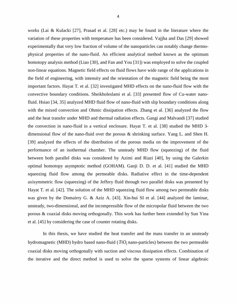
works (Lai & Kulacki [27], Prasad et al. [28] etc.) may be found in the literature where the
variation of these properties with temperature has been considered. Vajjha and Das [29] showed
experimentally that very low fraction of volume of the nanoparticles can notably change thermo-
physical properties of the nano-fluid. An efficient analytical method known as the optimum
homotopy analysis method (Liao [30], and Fan and You [31]) was employed to solve the coupled
non-linear equations. Magnetic field effects on fluid flows have wide range of the applications in
the field of engineering, with intensity and the orientation of the magnetic field being the most
important factors. Hayat T. et al. [32] investigated MHD effects on the nano-fluid flow with the
convective boundary conditions. Sheikholeslami et al. [33] presented flow of Cu-water nano-
fluid. Hsiao [34, 35] analyzed MHD fluid flow of nano-fluid with slip boundary conditions along
with the mixed convection and Ohmic dissipation effects. Zhang et al. [36] analyzed the flow
and the heat transfer under MHD and thermal radiation effects. Gangi and Malvandi [37] studied
the convection in nano-fluid in a vertical enclosure. Hayat T. et al. [38] studied the MHD 3-
dimensional flow of the nano-fluid over the porous & shrinking surface. Yang L. and Shen H.
[39] analyzed the effects of the distribution of the porous media on the improvement of the
performance of an isothermal chamber. The unsteady MHD flow (squeezing) of the fluid
between both parallel disks was considered by Azimi and Riazi [40], by using the Galerkin
optimal homotopy asymptotic method (GOHAM). Ganji D. D. et al. [41] studied the MHD
squeezing fluid flow among the permeable disks. Radiative effect in the time-dependent
axisymmetric flow (squeezing) of the Jeffery fluid through two parallel disks was presented by
Hayat T. et al. [42]. The solution of the MHD squeezing fluid flow among two permeable disks
was given by the Domairry G. & Aziz A. [43]. Xin-hui SI et al. [44] analyzed the laminar,
unsteady, two-dimensional, and the incompressible flow of the micropolar fluid between the two
porous & coaxial disks moving orthogonally. This work has further been extended by Sun Yina
et al. [45] by considering the case of counter rotating disks.
In this thesis, we have studied the heat transfer and the mass transfer in an unsteady
hydromagnetic (MHD) hydro based nano-fluid ( 2TiO nano-particles) between the two permeable
coaxial disks moving orthogonally with suction and viscous dissipation effects. Combination of
the iterative and the direct method is used to solve the sparse systems of linear algebraic

5
equations arising from the finite difference (FD) discretization of the quasi-linearized self similar
ODEs. The numerical results have been physically interpreted in chapter no. 2 of the thesis.
Study of the combined forced convection and the free convection fluid flow through the
two heated parallel vertical walls in the porous medium along with the viscous dissipation effect,
the walls are heated asymmetrically and the symmetrically, has been presented by Ingham D. B.
et al. [46]. Makinde and Mhone [47] examined the magnetohydrodynamic oscillatory flow
through the channel filled with the porous medium. Mehmood and Ali [48] studied the effect of
slip condition on the free convective oscillatory flow through the vertical channel with the
temperature (periodic) distribution. Makinde and Beg [49] devoted their study to investigate the
inherent irreversibility and thermal stability in a chemically reactive flow through the channel
with isothermal walls. Ajibade and Jha [50] investigated the effects of the suction and the
injection on the oscillatory flow through the parallel plates. In [51, 52], the problem was
extended to study the heat generation/absorption and time dependent boundary condition
(respectively). Umavathi [53] employed the Darcy-Brinkman–Forchheimer model to discuss the
natural convection fluid flow in the channel (vertical) filled with the porous medium.
Srinivasacharya and Kaladhar [54] studied the chemically reacting couple stress fluid in the
channel along with the Soret and the Dufour effects. Garg B. P. et al. [55] analyzed the influence
of Hall current in magneto-hydrodynamic viscoelastic fluid in the porous channel. Further,
several investigators made significant contributions in peristalsis under different assumptions
(for example, Kothandapani and Srinivas [56], Gnaneswara et al. [57], Ali et al. [58], Sarkar et
al. [59], Mekheimer and Abd Elmaboud [60]). Laminar and incompressible natural convective
transport inside vertical channel with porous medium has been considered by Kaladhar et al.
[61]. Falade et al. [62] investigated the effect of the suction and injection on the unsteady
oscillatory fluid flow through the channel (vertical) with the non-uniform wall temperature.
Manipulation of the heat convection of the copper particles in the blood has been considered
peristaltically, two phase model of the fluid flow is used in the channel with insulating walls
[63].
Motivated from above studies, the flow in the parallel-plate channel has been considered
in chapter no. 3 of the thesis where we have investigated the laminar flow of nano-fluid in the
channel (porous) with expanding & contracting walls via a similarity transformation. We have

6
observed that the permeability Reynolds number enhances both of the heat transfer rate and the
shear stress when the porous walls of the channel are expanding, on the other hand the viscous
dissipation always boosts the heat transfer rate at the walls, irrespective of movement of the
walls.
Fluid flow and the heat transfer analysis over the stretching surface has gained a special
focus of recent researchers and engineers on account of its considerable applications in the
engineering and industrial processes (particularly, in the production of polymer films or thin
films, in the glass fiber and production of the paper, food manufacturing, drawing of the plastic
thin films and the wires, films of the liquid in the process of condensation, the growing of
crystal, the manufacturing and extraction of the polymer and the rubber sheets etc). Flow due to
stretching of the surface was first examined by Crane L. J. [64]. Subsequently, the fluid flow
problems due to stretching surfaces under the diverse configurations have been studied by
numerous researchers. Magnetohydrodynamic boundary layer flow of the Casson fluid over the
exponentially porous shrinking sheet has been considered by Nadeem S. et al. [65]. Ali et al. [66]
analyzed the heat transfer of MHD boundary layer flow of Casson fluid. Influence of the
chemical reaction on MHD flow of the Casson nano-fluid caused by nonlinearly stretching sheet,
immersed in the porous medium, under the radiative effect and the convective boundary
condition, were studied numerically by Imran and Shafie [67]. Analysis of the rate of transfer
heat was carried out, by Abbas et al. [68], for stretching flow over the curved surface under two
thermal conditions, namely, the prescribed surface temperature (PST) and the prescribed heat
flux (PHF). Further, two-dimensional flow of non-Newtonian MHD flow of Casson fluid has
been considered by Veena et al. [69], for both PST & PHF. Some references may be found in the
scientific literature where study of the flow of viscous fluid and the heat transfer rate is done,
under the effect of applied H-field over the sheet which is curved and stretching. The Bi-
dimensional .boundary layer fluid flow of the electrically .conducting micropolar fluid, subject to
the transversely applied magnetic field, over the stretching curved sheet has been studied by
Naveed et al. [70]. The study has been further extended by the same authors (please see [71]) to
study the effect of the nano nature of the fluid. The exothermic-endothermic reaction impacts on
the MHD flow of the viscous fluid over the curved (stretching) surface were presented by Imtiaz
et al. [72].

7
Above mentioned studies motivated us to numerically study the problem of casson fluid
flow due to the curved stretching sheet, in chapter 4 of the thesis, under the action of transverse
magnetic field. Physical features of the problem in terms of the local Nusselt number, coefficient
of the skin-friction, flow velocity and thermal profiles are discussed through tables and graphs.
Thermal radiation has turn out to be a main branch of the engineering sciences and a very
important part of various applications in chemical, environmental, mechanical, solar power and
aerospace engineering. Thermal transport through radiations is much important in modern
industries for the design of efficient equipments, missiles, satellites, aircrafts, nuclear power
plants, gas turbines and the space vehicles or the various propulsion devices. Due to its useful
applications, the thermal radiation problem has fascinated several researchers during the last
three decades (some references are [73-86]). Radiation effects on boundary layer flow alongside
a symmetric wedge were studied by Mukhopadhyay [87], for the fluid viscosity varying linearly
with temperature. It was concluded that, with the increase of temperature-dependent fluid
viscosity parameter, the velocity of fluid was raised up to the cross-over point, and after that, the
velocity was found to decrease but the temperature kept on increasing. Further, flow separation
could be controlled due to variable fluid viscosity. Radiative effects on the thermal boundary
layer fluid flow induced by the stretching sheet immersed in an incompressible and the
micropolar fluid with the constant temperature on the surface, has been studied by Ishak [88].
It was observed that the rate of heat transfer at the surface reduces due to the radiative
effects. Flow and the heat transfer of the viscous nano-fluid over the nonlinearly stretching sheet,
with the radiation and variable temperature of the wall, were studied by Fekry et al. [89]. It was
noted that rise in the parameter of the thermal radiation and the nonlinear stretching sheet yielded
a reduction in the fluid temperature, which led to an increase in the heat transfer rate at the sheet.
Thermal radiation effects on heat and mass transfer past a moving vertical cylinder have been
discussed by Gnaneswara [90]. At minute values of the radiation parameter, the flow velocity
and temperature increased sharply near the surface of the cylinder, as the time passed. The mixed
convection, unsteady flow through the vertical porous plate (impulsively started) with the
thermal radiation, heat generation, chemical reaction, time dependent suction velocity, induced
magnetic field and diffusion (thermal) under the stable heat and fluxes of mass were numerically

8
analyzed by Shakhaoath et al. [91]. It was noted that the temperature decreased as the suction
and heat source were strengthened.
Effects due to the radiation parameter and the heat source/sink on the steady, two
dimensional MHD boundary layer flow of the heat and the mass transfer past a shrinking sheet
with the wall mass suction was investigated by Babu et al. [92]. Two-phase flow model of the
dusty fluid flow due to the linearly stretching of the cylinder immersed in the porous medium
under the radiation effects was studied by Manjunatha et al. [93]. Flow was described in the
terms of ‘dusty gas’ model suggested by Saffman, which treated the discrete phase and the
continuous phase as the two continua occupying the same space. Similarly, many more
references (for example, [94, 95] and the references therein) may be found in the scientific
literature where the linearized form of the radiation has been adopted. However, there are still
some references dealing with the flows in various geometries where nonlinear modeling of the
thermal radiation is used. For instance, in [96], radiation effects in the two-dimensional flow of
the second-grade fluid which is electrically conducting were examined with non-linear radiative
heat flux. Entropy generation in MHD Williamson nano-fluid over the porous shrinking sheet
has been analyzed by Bhatti et al. [97], with nonlinear thermal radiation and the chemical
reaction. The solution of the highly nonlinear coupled ordinary differential equations was
obtained by employing a combination of the Successive linearization method (SLM) and the
Chebyshev spectral collocation method. Similar nonlinear thermal radiation has been utilized in
the work [98].
After a comprehensive literature review, we have noticed that no comparison of results
has been made by using the linearized and the nonlinear forms of thermal radiation. Therefore,
the chapter 5 of the present thesis is devoted to giving a (quantitative as well as qualitative)
comparison of the results for the flow due to a rotating cone. Effect of the governing parameters
has been obtained through tables and figures.

9
CHAPTER 2
HEAT AND MASS TRANSFER IN UNSTEADY TITANIUM
DIOXIDE NANO-FLUID FLOW BETWEEN TWO
ORTHOGONALLY MOVING POROUS DISKS

10
2.1. INTRODUCTION
In this chapter, the numerical investigations of flow and mass and heat transfer in MHD
unsteady viscous flow of hydro based nano-fluid (containing nano-particles of Titanium dioxide)
between two coaxial permeable disks are presented using quasi-linearization method. The disks
are moving orthogonally. The impact of suction and viscous dissipation are taken into account.
The linear algebraic system of equations is then solved iteratively using the finite difference
discretization of self-similar ODEs.
2.2. MATHEMATICALFORMULATION
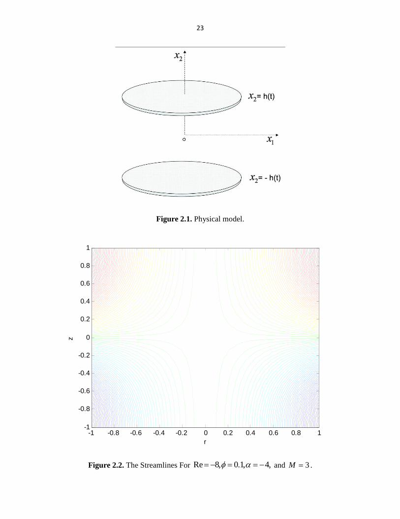
Consider the flow, heat and concentration of an incompressible and electrically conducting nano-
fluid between the two permeable coaxial disks which move orthogonally, where )(2 ta is the distance
between them, as shown in the Fig. 2.1. The assumptions regarding the flow, heat and concentration
may be summarised as
o The nano-particles 2TiO are inserted in the base fluid
o The flow is laminar and unsteady
o The fluid is of constant density and viscosity
o The disks are uniformly moving up or down at time dependent rate )(ta′
o The walls are located at a distance )(2 ta which is function of time
o cylindrical coordinate system may be chosen for this problem with origin at the centre of
both disks
o The symbols 1u and 2u represent the velocity components in the directions of 1x and 2x
respectively, where 1x represents the radius and 2x represents the z-axis
o The Joule heating, viscous dissipation and external magnetic field are taken into account
o The external applied magnetic field is acting in the perpendicular direction of the flow
o The suction through the surfaces of the disks is also taken into account
All the thermo physical properties are assumed to be constant. Water is taken as base fluid,
which is thermally stable with nano-particles and has no slip taking place among them. The
magnetic field (induced) supposed to be minor upon comparing with applied field. Magnetic

11
Reynolds number means a ratio of the product of the fluid velocity & length (characteristic) to
magnetic diffusivity. The magnetic Reynolds number, here, is utilized as a part of correlation of
magnetic force lines transportation in a fluid and seepage of those lines from the fluid. For
smaller values of the magnetic Reynolds number, the magnetic field has a tendency of relaxing
towards a purely diffusive state. No applied polarization and electric field are additionally
supposed here. Both permeable disks possess same value of the permeability. The governing
partial differential equations for the conservation of mass, momentum, heat and concentration
may be written, mathematically, as
Continuity Equation
1 1 2
1 1 2
0,u u u
x x x
∂ ∂+ + =
∂ ∂ (2.1)
r- Components of Flow Equation
22 20 11 1 1 1 1 1 1
1 2 2 2 21 2 1 1 1 2 1
1 1( ) ,e
nfnf nf
B uu u u u u u u pu u
t x x x r x x x x
συ
ρ ρ∂ ∂ ∂ ∂ ∂ ∂ ∂
+ + = + − + − −∂ ∂ ∂ ∂ ∂ ∂ ∂
(2.2)
z- Components of Flow Equation
2 22 2 2 2 2 2
1 2 2 21 2 1 1 1 2 2
1 1( ) ,nf
nf
u u u u u u pu u
t x x x x x x xυ
ρ∂ ∂ ∂ ∂ ∂ ∂ ∂
+ + = + + −∂ ∂ ∂ ∂ ∂ ∂ ∂
(2.3)
Heat Equation
( ) ( )
222 21
1 2 0 121 2 2 2
1nfnf e
p pnf nf
uT T T Tu u B u
t x x x xc c
µα σ
ρ ρ
∂∂ ∂ ∂ ∂+ + = + + ∂ ∂ ∂ ∂ ∂
, (2.4)
Concentration Equation
21 2
1 2
n n nn
C C Cu u D C
t x x
∂ ∂ ∂+ + = ∇
∂ ∂ ∂, (2.5)
Where the pressure is denoted byp , the density is denoted bynfρ and nano-fluid’s kinematics
viscosity is denoted by nfυ . Moreover, conductivity is denoted by eσ , magnetic field force is

12
denoted by , T is the temperature, nfα is the thermal diffusivity and the nC is the
concentration which may be expressed as
( ) ( ) ( )
( ) ( ) ( ) ( ) ( )
( ) ( ) ( ) ( )( )
1
2.5
1
, , 1 ,
1 , 1 , ,
2 2 2 .
nf nf snf nf nf nf
f fp nf
p p p nf fs f nf
nfs f f s s f f s
f
k
c
c c c
kk k k k k k k k
k
ρ ρυ µ ρ α ϕ ϕ
ρ ρρ
ϕ ρ ρ ϕ ρ µ µ ϕ
ϕ ϕ
−
−
−
= = = − +
+ − = = −
+ − − + + − =
(2.6)
where the densities of the solid and of the fluid, respectively, are denoted byfρ and sρ , the heat
capacitance is denoted by ( )nfpcρ and nano-fluid’s thermal conductivity is denoted by nfk [99].
The conditions on the surface of the boundary for the flow, temperature and concentration are
2 1 2 1 1( ); 0, ( ), , n nx a t u u Aa t T T C C′= − = = − = =
2 1 2 2 2( ); 0, ( ), , .n nx a t u u Aa t T T C C′= = = = = (2.7)
Where wall permeability is denoted by A. 1T and Cn1 are the temperature and concentration at the
lower disk respectively. These quantities at the upper disk are 2.T and Cn2. The temperature at the
lower disk is greater than the temperature at the upper one. Similar relation between the
concentrations at the surfaces of the two disks holds. The temperatures and concentrations are
fixed at the boundaries.
After eliminating the pressure field term from the flow equations (2.2) and (2.3) and introducing
the following similarity transformations
121 22
2 2
1 2 1 2
2, ( , ) , ( , ),
( , ) , ( , ) ,
f f
n n
n n
xxu F t u F t
a a aC C T T
t tC C T T
ξ
ν νξ ξ ξ
χ ξ θ ξ
= =− =
− −= =
− −
(2.8)
we obtain the dimensionless ODEs
2
(3 ) 2 0,nf ft
f f nf
aF F F F FF M Fξξξξ ξξ ξξξ ξξ ξξξ ξξ
υ ρα ξ
υ υ ρ+ + − − − = (2.9)
( ) ( )( )2
2.52 22 1 0,f fr c t
nf nf nf
k aF MF F P E
kξξ ξ ξ ξξ
υθ ξα θ ϕ θ
α α−
− − + + + − − =
(2.10)
0B

13
2 (2 )t fa F Dξ ξξχ ν ξα χ χ+ − = . (2.11)
With transformed B. Cs. of the form
1 Re, 0, 1, 1;
1 Re, 0, 0, 0.
at F F
and
at F F
ξ
ξ
ξ θ χ
ξ θ χ
= − = − = = =
= = = = = (2.12)
Wall expansion ratio is expressed as f
taa
υα
)(′= , the Reynolds number is expressed as
f
aAa
υ2Re
′= and the magnetic parameter is expressed as
f
e aBM
µσ 22
0= . Further, the Prandtl
number is denoted by ( )
f
fp
r k
cP
µ= , Schmidt number is denoted by DSc fν
= , the Eckert
number is denoted by ( )( )fp
c cTT
UE
21
2
−= , and the reference velocity is denoted by 1
2
fxU
a
υ= .
It is important to take a note that Equation (2.1) is identically fulfilled. This gives evidence that
the velocity and continuity equation are compatible and, therefore, signifies the motion of the
fluid.
Further, if we use the transformationRe
Ff = and keeping in view the work of [100] with α
being constant, we obtain ( )f f ξ= , ( )χ χ ξ= , ( )θ θ ξ= , 0tfξξ = . Moreover, tθ as well as tχ
reduce to zero. Accordingly, we obtain the flow, heat and concentration equations given below
2Re ( 3 ) 0,nf f
f nf
f Mf ff f fξξξξ ξξ ξξξ ξξξ ξξ
υ ρα ξ
υ ρ− − + + = (2.13)
( ) ( )( )2.52 2 22Re Re 1 0,f fr c
nf nf
kf P Mf f E
kξξ ξ ξ ξξ
υθ ξα θ ϕ
α−
− − + + − =
(2.14)
(2Re )Sc f ξ ξξξα χ χ− = , (2.15)
With the boundary conditions of flow heat and concentration
1 1, 0, 1,at f fξξ θ= − = − = = . 1;χ =
1at ξ = 1, 0, 0,f fξ θ= = =
. 0.χ = (2.16)
14
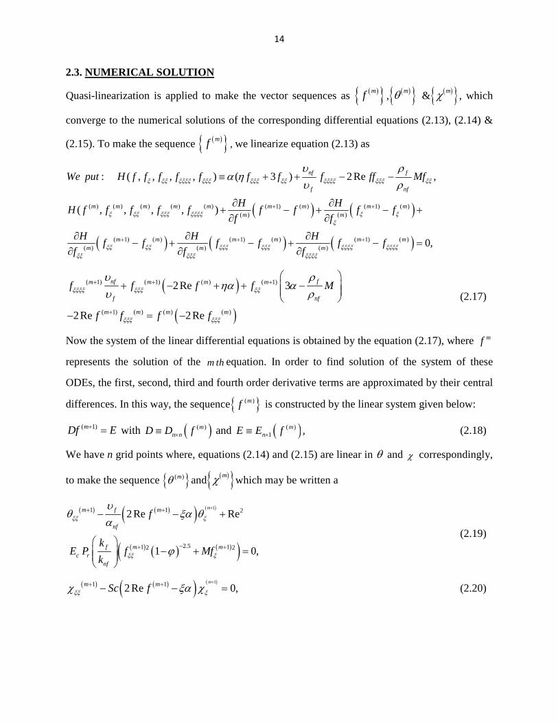
2.3. NUMERICAL SOLUTION
Quasi-linearization is applied to make the vector sequences as ( ) mf , ( ) mθ & ( ) mχ , which
converge to the numerical solutions of the corresponding differential equations (2.13), (2.14) &
(2.15). To make the sequence ( ) mf , we linearize equation (2.13) as
( ) ( )
( )
( ) ( ) ( ) ( ) ( ) ( 1) ( ) ( 1) ( )( ) ( )
( 1) ( ) ( 1)( ) ( )
: ( , , , , ) ( 3 ) 2Re ,
( , , , , )
nf f
f nf
m m m m m m m m mm m
m m mm m
We put H f f f f f f f f ff Mf
H HH f f f f f f f f f
f f
H Hf f f f
f f
ξ ξξ ξξξξ ξξξ ξξξ ξξ ξξξξ ξξξ ξξ
ξ ξξ ξξξ ξξξξ ξ ξξ
ξξ ξξ ξξξ ξξξξ ξξξ
υ ρα η
υ ρ
+ +
+ +
≡ + + − −
∂ ∂+ − + − +∂ ∂
∂ ∂− + −
∂ ∂( ) ( )( ) ( 1) ( )
( )0,m m m
m
Hf f
fξ ξξξξ ξξξξξξξξ
+∂+ − =∂
( )
( )
( 1) ( 1) ( ) ( 1)
( 1) ( ) ( ) ( )
2Re 3
2Re 2Re
nf fm m m m
f nf
m m m m
f f f f M
f f f f
ξξξξ ξξξ ξξ
ξξξ ξξξ
υ ρηα α
υ ρ+ + +
+
+ − + + −
− = −
(2.17)
Now the system of the linear differential equations is obtained by the equation (2.17), where mf
represents the solution of the m th equation. In order to find solution of the system of these
ODEs, the first, second, third and fourth order derivative terms are approximated by their central
differences. In this way, the sequence ( )mf is constructed by the linear system given below:
( 1)mDf E+ = with ( )( )mn nD D f×≡ and ( )( )
1 ,mnE E f×≡ (2.18)
We have n grid points where, equations (2.14) and (2.15) are linear in θ and χ correspondingly,
to make the sequence ( )mθ and ( ) mχ which may be written a
( ) ( )( ) ( )
( ) ( ) ( )( )
11 1 2
2.51 12 2
2Re Re
1 0,
mm f m
nf
f m mc r
nf
f
kE P f Mf
k
ξξ ξ
ξξ ξ
υθ ξα θ
α
ϕ
++ +
−+ +
− − +
− + =
(2.19)
( ) ( )( ) ( )11 12Re 0,mm mSc fξξ ξχ ξα χ++ +− − = (2.20)

15
Remarkably ( 1)mf +
, in the above frameworks of conditions, should be known. Moreover, the
central difference approximations are then substituted for derivatives. We summarize
computational method as follows:
o Make accessible the initial supposition( ) ( ) ( )000 ,, χθf fulfilling the BCs predefined in
Eq.(2.16)
o Differential equations given by Eq.(2.18) of linear system has been solved to get( )1f
o Utilize ( )1f for linear system solution emerging from the finite difference discretization
of Eqs. (2.19) and (2.20), to get ( )1θ and ( )1χ .
o The values of ( ) ( ) ( )1 1 1, &f g θ are taken to be the new initial guesses and after repeating the
method to obtain sequences ( ) ( ) ( ) , &m m mf g θ which, individually, converge to
, &f g θ ( Eqs. (2.13), (2.14) and (2.15)).
o Production of all sequences until
( ) ( ) ( ) ( ) ( ) ( ) 1 1 1 6, , 10m m m m m m
L L Lmax f f g g θ θ
∞ ∞ ∞
+ + + −− − − <
Scheme of polynomial extrapolation is also utilized to enhance the requirement of exactness of
the solution, finally.
2.4. RESULTS AND DISCUSSION
Values of the shear stress, the rate of mass and heat transfer at the surfaces of the disks
characterise the physical quantities of our concern. These quantities are related to( )1−′′f , ( )1−′χ
and ( )1−′θ . It would be sufficient to present the results only at surface of the lower disk because
of the symmetry of the problem under consideration. For present investigations the parameters
characterising the flow, heat and mass transfer are Re (Reynolds number), M (magnetic
parameter), φ (volume fraction parameter of the nano-particle), α (ratio of wall expansion), Ec
(Eckert number) and Sc (Schmidt number). Importantly, 0<α means disks are approaching
towards each other and 0>α means the disks are receding, thoughReis taken to be negative for
the suction.
16
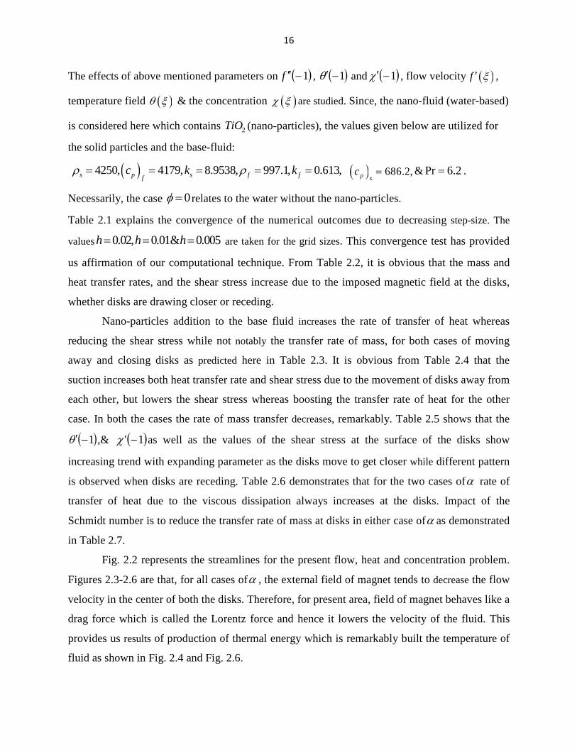
The effects of above mentioned parameters on( )1−′′f , ( )1−′θ and ( )1−′χ , flow velocity ( )f ξ′ ,
temperature field ( )θ ξ & the concentration ( )χ ξ are studied. Since, the nano-fluid (water-based)
is considered here which contains 2TiO (nano-particles), the values given below are utilized for
the solid particles and the base-fluid:
( )4250, 4179, 8.9538, 997.1, 0.613,s p s f ffc k kρ ρ= = = = = ( ) 686.2,p s
c = & 2.6Pr= .
Necessarily, the case 0=φ relates to the water without the nano-particles.
Table 2.1 explains the convergence of the numerical outcomes due to decreasing step-size. The
values 0.02, 0.01& 0.005h h h= = = are taken for the grid sizes. This convergence test has provided
us affirmation of our computational technique. From Table 2.2, it is obvious that the mass and
heat transfer rates, and the shear stress increase due to the imposed magnetic field at the disks,
whether disks are drawing closer or receding.
Nano-particles addition to the base fluid increases the rate of transfer of heat whereas
reducing the shear stress while not notably the transfer rate of mass, for both cases of moving
away and closing disks as predicted here in Table 2.3. It is obvious from Table 2.4 that the
suction increases both heat transfer rate and shear stress due to the movement of disks away from
each other, but lowers the shear stress whereas boosting the transfer rate of heat for the other
case. In both the cases the rate of mass transfer decreases, remarkably. Table 2.5 shows that the
( )1−′θ ,& ( )1' −χ as well as the values of the shear stress at the surface of the disks show
increasing trend with expanding parameter as the disks move to get closer while different pattern
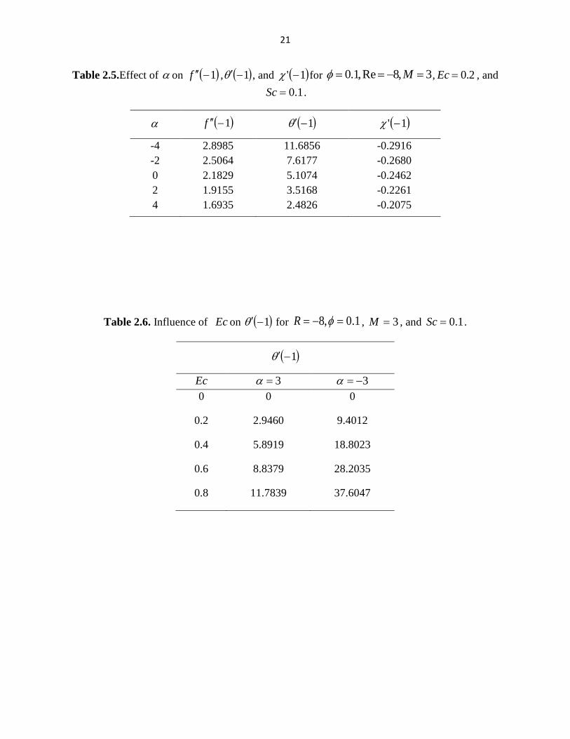
is observed when disks are receding. Table 2.6 demonstrates that for the two cases ofα rate of
transfer of heat due to the viscous dissipation always increases at the disks. Impact of the
Schmidt number is to reduce the transfer rate of mass at disks in either case ofα as demonstrated
in Table 2.7.
Fig. 2.2 represents the streamlines for the present flow, heat and concentration problem.
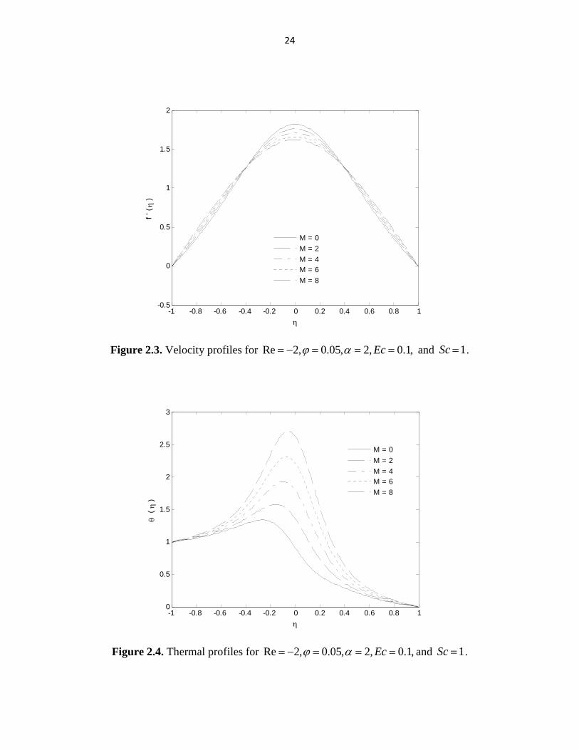
Figures 2.3-2.6 are that, for all cases ofα , the external field of magnet tends to decrease the flow
velocity in the center of both the disks. Therefore, for present area, field of magnet behaves like a
drag force which is called the Lorentz force and hence it lowers the velocity of the fluid. This
provides us results of production of thermal energy which is remarkably built the temperature of
fluid as shown in Fig. 2.4 and Fig. 2.6.
17
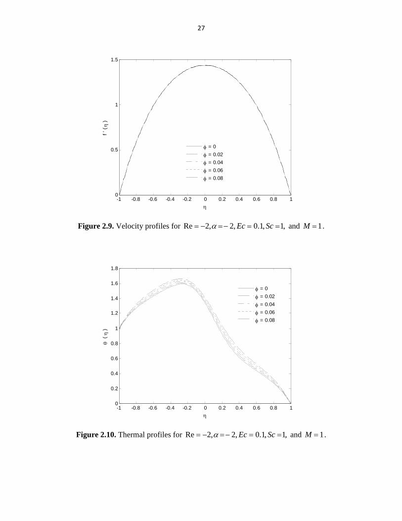
Compared to the velocity field, the impact of the nano structure of the fluid is more
prominent on the temperature distribution, regardless of the disks are approaching or moving
away shown in Figs. 2.7-2.10.
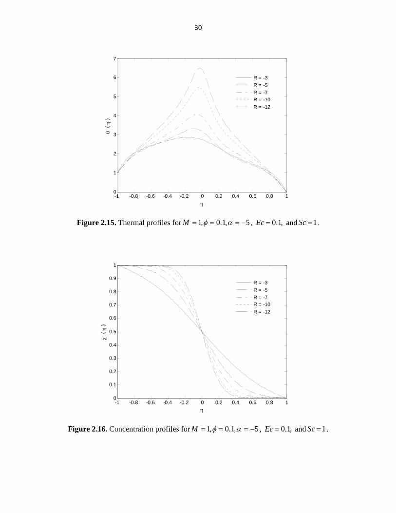
Then again, the impact of the permeability Reynolds number Re is same as that ofM for
0>α , though a contrary trend might be observed here for 0<α as shown in Figs. 2.11-2.16.
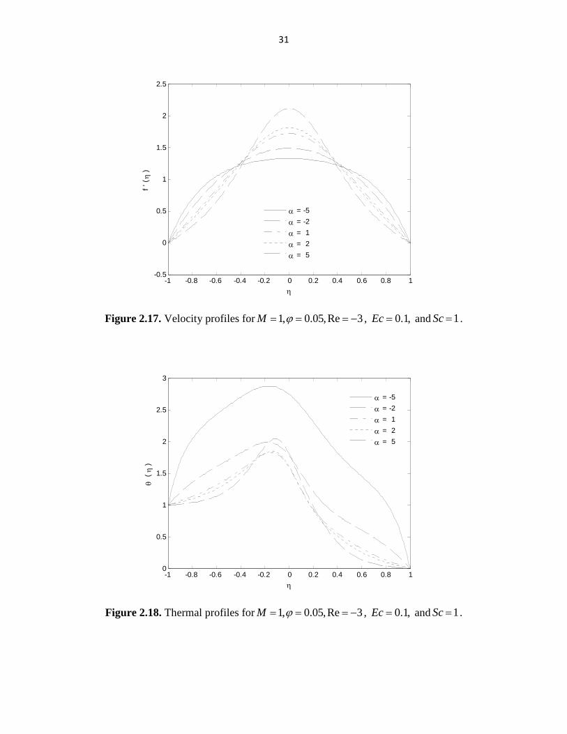
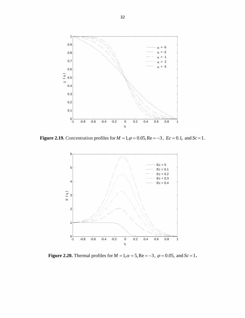
Fig. 2.17 illustrates that, as the values of α are changed from negative to positive,
velocity increases just a midst region between the disks. Fig. 2.18 uncovers that, for the disks
moving towards each other, as ratio of wall expansion α increases the temperature distribution
over the entire domain also increases. In addition, the concentration distribution increases in
lower half of the plane 0η = , while opposite trend is noted close to the upper disk as appeared in
the Fig. 2.19. In other case, the profiles of the temperature increase only in a midst of the disks.
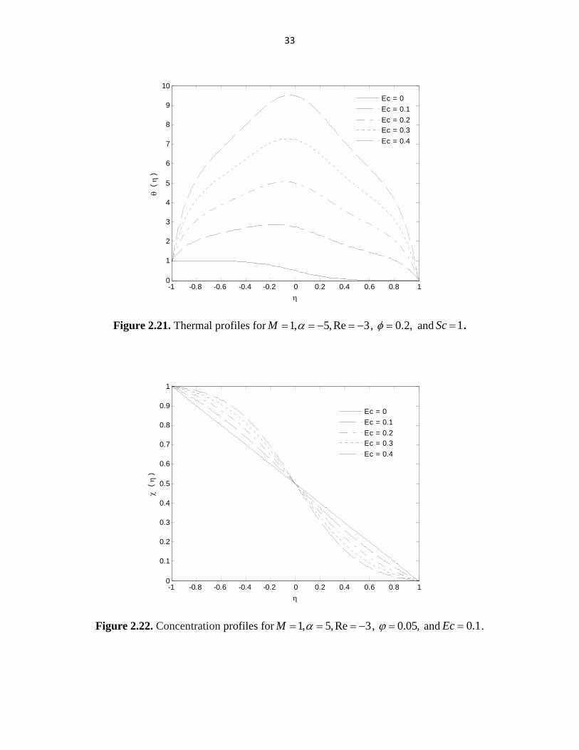
Figures 2.20 and 2.21 demonstrate that viscous dissipation significantly build temperature
dispersion over disks, apart from the disks are getting closer or receding. Finally, Fig. 2.22
demonstrates that the impact of the Schmidt number Sc on the concentration is same for both the
cases of α .
2.5. CONCLUSIONS
The numerical investigations of the problem of flow, heat and concentration of unsteady flow of
a nano-fluid with constant density and viscosity between two coaxial porous disks are presented
here taking into account the suction through the boundaries. The disks are moving orthogonally.
We want to explore that how the governing parameters, ,M Re, φ , α , ,Sc andEc affect the
flow velocity, the temperature distribution and the concentration along with the heat and mass
transfer rate.
For ( 0>α ):
1) At the surface of the disks, shear stress increases with M andRe, while contrary
impact is found for φ&α .
2) Rate of heat transfer at the disks increases with M , Re and φ , while decreases with
α .
18
3) Rate of mass transfer decreases withRe,φ , Sc and α while a contrary trend is noted
for the external magnetic field.
For ( 0<α ):
4) Shear stress at the disks increases with M and α while contrary impact is observed
for φandRe.
5) Rate of transfer of heat at the disks increases with M ,Re,α and φ .
6) Rate of transfer of mass at the disks decreases withSc ,Reand φ though an opposite
pattern is noted for α and M .

19
Table 2.1. ( )f ξ for 4,1.0,8Re −==−= αφ , 3=M , 2.0=Ec , and . 0.1Sc = .
( )f ξ
ξ 1st Grid
size
2nd Grid size
3rd Grid size
Extrapolated values
0 0.2 0.4 0.6 0.8
0 0.3018240 0.5755708 0.7971402 0.9455484
0 0.3018321 0.5755883 0.7971641 0.9455688
0 0.3018342 0.5755927 0.7971701 0.9455739
0 0.3018348 0.5755941 0.7971721 0.9455756
Table 2.2. Effect of M on ( )1−′θ , ( )1−′′f ,.and ( )1' −χ .for Re 8, 0.1ϕ=− = , 1.0=Sc and
2.0=Ec .
3=α 3−=α
M ( )1−′θ ( )1' −χ ( )1−′′f ( )1−′θ ( )1' −χ
1
2
3
4
5
1.7397
1.7695
1.7994
1.8294
1.8595
2.7556
2.8499
2.9460
3.0438
3.1435
-0.2161
-0.2163
-0.2166
-0.2169
-0.2171
2.6130
2.6530
2.6930
2.7329
2.7727
8.8637
9.1308
9.4012
9.6749
9.9518
-0.2790
-0.2793
-0.2796
-0.2799
-0.2808
Table 2.3. Effect of φ on. ( )1−′θ , ( )1−′′f and ( )1' −χ .for Re 8, 3M=− = , 1.0=Sc , 2.0=Ec
( )1−′′f

20
3=α 3−=α
( )1−′θ ( )1' −χ ( )1−′′f ( )1−′θ ( )1' −χ
0
0.02
0.04
0.06
0.08
1.8304
1.8220
1.8149
1.8088
1.8037
2.2662
2.3771
2.4996
2.6345
2.7829
-0.2169
-0.2168
-0.2167
-0.2167
-0.2166
2.7325
2.7225
2.7137
2.7059
2.6991
7.2501
7.6087
8.0003
8.4274
8.8932
-0.2799
-0.2798
-0.2797
-0.2797
-0.2796
Table 2.4. Effect of Re on ( )1−′′f , ( )1−′θ , and ( )1' −χ for ,1.0=φ ,3=M 2.0,2.6Pr == Ec ,
and 1.0=Sc .
3=α 3−=α
Re ( )1−′θ ( )1' −χ ( )1−′′f ( )1−′θ ( )1' −χ
-3 -6 -9 -12 -15
1.6163 1.7507 1.8174 1.8561 1.8813
0.7315 1.9976 3.4358 4.9428 6.4839
-0.3467 -0.2625 -0.1964 -0.1453 -0.1064
3.7274 2.9363 2.6108 2.4476 2.3517
8.7523 8.8845 9.7417 10.9532 12.3242
-0.4356 -0.3357 -0.2545 -0.1904 -0.1408
φ ( )1−′′f
( )1−′′f
21
Table 2.5.Effect of α on ( )1−′′f , ( )1−′θ , and ( )1' −χ for 3,8Re,1.0 =−== Mφ , 2.0=Ec , and
1.0=Sc .
α ( )1−′θ ( )1' −χ
-4 -2 0 2 4
2.8985 2.5064 2.1829 1.9155 1.6935
11.6856 7.6177 5.1074 3.5168 2.4826
-0.2916 -0.2680 -0.2462 -0.2261 -0.2075
Table 2.6. Influence of . Ec on ( )1−′θ for 1.0,8 =−= φR , 3=M , and 1.0=Sc .
( )1−′θ
Ec 3=α 3−=α 0
0.2
0.4
0.6
0.8
0
2.9460
5.8919
8.8379
11.7839
0
9.4012
18.8023
28.2035
37.6047
( )1−′′f

22
Table 2.7. Effect of Sc on ( )1' −χ for 1.0,8Re =−= φ , 3=M , and 2.0=Ec .
( )1' −χ
Sc 3=α 3−=α
0
0.1
0.2
0.3
0.4
-0.5000
-0.2166
-0.0841
-0.0302
-0.0103
-0.5000
-0.2796
-0.1472
-0.0738
-0.0357
23
Figure 2.1. Physical model.
Figure 2.2. The Streamlines.For ,4,1.0,8Re −==−= αφ and 3=M .
r
z
-1 -0.8 -0.6 -0.4 -0.2 0 0.2 0.4 0.6 0.8 1-1
-0.8
-0.6
-0.4
-0.2
0
0.2
0.4
0.6
0.8
1
24
Figure 2.3. Velocity profiles for Re 2, 0.05, 2, 0.1,Ecϕ α= − = = = and 1=Sc .
Figure 2.4. Thermal profiles for Re 2, 0.05, 2, 0.1,Ecϕ α= − = = = and 1=Sc .
-1 -0.8 -0.6 -0.4 -0.2 0 0.2 0.4 0.6 0.8 1-0.5
0
0.5
1
1.5
2
η
f ' (
η )
M = 0
M = 2
M = 4M = 6
M = 8
-1 -0.8 -0.6 -0.4 -0.2 0 0.2 0.4 0.6 0.8 10
0.5
1
1.5
2
2.5
3
η
θ (
η )
M = 0
M = 2
M = 4M = 6
M = 8

25
Figure 2.5. Velocity profiles forRe 2, 0.05, 2ϕ α= − = = − , ,1.0=Ec and 1=Sc .
Figure 2.6. Thermal profiles forRe 2, 0.05, 2ϕ α= − = = − , ,1.0=Ec and 1=Sc .
-1 -0.8 -0.6 -0.4 -0.2 0 0.2 0.4 0.6 0.8 10
0.5
1
1.5
η
f ' (
η )
M = 0
M = 2
M = 4M = 6
M = 8
-1 -0.8 -0.6 -0.4 -0.2 0 0.2 0.4 0.6 0.8 10
0.5
1
1.5
2
2.5
3
3.5
4
4.5
η
θ (
η )
M = 0
M = 2
M = 4M = 6
M = 8

26
Figure 2.7. Velocity profiles for ,1,1.0,2,2Re ===−= ScEcα and 1=M .
Figure 2.8. Thermal profiles for ,1,1.0,2,2Re ===−= ScEcα and 1=M .
-1 -0.8 -0.6 -0.4 -0.2 0 0.2 0.4 0.6 0.8 1-0.2
0
0.2
0.4
0.6
0.8
1
1.2
1.4
1.6
1.8
η
f ' (
η )
φ = 0
φ = 0.02
φ = 0.04
φ = 0.06
φ = 0.08
-1 -0.8 -0.6 -0.4 -0.2 0 0.2 0.4 0.6 0.8 10
0.5
1
1.5
η
θ (
η )
φ = 0
φ = 0.02
φ = 0.04
φ = 0.06
φ = 0.08
27
Figure 2.9. Velocity profiles for ,1,1.0,2,2Re ==−=−= ScEcα and 1=M .
Figure 2.10. Thermal profiles for ,1,1.0,2,2Re ==−=−= ScEcα and 1=M .
-1 -0.8 -0.6 -0.4 -0.2 0 0.2 0.4 0.6 0.8 10
0.5
1
1.5
η
f ' (
η )
φ = 0
φ = 0.02
φ = 0.04
φ = 0.06
φ = 0.08
-1 -0.8 -0.6 -0.4 -0.2 0 0.2 0.4 0.6 0.8 10
0.2
0.4
0.6
0.8
1
1.2
1.4
1.6
1.8
η
θ (
η )
φ = 0
φ = 0.02
φ = 0.04
φ = 0.06
φ = 0.08

28
Figure 2.11. Velocity profiles for 5,1.0,1 === αφM , ,1.0=Ec and 1=Sc .
Figure 2.12. Thermal profiles for the 1, 0.05, 5M ϕ α= = = , ,1.0=Ec and 1=Sc .
-1 -0.8 -0.6 -0.4 -0.2 0 0.2 0.4 0.6 0.8 1-0.5
0
0.5
1
1.5
2
2.5
η
f ' (
η )
R = -3
R = -5
R = -7R = -10
R = -12
-1 -0.8 -0.6 -0.4 -0.2 0 0.2 0.4 0.6 0.8 10
1
2
3
4
5
6
7
8
η
θ (
η )
R = -3
R = -5
R = -7R = -10
R = -12

29
Figure 2.13. Concentration profiles for 5,1.0,1 === αφM , ,1.0=Ec and 1=Sc .
Figure 2.14. Velocity profiles for 5,1.0,1 −=== αφM , ,1.0=Ec and 1=Sc .
-1 -0.8 -0.6 -0.4 -0.2 0 0.2 0.4 0.6 0.8 10
0.1
0.2
0.3
0.4
0.5
0.6
0.7
0.8
0.9
1
η
χ
( η
)
R = -3
R = -5
R = -7R = -10
R = -12
-1 -0.8 -0.6 -0.4 -0.2 0 0.2 0.4 0.6 0.8 10
0.2
0.4
0.6
0.8
1
1.2
1.4
1.6
η
f ' (
η )
R = -3
R = -5
R = -7R = -10
R = -12
30
Figure 2.15. Thermal profiles for 5,1.0,1 −=== αφM , ,1.0=Ec and 1=Sc .
Figure 2.16. Concentration profiles for 5,1.0,1 −=== αφM , ,1.0=Ec and 1=Sc .
-1 -0.8 -0.6 -0.4 -0.2 0 0.2 0.4 0.6 0.8 10
1
2
3
4
5
6
7
η
θ (
η )
R = -3
R = -5
R = -7R = -10
R = -12
-1 -0.8 -0.6 -0.4 -0.2 0 0.2 0.4 0.6 0.8 10
0.1
0.2
0.3
0.4
0.5
0.6
0.7
0.8
0.9
1
η
χ
( η
)
R = -3
R = -5
R = -7R = -10
R = -12
31
Figure 2.17. Velocity profiles for 1, 0.05,Re 3M ϕ= = = − , ,1.0=Ec and 1=Sc .
Figure 2.18. Thermal profiles for 1, 0.05,Re 3M ϕ= = = − , ,1.0=Ec and 1=Sc .
-1 -0.8 -0.6 -0.4 -0.2 0 0.2 0.4 0.6 0.8 1-0.5
0
0.5
1
1.5
2
2.5
η
f ' (
η )
α = -5
α = -2
α = 1
α = 2
α = 5
-1 -0.8 -0.6 -0.4 -0.2 0 0.2 0.4 0.6 0.8 10
0.5
1
1.5
2
2.5
3
η
θ (
η )
α = -5
α = -2
α = 1
α = 2
α = 5
32
Figure 2.19. Concentration profiles for 1, 0.05,Re 3M ϕ= = = − , ,1.0=Ec and 1=Sc .
Figure 2.20. Thermal profiles for 1, 5,Re 3M α= = = − , 0.05,ϕ = and 1=Sc .
-1 -0.8 -0.6 -0.4 -0.2 0 0.2 0.4 0.6 0.8 10
0.1
0.2
0.3
0.4
0.5
0.6
0.7
0.8
0.9
1
η
χ
( η
)
α = -5
α = -2
α = 1
α = 2
α = 5
-1 -0.8 -0.6 -0.4 -0.2 0 0.2 0.4 0.6 0.8 10
1
2
3
4
5
6
η
θ (
η )
Ec = 0
Ec = 0.1
Ec = 0.2Ec = 0.3
Ec = 0.4
33
Figure 2.21. Thermal profiles for 1, 5,Re 3M α= = − = − , ,2.0=φ and 1=Sc .
Figure 2.22. Concentration profiles for 1, 5,Re 3M α= = = − , 0.05,ϕ = and 1.0=Ec .
-1 -0.8 -0.6 -0.4 -0.2 0 0.2 0.4 0.6 0.8 10
1
2
3
4
5
6
7
8
9
10
η
θ (
η )
Ec = 0
Ec = 0.1
Ec = 0.2Ec = 0.3
Ec = 0.4
-1 -0.8 -0.6 -0.4 -0.2 0 0.2 0.4 0.6 0.8 10
0.1
0.2
0.3
0.4
0.5
0.6
0.7
0.8
0.9
1
η
χ
( η
)
Ec = 0
Ec = 0.1
Ec = 0.2Ec = 0.3
Ec = 0.4

34
CHAPTER 3
ON THE COMBINED EFFECT OF HEAT AND MASS
TRANSFER IN MHD FLOW OF A NANO-FLUID
BETWEEN EXPANDING / CONTRACTING WALLS OF
A POROUS CHANNEL
35
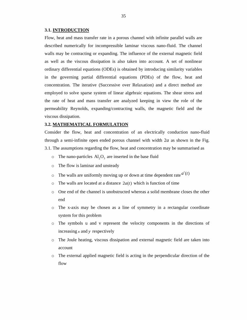
3.1. INTRODUCTION
Flow, heat and mass transfer rate in a porous channel with infinite parallel walls are
described numerically for incompressible laminar viscous nano-fluid. The channel
walls may be contracting or expanding. The influence of the external magnetic field
as well as the viscous dissipation is also taken into account. A set of nonlinear
ordinary differential equations (ODEs) is obtained by introducing similarity variables
in the governing partial differential equations (PDEs) of the flow, heat and
concentration. The iterative (Successive over Relaxation) and a direct method are
employed to solve sparse system of linear algebraic equations. The shear stress and
the rate of heat and mass transfer are analyzed keeping in view the role of the
permeability Reynolds, expanding/contracting walls, the magnetic field and the
viscous dissipation.
3.2. MATHEMATICAL FORMULATION
Consider the flow, heat and concentration of an electrically conduction nano-fluid
through a semi-infinite open ended porous channel with width 2a as shown in the Fig.
3.1. The assumptions regarding the flow, heat and concentration may be summarised as
o The nano-particles 2 3Al O are inserted in the base fluid
o The flow is laminar and unsteady
o The walls are uniformly moving up or down at time dependent rate )(ta′
o The walls are located at a distance )(2 ta which is function of time
o One end of the channel is unobstructed whereas a solid membrane closes the other
end
o The x-axis may be chosen as a line of symmetry in a rectangular coordinate
system for this problem
o The symbols u and v represent the velocity components in the directions of
increasingx andy respectively
o The Joule heating, viscous dissipation and external magnetic field are taken into
account
o The external applied magnetic field is acting in the perpendicular direction of the
flow

36
The equations of the continuity, momentum (in both the directions), heat and
concentration with constant density and viscosity for the problem under consideration
take the following mathematical form
0u u
x y
∂ ∂+ =
∂ ∂, (3.1)
( )2
021 nfnf
nf nf
B uu u u pu v u
t x y x
συ
ρ ρ∂ ∂ ∂ ∂+ + = − + ∇ −
∂ ∂ ∂ ∂, (3.2)
( )21nf
nf
v v v pu v v
t x y yυ
ρ∂ ∂ ∂ ∂+ + = − + ∇
∂ ∂ ∂ ∂, (3.3)
2 202 2( ) ( )
( ) ( )nf nf
nfp nf p nf
B uT T T uu v T
t x y c y c
µ σα
ρ ρ∂ ∂ ∂ ∂
+ + = ∇ + +∂ ∂ ∂ ∂
, (3.4)
( )2C C Cu v D C
t x y
∂ ∂ ∂+ + = ∇
∂ ∂ ∂ (3.5)
The symbol p indicates the pressure field, nfρ represents the constant density of the nano-
fluid, nfυ shows the kinematics viscosity, nfα signifies the thermal diffusivity and acts
as the strength of the magnetic field. Further, T , C and D are the temperature,
concentration and effective diffusion coefficient respectively.
Following the research contributions [101-102], we have:
( )
( )
( ) ( )( ) ( ) ( ) ( )( ) ( )
( )
2.5
3( 1)
1 , ,1( 2) ( 1)
1 , ,
2 21 , ,
2
,
s
nf f fnf
s sf
f f
nfnf f s nf
nf
s f f snfp p ps f nf
f s f f s
nfnf
p nf
k k k kkc c c
k k k k k
k
c
σφ
σ σ µµ
σ σσ ϕφσ σ
µρ ϕ ρ ϕρ υ
ρ
ϕϕ ρ ϕ ρ ρ
ϕ
αρ
− = + =−+ − −
= − + =
+ − − + − = = + + −
=
(3.6)
Where sρ and fρ are the densities, ( )nfpcρ is the heat capacitance, φ is the nano-particle
volume fraction parameter, nfk is the effective thermal conductivity, nfσ is the electrical
conductivity of the nano-fluid. Moreover, the electrical conductivities of the solid and the
base fluid are represented by sσ and fσ .
0B

37
The boundary conditions for the velocity, temperature and concentration at the lower and
upper walls of the channel may be expressed as
1 1
2 2
, 0, , ( ), ( )
, 0, , ( ), ( ).
T T u C C v Aa t at y a t
T T u C C v Aa t at y a t
′= = = = − = − ′= = = = =
(3.7)
HereA is the permeability of the wall, 1T and 2T are the fixed temperatures ( 21 TT > ) and
the fixed concentrations are C1 and C2 at the lower and upper walls respectively. After
eliminating the pressure field term from the flow equations and introducing the following
similarity variables
2 22
1 2 1 2
( , ), , ( , ), ( , ) , ( , ) ,( ) ( ) ( )
f fx C C T Tyu F t v F t t t
a t a t a t C C T Tη
υ υη η η χ η θ η
− − −= = = = =
− − (3.8)
we arrive at
2
(3 )
3( 1)
1 0,( 2) ( 1)
nft
f f
s
f f
s snf
f f
aF F F F FF F F
M F
ηηηη ηη ηηη ηη ηηη η ηη
ηη
υα η
υ υ
σφ
ρ σσ σρ φσ σ
+ + − + −
− − + = + − −
(3.9)
22.5 2
2
( ) Pr . . (1 )
3( 1)
.Pr. . 1 0,( 2) ( 1)
f ft
nf nf nf
s
f f
s snf
f f
kaF Ec F
k
kM Ec F
k
ηη η ηη
η
υθ ηα θ θ φ
α α
σφ
σσ σ
φσ σ
−+ + − + −
−
+ + =
+ − −
(3.10)
2 ( ) .t fa F Dη ηηχ υ ηα χ χ+ − − =
(3.11)
with the transformed boundary conditions as
1, , 1, 0, 1
0, , 0, 0, 1.
F R e F at
F Re F at
η
η
θ χ η
θ χ η
= = = = = −
= = − = = = (3.12)
Here the ratio of wall expansion isf
taa
υα
)(′= , the permeability Reynolds number is
2 f
AaaRe
υ′
= , the magnetic parameter is 2 2
0f
f
B aM
σ
µ= , the Eckert number is

38
2
41 2
( )
( )( )f
f
xEc
a T T cp
υ=
− , Prandtl number is
( )p f
f
cPr
k
µ= and the Schmidt number is
DSc fν= .
It is necessary to mention that the conservation equation (3.1) is identically satisfied by
the flow velocity field. It gives the evidence of the possible fluid motion and hence the
proposed velocity field is compatible with (3.1).
By lettingF
fR e
= and following [103], with α being assumed as a constant, we see that
( )f f η= and ( )θ θ η= , and hence 0=tθ , 0=tχ and 0tfηη = . In this way, the flow, heat
and concentration equations take the final form
( ) (3 )
3( 1)
1 0,( 2) ( 1)
nf
f
s
f f
s snf
f f
f Re ff f f f f
M f
ηηηη ηηη η ηη ηη ηηη
ηη
υα η
υ
σφ
ρ σσ σρ φσ σ
+ − + +
− − + =
+ − −
(3.13)
2 2.5 2
2 2
( ) (1 )
3( 1)
1 0,( 2) ( 1)
f f
nf nf
s
f f
s snf
f f
kRe f Pr Ec Re f
k
kPr Ec Re M f
k
ηη η ηη
η
υθ ηα θ φ
α
σφ
σσ σ
φσ σ
−+ + + −
− + + =
+ − −
(3.14)
( ) 0,Re f Scηη ηχ χ ηα+ + = (3.15)
the boundary conditions are
1, 1, 1, 0, 1
0, 1, 0, 0, 1.
f f at
f f at
η
η
θ χ η
θ χ η
= = = = = −
= = − = = = (3.16)
3.3. NUMERICAL SOLUTION
The numerical.solution of Eqs. (3.13)-(3.15) can be obtained by constructing
the three sequences of vectors( ) ( ) ,m mf θ and ( ) mχ (these sequences of vectors
converge to the numerical solution of their respective equations) . We linearize Eq.
(3.13) to construct sequence of vectors( ) mf as given below:
39
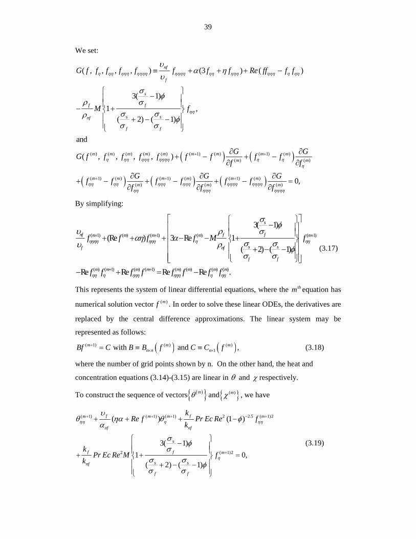
We set:
( ) ( )( ) ( ) ( ) ( ) ( ) ( 1) ( ) ( 1) ( )( ) ( )
( , , , , ) (3 ) ( )
3( 1)
1 ,( 2) ( 1)
and
( , , , , )
nf
f
s
f f
s snf
f f
m m m m m m m m m
m m
G f f f f f f f f Re ff f f
M f
G GG f f f f f f f f f
f f
η ηη ηηη ηηηη ηηηη ηη ηηη ηηη η ηη
ηη
η ηη ηηη ηηηη η ηη
υα η
υ
σφ
ρ σσ σρ φσ σ
+ +
≡ + + + −
−
− +
+ − −
∂ ∂+ − + −
∂ ∂
( ) ( ) ( )( 1) ( ) ( 1) ( ) ( 1) ( )( ) ( ) ( )
0,m m m m m m
m m m
G G Gf f f f f f
f f fηη ηη ηηη ηηη ηηηη ηηηηηη ηηη ηηηη
+ + +∂ ∂ ∂+ − + − + − =
∂ ∂ ∂
By simplifying:
( 1) ( ) ( 1) ( ) ( 1)
( ) ( 1) ( ) ( 1) ( ) ( ) ( ) ( )
3( 1)
(Re ) 3 Re 1( 2) ( 1)
Re Re Re Re .
s
nf f fm m m m m
s sf nf
f f
m m m m m m m m
f f f f M f
f f f f f f f f
ηηηη ηηη η ηη
ηη η ηηη ηηη η ηη
σφ
υ ρ σαη α
σ συ ρ φσ σ
+ + +
+ +
−
+ + + − − + + − −
− + = −
(3.17)
This represents the system of linear differential equations, where the thm equation has
numerical solution vector( )mf . In order to solve these linear ODEs, the derivatives are
replaced by the central difference approximations. The linear system may be
represented as follows:
( ) ( )( 1) ( ) ( )1 with and ,m m m
n n nBf C B B f C C f+× ×= ≡ ≡ (3.18)
where the number of grid points shown by n. On the other hand, the heat and
concentration equations (3.14)-(3.15) are linear in θ and χ respectively.
To construct the sequence of vectors( ) mθ and ( )mχ , we have
( 1) ( 1) ( 1) 2 2.5 ( 1)2
2 ( 1)2
( ) (1 )
3( 1)
1 0,( 2) ( 1)
f fm m m m
nf nf
s
f f m
s snf
f f
kRe f Pr Ec Re f
k
kPr Ec Re M f
k
ηη η ηη
η
υθ ηα θ φ
α
σφ
σσ σ
φσ σ
+ + + − +
+
+ + + −
− + + =
+ − −
(3.19)

40
( 1) ( 1) ( 1)( ) 0,m m mRe f Scηη ηχ χ ηα+ + ++ + = (3.20)
It is worth mentioning that ( 1)mf + is observed to be known and its derivatives are
replaced by approximations.
We list out the computational procedure as under:
o Provide the values of ( ) ( ) ( )0 0 0, &f θ χ as initial guess satisfying the boundary
conditions given in Eq. (3.16) ,
o The linear system (Eq. (3.18)) is solved to calculate ( )1f
o Using the value of ( )1f in Eqs. (3.19) - (3.20). After solving these equations,
we obtain ( ) ( )1 1&θ χ .
o The procedure is repeated by taking initial guess to generate the sequences
( ) ( ) ( )1 1 1, &f θ χ that respectively converge to , &f g θ which represent the
solution of Eqs. (3.13)-(3.15).
o The sequences of vectors are generated until
( ) ( ) ( ) ( ) ( ) ( ) 1 1 1 6max , , 10 .m m m m m m
L L Lf f θ θ χ χ
∞ ∞ ∞
+ + + −− − − <
Further details about the computational procedure may be reviewed from Ali et al.
[104-106].
3.4. RESULTS AND DISCUSSION
The Reynolds numbers Re, the Schmidt number Sc , the.magnetic.parameterM ,
nano-particle. volume fraction. parameterφ , the Eckert numberEc and the wall
expansion ratioα are parameters for the problem under investigation. The upper and
lower walls are expanding or contracting with time-dependent rate )(ta′ and having
same permeability. We suggest the nano-fluid based on water which contains 2 3Al O
nano-particle. For the flow, heat and concentration problem under consideration, the
following set of values are taken
( )12997.1, 10 , 3970, 25, 0.613, 0.05, 765,f s s s f f p sk k c andρ σ ρ σ−= = = = = = =
Pr 6.2.= The case 0=φ stands for pure water.
In case of both moving away or approaching walls 0>α or 0<α respectively. The
parameter 0R e > for injection. We are going to study the velocities ( )ηf & ( )ηf ′ ,

41
temperature field ( )ηθ and the concentration filed ( )χ η against set of values of some
parameters of physical nature. The flow stream lines are shown in Fig. 3.2.
In Figs. 3.3-3.6, influence of the applied magnetic field upon velocity and temperature
profiles is shown. The streamwise velocity is an increasing function whereas the
temperature is a decreasing function of applied magnetic field, irrespective of the
walls motion. The nano-particles volume fraction has negligible effect on the velocity
field. The temperature of the fluid is increasing for receding walls whereas an
opposite trend is observed for approaching walls. However, the change in the
temperature for approaching walls is significant as compare to that of receding walls.
These trends may be noted in Figs. (3.7-3.10).
The influence of the permeability Reynolds number on the flow velocity,
concentration and temperature distribution can be observed graphically from Figs.
3.11-3.16. Maximum velocity is obtained when both the walls are contracting in the
central region between the channel walls. However, this trend is reversed in case of
the expanding the walls. The increase in Re has the influence of rising temperature in
the whole domain for 0α > , whereas in case of the approaching walls, Re has non
uniform effect on the temperature. In both the cases whetherα is positive or negative,
the behaviour of Re on ( )χ η′ remains the same.
As α changes from positive to negative, there is a significant rise in highest value of
velocity while, on the other hand, temperature profiles are remarkably lowered.
Moreover, concentration profile is increasing in the lower half whereas it is
decreasing in the upper half of the channel. These may be observed in Figs. 3.17-3.19.
The Eckert number characterizes the viscous dissipation as shown in Figs. 3.20-3.21.
It has significant rise in the temperature profiles during the contraction or expansion
of the walls. Further, in approaching walls, the Eckert number has more remarkable
effect. Figures 3.22-3.23 clearly show that the concentration profiles have linear
variation against the Schmidt number.
Numerical results are well arranged as the step-size decreases. The convergence of the
results for the flow velocity is shown in Table 3.1. This convergence has significant
role in processing of our computational procedure. Shear stress along with heat and
mass transfer rates at the walls of the channel are increased as the external magnetic
field increases. This may be observed in Table 3.2. When we consider the problem of
approaching walls, it is noted that( 1)θ ′ − is more affected by magnetic field. This is
42
due to the Lorentz force which tends to drag fluid towards disk. The magnetic field
exerts a retarding force named as friction. This increases the shear stress at the walls
of the channel. Moreover, the fluid temperature and the temperature difference
increase due to the frictional force, between the walls and the .fluid. The heat transfer
rate, being directly .proportional to the. temperature difference, also increases.
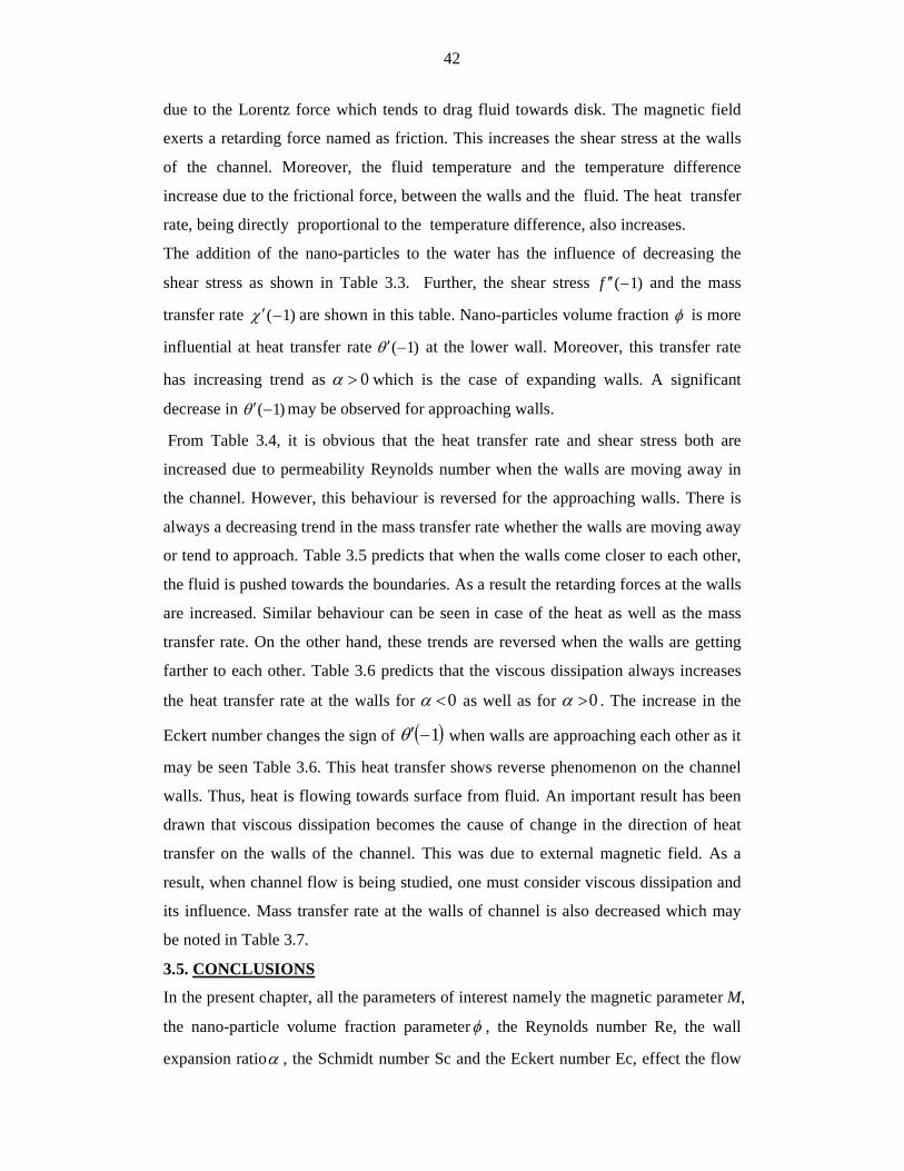
The addition of the nano-particles to the water has the influence of decreasing the
shear stress as shown in Table 3.3. Further, the shear stress ( 1)f ′′ − and the mass
transfer rate ( 1)χ ′ − are shown in this table. Nano-particles volume fraction φ is more
influential at heat transfer rate ( 1)θ ′ − at the lower wall. Moreover, this transfer rate
has increasing trend as 0α > which is the case of expanding walls. A significant
decrease in ( 1)θ ′ − may be observed for approaching walls.
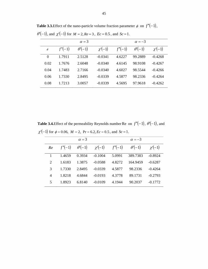
From Table 3.4, it is obvious that the heat transfer rate and shear stress both are
increased due to permeability Reynolds number when the walls are moving away in
the channel. However, this behaviour is reversed for the approaching walls. There is
always a decreasing trend in the mass transfer rate whether the walls are moving away
or tend to approach. Table 3.5 predicts that when the walls come closer to each other,
the fluid is pushed towards the boundaries. As a result the retarding forces at the walls
are increased. Similar behaviour can be seen in case of the heat as well as the mass
transfer rate. On the other hand, these trends are reversed when the walls are getting
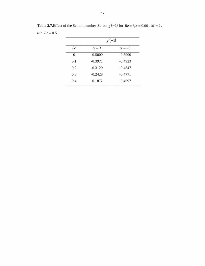
farther to each other. Table 3.6 predicts that the viscous dissipation always increases
the heat transfer rate at the walls for 0<α as well as for 0>α . The increase in the
Eckert number changes the sign of ( )1−′θ when walls are approaching each other as it
may be seen Table 3.6. This heat transfer shows reverse phenomenon on the channel
walls. Thus, heat is flowing towards surface from fluid. An important result has been
drawn that viscous dissipation becomes the cause of change in the direction of heat
transfer on the walls of the channel. This was due to external magnetic field. As a
result, when channel flow is being studied, one must consider viscous dissipation and
its influence. Mass transfer rate at the walls of channel is also decreased which may
be noted in Table 3.7.
3.5. CONCLUSIONS
In the present chapter, all the parameters of interest namely the magnetic parameter M,
the nano-particle volume fraction parameter , the Reynolds number Re, the wall
expansion ratio , the Schmidt number Sc and the Eckert number Ec, effect the flow
φ
α

43
as well as the heat and mass transfer characteristics of the laminar incompressible
nano-fluid (based on water (containing 2 3Al O nano-particles)) through a channel. The
following conclusions may be drawn:
Forα > 0:
1) The shear stress is enhanced by M and Re while an opposite trend is observed
for and α .
2) The parameters M, Re and φ increase the heat transfer rate but this trend is
reversed in case of .
3) Re and Sc have the effect of decreasing the mass transfer rate while it is
increased by the applied magnetic field.
Forα < 0:
4) The magnetic field increases the heat transfer rate as well as the shear stress
whereas both the volume fraction and the permeability have opposite trend as
that of the external magnetic field.
5) Mass transfer is reduced by the Schmidt number, permeability Reynolds
number and volume fraction. On the other hand, both α and M make the shear
stress larger at the walls .
φ
α

44
Table 3.1. Dimensionless velocity ( )ηf on three grid sizes and extrapolated values
for 3, 0.06, 3Re φ α= = = − , 2M = , 0.5Ec = , and 1Sc = .
( )ηf
η 1st grid
( 0.02)h =
2nd grid
( 0.01)h =
3rd grid
( 0.005)h =
Extrapolated
values
0
0.2
0.4
0.6
0.8
0
0.2613
0.5135
0.7425
0.9218
0
0.2613
0.5136
0.7426
0.9219
0
0.2614
0.5136
0.7426
0.9219
0
0.2614
0.5136
0.7427
0.9219
Table 3.2. Effect of the magnetic parameter M on ( )1−′′f , ( )1−′θ , and ( )1' −χ for
0.06, 3Reφ = = , 2.0=Ec , and 1Sc = .
3α = 3α = −
M ( )1−′θ ( )1' −χ ( )1−′′f ( )1−′θ ( )1' −χ
0.5
1
1.5
2
2.5
1.5940
1.6408
1.6871
1.7330
1.7784
2.4363
2.5719
2.7097
2.8495
2.9914
-0.0335
-0.0337
-0.0338
-0.0339
-0.0340
4.4625
4.5047
4.5464
4.5877
4.6285
82.5751
87.7415
92.9614
98.2336
103.5568
-0.4251
-0.4255
-0.4260
-0.4264
-0.4269
( )1−′′f
45
Table 3.3.Effect of the nano-particle volume fraction parameter φ on ( )1−′′f ,
( )1−′θ , and ( )1' −χ for 2, 3M Re= = , 0.5Ec = , and 1Sc = .
3α = 3α = −
( )1−′θ ( )1' −χ ( )1−′′f ( )1−′θ ( )1' −χ
0
0.02
0.04
0.06
0.08
1.7911
1.7676
1.7483
1.7330
1.7213
2.5128
2.6048
2.7166
2.8495
3.0057
-0.0341
-0.0340
-0.0340
-0.0339
-0.0339
4.6227
4.6145
4.6027
4.5877
4.5695
99.2889
98.9108
98.5544
98.2336
97.9618
-0.4268
-0.4267
-0.4266
-0.4264
-0.4262
Table 3.4.Effect of the permeability Reynolds numberRe on ( )1−′′f , ( )1−′θ , and
( )1' −χ for 0.06,φ = 2,M = Pr 6.2, 0.5Ec= = , and 1Sc = .
3α = 3α = −
Re ( )1−′θ ( )1' −χ ( )1−′′f ( )1−′θ ( )1' −χ
1
2
3
4
5
1.4659
1.6183
1.7330
1.8218
1.8923
0.3934
1.3875
2.8495
4.6844
6.8140
-0.1004
-0.0588
-0.0339
-0.0193
-0.0109
5.0991
4.8272
4.5877
4.3778
4.1944
389.7383
164.9459
98.2336
89.1731
90.2037
-0.8924
-0.6287
-0.4264
-0.2793
-0.1772
φ ( )1−′′f
( )1−′′f

46
Table 3.5. Effect of the wall expansion ratioα on ( )1−′′f , ( )1−′θ , and ( )1' −χ for
0.06, 3, 2Re Mφ = = = , 0.5Ec = , and 1Sc = .
α ( )1−′θ ( )1' −χ
-4
-2
0
2
4
5.1827
4.0173
2.9751
2.0998
1.4145
307.2624
46.7843
14.6338
4.9287
1.6353
-0.6039
-0.2936
-0.1302
-0.0538
-0.0211
Table 3.6. Effect of the Eckert numberEc on ( )1−′θ for 3, 0.06Re φ= = , 2M = , and
1Sc = .
( )1−′θ
Ec 3α = 3α = −
0
0.1
0.2
0.3
0.4
0
0.5699
1.1398
1.7097
2.2796
-0.2001
19.4867
39.1734
58.8601
78.5468
( )1−′′f
47
Table 3.7.Effect of the Schmit number Sc on ( )1' −χ for 3, 0.06Re φ= = , 2M = ,
and 0.5Ec = .
( )1' −χ
Sc 3α = 3α = −
0
0.1
0.2
0.3
0.4
-0.5000
-0.3971
-0.3120
-0.2428
-0.1872
-0.5000
-0.4923
-0.4847
-0.4771
-0.4697

48
Figure 3.1 Physical model of the problem.
Figure 3.2 Streamlines for the problem forRe 6= , 0.06φ = , 3α =− and 2M = .

49
Figure 3.3 Streamwise velocity profiles forRe 3= , 0.06φ = , 3α = , 0.5Ec = and
1=Sc .
Figure 3.4 Temperature profiles forRe 3= , 0.06φ = , 3α = , 0.5Ec = and 1=Sc .

50
Figure 3.5 Streamwise velocity profiles forRe 3= , 0.06φ = , 3α = − , 0.5Ec = and
1=Sc .
Figure 3.6 Temperature profiles for Re 3= , 0.06φ = , 3α = − , 0.5Ec = and 1=Sc .

51
Figure 3.7 Streamwise velocity profiles for Re 3= , 3α = , 0.5Ec = , 1=Sc
and 2M = .
Figure 3.8 Temperature profiles for Re 3= , 3α = , 0.5Ec = , 1=Sc and 2M = .

52
Figure 3.9 Streamwise velocity profiles forRe 3= , 3α = − , 0.5Ec = , 1=Sc
and 2M = .
Figure 3.10 Temperature profiles forRe 3= , 3α = − , 0.5Ec = , 1=Sc and
2M = .

53
Figure 3.11 Streamwise velocity profiles for 3α = , 0.06φ = , 0.5Ec = , 1=Sc
and 2M = .
Figure 3.12 Temperature profiles for 3α = , 0.06φ = , 0.5Ec = , 1=Sc and
2M = .
54
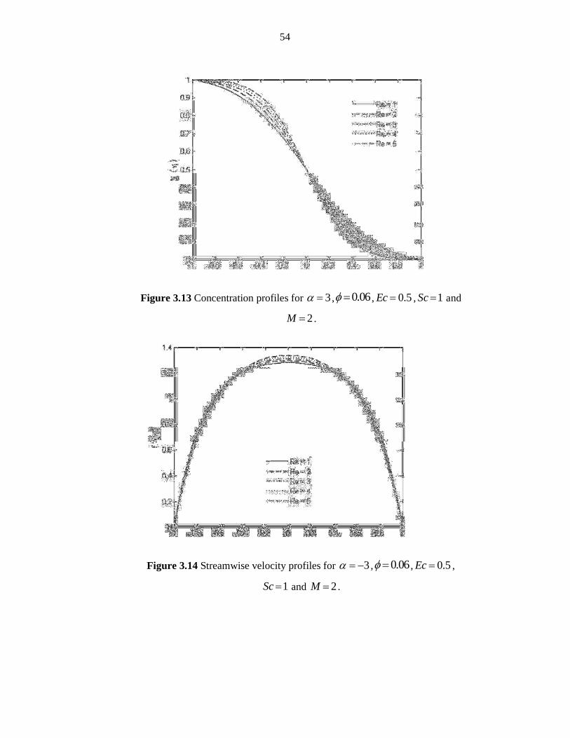
Figure 3.13 Concentration profiles for 3α = , 0.06φ = , 0.5Ec = , 1=Sc and
2M = .
Figure 3.14 Streamwise velocity profiles for 3α = − , 0.06φ = , 0.5Ec = ,
1=Sc and 2M = .

55
Figure 3.15 Temperature profiles for 3α = − , 0.06φ = , 0.5Ec = , 1=Sc and
2M = .
Figure 3.16 Concetration profiles for 3α = − , 0.06φ = , 0.5Ec = , 1=Sc and
2M = .

56
Figure 3.17 Streamwise velocity profiles for 0.06φ = ,Re 3= , 0.5Ec = , 1=Sc
and 2M = .
Figure 3.18 Temperature profiles for 0.06φ = ,Re 3= , 0.5Ec = , 1=Sc and
2M = .

57
Figure 3.19 Concentration profiles for 0.06φ = ,Re 3= , 0.5Ec = , 1=Sc and
2M = .
Figure 3.20 Temperature profiles for 0.06φ = ,Re 3= , 3α = , 1=Sc and
2M = .
58
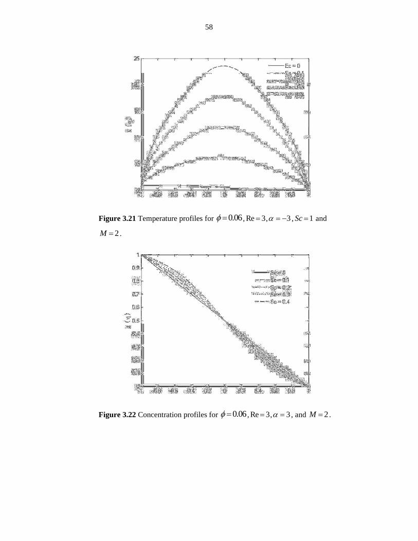
Figure 3.21 Temperature profiles for 0.06φ = ,Re 3= , 3α = − , 1=Sc and
2M = .
Figure 3.22 Concentration profiles for 0.06φ = ,Re 3= , 3α = , and 2M = .

59
Figure 3.23 Concentration profiles for 0.06φ = ,Re 3= , 3α = − , and 2M = .

60
CHAPTER NO 4
ON THE NON–NEWTONIAN FLUID FLOW DRIVEN BY
A CURVED STRETCHING SHEET

61
4.1. INTRODUCTION
MHD, Non-Newtonian and electrically conducting fluid flow subject to a magnetic
field applied transversely over a circular coiled curved stretching sheet is addressed in
the present chapter. For mathematical modelling, the well-known Casson fluid model
has been employed. The governing nonlinear differential equations are solved
numerically by employing an algorithm based on the Quasi-linearization method.
Physical parameters of the problem in terms of skin-friction coefficient, local Nusselt
number, flow velocity and thermal profiles are discussed through tables and graphs.
4.2. MATHEMATICAL FORMULATION
Let us consider the flow and heat transfer in 2-dimensional steady &
incompressible Casson fluid flow over a circular coiled curved stretching sheet of
radius R . The curved sheet is stretched with the fixed origin, due to the action of two
forces (equal in the magnitude but opposite in the direction) acting along the s -
direction. Further, the s andr -directions are perpendicular to each other. Where
u as= is velocity of the stretching surface & the strength of the stretching is 0a > .
The fluid has the property of electrical conduction & magnetic field applied in “r ”
direction having constant intensity 0B . The magnetic Reynolds number is assumed
really small with the intention that the induced magnetic field can be ignored. The
surface temperature is kept carefully atwT , keeping wT T∞> and T∞ is the uniform
temperature of the fluid far away. With these assumptions in addition to the
approximations of boundary layer, the governing equations of the Casson fluid flow
(taking into account the influence of the resistive Lorentz force) are given below:
The Continuity Equation
( ) 0u
r R v Rr s
∂ ∂+ + =
∂ ∂ (4.1)
s- Component of the Momentum Equation
2
.1u p
r R rρ∂
=+ ∂
(4.2)
r- Components of the Momentum Equation
2
2
20
2
1 1(1 )(
1) ,
( )
u Ru u uv uv
r r R s r R r r R
Bu u R pu
r r R r R s
υβ
σρ ρ
∂ ∂ ∂+ + = + +
∂ + ∂ + ∂ +
∂ ∂− − −
∂ + + ∂
(4.3)

62
The Heat Equation
2
0 2
22 20
1
1(1 )( ) ,
p
T uR T T Tc v K
r r R s r r R r
Buu
r
ρ
σµ
β ρ
∂ ∂ ∂ ∂ + = + ∂ + ∂ ∂ + ∂
∂− + +
∂
(4.4)
where the symbols u and v are the components of the velocity in s and r -directions,
correspondingly, ρ is the fluid density, µ is the fluid viscosity, p is the pressure, υ
is the kinematics viscosity of fluid, σ is the electrical conductivity, pc is the heat
(specific) keeping the pressure constant, thermal conductivity is 0k & T is the
temperature. It is noted that, for a stretching curved surface, inside the boundary layer
the pressure is no more constant (Sajid et al. [107]).
The suitable boundary conditions under are
0 , 0, ,
0, 0, .
wat r u as v T T
uas r u T T
r ∞
= = = =
∂→∞ → → →
∂
(4.5)
For simplifying and converting the flow and heat equations into ordinary ones, the
following dimensionless variables may be introduced
2 2
( ), ( ), ,
( ), ( ) .w
R au asf v a f r
r RT T
p a s PT T
η υ η ηυ
ρ η θ η ∞
∞
−′= = =
+−
= =−
(4.6)
Equation (4.1) is satisfied automatically whereas the equations (4.2) - (4.4) yield to
2p f
kη η′∂
=∂ +
, (4.7)
( )
( )
22
22
2 1(1 )
k k f fP f f
k k k k
k kff M f ff
k k
η η β η η
η η
′′ ′′ ′′′= − + + + −
+ + + +
′′ ′ ′+ − ++ +
, (4.8)
221 1
Pr 1 (1 ) Pr1
(1 )
k Mf Ec f
k kθ θ
η η ββ
′′ ′ ′= − − + − + + + +
, (4.9)

63
These equations include ak R υ= as radius of curvature and 2 20 /M B aσ ρ= is the
Hartmann number, 0
Pr pck
µ= is the Prandtl number,
2( )c
p
asE c T=
is the Eckert
number.
On exclusion of pressure term from equations (4.7) and (4.8), one can obtain
( ) ( ) ( )
( )( )
( )( )
( )
3 2
2
22 3
1 2(1 )
0
iv f f ff
k k k
f kM f f f f f
k k
k kf f f ff
k k
β η η η
η η
η η
′′′ ′ ′′+ + + −
+ + +
′′′ ′ ′′ ′′′− + − −
+ +
′′ ′ ′− − + − =+ +
, (4.10)
As the velocity ( )f η of the fluid is obtained, the pressure term can be determined
from equation (4.8) as given below:
( ) ( )
( )
2
2 2 22
1(1 )
2
k f fP f
k k k
k k kf M f f f f f
k k k
ηβ η η
η η η
′′ ′+ ′′′= + + − + +
′ ′ ′′ ′− − + ++ + +
, (4.11)
On the other hand, the corresponding boundary conditions at the surface and far from
the sheet become:
(0) 0, (0) 1, (0) 1,
( ) 0, ( ) 0, ( ) 0.
f f
f f
θθ
′= = =
′ ′′∞ = ∞ = ∞ = (4.12)
From engineering point of view, the physical quantities here are the local Nusselt
number in the s -direction and the skin friction coefficient which may be respectively
described, mathematically, as
2rs
fw
Cu
τρ
= , 1( )
ws
w
sqNu
k T T∞
=−
, (4.13)
These expressions have the shear stress at the wall as rsτ , and the thermal flux at. the
wall as wq which are specified as
1(1 )( )rs
u u
r r Rτ µ
β∂
= + −∂ +
at 0r =
1w
Tq k
r
∂=−
∂at 0r = (4.14)

64
Equation (4.13), after using equations (4.6) and (4.14), may be written as
12 1 (0)
Re (1 ) (0)f s
fC f
kβ′ ′′= + − +
,
1
2Re (0)s sNu θ−
′= − .
The local Reynolds number is 2
.es
asR
υ= .
4.3. NUMERICAL SOLUTION
The governing equations (4.9) and (4.10), on applying Quasi-linearization
(please see chapter 2), take the form:
21 1 12
1 1 1Pr 1 (1 ) Pr
1(1 )
j j jjk Mf Ec f
k kθ θ
η η ββ
+ + ++
′′ ′ ′= − − + − + + + +
(4.15)
( )
( )
( ) ( )
( ) ( ) ( ) ( ) ( )
( ) ( ) ( )
1 1
1
1
22 2
23 2 3
2 3
1 1 11 2 1
1 11
1 1 1 21
j j
j
j
j j
iv j
j j
j j j
j
kf f f
k k
k kM f f f
kk k
k k kM f f f f
k kk k k
k k kf f f
k k k
β β η η
β ηη η
β η ηη η η
η η η
+ +
+
+
′′′+ + + + + +
′ ′′+ − + − − + ++ +
′ ′′ ′+ + − − − − + ++ + +
′′′ ′′ ′+ + −
+ + + ( )
( )( )
( )
1
2 3 0
j j j
j j j
j j
j j
kf f f f f
k
k kf f f f f
k k
η
η η
+ ′′′ ′ ′′= −+
′′ ′ ′+ − − =+ +
(4.16)
The approximations of central difference, when utilized for the derivatives in the
equations given above, yield the following systems of algebraic equations which may
then be solved by using some standard method for matrix inversion.
( ) ( ) ( )1 1
2
2 21 1
1 12 4 2
1Pr 1 2
2
j j ji i i
k ki i
k kh h
k k k k
f fh M Ec
θ θ θη η η η
β
− +
+ −
− − − + + − + + + +
− = + −
(4.17)

65
( ) ( 1) ( 1)2 1
( ) ( 1) 21
( ) ( )2 1 1
2 2
1 1 1 12 1 2 1 8 1
1 12 2 1 2
1 1 11 1
( ) ( ) 2 ( )
j j ji i i
j ji i
j ji i
i
kh f f f
k k
kh f f h
k k
f fk kM f
k k h k
β β η η β
β η η
β η β η η
+ +− −
+−
+ −
+ − + + − + + +
+ + + + + +
−− + − + − + + + +
( ) ( 1) 31
( ) ( ) ( ) ( ) ( )1 1 1 1
3 2 2
( 1)1( ) ( )
21 13
( 1) 2
21 21
( ) ( ) ( ) 2
1
( ) 2
112 1 4
11
j ji
j j j j ji i i i i
jij j
i i
ji
f h
f f f f fk k k
k k h k hf
f fkM
k h k
f h
β η η η
η η
β
+−
+ − + −
+−
+ −
+
−
− + −+ − − + + +
− − − + +
+ + −
− +( ) ( )
2 ( ) ( 1)1 12 2
( ) ( ) ( ) ( ) ( ) ( ) ( )2 1 1 2 1 1
3 2 2
4
( ) ( )1 1
3
1 11
( ) ( ) 2 ( )
2 2 2
( ) 2 ( )2
( )
j jj ji i
i i
j j j j j j ji i i i i i i
j ji i
f fk kM f f
k k h k
f f f f f f fk k
k h k hh
f fk
k
β η β η η
η η
η
++ −
+ + − − + −
+ −
− − + − + + + +
− + − − ++ + +
+−
−+
( 1)
( )
( 1) ( ) ( 1) 21 1
( ) ( )2 ( ) ( 1) 31 1
12 2
2
1 1 18 1 2 2 1 2
( ) ( )
1 11
( ) ( ) 2 ( )
11
ji
ji
j j ji i i
j jj ji i
i i
f
fh
kf h f f h
k k
f fk kM f f h
k k h k
β β η η
β η η η
β
+
+ ++ +
++ −+
− + − + + − + +
− − + − − + + + + +
+
( ) ( ) ( ) ( ) ( )1 1 1 1
3 2 2
( 1)1( ) ( )
21 13
( )
2 2
( ) ( ) ( ) 2
1
( ) 2 ( )
1 1 12 1 2 1
( ) ( )
j j j j ji i i i i
jij j
i i
ji i
f f f f fk k k
k k h k hf
f fkM
k h k
kh f f
k k
η η η
η η
β β η η
+ − + −
++
+ −
− + −− − + + +
− − − + +
+ + + + + + +
( 1)2 ( )j k
hkη
++ =
+
(4.18)
( ) ( )( )
( ) ( )
( )
( ) ( ) ( ) ( ) ( ) ( ) ( ) ( ) ( ) ( )2 1 1 2 1 1 1 1 2
22( ) ( ) ( ) ( ) ( ) ( ) ( )
2 1 1 2 1 1
3 ( ) ( ) ( )1 13
2 2 2( )
2 22
( )
j j j j j j j j j ji i i i i i i i i i
j j j j j j ji i i i i i i
j j ji i i
kf f f f f f f f f f
k
hh f f f f f f f
kh f f f
k
η
η
+ + − − + − + −
+ + − − + −
+ −
− + − − − − + + +
− + − − − −
− +

66
4.4. RESULTS AND DISCUSSION
For understanding impact of various parameters to govern the coefficient of
skin-friction & heat transfer, numerical solution of the system of ODE’s (4.9) & (4.10)
along with the boundary conditions (4.12) has been obtained by employing the
numerical procedure mentioned above, for the various values of the governing
parameters (M, β , k , Pr, and Ec).
Table 4.1 shows the 1
2Res fC for the various values of the β . It is easy to see that, by
increasing the values of β , the magnitude of 1
2Res fC may decrease while increasing
the heat transfer at the curved sheet. It may be noted from the Table 4.2 that the
external magnetic field raises the skin-friction coefficient while lowering the heat
transfer at the sheet. Dependence of the heat transfer over the Prandtl number and the
Eckert number may be observed from the Tables 4.3 and 4.4. Obviously, both the
numbers tend to raise the heat transfer rate at the curved sheet. Table 4.5 shows how
the dimensionless curvature κ affects the skin-friction and the heat transfer. Clearly,
the parameter remarkably decreases both the physical quantities. However, the
dependence of the quantities on κ is much stronger when κ is nearer to unity.
We observe from the Figures 4.2 and 4.3 that, by raising values of the β , the fluid
velocity distribution decreases. With an increase in the β , the fluid yields stress
causing a resistance force which slows down the fluid motion. The temperature
profiles for different increasing values of the β for the curved sheet are shown in Fig
4.4. This figure shows that the Casson nature of the fluid lowers the fluid temperature
to such an extent that it goes beyond the temperature of the ambient fluid. Figures 4.5
and 4.6 show that M has the decreasing effect on both the velocity components while
raising its temperature as shown in Fig 4.7. It is because of the fact that the imposed
magnetic field acts normal to the direction of the flow, and thus induces the drag in
terms of the Lorentz force which retards the flow while increasing its temperature.
Hence, the external magnetic field bears the potential to enhance the temperature of
the fluid as it may be compared with literature work of Misra & Sinha [108]. Figure
4.8 reflects the influence of Pr on dimensionless temperature. As expected, the
increasing Pr leads to the reduction in the dimensionless temperature. As Pr raises, the
heat diffusivity reduces which leads to the decrease of energy ability that decreases
the thermal boundary layer (Ali et al. [109]). The effect of the Eckert number Ec on

67
the (0)θ ′− is shown in Fig. 4.9. It is clear that the thermal profiles decrease with an
increase in the viscous dissipation (quantified by the Eckert number).
Figures 4.10 and 4.11 depict the distribution of the velocity for different
values of the curvature parameter K. Here the fluid velocity is enhanced as K is
increased. In fact for higher values of curvature parameter, the stretching strength of
the sheet increases (for the fixed radius of the sheet), which enhances the fluid flow.
Fig. 4.12 shows that the dimensionless curvature parameter K has the ability to
balance the tremendous lowering of the thermal distribution due to the Casson nature
of the fluid with larger Pr.
4.5. CONCLUSIONS
The MHD flow and the (0)θ ′− of a Casson fluid passes through the curved sheet
coiled in a circle, subject to the governing parameters (namely M, β , k , Pr, and Ec)
is analysed here. Main findings of the present study can be summarized as:
1) The Casson parameter reduces the velocity as well as the temperature
distribution.
2) The magnetic parameter decreases both the velocity components while raising
the fluid temperature.
3) Effect of both the Prandtl number and the Eckert number is to raise the
temperature profile.
4) The curvature parameter may act as a neutralising agent to balance the
remarkable lowering of the temperature profile, due to the Casson nature of
the fluid at larger Prandtl number.

68
Table 4.1. Variation of 1
2Res fC and (0)θ ′− for 0.5M = , 7κ = , Pr 21= , and 1Ec =
against β .
Sr. No. β 1
2Res fC (0)θ ′−
1 0.2 -3.8400 3.4658
2 0.6 -2.3165 5.2456
3 0.9 -2.0183 5.9439
4 1.2 -1.8594 6.4161
5 1.4 -1.7888 6.6554
Table 4.2. Variation of1
2Res fC and (0)θ ′− for 2β = , 7κ = , Pr 21= and 1Ec =
against M .
Sr. No. M 1
2Res fC (0)θ ′−
1 0 -1.4748 8.2657
2 0.6 -1.7231 7.4712
3 1.2 -2.2397 5.5307
4 1.8 -2.8496 3.1137
5 2.4 -3.4949 0.4836
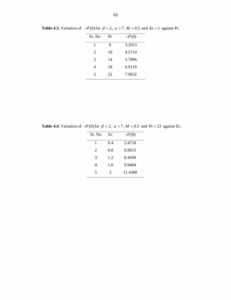
69
Table 4.3. Variation of (0)θ ′− for 2β = , 7κ = , 0.5M = and 1Ec = against Pr.
Sr. No Pr (0)θ ′−
1 6 3.2013
2 10 4.5714
3 14 5.7896
4 18 6.9118
5 22 7.9632
Table 4.4. Variation of (0)θ ′− for 2β = , 7κ = , 0.5M = and Pr 21= against Ec.
Sr. No Ec (0)θ ′−
1 0.4 5.4718
2 0.8 6.9613
3 1.2 8.4509
4 1.6 9.9404
5 2 11.4300
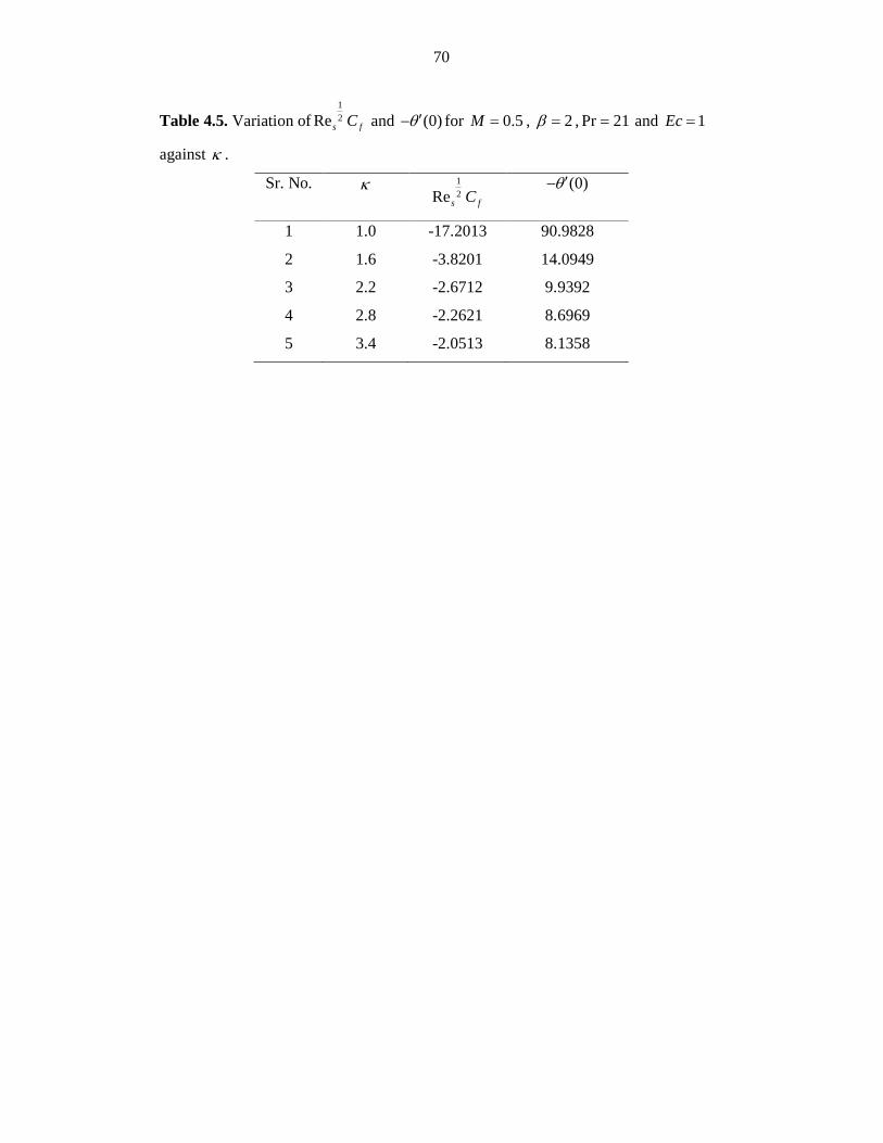
70
Table 4.5. Variation of1
2Res fC and (0)θ ′− for 0.5M = , 2β = ,Pr 21= and 1Ec =
against κ .
Sr. No. κ 1
2Res fC (0)θ ′−
1 1.0 -17.2013 90.9828
2 1.6 -3.8201 14.0949
3 2.2 -2.6712 9.9392
4 2.8 -2.2621 8.6969
5 3.4 -2.0513 8.1358
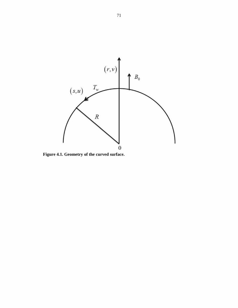
71
Figure 4.1. Geometry of the curved surface.

72
0 2 4 6 8 10 12 14 16 18 200
0.5
1
1.5
2
2.5
η
f
( η )
β = 0.2
β = 0.6
β = 0.9
β = 1.2
β = 1.4
Figure 4.2. Axial velocity profiles for 7κ = , 0.5M = ,Pr 21= , 1Ec = .
0 2 4 6 8 10 120
0.1
0.2
0.3
0.4
0.5
0.6
0.7
0.8
0.9
1
η
f '
( η )
β = 0.2
β = 0.6
β = 0.9
β = 1.2
β = 1.4
Figure 4.3. Radial velocity profiles for 7κ = , 0.5M = ,Pr 21= , 1Ec = .

73
0 0.5 1 1.5 2 2.5 3 3.5 4-0.4
-0.2
0
0.2
0.4
0.6
0.8
1
η
θ (
η )
β = 0.2
β = 0.6
β = 0.9
β = 1.2
β = 1.4
Figure 4.4. Temperature profiles for 7κ = , 0.5M = ,Pr 21= , 1Ec = .
0 2 4 6 8 10 12 14 16 18 200
0.2
0.4
0.6
0.8
1
1.2
1.4
η
f
( η )
M = 0
M = 0.6
M = 1.2M = 1.8
M = 2.4
Figure 4.5. Axial velocity profiles for 7κ = , 2β = ,Pr 21= , 1Ec = .

74
0 1 2 3 4 5 6 7 8 9 10-0.1
0
0.1
0.2
0.3
0.4
0.5
0.6
0.7
0.8
0.9
η
f '
( η )
M = 0
M = 0.6
M = 1.2M = 1.8
M = 2.4
Figure 4.6. Radial velocity profiles for 7κ = , 2β = ,Pr 21= , 1Ec = .
0 0.5 1 1.5 2 2.5 3 3.5 4-0.4
-0.2
0
0.2
0.4
0.6
0.8
1
η
θ (
η )
M = 0
M = 0.6
M = 1.2M = 1.8
M = 2.4
Figure 4.7. Temperature profiles for 7κ = , 2β = ,Pr 21= , 1Ec = .

75
0 0.2 0.4 0.6 0.8 1 1.2 1.4 1.6 1.8 2-0.4
-0.2
0
0.2
0.4
0.6
0.8
1
η
θ (
η )
Pr = 6
Pr = 10
Pr = 14Pr = 18
Pr = 22
Figure 4.8. Temperature profiles for 7κ = , 2β = , 0.5M = , 1Ec = .
0 0.2 0.4 0.6 0.8 1 1.2 1.4 1.6 1.8 2-0.8
-0.6
-0.4
-0.2
0
0.2
0.4
0.6
0.8
1
η
θ (
η )
Ec = 0.4
Ec = 0.8
Ec = 1.2Ec = 1.6
Ec = 2
Figure 4.9. Temperature profiles for 7κ = , 2β = , 0.5M = ,Pr 21= .

76
0 2 4 6 8 10 12 14 16 18 200
0.2
0.4
0.6
0.8
1
1.2
1.4
η
f
( η )
κ = 1.0
κ = 1.6
κ = 2.2
κ = 2.8
κ = 3.4
Figure 4.10. Axial velocity profiles for 0.5M = , 2β = ,Pr 21= , 1Ec = .
0 1 2 3 4 5 6 7 80
0.1
0.2
0.3
0.4
0.5
0.6
0.7
0.8
0.9
1
η
f '
( η )
κ = 1.0
κ = 1.6
κ = 2.2
κ = 2.8
κ = 3.4
Figure 4.11. Radial velocity profiles for 0.5M = , 2β = ,Pr 21= , 1Ec = .

77
0 0.2 0.4 0.6 0.8 1 1.2 1.4 1.6 1.8 2-4
-3.5
-3
-2.5
-2
-1.5
-1
-0.5
0
0.5
1
η
θ (
η )
κ = 1.0
κ = 1.6
κ = 2.2
κ = 2.8
κ = 3.4
Figure 4.12. Temperature profiles for 0.5M = , 2β = ,Pr 21= , 1Ec = .
78
CHAPTER 5
ON THE SUITABILITY OF ROSSELAND
APPROXIMATION FOR THERMAL RADIATION IN
FLOW OVER A ROTATING CONE EMBEDDED IN
POROUS MEDIUM

79
5.1. INTRODUCTION
Flow, heat and mass transfer of MHD Casson fluid over a vertical rotating cone
through porous medium containing gyrotactic microorganisms in the presence of
Soret and Dufour effects are investigated numerically. A comparative study has been
taken into account between linear and nonlinear approaches of the Rosseland
approximation for the thermal radiations. We have noticed that the non linear form of
thermal radiation gives qualitatively right and quantitatively accurate results for the
mass transfer over the cone, under different values of the Soret parameter.
5.2. MATHEMATICAL FORMULATION
Consider two-dimensional, incompressible and steady boundary layer flow of a
Casson fluid over a vertically rotating cone with angular velocity Ω through porous
medium as shown in Fig. 5.1. Magnetic field having strength 0B is applied along z-
direction. The induced magnetic field is ignored. Effects of the Soret and Dufour are
considered. The material of the cone is assumed to be non-conducting. The equations
of the model under consideration may be written as under ([110]).
( ) ( )0
ru rw
x z
∂ ∂+ =
∂ ∂, (5.1)
2 22 1
2
20
1( ( )) (1 )
( ( ) ( ))cos ( / ) ,e T C
u u v uu w
x z x z
g T T C C u K u
δ ρ δ µβ
ρ β β α σβ µ
− −
∞ ∞
∂ ∂ ∂+ − = + +
∂ ∂ ∂
− + − − −
(5.2)
22 1 2
02
1( ( / )) (1 ) ( / ) ,
v v vu w uv x v K v
x z zδ ρ δ µ σβ µ
β− −∂ ∂ ∂
+ + = + − −∂ ∂ ∂
(5.3)
2 2 2 41
s2 2 21
41( / ) ( / c c ) ( )
3e p m T pp
T T T C Tu w k c D k
x z z z c K z
σρ
ρ∂ ∂ ∂ ∂ ∂
+ = + +∂ ∂ ∂ ∂ ∂
(5.4)
2 2
2 2( / )m m T m
C C C Tu w D D k T
x z z z
∂ ∂ ∂ ∂+ = +
∂ ∂ ∂ ∂ (5.5)
2
2( )c
n
bWN N N Cu w D N
x z z C z z
∂ ∂ ∂ ∂ ∂+ = −
∂ ∂ ∂ ∆ ∂ ∂ (5.6)
with the boundary conditions
0, , 0, , , 0
0, 0, 0, , ,
w w wu v r w T T C C N N at z
u v w T T C C N N as z∞ ∞ ∞
= = Ω = = = = = = = = = = = →∞
, (5.7)

80
where 1α = represents the case for the flow over a cone, µ is the viscosity
(dynamic), δ is parameter of the porosity, β is the Casson parameter, Tβ is the
volumetric expansion due to temperature differences, eg is the acceleration due to
gravity, ρ is the density of the fluid, Cβ are the volumetric expansion due to
concentration differences, σ is the electrical conductivity,K is the permeability of
the porous medium and α is the cone half angle, T is temperature of the fluid, wT is
the fluid temperature near the surface and T∞ is the fluid temperature far away, ek is
the effective thermal conductivity of the fluid, pc is the specific heat at constant
pressure, sc is the concentration susceptibility, Tk is the thermal diffusion ratio, mD
is the coefficient of mass diffusivity,N is the number density of motile
microorganisms, &wN N∞ are the respective uniform concentration of the
microorganisms near the surface and for away from the surface, nD is the diffusivity
of the microorganisms, C is the concentration of the fluid and &wC C∞ are the
concentrations near the wall and ambient respectively.
It is to mention that the last term in the equation 5.4 stands for the thermal
radiation based on the Rosseland approximation, with 1K and 1σ being the mean
absorption coefficient and Stefan-Boltzmann constant respectively. From now
onwards, there are two distinct (linear and nonlinear) approaches to handle the
thermal radiation term in the above equation.
5.2.1 Linear Form of Thermal Radiation
We assume the differences in temperature within the flow are such that 4T can be
expressed as a linear combination of the temperature. We expand 4T in Taylor’s
series about T∞ by neglecting the higher order terms as,
4 3 44 3T T T T∞ ∞= − (5.8)
Thus we have
2 4 23
2 24
T TT
z z∞
∂ ∂=
∂ ∂. (5.9)
Which turn Eq. (5.4) in to:
2 231
2 21 s
161( )
3 c ce m T
p p p
k D kT T T Cu w T
x z c c K z z
σρ ρ ∞
∂ ∂ ∂ ∂+ = + +
∂ ∂ ∂ ∂ (5.10)

81
5.2.2 Nonlinear Form of Thermal Radiation
For Non-linear Rosseland approximation we take
2 4 23 2 2
2 24 12 ( )
T T TT T
z z z
∂ ∂ ∂= +
∂ ∂ ∂ (5.11)
This yields:
2 23 2 21 1
2 21 s 1
16 481 1( ) ( ) ( ) ( )
3 c c 3e m T
p p p p
k D kT T T C Tu w T T
x z c c K z z c K z
σ σρ ρ ρ
∂ ∂ ∂ ∂ ∂ + = + + + ∂ ∂ ∂ ∂ ∂ (5.12)
We define the following similarity transformations
1 1
2 2
1
2
( sin ) , sin ( ), sin ( ), sin ,
( sin ) ( ), ( ) , ( ) , ( ) ,w w w
z u x f v x g r x
T T C C N Nw h
T T C C N N
η ν α α η α η α
ν α η θ η φ η ξ η
−
∞ ∞ ∞
∞ ∞ ∞
= Ω = Ω = Ω =
− − −= Ω = = =
− − −
(5.13)
By employing Eq. (5.13), into the equations (5.1)-(5.3), we get
1.
2f h′= − (5.14)
1 2 1
2 2 2
1(1 ) ( )
1( 2 ) 2 ( )cos 0,
2
h hh M Da h
h g
δ δβ
δ θ φ α
− − −
−
′′′ ′′ ′− + + + + +
′− + + Λ +Γ =
(5.15)
1 2 11(1 ) ( ) ( ) 0,g hg h g M Da gδ δ
β− − −′′ ′ ′+ − − − + = (5.16)
where Γ is the buoyancy ratio such that 0Γ < corresponds to opposing flow while
0Γ > corresponds to aiding flow, M is the magnetic parameter, ReL is the Reynolds
number, 2Ha is the Hartmann number, LGr is the Grashof number, Λ is the
buoyancy parameter, which are defined as
2 22 21 2 0
3
2 2
sin, , , Re ,
sin Re
( ) ( ), ,
Re ( )
LL
e T w C wLL
L T w
B LHa LDa M Ha
K
g T T L C CGrGr
T T
σν αα µ ν
β βν β
−
∞ ∞
∞
Ω= = = =
Ω
− −Λ = = Γ =
−
(5.17)
Equations (5.10) and (5.12), in view of Equation (5.13), reduce to
4Pr (1 ) Pr
3 rh N Duθ θ φ′ ′′ ′′= + + (5.18)
82
3 24(1 (1 ) ) (4 (1 ) Pr ) Pr 0
3 r rN N h Duεθ θ εθ εθ θ φ′′ ′ ′ ′′+ + + + − + = (5.19)
where Pr e
p
K
Cµ= is the Prandtl number,
s
( )
c c ( )m T L
p L
D k C CDu
T Tν∞
∞
−=
− is the Dufour number
and w
Twhere T T T
Tε ∞
∞
∆= ∆ = − is the temperature ratio parameter.
Using Eq. (5.13), in Eqs. (5.5) and (5.6) to obtain
1h Sr
Scφ φ θ′ ′′ ′′= + (5.20)
( ) ( ) 0Pe Sc h Pe Pe bξ φ ξ ξ σ φ′′ ′ ′ ′′− + − + = (5.21)
The corresponding boundary conditions are
0, 1, 1, 1, 1, 0
0, 0, 0, 0, 0,
h g at
h g as
θ φ ξ ηθ φ ξ η
′ = = = = = = ′ = = = = = →∞
(5.22)
where Sc is the Schmidt number, Sr is the Soret number, Pe is the Peclet number
and bσ is the dimensionless parameter, which are given by
m
ScD
ν= ,
( ),
( )m T w
m w
D k C CSr
T T Tν∞
∞
−=
− ,c
n
bWPe
D=
Nb
Nσ ∞=
∆ (5.23)
where fluid mean temperature is mT and cW is the maximum cell swimming speed
(the product cbW is assumed to be constant).
For physical quantities of interest, the friction factors along x and y directions, local
Nusselt, Sherwood numbers and the local density of motile micro organisms are given
by
1/2 1 1/21 1Re (1 ) (0), 2 Re (1 ) (0).fx fyC h C g
β β−′′ ′= − + = − + (5.24)
1/2 1/2 1/2Re (0), Re (0), Re (0)x x xNu Sh Nnθ φ ξ− − −′ ′ ′= − = − = − (5.25)
Where 2 sin
Rex α
υΩ
= , is the Reynolds number.
5.3. NUMERICAL SOLUTION
Numerical solution of the problem over the semi-infinite domain has been obtained by
following the domain truncation approach whereas the derivatives are discretized by
using the second order central differences. The details of the solution methodology
may be found in [111].
5.4. RESULTS AND DISCUSSION

83
For numerical computations, we considered the non dimensional parametric values as
0.3β = , 3δ = , 1M = , 10A = , 1T = , 1α = , Pr 0.7= , 1Du = , 1Sc = , 0.1Sr = , 1Nr =
0.5ε = , 1Pe = and 0.2bσ = .These values are as common in entire study except the
variation in respective figures and tables. In graphical results ( )f η is the tangential
velocity, ( )g η is the circumferential velocity, ( )h η is the normal velocity , ( )θ η is the
temperature,( )φ η is the concentration and ( )ζ η is the concentration of motile micro
organisms.
As mentioned in the previous section, the numerical results have been
obtained by considering the linear and the nonlinear approaches for the thermal
radiation. Before we give a description of our tabular results, it is important to
mention that the results obtained from employing the two approaches are qualitatively
same but differ quantitatively. Since the nonlinear radiation term is more accurate (as
it involves no truncation of any series), we will give the interpretation of the results
obtained without any linearization.
It is obvious from the Tables 5.1(a, b) that the magnetic field reduces the skin friction
in x-direction while raising it in the y-direction. On the other hand, the rest of the
physical quantities are decreasing with M. From the Tables 5.2 (a, b), it is interesting
to note that all the quantities of interest for the present study are supported by the
porosity parameter. It is noticed from the Tables 5.3 (a, b) that mass transfer decreases
when linearized model of thermal radiation is employed. The trend is, however,
entirely reversed if the linear form is not assumed. From the Tables 5.4 (a, b), we note
that Dufour effect quantified by the parameter Du has the ability to change the
direction of heat transfer at the cone (which is obvious due to a change in the sign of
(0)θ ′− . By comparing the numerical results of the Tables 5.5 (a, b), 5.6 (a, b) with
those of Tables 5.2 (a, b), it is obvious that the buoyancy, the porosity and the non-
Newtonian nature of the working fluid have similar effects on the physical quantities
considered in the present work. Figures 5.2(a, b)-5.7(a, b) depict the effect of
magnetic field parameter on momentum, thermal and concentration profiles of the
flow. It is obvious from Figs. 5.2(a, b)-5.5(a, b) that an increase in the magnetic field
parameter depreciates ( )f η , ( )g η as well as ( )h η , while increasing the temperature
distribution. Hence it shows that an increase in the magnetic field provides the drag
force which highly influences the velocity of the fluid. From Figs. 5.6(a, b) and 5.7(a,
b), it is seen that the two concentration profiles are boosted by the magnetic field.

84
Figs. 5.8(a, b)-5.13(a, b) illustrate the effect of the parameter of porosity on the
velocity, the temperature and the concentration profiles. It is seen that an increase in
the porosity parameter suppresses the momentum boundary layer while reducing the
rotation of the fluid. However, an increase in the tangential velocity is noticed near
the surface because of an increase in porosity parameter. It is clear from Figs. 5.11(a,
b)-5.13(a, b) that an increase in the porosity parameter decreases the temperature and
the concentration profiles of the fluid flow.
A boost in the concentration profiles with an increment in the Soret parameter has
been noticed from Figs. 5.15(a, b), which justifies that the Soret parameter has an
enhancing tendency to the concentration. On the other hand, a relatively small change
in the normal velocity has been observed in a region away from the rotating cone
(please see Fig. 5.14(a, b)). By increasing the Dufour number, a significant increase in
the tangential and normal velocities has been observed, which may be seen in Figs.
5.16(a, b) and 5.17(a, b). Further, no significant change is noted in concentration
distributions in this case. It is, however, the temperature profile which is remarkably
influenced (Fig. 5.18(a, b)). Figures 5.19(a, b)-5.24(a, b) represent the buoyancy
parameter effect on the velocity, temperature and concentration fields. By increasing
the buoyancy parameter an increase in the tangential velocity and the normal velocity
profiles is observed, whereas the circumferential velocity predicts a decreasing trend.
The buoyancy parameter, on the other hand, reduces the thermal as well as the
concentration distributions. Figures 5.25(a, b)-5.30(a, b) depict the effected velocity
temperature and concentration profiles due to Casson parameter. It is apparent that an
increment in the Casson parameter provides a hike near the rotating surface in the
tangential velocity field. Afterwards, a reverse action is taken at the free stream. A fall
is noticed in the circumferential and the normal velocities along with the temperature
and the concentration profiles.
5.5. CONCLUSIONS
The solutions provided in this study are related to the flow, heat and mass transfer of
MHD Casson fluid over a cone (vertical rotating) in the presence of Soret and Dufour
effects in the porous medium. This numerical study shows that the non-dimensional
governing parameters influence the fluid flow and the transfer of heat and mass.
It is noted that:
1) Magnetic field enhances the heat and mass transfer rates.
85
2) Soret parameter increases the concentration while Dufour parameter enhances
the velocity and heat transfer rate.
3) An increase in the buoyancy parameter raises the tangential velocity and
normal velocity profiles while reducing the thermal as well as the
concentration distributions.
4) An increase in the Casson parameters causes a hike in the tangential velocity
field near the rotating surface of the cone.
5) The non linear form of the thermal radiation gives qualitatively right and
quantitatively accurate results for the mass transfer over the cone, under
different values of the Soret parameter.

86
Table 5.1a Variation of (0)h′′− , (0)g ′− , (0)θ ′− , (0)φ ′− and (0)ξ ′− for 0.3β = , 3δ = ,
10A = , 1T = , 1α = ,Pr 0.7= , 1Du = , 1Sc = , 0.1Sr = , 1Nr = 0.5ε = , 1Pe = and
0.2bσ = against M in case of linear thermal radiation.
Sr. No. M (0)h′′− (0)g ′− (0)θ ′− (0)φ ′− (0)ξ ′−
1 3 -9.2582 -1.4948 -0.4064 -1.0359 -1.8612
2 6 -7.8315 -2.0464 -0.3395 -0.9312 -1.6843
3 9 -6.9181 -2.4752 -0.2963 -0.8566 -1.5574
4 12 -6.2607 -2.8353 -0.2655 -0.7987 -1.4583
5 15 -5.7558 -3.1496 -0.2422 -0.7517 -1.3772
Table 5.1b Variation of (0)h′′− , (0)g ′− , (0)θ ′− , (0)φ ′− and (0)ξ ′− for 0.3β = , 3δ = ,
10A = , 1T = , 1α = ,Pr 0.7= , 1Du = , 1Sc = , 0.1Sr = , 1Nr = 0.5ε = , 1Pe = and
0.2bσ = against M in case of Non linear thermal radiation.
Sr. No. M (0)h′′− (0)g ′− (0)θ ′− (0)φ ′− (0)ξ ′−
1 3 -9.6567 -1.5010 -0.2644 -1.0746 -1.9193
2 6 -8.0795 -2.0541 -0.2186 -0.9619 -1.7293
3 9 -7.0977 -2.4873 -0.1894 -0.8825 -1.5945
4 12 -6.4047 -2.8528 -0.1688 -0.8214 -1.4903
5 15 -5.8795 -3.1732 -0.1534 -0.7722 -1.4057

87
Table 5.2a Variation of (0)h′′− , (0)g ′− , (0)θ ′− , (0)φ ′− and (0)ξ ′− for 0.3β = , 1M = ,
10A = , 1T = , 1α = ,Pr 0.7= , 1Du = , 1Sc = , 0.1Sr = , 1Nr = 0.5ε = , 1Pe = and
0.2bσ = against δ in case of linear thermal radiation.
Sr. No. δ (0)h′′− (0)g ′− (0)θ ′− (0)φ ′− (0)ξ ′−
1 2 -8.1765 -0.8879 -0.4349 -1.0370 -1.8526
2 4 -13.3589 -1.0692 -0.5131 -1.2215 -2.1808
3 6 -17.6631 -1.2448 -0.5577 -1.3366 -2.3867
4 8 -21.4583 -1.4047 -0.5887 -1.4217 -2.5394
5 10 -24.9058 -1.5506 -0.6124 -1.4898 -2.6617
Table 5.2b Variation of (0)h′′− , (0)g ′− , (0)θ ′− , (0)φ ′− and (0)ξ ′− for 0.3β = , 1M = ,
10A = , 1T = , 1α = ,Pr 0.7= , 1Du = , 1Sc = , 0.1Sr = , 1Nr = 0.5ε = , 1Pe = and
0.2bσ = against δ in case of Non linear thermal radiation.
Sr. No. δ (0)h′′− (0)g ′− (0)θ ′− (0)φ′− (0)ξ ′−
1 2 -8.62711 -0.9041 -0.2842 -1.0789 -1.9168
2 4 -14.1158 -1.0796 -0.3368 -1.2715 -2.2577
3 6 -18.6549 -1.2525 -0.3663 -1.3909 -2.4700
4 8 -22.6464 -1.4113 -0.3866 -1.4787 -2.6266
5 10 -26.2660 -1.5568 -0.4020 -1.5486 -2.7517

88
Table 5.3a Variation of (0)h′′− and (0)φ′− for 0.3β = , 3δ = , 1M = , 10A = , 1T = ,
1α = ,Pr 0.7= , 1Du = , 1Sc = , 1Nr = 0.5ε = , 1Pe = and 0.2bσ = against .Sr in case
of linear thermal radiation.
Sr. No. .Sr (0)h′′− (0)φ′−
1 0.0 -10.9535 -1.1478
2 0.5 -11.0986 -1.1126
3 1 -11.2502 -1.0727
4 1.5 -11.4100 -1.0265
5 2 -11.5803 -0.9713
Table 5.3b Variation of (0)h′′− and (0)φ′− for 0.3β = , 3δ = , 1M = , 10A = , 1T = ,
1α = ,Pr 0.7= , 1Du = , 1Sc = , 1Nr = 0.5ε = , 1Pe = and 0.2bσ = against Sr in case
of Non linear thermal radiation.
Sr. No. .Sr (0)h′′− (0)φ′−
1 0.0 -11.5572 -1.1871
2 0.5 -11.6398 -1.1963
3 1 -11.7208 -1.2096
4 1.5 -11.8000 -1.2278
5 2 -11.8770 -1.2519

89
Table 5.4a Variation of (0)h′′− and (0)θ ′− for 0.3β = , 3δ = , 1M = , 10A = , 1T = ,
1α = ,Pr 0.7= , 1Sc = , 0.1Sr = , 1Nr = 0.5ε = , 1Pe = and 0.2bσ = against Du in case
of linear thermal radiation.
Sr. No. Du (0)h′′− (0)θ ′−
1 1 -10.9181 -0.4810
2 2 -11.4008 -0.2905
3 3 -11.8883 -0.0848
4 4 -12.3810 0.1362
5 5 -12.8792 0.3734
Table 5.4b Variation of (0)h′′− and (0)θ ′− , for 0.3β = , 3δ = , 1M = , 10A = , 1T = ,
1α = ,Pr 0.7= , 1Sc = , 0.1Sr = , 1Nr = 0.5ε = , 1Pe = and 0.2bσ = against Du in case
of Non linear thermal radiation.
Sr. No. Du (0)h′′− (0)θ ′−
1 1 -11.5343 -0.3153
2 2 -11.8589 -0.2234
3 3 -12.1764 -0.1268
4 4 -12.4870 -0.0256
5 5 -12.7913 0.0800

90
Table 5.5a Variation of (0)h′′− , (0)g ′− , (0)θ ′− , (0)φ′− and (0)ξ ′− for 0.3β = , 3δ = ,
1M = , 1T = , 1α = ,Pr 0.7= , 1Du = , 1Sc = , 0.1Sr = , 1Nr = 0.5ε = , 1Pe = and
0.2bσ = against A in case of linear thermal radiation.
Sr. No. A (0)h′′− (0)g ′− (0)θ ′− (0)φ′− (0)ξ ′−
1 5 -4.5187 -0.9053 -0.3419 -0.8350 -1.4957
2 10 -7.9006 -0.9458 -0.4253 -1.0195 -1.8224
3 15 -10.9181 -0.9771 -0.4810 -1.1431 -2.0410
4 20 -13.7140 -1.0033 -0.5238 -1.2387 -2.2099
5 25 -16.3528 -1.0262 -0.5591 -1.3177 -2.3495
Table 5.5b Variation of (0)h′′− , (0)g ′− , (0)θ ′− , (0)φ′− and (0)ξ ′− for 0.3β = , 3δ = ,
1M = , 1T = , 1α = ,Pr 0.7= , 1Du = , 1Sc = , 0.1Sr = , 1Nr = 0.5ε = , 1Pe = and
0.2bσ = against A in case of Non linear thermal radiation.
Sr. No. A (0)h′′− (0)g ′− (0)θ ′− (0)φ′− (0)ξ ′−
1 5 -4.7416 -0.9117 -0.2234 -0.8683 -1.5463
2 10 -8.32786 -0.9559 -0.2785 -1.0609 -1.8859
3 15 -11.5343 -0.9899 -0.3153 -1.1898 -2.1129
4 20 -14.5089 -1.0184 -0.3436 -1.2894 -2.2881
5 25 -17.3188 -1.0432 -0.3669 -1.3716 -2.4327
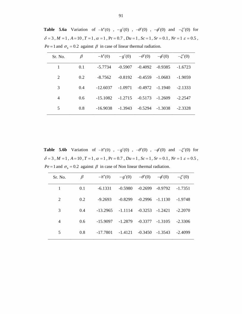
91
Table 5.6a Variation of (0)h′′− , (0)g ′− , (0)θ ′− , (0)φ′− and (0)ξ ′− for
3δ = , 1M = , 10A = , 1T = , 1α = , Pr 0.7= , 1Du = , 1Sc = , 0.1Sr = , 1Nr = 0.5ε = ,
1Pe = and 0.2bσ = against β in case of linear thermal radiation.
Sr. No. β (0)h′′− (0)g ′− (0)θ ′− (0)φ′− (0)ξ ′−
1 0.1 -5.7734 -0.5907 -0.4092 -0.9385 -1.6723
2 0.2 -8.7562 -0.8192 -0.4559 -1.0683 -1.9059
3 0.4 -12.6037 -1.0971 -0.4972 -1.1940 -2.1333
4 0.6 -15.1082 -1.2715 -0.5173 -1.2609 -2.2547
5 0.8 -16.9038 -1.3943 -0.5294 -1.3038 -2.3328
Table 5.6b Variation of (0)h′′− , (0)g ′− , (0)θ ′− , (0)φ′− and (0)ξ ′− for
3δ = , 1M = , 10A = , 1T = , 1α = , Pr 0.7= , 1Du = , 1Sc = , 0.1Sr = , 1Nr = 0.5ε = ,
1Pe = and 0.2bσ = against β in case of Non linear thermal radiation.
Sr. No. β (0)h′′− (0)g ′− (0)θ ′− (0)φ′− (0)ξ ′−
1 0.1 -6.1331 -0.5980 -0.2699 -0.9792 -1.7351
2 0.2 -9.2693 -0.8299 -0.2996 -1.1130 -1.9748
3 0.4 -13.2965 -1.1114 -0.3253 -1.2421 -2.2070
4 0.6 -15.9097 -1.2879 -0.3377 -1.3105 -2.3306
5 0.8 -17.7801 -1.4121 -0.3450 -1.3543 -2.4099
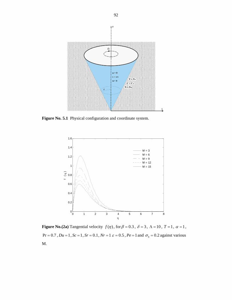
92
Figure No. 5.1 Physical configuration and coordinate system.
0 1 2 3 4 5 6 7 80
0.2
0.4
0.6
0.8
1
1.2
1.4
1.6
η
f
( η )
M = 3
M = 6
M = 9M = 12
M = 15
Figure No.(2a) Tangential velocity ( )f η , for 0.3β = , 3δ = , 10Λ = , 1T = , 1α = ,
Pr 0.7= , 1Du = , 1Sc = , 0.1Sr = , 1Nr = 0.5ε = , 1Pe = and 0.2bσ = against various
M.

93
0 1 2 3 4 5 6 7 80
0.2
0.4
0.6
0.8
1
1.2
1.4
1.6
η
f
( η )
M = 3
M = 6
M = 9M = 12
M = 15
Figure No. (2b) Tangential velocity ( )f η , for 0.3β = , 3δ = , 10Λ = , 1T = , 1α = ,
Pr 0.7= , 1Du = , 1Sc = , 0.1Sr = , 1Nr = 0.5ε = , 1Pe = and 0.2bσ = against various
M.
0 0.5 1 1.5 2 2.5 3 3.5 4 4.5 50
0.1
0.2
0.3
0.4
0.5
0.6
0.7
0.8
0.9
1
η
g (
η )
M = 3
M = 6
M = 9M = 12
M = 15
Figure No.(3a) Circumferential velocity ( )g η , for 0.3β = , 3δ = , 10Λ = , 1T = ,
1α = ,Pr 0.7= , 1Du = , 1Sc = , 0.1Sr = , 1Nr = 0.5ε = , 1Pe = and 0.2bσ = against
various M.
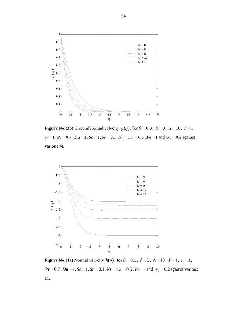
94
0 0.5 1 1.5 2 2.5 3 3.5 4 4.5 50
0.1
0.2
0.3
0.4
0.5
0.6
0.7
0.8
0.9
1
η
g (
η )
M = 3
M = 6
M = 9M = 12
M = 15
Figure No.(3b) Circumferential velocity ( )g η , for 0.3β = , 3δ = , 10Λ = , 1T = ,
1α = ,Pr 0.7= , 1Du = , 1Sc = , 0.1Sr = , 1Nr = 0.5ε = , 1Pe = and 0.2bσ = against
various M.
0 1 2 3 4 5 6 7 8 9 10-4.5
-4
-3.5
-3
-2.5
-2
-1.5
-1
-0.5
0
η
h (
η )
M = 3
M = 6
M = 9M = 12
M = 15
Figure No.(4a) Normal velocity ( )h η , for 0.3β = , 3δ = , 10Λ = , 1T = , 1α = ,
Pr 0.7= , 1Du = , 1Sc = , 0.1Sr = , 1Nr = 0.5ε = , 1Pe = and 0.2bσ = against various
M.
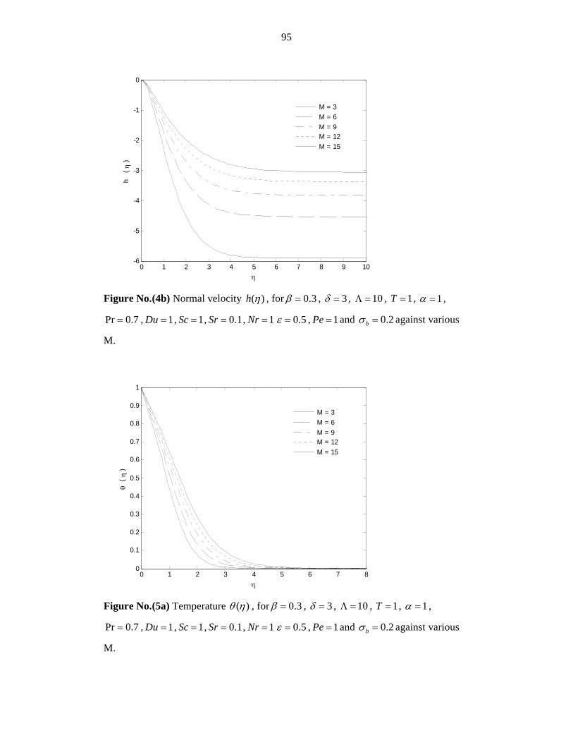
95
0 1 2 3 4 5 6 7 8 9 10-6
-5
-4
-3
-2
-1
0
η
h
( η
)
M = 3
M = 6
M = 9M = 12
M = 15
Figure No.(4b) Normal velocity ( )h η , for 0.3β = , 3δ = , 10Λ = , 1T = , 1α = ,
Pr 0.7= , 1Du = , 1Sc = , 0.1Sr = , 1Nr = 0.5ε = , 1Pe = and 0.2bσ = against various
M.
0 1 2 3 4 5 6 7 80
0.1
0.2
0.3
0.4
0.5
0.6
0.7
0.8
0.9
1
η
θ (
η )
M = 3
M = 6
M = 9M = 12
M = 15
Figure No.(5a) Temperature ( )θ η , for 0.3β = , 3δ = , 10Λ = , 1T = , 1α = ,
Pr 0.7= , 1Du = , 1Sc = , 0.1Sr = , 1Nr = 0.5ε = , 1Pe = and 0.2bσ = against various
M.

96
0 1 2 3 4 5 6 7 80
0.1
0.2
0.3
0.4
0.5
0.6
0.7
0.8
0.9
1
η
θ (
η )
M = 3
M = 6
M = 9M = 12
M = 15
Figure No.(5b) Temperature ( )θ η , for 0.3β = , 3δ = , 10Λ = , 1T = , 1α = ,
Pr 0.7= , 1Du = , 1Sc = , 0.1Sr = , 1Nr = 0.5ε = , 1Pe = and 0.2bσ = against various
M.
0 1 2 3 4 5 60
0.1
0.2
0.3
0.4
0.5
0.6
0.7
0.8
0.9
1
η
φ (
η )
M = 3
M = 6
M = 9M = 12
M = 15
Figure No.(6a) Concentration ( )φ η , for 0.3β = , 3δ = , 10Λ = , 1T = , 1α = ,
Pr 0.7= , 1Du = , 1Sc = , 0.1Sr = , 1Nr = 0.5ε = , 1Pe = and 0.2bσ = against various
M.

97
0 1 2 3 4 5 60
0.1
0.2
0.3
0.4
0.5
0.6
0.7
0.8
0.9
1
η
φ (
η )
M = 3
M = 6
M = 9M = 12
M = 15
Figure No.(6b) Concentration ( )φ η , for 0.3β = , 3δ = , 10Λ = , 1T = , 1α = ,
Pr 0.7= , 1Du = , 1Sc = , 0.1Sr = , 1Nr = 0.5ε = , 1Pe = and 0.2bσ = against various
M.
0 0.5 1 1.5 2 2.5 30
0.2
0.4
0.6
0.8
1
η
ξ (
η )
M = 3
M = 6
M = 9M = 12
M = 15
Figure No.(7a) Concentration of motile micro organisms( )ζ η , for 0.3β = , 3δ = ,
10Λ = , 1T = , 1α = , Pr 0.7= , 1Du = , 1Sc = , 0.1Sr = , 1Nr = 0.5ε = , 1Pe = and
0.2bσ = against various M.

98
0 0.5 1 1.5 2 2.5 30
0.2
0.4
0.6
0.8
1
η
ξ (
η )
M = 3
M = 6
M = 9M = 12
M = 15
Figure No.(7b) Concentration of motile micro organisms( )ζ η , for 0.3β = , 3δ = ,
10Λ = , 1T = , 1α = , Pr 0.7= , 1Du = , 1Sc = , 0.1Sr = , 1Nr = 0.5ε = , 1Pe = and
0.2bσ = against various M.
0 1 2 3 4 5 6 7 80
0.5
1
1.5
2
2.5
3
η
f
( η )
δ = 2
δ = 4
δ = 6
δ = 8
δ = 10
Figure No.(8a) Tangential velocity ( )f η , for 0.3β = , 1M = , 10Λ = , 1T = ,
1α = ,Pr 0.7= , 1Du = , 1Sc = , 0.1Sr = , 1Nr = 0.5ε = , 1Pe = and 0.2bσ = against
various δ .
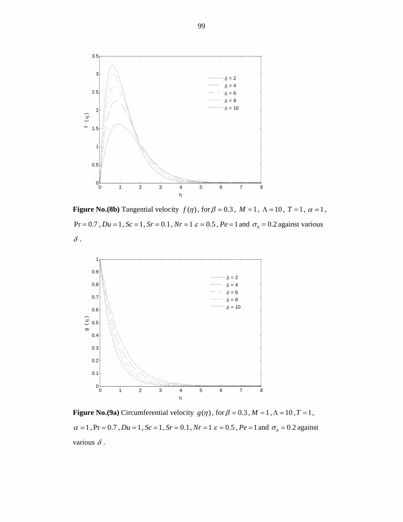
99
0 1 2 3 4 5 6 7 80
0.5
1
1.5
2
2.5
3
3.5
η
f
( η )
δ = 2
δ = 4
δ = 6
δ = 8
δ = 10
Figure No.(8b) Tangential velocity ( )f η , for 0.3β = , 1M = , 10Λ = , 1T = , 1α = ,
Pr 0.7= , 1Du = , 1Sc = , 0.1Sr = , 1Nr = 0.5ε = , 1Pe = and 0.2bσ = against various
δ .
0 1 2 3 4 5 6 7 80
0.1
0.2
0.3
0.4
0.5
0.6
0.7
0.8
0.9
1
η
g (
η )
δ = 2
δ = 4
δ = 6
δ = 8
δ = 10
Figure No.(9a) Circumferential velocity ( )g η , for 0.3β = , 1M = , 10Λ = , 1T = ,
1α = ,Pr 0.7= , 1Du = , 1Sc = , 0.1Sr = , 1Nr = 0.5ε = , 1Pe = and 0.2bσ = against
various δ .

100
0 1 2 3 4 5 6 7 80
0.1
0.2
0.3
0.4
0.5
0.6
0.7
0.8
0.9
1
η
g (
η )
δ = 2
δ = 4
δ = 6
δ = 8
δ = 10
Figure No.(9b) Circumferential velocity ( )g η , for 0.3β = , 1M = , 10Λ = , 1T = ,
1α = ,Pr 0.7= , 1Du = , 1Sc = , 0.1Sr = , 1Nr = 0.5ε = , 1Pe = and 0.2bσ = against
various δ .
0 1 2 3 4 5 6 7 8 9 10-7
-6
-5
-4
-3
-2
-1
0
η
h (
η )
δ = 2
δ = 4
δ = 6
δ = 8
δ = 10
Figure No.(10a) Normal velocity ( )h η , for 0.3β = , 1M = , 10Λ = , 1T = ,
1α = ,Pr 0.7= , 1Du = , 1Sc = , 0.1Sr = , 1Nr = 0.5ε = , 1Pe = and 0.2bσ = against
various δ .

101
0 1 2 3 4 5 6 7 8 9 10-12
-10
-8
-6
-4
-2
0
η
h
( η
)
δ = 2
δ = 4
δ = 6
δ = 8
δ = 10
Figure No.(10b) Normal velocity ( )h η , for 0.3β = , 1M = , 10Λ = , 1T = , 1α = ,
Pr 0.7= , 1Du = , 1Sc = , 0.1Sr = , 1Nr = 0.5ε = , 1Pe = and 0.2bσ = against various
δ .
0 0.5 1 1.5 2 2.5 3 3.5 40
0.1
0.2
0.3
0.4
0.5
0.6
0.7
0.8
0.9
1
η
θ (
η )
δ = 2
δ = 4
δ = 6
δ = 8
δ = 10
Figure No.(11a) Temperature ( )θ η , for 0.3β = , 1M = , 10Λ = , 1T = , 1α = ,
Pr 0.7= , 1Du = , 1Sc = , 0.1Sr = , 1Nr = 0.5ε = , 1Pe = and 0.2bσ = against various
δ .
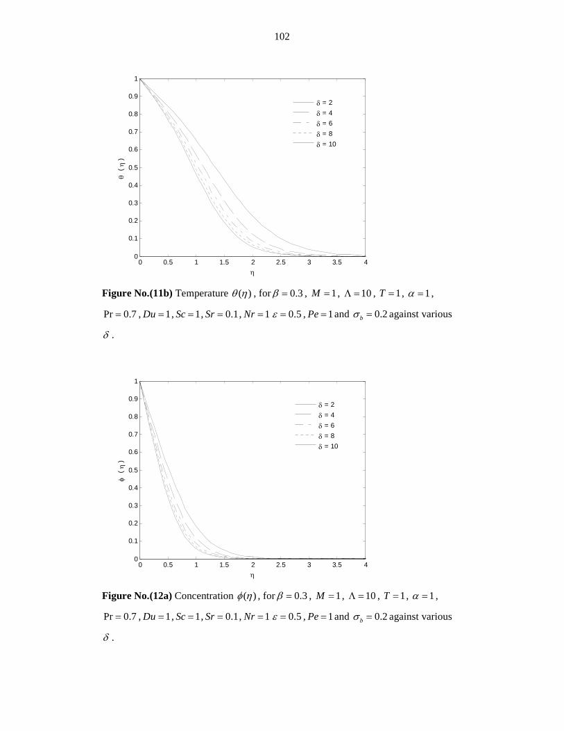
102
0 0.5 1 1.5 2 2.5 3 3.5 40
0.1
0.2
0.3
0.4
0.5
0.6
0.7
0.8
0.9
1
η
θ (
η )
δ = 2
δ = 4
δ = 6
δ = 8
δ = 10
Figure No.(11b) Temperature ( )θ η , for 0.3β = , 1M = , 10Λ = , 1T = , 1α = ,
Pr 0.7= , 1Du = , 1Sc = , 0.1Sr = , 1Nr = 0.5ε = , 1Pe = and 0.2bσ = against various
δ .
0 0.5 1 1.5 2 2.5 3 3.5 40
0.1
0.2
0.3
0.4
0.5
0.6
0.7
0.8
0.9
1
η
φ
( η
)
δ = 2
δ = 4
δ = 6
δ = 8
δ = 10
Figure No.(12a) Concentration ( )φ η , for 0.3β = , 1M = , 10Λ = , 1T = , 1α = ,
Pr 0.7= , 1Du = , 1Sc = , 0.1Sr = , 1Nr = 0.5ε = , 1Pe = and 0.2bσ = against various
δ .

103
0 0.5 1 1.5 2 2.5 3 3.5 40
0.1
0.2
0.3
0.4
0.5
0.6
0.7
0.8
0.9
1
η
φ
( η
)
δ = 2
δ = 4
δ = 6
δ = 8
δ = 10
Figure No.(12b) Concentration ( )φ η , for 0.3β = , 1M = , 10Λ = , 1T = , 1α = ,
Pr 0.7= , 1Du = , 1Sc = , 0.1Sr = , 1Nr = 0.5ε = , 1Pe = and 0.2bσ = against various
δ .
0 0.5 1 1.5 2 2.5 30
0.2
0.4
0.6
0.8
1
η
ξ (
η )
δ = 2
δ = 4
δ = 6
δ = 8
δ = 10
Figure No.(13a) Concentration of motile micro organisms( )ζ η , for 0.3β = , 1M = ,
10Λ = , 1T = , 1α = , Pr 0.7= , 1Du = , 1Sc = , 0.1Sr = , 1Nr = 0.5ε = , 1Pe = and
0.2bσ = against various δ .
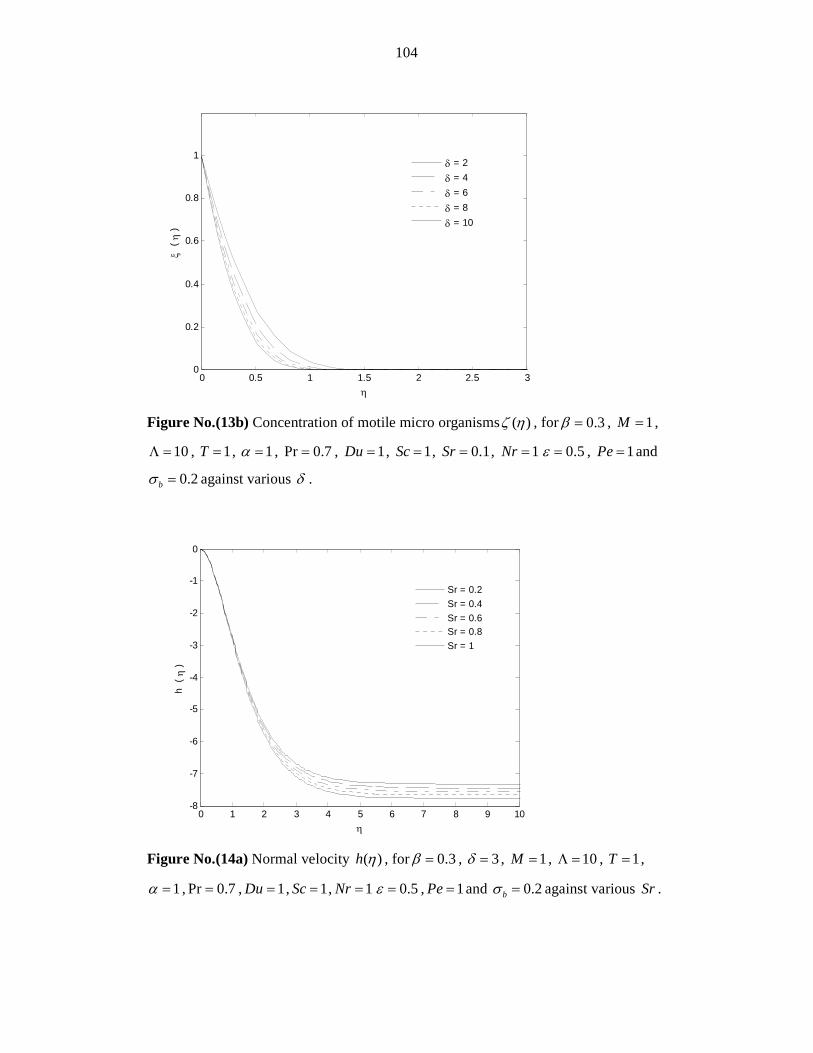
104
0 0.5 1 1.5 2 2.5 30
0.2
0.4
0.6
0.8
1
η
ξ (
η )
δ = 2
δ = 4
δ = 6
δ = 8
δ = 10
Figure No.(13b) Concentration of motile micro organisms( )ζ η , for 0.3β = , 1M = ,
10Λ = , 1T = , 1α = , Pr 0.7= , 1Du = , 1Sc = , 0.1Sr = , 1Nr = 0.5ε = , 1Pe = and
0.2bσ = against various δ .
0 1 2 3 4 5 6 7 8 9 10-8
-7
-6
-5
-4
-3
-2
-1
0
η
h (
η )
Sr = 0.2
Sr = 0.4
Sr = 0.6Sr = 0.8
Sr = 1
Figure No.(14a) Normal velocity ( )h η , for 0.3β = , 3δ = , 1M = , 10Λ = , 1T = ,
1α = ,Pr 0.7= , 1Du = , 1Sc = , 1Nr = 0.5ε = , 1Pe = and 0.2bσ = against various Sr .

105
0 1 2 3 4 5 6 7 8 9 10-9
-8
-7
-6
-5
-4
-3
-2
-1
0
η
h
( η
)
Sr = 0.2
Sr = 0.4
Sr = 0.6Sr = 0.8
Sr = 1
Figure No.(14b) Normal velocity ( )h η , for 0.3β = , 3δ = , 1M = , 10Λ = , 1T = ,
1α = ,Pr 0.7= , 1Du = , 1Sc = , 1Nr = 0.5ε = , 1Pe = and 0.2bσ = against various Sr .
0 0.5 1 1.5 2 2.5 3 3.5 40
0.1
0.2
0.3
0.4
0.5
0.6
0.7
0.8
0.9
1
η
φ (
η )
Sr = 0.2
Sr = 0.4
Sr = 0.6Sr = 0.8
Sr = 1
Figure No.(15a) Concentration ( )φ η , for 0.3β = , 3δ = , 1M = , 10Λ = , 1T = ,
1α = ,Pr 0.7= , 1Du = , 1Sc = , 1Nr = 0.5ε = , 1Pe = and 0.2bσ = against various Sr .

106
0 0.5 1 1.5 2 2.5 3 3.5 40
0.1
0.2
0.3
0.4
0.5
0.6
0.7
0.8
0.9
1
η
φ (
η )
Sr = 0.2
Sr = 0.4
Sr = 0.6Sr = 0.8
Sr = 1
Figure No.(15b) Concentration ( )φ η , for 0.3β = , 3δ = , 1M = , 10Λ = , 1T = ,
1α = ,Pr 0.7= , 1Du = , 1Sc = , 1Nr = 0.5ε = , 1Pe = and 0.2bσ = against various Sr .
0 1 2 3 4 5 6 7 80
0.5
1
1.5
2
2.5
η
f
( η )
Du = 1
Du = 2
Du = 3Du = 4
Du = 5
Figure No.(16a) Tangential velocity ( )f η , for 0.3β = , 3δ = , 1M = , 10Λ = , 1T = ,
1α = ,Pr 0.7= , 1Sc = , 0.1Sr = , 1Nr = 0.5ε = , 1Pe = and 0.2bσ = against various
Du .

107
0 1 2 3 4 5 6 7 80
0.5
1
1.5
2
2.5
η
f
( η )
Du = 1
Du = 2
Du = 3Du = 4
Du = 5
Figure No.(16b) Tangential velocity ( )f η , for 0.3β = , 3δ = , 1M = , 10Λ = , 1T = ,
1α = ,Pr 0.7= , 1Sc = , 0.1Sr = , 1Nr = 0.5ε = , 1Pe = and 0.2bσ = against various
Du .
0 1 2 3 4 5 6 7 8 9 10-9
-8
-7
-6
-5
-4
-3
-2
-1
0
1
η
h (
η )
Du = 1
Du = 2
Du = 3Du = 4
Du = 5
Figure No.(17a) Normal velocity ( )h η , for 0.3β = , 3δ = , 1M = , 10Λ = , 1T = ,
1α = ,Pr 0.7= , 1Sc = , 0.1Sr = , 1Nr = 0.5ε = , 1Pe = and 0.2bσ = against various
Du .
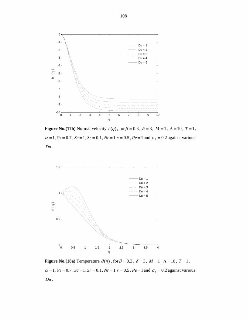
108
0 1 2 3 4 5 6 7 8 9 10-10
-9
-8
-7
-6
-5
-4
-3
-2
-1
0
η
h
( η
)
Du = 1
Du = 2
Du = 3Du = 4
Du = 5
Figure No.(17b) Normal velocity ( )h η , for 0.3β = , 3δ = , 1M = , 10Λ = , 1T = ,
1α = ,Pr 0.7= , 1Sc = , 0.1Sr = , 1Nr = 0.5ε = , 1Pe = and 0.2bσ = against various
Du .
0 0.5 1 1.5 2 2.5 3 3.5 40
0.5
1
1.5
η
θ (
η )
Du = 1
Du = 2
Du = 3Du = 4
Du = 5
Figure No.(18a) Temperature ( )θ η , for 0.3β = , 3δ = , 1M = , 10Λ = , 1T = ,
1α = ,Pr 0.7= , 1Sc = , 0.1Sr = , 1Nr = 0.5ε = , 1Pe = and 0.2bσ = against various
Du .

109
0 0.5 1 1.5 2 2.5 3 3.5 40
0.5
1
1.5
η
θ (
η )
Du = 1
Du = 2
Du = 3Du = 4
Du = 5
Figure No.(18b) Temperature ( )θ η , for 0.3β = , 3δ = , 1M = , 10Λ = , 1T = ,
1α = ,Pr 0.7= , 1Sc = , 0.1Sr = , 1Nr = 0.5ε = , 1Pe = and 0.2bσ = against various
Du .
0 1 2 3 4 5 6 7 80
0.5
1
1.5
2
2.5
η
f
( η )
∧ = 5
∧ = 10
∧ = 15
∧ = 20
∧ = 25
Figure No.(19a) Tangential velocity ( )f η , for 0.3β = , 3δ = , 1M = , 1T = , 1α = ,
Pr 0.7= , 1Du = , 1Sc = , 0.1Sr = , 1Nr = 0.5ε = , 1Pe = and 0.2bσ = against various
Λ .

110
0 1 2 3 4 5 6 7 80
0.5
1
1.5
2
2.5
3
η
f
( η )
∧ = 5
∧ = 10
∧ = 15
∧ = 20
∧ = 25
Figure No.(19b) Tangential velocity ( )f η , for 0.3β = , 3δ = , 1M = , 1T = , 1α = ,
Pr 0.7= , 1Du = , 1Sc = , 0.1Sr = , 1Nr = 0.5ε = , 1Pe = and 0.2bσ = against various
Λ .
0 1 2 3 4 5 60
0.1
0.2
0.3
0.4
0.5
0.6
0.7
0.8
0.9
1
η
g (
η )
∧ = 5
∧ = 10
∧ = 15
∧ = 20
∧ = 25
Figure No.(20a) Circumferential velocity ( )g η , for 0.3β = , 3δ = , 1M = , 1T = ,
1α = ,Pr 0.7= , 1Du = , 1Sc = , 0.1Sr = , 1Nr = 0.5ε = , 1Pe = and 0.2bσ = against
various Λ .

111
0 1 2 3 4 5 60
0.1
0.2
0.3
0.4
0.5
0.6
0.7
0.8
0.9
1
η
g (
η )
∧ = 5
∧ = 10
∧ = 15
∧ = 20
∧ = 25
Figure No.(20b) Circumferential velocity ( )g η , for 0.3β = , 3δ = , 1M = , 1T = ,
1α = ,Pr 0.7= , 1Du = , 1Sc = , 0.1Sr = , 1Nr = 0.5ε = , 1Pe = and 0.2bσ = against
various Λ .
0 1 2 3 4 5 6 7 8 9 10-9
-8
-7
-6
-5
-4
-3
-2
-1
0
η
h (
η )
∧ = 5
∧ = 10
∧ = 15
∧ = 20
∧ = 25
Figure No.(21a) Normal velocity ( )h η , for 0.3β = , 3δ = , 1M = , 1T = , 1α = ,
Pr 0.7= , 1Du = , 1Sc = , 0.1Sr = , 1Nr = 0.5ε = , 1Pe = and 0.2bσ = against various
Λ .

112
0 1 2 3 4 5 6 7 8 9 10-11
-10
-9
-8
-7
-6
-5
-4
-3
-2
-1
0
η
h
( η
)
∧ = 5
∧ = 10
∧ = 15
∧ = 20
∧ = 25
Figure No.(21b) Normal velocity ( )h η , for 0.3β = , 3δ = , 1M = , 1T = , 1α = ,
Pr 0.7= , 1Du = , 1Sc = , 0.1Sr = , 1Nr = 0.5ε = , 1Pe = and 0.2bσ = against various
Λ .
0 1 2 3 4 5 60
0.1
0.2
0.3
0.4
0.5
0.6
0.7
0.8
0.9
1
η
θ (
η )
∧ = 5
∧ = 10
∧ = 15
∧ = 20
∧ = 25
Figure No.(22a) Temperature ( )θ η , for 0.3β = , 3δ = , 1M = , 1T = , 1α = ,
Pr 0.7= , 1Du = , 1Sc = , 0.1Sr = , 1Nr = 0.5ε = , 1Pe = and 0.2bσ = against various
Λ .

113
0 1 2 3 4 5 60
0.1
0.2
0.3
0.4
0.5
0.6
0.7
0.8
0.9
1
η
θ (
η )
∧ = 5
∧ = 10
∧ = 15
∧ = 20
∧ = 25
Figure No.(22b) Temperature ( )θ η , for 0.3β = , 3δ = , 1M = , 1T = , 1α = ,
Pr 0.7= , 1Du = , 1Sc = , 0.1Sr = , 1Nr = 0.5ε = , 1Pe = and 0.2bσ = against various
Λ .
0 0.5 1 1.5 2 2.5 3 3.5 40
0.1
0.2
0.3
0.4
0.5
0.6
0.7
0.8
0.9
1
η
φ (
η )
∧ = 5
∧ = 10
∧ = 15
∧ = 20
∧ = 25
Figure No.(23a) Concentration ( )φ η , for 0.3β = , 3δ = , 1M = , 1T = , 1α = ,
Pr 0.7= , 1Du = , 1Sc = , 0.1Sr = , 1Nr = 0.5ε = , 1Pe = and 0.2bσ = against various
Λ .
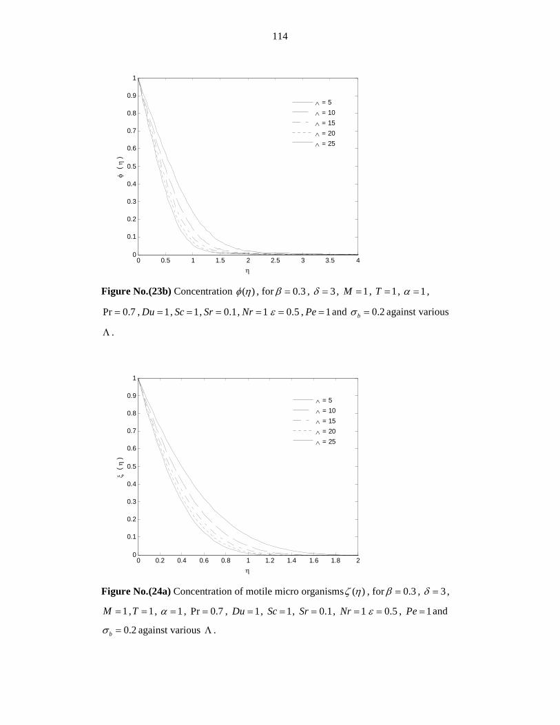
114
0 0.5 1 1.5 2 2.5 3 3.5 40
0.1
0.2
0.3
0.4
0.5
0.6
0.7
0.8
0.9
1
η
φ (
η )
∧ = 5
∧ = 10
∧ = 15
∧ = 20
∧ = 25
Figure No.(23b) Concentration ( )φ η , for 0.3β = , 3δ = , 1M = , 1T = , 1α = ,
Pr 0.7= , 1Du = , 1Sc = , 0.1Sr = , 1Nr = 0.5ε = , 1Pe = and 0.2bσ = against various
Λ .
0 0.2 0.4 0.6 0.8 1 1.2 1.4 1.6 1.8 20
0.1
0.2
0.3
0.4
0.5
0.6
0.7
0.8
0.9
1
η
ξ (
η )
∧ = 5
∧ = 10
∧ = 15
∧ = 20
∧ = 25
Figure No.(24a) Concentration of motile micro organisms( )ζ η , for 0.3β = , 3δ = ,
1M = , 1T = , 1α = , Pr 0.7= , 1Du = , 1Sc = , 0.1Sr = , 1Nr = 0.5ε = , 1Pe = and
0.2bσ = against various Λ .

115
0 0.2 0.4 0.6 0.8 1 1.2 1.4 1.6 1.8 20
0.1
0.2
0.3
0.4
0.5
0.6
0.7
0.8
0.9
1
η
ξ (
η )
∧ = 5
∧ = 10
∧ = 15
∧ = 20
∧ = 25
Figure No.(24b) Concentration of motile micro organisms( )ζ η , for 0.3β = , 3δ = ,
1M = , 1T = , 1α = , Pr 0.7= , 1Du = , 1Sc = , 0.1Sr = , 1Nr = 0.5ε = , 1Pe = and
0.2bσ = against various Λ .
0 1 2 3 4 5 6 7 8 9 100
0.2
0.4
0.6
0.8
1
1.2
1.4
1.6
1.8
2
η
f
( η )
β = 0.1
β = 0.2
β = 0.4
β = 0.6
β = 0.8
Figure No.(25a) Tangential velocity ( )f η , for 3δ = , 1M = , 10Λ = , 1T = , 1α = ,
Pr 0.7= , 1Du = , 1Sc = , 0.1Sr = , 1Nr = 0.5ε = , 1Pe = and 0.2bσ = against various
β .

116
0 1 2 3 4 5 6 7 8 9 100
0.5
1
1.5
2
2.5
η
f
( η )
β = 0.1
β = 0.2
β = 0.4
β = 0.6
β = 0.8
Figure No.(25b) Tangential velocity ( )f η , for 3δ = , 1M = , 10Λ = , 1T = , 1α = ,
Pr 0.7= , 1Du = , 1Sc = , 0.1Sr = , 1Nr = 0.5ε = , 1Pe = and 0.2bσ = against various
β .
0 1 2 3 4 5 6 7 8 9 100
0.1
0.2
0.3
0.4
0.5
0.6
0.7
0.8
0.9
1
η
g (
η )
β = 0.1
β = 0.2
β = 0.4
β = 0.6
β = 0.8
Figure No.(26a) Circumferential velocity ( )g η , for 3δ = , 1M = , 10Λ = , 1T = ,
1α = ,Pr 0.7= , 1Du = , 1Sc = , 0.1Sr = , 1Nr = 0.5ε = , 1Pe = and 0.2bσ = against
various β .

117
0 1 2 3 4 5 6 7 8 9 100
0.1
0.2
0.3
0.4
0.5
0.6
0.7
0.8
0.9
1
η
g (
η )
β = 0.1
β = 0.2
β = 0.4
β = 0.6
β = 0.8
Figure No.(26b) Circumferential velocity ( )g η , for 3δ = , 1M = , 10Λ = , 1T = ,
1α = ,Pr 0.7= , 1Du = , 1Sc = , 0.1Sr = , 1Nr = 0.5ε = , 1Pe = and 0.2bσ = against
various β .
0 1 2 3 4 5 6 7 8 9 10-7
-6
-5
-4
-3
-2
-1
0
η
h (
η )
β = 0.1
β = 0.2
β = 0.4
β = 0.6
β = 0.8
Figure No.(27a) Normal velocity ( )h η , for 3δ = , 1M = , 10Λ = , 1T = , 1α = ,
Pr 0.7= , 1Du = , 1Sc = , 0.1Sr = , 1Nr = 0.5ε = , 1Pe = and 0.2bσ = against various
β .

118
0 1 2 3 4 5 6 7 8 9 10-9
-8
-7
-6
-5
-4
-3
-2
-1
0
η
h
( η
)
β = 0.1
β = 0.2
β = 0.4
β = 0.6
β = 0.8
Figure No.(27b) Normal velocity ( )h η , for 3δ = , 1M = , 10Λ = , 1T = , 1α = ,
Pr 0.7= , 1Du = , 1Sc = , 0.1Sr = , 1Nr = 0.5ε = , 1Pe = and 0.2bσ = against various
β .
0 0.5 1 1.5 2 2.5 3 3.5 40
0.1
0.2
0.3
0.4
0.5
0.6
0.7
0.8
0.9
1
η
θ (
η )
β = 0.1
β = 0.2
β = 0.4
β = 0.6
β = 0.8
Figure No.(28a) Temperature ( )θ η , for 3δ = , 1M = , 10Λ = , 1T = , 1α = ,
Pr 0.7= , 1Du = , 1Sc = , 0.1Sr = , 1Nr = 0.5ε = , 1Pe = and 0.2bσ = against various
β .

119
0 0.5 1 1.5 2 2.5 3 3.5 40
0.1
0.2
0.3
0.4
0.5
0.6
0.7
0.8
0.9
1
η
θ (
η )
β = 0.1
β = 0.2
β = 0.4
β = 0.6
β = 0.8
Figure No.(28b) Temperature ( )θ η , for 3δ = , 1M = , 10Λ = , 1T = , 1α = ,
Pr 0.7= , 1Du = , 1Sc = , 0.1Sr = , 1Nr = 0.5ε = , 1Pe = and 0.2bσ = against various
β .
0 0.5 1 1.5 2 2.5 3 3.5 40
0.1
0.2
0.3
0.4
0.5
0.6
0.7
0.8
0.9
1
η
φ
( η
)
β = 0.1
β = 0.2
β = 0.4
β = 0.6
β = 0.8
Figure No.(29a) Concentration ( )φ η , for 3δ = , 1M = , 10Λ = , 1T = , 1α = ,
Pr 0.7= , 1Du = , 1Sc = , 0.1Sr = , 1Nr = 0.5ε = , 1Pe = and 0.2bσ = against various
β .

120
0 0.5 1 1.5 2 2.5 3 3.5 40
0.1
0.2
0.3
0.4
0.5
0.6
0.7
0.8
0.9
1
η
φ
( η
)
β = 0.1
β = 0.2
β = 0.4
β = 0.6
β = 0.8
Figure No. 29(b) Concentration ( )φ η , for 3δ = , 1M = , 10Λ = , 1T = , 1α = ,
Pr 0.7= , 1Du = , 1Sc = , 0.1Sr = , 1Nr = 0.5ε = , 1Pe = and 0.2bσ = against various
β .
0 0.2 0.4 0.6 0.8 1 1.2 1.4 1.6 1.8 20
0.1
0.2
0.3
0.4
0.5
0.6
0.7
0.8
0.9
1
η
ξ (
η )
β = 0.1
β = 0.2
β = 0.4
β = 0.6
β = 0.8
Figure No.30(a) Concentration of motile micro organisms( )ζ η , for 3δ = , 1M = ,
10Λ = , 1T = , 1α = , Pr 0.7= , 1Du = , 1Sc = , 0.1Sr = , 1Nr = 0.5ε = , 1Pe = and
0.2bσ = against various β .

121
0 0.2 0.4 0.6 0.8 1 1.2 1.4 1.6 1.8 20
0.1
0.2
0.3
0.4
0.5
0.6
0.7
0.8
0.9
1
η
ξ (
η )
β = 0.1
β = 0.2
β = 0.4
β = 0.6
β = 0.8
Figure No. 30(b) Concentration of motile micro organisms( )ζ η , for 3δ = , 1M = ,
10Λ = , 1T = , 1α = , Pr 0.7= , 1Du = , 1Sc = , 0.1Sr = , 1Nr = 0.5ε = , 1Pe = and
0.2bσ = against various β .

122
POSSIBLE FUTURE WORK
In the chapter 2, we presented the numerical solution of the flow, heat and
concentration of an incompressible and electrically conducting nano-fluid
between the two permeable coaxial disks which move orthogonally, the nano-
particles 2TiO are inserted in the base fluid. The flow is laminar and unsteady.
The Joule heating and viscous dissipation are taken into account. The study
undertaken in the chapter 2 is intended to extend to the non-symmetric case
when one disk is porous while the other is non porous. We may further consider
the mass transfer of a chemically reactive species between the two disks. The
nano-fluid may be assumed to contain some chemically reactive species, and the
mixture thus formed is homogeneous. Moreover, 1st order homogeneous and
irreversible reaction may also assumed to be taking place in the fluid because of
chemical reactive nature of the species. The numerical investigation of the
problem of the flow, heat and concentration of an electrically conduction nano-
fluid through a semi-infinite open ended porous channel is carried out in
chapter 3 may be extended to the case of endothermic exothermic chemical
reactions. Physical characteristics of the momentum and thermal aspects of the
problem may be explored by analyzing the fluid velocity, temperature profile,
the skin-friction coefficient, couple wall stress and the local Nusselt number.
In chapter 4, we discussed the flow and heat transfer in 2-dimensional
steady and incompressible Casson fluid flow over a circular coiled curved
stretching sheet. The curved sheet is stretched with the fixed origin, due to the
action of two forces (equal in the magnitude but opposite in the direction). The
fluid has the property of electrical conduction and magnetic field. The magnetic
Reynolds number is assumed really small with the intention that the induced
magnetic field can be ignored. The numerical scheme used in this chapter may
be extended for the numerical solution of the complete Navier-Stokes equations,
to study the mixed convection in an enclosure with heat flux from some parts of
its vertical walls. We have already developed the computer code for the problem

123
in the MATLAB environment. As a sample output, the stream function and
temperature distribution for the problem (for certain values of the governing
parameters) are given below.
0 0.1 0.2 0.3 0.4 0.5 0.6 0.7 0.8 0.9 10
0.1
0.2
0.3
0.4
0.5
0.6
0.7
0.8
0.9
1
Fig. 1 Streamlines when only top lid is moving with Re = 500.

124
0 0.1 0.2 0.3 0.4 0.5 0.6 0.7 0.8 0.9 10
0.1
0.2
0.3
0.4
0.5
0.6
0.7
0.8
0.9
1
Fig. 2 Streamlines when both lids are moving in the same direction with Re = 500.
0 0.1 0.2 0.3 0.4 0.5 0.6 0.7 0.8 0.9 10
0.1
0.2
0.3
0.4
0.5
0.6
0.7
0.8
0.9
1
Fig. 3 Streamlines when both lids are moving in the opposite direction with Re = 500.

125
In chapter 5, a comparative study has been carried out between linear and
nonlinear approaches of the Rosseland approximation for the thermal radiations
in the boundary layer flow of a Casson fluid over a vertically rotating cone.
We assumed the presence of an external magnetic field which was being
uniformly applied on the fluid, irrespective of its position w.r.t. the origin of the
coordinate system being used. In order to make the problem physically more
realistic, we intend to consider the spatially varying magnetic field. This will
remarkably alter the mathematical modeling of the problem, but the results thus
obtained will have more significant physical meanings. We have seen quite a
few references on this type of problems in different geometries.

126
LIST OF PUBLICATIONS
The contents of the thesis have led to the following papers which have been accepted / published
in international ISI indexed journals
1) Muhammad Farooq Iqbal, Kashif Ali and Muhammad Ashraf, 2014. Heat and mass
transfer analysis in unsteady titanium dioxide nanofluid between two orthogonally moving
porous coaxial disks-A numerical study. Canadian Journal of Physics (Canada), 93(3): 1-
10 (I.F=0.68).
2) Muhammad Farooq Iqbal, Shahzad Ahmad, Kashif Ali and Muhammad Ashraf, 2016.
Combined effect of heat and mass transfer in MHD flow of a nanofluid between
Expending/Contracting walls of a Porous Channel. Journal of Porous Media (USA), 19(9):
821-839 (I.F=1.05).
3) Muhammad Farooq Iqbal, Shazad Ahmad, Kashif Ali, M Zubair Akbar and M Ashraf,
2016. Heat and mass transfer analysis in unsteady nanofluid flow between moving disks with
chemical reaction-A numerical study. Heat Transfer Research (USA).
DOI: 10.1615/HeatTransRes.2018016244 (I.F=0.93)
4) Kashif Ali, Muhammad Zubair Akbar, Muhammad Farooq Iqbal and Muhammad Ashraf,
2014. Numerical simulation of heat and mass transfer in unsteady nanofluid between two
orthogonally moving porous coaxial disks. AIP Advances (USA), doi: 10.1063/1.4897947
(I.F=1.56).
5) Kashif Ali, Muhammad Farooq Iqbal, Muhammad Zubair Akbar and Muhammad Ashraf,
2014. Numerical simulation of unsteady water-based nanofluid flow and heat transfer
between two orthogonally moving porous coaxial disks. Journal of Theoretical and Applied
Mechanics (Poland), 52, 1033-1046 (I.F=0.68).
6) Muhammad Zubair Akbar, Muhammad Ashraf, Muhammad Farooq Iqbal, and Kashif Ali,
2016. Heat and mass transfer analysis of unsteady MHD nanofluid flow through a channel
with moving porous walls and medium. AIP Advances (USA) 6, doi.org/10.1063/1.4945440
(I.F=1.56).

127
7) M. Zubair Akbar Qureshi, Kashif Ali, Muhammad Farooq Iqbal, Muhammad Ashraf, and
Shazad Ahmad, 2017. Heat and mass transfer enhancement of nanofluids flow in thepresence
of metallic/metallic-oxides spherical nanoparticles. Eur. Phys. J. Plus, 132:57 (I.F=1.73).
8) M. Zubair Akbar Qureshi, Kashif Ali, Muhammad Farooq Iqbal and Muhammad Ashraf,
2017. Numerical modeling of non-newtonian fluid flow between porous disks in the presence
of nano particles. Nanoscience and Technology: AN International Journal (USA), 8(1), 67–
83 (I.F=0.0)
9) M Zubair Akbar, Kashif Ali, Muhammad Farooq Iqbal and M Ashraf, 2017. Heat and
mass transfer analysis of unsteady non-Newtonian fluid flow between porous surfaces in the
presence of magnetic nanoparticles. Journal of Porous Media (USA), 20(12):1137–1154
(I.F=1.05)

128
REFERENCES
[1] Von Karman T., (1921), Uber laminare and turbulente Reibung. Zeit. Angew. Math.
Mech., 1(4), 233–252.
[2] Cochran, W. G., (1934), The flow due to a rotating disk. Proc. Camb. Philo. Soc., 30(3),
365–375.
[3] Stewartson, K., (1953), On the flow between two rotating coaxial disks. Proc. Comb.
Phil. Soc., 49, 333–341.
[4] Chapple, P. J. and Stokes, V. K., (1962) On the flow between a rotating and a stationary
disk. Report No. FLD 8. Dept. Mech. Eng. Princeton University.
[5] Mellor, G. J., Chapple, P. J. and Stokes, V. K., (1968), On the flow between a rotating
and a stationary disk. J. FluidMech., 31, 95–112.
[6] Arora, R. C. and Stokes, V. K., (1972), On the heat transfer between two rotating disks.
Int. J. Heat Mass Transf.,15, 2119–2132.
[7] Yan, W. M. and Soong, C. Y., (1997), Mixed convection flow and heat transfer between
co-rotating porous disks with wall transpiration. Int. J. Heat Mass Transf., 40, 773–784.
[8] Soong, C. Y., Wu, C. C., Liu, T. P. and Liu, T. P., (2003), Flow structure between two
co-axial disks rotating independently. Exp. Thermal Fluid Sci., 27, 295–311.
[9] Domairry G. and Aziz, A., (2009), Approximate analysis of MHD squeeze flow
between two parallel disks with suction or injection by homotopy perturbation method.
Mathematical Problems in Engineering, 2009, 603916.
[10] Joneidi, A. A., Domairry, G. and Babaelahi, M., (2010), Effect of mass transfer on a flow
in the magnetohydrodynamic squeeze film between two parallel discs with one porous
disk. Chemical Engineering Communications, 198, 299–311.
[11] Hayat, T., Yousaf, A., Mustafa, M. and Obaidat, S., (2012), MHD squeezing flow of
second-grade fluid between two parallel disks. International Journal for Numerical
Methods in Fluids, 69, 399–410.
[12] Hussain, A., Mohyud-Din, S. T. and Cheema, T. A., (2012), Analytical and numerical
approaches to squeezing flow and heat transfer between two parallel disks with velocity
slip and temperature jump. Chinese Physics Letters, 29, 114705.
129
[13] Shaban, M., Shivanian, E. and Abbasbandy, S., (2013), Analyzing magnetohydrodynamic
squeezing flow between two parallel disks with suction or injection by a new hybrid
method based on the Tau method and the homotopy analysis method. European Physical
Journal Plus, 128, 1–10.
[14] Turkyilmazoglu, M., (2014), MHD fluid flow and heat transfer due to a shrinking
rotating disk. Compt. Fluid, 90, 51–56.
[15] Gao, Z. K., Fang, P. C. and Ding, MS, Jin, N. D., (2015), Multivariate weighted complex
network analysis for characterizing nonlinear dynamic behavior in two-phase flow. Exp.
Thermal Fluid Sci., 60, 157–164.
[16] Gao, Z. K., Yang, Y. X., Zhai, L. S. and Ding, MS, Jin, N. D., (2016), Characterizing
slug to churn flow transition by using multivariate pseudo Wigner distribution and
multivariate multiscale entropy. Chem. Eng. J., 291, 74–81.
[17] Gao, Z. K., Yang, Y., Zhai, L., Jin, N. and Chen, G., (2016), A four-sector conductance
method for measuring and characterizing low-velocity oil-water two-phase flows. IEEE
Trans. Instrumentation Measurement doi: 10.1109/TIM.2016.2540862 (in press).
[18] Gao, Z. K., Yang, Y. X., Fang, P. C., Jin, N., Xia, C. Y. and Hu, L. D., (2015), Multi-
frequency complex network from time series for uncovering oil-water flow structure.
Scientific Reports, 5, 8222.
[19] Makinde, O. D. and Aziz, A., (2011), Boundary layer flow of a nanofluid past a
stretching sheet with a convective boundary condition. International Journal
of Thermal Sciences, 50, 1326–1332.
[20] Bachok, N., Ishak, A., and Pop, I., (2012), Unsteady boundary-layer flow and heat
transfer of a nanofluid over a permeable stretching/shrinking sheet. International Journal
of Heat and Mass Transfer, 55, 2102–2109.
[21] Safaei, M. R., Togun, H., Vafai, K., Kazi, S. N., and Badarudin, A., (2014), Investigation
of heat transfer enhancement in a forward-facing contracting channel using FMWCNT
nanofluids. Numerical Heat Transfer Part A, 66, 1321–1340.
[22] Safaei, M. R., Mahian, O., Garoosi, F., Hooman, K., Karimipour, A., Kazi, S. N. and
Gharehkhani, S., (2014), Investigation of micro and nano-sized particle erosion in a 90°
pipe bend using a two-phase discrete phase model. Scientific World Journal, 2014,
740578.

130
[23] Goodarzi, M., Safaei, M. R., Vafai, K., Ahmadi, G., Dahari, M., Kazi, S. N., and
Jomhari, N., (2014), Investigation of nanofluid mixed convection in a shallow cavity
using a two-phase mixture model. International Journal of Thermal Sciences, 75, 204–
220.
[24] Togun, H., Safaei, M. R., Sadri, R., Kazi, S. N., Badarudin, A., Hooman, K., and
Sadeghinezhad, E., (2014), Numerical simulation of laminar to turbulent nanofluid flow
and heat transfer over a backward-facing step. Applied Mathematics and Computation,
239, 153–170.
[25] Hashmi, M. M., Hayat, T. and Alsaedi, A., (2012), On the analytic solutions for
squeezing flow of nanofluid between parallel disks. Nonlinear Anal Model
Control, 17, 418–430.
[26] Das, K., Jana, S. and Acharya, N., (2016), Slip effects on squeezing flow of nanofluid
between two parallel discs. International Journal of Applied Mechanics and Engineering,
21, 5–20.
[27] Lai, F. C. and Kulacki, F. A., (1990), The effect of variable viscosity on convective heat
transfer along a vertical surface in a saturated porous medium. International Journal of
Heat and Mass Transfer, 33, 1028–1031.
[28] Prasad, K. V., Vajravelu, K. and Vaidya, H., (2016), MHD Casson nanofluid flow and
heat transfer at a stretching sheet with variable thickness. Journal of Nanofluids, 5, 423–
435.
[29] Vajjha, R. S. and Das, D. K., (2012), A review and analysis on influence of temperature
and concentration of nanofluids on thermophysical properties, heat transfer and pumping
power. International Journal of Heat and Mass Transfer, 55, 4063–4078.
[30] Liao, S., (2003), Beyond perturbation: introduction to homotopy analysis method.
London: Chapman & Hall/CRC Press.
[31] Fan, T. and You, X., (2013), Optimal homotopy analysis method for nonlinear
differential equations in the boundary layer. Numerical Algorithms, 62, 337–354.
[32] Hayat, T., Imtiaz, M. and Alsaedi, A., (2015), MHD 3D flow of nanofluid in presence of
convective conditions. J. Mol. Liq., 212, 203–208.
131
[33] Sheikholeslami, M., Bandpy, M. G., Ganji, D. D. and Soleimani, S., (2013), Effect of a
magnetic field on natural convection in an inclined half-annulus enclosure filled with
Cu—water nanofluid using CVFEM. Adv. Powder Tech., 24, 980–991.22.
[34] Hsiao, K. L., (2016) Stagnation electrical MHD nanofluid mixed convection with slip
boundary on a stretching sheet. Appl. Therm. Eng., 98, 850–861.
[35] Hsiao, K. L., (2015), Corrigendum to Heat and mass mixed convection for MHD
viscoelastic fluid past a stretching sheet with Ohmic dissipation. Commu. Nonlinear Sci.
Numer. Simulate, 28, 232.
[36] Zhang, C., Zheng, L., Zhang, X. and Chen, G., (2015), MHD flow and radiation heat
transfer of nanofluids in porous media with variable surface heat flux and chemical
reaction. Appl. Math. Modeling, 39, 165–181.
[37] Ganji, D. D. and Malvandi, A., (2014), Natural convection of nanofluids inside a vertical
enclosure in the presence of a uniform magnetic field. Powder Tech., 263, 50–57.
[38] Hayat, T., Imtiaz, M., Alsaedi, A. and Mansoor, R., (2015), Magnetohydrodynamic three-
dimensional flow of nanofluid by a porous shrinking surface. J. Aerospace Eng., 29, (2),
doi: 10.1061/(ASCE)AS.1943-5525.0000533
[39] Yang, L. and Shen, H., (2015), Effects of the porous media distribution on the
performance improvement for isothermal chamber. Appl. Therm. Eng., 86, 301–308.
[40] Azimi, M. and Riazi, R., (2015), Heat transfer analysis of GO-water nanofluid flow
between two parallel disks. Propulsion and Power Research, 4, 23–30.
[41] Ganji, D. D., Abbasi, M., Rahimi., J., Gholami, M. and Rahimipetroudi, I., (2014), On
the MHD squeeze flow between two parallel disks with suction or injection via
HAM and HPM. Front Mech Eng, 9, 270–280.
[42] Hayat, T., Qayyum, A., Alsaadi, F., Awais, M. and Dobaie, A. M., (2013), Thermal
radiation effects in squeezing flow of a Jeffery fluid. Eur Phys J Plus, 128, 85.
[43] Domairry, G. and Aziz, A., (2009), Approximate analysis of MHD squeeze flow between
two parallel disks with suction or injection by homotopy perturbation
method. Math. Prob. Eng., 603916.
[44] Xin-hui, S. I., Lian-cun, ZHENG, Xin-xin, ZHANG and Xin-yi, S. I., (2012), Flow of
micropolar fluid between two orthogonally moving porous disks. Appl. Math. Mech. -
Engl. Ed., 33(8), 963–974.

132
[45] Sun Yina, Si Xinhui, Zheng Liancun, Shen Yanan and Zhang Xinxin, (2013), The
analysis of the flow of a micropolar fluid between two orthogonally moving porous disks
with counter rotating directions. Cent. Eur. J. Phys., 11(5), 601-614.
[46] Ingham, D. B., Pop, I. and Cheng, P., (1990), Combined free and forced convection
porous medium between two vertical walls with viscous dissipation. Transp. Porous
Media, 5, 381–398.
[47] Makinde, O. D. and Mhone, P. Y., (2005), Heat transfer to MHD oscillatory flow in a
channel filled with porous medium, Romanian J. Phys., 50, 931–938.
[48] Mehmood, A. and Ali, A., (2007), The effect of slip condition on unsteady MHD
oscillatory flow of a viscous fluid In a planer channel. Romanian J. Phys., 52, 85–91.
[49] Makinde, O. D. and Beg, O. A., (2010), On inherent irreversibility in a reactive
hydromagnetic channel flow. J. Therm. Sci., 19(1), 72–79.
[50] Jha, B. K. and Ajibade, A. O., (2010), Free convective flow between vertical porous
plates with periodic heat input. ZAMM Z. Angew. Math. Mech., 1–9,
http://dx.doi.org/10.1002/ zamm.200900268.
[51] Jha, B. K., Ajibade, A. O., (2009), Free convective flow of heat generating/ absorbing
fluid between vertical porous plates with periodic heat input. Int. Commun. Heat Mass
Transfer, 36, 624–631.
[52] Jha, B. K. and Ajibade, A. O., (2012), Effect of viscous dissipation on natural convection
flow between vertical parallel plates with timeperiodic boundary conditions. Commun.
Nonlinear Sci. Numer. Simul., 17, 1576–1587.
[53] Umavathi, J.C., (2011), Free convection of composite porous medium in a vertical
channel. Heat Transf. Asian Res., 40(4), 308–329.
[54] Srinivasacharya, D. and Kaladhar, K., (2013), Soret and Dufour effects on free
convection flow of a couple stress fluid in a vertical channel with chemical reaction.
Chem. Ind. Chem. Eng. Q., 19(1), 45–55.
[55] Garg, B.P., Singh, K.D. and Bansal, A.K., (2014), Hall current effect on viscoelastic
(Walters liquid model-B) MHD oscillatory convective channel flow through a porous
medium with heat radiation. Kragujev. J. Sci., 36, 19–32.

133
[56] Kothandapani, M. and Srinivas, S., (2008), Nonlinear peristaltic transport of a Newtonian
fluid in an inclined asymmetric channel through a porous medium. Phys Lett A 372,
1265–1276.
[57] Gnaneswara, Reddy, M., Venugopal, Reddy, K. and Makinde, O. D., (2016),
Hydromagnetic peristaltic motion of a reacting and radiatingcouple stress fluid in an
inclined asymmetric channel filled with a porous medium. Alex. Eng. J., 55, 1841–1853.
[58] Ali, N., Abbasi, A. and Ahmad, I., (2016), Channel flow of Ellis fluid due to
peristalsis. AIP Adv., 5, 097214. doi:10.1063/1.4932042
[59] Sarkar, B. C., Das, S., Jana, R. N. and Makinde, O. D., (2015), Magnetohydrodynamic
peristaltic flow of nanofluids in a convectively heated vertical asymmetric channel in
presence of thermal radiation. J. Nanofluids, 4, 461–473.
[60] Mekheimer, KhS. and Abd, Elmaboud, Y., (2015), Simultaneous effects of variable
viscosity and thermal conductivity on peristaltic flow in a vertical asymmetric channel.
Can. J. Phys., 92, 1541–1555.
[61] Kaladhar, K., Ch., RamReddy, Srinivasacharya, D. and Pradeepa, T., (2016), Analytical
study for Soret, Hall, and Joule heating effects on natural convection flow saturated
porous medium in a vertical channel. Math. Sci., 10, 139–148.
[62] Falade, J. A., Joel, C., Ukaegbu, A. C., Egere, Samuel, O. and Adesanya, (2017), MHD
oscillatory flow through a porous channel saturated with porous medium. Alexandria
Engineering Journal, 56, 147–152.
[63] Noreen, S., Rashidi, M. M. and Qasim, M., (2017), Blood flow analysis with considering
nanofluid effects in vertical channel. Appl. Nanosci., 7, 193–199.
[64] CRANE, L. J., (1970), Flow past a stretching plate. J. Appl. Math. Phys., 21, 645–647.
[65] NADEEM, S., RIZWAN, UL, HAQ. And LEE, C., (2012), MHD flow of a Casson fluid
over an exponentially shrinking sheet. Scientia Iranica, 19(6), 1550–1553.
[66] ALI, K. K., HAJAR, F. I., BEWAR, A. M. and MAJEED, A. Y., (2017), MHD Casson
fluid with heat transfer in a liquid film over unsteady stretching plate. International
Journal of Advanced and Applied Sciences, 4(1), 55-58.
[67] IMRAN, ULLAH , KHAN and SHAFIE, S., (2016) MHD Natural Convection Flow of
Casson Nanofluid over Nonlinearly Stretching Sheet Through Porous Medium with
Chemical Reaction and Thermal Radiation. Nanoscale Research Letters, 11, 527.
134
[68] ABBAS, Z., NAVEED, M. and SAJID, M., (2013), Heat transfer analysis for stretching
flow over a curved surface with magnetic field. Journal of Engineering Thermophysics,
22(4), 337–345.
[69] VEENA, P. H., VINUTA, D. and PRAVIN, V. K., (2017), MHD casson fluid flow and
heat transfer with pst and phf heating conditions due to a stretching sheet. International
Journal of Mechanical Engineering and Technology (IJMET), 8(2), 16–26.
[70] NAVEED, M., ABBAS, Z. and SAJID, M., (2016), MHD Flow of Micropolar Fluid due
to a Curved Stretching Sheet with Thermal Radiation. Journal of Applied Fluid
Mechanics, 9(1), 131-138.
[71] ABBAS, Z., NAVEED, M. and SAJID, M., (2016), Hydromagnetic slip flow of
nanofluid over a curved stretching surface with heat generation and thermal radiation.
Journal of Molecular Liquids, 215, 756–762.
[72] IMTIAZ, M., HAYAT, T., ALSAEDI, A. and HOBINY, A., (2016), Homogeneous-
heterogeneous reactions in MHD flow due to an unsteady curved stretching surface.
Journal of Molecular Liquids, 221, 245–253.
[73] Cogley, A. C., Vincenty, W. E. and Gilles, S. E., (1968), Differential approximation for
radiation in a non-gray gas near equilibrium. AIAA Jour., 6, 551-553.
[74] Das, K. and Jana, S., (2010), Heat and mass transfer effects on unsteady MHD free
convection flow near a moving vertical plate in porous medium. Bull. Soc. Math. Banja
Luka., 17, 15-32.
[75] Das, K., (2011), Effects of heat and mass transfer on MHD free convection flow near a
moving vertical plate of a radiating and chemically reacting fluid, Jour. Siberian Federal
Univ. Maths. and Phys., 4, 18-31.
[76] Ganapathy, R., (1994), A note on oscillatory Couette flow in a rotating system. ASME
Jour. Appl. Mech., 61, 208-209.
[77] Haque, M. Z., Alam, M. Z., Ferdows, M. and Postelnicu, A., (2012), Micropolar fluid
behaviors on steady MHD free convection flow and mass transfer with constant heat and
mass fluxes, joule heating and viscous dissipation. Jour. King Saud Univ. Engg .Sci., 24,
71-84.
[78] Hossain, M. A. and Takhar, H. S., (1996), Radiation effect on mixed convection along a
vertical plate with uniform surface temperature. Heat Mass Transfer, 31, 243-248.
135
[79] Ibrahim, F. S., Elaiw, A. M. and Bakr, A. A., (2008), Influence of viscous dissipation and
radiation on unsteady MHD mixed convection flow of micropolar fluids. Appl. Math. Inf.
Sci., 2, 143-162.
[80] Ibrahim, F. S., Elaiw, A. M. and Bakr, A. A., (2008), Effect of the chemical reaction and
radiation absorption on unsteady MHD mixed convection flow past a semi-infinite
vertical permeable moving plate with heat source and suction. Commun. Nonlinear Sci.
Numer. Simul., 13, 1056-1066.
[81] Makinde, O. D., (2005), Free convection flow with thermal radiation and mass transfer
past a moving vertical porous plate. Int. Commu. Heat Mass Transfer, 32, 1411-1419.
[82] Rahman, M. M. and Sattar, M. A., (2007), Transient convective flow of micropolar fluid
past a continuously moving vertical porous plate in the presence of radiation. Int. Jour.
Appl. Mechs. Engg., 12, 497-513.
[83] Rahman, M. M., (2009), Convective flows of micropolar fluids from radiate isothermal
porous surfaces with viscous dissipation and joule heating. Commun. Nonlinear Sci.
Numer. Simul., 14, 3018-3030.
[84] Raptis, A., (1998), Radiation and free convection flow through a porous medium. Int.
Comm. Heat Mass Transfer, 25, 289-295.
[85] Sattar, Md. A. and Hamid, Md. K., (1996), Unsteady free-convection interaction with
thermal radiation in a boundary layer flow past a vertical porous plate. Jour. Math. Phys.
Sci., 30, 25-37.
[86] Vajravelu, K., (1994), Flow and heat transfer in a saturated porous medium. ZAMM., 74,
605-614.
[87] Mukhopadhyay, S., (2009), Effects of Radiation and Variable Fluid Viscosity on Flow
and Heat Transfer along a Symmetric Wedge. Journal of Applied Fluid Mechanics, 2(2),
29-34.
[88] Anuar Ishak, (2010), Thermal boundary layer flow over a stretching sheet in a micropolar
fluid with radiation effect. Meccanica, 45, 367–373.
[89] Fekry, M. H., Fouad S. I., Sahar M. Abdel-Gaied and Mohamed R. Eid, (2012),
Radiation effect on viscous flow of a nanofluid and heat transfer over a nonlinearly
stretching sheet. Nanoscale Research Letters, 7, 229.

136
[90] Gnaneswara Reddy Machireddy, (2013), Chemically reactive species and radiation
effects on MHD convective flow past a moving vertical cylinder. Ain Shams Engineering
Journal, 4, 879–888.
[91] Shakhaoath, M. K., Wahiduzzaman, M., Ifsana K., Sirajul Islam, M., Mahmud, M. A., (
2014 ), Heat generation effects on unsteady mixed convection flow from a vertical porous
plate with induced magnetic field. Procedia Engineering, 90, 238 – 244.
[92] Babu, P. R., Rao, J. A. and Sheri, S., (2014), Radiation Effect on Mhd Heat and Mass
Transfer Flow over a Shrinking Sheet with Mass Suction. Journal of Applied Fluid
Mechanics, 7(4), 641-650.
[93] Manjunatha, P. T., Gireesha, B. J. and Prasannakumara, B. C., (2015) Effect of Radiation
on Flow and Heat Transfer of MHD Dusty Fluid Over a Stretching Cylinder Embedded
in a Porous Medium in Presence of Heat Source. Int. J. Appl. Comput. Math.,
[94] Chenna, Sumalatha and Shankar Bandari, (2015), Effects of Radiations and Heat
Source/Sink on a Casson Fluid Flow over Nonlinear Stretching Sheet. World Journal of
Mechanics, 5, 257-265.
[95] Constantin, F., Dumitru, V. and Waqas A. A., (2017) Natural Convection Flow of
Fractional Nanofluids Over an Isothermal Vertical Plate with Thermal Radiation. Appl.
Sci., 7, 247; doi:10.3390/app7030247
[96] Mushtaq, A., Mustafa, M., Hayat, T. and Alsaedi, A., (2015), Numerical study of the
non-linear radiation heat transfer problem for the flow of a second-grade fluid. Bulgarian
Chemical Communications, 47(2), 725 – 732.
[97] Bhatti, M. M., Abbas, T. and Rashidi, M. M., (2016), Numerical Study of Entropy
Generation with Nonlinear Thermal Radiation on Magnetohydrodynamics non-
Newtonian Nanofluid Through a Porous Shrinking Sheet” Journal of Magnetics 21(3),
468-475.
[98] Anwar, M. H., Khalil K. and Kambiz V., (2001), The effect of radiation on free
convection flow of fluid with variable viscosity from a porous vertical plate. Int. J.
Therm. Sci., 40, 115–124.
[99] H.F. Oztop and E. Abu-Nada. Int. J. Heat Fluid Flow,29, 1326 (2008). doi:10.
1016/j.ijheatfluidflow.2008.04.009.
[100] J. Majdalani, C. Zhou, and C.A. Dawson. J. Biomech.35, 1399 (2002). doi:10.

137
1016/S0021-9290(02)00186-0.
[101] Soleimani, S., Sheikholeslami, M., Ganji, D.D., and Bandpay, M.G., Natural Convection
Heat Transfer in a Nanofluid Filled Semi-Annulus Enclosure, Int. Commun. Heat Mass
Transfer, vol. 39, pp. 565–574, 2012.
[102] Ali, K., Ahmad, S., Ahmad, S., Ashraf, M., and Asif, M., On the Interaction between the
External Magnetic Field and Nanofluid Inside a Vertical Square Duct, AIP Advances
(USA), vol. 5, pp. 107120, 2015.
[103] Majdalani, J., Zhou, C., and Dawson, C.A., Two Dimensional Viscous Flows between
Slowly Expanding or Contracting Walls with Weak Permeability, Journal of Biomechanics,
vol. 35, pp. 1399–1403, 2002.
[104] Ali, K., Ahmad, S., and Ashraf, M., Numerical Simulation of MHD Pulsatile Flow of a
Biofluid in a Channel, AIP Advances (USA), vol. 5, pp. 087130, 2015.
[105] Ali, K., Ahmad, S., and Ashraf, M., On Combined Effect of Thermal Radiation and
Viscous Dissipation in Hydromagnetic Micropolar Fluid Flow between two Stretchable
Disks, Thermal Science, doi: 10.2298/TSC1150325096A, 2015.
[106] Ali, K., Akbar, M.Z., Iqbal, M.F., and Ashraf, M., Numerical Simulation of Heat and
Mass Transfer in Unsteady Nanofluid between two Orthogonally Moving Porous Coaxial
Disks, AIP Advances, vol. 4, pp. 107113, 2014.
[107] SAJID, M., ALI, N., JAVED, T. AND ABBAS, Z. 2010 Stretching a curved surface in a
viscous fluid. Chinese Physics Letters. 27, 024703.
[108] MISRA J. C., SINHA, A. 2013 Effect of thermal radiation on MHD flow of blood and
heat transfer in a permeable capillary in stretching motion. Heat Mass Transf. 49, 617–
28.
[109] ALI, K., ASHRAF, M., AHMAD, S. AND BATOOL, K. 2012 Viscous Dissipation and
Radiation Effects in MHD Stagnation Point Flow towards a Stretching Sheet with
Induced Magnetic Field. World Applied Sciences Journal. 16(11), 1638-1648.
[110] B. Mallikarjuna, A. M. Rashad, Ali J. Chamkha, and S. Hariprasad Raju, “Chemical
reaction effects on MHD convective heat andmass transfer flow past a rotating vertical
cone embedded in a variable porosity regime,” Afr. Mat., vol. 27, no. 3-4, pp. 645–665,
2016.

138
[111] K. Ali, M. F. Iqbal, Z. Akbar, and M. Ashraf, “Numerical simulation of unsteady water-
based nanofluid flow and heat transfer between two orthogonally moving porous coaxial
disks” Journal of theoretical and applied mechanics, vol. 52, no. 4, pp. 1033-1046, 2014.
Recommended


![Journal of Heat and Mass Transfer Research › article_182_7553a3f224c... · inner tube. Numerical study of helical double pipe heat exchangers was performed by Kumar et al. [8]](https://img.pdfslide.us/doc/110x75/5f0dc7a17e708231d43c0c2d/journal-of-heat-and-mass-transfer-research-a-article1827553a3f224c-inner.jpg)